


Highlights
What are the main findings?
- WDM6–KF-CuP achieved the highest overall precipitation forecast skill.
- Cumulus parameterization influenced forecast performance more than microphysics.
- Microphysics schemes affected precipitation intensity, structure, and spatial organization.
- KF-family configurations outperformed other parameterizations for heavy precipitation.
- No configuration reached the useful-skill threshold for ≥200 mm precipitation.
What are the implications of the main findings?
- Accurate simulation of extreme precipitation depends strongly on physics configuration.
- KF-family parameterizations show promise for extreme-precipitation applications.
- Spatial verification revealed skill differences missed by conventional metrics.
- Morrison improved volumetric accuracy, whereas WDM6 better captured extreme precipitation cores.
- Multi-event evaluations are needed to confirm the robustness of configuration rankings.
Abstract
Extreme precipitation events in the southeastern United States pose significant challenges for numerical weather prediction because subgrid-scale processes strongly influence rainfall intensity, spatial distribution, and timing. This study assesses the sensitivity of Weather Research and Forecasting (WRF) Model v4.7 precipitation simulations during an intense rainfall episode over Alabama from 27 April to 3 May 2014. Stage IV observations indicated localized precipitation totals exceeding 200 mm, with a domain-mean accumulation of 42.48 mm. A 12-member physics ensemble was created by pairing two double-moment microphysics schemes, WDM6 and Morrison, with six cumulus parameterization schemes: Grell–Devenyi (GD), Grell–Freitas (GF), Betts–Miller–Janjic (BMJ), Kain–Fritsch (KF), KF-CuP, and Tiedtke. Model outputs were regridded to the 4 km Stage IV analysis grid and evaluated using conventional error statistics alongside spatial verification metrics, such as the Fractions Skill Score (FSS), spatial correlation, and temporal diagnostics. This multifaceted evaluation mitigated sensitivity to minor spatial displacement errors, enabling a more nuanced assessment of forecast performance. In addition, two simulations were conducted without cumulus parameterization as a bounding check on this modeling choice at the 4 km, gray-zone grid spacing. Within this experimental design, the choice of cumulus parameterization was the largest source of spread in precipitation forecast skill, strongly affecting storm-total rainfall, spatial distribution, and peak precipitation timing. Configurations using the KF family of schemes typically provided the most accurate representation of organized heavy rainfall characteristics, whereas the BMJ scheme notably underestimated both precipitation intensity and areal coverage. Although the effects of microphysics were secondary, distinct patterns emerged: the Morrison scheme generally improved volumetric precipitation accuracy, whereas WDM6 concentrated extreme rainfall into more localized cores when paired with aggressively triggered cumulus schemes. Spatial verification techniques uncovered performance differences that traditional grid-point statistics did not fully capture, allowing us to identify the most effective physics configuration among those tested. However, overall forecast skill remained limited; none of the configurations met the commonly accepted useful-skill threshold (FSS ≥ 0.5) for the ≥200 mm precipitation category at any neighborhood scale analyzed. This underscores the ongoing challenges in accurately representing the most intense rainfall cores. Because this analysis is based on a single extreme event, caution is warranted when extrapolating these findings. Further evaluations across a wider array of storm environments are essential to substantiate the identified model sensitivity.
1. Introduction
Extreme precipitation events (EPEs) pose significant challenges for numerical weather prediction (NWP), particularly in the southeastern United States, where complex interactions between large-scale synoptic forcing and local mesoscale dynamics are common. Substantial moisture influx from the Gulf of Mexico, often linked to mesoscale convective systems (MCSs), stationary frontal boundaries, and tropical systems, amplifies this region’s vulnerability to high-impact rainfall. Accurately simulating these EPEs is essential for effective flood forecasting, water resource management, and hazard mitigation; however, predictive models are highly sensitive to how subgrid-scale physical processes are represented, and these representations can vary considerably.
The EPE from 27 April to 3 May 2014 in Alabama exemplified the intricacies of organized convective activity, with sustained convection rather than isolated events prevailing. The key drivers included the following: (i) consistent low-level moisture transport from the Gulf, enhancing atmospheric instability; (ii) a quasi-stationary frontal boundary facilitating repeated development of convective cells; and (iii) multiple MCSs exhibiting training behavior, leading to significant rainfall accumulation over certain regions. The resulting prolonged and intense precipitation markedly increased total rainfall amounts.
Observational data revealed localized rainfall exceeding 200 mm in some areas, with a domain-averaged total near 42.48 mm derived from Stage IV radar datasets. The event’s extended duration and the persistent regeneration of convective systems highlighted its hydrometeorological importance, significantly increasing the risk of flash flooding and placing stress on infrastructure. For model developers, this event serves as a vital benchmark for evaluating a model’s ability to capture both rainfall intensity and spatiotemporal evolution.
The primary source of uncertainty in NWP simulations of EPEs lies in the choice of physical parameterization schemes, notably microphysics (MP) and cumulus parameterization (CP). MP schemes influence the evolution and efficiency of hydrometeor precipitation, while CP schemes represent subgrid-scale convective processes that standard-resolution models cannot resolve explicitly. Variations in these schemes can lead to considerable discrepancies in simulated precipitation regarding intensity, structure, and timing.
Traditional grid-point verification methods suffer from the double-penalty problem: minor spatial misalignments of intense rainfall features result in disproportionately large error penalties, despite physically plausible simulations. Recent research proposes using spatial and neighborhood-based verification metrics to improve accuracy assessments.
To address these concerns, this study adopts a comprehensive multi-metric evaluation framework, incorporating traditional error statistics, spatial verification via the Fractions Skill Score (FSS), pattern correlation analysis, and temporal diagnostics. The primary objective is to evaluate the sensitivity of precipitation simulated by the Weather Research and Forecasting (WRF) model to various physical parameterization configurations. This assessment aims to identify the most effective combinations of parameterizations that replicate the observed characteristics of the notable EPE in Alabama, focusing on the performance of double-moment microphysics schemes (specifically WDM6 and Morrison) in conjunction with both traditional and scale-aware cumulus parameterization methods.
2. Literature Review
2.1. Extreme Precipitation Events in the Southeastern United States
Extreme precipitation events (EPEs) in the southeastern United States pose significant hydrometeorological threats, with flash flooding the leading cause of severe weather-related fatalities across the contiguous U.S. [1]. The region’s heightened vulnerability stems from the consistent interplay of key meteorological drivers—persistent low-level moisture advection from the Gulf of Mexico, baroclinic frontal dynamics, and warm-season convective instability—which together enhance the formation of slow-moving mesoscale convective systems (MCSs) and landfalling tropical systems [2].
In the Alabama–Mississippi corridor, low-lying topography and proximity to moisture sources create a conducive environment for quasi-stationary convective systems. Repeated passage of convective cells over the same areas produces significant localized rainfall accumulations, substantially elevating flash-flood risks [3,4,5]. Simulating these EPEs is challenging, and minor inaccuracies in moisture transport, the timing of convective initiation, or boundary-layer dynamics can produce substantial deviations in precipitation maxima. Despite advances in model resolution and data assimilation, operational numerical weather prediction (NWP) systems still struggle to capture sub-hourly rainfall variance and the spatial distribution of convective cores in the southeastern U.S. [6,7].
2.2. Numerical Weather Prediction and the WRF Model
The Weather Research and Forecasting (WRF) model [8] has become the primary tool for mesoscale research and operational precipitation forecasting, distinguished by its non-hydrostatic dynamical core and modular physics framework. Its adaptability across spatial scales, from cloud-resolving simulations to continental-scale climate predictions, has spurred extensive research evaluating performance under diverse synoptic conditions and physics configurations [9].
A prevailing theme in the literature is that WRF’s precipitation skill is highly sensitive to the choice of physical parameterization schemes, particularly at grid spacings that require parameterizing convection rather than explicitly resolving it. Jankov et al. [10] highlighted, in an early ensemble sensitivity study over the Southern Plains, that cumulus parameterization (CP) strongly influences domain-wide precipitation skill, outweighing the impact of microphysics (MP) at convection-parameterized resolutions (~12 km). Further investigations by Gallus and Bresch [11] confirmed that the interplay between MP and CP schemes can produce nonlinear responses in precipitation forecasts, underscoring the need to evaluate these parameterizations together rather than in isolation. These insights directly inform the coupled ensemble design used in the current study.
2.3. Microphysics Parameterization Schemes
Microphysical processes are fundamental to the transformation of water vapor into precipitation, encompassing nucleation, condensation, aggregation, accretion, and evaporation. Accurately modeling these processes is critical for predicting precipitation intensity and spatial distribution, especially during extreme convective events, when the evolution of hydrometeors strongly influences rainfall production efficiency.
The Weather Research and Forecasting (WRF) model has progressively integrated microphysical (MP) schemes of increasing complexity, evolving from simple warm-rain single-moment formulations to more sophisticated double- and triple-moment schemes that forecast both hydrometeor mass and number concentration [12,13,14]. A key advantage of double-moment schemes is their enhanced realism in representing particle size distributions, thereby avoiding the fixed intercept parameters that often cause single-moment schemes to inaccurately model autoconversion rates and drop-size evolution during intense convective rainfall. Morrison et al. [15] showed that double-moment schemes yield more precise hydrometeor size distributions and storm-scale precipitation, which is particularly beneficial for squall lines and mesoscale convective systems (MCSs) [16,17].
The evaluation here focuses on two double-moment schemes, WDM6 [18] and Morrison [15,19], which adopt complementary approaches. WDM6 prioritizes warm-rain processes with prognostic cloud condensation nuclei (CCN), making it sensitive to aerosol influences on droplet formation and autoconversion. In contrast, Morrison provides a more detailed treatment of ice-phase species, including graupel and hail, which affect downdraft dynamics and stratiform rainfall in deep convective systems. Performance discrepancies between the two schemes are event-dependent; for instance, Rajeevan et al. [20] found that WRF simulations of a severe thunderstorm were highly sensitive to the choice of microphysics scheme, including Morrison, with all schemes tested underestimating updraft strength, while Milbrandt and Yau [21] showed that the assumed shape of the hydrometeor size distribution strongly controls size sorting, sedimentation, and surface precipitation in bulk schemes. Because WDM6 and Morrison represent the drop-size distribution differently, their comparison is relevant in Alabama’s warm-season convective environment.
2.4. Cumulus Parameterization Schemes
At grid resolutions of 9–12 km, explicit simulation of deep convection is unattainable, necessitating cumulus parameterization (CP) schemes. The selected CP scheme fundamentally influences convective triggering, closure, and the redistribution of heat and moisture, which collectively determine storm-total rainfall amounts, spatial organization, and peak timing. This study evaluates three primary CP categories: mass-flux (Kain–Fritsch and Tiedtke), adjustment (Betts–Miller–Janjic), and ensemble-mean approaches (Grell–Freitas and Grell–Devenyi). Comprehensive technical descriptions are provided in Section 3.4, while this discussion focuses on behavioral tendencies relevant to the Alabama event.
The Kain–Fritsch (KF) scheme [22,23] is widely used in operational mesoscale modeling and performs robustly for organized convective systems [24]. However, its fixed trigger threshold can lead to premature convective initiation and inadequate representation of nocturnal MCS events [25]. To address this, the KF-CuP modification [26] links triggering probability to boundary-layer turbulence fluctuations, mitigating spurious afternoon convection and enhancing the diurnal precipitation cycle. Substituting KF with KF-CuP has been shown to improve the temporal representation of convective precipitation in similar southeastern U.S. domains [26], motivating its inclusion in this study’s experiment matrix.
The Betts–Miller–Janjic (BMJ) scheme [27,28] is a relaxation-type adjustment that nudges temperature and moisture profiles toward empirical reference states. While computationally stable, it has exhibited systematic dry biases in environments with limited CAPE influenced by synoptic dynamics, potentially underestimating the intensity of organized deep convection [29]. The Tiedtke scheme [30,31] employs distinct mass-flux formulations for shallow, mid-level, and deep convection and shows competitive precipitation skills relative to KF in midlatitude contexts [32], though its performance in the subtropical southeast remains less explored. The Grell–Freitas (GF) and Grell–Devenyi (GD) schemes [33,34,35] use ensemble-mean convective tendencies across various closure assumptions, with GF additionally incorporating scale-aware features that attenuate CP tendencies as grid resolutions approach convection-permitting scales, making it highly suitable for the gray-zone resolutions employed in this study.
2.5. Precipitation Verification and the Double-Penalty Problem
Traditional metrics for verifying gridded precipitation forecasts, such as the mean absolute error (MAE), root mean square error (RMSE), and bias, have a notable limitation: they impose a double penalty for minor spatial displacements of precipitation features. Specifically, a forecast may be penalized once for failing to capture precipitation at the observed location and again for falsely indicating precipitation at the predicted location. This phenomenon, often referred to as the double-penalty effect [36,37], can cause physically realistic forecasts with minor positional inaccuracies to score worse than a simple climatological null forecast.
To address this issue, spatial verification methods assess forecast skill across multiple scales rather than restricting evaluation to individual grid points. In this study, we use the Fractions Skill Score (FSS) proposed by Roberts and Lean [38], which evaluates the fractional coverage of precipitation exceeding a specified threshold within moving spatial windows of varying sizes. The FSS approaches unity as the forecast and observed fractional fields converge, making it particularly effective for assessing rare, high-impact events because it quantifies the spatial scales at which a model exhibits practical skill without penalizing minor spatial discrepancies.
Schwartz et al. [39] demonstrated that neighborhood-based verification techniques consistently reveal skill that traditional point metrics can obscure, particularly in convection-allowing WRF forecasts. Alongside the FSS, we employ additional metrics, including fractional bias (FB) [40] and spatial pattern correlation, to provide normalized evaluations of volumetric and structural agreement, respectively. This multi-metric framework ensures comprehensive assessment. Verification statistics are computed only for grid cells with valid Stage IV coverage, in line with WWRP/WGNE [41] guidelines for evaluating against limited-area gridded observations. Detailed definitions and equations for all verification metrics are provided in Section 3.6.
2.6. Research Gap and Study Objective
The current body of literature indicates that an optimal WRF configuration for simulating extreme precipitation in the southeastern U.S. likely requires a double-moment microphysics scheme, a mass-flux convective parameterization (CP) with a physically grounded trigger, and a multi-metric verification approach that can evaluate volumetric accuracy, spatial skill, and temporal fidelity concurrently. However, there remains a lack of systematic evaluation of these elements specifically for prolonged multi-day extreme precipitation events (EPEs) in Alabama, where training mesoscale convective systems (MCS) and sustained Gulf moisture transport establish a unique hydrometeorological framework. This study aims to fill that gap by employing a 12-member physics ensemble to analyze the extreme rainfall event from 27 April to 3 May 2014. We provide a focused assessment comparing the WDM6 microphysics scheme against the Morrison scheme, along with six CPs, using the extensive range of traditional and spatial verification diagnostics outlined above.
3. Data and Methodology
3.1. Study Area and Event Period
This study focuses on a strategically selected region in Alabama, targeting areas within the southeastern United States that experienced significant impacts during the meteorological event analyzed. The temporal scope of this analysis spans 27 April to 3 May 2014, effectively encompassing the complete trajectory of the event, including precursor conditions, peak precipitation occurrences, and subsequent convective activity. The apex of rainfall during this interval was documented between 29 and 30 April, marked by the recurrent development of convective systems that led to extreme and localized rainfall accumulations.
3.2. Observational Dataset
The model simulations in this research were rigorously validated against the NCEP Stage IV (ST4) precipitation dataset, a high-resolution composite that integrates radar estimates with gauge observations and is widely recognized for its precision in precipitation verification. Key attributes of the Stage IV dataset include the following:
- Spatial Resolution: 4 km, enabling detailed, fine-scale analysis;
- Temporal Resolution: hourly precipitation accumulations, providing granular insight into precipitation dynamics;
- Data Integration: merging radar-derived estimates with corrected rain gauge data to improve measurement accuracy.
For this investigation, the hourly Stage IV dataset was aggregated to match the model output intervals, and the spatial domain was subset to match the defined model area. The Stage IV dataset serves as a critical reference for evaluating various aspects of the precipitation event, including the following:
- Total Precipitation Volume: overall rainfall recorded throughout the event.
- Spatial Distribution of Rainfall: geographic variation and concentration of precipitation across the study area;
- Temporal Evolution of Precipitation Intensity: changes in rainfall intensity throughout the event.
The domain-averaged observed precipitation during this event reached approximately 42.48 mm, with localized maxima exceeding 200 mm, indicating significant convective activity and localized storm phenomena.
3.3. Model Configuration
Simulations were conducted using WRF-ARW v4.7.1 with a single domain (d01) at 4 km resolution, encompassing the northern Gulf Coast and Lower Mississippi Valley. The simulation domain boundaries are defined as follows: Lower Left (LL): 27.496° N, 94.819° W and Upper Right (UR): 35.475° N, 84.311° W (see Figure 1). No nesting was implemented in this single-domain configuration. This design was chosen deliberately for three reasons. First, the study aims to compare cumulus parameterization schemes and that comparison is meaningful only on a grid where those schemes remain active; on a sub-kilometer inner nest, deep-convection schemes would normally be switched off, so the cumulus comparison would be confined to the outer domains rather than to the area of interest. Second, a single 4 km domain matches the native 4 km Stage IV (HRAP) grid, keeping the model’s resolved scales comparable to those of the verification grid. Third, the fourteen-member experiment matrix (twelve primary configurations plus two no-cumulus controls; Section 3.4), with each run spanning 27 April–4 May 2014 (Table 1), had to remain computationally tractable, and earlier convection-allowing WRF studies reported limited additional benefit from 2 km relative to 4 km grid spacing for precipitation forecasts [39]. A summary of the selected physics configuration for the WRF model is provided in Table 1.
Figure 1.
The domain represents the study area.
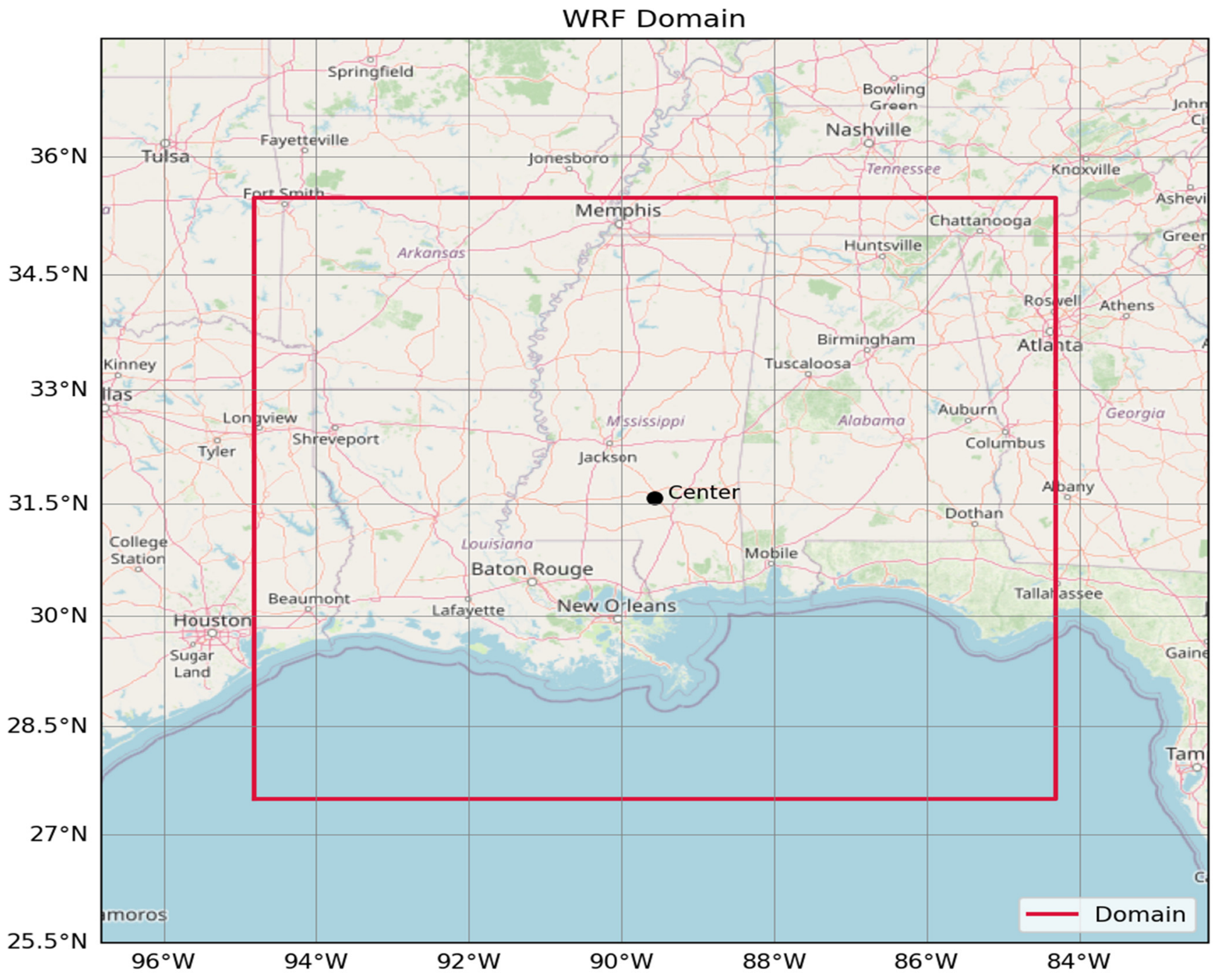
Table 1.
WRF physics configuration (fixed across all experiments).
Table 2.
WRF matrix configuration for all experiments.
The absence of a sub-kilometer nest, nevertheless, has consequences for interpreting the results. The effective resolution of WRF is approximately seven times the grid spacing [42], so at 4 km only features wider than about 28 km are well resolved. Individual convective updrafts, which are typically a few kilometers wide, are, therefore, under-resolved, and deep convection is not numerically converged at a kilometer-scale grid spacing, where simulated convective cells tend to be too large and too few [43]. Consequently, none of the configurations tested here can represent, cell by cell, the localized convective cores that produced the observed totals above 200 mm, and microscale processes, such as entrainment, cold-pool dynamics, and the fine structure of updraft microphysics, are captured only crudely. This is consistent with the results in Section 4.3, where the highest spatial skill emerges only at neighborhood scales of 20–40 km and no configuration reaches FSS ≥ 0.5 for the ≥200 mm threshold. A nested configuration with an inner domain of about 1 km or finer, run without deep-convection parameterization and conservatively upscaled to the Stage IV grid for verification, is a natural extension of this work (Section 5).
3.4. Physics Experiment Design
To assess the model’s sensitivity to physical parameterizations, an ensemble of 12 configurations was constructed by systematically combining two microphysics schemes with six cumulus parameterization schemes.
- Microphysics Schemes
- WDM6 (WRF Double-Moment 6-class)
This advanced double-moment scheme predicts both the mass mixing ratio and number concentration for different hydrometeor species. It incorporates aerosol–cloud interactions, thereby improving the representation of cloud droplet formation and precipitation development.
- Morrison Double-Moment Scheme
This widely used microphysics scheme predicts both mass and number concentrations for various hydrometeor categories. It provides improved treatment of mixed-phase processes and enhances the representation of stratiform precipitation, allowing for more accurate model predictions under different atmospheric conditions.
- Cumulus Parameterization Schemes
- Grell–Devenyi (GD):
An ensemble-based convective parameterization that employs multiple closure assumptions to address the inherent uncertainties associated with convective processes.
- Grell–Freitas (GF):
A scale-aware scheme that dynamically adapts convective tendencies to grid resolution, making it particularly well-suited for convection-permitting simulations and those within the transitional zone between large- and small-scale convection.
- Betts–Miller–Janjic (BMJ):
An adjustment-type scheme that stabilizes atmospheric profiles by nudging them toward reference thermodynamic states, proving especially effective in moist atmospheric contexts.
- Kain–Fritsch (KF):
A mass-flux parameterization that includes an intricate representation of entrainment and detrainment processes, coupled with a robust triggering mechanism that effectively initiates convection.
- KF-CuP (Kain–Fritsch with Convective Trigger Function):
An enhanced iteration of the Kain–Fritsch scheme that integrates an improved convective triggering function aimed at better depicting the timing of convective initiation.
- Tiedtke Scheme:
This mass-flux-based parameterization offers a comprehensive portrayal of shallow, mid-level, and deep convection, utilizing moisture convergence as a crucial component for model closure.
By varying these schemes, the study aims to discern their relative impacts on model performance, particularly in accurately capturing observed precipitation events.
Experiment Configuration Matrix
This study encompasses a detailed set of simulations organized into twelve distinct configurations designed to evaluate various model outputs across different parameters. The matrix configuration is detailed in Table 2.
Alongside the twelve primary configurations that were established for this study, we also executed two additional simulations where cumulus parameterization was intentionally disabled (indicated by setting cu_physics = 0). These simulations were designed to complement each of the microphysics schemes employed in our main configurations. The purpose of conducting these specific simulations was to serve as a bounding check, allowing us to assess the impact that cumulus parameterization has on the overall model results. Further details and insights regarding this analysis can be found in Section 4.6 of the research.
3.5. Data Processing and Regridding
To ensure a high degree of consistency between the outputs from the Weather Research and Forecasting (WRF) model and the actual observational data, a regridding process was applied to all WRF simulations. This process used the 4 km Stage IV grid to standardize the spatial resolution of the data. A conservative remapping technique was implemented using the xESMF (Extreme Scientific Computing Framework) library, chosen for its effectiveness in preserving the total volume of precipitation. This ensures that spatial comparisons between model outputs and observed datasets remain equitable and precise, thereby enhancing the validity of the simulation results.
3.6. Verification Framework
Model performance was assessed using a multi-metric verification framework that integrates traditional point-based statistics with spatial neighborhood verification and temporal diagnostics. All metrics were computed on the Stage IV HRAP 4 km grid after conservative regridding of WRF output via xESMF. Accumulation windows were aligned with the hourly availability of Stage IV data, and the FSS thresholds were set at Th ∈ {100 mm, 200 mm} with neighborhood scales at L ∈ {10, 20, 40} km.
- Accumulated Precipitation and Areal Exceedance
The domain-mean accumulated precipitation over the domain Ω for accumulation window T is represented as follows:
The fraction of grid cells meeting or exceeding a specified threshold, Th, is indicated by
where I [·] is the indicator function.
- Peak Intensity and Peak Error
Spatially, the maximum accumulated precipitation within Ω is calculated by
The signed difference between the modeled and observed peak values, where a positive result indicates overprediction, is given by
ΔPTmax = PT,WRFmax − PT,StageIVmax
- Grid-Point Error Statistics
All statistics calculated utilize F(i,j) and O(i,j) for the forecasted and observed accumulated precipitation (in mm) at grid cell (i,j), with N representing the number of grid cells in |Ω|:
The RMSE is designed to penalize larger errors more severely than the MAE; note that a bias of 0 does not necessarily reflect error-free forecasts due to potential cancellation effects. These metrics are sensitive to shifts in the spatial placement of precipitation features, which brings forth the double-penalty problem [36,37], thus setting the stage for the subsequent spatial verification metrics.
- Fractional Bias (FB)
The fractional bias serves as a balanced metric for evaluating the overall volumetric bias between the domain-mean forecast () and observed (Ō) precipitation, constrained to the valid Stage IV footprint:
where FB = 0 indicates perfect agreement between the forecast and observed totals. Positive FB values signify overestimation, while negative values indicate underestimation. The FB is constrained within [−2, +2], treating both over- and underforecasting symmetrically [40].
- Fractions Skill Score (FSS)
To compute the forecast and observed exceedance fraction fields within a square neighborhood N(i,j;L) centered at (i,j) and of scale L, the following formulation is employed:
The FSS ranges from 0 to 1. The useful-skill threshold is defined by an FSS > 0.5 + f_o/2. The minimum L at which the FSS(L) exceeds this threshold is termed the skillful scale [38].
- Spatial Pattern Correlation
The Pearson correlation between the forecasted and observed precipitation fields over Ω is given by
where and Ō are the respective domain means. A high correlation coefficient (r) indicates structural agreement but is less sensitive to magnitude bias; thus, it should be interpreted alongside the FSS and FB to provide a comprehensive evaluation.
4. Results and Discussion
This section presents a detailed assessment of twelve configurations of the Weather Research and Forecasting (WRF) model, each using two double-moment microphysics (MP) schemes: WDM6 and Morrison (MORR). Each MP scheme was paired with one of six cumulus parameterization (CP) schemes: Kain–Fritsch (KF), KF with Cumulus Potential (KF-CuP), Betts–Miller–Janjic (BMJ), Tiedtke, Grell–Freitas, and Grell–Devenyi.
The evaluation was comprehensive, employing both traditional point-based error statistics and neighborhood-based spatial verification methods, particularly the Fractions Skill Score (FSS). An analysis of the spatial pattern correlation and temporal precipitation accumulation was also conducted. All model outputs were validated against Stage IV radar-gauge composite observations, focusing on a notable extreme precipitation event from 27 April to 3 May 2014, spanning the Alabama–Mississippi region.
4.1. Total Domain-Averaged Precipitation
In the context of the specified meteorological event, the total domain-mean precipitation recorded from Stage IV observations amounted to 42.48 mm. This measurement was derived from a specific subset of the WRF model domain that had valid Stage IV coverage. It is important to note that the complete model domain encompasses areas that extend beyond the coverage of the radar-gauge network, notably including regions over the Gulf of Mexico. Therefore, the domain-mean statistics that have been reported apply solely to those grid cells that possess valid Stage IV observations.
Within this framework, the twelve primary configurations of the model were assessed alongside two control runs that did not incorporate cumulus parameterization (as described in Section 4.6). The analysis revealed a considerable range of variability in the predicted precipitation totals across these configurations. The lowest total recorded was 18.61 mm for the WDM6_BMJ configuration, which represented a significant negative deviation of −56.2% when compared with the observed precipitation. Conversely, the highest predicted total was 47.64 mm for the MORR_KF configuration, which resulted in a positive deviation of +12.1%.
One configuration of particular interest was the WDM6_KF-CuP, which exhibited the closest alignment to the observed data, producing a total of 41.95 mm and a minimal deviation of just −1.2%. This marked performance underscores the sensitivity of accumulated precipitation estimates to the selection of the cumulus parameterization scheme utilized within the model framework. For a more comprehensive overview of the domain-mean precipitation totals for all evaluated configurations, including detailed performance metrics, readers are referred to Table 3 and Figure 2.
Table 3.
The domain-mean event-total precipitation (mm) for the twelve primary WRF configurations plus the two no-cumulus control simulations (Section 4.6) compared with the Stage IV observations (42.48 mm), computed over the common valid coverage footprint (see Section 3.6). Bias and percentage difference are calculated as model output minus observed values. The observed benchmark is at the top, with the highest-ranked configuration (WDM6_KF-CuP) highlighted in bold. The two no-cumulus runs are labeled accordingly in the “Notes” column; they were not part of the original twelve-member physics matrix and are included here for direct comparison, consistent with Section 4.6. A dash (—) indicates not applicable.
Figure 2.
Comparison of WRF storm-total domain-mean precipitation estimates (mm) across the twelve primary physics configurations plus the two no-cumulus control simulations (Section 4.6) against the Stage IV observed mean (42.48 mm, red dashed line), computed over the valid Stage IV coverage footprint.
- Sensitivity to Cumulus Parameterization
The precipitation variability driven by CP, as documented in Table 3, underscores fundamentally different triggering and closure characteristics across CP scheme families. The MORR_KF configuration yielded the highest total rainfall, recording 47.64 mm over the common verification footprint, corresponding to an overestimation of 12.1% relative to the observed data. In contrast, the WDM6_KF-CuP configuration provided a more accurate domain-mean precipitation of 41.95 mm, reflecting a slight deviation of just 1.2%.
Other CP configurations, such as the Grell–Freitas and Tiedtke schemes, exhibited significant underestimation of total precipitation, with domain means ranging from 29.35 to 30.53 mm (Grell–Freitas) and 29.01 to 29.84 mm (Tiedtke), resulting in biases of around −28% to −32%. This performance tier aligns more closely with BMJ than with the upper echelon of the KF-family and Grell–Devenyi configurations. The BMJ schemes consistently underperformed, with WDM6_BMJ recording only 18.61 mm (a deficit of 56.2%) and MORR_BMJ achieving 20.02 mm (a deficit of 52.9%). The limitations of the BMJ scheme can be traced to its structural characteristics as a relaxation-type scheme; lacking explicit updraft and downdraft dynamics, it fails to sustain the convective intensity typical of training MCS episodes, regardless of the surrounding moisture environment.
- Sensitivity to Microphysics Scheme
Compared with the WDM6 configurations, the MORR configuration consistently yielded marginally higher precipitation totals. This can be attributed to the Morrison scheme’s five-species number-concentration prognostic, which enhances the efficiency of vapor-to-precipitation conversion during deep convective processes. As a result, higher precipitation totals are systematically observed across all CP pairings, particularly pronounced in instances of aggressive convective triggering, aligning with the CP sensitivity discussed in Section 4.1.
Conversely, the WDM6 scheme, which incorporates explicit predictions for cloud condensation nuclei (CCN), tends to dampen raindrop growth rates. The autoconversion suppression linked to CCN dynamics in WDM6 serves as a physical moderator against the overestimation of precipitation anticipated from CP processes, as outlined in Section 4.1. This interaction is further explored in the ensuing spatial verification results.
4.2. Traditional Verification Metrics
Table 4 presents the point-to-point verification statistics, detailing critical performance metrics, such as mean bias, root mean square error (RMSE), mean absolute error (MAE), and fractional bias (FB) for the twelve evaluated model configurations. The arrows next to the MORR values indicate performance changes relative to the WDM6 baseline, showing improvements (↑), degradations (↓), or parity (→) for the corresponding cumulus parameterization (CP) schemes.
Table 4.
Verification metrics for the twelve primary WRF configurations plus the two no-cumulus control runs (Section 4.6): mean bias (mm), RMSE (mm), MAE (mm), and FB. Bolded values highlight the two top-performing configurations for each metric across the columns; arrows indicate whether MORR improved (↑) or degraded (↓) relative to WDM6 for each pairing.
4.2.1. Bias and Fractional Bias
Among the configurations analyzed for bias, WDM6_KF-CuP and WDM6_Kain–Fritsch stood out for their minimal bias. Specifically, WDM6_KF-CuP registered a negative bias of −0.53 mm and an FB of −0.013, while WDM6_Kain–Fritsch showed a slight positive bias of +1.73 mm with an FB of +0.040. These results underscore their status as among the most volumetrically accurate configurations, as reflected in Table 4.
In contrast, the BMJ configurations showed significant negative biases, with WDM6_BMJ at −23.87 mm with an FB of −0.782 and MORR_BMJ at −22.46 mm with an FB of −0.719. The moderate systematic underestimation indicated by the FB values for the Tiedtke scheme (approximately −0.35 to −0.38) and the Grell–Freitas scheme (around −0.33 to −0.37) points to the need for accuracy enhancements. Additionally, configurations using the Kain–Fritsch and KF-CuP methods generally reported positive FB values (WDM6_KF-CuP, at −0.013, is the exception), aligning with the volume overestimation noted in Section 4.1.
4.2.2. Error Magnitude
The MORR_BMJ configuration achieved the lowest RMSE of 55.85 mm and MAE of 32.42 mm across all twelve configurations analyzed. However, these figures warrant cautious interpretation. The BMJ scheme’s low error metrics stem not from accurately capturing high-intensity rainfall events but from consistently underforecasting them, thereby avoiding the serious displacement penalties commonly associated with high-resolution convective forecasts. This observation is reinforced by the near-zero FSS values noted in Section 4.3. Conversely, the MORR_Kain–Fritsch configuration exhibited the highest RMSE at 70.86 mm and MAE at 41.42 mm, highlighting the drawbacks of aggressive overestimation.
In configurations that effectively capture convective structures, especially those within the KF and GF families, the differences in RMSE and MAE between the WDM6 and MORR schemes were minimal (≤2 mm), indicating comparable accuracy when paired with an appropriately triggering convective parameterization scheme.
4.3. Spatial Verification: Fractions Skill Score
To address the well-known double-penalty issue in high-resolution convective verification, the Fractions Skill Score (FSS) was computed at two intensity thresholds (≥100 mm and ≥200 mm) across three neighborhood scales (10 km, 20 km, and 40 km). The results are presented in Table 5 and shown in the heatmap in Figure 3. This comprehensive evaluation aims to improve the understanding of the spatial performance of various configurations in predicting precipitation events.
Table 5.
Details of the FSS outcomes for the twelve primary WRF configurations plus the two no-cumulus control runs (Section 4.6) at the specified thresholds and neighborhood scales, with arrows indicating changes relative to the WDM6 baseline for each pairing (↑, improvement; ↓, degradation; →, no change). Bold values signify the two highest-scoring entries in each column across all configurations.
Figure 3.
Heatmap of the normalized Fractions Skill Score (FSS) values across multiple precipitation thresholds (≥100 mm and ≥200 mm) and neighborhood scales (10 km, 20 km, and 40 km).
Scale Dependence
The Fractions Skill Score (FSS) analysis reaffirmed the configuration hierarchy outlined in Section 4.1, with the KF-family configurations consistently outperforming and the BMJ configurations registering nearly zero scores across all thresholds and scales (see Table 5). A significant finding from the spatial verification phase was that no configuration achieved the useful-skill threshold (FSS ≥ 0.5) at the ≥200 mm precipitation intensity level across any evaluated scale. The highest FSS observed was 0.349 (WDM6–KF-CuP at the 40 km scale), as shown in Figure 3.
Threshold Performance
At the ≥100 mm precipitation threshold, the WDM6_Kain–Fritsch configuration achieved the highest FSS of 0.486 at the 40 km scale, closely followed by WDM6_KF-CuP with an FSS of 0.480. Among the Grell–Devenyi schemes, the MORR_Grell–Devenyi configuration achieved an FSS of 0.447 at the same scale, making it the top Grell–Devenyi option. The MORR configuration consistently outperformed WDM6 across all tested scales and thresholds for both the Grell–Devenyi and Tiedtke families of schemes. In contrast, at the more challenging ≥200 mm threshold, WDM6_KF-CuP led with an FSS of 0.349, followed by WDM6_Kain–Fritsch at 0.322. This skill differential between the KF family and BMJ at various spatial scales parallels the volumetric discrepancies identified in Section 4.1; configurations that struggle to sustain convective intensity similarly fail to generate spatially coherent precipitation cores (as shown in Table 5).
Microphysics Influence on FSS
The interplay between microphysics and convective parameterization (CP) highlighted in Section 4.2 is particularly evident in the FSS outcomes, where the advantage of WDM6 over Morrison reverses across different cumulus pairings. The MORR scheme consistently outperformed WDM6 within the Grell–Devenyi context, demonstrating an improvement of +0.083 at the ≥200 mm threshold at the 40 km scale. Similar gains were noted for the Tiedtke pairing, which saw an enhancement of +0.057 at the same threshold and scale. Conversely, the WDM6 configuration outperformed MORR within the Kain–Fritsch pairing (showing a +0.021 improvement) and the KF-CuP pairing (+0.045), as well as the Grell–Freitas scheme, which noted a +0.072 increase at the extreme ≥200 mm threshold. This indicates that the cloud condensation nuclei (CCN)-aware double-moment rainfall physics inherent in WDM6 effectively concentrates extreme rainfall into more localized and well-defined spatial cores when paired with highly convective CP schemes.
4.4. Composite Ranking
To effectively distinguish among various configurations that might be indistinguishable based on single metrics alone, a robust composite scoring system has been developed. This system places particular emphasis on the Fractions Skill Score (FSS) at the ≥200 mm rainfall threshold, using a weighted approach: 0.40 for the 40 km scale, 0.20 for the 20 km scale, and 0.10 for the 10 km scale. Additionally, the FSS at the ≥100 mm threshold is weighted at 0.20 specifically for the 40 km scale.
In enhancing the scoring system’s accuracy, minor penalties have been incorporated for several metrics that could potentially skew the results. These include frequency bias (FB), which carries a penalty weight of 0.05, and various error metrics such as bias, root mean square error (RMSE), and mean absolute error (MAE), which are assigned lighter penalties of 0.025, 0.0125, and 0.0125, respectively. All components of the scoring system undergo min–max normalization to a [0, 1] range to ensure comparability.
The rationale behind prioritizing the most extreme rainfall threshold in this composite scoring scheme is to address a known issue in traditional point-to-point metrics, specifically the double-penalty phenomenon associated with metrics like bias and RMSE. Such metrics can inadvertently encourage forecasts that downplay extreme rainfall amounts rather than represent them accurately. By assigning a higher weight to the FSS at the threshold that reflects severe precipitation events, this composite ranking system seeks to favor configurations that successfully capture organized structures of extreme precipitation, which is vital for hazard assessment and risk management in meteorological contexts.
The summarized results of this composite evaluation are documented in Table 6, which lists the ten Weather Research and Forecasting (WRF) configurations that received a finite score according to this comprehensive weighting scheme. These configurations are arranged in descending order from the highest-ranked (best-performing) to the lowest. Noteworthy among the results is that the configuration labeled WDM6_KF-CuP ranks at the top, followed closely by WDM6_Kain–Fritsch. It is important to highlight that the performance metrics for the KF-CuP variant also include data from the complete 12-configuration dataset as part of the full metrics evaluation, which encompasses the MORR_KF-CuP setup.
Table 6.
Composite ranking of the ten WRF configurations for which a finite composite score could be computed under this weighting scheme. The two BMJ configurations (WDM6_BMJ and MORR_BMJ) are excluded from this ranking due to their FSS values being at or near zero across all thresholds and scales evaluated (refer to Table 5), which would position them at the lowest tier of every FSS-weighted component. The two no-cumulus control runs (Section 4.6) are also excluded, since they represent the absence of a cumulus scheme rather than a rival scheme choice within this CP-scheme comparison; their full metrics are reported in Table 3, Table 4 and Table 5 and Section 4.6.
Conversely, the two configurations utilizing the Betts–Miller–Janjic (BMJ) scheme (namely, WDM6_BMJ and MORR_BMJ) have been excluded from this ranking. Their FSS values were either at or near zero across all evaluated thresholds and scales (as detailed in Table 5), meaning they would rank at the lowest level for every FSS-weighted component, thus offering no further distinguishing insights beyond those reflected in Table 3, Table 4 and Table 5.
Additionally, the two control runs that omit the cumulus parameterization (introduced in Section 4.6) are also excluded from this ranking. This exclusion is due to their nature; since they do not employ a cumulus scheme, they cannot be considered a valid competing option within this comparative analysis of cumulus parameterization schemes. Including these control runs would conflate two separate analytical questions. The detailed metrics for these no-cumulus runs—including bias, RMSE, MAE, FB, FSS, and convective timing—are comprehensively reported in Table 3, Table 4 and Table 5 and Section 4.6.
In conclusion, Table 6 offers a clear composite ranking of the applicable ten WRF configurations, highlighting their distinct performances under the defined scoring criteria while providing clarity on the exclusions made for configurations that do not meet the necessary thresholds for meaningful comparison.
The comprehensive composite analysis confirmed the predicted hierarchy at the top of the performance rankings, with the WDM6–KF-CuP configuration taking the lead, followed closely by the WDM6–Kain–Fritsch model. This ordering aligns with the convective parameterization (CP) hierarchy previously outlined in Section 4.1, Section 4.2 and Section 4.3 of the study. It is worth noting that the two configurations utilizing the BMJ model were intentionally omitted from Table 6, as explained in the table’s caption. Despite their absence from the composite ranking, both BMJ configurations consistently demonstrated inferior performance across all metrics, as detailed in Table 3, Table 4 and Table 5.
The primary significance of the composite ranking lies in its ability to clarify the mid-tier ordering among various configurations, an aspect that specific individual metrics failed to highlight. Among the mid-tier options, the WDM6–GF, MORR–GD, and MORR–GF models exhibited similar domain-mean values and displayed overlapping FSS curves. Nevertheless, their respective composite scores, which are 0.713 for WDM6–GF, 0.639 for MORR–GD, and 0.538 for MORR–GF, reveal substantial differences in the delicate balance between spatial skill and volumetric accuracy.
In particular, the WDM6–GF model’s superior FSS for precipitation levels exceeding 200 mm effectively compensates for its greater volumetric bias when compared with MORR–GD. This nuanced relationship is a critical insight that is only brought to light by the weighted composite analysis, underscoring the importance of this ranking method in understanding the performance of these configurations. For further visualization and detailed comparisons, please refer to Table 6 and Figure 4, which illustrate these findings in greater depth.
Figure 4.
Bar chart of FSS ≥ 200 mm at 40 km for all configurations.
Spatial Pattern Correlation
To evaluate the structural fidelity of the precipitation fields without intensity bias, Pearson correlation coefficients (r) were computed for each model configuration against the Stage IV observational data at thresholds of ≥100 mm and ≥200 mm. The analysis spanned spatial scales of 10 km, 20 km, and 40 km, and the results are summarized in Table 7.
Table 7.
Spatial Pearson pattern correlation coefficients (r) between each WRF configuration and Stage IV observations at ≥100 mm and ≥200 mm thresholds across 10, 20, and 40 km neighborhood scales. Bold values denote consistently top-performing configurations. Values at 30 km are omitted for brevity; 40 km values are shown for the ≥200 mm threshold only.
- Performance at the ≥100 mm Threshold
At the ≥100 mm precipitation threshold, a distinct hierarchy among the CP schemes emerged. Both the Grell–Devenyi and KF-family configurations exhibited enhanced performance, accurately representing the broad precipitation distribution typical of significant rainfall events. Notably, the MORR_Grell–Devenyi configuration achieved the highest correlation at the 40 km scale, with a correlation coefficient of approximately 0.52, as detailed in Table 7 and illustrated in Figure 5. Generally, configurations utilizing MORR demonstrated slightly higher correlation values than their WDM6 counterparts, averaging an improvement of about 0.05 in the correlation coefficient (r). This finding suggests that the MORR approach to hydrometeor growth simulation yields a more coherent depiction of moderate-intensity rainfall across spatial domains. However, the WDM6_Tiedtke scheme emerged as a notable outlier, presenting negative correlations (r ≈ −0.07 at 10 km), indicative of a systematic phase error in which the model mislocalized heavy rainfall, predicting it in regions of minimal precipitation accumulation according to Stage IV data, as shown in Figure 5.
Figure 5.
Pattern correlation vs. spatial scale (obs mask; box mean smoothing): (top) ≥100 mm and (bottom) ≥200 mm, with both having one line per configuration (12 total). Correlation increases with neighborhood size (10 → 40 km), diagnosing predominantly positional error.
- Performance at the ≥200 mm Threshold
When analyzing the ≥200 mm extreme precipitation threshold, a clear trend emerged: all model configurations exhibited higher correlation values with increasing spatial scale. This supports the notion that maintaining structural integrity at the meso-β scale is more effective than concentrating on precipitation placement at the cell scale. Specifically, the MORR_Grell–Devenyi scheme attained the highest correlation at the 40 km scale (r ≈ 0.63). In contrast, the WDM6_KF-CuP configuration demonstrated stable, high skill across various spatial scales, achieving a correlation of approximately 0.50 at 40 km (as shown in Table 7). Conversely, the BMJ and Grell–Freitas schemes displayed inadequate structural fidelity at this extreme threshold, with correlation coefficients falling below 0.25, highlighting their difficulties in generating organized convective cores crucial for accurate precipitation forecasting. While the WDM6_Tiedtke scheme exhibited a modest recovery at the ≥200 mm threshold (r ≈ 0.07 at 40 km), this suggests that when it does forecast extreme precipitation events, the placement of those predictions aligns more accurately with observed heavy precipitation cores compared with its performance for moderate rainfall events, as depicted in Table 7 and Figure 5.
4.5. Temporal Precipitation Analysis
To contextualize and deepen the understanding of the bulk spatial verification metrics, a domain-averaged time-series analysis was conducted. This analysis juxtaposed Stage IV precipitation observations against three representative configurations: WDM6_KF-CuP (first in performance ranking), WDM6_Kain–Fritsch (second), and WDM6_BMJ (lowest-performing; excluded from the composite ranking), as illustrated in Figure 6a–c.
Figure 6.
(a) Domain-averaged time-series analysis comparing hourly precipitation intensity (mm h−1) for the selected runs; (b) domain-averaged time-series analysis comparing hourly precipitation intensity (mm h−1) and cumulative accumulation (mm) for the selected runs; (c) normalized temporal peak alignment analysis.
4.5.1. Temporal Evolution of Precipitation Intensity
The Stage IV observational data captured a distinctive meteorological event marked by a primary high-intensity precipitation peak, registering approximately 1.5 to 2.0 mm h−1 between 29 and 30 April. Following this, a smaller secondary pulse of rain was noted (Figure 6a). The WDM6_BMJ configuration demonstrated conservative performance, rarely exceeding 0.5 mm h−1, which contributed to its favorable low root mean square error (RMSE) and mean absolute error (MAE). However, this also resulted in a nearly negligible Fractions Skill Score (FSS), as the model consistently refrained from predicting significant rainfall amounts. On the opposite end, the WDM6_Kain–Fritsch configuration exhibited aggressive convective triggering, producing sharp peaks that surpassed 3.0 mm h−1, indicating a notable overestimation of peak intensity. In contrast, the WDM6_KF-CuP scheme displayed a more moderate response, achieving a peak intensity around 2.5 mm h−1. This configuration effectively limited explosive updrafts relative to the standard Kain–Fritsch scheme while still capturing the severity of the observed precipitation event.
4.5.2. Cumulative Precipitation Accumulation
The cumulative domain-averaged rainfall plot shows the integral of intensity biases accumulated over the entire simulation period (Figure 6b), computed over the same valid Stage IV observation footprint used for Table 3 (Section 3.6). Stage IV data indicate a total accumulation of 43.71 mm. The WDM6_BMJ scheme consistently generated precipitation totals well below the observed rate, culminating at 19.21 mm (−56.1%), consistent with its behavior in Table 3. The WDM6_Kain–Fritsch simulation overestimated the total accumulation, reaching 45.65 mm (+4.4%), while the WDM6_KF-CuP simulation ended just below the observed total, at 43.30 mm (−0.9%), closely tracking the near-zero domain-mean bias already reported in Table 3 and Table 4. Even so, the temporal analysis shows that this near-zero net bias for WDM6_KF-CuP conceals real within-event variability: as detailed above, it visibly overestimates intensity during the second (30 April) precipitation peak while more closely matching the first (29 April) peak. The near-zero cumulative total, therefore, reflects partially offsetting errors across the two peaks of the event rather than uniformly accurate performance throughout.
Convective Timing and Phase Alignment
A detailed examination of the normalized peak timing for precipitation events revealed noteworthy findings regarding the performance of both the KF (Kain–Fritsch) and KF-CuP (Kain–Fritsch with CuP parameterization) schemes. Both schemes demonstrated a collective tendency to initiate convective activity prematurely when compared with Stage IV observations, with a substantial aggregate lead of approximately 2 h identified through cross-correlation analysis. This early onset of convection suggests a potential systematic bias in the modeling approaches used.
The precipitation event under consideration was characterized by a broad and sustained peak that persisted well into April 30, highlighting the complexity and duration of the rainfall. When comparing the two schemes, the standard KF scheme exhibited a distinct and sharp early peak in precipitation followed by a rapid decline in rainfall intensity. This pattern indicates a tendency for the KF scheme to overestimate early convective development without adequately capturing the subsequent rainfall dynamics.
In contrast, the KF-CuP scheme displayed a more nuanced behavior, managing to broaden the simulated precipitation peak while also extending the overall duration of rainfall compared with the KF scheme. However, it is important to note that despite these improvements, the KF-CuP scheme did not completely mitigate the overarching early bias associated with both modeling approaches when compared with the observed Stage IV data.
Looking ahead, there is significant potential for future iterations of the WRF (Weather Research and Forecasting) framework that implements the KF-CuP parameterization to achieve better accuracy. By making tailored adjustments to the convective trigger functions, it may be possible to delay the onset of convection effectively. Such modifications could help align the modeling outputs more closely with the observed diurnal characteristics of precipitation events, ultimately improving the fidelity of precipitation forecasts.
Double-Moment Microphysics Inter-Comparison: MORR vs. WDM6
This comprehensive analysis evaluates the performance metrics of six cumulus parameterization (CP) schemes, focusing on the two double-moment microphysics implementations: Morrison (MORR) and WDM6. The results from these schemes have been aggregated across all six cumulus schemes, including the KF-CuP scheme, now that its verification statistics have been finalized. The findings indicate that while both MORR and WDM6 possess unique strengths, they also exhibit complementary attributes that highlight their respective advantages across different environmental scenarios (Table 8).
Table 8.
Aggregated verification metrics mean values for WDM6 and Morrison (MORR) double-moment microphysics schemes, averaged across all six cumulus schemes (Grell–Devenyi, Tiedtke, BMJ, Grell–Freitas, Kain–Fritsch, and KF-CuP). The “Winner” column identifies the scheme excelling in each metric, with bold values indicating the winning scheme’s score. FB: fractional bias (0 = ideal). FSS pertains to data from the complete metrics run for ≥300 mm. * The Composite Score is averaged across five schemes only (it excludes BMJ), since Table 6 does not report a composite score for the BMJ configurations (see Table 6 caption). A dash (—) indicates not applicable.
Bulk Error Statistics and Volume Fidelity
When traditional error metrics are assessed, Morrison’s methodology shows a notable advantage over the WDM6 model, as shown in Table 8. A deeper analysis reveals that the mean bias (MB) for MORR was −6.80 mm, indicating a smaller deviation from observed values than WDM6’s −8.44 mm. This reduction in mean bias suggests that MORR may offer more accurate predictions relative to the actual measurements.
Additionally, the root mean square error (RMSE), which reflects the model’s variance and predictive accuracy, was 64.93 mm for MORR. This value is marginally better than WDM6’s 65.02 mm. The negligible difference in RMSE highlights MORR’s proficiency in closely aligning its predictions with observed data while maintaining a lower error margin.
The mean absolute error (MAE) provides further corroboration of these findings, with MORR reporting 37.98 mm compared with WDM6’s 38.26 mm. The MAE’s role in quantifying the average magnitude of errors in predictions also emphasizes that MORR’s performance slightly edges out WDM6’s in terms of absolute accuracy.
Moreover, the fractional bias (FB), which assesses bias relative to the size of the mean observation, was −0.210 for MORR, indicating it is closer to neutral than WDM6’s −0.255. This information suggests that MORR has a more balanced tendency regarding over- and underpredictions. However, it is critical to note that while these metrics indicate a consistent directional superiority for MORR, the differences observed did not achieve statistical significance at the α = 0.05 level. This conclusion stems from the Wilcoxon signed-rank tests detailed in Section 4.5.3 across six paired cumulus configurations, a sample too small to establish either a difference or equivalence.
Thus, while these results hint at a potential advantage for MORR, they must be interpreted cautiously as suggestive rather than definitive evidence of its superiority over WDM6. This observation aligns with the strengths of MORR, which incorporates a well-rounded approach to predicting five distinct species of number concentration. This comprehensive modeling choice enhances the simulation of hydrometeor growth and sedimentation processes, particularly in environments characterized by deep convective activity. Overall, these insights highlight the implications of model selection in improving accuracy in meteorological predictions.
Spatial Skill and Extreme-Threshold Performance
When evaluating spatial skill at moderate precipitation thresholds, the MORR model demonstrated a significant advantage, achieving a Fractions Skill Score (FSS) of 0.341 for precipitation thresholds of 100 mm or more when assessed at a spatial resolution of 40 km. This performance not only surpassed WDM6, which recorded an FSS of 0.330, but also indicated MORR’s superior capability in capturing the spatial distribution of rainfall in this range. Moving to the higher threshold of 200 mm, both models displayed a remarkable alignment in skill level, with both MORR and WDM6 reporting an identical FSS of 0.174 when rounded to three decimal places, as detailed in Table 8.
However, an interesting shift in performance was observed at the extreme precipitation threshold of 300 mm and above. In this instance, WDM6 outperformed MORR, achieving an average FSS of 0.108 compared with MORR’s 0.078. This finding implies that WDM6’s cloud condensation nuclei (CCN)-aware, double-moment rain parameterization is particularly effective at localizing convective responses, allowing it to concentrate precipitation in distinct core areas. This characteristic likely enhances WDM6’s alignment with Stage IV observations that capture the most intense rainfall events. Such a capability can be particularly valuable for applications focused on forecasting extreme weather, even though WDM6 tends to underestimate total precipitation amounts over larger areas.
Additionally, when calculating the composite score across the five non-BMJ schemes for which data are presented in Table 6, WDM6 narrowly edged out MORR with a score of 0.654 compared with 0.652. This reflects the considerable influence of the KF-CuP scheme on WDM6’s average score, highlighting its disproportionate contribution compared with the other four models included in the evaluation.
4.5.3. CP-Dependent Microphysical Sensitivity
The differential performance of MORR and WDM6 was significantly affected by the convective parameterization (CP) schemes used. MORR showed the greatest improvements when paired with the Grell–Devenyi and Tiedtke schemes, suggesting that these configurations provide an optimal environment for MORR’s enhanced representation of the hydrometeor spectrum.
Conversely, WDM6 performed better with the Kain–Fritsch, KF-CuP, and Grell–Freitas schemes, which are typically associated with more vigorous convective activity.
This implies that in environments characterized by intense convection, WDM6’s CCN feedback and refined double-moment representation of rainfall more effectively capture microphysical processes, producing well-defined, localized precipitation cores. This interaction between microphysics and cloud physics is a crucial finding that could inform future physics suite selections for high-impact weather prediction, particularly in the southeastern United States.
Synthesis: Best-Performing Configuration in This Case Study
An extensive evaluation employing five distinct verification methodologies indicates that the WDM6_KF-CuP configuration demonstrated superior performance in simulating the April–May 2014 extreme precipitation event in Alabama. This assessment utilized domain-mean precipitation (Table 3 and Figure 2), standard error statistics (Table 4), FSS spatial verification techniques (Table 5 and Figure 3), composite scoring (Table 6 and Figure 4), spatial pattern correlation (Table 7 and Figure 5), and temporal analysis (Figure 6). However, it is important to note that these findings are specific to this singular event and should not be generalized across the broader region.
The key findings supporting the WDM6_KF-CuP’s performance include the following:
- It exhibited the lowest domain-mean bias at −0.53 mm, alongside a fractional bias (FB) of nearly zero at −0.013;
- The configuration achieved the highest composite score of 0.980, primarily resulting from its strong FSS at the ≥200 mm extreme threshold (FSS@40 km = 0.349);
- Stable spatial pattern correlations were maintained across scales, with r ≈ 0.49 at 40 km for the ≥200 mm threshold;
- WDM6_KF-CuP also demonstrated improved temporal modulation of convective intensity compared with the standard Kain–Fritsch scheme.
The composite score of 0.980 reflects the specific weighting scheme described in Section 4.4, showcasing a strong relative performance rather than absolute forecast skill. This is further highlighted by the FSS value of 0.349 at the ≥200 mm/40 km threshold, which does not meet the conventional 0.5 useful-skill benchmark. Thus, while WDM6_KF-CuP is justifiably termed the best-performing configuration among those tested, it should not be described as “skillful” or “effective” in an absolute sense.
The WDM6_Kain–Fritsch combination closely followed with a composite score of 0.927, showing a solid performance across the evaluation criteria. It recorded the highest FSS at the ≥100 mm threshold (FSS@40 km = 0.486) and superior spatial pattern correlation among single-scheme configurations, albeit accompanied by a noticeable positive domain bias. For assessments focusing on total precipitation volume, both the WDM6_Grell–Devenyi and MORR_Grell–Devenyi configurations provided accurate estimates (41.14 mm and 40.84 mm, respectively, with biases of −3.2% and −3.9%). Conversely, WDM6_Grell–Freitas significantly underestimated precipitation (29.35 mm; −30.9%), while MORR_Grell–Freitas and MORR_Tiedtke also displayed considerable underestimations (30.53 mm and 29.84 mm; −28.1% and −29.8%).
The BMJ scheme consistently underperformed across all microphysics configurations, primarily due to its convective-adjustment methodology, which inhibited the development of organized convective cores. This led to negligible FSS values at both the ≥100 mm and ≥200 mm thresholds, along with significant volumetric deficits—aligning with established limitations of the BMJ scheme in environments with organized deep convection.
Future research should focus on identifying skillful-scale thresholds beyond the current 40 km resolution limit and exploring adjustments to convective triggers in KF-CuP to mitigate the documented phase bias observed in previous temporal analyses.
Spatial Evaluation of Convective Core Placement
For spatial evaluation of convective core placement, a qualitative review of storm-total precipitation fields (see Figure 7) enhances our understanding of statistical metrics. Specifically, the Tiedtke configurations demonstrate a strong ability to capture the mesoscale convective system’s spatial orientation. However, a notable issue arises from point-to-point misalignment of intensity maxima, leading to the “double-penalty” error traditionally found in evaluation metrics. Despite this displacement, the model maintains a commendable level of volumetric accuracy, which is vital for assessing overall precipitation effectiveness.
Figure 7.
Spatial distribution of total precipitation (mm) for Stage IV observations versus WRF simulations. Note the NW–SE rain band alignment.
Aggregate Comparison of Double-Moment Microphysics: Morrison vs. WDM6
To assess the effect of microphysical parameterization on simulation outcomes for the intense precipitation event of April–May 2014, we combined results from six cumulus configurations across both microphysics schemes. This aggregation strengthens comparisons between the Morrison (MORR) and WDM6 double-moment schemes, thereby reducing the variability associated with individual cumulus parameterizations.
Although both schemes employ double-moment formulations, they differ considerably in their treatment of hydrometeor size distributions, aerosol interactions, and phase processes. These methodological variations significantly influence precipitation intensity and spatial organization, which are critical aspects of meteorological modeling.
Impact on Rainfall Intensity and Bulk Error Characteristics
The aggregated statistical results shown in Table 9 indicate a persistent dry bias for both microphysics schemes when compared with Stage IV observational data. However, significant discrepancies arise in their ability to accurately replicate storm-total precipitation.
Table 9.
Aggregate performance of double-moment microphysics schemes (Morrison and WDM6) averaged across all six cumulus parameterizations for the April–May 2014 extreme precipitation event. Metrics include mean absolute error (MAE), root mean square error (RMSE), bias, and fractional bias (FB), evaluated against Stage IV observations. Negative bias values indicate systematic underestimation of precipitation totals.
The MORR scheme exhibits superior volumetric performance, with a mean bias of −6.80 mm, compared with WDM6’s −8.44 mm. This difference is substantiated by the fractional bias (FB) metrics, where MORR achieves an FB of −0.210, indicating less underestimation than WDM6’s FB of −0.255. The reduced bias of the MORR scheme implies a more effective representation of precipitation processes during the peak convective phases, likely driven by its intricate modeling of mixed-phase microphysical processes critical to such intense events.
While the differences in the overall error magnitudes between the two schemes are not dramatic, they remain consistently observable across various metrics. For example, MORR reports a mean absolute error (MAE) of 37.98 mm compared with WDM6’s 38.26 mm, along with a root mean square error (RMSE) of 64.93 mm versus 65.02 mm for WDM6. Although these variations are modest, their consistency across all bulk metrics reinforces the reliability of the MORR scheme for estimating total precipitation accumulation during this event.
Impact on Spatial Structure and Scale-Dependent Skill
Spatial verification employing the Fractions Skill Score (FSS), as detailed in Table 5 and illustrated in Figure 3, allows for a detailed comparison of the two microphysics schemes, highlighting the trade-off between the representation of large-scale precipitation and localized extreme intensity features.
At the moderate precipitation threshold of ≥100 mm, the MORR scheme consistently outperforms WDM6 across multiple neighborhood scales, achieving an FSS of 0.341 at the 40 km scale compared with WDM6’s 0.330. This enhancement underscores MORR’s superior capability in accurately capturing both the spatial extent and continuity of rainfall fields.
In contrast, at the extreme precipitation threshold of ≥200 mm, a scale-dependent disparity in performance emerges. At coarser scales (40 km), both schemes yield nearly equivalent FSS values (around 0.174). However, at finer scales (20 km and 10 km), WDM6 exhibits a slight edge, with FSS values of 0.156 and 0.141, respectively, compared with MORR’s 0.154 and 0.137. Although these differences are minor, their consistent occurrence indicates that WDM6 is better suited for resolving high-intensity localized precipitation cores.
These insights, as shown in Figure 8, illustrate that while the MORR scheme excels in representing broader precipitation structures, the WDM6 scheme provides improved accuracy in capturing concentrated extreme rainfall features. This complexity highlights the inherent challenges in accurately simulating convective precipitation processes.
Figure 8.
Comparison of the Fractions Skill Score (FSS) between the Morrison and WDM6 microphysics schemes at the ≥200 mm precipitation threshold across multiple spatial neighborhood scales (10–40 km). Higher FSS values indicate improved spatial agreement with the Stage IV observations. The figure highlights scale-dependent differences in the ability of each scheme to resolve extreme precipitation structures.
Interpretation of Microphysical Sensitivities
The disparities observed between the Morrison (MORR) and WDM6 microphysical schemes arise from their fundamentally distinct formulations and the way they represent physical processes. MORR exhibits enhanced volumetric performance, largely due to its comprehensive approach of incorporating multiple hydrometeor species. This includes the implementation of prognostic number concentrations for various precipitation types, such as cloud ice, snow, and graupel. By integrating these sophisticated components, MORR effectively improves phase conversion processes, promoting the physical transformations among different water states, which is essential for sustaining precipitation, particularly in deep convection scenarios. This capability is crucial in mitigating the model’s dry bias, which is characterized by an underestimation of precipitation amounts.
On the other hand, the WDM6 scheme integrates aerosol-aware processes that account for predictions of cloud condensation nuclei (CCN). The influence of CCN is significant in regulating droplet number concentrations and size distributions. As a result, WDM6 excels in generating precipitation with enhanced variability in formation mechanisms, often leading to localized and intense rainfall structures, particularly effective at finer spatial resolutions. However, despite its strengths in resolving extreme precipitation events, WDM6 still demonstrates a tendency to underestimate overall rainfall totals.
Performance metrics for both microphysical schemes are summarized in Table 10, which provides domain-wide aggregated bulk error statistics averaged across all six cumulus configurations utilized in this study.
Table 10.
Aggregate performance of six cumulus parameterization schemes averaged across both microphysics configurations (Morrison and WDM6). Statistics represent domain-wide precipitation error characteristics for the April–May 2014 event, illustrating the relative sensitivity of model performance to convective parameterization.
Statistical Significance and Bulk Error Metrics
A comprehensive evaluation of the WDM6 and Morrison (MORR) double-moment microphysics schemes was performed using a two-sided Wilcoxon signed-rank test to analyze aggregated performance metrics across six paired cumulus parameterization configurations. The findings, illustrated in Figure 9, indicate that no performance metrics achieved statistical significance at the conventional α = 0.05 threshold.
Figure 9.
Wilcoxon signed-rank comparison of the WDM6 and Morrison (MORR) microphysics schemes across ten verification metrics. Symbols show the six paired differences (Δ = WDM6 − MORR), one per cumulus pairing; the vertical black bar marks the median difference. (a) Bias, RMSE, and MAE (mm); (b) fractional bias; (c) FSS at two thresholds and three neighborhood scales. The exact two-sided p-value, the number of non-zero pairs (n), and the number of positive and negative differences are shown on the right. For the FSS metrics, the BMJ pair has a zero difference and is excluded, so n = 5. No difference is significant at α = 0.05; the minimum attainable two-sided p-value is 0.031 for n = 6 and 0.0625 for n = 5. All values are computed from Table 4 and Table 5.
The paired differences (WDM6 − MORR) underlying these tests are shown in Figure 9 and can be recomputed from Table 4 and Table 5. For the RMSE and MAE, the median differences were +0.09 mm and +0.14 mm, with three pairs favoring each scheme (p = 1.00 and p = 0.56, respectively). The clearest directional signal appears in the signed bias and FB: WDM6 produced less precipitation than Morrison in five of the six pairings (median bias difference: −1.30 mm; median FB difference: −0.05; p = 0.0625 for both), except for the Grell–Devenyi pair. This indicates that WDM6 tends to be drier than Morrison, not that it has smaller absolute errors: |bias| is smaller for WDM6 in three pairs and for Morrison in the other three. For the FSS metrics, the BMJ pair has a zero difference and is excluded, leaving n = 5, and the p-values range from 0.63 to 1.00.
The absence of statistical significance should not be interpreted as physical parity between the two schemes. With n = 6, the smallest attainable exact two-sided p-value is 0.031, reached only when all six differences share the same sign; with n = 5, as for the FSS metrics, it is 0.0625, so significance at α = 0.05 is unattainable. The bias result fell one pairing short of the n = 6 limit, and the test has very little power to detect differences of the size observed here. The results are, therefore, inconclusive rather than evidence of equivalence; demonstrating equivalence would require an equivalence test with a pre-specified margin (for example, two one-sided tests) and a much larger sample of paired cases, which could be obtained by extending the analysis to additional events (Section 4.7). What the data do support is a statement about effect size: the microphysics-induced differences (median |Δbias| ≈ 1.3 mm) are about an order of magnitude smaller than the cumulus-induced spread within either microphysics scheme (25.6–27.6 mm; Table 3).
Taylor Diagram Analysis: Correlation and Variability
The assessment of structural similarity between the WDM6 and MORR models is reinforced by the analysis presented in the Taylor Diagram (Figure 10) and the related quantitative metrics derived from it. Both double-moment schemes exhibited nearly identical performance trajectories when evaluated alongside the same cumulus (CU) parameterization, indicating that the selection of the double-moment scheme exerts a negligible influence on pattern correlation (r) and normalized standard deviation (σ_norm), especially when contextualized against the more pronounced effects associated with the CU parameterization.
Figure 10.
Taylor diagram of the precipitation forecast skill by scheme coupling. Multi-metric evaluation of the model performance relative to the observations. The diagram displays the Pearson correlation coefficient (r, azimuthal position), normalized standard deviation (σ_norm, radial distance from origin), and centered root mean square error (CRMSE, dashed internal arcs). The clustering of points by color (Cumulus scheme) rather than marker style (Microphysics scheme) demonstrates that the CU parameterization is the primary driver of the correlation and variability errors.
Notably, the highest correlation coefficients were consistently observed with the Kain–Fritsch (KF) and KF with Cumulus Potential (KF-CuP) combinations, yielding correlation values (r) between approximately 0.40 and 0.44, regardless of the double-moment scheme utilized. Conversely, the configurations employing the Betts–Miller–Janjić (BMJ) parameterization displayed the lowest correlation values (r = 0.15–0.16) and were significantly under-dispersive, as indicated by σ_norm values of around 0.38. In contrast, the KF variants displayed tendencies towards over-dispersion, evidenced by σ_norm values ranging from approximately 1.30 to 1.36.
Spatial Skill: Fractions Skill Score (FSS) Analysis
The spatial performance of the microphysics schemes was assessed across a range of neighborhood scales and precipitation thresholds. At the high-intensity precipitation threshold (≥200 mm), the performance difference between the two double-moment schemes, Morrison (MORR) and WDM6, was minimal, as illustrated in Figure 8. The mean Fractions Skill Score (FSS) at the 40 km scale was 0.1743 for MORR and 0.1740 for WDM6.
As shown in Figure 8, both schemes demonstrate notable sensitivity to spatial scale, surpassing the impact of the specific physical processes embedded within the microphysics parameterizations. While WDM6 showed a slight advantage at the 10 km scale under the same precipitation threshold (0.141 vs. 0.137), this advantage was not consistent across various cumulus (CU) configurations; significant sign changes were observed in 50% of the evaluated configurations, reflecting double-moment (DM) × cumulus (CU) interactions.
DM × CU Interaction Dynamics
The interaction dynamics between DM and CU schemes are illustrated in the heatmap in Figure 11, which reveals a distinct “crossover” effect. This indicates that the performance optimality of the chosen double-moment scheme is highly contingent on the corresponding CU parameterization. The interaction ratio for the FSS metrics exhibited substantial variability, ranging from 2.28 to 178.93, highlighting that the fluctuations in performance arising from the scheme interactions significantly overshadow the independent variances attributed to each DM scheme.
Figure 11.
Interaction of the microphysics (DM) and cumulus (CU) parameterizations. Cell values give the paired difference Δ = WDM6 − MORR for each metric and cumulus pairing (for |Bias| and |FB|, the difference in absolute values). Shading shows which scheme performs better, scaled within each row: blue indicates that WDM6 is better (higher FSS, or lower RMSE, MAE, |Bias|, or |FB|), and orange indicates that MORR is better. The frequent sign changes across rows provide visual evidence of the strong DM × CU interaction, where the “winning” microphysics scheme is conditional upon the paired cumulus scheme.
Table 11 provides a comprehensive overview of the most effective pairings identified in this study, highlighting the performance gains achieved through specific combinations of model schemes. In particular, WDM6 shows the greatest relative gains over MORR when paired with Kain–Fritsch (lower RMSE and |bias|) and with Grell–Freitas for extreme-threshold FSS. By contrast, MORR shows the greatest gains with Grell–Devenyi (higher FSS for ≥200 mm and lower RMSE) and slightly reduces the dry bias with BMJ, Grell–Freitas, and Tiedtke. All values in Table 11 are paired differences (Δ = WDM6 − MORR) taken from Table 4 and Table 5; for bias, the entries are differences in absolute bias (Δ|bias| = |WDM6 bias| − |MORR bias|), so negative values favor WDM6 and positive values favor MORR.
Table 11.
Best microphysics and cumulus scheme couplings.
Conclusion of DM Comparison
The alignment of the results from the Wilcoxon test, the clustering shown in the Taylor diagram, and the significant interaction ratios lead to the following conclusion: WDM6 and MORR cannot be distinguished statistically in this sample, and their differences are small relative to the cumulus-induced spread. Because the n = 6 comparison has limited statistical power, this should not be read as evidence that the two schemes are equivalent. The identification of an “optimal” configuration emerges not from a single microphysics scheme but from the interaction dynamics between the chosen double-moment and cumulus schemes. Thus, emphasis should be placed on enhancing ensemble diversity at the cumulus parameterization level, which remains pivotal in shaping both the magnitude and spatial distribution of precipitation.
Summary of Aggregate Performance
Table 12 provides a comprehensive overview of the optimal outcomes derived from the aggregate analysis. The data illustrate pronounced trade-offs among the evaluated microphysics schemes, indicating that modifications in one scheme can significantly affect the performance metrics of the other. This intricacy calls for a detailed understanding of the interaction dynamics to identify the most suitable microphysics scheme tailored to specific objectives and constraints.
Table 12.
Comprehensive summary of the overall optimal outcomes derived from the aggregate analysis.
The Morrison (MORR) scheme exhibits considerable advantages in precipitation modeling, particularly noted for its reduced bias and enhanced accuracy in total precipitation estimates, ultimately leading to a better representation of large-scale precipitation patterns. In contrast, the WDM6 microphysics scheme is superior in spatial skill when it comes to extreme rainfall cores and is more effective in capturing localized convective intensity.
The implications of these findings underscore the importance of aligning the choice of microphysics scheme with the objectives of the simulation. For evaluations emphasizing storm-total accumulation and large-scale hydrological impacts, the Morrison scheme is preferred. Conversely, for analyses that aim to elucidate convective structures and localized extreme events, the WDM6 scheme offers a distinct advantage.
WRF versus radar z_profile comparison
Overview of the Reflectivity Evaluation Framework
This section analyzes the performance of the Weather Research and Forecasting (WRF) model in accurately reproducing the observed three-dimensional radar reflectivity structures. We evaluated twelve distinct configurations of the model by integrating two double-moment microphysics schemes—Morrison (MORR) and WDM6—with six varying cumulus parameterization (CU) schemes: BMJ, Grell–Devenyi, Grell–Freitas, Kain–Fritsch, KF-CuP, and Tiedtke. For each configuration, the mean simulated reflectivity fields were derived over the event duration (29 April to 3 May 2014) and interpolated to five critical pressure levels: 900 hPa, 850 hPa, 700 hPa, 500 hPa, and 300 hPa. This simulated dataset was subsequently compared pixel by pixel with the collocated observed reflectivity from the WSR-88D/GridRad, temporally averaged over the same 97 h period using hourly GridRad data.
At each pressure level, we applied a suite of diagnostics, including the root mean square error of reflectivity (Z-RMSE) in dBZ, mean bias (forecast minus observation in dBZ), and the Pearson correlation coefficient (R). Additionally, we computed column-integrated metrics such as echo-top height—defined as the maximum altitude where domain-mean Z exceeds 10 dBZ—and bright-band reflectivity at the 700 hPa level, corresponding to the 0 °C isotherm during the event. Detailed diagnostics are summarized in Table 13 and Table 14, while spatial distributions are presented in Figure 12, Figure 13, Figure 14 and Figure 15.
Table 13.
Column-integrated reflectivity verification statistics for all twelve WRF configurations, sorted by ascending column-mean Z-RMSE. Echo-top height is defined as the uppermost pressure level (hPa) at which the domain-mean WRF Z exceeds 10 dBZ; N/A indicates no level meets this threshold. Bright-band Z is the domain-mean simulated and observed reflectivity at 700 hPa. BB bias = simulated minus observed bright-band Z. Column-mean statistics are averages across the five pressure levels (900, 850, 700, 500, and 300 hPa).
Table 14.
Per-pressure-level Z-RMSE (dBZ) and Pearson correlation coefficient (R) for the twelve WRF configurations at five standard pressure levels (900, 850, 700, 500, and 300 hPa). The observed domain-mean Z at each level is 10.2, 10.3, 13.5, 13.3, and 13.5 dBZ. Values in parentheses denote R; negative values indicate the absence of positive spatial skill.
Figure 12.
Vertical domain-mean reflectivity profiles for the 12 WRF configurations and WSR-88D observations. The solid green line denotes the time-mean observed profile; the dashed blue and dash-dot red lines denote the ensemble mean for WDM6 and MORR, respectively. Shaded bands indicate a ±1σ spread across the six CU members of each DM scheme. Thin lines show individual configuration profiles. The horizontal dotted gray line at 700 hPa marks the approximate 0 °C melting layer for this event. The x-axis reports domain-mean Z in dBZ; the y-axis shows pressure (hPa) increasing downward.
Figure 13.
Vertical reflectivity bias profiles (WRF − WSR-88D, dBZ) for WDM6 (left, blue) and MORR (right, red) configurations. The dashed vertical black line denotes zero bias. The horizontal dotted gray line marks the 700 hPa melting layer. Each curve represents one of the six CU scheme members, as identified in the legend. Positive values indicate model overestimation; negative values indicate underestimation.
Figure 14.
Heatmap of Z-RMSE (dBZ) as a function of the pressure level (rows, hPa) and WRF configuration (columns). MORR configurations occupy the left of the vertical dashed blue line; WDM6 configurations occupy the right. Cell values are annotated. The color scale spans 0–10 dBZ (yellow to dark red), saturating at the 95th-percentile RMSE of the ensemble. Configurations are sorted by their identifying scheme name within each DM family.
Figure 15.
Bar chart of the domain-mean WRF reflectivity at 700 hPa (approximate melting-layer level) for each configuration, stratified by DM scheme (blue: WDM6; orange-red: MORR). The dashed green horizontal line marks the WSR-88D observed Z at 700 hPa (12.8 dBZ). Annotated values above each bar report the simulated Z to one decimal place. Configurations are arranged in order of DM scheme family, then CU scheme within each family.
Vertical Reflectivity Profiles
Figure 12 presents the domain-mean vertical reflectivity profiles for the observed data (solid green) alongside ensemble means for WDM6 (dashed blue with ±1σ shading) and MORR (dash-dot red with ±1σ shading). The observed profile indicates a gradual increase in reflectivity starting at approximately 10 dBZ at 900 hPa, peaking at 14 dBZ near 350 hPa, consistent with the deep convective and stratiform precipitation characteristic of this extensive severe weather event across the southeastern United States.
Both model ensembles replicate the upward trend, though they exhibit systematic biases throughout the vertical profile. Notably, below 700 hPa, the MORR ensemble consistently underestimates reflectivity compared with the observed profile, signifying a systematic cold bias in low-level reflectivity. The 900 hPa bias for MORR configurations ranges from −3.6 dBZ (MORR_BMJ) to +1.4 dBZ (MORR_Tiedtke), with the Grell–Devenyi scheme showing significant deficiency, recording only 9.5 dBZ against an observed value of 11.0 dBZ (Figure 13).
Conversely, the WDM6 ensemble shows greater intra-ensemble variability at lower levels. For instance, the Grell–Freitas configuration displays a notable positive warm bias of +5.1 dBZ at 900 hPa, while both the BMJ and Grell–Devenyi configurations fall below the observed curve. This intra-ensemble variability is reflected in the broader ±1σ shading for WDM6 at low levels (illustrated in Figure 12), underscoring the sensitivity of this scheme to the selection of CU schemes below 500 hPa.
Above 500 hPa, the profiles diverge significantly. The WDM6 ensemble generally falls below the observed profile for most CU configurations, with the BMJ and Grell–Devenyi members showing substantial biases of −10.6 dBZ and −10.0 dBZ at the 300 hPa level, respectively (Figure 13). This indicates a systematic underrepresentation of upper tropospheric reflectivity by these configurations. In contrast, the MORR configurations perform better at 300 hPa, notably the Kain–Fritsch, KF-CuP, and Tiedtke members, which maintain simulated reflectivities within 0.1 to 0.2 dBZ of the observed values. Both the MORR_Kain–Fritsch and MORR_KF-CuP configurations closely align with the observed reflectivity at this level, while multiple WDM6 members significantly underestimate it.
The overlapping ±1σ bands of the two ensembles within the mid-tropospheric layer (500 to 700 hPa), as shown in Figure 12, indicate that reflectivity values in this region reveal less discrimination between the two microphysics schemes. However, the pronounced divergence in reflectivity values above and below this layer highlights the key differences in performance between MORR and WDM6 throughout the course of this weather event.
Reflectivity Bias Profiles
Figure 13 illustrates the vertical bias profiles, showcasing the differences between simulated and observed domain-mean reflectivity (Z) for each of the six cumulus scheme members within the WDM6 (left panel in blue) and MORR (right panel in red) ensembles. The vertical dashed black line indicates zero bias, while the horizontal dotted line marks the melting-layer altitude at 700 hPa, providing context for the bias analyses.
In the WDM6 ensemble (Figure 13, left panel), significant variability in bias exists among the different cumulus schemes. The Grell–Freitas scheme displays a persistent positive bias throughout the atmospheric profile, with notable values of +5.1 dBZ at 900 hPa, +4.2 dBZ at 700 hPa, and +3.4 dBZ at 500 hPa (refer to Table 13). On the contrary, the WDM6_Grell–Devenyi member reveals a substantial negative bias in the mid-to-upper troposphere, registering −5.6 dBZ at 700 hPa, −7.0 dBZ at 500 hPa, and a pronounced −10.0 dBZ at 300 hPa. This negative trend is mirrored in the MORR_Grell–Devenyi, indicating intrinsic limitations in the microphysics portrayal of this scheme.
The WDM6_BMJ member exhibits near-zero biases in the mid-levels, with a measurement of −1.1 dBZ at 700 hPa, yet demonstrates significant degradation at 300 hPa, where the bias reaches −10.6 dBZ. The other WDM6 members, including Kain–Fritsch, KF-CuP, and Tiedtke, generally show modest positive biases at lower altitudes, reaching +3.1 dBZ at 900 hPa and tapering toward near-zero values in the mid-troposphere with slightly negative or near-zero biases at altitudes above 700 hPa—reflecting the varying efficacy of the microphysics schemes with altitude.
In the MORR ensemble (Figure 13, right panel), the bias distribution is notably more condensed compared with WDM6, with most configurations clustered within ±2 dBZ between the 500 and 850 hPa levels. The standout exception is MORR_Grell–Devenyi, which demonstrates the most significant cold bias across the dataset, reporting −9.6 dBZ at 700 hPa and a stronger −11.0 dBZ at 300 hPa. Additionally, the MORR_BMJ member reveals a systematic negative bias peaking at −6.0 dBZ at 300 hPa, indicating a consistent underestimation of reflectivity at this altitude.
Conversely, the MORR members Kain–Fritsch, KF-CuP, and Tiedtke closely approximate the observed data, yielding column-mean biases of −0.13 dBZ, +0.09 dBZ, and +0.28 dBZ, respectively (detailed in Table 13). The near-zero biases between 500 and 700 hPa and the relatively narrow spread among these members suggest they represent the most accurately calibrated subset for capturing the domain-mean reflectivity structure for the event.
A critical finding across both panels is the consistent degradation in skill at the 300 hPa level. All configurations, except for MORR_Grell–Freitas and WDM6 Grell–Freitas, exhibit negative biases at this altitude, ranging from a minimal −0.2 dBZ (in MORR_Tiedtke) to a significant −11.0 dBZ (in MORR_Grell–Devenyi). This prominent trend of negative biases at upper levels is characteristic of the challenges faced in Numerical Weather Prediction (NWP) models, which often underestimate stratiform anvil clouds and deep convective outflows, particularly pronounced at tropopause levels. This underestimation is closely tied to the sensitivity of time-averaged reflectivity to the employed microphysical ice parameterizations and the vertical mass flux profiles dictated by the various cumulus schemes.
4.5.4. Vertical Distribution of Z-RMSE
Figure 14 illustrates the reflectivity root mean square error (Z-RMSE) in decibels (dBZ) across twelve configurations, displayed as a heatmap segmented by pressure levels. The configurations on the left of the dashed vertical line correspond to the Morrison double-moment microphysics (MORR), while those on the right fall under the WRF Double-Moment 6-class (WDM6) category. The heatmap’s color scheme is clipped at the 95th percentile of the RMSE, approximately 10 dBZ, with darker shades indicating more substantial errors. Each cell within the heatmap includes numerical annotations to facilitate precise quantitative evaluation of performance among the configurations.
Among the evaluated configurations, MORR_BMJ stands out with the lowest mean column RMSE of 7.13 dBZ (refer to Table 13). It performs optimally at the 850 hPa level with an RMSE of 6.3 dBZ but experiences a peak error of 8.3 dBZ at 300 hPa. The WDM6_BMJ configuration is the next best performer, recording a mean RMSE of 8.01 dBZ, achieving a minimum of 6.2 dBZ at the 500 hPa level (see Figure 14). This performance is associated with a nearly neutral bias of +0.6 dBZ at 500 hPa, indicating effective convective parameterization in the BMJ configuration that constrains mid-level reflectivity, particularly during the springtime atmospheric conditions typical of the southeastern U.S.
Conversely, the 300 hPa pressure level indicates the most substantial error degradation across the ensemble. As depicted in the top row of Figure 14, MORR_Grell–Devenyi and WDM6_Grell–Devenyi exhibit the highest RMSE values at 13.0 dBZ and 12.6 dBZ, respectively. This increase in error is primarily due to a significant underestimation of upper-tropospheric reflectivity, as shown in Figure 13. The persistent darker shades in the Grell–Devenyi column throughout Figure 14 reflect the model’s challenges in maintaining adequate hydrometeor mass transport to higher atmospheric levels, regardless of the double-moment (DM) scheme used. These findings suggest that the Grell–Devenyi closure assumptions do not provide the requisite vertical mass flux needed for the convective processes observed in the event.
A comparative analysis of the two double-moment (DM) families in Figure 14 indicates that MORR configurations consistently yield lower to mid-range RMSE values (6.3 to 10.4 dBZ) across all pressure levels examined. In contrast, WDM6 configurations exhibit greater variability depending on the pressure level. For instance, at 500 hPa, WDM6_BMJ reports a competitive RMSE of 6.2 dBZ compared with MORR_BMJ’s 6.4 dBZ. However, at 300 hPa, the WDM6 configurations show a marked increase in error rates under both the BMJ and Grell–Devenyi parameterizations.
The Pearson correlation coefficients in Table 14 reinforce these observations, with the MORR_BMJ configuration exhibiting the highest column-level correlation at 850 hPa (R = 0.72). In contrast, nearly all configurations demonstrate a negative correlation coefficient at 300 hPa, highlighting the deficiencies in the WRF (Weather Research and Forecasting) simulations’ ability to accurately capture spatial reflectivity patterns at this critical pressure level during the time-averaged evaluations. Such discrepancies are expected due to the inherently heterogeneous nature of deep convective systems, which produce complex spatial signatures, especially in upper-level anvil clouds. These signatures are significantly smoothed over the 97 h averaging period, resulting in discrepancies between the deterministic convective cells simulated by WRF and the aggregated observations from GridRad, ultimately leading to diminished spatial correlations at the pressure level most influenced by anvil outflow dynamics.
- Bright-Band Signature at the Melting Layer
Reflectivity measurements at the 700 hPa pressure level, closely coinciding with the event-mean 0 °C isotherm, are critical for diagnosing the bright-band signature. This signature is a vital indicator for assessing the performance of various model configurations in representing the phase-change layer typical of mixed-phase and stratiform precipitation events. Observational data reveal a domain-mean reflectivity (Z) at this level of 12.8 dBZ, as indicated by the dashed green line in Figure 15.
In Figure 15, a distinct bifurcation emerges between the two families of double-moment (DM) schemes utilized in our simulations. Notably, every WDM6 configuration except WDM6_BMJ (12.7 dBZ; bias −0.1 dBZ) substantially overestimates or underestimates the melting-layer reflectivity. For instance, WDM6_Grell–Freitas shows a significant overestimation at 17.9 dBZ, culminating in a positive bias of +5.1 dBZ. Similarly, WDM6_KF-CuP and WDM6_Kain–Fritsch report reflectivities of 16.1 dBZ (+3.3 dBZ) and 16.0 dBZ (+3.2 dBZ), respectively, while WDM6_Tiedtke presents a reflectivity of 15.5 dBZ (+2.7 dBZ), all indicating a trend toward overestimation. In stark contrast, WDM6_Grell–Devenyi underestimates this reflectivity, recording only 9.1 dBZ, resulting in a significant negative bias of −3.7 dBZ.
The MORR family of configurations, however, exhibits a narrower range of reflectivity values at 700 hPa. MORR_BMJ yields a reflectivity of 8.2 dBZ, corresponding to a bias of −4.6 dBZ. MORR_Grell–Devenyi reports an even lower value of 5.1 dBZ, leading to a more considerable negative bias of −7.7 dBZ. In comparison, MORR_Kain–Fritsch, MORR_KF-CuP, and MORR_Tiedtke show values near 12.0 dBZ, with MORR_Kain–Fritsch at 11.8 dBZ, all within 1 dBZ of the observed mean. Notably, MORR_Grell–Freitas records 13.9 dBZ, marking the smallest overestimate in the MORR ensemble, with a bias of +1.1 dBZ.
The notable overestimation of the melting-layer reflectivity among the WDM6 configurations, particularly those using the Grell–Freitas, Kain–Fritsch, KF-CuP, and Tiedtke schemes, corresponds with the positive low-level biases illustrated in Figure 13. These configurations tend to generate excessive precipitation mass in the lower to middle levels of the atmosphere, which translates into elevated Z values at the melting layer. This increased reflectivity at 700 hPa likely indicates an overproduction of rain and/or snow mass near the melting level, suggestive of an overly aggressive warm-rain or riming process inherent in the WDM6 microphysics. This tendency can be attributed to convective instabilities driven by the convection schemes employed in these configurations.
In contrast, the significant underestimation of the melting-layer reflectivity seen in MORR_Grell–Devenyi, with a value of just 5.1 dBZ compared with the observed 12.8 dBZ, alongside MORR_BMJ at 8.2 dBZ, suggests inadequate hydrometeor mass reaching the melting level. This observation reinforces the presence of column-wide negative biases discussed in Section 4.5.
Ultimately, WDM6_BMJ emerges as the configuration most closely aligned with the observed bright-band signature, exhibiting a minimal bias of −0.1 dBZ. Following closely are MORR_KF-CuP and MORR_Tiedtke, both with biases of −0.8 dBZ. However, despite demonstrating commendable performance at the melting layer and 500 hPa, WDM6_BMJ’s reflectivity root mean square error (Z-RMSE) at 300 hPa is notably high at 11.9 dBZ (as shown in Figure 14). This limitation detrimentally affects its overall skill across the atmospheric column. This highlights a significant challenge in atmospheric modeling: no single modeling configuration achieves optimal performance across all pressure levels, underscoring that the choice of the best configuration is inherently contingent on the specific pressure levels being analyzed.
- Configuration Ranking and Physical Interpretation
Table 13 presents an in-depth analysis of column-integrated diagnostics across all evaluated configurations, ranked by column-mean Z-RMSE values, a critical metric for assessing radar reflectivity simulation accuracy. The MORR_BMJ configuration stands out with the best performance, achieving a column-mean Z-RMSE of 7.13 dBZ. This outcome is particularly noteworthy as MORR_BMJ also recorded a column-mean negative bias of −3.63 dBZ and had a low echo top (500 hPa, compared with 300 hPa for most configurations). The favorable RMSE of MORR_BMJ can be attributed to a compensatory balance of errors across various atmospheric levels, with modest biases and strong correlations at lower altitudes offsetting the underestimations seen at higher levels.
Ranking second is WDM6_BMJ with an RMSE of 8.01 dBZ, notable as the only representative of the WDM6 family in the top-tier classifications. Its performance benefits from the BMJ cumulus scheme, effectively mitigating extreme values within the convective profile and, thus, contributing to a more stable assessment.
MORR_KF-CuP and MORR_Kain–Fritsch take the third and fourth spots, recording RMSE values of 8.83 dBZ and 8.93 dBZ, respectively. The primary difference between these configurations and MORR_BMJ hinges on their column-mean biases, which are nearly neutral, measuring +0.09 dBZ for MORR_KF-CuP and −0.13 dBZ for MORR_Kain–Fritsch. In applications where minimizing bias is prioritized over variance reduction, such as in rainfall accumulation estimates based on Z–R relationships, these configurations may offer advantages compared with MORR_BMJ.
The KF-CuP configuration represents a modified Kain–Fritsch scheme, integrating a cumulus potential parameterization that closely simulates the reflectivity structure associated with Kain–Fritsch, as corroborated by the diagnostic results in Table 13.
At the lower end of the performance spectrum, the MORR_Grell–Devenyi configuration ranks as the least effective across all metrics, exhibiting the highest column-mean RMSE at 10.39 dBZ, the most pronounced negative bias at −6.36 dBZ, and a significant underestimation of the bright band, with a 5.1 dBZ discrepancy relative to the observed value of 12.8 dBZ. Notably, no echo-top heights surpassed the 10 dBZ threshold for this configuration (recorded as N/A in Table 13), which signals a critical shortcoming in simulating substantial precipitation at higher elevations, resulting in complete suppression of domain-mean precipitation above the diagnosed maxima. The WDM6_Grell–Devenyi configuration reflects comparable deficiencies, particularly regarding mid-level echo-top height at 850 hPa, illustrating a negative bias characteristic of the Grell–Devenyi parameterization.
These findings indicate that the Grell–Devenyi framework, as employed in this analysis, consistently underrepresents the deep convective mass flux necessary for accurately modeling the synoptic dynamics pertinent to the weather event from 29 April to 3 May 2014. This systemic underperformance leads to the production of shallow and weak precipitation structures, regardless of the microphysics scheme utilized.
In summary, the extensive evaluation of reflectivity across various configurations highlights the MORR microphysics scheme’s superior consistency in diverse cumulus (CU) pairings compared with the WDM6 configurations, evidenced by a narrower range of inter-member performance and lower peak RMSE values. However, WDM6 is not entirely deficient; for example, WDM6_BMJ demonstrates competitive column RMSEs and effectively captures bright-band features within the ensemble. Furthermore, WDM6_Grell–Freitas, despite exhibiting positive bias at lower altitudes, maintains a neutral bias at 300 hPa, which is particularly significant for studies focused on upper-tropospheric precipitation patterns and convective anvil representation. Ultimately, the selection of the CU scheme emerges as the primary factor influencing variability among configurations within each microphysics family, with the BMJ and Kain–Fritsch families (including KF-CuP) consistently outperforming the Grell–Devenyi configuration across both microphysics schemes.
4.5.5. Reconciling Surface-Precipitation and Reflectivity Rankings
The best configuration for surface rainfall (WDM6_KF-CuP; Table 3, Table 4, Table 5 and Table 6) is not the configuration with the lowest column-mean Z-RMSE (MORR_BMJ; Table 13). This divergence has two separate causes, and distinguishing them resolves most of the apparent conflict.
First, the Z-RMSE ranking is affected by the same double-penalty behavior that affects the surface RMSE ranking. MORR_BMJ has the lowest column-mean Z-RMSE (7.13 dBZ) but also a column-mean bias of −3.63 dBZ, a bright-band bias of −4.65 dBZ, and a low echo top (500 hPa, compared with 300 hPa for most configurations). At the surface, the same configuration underestimates domain-mean precipitation by 52.9% and has near-zero FSS. Its low Z-RMSE, like its low precipitation RMSE and MAE (Section 4.2.2), mainly reflects a weak, smooth field that avoids displacement penalties rather than an accurate three-dimensional storm structure. When the reflectivity ranking is, instead, based on bias, the leading configurations are MORR_KF-CuP (+0.09 dBZ) and MORR_Kain–Fritsch (−0.13 dBZ), which use the same cumulus family as the best surface configurations. Judged this way, surface and three-dimensional verification agree on the cumulus scheme.
Second, the remaining divergence is a microphysics effect within the KF family. WDM6_KF-CuP reproduces the surface total (−1.2%) but overestimates reflectivity in the lower and middle troposphere (column-mean bias: +2.61 dBZ; bright-band bias: +3.28 dBZ), whereas MORR_KF-CuP reproduces the reflectivity column but overestimates surface rainfall by 6.5%. This is physically consistent: radar reflectivity scales with the sixth moment of the drop-size distribution, whereas rain rate scales with a much lower moment (approximately 3.7, including the fall-speed dependence), so two schemes that produce similar rainfall can produce very different reflectivity if their drop-size distributions differ. Surface totals are controlled mainly by warm-rain efficiency, where the prognostic CCN treatment of WDM6 matters most, whereas column reflectivity above the melting layer is controlled by ice and mixed-phase growth, where the graupel and hail treatment of Morrison matters most (Section 5). A configuration can, therefore, be accurate at the surface partly for compensating reasons aloft, as the offsetting errors in the WDM6_KF-CuP precipitation time series also suggest (Section 4.5.2).
These results have practical implications for selecting a configuration. (i) For quantitative precipitation forecasting and flood or hydrological applications, WDM6_KF-CuP is the most suitable configuration among those tested. (ii) For applications that use simulated reflectivity, such as radar data assimilation, reflectivity-based nowcasting, or model–radar comparison, MORR_KF-CuP or MORR_Kain–Fritsch is preferable, because their nearly unbiased reflectivity columns reduce the risk of systematic innovations or misleading reflectivity-based products. (iii) Where a single configuration must serve both purposes, MORR_KF-CuP is a reasonable compromise: it ranks third in the composite surface score (0.883; FSS = 0.304 for ≥200 mm at 40 km; precipitation bias +6.5%) and has a near-zero column-mean reflectivity bias (+0.09 dBZ). (iv) Z-RMSE alone should not be used to select a configuration because, like point-based precipitation RMSE, it rewards underforecasting. (v) In an ensemble, including both microphysics schemes with the KF-family cumulus schemes would sample this trade-off rather than commit to one side of it. These recommendations rest on a single event and should be revisited as more events are evaluated (Section 4.7).
4.6. No-Cumulus Control: A Bounding Exercise
To further evaluate the limitations presented by the gray zone discussed in Section 4.7, we conducted two supplementary simulations where cumulus parameterization was turned off by setting cu_physics to 0. Each simulation was executed in conjunction with a different microphysics scheme: one with the WDM6 scheme and the other with the Morrison scheme. Aside from the configuration of the cumulus parameterization, all other settings in the namelist remained consistent with the twelve primary configurations utilized throughout our study.
These additional runs underwent the same verification process detailed in Section 3.6, ensuring uniformity in our analytical approach. It is important to clarify that these results serve solely as additional reference points for each microphysics scheme, rather than as formal sensitivity experiments or components of the composite ranking presented in Table 6. By including these supplementary simulations, we aim to provide a clearer understanding of the impact of microphysics in the absence of cumulus parameterization while still adhering to the rigorous evaluation framework established in our research.
Both no-cumulus runs yielded domain-mean biases (Table 15) that are contained within the range previously demonstrated by the twelve cumulus-parameterized configurations, specifically between −23.87 mm and +5.16 mm, as outlined in Table 3. A noteworthy observation is that each no-cumulus run exhibits a close resemblance to the Grell–Freitas configuration of its respective microphysics scheme, differing by about 0.1 mm in both cases. Conversely, these runs show a significant deviation from the near-zero-bias KF-CuP/Grell–Devenyi family and the configurations that strongly underestimate precipitation, namely, the BMJ configurations. This finding supports our interpretation that the choice of cumulus scheme is responsible for the genuine physical variability observed across the twelve configurations, although, as discussed below, part of that variability is itself a consequence of running cumulus schemes at gray-zone grid spacing.
Table 15.
Domain-mean bias of the two no-cumulus control runs, compared with each run’s nearest configuration among the twelve cumulus-parameterized simulations (Table 3).
However, it is essential to clarify that this comparison should not serve as an unambiguous benchmark against which the twelve cumulus-parameterized configurations can be evaluated. With a grid spacing of 4 km, deep convective updrafts remain only marginally resolved, even without a cumulus scheme in play. Consequently, the no-cumulus runs themselves are subject to gray-zone uncertainty, rather than being immune to such complications. Thus, we present this comparative analysis to provide context regarding the existing variability among the twelve configurations, rather than as conclusive evidence that the influence of cumulus schemes has been distinctly separated from the interaction between resolved and parameterized convection.
A comprehensive array of both point-based and neighborhood-based statistical evaluations for the two no-cumulus runs—specifically the root mean square error (RMSE), mean absolute error (MAE), fractional bias (FB), and the Fractions Skill Score (FSS) at three different thresholds—aligns well with the previously mentioned observations and adds further depth to our findings. The WDM6_NoCumulus and MORR_NoCumulus runs recorded RMSE values of 65.61 mm and 66.76 mm, respectively, accompanied by MAE values of 37.92 mm and 38.52 mm, with FB metrics of −0.368 and −0.324. These figures are comparable in scale to those of the Grell–Freitas and Tiedtke configurations discussed earlier, suggesting that the no-cumulus runs function as moderate members, aligned with dynamic influences, within the existing distribution of results rather than standing out as anomalies.
At the FSS threshold of ≥100 mm, the two no-cumulus runs were nearly indistinguishable at every neighborhood scale examined. For instance, they both recorded a value of 0.348 at 40 km, differing only in fourth decimal place. However, at the higher thresholds of ≥200 mm and ≥300 mm, the runs displayed significant divergence, with notable values of 0.182 and 0.118, respectively, at the ≥200 mm threshold across a 10 km neighborhood scale. This discrepancy, which varies with the threshold, is logically consistent for the paired no-cumulus configurations: with no cumulus scheme in operation, the initiation points of convective activity are dictated by resolved dynamics—which are common to both runs given that they used identical initial and boundary conditions. Thus, the spatial distribution of moderate rainfall closely converges between different microphysics schemes, while the variability in the intensity of the most substantial rainfall events, which is influenced by the specific efficiencies of rain formation inherent to each microphysics scheme, continues to show divergence. It is crucial to note this observation as a descriptive insight derived from the two runs, rather than presenting it as a statistically validated conclusion.
To assess convective timing, we utilized a methodology identical to that described in Section 4.5.2: cross-correlation of normalized hourly domain-mean precipitation against Stage IV observations. Both no-cumulus runs exhibited a slight premature timing bias. The WDM6_NoCumulus run had a bias of −1 h (correlation coefficient r = 0.797), while the MORR_NoCumulus run exhibited a bias of −2 h (r = 0.808). These results closely mirror the −2 h early bias previously identified in the cumulus-parameterized KF and KF-CuP schemes in Section 4.5.2, suggesting no significant deviation between the two. This similarity raises an important point: since both a cumulus-parameterized configuration and the no-cumulus runs demonstrate comparable premature convective initiation, it indicates that the early timing bias identified does not appear to be exclusively linked to the presence or absence of cumulus parameterization in this experiment. Instead, a more plausible explanation may be rooted in characteristics that are shared across various configurations at this grid size, such as boundary-layer dynamics or grid-scale forcing that affect both parameterized and explicit convection within the gray zone. However, distinguishing between these potential explanations exceeds the scope of the present comparative analysis. As with the other metrics discussed in this section, we regard this observation as a descriptive insight derived from two runs, rather than an empirically substantiated finding.
Does the gray-zone setup amplify sensitivity to the cumulus scheme?
The two no-cumulus runs also allow a first-order check on whether the 4 km gray zone setup artificially amplifies sensitivity to the cumulus scheme relative to the microphysics scheme. Two results from Table 3, Table 4 and Table 5 are relevant. First, compared with the no-cumulus run using the same microphysics, the cumulus schemes act in opposite directions: Kain–Fritsch, KF-CuP, and Grell–Devenyi add between +10.2 and +17.0 mm of the domain-mean precipitation, BMJ removes about 10.6 mm, and Grell–Freitas and Tiedtke change the total by less than 1 mm. The near-identity of the Grell–Freitas and no-cumulus runs is consistent with the scale-aware design of Grell–Freitas, which reduces parameterized convective tendencies as the grid spacing decreases. Much of the cumulus-scheme spread at 4 km, therefore, reflects how strongly each scheme remains active and competes with resolved convection for the same instability at gray-zone spacing. This component of the spread is a property of the gray-zone configuration and would largely disappear if the cumulus parameterization were deactivated at convection-permitting scales.
Second, removing the cumulus parameterization did not reveal a larger microphysics signal. The WDM6–Morrison difference in the domain-mean bias is 1.37 mm in the no-cumulus pair, compared with a mean absolute difference of 1.74 mm (range: 0.30–3.43 mm) across the six cumulus-parameterized pairs; for FSS at ≥200 mm and 40 km, the corresponding values are 0.051 and 0.046 (range: 0.000–0.083). By contrast, the spread across the cumulus schemes within a single microphysics scheme is 25.6 mm for WDM6 and 27.6 mm for Morrison. At 4 km, then, the dominance of cumulus over microphysics sensitivity arises mainly because the cumulus schemes generate a large spread, not because their presence suppresses the microphysics signal. We expect the balance to shift at a convection-permitting grid spacing (about 1–2 km or finer) without cumulus parameterization: the cumulus-driven component of the spread would be removed, precipitation production would depend entirely on resolved dynamics and microphysics, and microphysical differences, such as the prognostic CCN of WDM6 versus the ice-phase treatment of Morrison, would likely account for a larger share of the remaining spread. Multi-resolution evaluations of the WRF parameterizations across the gray zone [44] provide a framework for testing this expectation. Because the no-cumulus runs here are themselves at 4 km, they cannot test it directly; the nested sub-kilometer experiment outlined in Section 3.3 would be required.
4.7. Limitations
The experimental design outlined in this study is critically influenced by several factors that affect the generalizability of our findings. Firstly, the twelve configurations were executed within a consistent 4 km domain, with cumulus parameterization active throughout the simulations. This framework places the simulations in the convective gray zone, where there is a notable interaction between parameterized and grid-resolved convection. A significant limitation is observed in the restricted number of no-cumulus control simulations; only two were conducted at this grid spacing, thus constraining our capacity to clearly differentiate the variability attributed to parameterization, as discussed in Section 4.1, Section 4.2, Section 4.3 and Section 4.4. The observed variability may stem from authentic differences in cumulus closure or from the complex interaction between parameterized and partially resolved convective circulations. To mitigate this issue, Section 4.6 introduces two additional no-cumulus control simulations as a bounding exercise. Notably, these simulations fall within the established range of the twelve configurations, providing tentative evidence for genuine cumulus-scheme effects, albeit not definitively. Furthermore, this section demonstrates that much of the spread among cumulus schemes reflects how strongly each scheme remains active at gray-zone grid spacing. Therefore, the reported dominance of cumulus over microphysics sensitivity should be understood as specific to the 4 km, convection-parameterized context. In addition, the absence of a sub-kilometer nested domain (as noted in Section 3.3) results in localized convective cores and microscale processes not being explicitly resolved. The complexities highlighted in this section serve as a reminder to interpret these results cautiously. Although cumulus parameterization was maintained across all configurations for computational efficiency, this decision presents a design limitation that challenges its status as standard practice. Consequently, future studies should focus on incorporating a more extensive set of convection-permitting simulations that do not utilize cumulus parameterization to strengthen the robustness of the findings.
Secondly, it is important to note that the conclusions drawn from this research are based solely on a singular extreme rainfall event from 27 April to 3 May 2014. As such, the performance metrics derived from this event are likely to vary significantly with factors such as seasonality, synoptic conditions, moisture availability, and the complexities of storm organization. Therefore, the configuration rankings, most notably identifying WDM6-KF-CuP as the top-performing scheme, should be interpreted cautiously as insights drawn from a specific case rather than broadly applicable recommendations for the southeastern United States. This caution is particularly essential until further validation is carried out against a more diverse range of meteorological events. Some results are likely to be more transferable than others. For instance, the dry bias associated with BMJ, linked to its adjustment-type closure, has been documented in environments dominated by organized deep convection [29], suggesting its recurrence in analogous warm-season MCS events. Conversely, the internal ranking differences among the KF family and those between WDM6 and Morrison are contingent upon factors such as convective triggering, aerosol (CCN) conditions, and the relative significance of warm-rain versus ice-phase processes, all of which vary with season and atmospheric regime. For example, cool-season events characterized by more stratiform, ice-phase precipitation may favor Morrison’s ice-phase treatment, while warm-rain-dominated tropical rainbands could accentuate differences driven by WDM6’s warm-rain physics. As such, we interpret the current rankings as hypotheses, necessitating validation through (i) an objectively selected sample of extreme events from the Stage IV record (2002–present), categorized by season and regime (e.g., warm-season MCSs, cool-season frontal events, landfalling tropical-cyclone remnants, and weakly forced air-mass convection), with stability and forcing metrics (such as CAPE and vertical wind shear) documented for each event; (ii) re-running the identical fourteen-member configuration matrix for each event; (iii) quantifying rank stability across events using Spearman rank correlations or Kendall’s coefficient of concordance applied to composite scores; and (iv) evaluating microphysics and cumulus effects across events, treating the event as a random effect using methods such as mixed-effects models or bootstrap resampling, which would also overcome the n = 6 limitation discussed below.
Third, the Wilcoxon signed-rank comparison of the microphysics schemes (Figure 9) includes only six paired cumulus configurations. With n = 6 pairs, the minimal exact two-sided p-value obtainable is 0.031, achieved only if all paired differences exhibit the same sign. For the FSS metrics, the BMJ pair presents a zero difference, thus excluding it from the analysis and reducing n to 5, which raises the minimum p-value to 0.0625. This means that statistical significance at α = 0.05 cannot be attained for these metrics. Hence, the lack of statistically significant differences should not be misconstrued as definitive proof of equivalence; rather, it reflects limited statistical power in the analysis. Consequently, claims about the relative significance of microphysics versus cumulus parameterization necessitate a nuanced approach, as the underlying statistics may fall short in capturing effect size intricacies.
Lastly, it is crucial to acknowledge that traditional point-based performance metrics might inadvertently favor models that underrepresent extreme precipitation events, owing to the double-penalty problem, as discussed in Section 2.5. In contrast, the Fractions Skill Score (FSS) offers a metric that can reward spatially displaced yet plausible precipitation patterns. Therefore, the composite ranking presented in Section 4.4 attempts to strike a careful balance between spatial skill and volumetric accuracy. It is also important to recognize that emphasizing bias and root mean square error (RMSE) metrics may lead to preferential treatment of different model configurations, underscoring the importance of considering these trade-offs when applying rankings across various decision-making frameworks.
5. Summary and Conclusions
This study presents an extensive assessment of the sensitivity of the Weather Research and Forecasting (WRF) model version 4.7, with a particular emphasis on its precipitation forecasts during the severe rainfall event in Alabama from 27 April to 3 May 2014. This event was notably marked by persistent training mesoscale convective systems, abundant moisture influx from the Gulf, and localized precipitation exceeding 200 mm in certain regions.
To rigorously evaluate model performance, an ensemble comprising 12 distinct physics configurations was developed. This setup involved two separate double-moment microphysics schemes—WDM6 and Morrison—combined with six varying cumulus parameterizations, including Kain–Fritsch (KF), KF-CuP, Betts–Miller–Janjic (BMJ), Tiedtke, Grell–Freitas, and Grell–Devenyi. Model outputs were meticulously validated against Stage IV radar-gauge composites and WSR-88D/GridRad reflectivity profiles using a multi-metric framework. This framework integrated both standard point statistics and advanced metrics such as the Fractions Skill Score (FSS), fractional bias (FB), spatial pattern correlation, and temporal precipitation diagnostics.
The analysis produced a significant finding: cumulus parameterization was the predominant driver of forecast variability across the various physics configurations assessed. This selection critically influenced precipitation totals, spatial distribution, and the timing of peak rainfall events, overshadowing the impact of the microphysics scheme selection. It is crucial to interpret this finding as an indication of sensitivity to cumulus parameterization choices within the framework utilized, rather than a complete understanding of cumulus processes in isolation. Each of the twelve configurations operated at a horizontal resolution of 4 km, with cumulus parameterization active throughout the simulations. Thus, some variability linked to cumulus parameterization may also be a product of interactions between parameterized convection and the partially resolved convection intrinsic to the gray-zone grid spacing, necessitating a nuanced understanding of their dynamic interplay rather than straightforward differences in closure methodologies.
When analyzing domain-mean storm-total precipitation within the overlapping observation area, outputs exhibited significant variability, ranging from 18.61 mm for the WDM6–BMJ configuration, representing a deviation of −56.2% from the Stage IV benchmark of 42.48 mm, to 47.64 mm for the MORR–KF combination, indicating a positive deviation of +12.1%. The variation predominantly stemmed from the choice of cumulus parameterization, albeit within the cautionary framework discussed earlier.
A granular analysis revealed that the KF family of schemes consistently provided superior spatial representations for extreme precipitation events, particularly at high thresholds of ≥100 mm and ≥200 mm. In contrast, the BMJ scheme consistently underestimated both the intensity and spatial coverage of precipitation, yielding near-zero FSS values across all test thresholds and scales. This performance shortfall underscores BMJ’s limitations in effectively capturing the organized deep convection that was characteristic of this extreme weather episode. Among the non-KF parameterizations, configurations within the Grell–Devenyi family closely aligned with observed precipitation totals, demonstrating deviations of just −3.2% to −3.9%. Conversely, both the Grell–Freitas and Tiedtke schemes exhibited substantial underperformance, with the domain-mean totals falling short by approximately −28% to −32%, thus aligning them closer to the BMJ performance than that of the KF family or Grell–Devenyi schemes.
While the influence of double-moment microphysics was deemed secondary to that of cumulus parameterization, it exhibited noteworthy systematic and configuration-specific characteristics. The Morrison scheme generally enhanced volumetric accuracy, minimized bias, and improved overall precipitation structure at a larger scale. It provided more consistent vertical reflectivity profiles across the different cumulus combinations, especially in the mid to upper troposphere. Notably, the MORR–KF and MORR–KF-CuP configurations effectively replicated observed reflectivity at 300 hPa, maintaining a margin of error within 0.2 dBZ. In contrast, the WDM6 configurations demonstrated superior capability in resolving localized extreme rainfall cores, particularly for the ≥200 mm FSS threshold and when paired with strongly triggering cumulus parameterizations.
The Wilcoxon signed-rank tests conducted on the six paired cumulus configurations yielded no statistically significant differences in microphysics, but the limited sample size of six pairs suggests restricted statistical power, rather than true equivalence. Notably, WDM6 exhibited drier characteristics than Morrison in five of the six evaluated pairings. Furthermore, the sign of the difference between WDM6 and Morrison varied across the paired cumulus schemes concerning most metrics, as illustrated in Figure 11. This variability underscores the conclusion that the signaling of microphysics is synergistically influenced by its coupling with cumulus parameterization rather than being solely dictated by the selected microphysics scheme.
The analysis revealed that there was no single model configuration that excelled across all verification metrics. Remarkably, the WDM6–KF-CuP configuration achieved the highest composite score of 0.980, demonstrating negligible bias at −0.53 mm, indicative of high precision. Additionally, it recorded the highest Fractions Skill Score (FSS) among the configurations tested (0.349 at the ≥200 mm threshold and 40 km neighborhood scale), together with consistent temporal behavior.
Thus, WDM6–KF-CuP can be identified as the top-performing configuration among those analyzed in this study. However, it is crucial to note that classifying it as “skillful” or “effective” for extreme rainfall forecasting is misleading in absolute terms, as the FSS of 0.349, while the best among the evaluated configurations, falls short of the established useful-skill threshold of 0.5. This emphasizes that even the leading configuration struggles to accurately resolve extreme rainfall features at the detailed scales examined.
For assessments focused on total storm accumulation and broader hydrological impacts, configurations utilizing the Morrison microphysics scheme demonstrate enhanced performance. These configurations were characterized by lower biases and improved representation of broad-scale precipitation. Reflectivity analyses provided additional insights, revealing that the MORR–BMJ configuration achieved the lowest column-mean Z-RMSE of 7.13 dBZ, effectively compensating for errors across different pressure levels. Meanwhile, the MORR–KF-CuP and MORR–KF configurations exhibited near-zero column-mean reflectivity biases, making them preferable for applications requiring precise representation of three-dimensional storm structures without systematic flaws.
The findings also highlighted a significant discrepancy between the rankings for surface precipitation and three-dimensional reflectivity, emphasizing the context-dependent nature of what constitutes the “best” configuration. This inconsistency stems from the differing sensitivities of surface accumulation and vertical reflectivity structures to various stages of the microphysical process chain. Specifically, domain-mean precipitation totals are largely influenced by near-surface warm-rain processes, where the prognostic treatment of cloud condensation nuclei (CCN) in the WDM6 configuration is critical. In contrast, column reflectivity is more affected by ice-phase and mixed-phase growth occurring in the mid-to-upper troposphere, where Morrison’s explicit treatment of hydrometeors like graupel and hail plays a significant role. Section 4.5.5 further shows that the lowest Z-RMSE of MORR_BMJ largely reflects a weak, underforecast reflectivity field that avoids displacement penalties; that, judged by bias, the reflectivity and surface rankings agree on the KF-family cumulus schemes; and that MORR_KF-CuP offers a practical compromise between surface and three-dimensional fidelity.
The analysis reveals that a model configuration that accurately reproduces observed rainfall totals does not necessarily align with a precise vertical distribution of hydrometeors, and, conversely, configurations that capture three-dimensional structure may fail to represent total rainfall adequately. Spatial verification analyses highlighted a recurring limitation related to scale across all evaluated configurations. Notably, the Fractions Skill Score (FSS) values consistently increased monotonically with neighborhood scale, underscoring displacement uncertainties typical of deterministic mesoscale convective forecasts. Remarkably, none of the configurations met the conventional FSS useful-skill threshold (FSS ≥ 0.5) at the ≥200 mm intensity level across any of the scales assessed, emphasizing the substantial challenges in accurately forecasting intense precipitation cores despite employing advanced double-moment microphysics and scale-aware cumulus parameterizations.
Furthermore, significant spatial skill for heavy precipitation events (those exceeding 100 mm) was restricted to neighborhood scales between 20 and 40 km. This highlights the critical need for scale-aware verification approaches when assessing high-impact rainfall events and cautions against an over-reliance on traditional point-based metrics. Such metrics may unduly favor configurations like BMJ that tend to suppress extreme rainfall, as opposed to those that better reflect the physical processes but may yield spatially displaced predictions.
The implications of these findings are profound for configuring the Weather Research and Forecasting (WRF) model in both operational and research contexts throughout the southeastern United States. While these results stem from a single event, they should be considered a hypothesis for broader applicability rather than definitive conclusions applicable to all scenarios.
A noteworthy outcome is the efficacy of the KF-CuP scheme, which demonstrated a near-zero domain-mean bias when paired with the CCN-aware warm-rain physics of the WDM6 microphysics. This combination yielded a modeling framework that effectively represents the hydrometeorological characteristics typical of sustained mesoscale convective systems (MCSs) observed in Alabama. However, it was coupled with a collective temporal bias indicating that convective initiation occurred approximately two hours earlier than observed, as outlined in Section 4.5.2. This finding is consistent with mechanisms articulated by Herwehe et al. [45], which underscore the importance of accurately representing subgrid convective processes in this region to enhance model reliability.
To assess the broader applicability of these findings to Gulf-influenced regions in the southeast, further investigations across a diverse range of meteorological events, seasonal patterns, and synoptic contexts are crucial. Such scrutiny will help determine whether the modeling strategies are generalizable or confined to the analyzed event.
The study also brings to light a significant challenge: none of the evaluated model configurations achieved a satisfactory FSS at the highest intensity thresholds for precipitation. This underscores the inherent limitations of convection-parameterized modeling approaches in accurately capturing localized precipitation extremes. It suggests that the problem is complex, indicating that mere adjustments to microphysics or cumulus parameterization at the tested resolutions are insufficient.
Looking forward, three critical research avenues emerge from this study. First, convection-permitting resolutions of approximately 1–2 km (or finer), which eliminate the need for cumulus parameterization altogether, should be explored. This would entail implementing a nested inner domain of about 1 km or finer, executed without deep-convection parameterization and subsequently upscaled to the Stage IV grid for verification (Section 3.3). This approach could clarify whether the relevance of the convective processes identified diminishes when convection is explicitly resolved and if WDM6 maintains its performance in accurately identifying extreme precipitation cores at this refined resolution.
Second, a thorough evaluation of adaptive or scale-aware convective triggering mechanisms is essential, particularly those that extend the KF-CuP framework. This investigation should encompass a broader range of extreme precipitation events (EPEs) across the southeastern U.S. to determine whether the performance benefits observed with current configurations are reproducible across diverse events and conditions. The specific steps required, namely, an objectively selected, regime-stratified event sample, re-running the identical configuration matrix, and quantifying rank stability and cross-event significance, are outlined in Section 4.7.
Lastly, adopting multi-physics ensemble approaches that account for uncertainties in convection processes using probabilistic methods could yield a more robust operational framework for forecasting high-impact rainfall in this region. This strategy is especially significant given the study’s findings, which show that no deterministic configuration consistently provides adequate spatial skill at critical intensity thresholds. Exploring these avenues could greatly improve our understanding and forecasting capabilities for severe weather events in the southeastern United States.
Author Contributions
Conceptualization, G.E.A. and R.A.; methodology, G.E.A. and R.A.; formal analysis, G.E.A. and R.A.; investigation, G.E.A., R.A. and S.S.; resources, G.E.A.; data curation, G.E.A. and R.A.; writing—original draft preparation, G.E.A. and R.A.; writing—review and editing, G.E.A., S.S. and R.A.; visualization, G.E.A., S.S. and R.A.; supervision, G.E.A.; project administration, G.E.A.; funding acquisition, G.E.A. All authors have read and agreed to the published version of the manuscript.
Funding
This research was funded by the National Science Foundation (NSF), grant no. 2418434/330362-04.
Data Availability Statement
The data presented in this study are available from the corresponding author upon reasonable request.
Acknowledgments
The authors gratefully acknowledge the support provided by the National Science Foundation (NSF) through grant no. 2418434/330362-04. The authors also thank Tuskegee University for providing the facilities and research environment that supported this work.
Conflicts of Interest
The authors declare no conflicts of interest. The funders had no role in the design of the study; in the collection, analyses, or interpretation of data; in the writing of the manuscript; or in the decision to publish the results.
References
- Ashley, S.T.; Ashley, W.S. Flood fatalities in the United States. J. Appl. Meteorol. Climatol. 2008, 47, 805–818. [Google Scholar] [CrossRef] [Scilit]
- Gochis, D.; Schumacher, R.; Friedrich, K.; Doesken, N.; Kelsch, W.; Sun, J.; Ikeda, K.; Lindsey, D.; Wood, A.; Dolan, B.; et al. The Great Colorado Flood of September 2013. Bull. Am. Meteorol. Soc. 2015, 96, 1461–1487. [Google Scholar] [CrossRef] [Scilit]
- Maddox, R.A.; Chappell, C.F.; Hoxit, L.R. Synoptic and meso-α scale aspects of flash flood events. Bull. Am. Meteorol. Soc. 1979, 60, 115–123. [Google Scholar] [CrossRef] [Scilit]
- Schumacher, R.S.; Johnson, R.H. Organization and environmental properties of extreme-rain-producing mesoscale convective systems. Mon. Weather Rev. 2005, 133, 961–976. [Google Scholar] [CrossRef] [Scilit]
- Schumacher, R.S.; Johnson, R.H. Characteristics of U.S. extreme rain events during 1999–2003. Weather Forecast. 2006, 21, 69–85. [Google Scholar] [CrossRef] [Scilit]
- Smith, B.K.; Smith, J.A.; Baeck, M.L.; Miller, A.J. Exploring storage and runoff generation processes for urban flooding through a physically based watershed model. Water Resour. Res. 2015, 51, 1552–1569. [Google Scholar] [CrossRef] [Scilit]
- Moore, B.J.; Neiman, P.J.; Ralph, F.M.; Barthold, F.E. Physical processes associated with heavy flooding rainfall in Nashville, Tennessee, and vicinity during 1–2 May 2010: The role of an atmospheric river and mesoscale convective systems. Mon. Weather Rev. 2012, 140, 358–378. [Google Scholar] [CrossRef] [Scilit]
- Skamarock, W.C.; Klemp, J.B.; Dudhia, J.; Gill, D.O.; Barker, D.M.; Duda, M.G.; Huang, X.-Y.; Wang, W.; Powers, J.G. A Description of the Advanced Research WRF Version 3; NCAR/TN-475+STR; NCAR: Boulder, CO, USA, 2008. [Google Scholar]
- Powers, J.G.; Klemp, J.B.; Skamarock, W.C.; Davis, C.A.; Dudhia, J.; Gill, D.O.; Coen, J.L.; Gochis, D.J.; Ahmadov, R.; Peckham, S.E.; et al. The Weather Research and Forecasting Model: Overview, system efforts, and future directions. Bull. Am. Meteorol. Soc. 2017, 98, 1717–1737. [Google Scholar] [CrossRef] [Scilit]
- Jankov, I.; Gallus, W.A.; Segal, M.; Shaw, B.; Koch, S.E. The impact of different WRF model physical parameterizations and their interactions on warm season MCS rainfall. Weather Forecast. 2005, 20, 1048–1060. [Google Scholar] [CrossRef] [Scilit]
- Gallus, W.A.; Bresch, J.F. Comparison of impacts of WRF dynamic core, physics package, and initial conditions on warm season rainfall forecasts. Mon. Weather Rev. 2006, 134, 2632–2641. [Google Scholar] [CrossRef] [Scilit]
- Lin, Y.L.; Farley, R.D.; Orville, H.D. Bulk parameterization of the snow field in a cloud model. J. Clim. Appl. Meteorol. 1983, 22, 1065–1092. [Google Scholar] [CrossRef] [Scilit]
- Hong, S.Y.; Lim, J.O.J. The WRF single-moment 6-class microphysics scheme (WSM6). J. Korean Meteorol. Soc. 2006, 42, 129–151. [Google Scholar]
- Thompson, G.; Field, P.R.; Rasmussen, R.M.; Hall, W.D. Explicit forecasts of winter precipitation using an improved bulk microphysics scheme. Part II: Implementation of a new snow parameterization. Mon. Weather Rev. 2008, 136, 5095–5115. [Google Scholar] [CrossRef] [Scilit]
- Morrison, H.; Thompson, G.; Tatarskii, V. Impact of cloud microphysics on the development of trailing stratiform precipitation in a simulated squall line: Comparison of one- and two-moment schemes. Mon. Weather Rev. 2009, 137, 991–1007. [Google Scholar] [CrossRef] [Scilit]
- Bryan, G.H.; Morrison, H. Sensitivity of a simulated squall line to horizontal resolution and parameterization of microphysics. Mon. Weather Rev. 2012, 140, 202–225. [Google Scholar] [CrossRef] [Scilit]
- Van Weverberg, K.; Vogelmann, A.M.; Morrison, H.; Milbrandt, J.A. Sensitivity of idealized squall-line simulations to the level of complexity used in two-moment bulk microphysics schemes. Mon. Weather Rev. 2012, 140, 1883–1907. [Google Scholar] [CrossRef] [Scilit]
- Lim, K.S.S.; Hong, S.Y. Development of an effective double-moment cloud microphysics scheme with prognostic cloud condensation nuclei (CCN) for weather and climate models. Mon. Weather Rev. 2010, 138, 1587–1612. [Google Scholar] [CrossRef] [Scilit]
- Morrison, H.; Curry, J.A.; Khvorostyanov, V.I. A new double-moment microphysics parameterization for application in cloud and climate models. Part I: Description. J. Atmos. Sci. 2005, 62, 1665–1677. [Google Scholar] [CrossRef] [Scilit]
- Rajeevan, M.; Kesarkar, A.; Thampi, S.B.; Rao, T.N.; Radhakrishna, B.; Rajasekhar, M. Sensitivity of WRF cloud microphysics to simulations of a severe thunderstorm event over Southeast India. Ann. Geophys. 2010, 28, 603–619. [Google Scholar] [CrossRef] [Scilit]
- Milbrandt, J.A.; Yau, M.K. A multimoment bulk microphysics parameterization. Part I: Analysis of the role of the spectral shape parameter. J. Atmos. Sci. 2005, 62, 3051–3064. [Google Scholar] [CrossRef] [Scilit]
- Kain, J.S.; Fritsch, J.M. A one-dimensional entraining/detraining plume model and its application in convective parameterization. J. Atmos. Sci. 1990, 47, 2784–2802. [Google Scholar] [CrossRef] [Scilit]
- Kain, J.S. The Kain–Fritsch convective parameterization: An update. J. Appl. Meteorol. 2004, 43, 170–181. [Google Scholar] [CrossRef] [Scilit]
- Done, J.; Davis, C.A.; Weisman, M. The next generation of NWP: Explicit forecasts of convection using the Weather Research and Forecasting (WRF) model. Atmos. Sci. Lett. 2004, 5, 110–117. [Google Scholar] [CrossRef] [Scilit]
- Kain, J.S.; Weiss, S.J.; Levit, J.J.; Baldwin, M.E.; Bright, D.R. Examination of convection-allowing configurations of the WRF model for the prediction of severe convective weather: The SPC/NSSL Spring Program 2004. Weather Forecast. 2006, 21, 167–181. [Google Scholar] [CrossRef] [Scilit][Green Version]
- Berg, L.K.; Gustafson, W.I.; Kassianov, E.I.; Deng, L. Evaluation of a modified scheme for shallow convection: Implementation of CuP and case studies. Mon. Weather Rev. 2013, 141, 134–147. [Google Scholar] [CrossRef] [Scilit]
- Betts, A.K. A new convective adjustment scheme. Part I: Observational and theoretical basis. Q. J. R. Meteorol. Soc. 1986, 112, 677–691. [Google Scholar] [CrossRef] [Scilit]
- Janjic, Z.I. The step-mountain eta coordinate model: Further developments of the convection, viscous sublayer, and turbulence closure schemes. Mon. Weather Rev. 1994, 122, 927–945. [Google Scholar] [CrossRef] [Scilit]
- Stensrud, D.J. Parameterization Schemes: Keys to Understanding Numerical Weather Prediction Models; Cambridge University Press: Cambridge, UK, 2007; p. 459. [Google Scholar]
- Tiedtke, M. A comprehensive mass flux scheme for cumulus parameterization in large-scale models. Mon. Weather Rev. 1989, 117, 1779–1800. [Google Scholar] [CrossRef] [Scilit]
- Zhang, C.; Wang, Y.; Hamilton, K. Improved representation of boundary layer clouds over the southeast Pacific in ARW-WRF using a modified Tiedtke cumulus parameterization scheme. Mon. Weather Rev. 2011, 139, 3489–3513. [Google Scholar] [CrossRef] [Scilit]
- Termonia, P.; Fischer, C.; Bazile, E.; Bouyssel, F.; Brožková, R.; Bénard, P.; Bochenek, B.; Degrauwe, D.; Derková, M.; Khatib, R.E.; et al. The ALADIN System and its canonical model configurations AROME CY41T1 and ALARO CY40T1. Geosci. Model Dev. 2018, 11, 257–281. [Google Scholar] [CrossRef] [Scilit]
- Grell, G.A. Prognostic evaluation of assumptions used by cumulus parameterizations. Mon. Weather Rev. 1993, 121, 764–787. [Google Scholar] [CrossRef] [Scilit]
- Grell, G.A.; Devenyi, D. A generalized approach to parameterizing convection combining ensemble and data assimilation techniques. Geophys. Res. Lett. 2002, 29, 1693. [Google Scholar] [CrossRef] [Scilit]
- Grell, G.A.; Freitas, S.R. A scale and aerosol aware stochastic convective parameterization for weather and air quality modeling. Atmos. Chem. Phys. 2014, 14, 5233–5250. [Google Scholar] [CrossRef] [Scilit]
- Mass, C.F.; Kuo, Y.H. Regional real-time numerical weather prediction: Current status and future potential. Bull. Am. Meteorol. Soc. 1998, 79, 253–264. [Google Scholar] [CrossRef] [Scilit]
- Rossa, A.M.; Nurmi, P.; Ebert, E.E. Overview of methods for the verification of quantitative precipitation forecasts. In Precipitation: Advances in Measurement, Estimation and Prediction; Michaelides, S., Ed.; Springer: Berlin, Germany, 2008; pp. 419–452. [Google Scholar]
- Roberts, N.M.; Lean, H.W. Scale-selective verification of rainfall accumulations from high-resolution forecasts of convective events. Mon. Weather Rev. 2008, 136, 78–97. [Google Scholar] [CrossRef] [Scilit]
- Schwartz, C.S.; Kain, J.S.; Weiss, S.J.; Xue, M.; Bright, D.R.; Kong, F.; Thomas, K.W.; Levit, J.J.; Coniglio, M.C. Next-day convection-allowing WRF model guidance: A second look at 2-km versus 4-km grid spacing. Mon. Weather Rev. 2009, 137, 3351–3372. [Google Scholar] [CrossRef] [Scilit]
- Boylan, J.W.; Russell, A.G. PM and light extinction model performance metrics, goals, and criteria for three-dimensional air quality models. Atmos. Environ. 2006, 40, 4946–4959. [Google Scholar] [CrossRef] [Scilit]
- WWRP/WGNE Joint Working Group on Forecast Verification Research (JWGFVR). Suggested Methods for the Verification of Precipitation Forecasts against High Resolution Limited Area Observations; Second Draft, November 2013; WMO Working Group on Numerical Experimentation (WGNE), 2013. Available online: https://wgne.net/publications/suggested-methods-for-precipitation-verification/ (accessed on 19 October 2026).
- Skamarock, W.C. Evaluating mesoscale NWP models using kinetic energy spectra. Mon. Weather Rev. 2004, 132, 3019–3032. [Google Scholar] [CrossRef] [Scilit]
- Bryan, G.H.; Wyngaard, J.C.; Fritsch, J.M. Resolution requirements for the simulation of deep moist convection. Mon. Weather Rev. 2003, 131, 2394–2416. [Google Scholar] [CrossRef] [Scilit]
- Jeworrek, J.; West, G.; Stull, R. Evaluation of cumulus and microphysics parameterizations in WRF across the convective gray zone. Weather Forecast. 2019, 34, 1097–1115. [Google Scholar] [CrossRef] [Scilit]
- Herwehe, J.A.; Alapaty, K.; Spero, T.L.; Nolte, C.G. Increasing the credibility of regional climate simulations by introducing subgrid-scale cloud–radiation interactions. J. Geophys. Res. Atmos. 2014, 119, 5317–5330. [Google Scholar] [CrossRef] [Scilit]
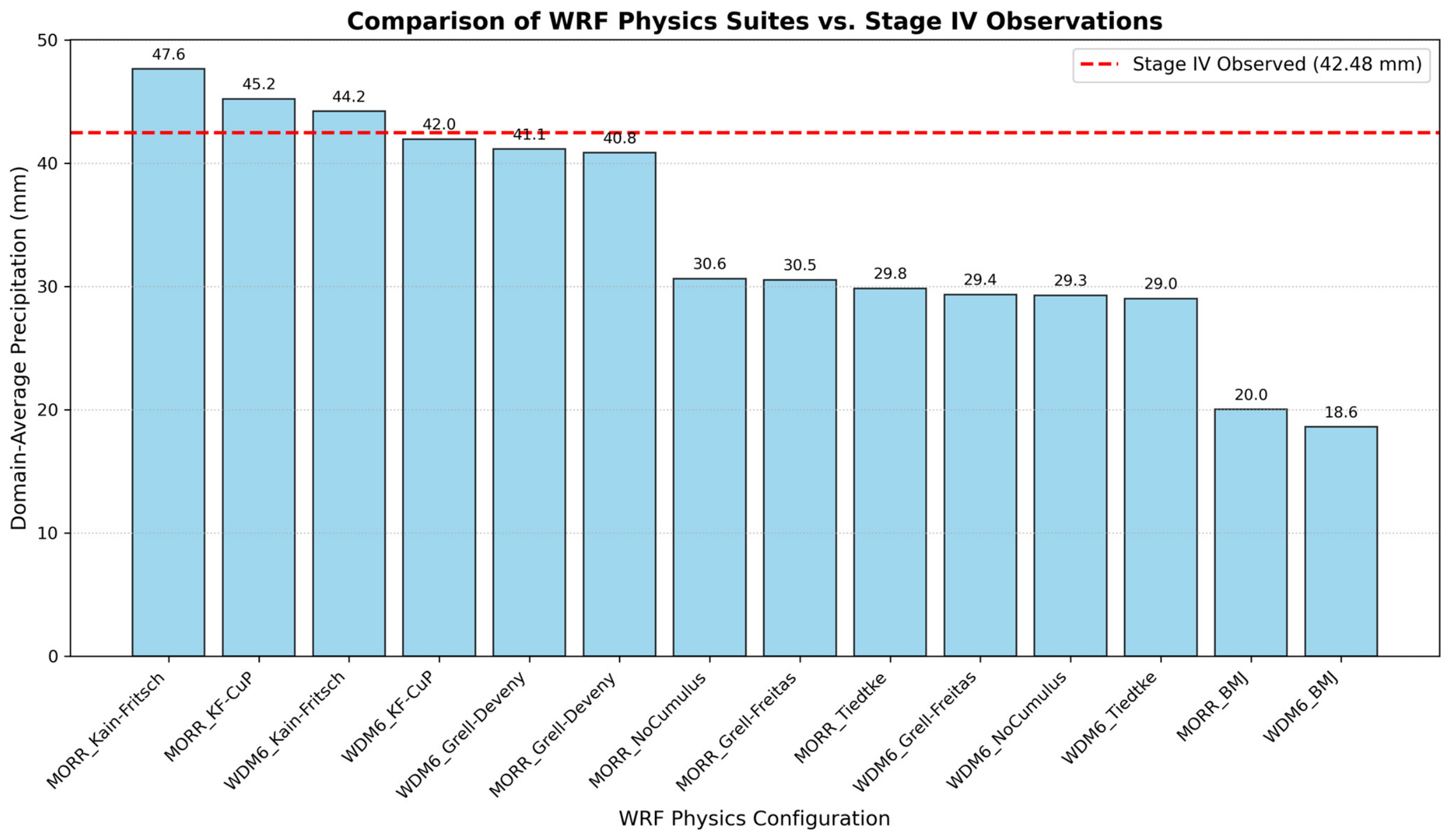
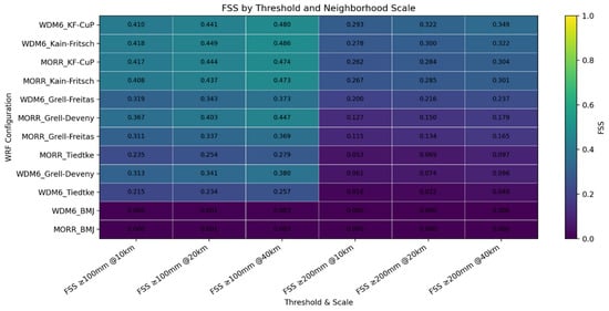
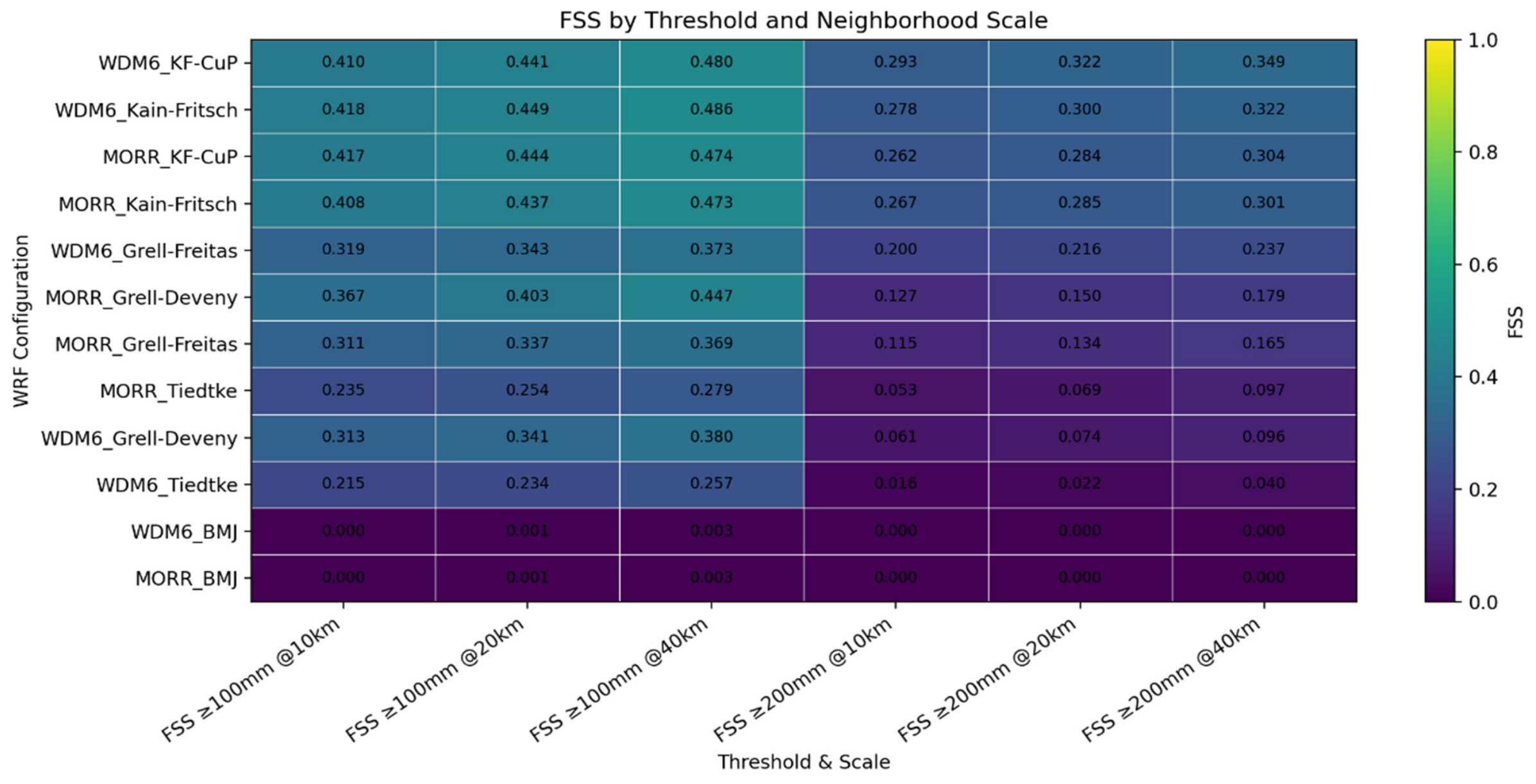
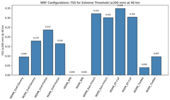
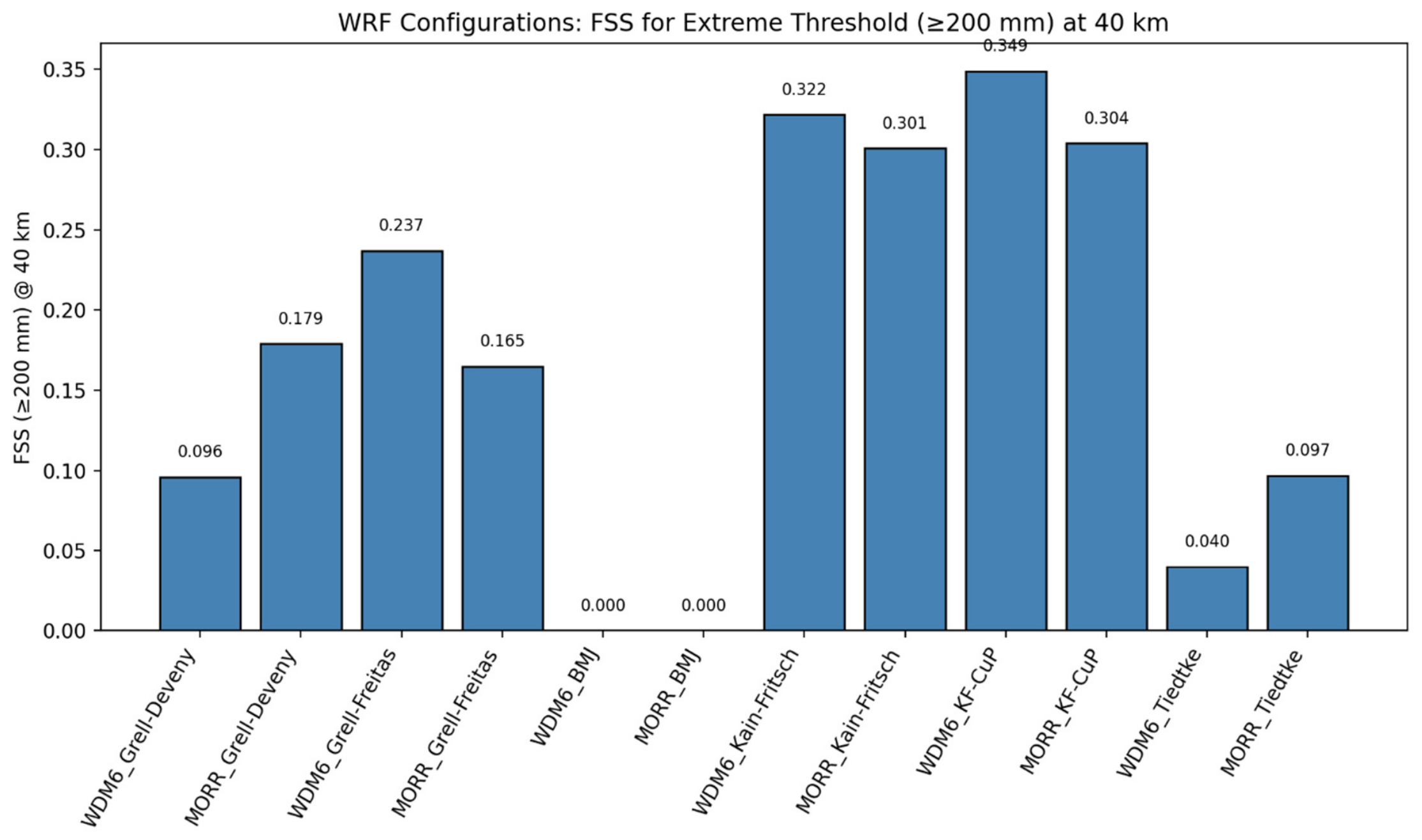
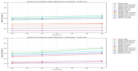
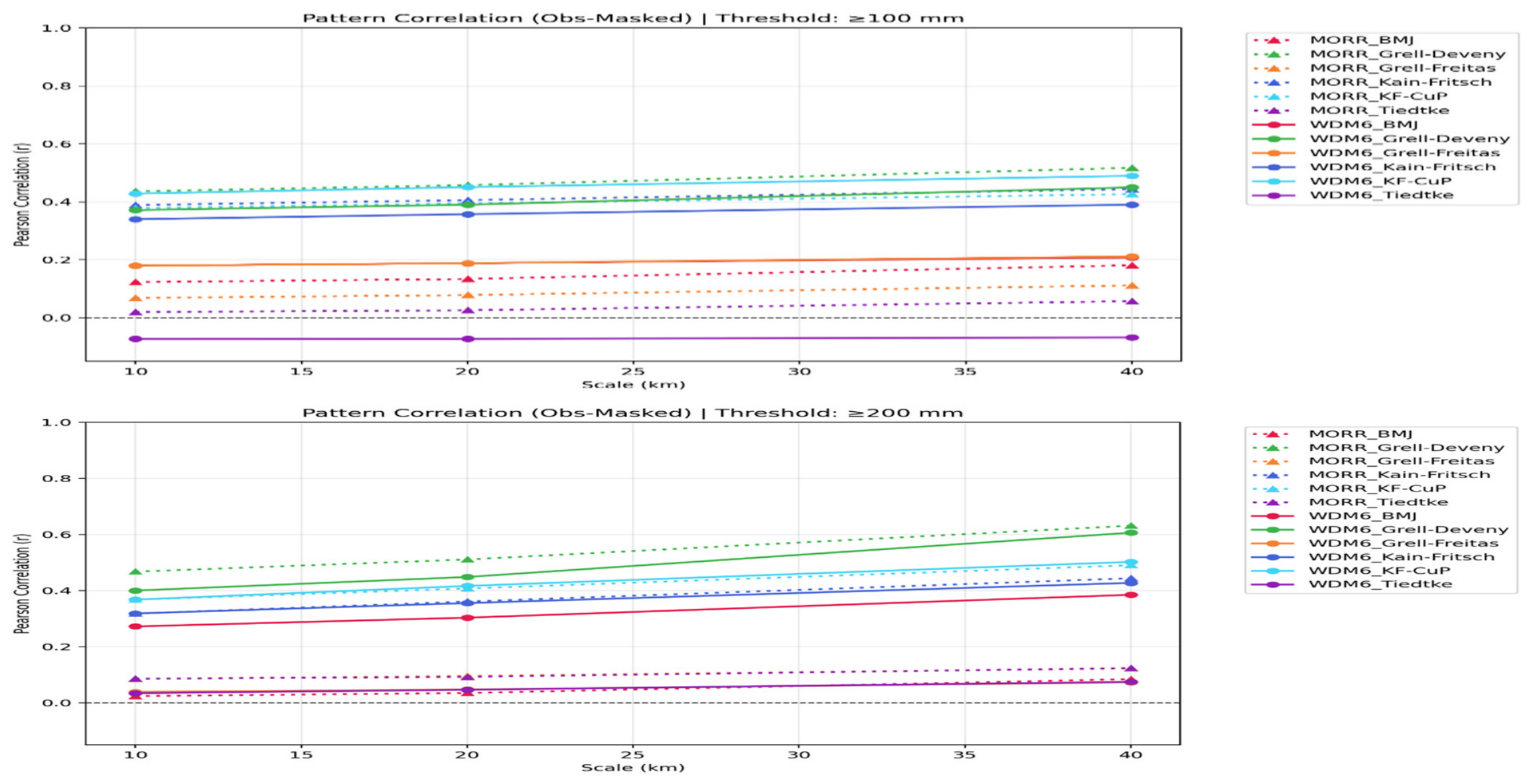
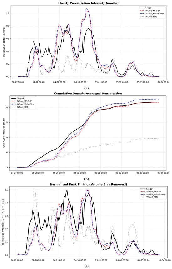
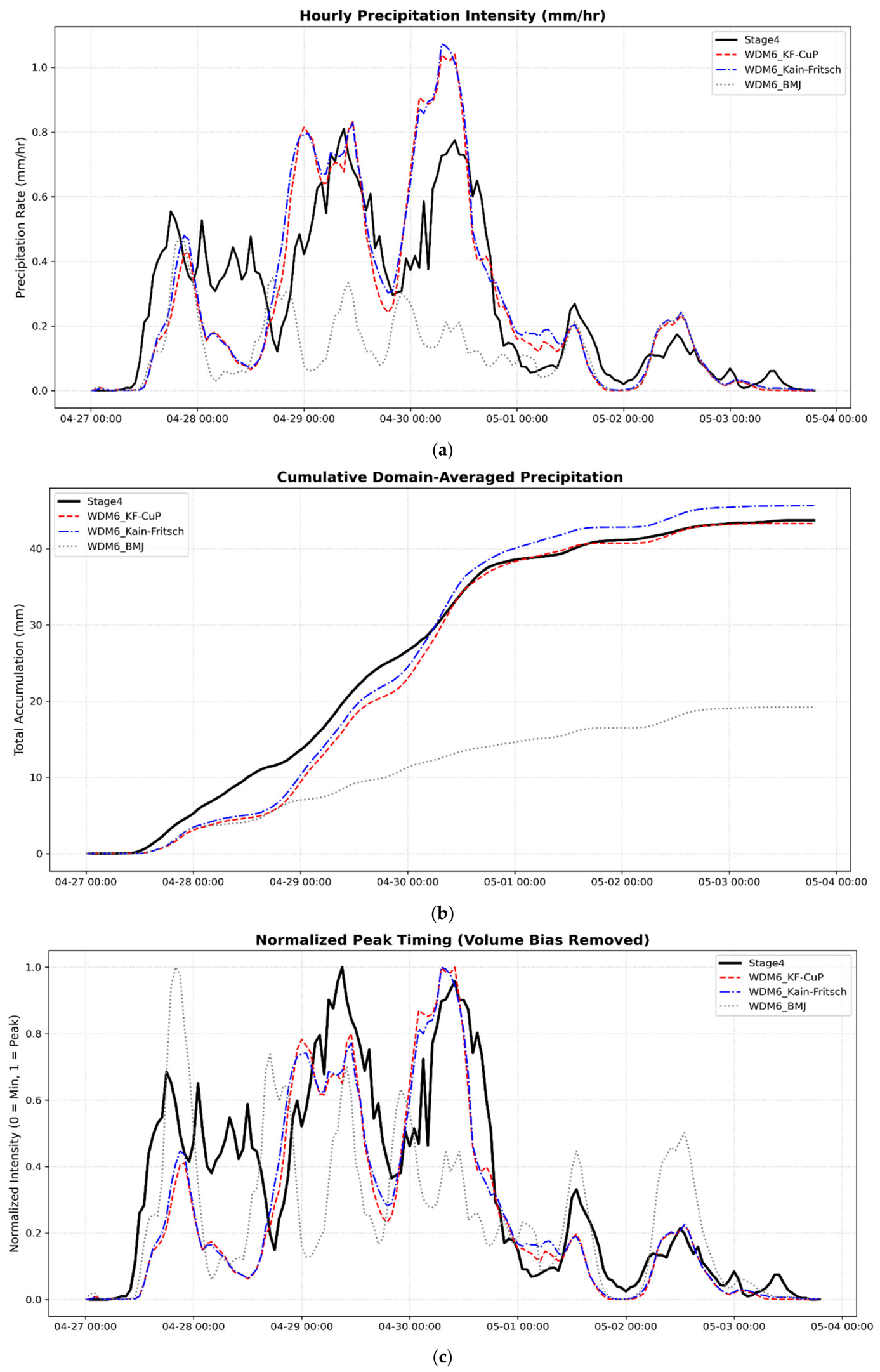
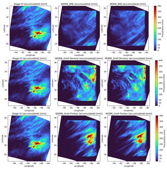
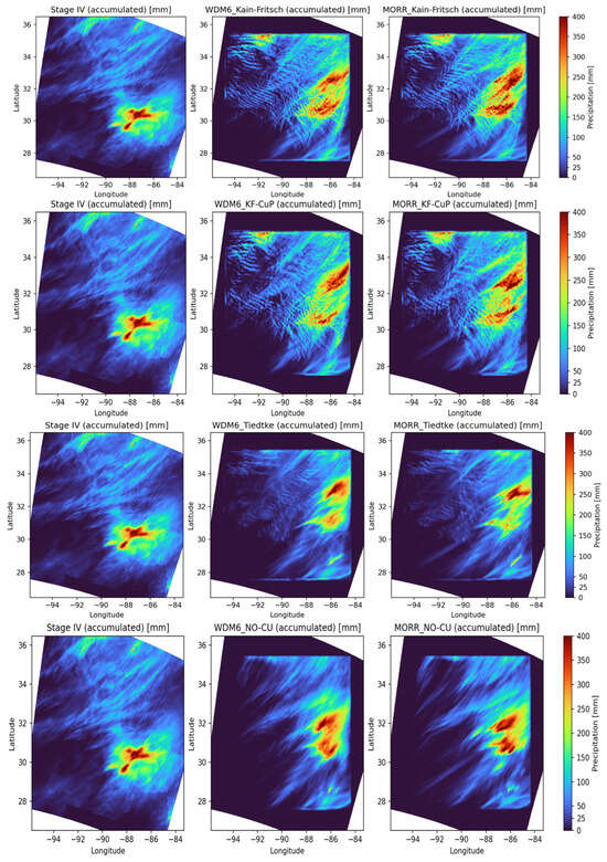
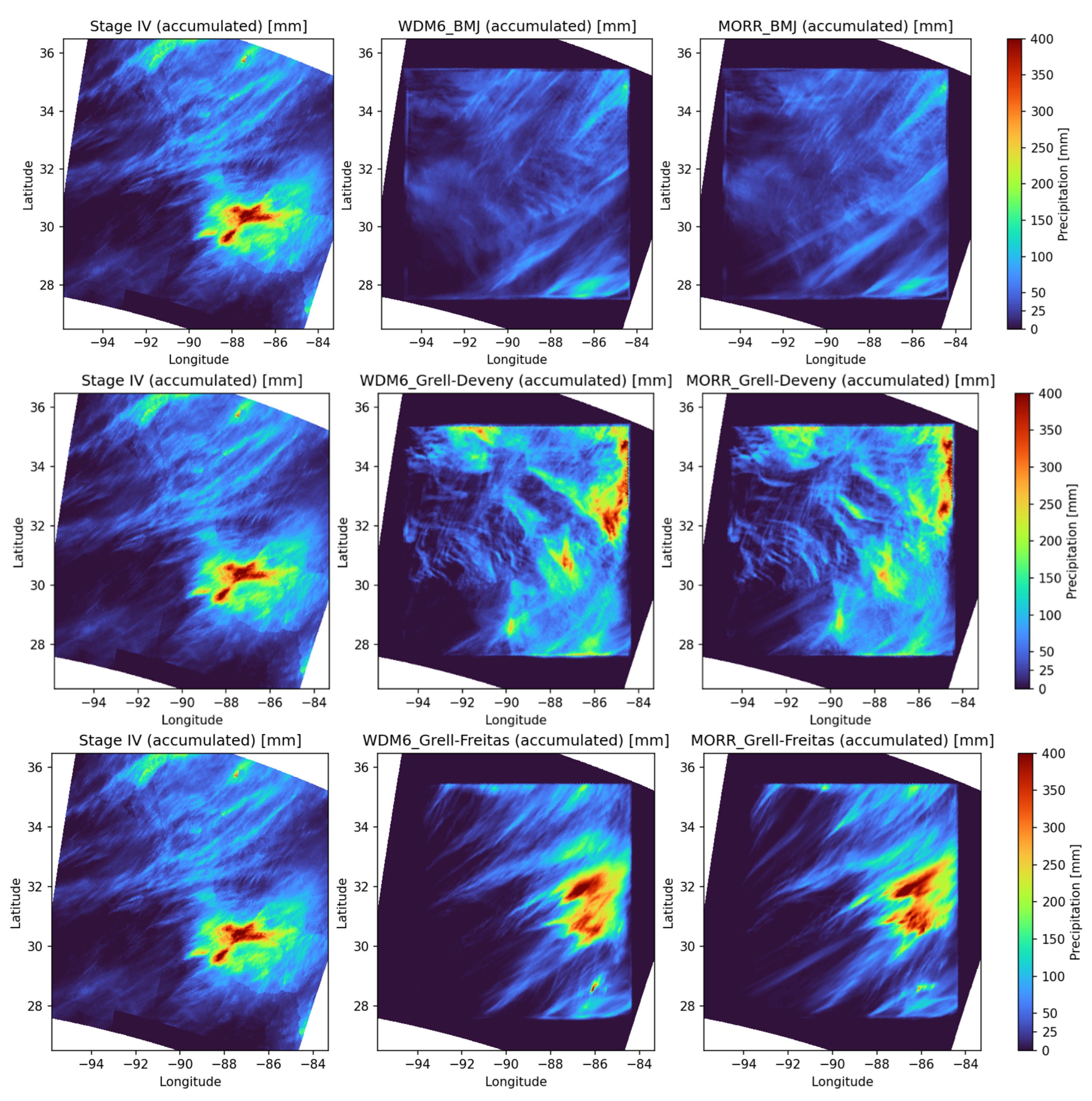
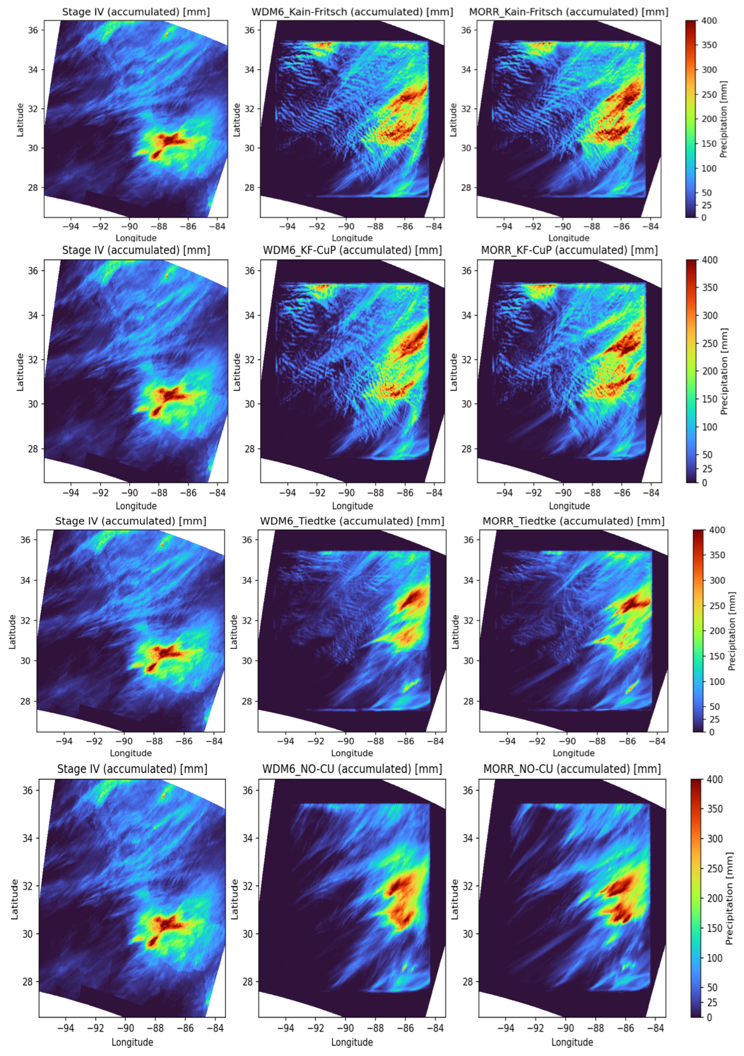
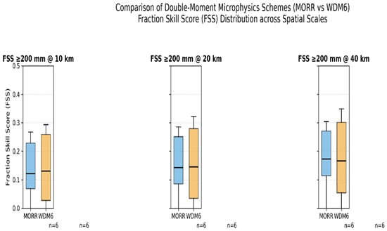
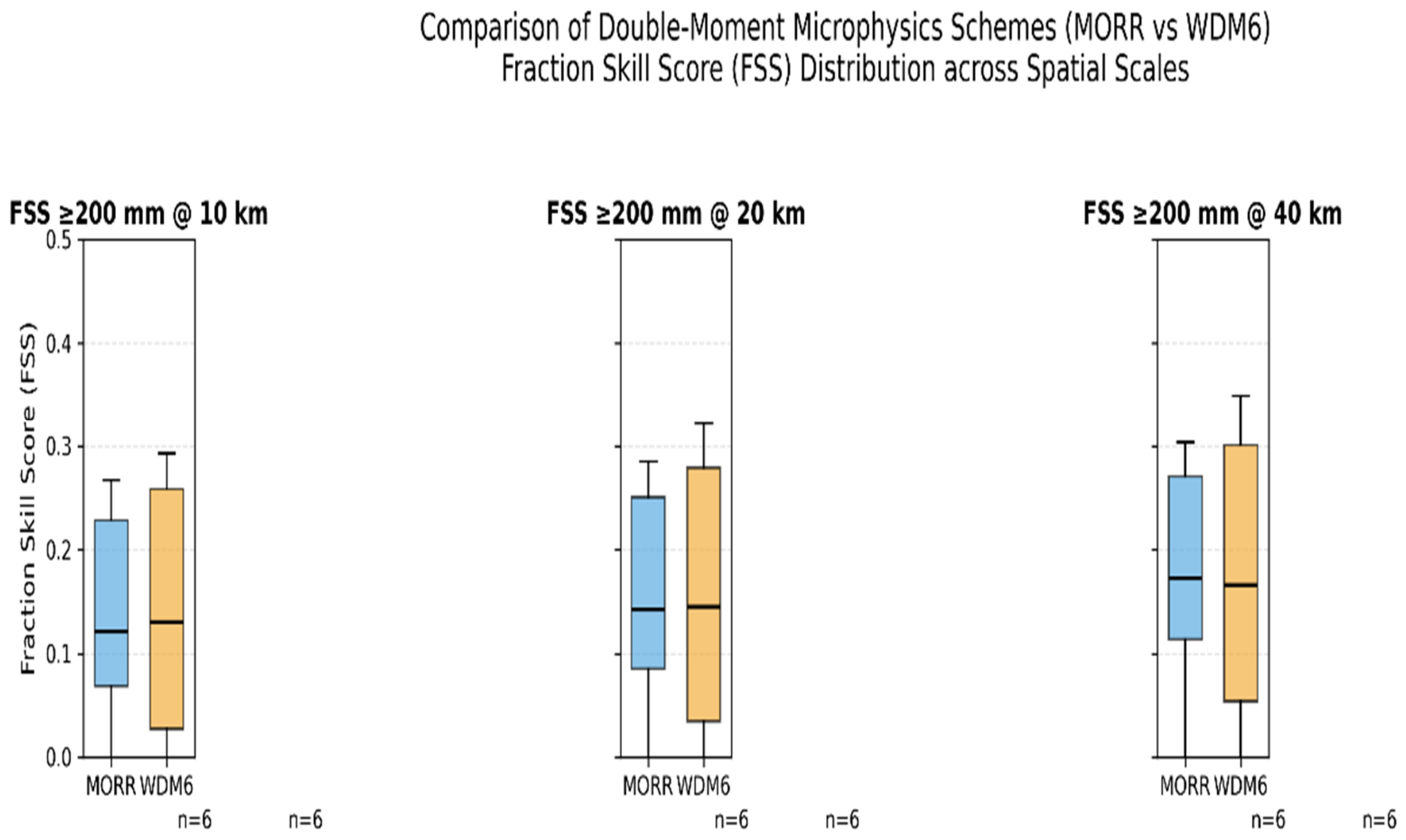
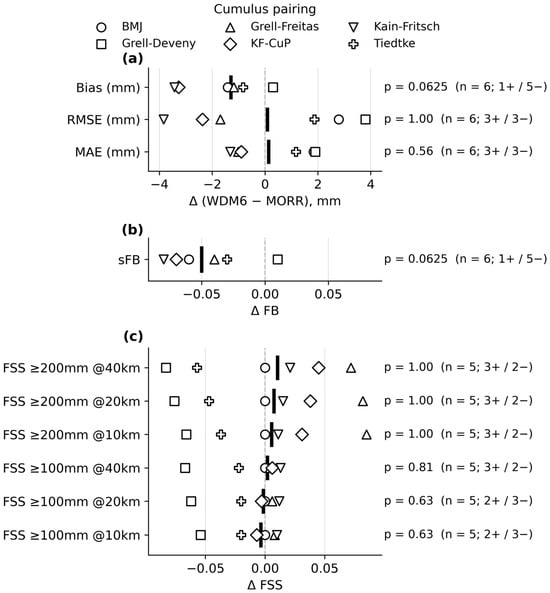
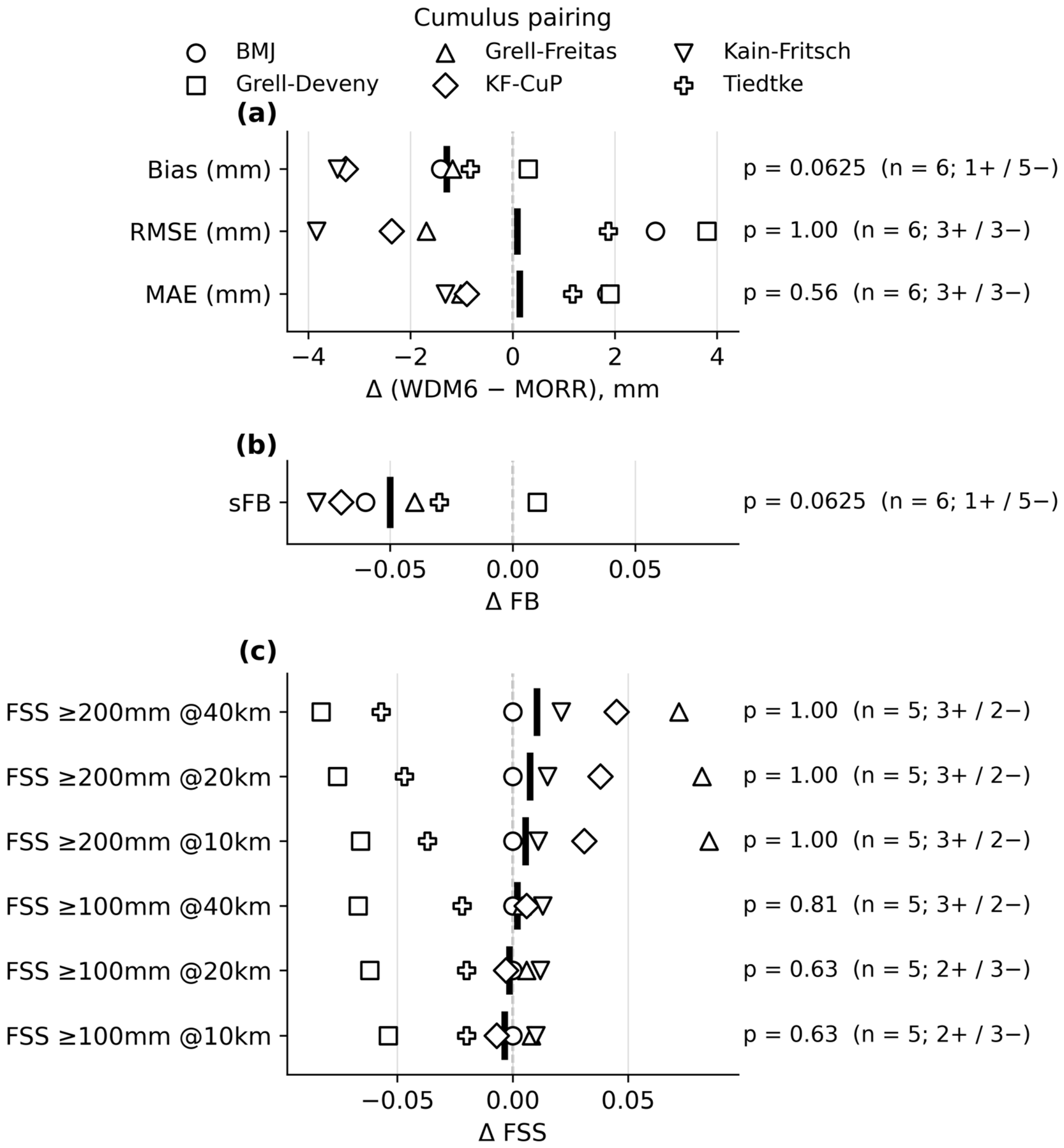
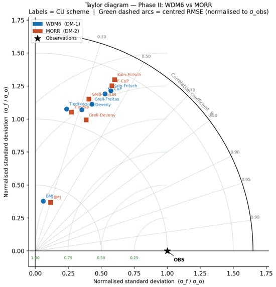
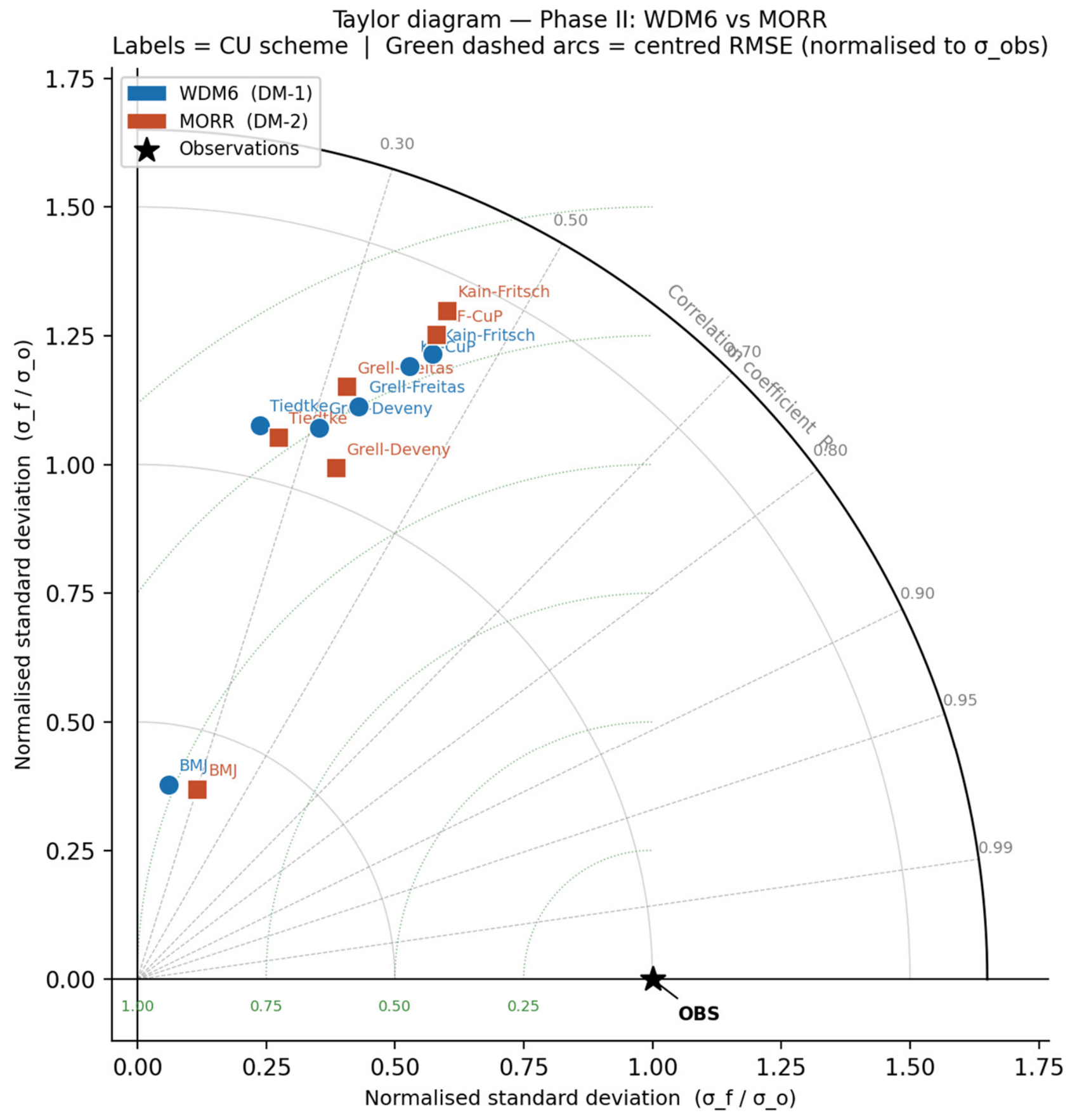
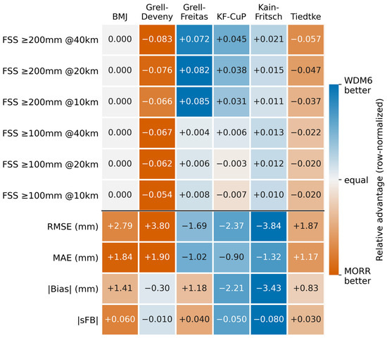
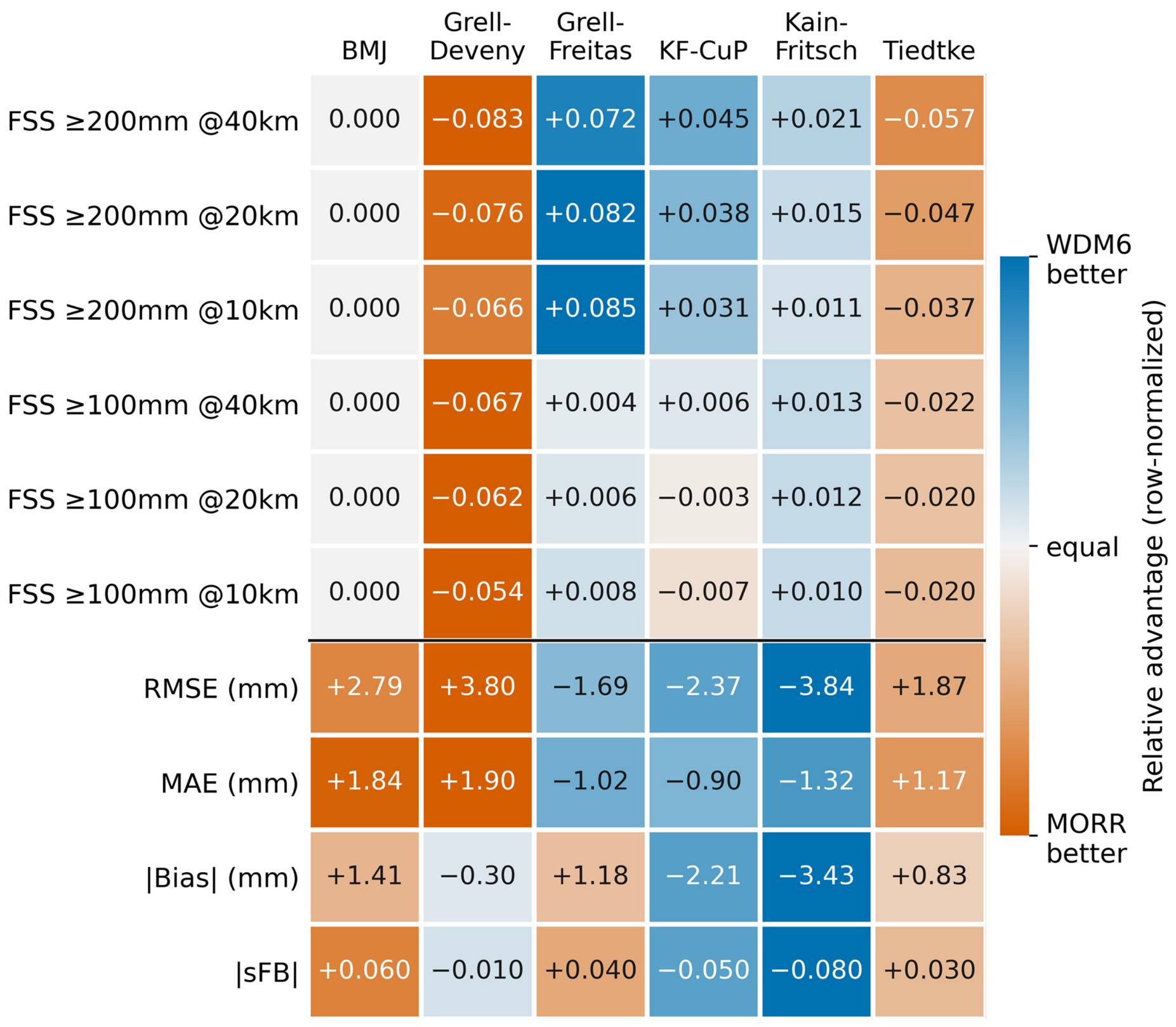
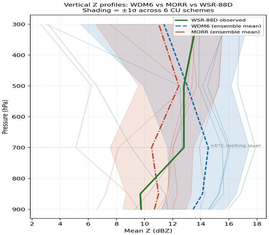
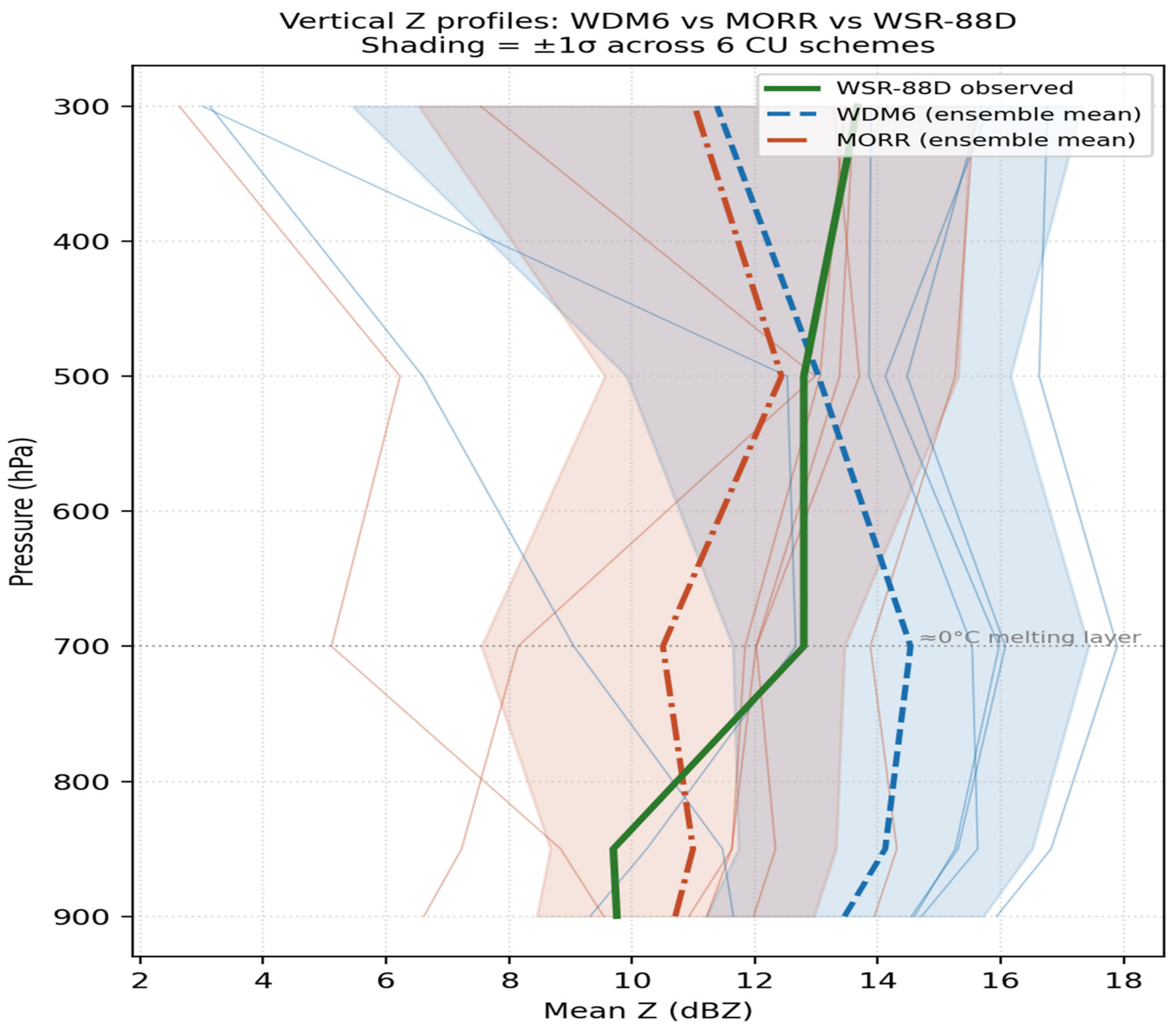
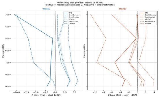
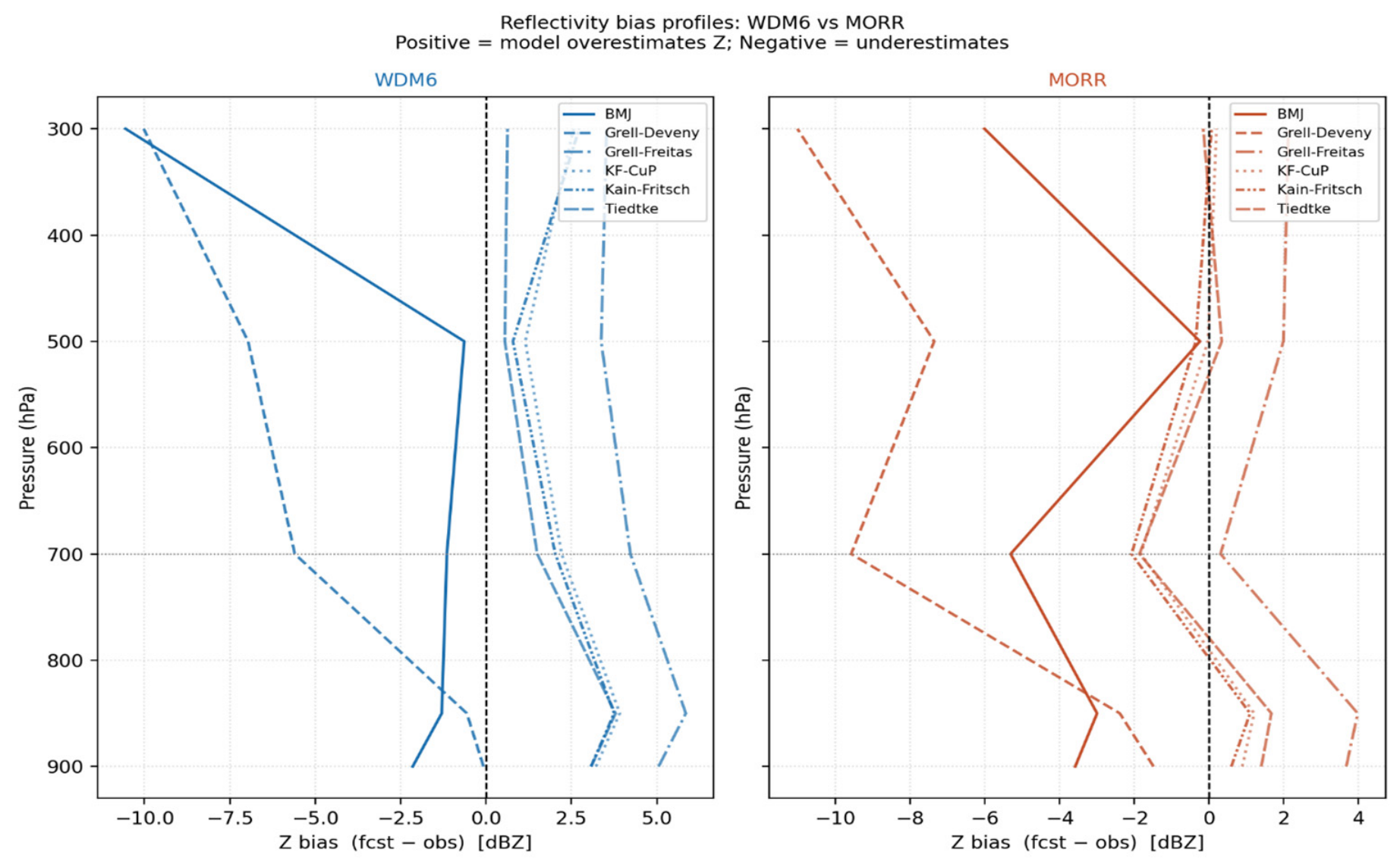
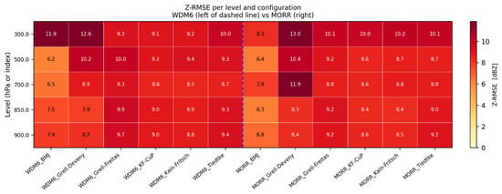
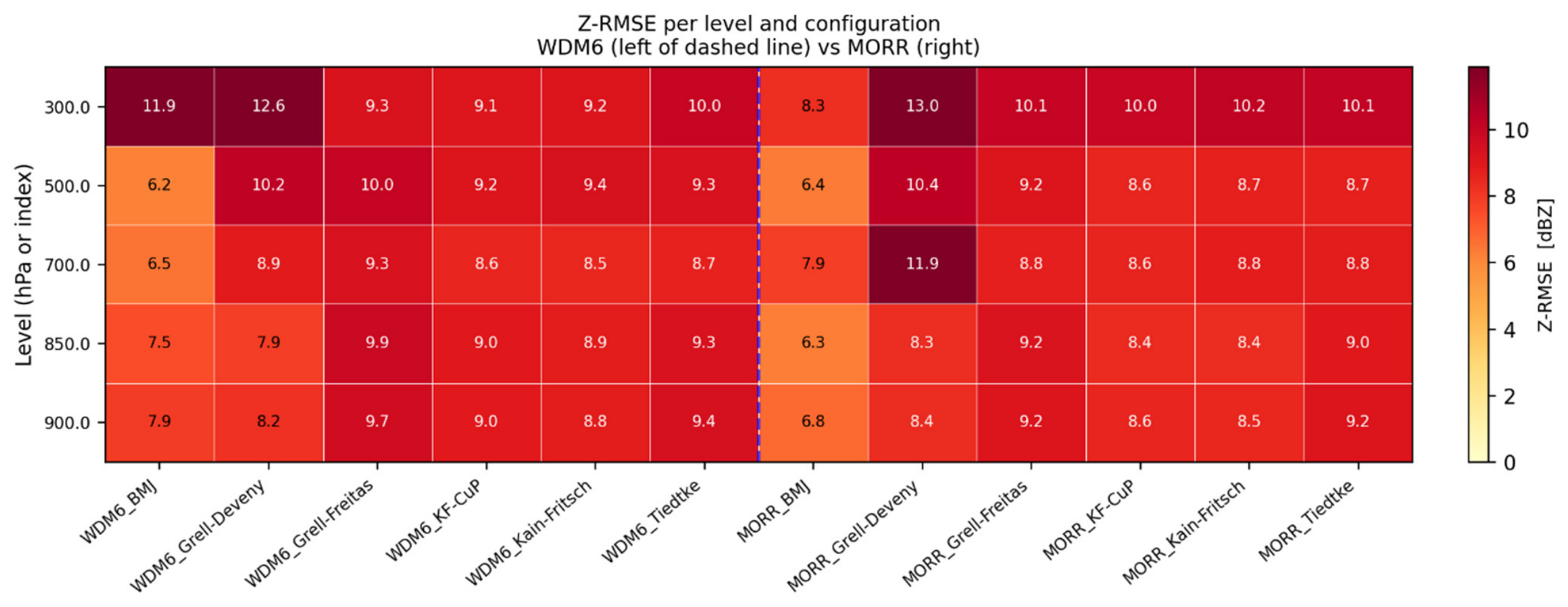
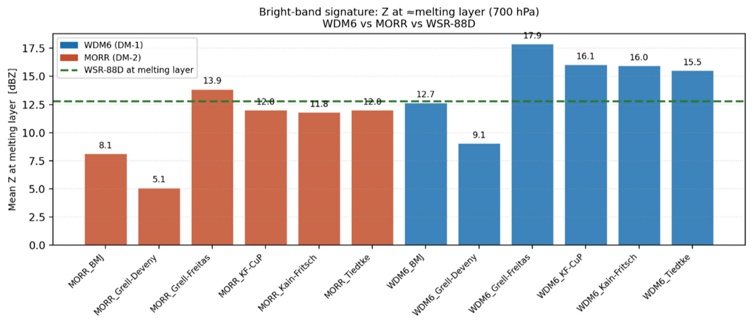

Disclaimer/Publisher’s Note: The statements, opinions and data contained in all publications are solely those of the individual author(s) and contributor(s) and not of MDPI and/or the editor(s). MDPI and/or the editor(s) disclaim responsibility for any injury to people or property resulting from any ideas, methods, instructions or products referred to in the content. |
© 2026 by the authors. Licensee MDPI, Basel, Switzerland. This article is an open access article distributed under the terms and conditions of the Creative Commons Attribution (CC BY) license.