


Abstract
Macroeconomic productivity is modeled as a Cobb–Douglas function of private and public R&D stocks in the recent literature. The slope parameters of a growth rate version may differ between countries and change over time and with circumstances. Using the method of functional coefficient regression, we show that human capital, GDP (per worker), services and defense R&D (both % GDP), lags of domestic and foreign private and public R&D, and lagged labor-augmenting technical change, all in growth rates, change the elasticities of productivity. The result is a panel dataset of regression coefficients representing elasticities of productivity for 21 rich countries. Eventually, the panel average of the productivity elasticities of domestic and foreign private R&D goes to constant values; elasticities of domestic public R&D go down slightly, whereas elasticities of foreign public R&D go up. This may contribute to an explanation of the productivity slowdown (mitigated by foreign public R&D) and why private R&D has been expanded relative to public R&D in recent years. Public R&D growth is associated with higher elasticities of domestic private and public R&D and lower ones of foreign private and public R&D and, therefore, offers a policy perspective.
1. Introduction
The literature on private and public R&D agrees on a positive link with productivity, with some exceptions of papers finding no effect of public R&D and some exceptions finding no effect of private R&D (See Soete et al., 2022; Ziesemer, 2021c, 2024c). These are extreme cases of the more general result that papers do not find numerically similar regression coefficients in similar approaches (see surveys of Hall et al., 2010; OECD, 2017; Ziesemer, 2021c).
If countries had similar elasticities of productivity of public and private R&D, we should expect similar private/public R&D stock or flow ratios. However, countries with higher incomes have not only higher private and public R&D (% GDP) but also relatively more private R&D (Coccia, 2010). Moreover, the private/public R&D ratio going from 1 to 3 during the period 1989–2019 for the USA (Ciaffi et al., 2024) may signal a shift of expected elasticities of productivity from public to private. These aspects can all be read as issues potentially questioning the assumption of fixed R&D elasticities of productivity, which are typically estimated as constant regression coefficients.
A productivity function is a condensed version of the view of how knowledge from R&D translates into productivity. Institutions of R&D may be separated from those of production that use the knowledge from R&D. The transfer of knowledge from R&D institutions to production organizations may, therefore, depend on the public and business environment, and it may change over time and across countries, leading to varying coefficients. One of these aspects may be technical change in the productivity function. Another one, emphasized in this paper, may be changes in the estimated parameters, which the literature has mostly assumed to be constant. An early exception is the suggestion of time-dependent parameters in Haavelmo’s (1954) ‘A Study in the theory of economic evolution’ on page 110.
In this paper, we try to find evidence for changes in R&D elasticities of productivity and the underlying causes or conditional associations. Moreover, as a by-product, we find indications of (in)efficiencies and/or technical change in the productivity function, which may be neutral as in the case of technical change in a Cobb–Douglas function or factor-biased in case of more general CES or VES productivity functions.
We test the effects on elasticities of productivity for several variables. Having more country-wide human capital in the country was suggested by Schultz (1964) as a source of more productive private and public R&D. Having higher or lower recent growth rates of GDP and past growth rates of GDP per worker may create changes in incentives explaining Coccia’s observation. As services (% GDP) have lower productivity growth rates (Herrendorf et al., 2014, Figure 6.10; Comin et al., 2025), countries with a higher share of services may have lower growth rates of productivity for the same R&D inputs at the macroeconomic level; this may be reflected in higher or lower macroeconomic R&D elasticities of productivity for private and public R&D when the share of services changes. More generally speaking, the regression coefficients may depend on disaggregation of the GDP with regard to the underlying factors and goods, and, therefore, their potential lack of constancy belongs to the class of aggregation problems in economics.
Moreover, the literature on defense R&D at times has doubted that it contributes to productivity (Mowery & Rosenberg, 1989). Similarly, for OECD panel data, Guellec and Van Pottelsberghe de la Potterie (2003) find a negative effect of defense R&D on business R&D, and “the defence component of government-performed research has a negative impact on business-funded R&D, civilian R&D has no impact” (Jaumotte & Pain, 2005, p. 38), which may reduce productivity growth. Fieldhouse and Mertens (2023) also do not find positive effects of US defense R&D. In contrast, Goel et al. (2008) find a higher rate of return for US defense compared to non-defense R&D, suggesting that the combination has an effect on the elasticities of production. Deleidi and Mazzucato (2021) find positive effects of US defense R&D on private R&D and GDP growth; Boysen-Hogrefe (2025) shows that using data only since 1985 leads to a crowding-out result. Both results together suggest changing coefficients. Moretti et al. (2025) find a positive effect of defense R&D on business R&D for a country industry year-level dataset for OECD countries and a firm year-level dataset for France. These diverse results suggest investigating how military expenditure on R&D affects the elasticities of productivity of public and private R&D.
For the analysis of changing elasticities of productivity, we combine the theoretical concept of Cobb–Douglas, CES, or VES functions for productivity depending on R&D variables and the empirical method of functional coefficient regression (Cai et al., 2000), which makes regression coefficients dependent on the arguments of the previous paragraph called functional coefficient series. This method leads to continuous shifts in the coefficients, and, therefore, fits the motivation given above better than other methods briefly discussed below because our motivation does not suggest threshold values or discontinuities captured as knots used in other methods.
A broader motivation can be based on the dissatisfaction with the use of Cobb–Douglas production functions, which are assumed to be identical across countries, years, or even sectors in the literature. Bernard and Jones (1996) have made the elasticities of production country-specific. The reason behind it is ‘the heterogeneity of goods that is produced in an economy’, leading to different theoretical and empirical convergence properties than under identical functions. Similarly, Temple (1999) suggests that ‘structural change leads naturally to questioning the relevance of aggregate production functions’. We will capture this argument using the share of services when analyzing the productivity function because what holds for production functions is likely to hold for productivity functions and R&D growth, which are at least as important for convergence and growth as production functions emphasized by Bernard and Jones (1996) and known since Denison (1962) and from others later. Durlauf et al. (2005) emphasize the existence of convergence clubs through the heterogeneity of the long-run growth rates based on human capital and technical change. In papers with two steady states, countries specialize either in manufacturing and services or in agriculture. Moreover, crucial parameters tend to depend on initial income, implying little mobility in the cross-country income distribution, as well as initial life expectancy and literacy. A more recent contribution using varying coefficients for production functions is T. Wang and Henderson (2022), suggesting local government expenditure on R&D as a driver of the elasticity of production of capital. For semi-parametric TFP regressions, Mamuneas et al. (2006) find parameter dependence for human capital on human capital and outward orientation. Lagged instead of initial income, human capital, services, and public R&D suggested by this literature appear as functional coefficient series below for regressions regarding labor-augmenting technical change and R&D variables. The heterogeneity of national systems of innovation and their changes over time (see Nelson, 1993; Castellacci & Archibugi, 2008; Castellacci & Natera, 2013) may also contribute to changing regression coefficients but require a separate paper because of the huge number of aspects discussed there; this could include policy incentives for special forms of financing start-ups (see Solodoha et al., 2023) and innovation efforts of other firms like SMEs, scale-ups, and large firms. Going to the next disaggregation level of production functions in manufacturing (Nelson, 1968) and agriculture (Eberhardt & Teal, 2013), we would get even more candidates for variables having an impact on the regression coefficients. More generally, in resorting to any other area of economics related to production functions, we could find more variables that change the coefficients. Not knowing them leads to cross-sectional dependence and omitted variable biases in connection with other methods for the analysis of heterogeneous panels; this phenomenon is called theory-openendness by Brock and Durlauf (2001). Eberhardt and Teal (2013) handle this econometric problem of unobserved variables by splitting the residuals of a production function equation into autoregressive common factors and remaining residual parts and allow for country-specific coefficients in the production function equation for agriculture. This leads to as many versions of constant regression coefficients as there are countries. In contrast, the method of functional coefficients is leaning on observable variables and has a different coefficient for each country-year combination or observation indexed it, leading to different versions of the regression coefficients, with Ti as the number of observations of country i. The common factor model is safe against biases, and it has constant coefficients that do not react to the observable functional series, whereas the functional regression method reacts to functional series but is not yet developed far enough to deal with biases from unit roots in regressors and functional series, endogeneity, missing fixed effects, and cross-section dependence jointly (see Section 3).
All authors mentioned in this paragraph avoid touching upon the everlasting issue of the impossibility of micro- or meso- to macro-aggregation of production functions.1 Given this impossibility, a macroeconomic production function is a mere assumption, which may lead to stable and constant coefficients only as long as there is not much structural change within or heterogeneity across countries. The variables emphasized above are exactly those which either bring structural change to growth paths (human capital, shift to services, and public R&D) or make it slower or faster (depending on the sign and size of coefficients of lagged dependent variables). Brock and Durlauf (2001) state that ‘identification of interesting data patterns … can both stimulate economic theory and suggest directions along which to engage in country-specific studies.’ When trying to do this and linking the results to these aspects of different strands of the literature, we may add intuition which goes beyond what is strictly shown by the regressions. This may be justified in the spirit of Brock and Durlauf (2001) again: ‘Empirical work always relies on judgment as well as formal procedures’.
Section 2 presents some basic theoretical production function concepts, which motivate empirical work and help in the economic interpretation of the results. Section 3 explains the method of functional coefficient regressions and its current econometric shortcomings. Section 4 describes the data, including their time trends and panel unit root analyses, as the method of functional coefficient regression as used requires stationarity (Cai et al., 2000). The results in Section 5 show how and which functional coefficient series, also called smoothing factors, have an impact on the regression coefficients when used separately and then put all effects together to see how regression coefficients or their combination for the direct and indirect effects of public R&D change over time. This produces many results with a method not often used in economics and not at all in the area of R&D and productivity. We summarize and interpret the results extensively in Section 5.3 for the relation between smoothing variables and regression coefficients of the productivity function as well as the effect of public on private R&D. Section 6 concludes with a summary of the overall results and provides suggestions for policy and future research.
2. Theoretical Model
Herzer (2022) and C. Y. Huang et al. (2025), in a theoretical endogenous growth paper, interpret the empirical literature on technical change at the country level as a Cobb–Douglas function of productivity depending on domestic business and government R&D stocks, denoted as B(ERD) and P(ublic), respectively. This is the standard interpretation found in earlier surveys (Hall et al., 2010; OECD, 2017). Van Elk et al. (2015, 2019) add aggregated foreign R&D, and Soete et al. (2020, 2022) add foreign private and public R&D separately and the lagged level of productivity. Equation (1a) states this assumption formally.
The first two terms are the direct effects of business and government R&D on productivity. X abbreviates other variables, such as foreign R&D variables and time trends mimicking technical change in the log version of the productivity function (1a). Optimal growth requires equal marginal products of private and public R&D (Ziesemer, 2021b), as formulated in (2a) for the Cobb–Douglas case:
Technical change would drop out in (2a) because T can be cancelled. Allowing for inefficiency in the sense of unequal marginal products, (2a) implies (2b) (a ‘hat’ indicating a percentage growth rate):
In case of efficiency, A = 1, and it is constant. Under inefficiency, A does not equal unity and may go to unity and thereby towards efficiency, or away from it, leading to increasing inefficiency. (2a) and (2b) are the theoretical basis to think of an indirect effect of public R&D: higher public R&D may be seen as an incentive for firms to invest in higher private R&D, and higher private R&D may be an incentive for governments to think of more public R&D. This can happen independently or through some policy coordination as known from OECD and EU recommendations and national policies. The model is a highly stylized formulation of these forms of coordination and adjustments.2 In particular, the growth rate of inefficiencies in the Cobb–Douglas case is as large as the differences in the growth rates of private and public R&D. Suppose instead that (1a) is replaced by the more general VES function3 (3).
D(t) and F(t) are exogenous technical change functions of time. A special case of (3) is the CES function for γ = δ = ε, with or without scale parameter θ = 1. If these parameters go to zero, we go to the Cobb–Douglas function (1a) again (requiring L’Hôpital’s theorem) with expressions for D(t) and F(t) multiplied and appearing as one term.
Equal marginal products of B and P from (3) lead to (4a), where the external derivative has dropped out:
δ[D(t)B(t)]δ−1D(t) = ε[F(t)P(t)]ε−1F(t)
Rewriting (4a) in terms of growth rates, we get (4b):
As D and F are exogenous by assumption, the sum of the last two terms is the intercept of the equation. If this sum is a positive growth rate, we call this BERD-biased technical change. In the special case of a Cobb–Douglas function, it is zero because we have dropped the idea of inefficiency A(t) through unequal marginal products, and F and D would drop out from (2b) if we had included them in (1a), where a log version can replace the corresponding sum by a time trend, and a growth rate version has them as a constant. The slope in (4b) depends on the VES parameters.
In the Cobb–Douglas model, α and β are constant elasticities of productivity. The major purpose of this paper is to go one step beyond this basic standard model to show that these elasticities may depend on the circumstances prevailing in the economy when trying to turn R&D experience into productivity. A second important aspect is that the unit elasticities in (2b) are unlikely to be fulfilled. (4b) then offers a more realistic alternative; the CD version can be remarkably close to these, though. We will relate the empirical works introduced next to these functions without adhering strictly to one of them or trying to clarify which is more realistic. The reason for this is that the central hypothesis of this paper is that the regression coefficients of a growth rate version of (1a) and (1b) below and the linear Equation (4b) or (5) below do not have constant regression coefficients but rather changing ones depending on the functional coefficient series introduced above. In order to indicate the relevance of this, we relate the results to the development of the public–private R&D ratio and the productivity slowdown without a comprehensive treatment of these issues.
3. Empirical Methodology
Functional coefficient regression is a semi-parametric method. Regression coefficients a and b in Y = a + bX + u are made dependent on variables Z called functional coefficient series, leading to functions a(Z), b(Z). These functions are local polynomials of degree l, (or other nonlinear functions)4 in the variables Z, where cjl is the l-th derivative of the j-th coefficient, which could also include the term . The polynomials are Taylor series approximations of the Z variables (Cai et al., 2000; Fan & Zhang, 2000). The variables Z are, for example, current or lagged regressors: Z = X, X(−1) (Chen & Tsay, 1993), time trends, Z = t (Hastie & Tibshirani, 1993; Cai, 2003), lagged dependent variables, Z = Y(−1) (J. Z. Huang & Shen, 2004), or other lagged variables, Z = V(−1) (J. Z. Huang & Shen, 2004). Variables Z have to be determined according to economic context based on a priori knowledge of the researcher. The economic literature has not applied this method very often, and if so, outside the area of R&D and technical change.5 Polynomials a(Z) and b(Z)—where b, in case of several regressors, and Z can be vectors—are then inserted, resulting in Y = a(Z) + b(Z)X + u. Functional coefficient series are weighted with kernel functions. The estimation method then is penalized least squares in combination with non-parametric procedures to find kernel functions, which balance low bias with high variance under a small bandwidth and high bias with low variance under a large bandwidth (Ullah & Pagan, 1999). We should choose the Taylor approximation with the highest degree that still yields a smooth curve (Chen & Tsay, 1993).6 Estimation bias and confidence intervals are found by way of comparison with using two (or more) additional degrees of the Taylor approximation (Fan & Zhang, 2000). Using a lower degree of Taylor approximation than the highest, resulting in a smooth curve, therefore, would lead to a larger bias. The rules for smooth curves and bias limit the space for sensitivity analysis. Bandwidths are automatically chosen under CV (cross-validation favored in literature). Higher polynomial degrees would be non-smooth and should not be chosen, and lower ones lead to a higher bias (perhaps also simpler benchmark models); both are, therefore, not interesting comparisons. The Epanechnikov kernel is in the middle of the range of alternatives regarding least and most smooth and, therefore, is the default. It is clear that most observations are in the middle of the range of the figures, and excluding the extreme ones leads to curtailing the curves at the end in the spirit of estimation of repeated cross-sections and, therefore, the interpretation focuses on the middle of the range.
Statistically competing models are linear autoregressive models with lag p, ar(p), and threshold models (transition, smooth) (see Cai et al., 2000), and it is a matter of testing which work better. Our results, therefore, should not be misunderstood as criticism of (v)ar, threshold, or spline models. We do not compare our results to these alternatives because they are related to different economic research questions than the productivity–R&D link. Thresholds and, to some extent, lags are statistical steps, whereas the functional coefficient series Z also brings more economics into the analysis. Similarly, more traditional methods, such as rolling windows and slope dummies, do not include reasons for the coefficient changes, such as the functional series Z; the same holds for spline-based nonlinear models. They can be used when the functional series Z are not of interest, and other purposes are more important; perhaps in connection with keeping analyses simple for case-specific reasons. By implication, we do not claim that functional coefficient regression is superior in general; we prefer it here, and for other research questions, other methods may be more suitable. Several of these models are compared in Chen and Tsay (1993), Cai et al. (2000), and Fan and Zhang (2008) but not applied to the area of R&D.
We estimate the equations in growth rates as the data described below have unit roots. The production function (1a), in growth rates with c(i) as regression coefficients, is (1b):
DLT = C(1) + C(2)DLT(−1) + C(3)DLB + C(4)DLP + C(5)DLB* + C(6)DLP*
D indicates a difference. L is a natural logarithm. T is the labor-augmenting technology level, B(ERD) is the private R&D stock, P is the public R&D stock, and a ‘*’ indicates the corresponding variables of foreign countries. The intercept C(1) can be interpreted as an exogenous part of exogenous technical change.
The regression coefficients of (1b) are estimated as functions of growth rates of human capital, log(hc/hc(−5)), lagged GDP per worker in the labor force, d(log(gdp(−5)/(lf(−5)))), current share of services in GDP, d(log(srvy)), and lags of defense R&D as share of GDP, d(log(0.00000001 + defrdy(−5))), and they are all motivated in the introduction. Moreover, coefficients may be functions of the lags of variables in (1b), dlth07(−2), dlberdst(−5), and dlpubst(−3),7 as suggested by the FAR model in Cai et al. (2000) and others.8 As a consequence, the elasticities in (1b) will not be constant, but they will vary with the state of these variables and change over time. Again, l or log indicates a natural logarithm. d indicates a difference chosen to ensure stationarity of the variables as required by Cai et al. (2000). Without it, variables may have unit roots.
Juhl (2005) argues that results with nonstationary variables still make sense if the residuals are stationary, implying cointegration. This can easily be specified but is not guaranteed empirically (Y. Wang & Phillips, 2025). Tu and Wang (2022) point out that cointegration testing for functional coefficient regression is just in its infancy. Therefore, we use only stationary variables. Cai et al. (2009) analyze the case of nonstationary functional coefficient series Z in terms of statistical theory. Their two-step procedure to include variables with unit roots is not yet integrated in Eviews14.9 Using cointegrating relations of nonstationary variables rather than stationary variables may change the results in future research.
Another econometric issue is endogeneity,10 which is also not yet addressed in the EViews14 tool for functional coefficient regression and the corresponding manual chapter, and in the underlying article by Cai et al. (2000). Cai et al. (2015) deal with endogeneity, but EViews has not yet integrated this; this might indicate that the econometric development is not yet sufficiently advanced to allow for the development of package tools. Our results are, therefore, based on the hope that a potential endogeneity bias is small (see Nakamura & Nakamura, 1998) and that having functional coefficients is quantitatively more important. This makes the results preliminary, and the exact numbers should be taken with a grain of salt; what matters is that regression coefficients are not constant. Future research may lead to modifications of the exact numbers but most likely not to constancy of coefficients. Nevertheless, we provide a lot of information in regard to functional coefficient series, which sometimes are called factors or smoothing variables (Cai et al., 2015). It should be noted that the definition of bias in comparison with polynomials two degrees higher used in functional coefficient analysis is different from the standard endogeneity bias of correlation between residuals and regressors. Correlation of R&D variables is most obvious during financial crises where they fall (with the exception of countries with countercyclical public R&D policy). In better and normal times, we consider R&D a matter of long-term planning which is unlikely to react to residuals. The endogeneity considerations of Cai et al. (2015) will help us in the future to test for this and take it into account in the estimation. In the words of two reviewers, ‘many of the reported relationships should be interpreted more cautiously as conditional associations rather than causal effects’. Causal formulations such as “increases,” “reduces,” “leads to,” and “enhances” are typically used in economic interpretations, adding some economic intuition below; readers worrying about the causal formulations should feel free to replace them by “is associated with,” where appropriate.
Sun et al. (2009) have added individual effects to the regression equation of interest. This introduces a second source for bias. The literature has then used several ways of eliminating the fixed effects, such as differencing and other methods (Rodriguez-Poo & Soberon, 2014; Henderson et al., 2026). This leads to a lower bias with a higher variance. To deal with the higher variance, several methods have been proposed in the literature. These methods seemingly have not yet converged to a standard tool and, therefore, are not yet included in Eviews14. A critical question for future research, therefore, is whether fixed effects lead to strongly different intercepts compared to those that we get with intercepts dependent on the functional series and thereby differing for each country-year observation. In the growth literature, fixed effects are most relevant for Africa and Latin America (Brock & Durlauf, 2001), which are not part of our sample, but weaker effects may also change our results if unobservable variables are not strongly correlated with our functional series.
For cross-sectional dependence in the functional coefficient models used here, there are only two closely related papers (Zhao et al., 2025; Cai et al., 2022) with asymptotic results; nothing like this is integrated into Eviews14 as it is in its infancy and has no small sample results yet. For our sample with T > N, a SURE mechanism would be the first suggestion from standard econometrics. In connection with endogeneity and fixed effects, one would then think of 3SLS and GMM-HAC as methods that should be related to functional coefficient regression; common factors could be used for shorter panels. This is econometric work to be done in the future. Ultimately, unit roots in regressors and functional series, fixed effects, endogeneity, and common factors need to be integrated in econometric packages jointly, whereas their treatment currently is handled separately in several articles on functional coefficient regressions.
Logs and lags of the functional series changing coefficients have been found by way of experimentation. We include all smoothing series for which we can reject the hypothesis of constant coefficients. In the first phase, we use each series alone and test that coefficients are not constant for several lags, trying lags 1 to 6 and, in some cases, beyond; otherwise, variables could seem to produce smooth results, which are actually caused only by covariates used simultaneously. For every given value of a functional series, we implicitly have a cross-sectional regression estimating the regression coefficients. Then, the method shifts to the next value and estimates the regression coefficients again, which should generate similar values in order to get a smooth series of the regression coefficients. In the second phase, we have used the previously significant variables jointly. Testing for linear, quadratic, and cubic approximation, and in some cases polynomial degree 4 and higher (see notes to figures and tables), we find the highest degree yielding a smooth curve and the lowest bias.
The effect of public on private R&D from (4b) is as in (5):
DLB = C(7) + C(8)DLP
The constant can be interpreted as the growth rate of the BERD bias indicator in (4b), as inefficiency growth as in (2b), or as a combination of both because they cannot be distinguished empirically. The symbols are explained above. We have experimented with the same functional coefficient series as for (1b). We find smoothing effects for five-year changes of human capital, log(hc/hc(−5)), lags of services (% GDP), d(log(srvy(−3))), d(log(srvy(−4))), d(log(srvy(−5))), defense R&D, d(log(0.00000001 + defrdy(−2))), dlfberdst(−3), the average of GDP growth rates of the last four years, sumg4 (using degree 4), and lags of variables in (5), which are here only dlberdst(−2).
For (1b) and (5), testing for constant coefficients (defined as not varying with functional series) may run into the problem of ‘attempt to raise a negative number to a non-integer power’. In these cases, we try to avoid the problem using a polynomial of a lower degree. Later, when calculating the coefficients C(1)–C(8), we go back to the smooth curve from the polynomial with the highest degree. The estimation bias is calculated through comparison with a polynomial of (at least) two degrees more, on which the confidence intervals are also based, which test whether coefficients are different from zero; simultaneous confidence bands are based on bootstrapping (Fan & Zhang, 2000).
For public R&D, the direct effect then is c(4), and the indirect effect is c(3)*c(8) from (1b) and (5). The total effect of a one percent change in public R&D is then c(4)+ c(3)*c(8). This simple model ignores all impacts and feedback on and from foreign R&D and feedback from private on public R&D, as it was considered using vector error correction models by Soete et al. (2020, 2022) and Ziesemer (2021b), which is more in the spirit of the ar(p) models mentioned above. The method of functional regression coefficients is a single-equation method serving well the purpose of this paper, but it is not a system method.
Finally, the use of services and human capital may remind readers of the productivity decomposition analysis in regard to sectors and factors (see Cantner et al., 2018). The analysis writes the growth rate of productivity, g, as the sum of weighted growth rates of sectors or factors i: . The weights may be, for example, cost shares, expenditure or value-added shares, or market sales shares. Taking growth rates as log differences of variables Y and Xi and removing the differences, the equation can be written as . The delog operation leads to the Cobb–Douglas function . Instead of a macroeconomic productivity function (1a), the productivity decomposition analysis uses disaggregated variables of sectors or factors and related parameters as a starting point and then differentiates the growth rate version and fills it with data. This produces a lot of information for many sectors or factors if the required datasets for the research questions are available. The functional coefficient regression instead uses arguments to explain the coefficients of a macroeconomic productivity function regression. For both methods, the explanation is mostly intuitive based on background knowledge regarding aggregation problems for quantities, prices, production, and welfare functions, and the problems connecting micro-, meso-, and macroeconomic relations as well as panel data (Pesaran, 2015; ch. 32).
As regression output for functional coefficient regression in Eviews14 does not give any results known as model selection criteria, we cannot compare our results to similar ones, especially smaller ones, and exclude the possibility that alternative or additional functional series generate better models. However, future research can try to find additional variables as usual in empirical econometrics.
4. Data
We use a dataset similar to that of Van Elk et al. (2015, 2019) and Soete et al. (2022) (extended later to 2017) and extend it to 2021 for R&D data for all 44 countries of OECD MSTI, where explanations are given in detail in Ziesemer (2026). Moreover, labor-augmented technical change data from Ziesemer (2023) are updated until 2019; here, we use the one based on a CES production function under an elasticity of substitution of 0.7. These data are explained in detail in Ziesemer (2023, 2026). The required human capital data are taken from PWT 10.01; they are weighted-average data from years of schooling in Barro-Lee.com, defined on a scale from 1 to 5. Data for GDP, labor force, and services (% GDP) are taken from World Development Indicators.11 R&D expenditures on defense are taken from OECD MSTI. All data are measured ex post, and, therefore, are supply- and demand-driven.
The data are divided into two subsamples. For the richer countries, there are longer data series. For the emerging economies, there are shorter data series. In this paper, we only use the longer data series for the richer 21 countries: Australia, Austria, Belgium, Canada, Switzerland, Germany, Denmark, Spain, Finland, France, the United Kingdom, Ireland, Iceland, Italy, Japan, Netherlands, Norway, New Zealand, Portugal, Sweden, and the United States.
Table 1 shows the standard information of the data; the histograms of the functional variable series are plotted in Appendix A: The human capital value is defined as between 1 and 5, and, therefore, all values and their logs are positive. We also add panel unit root tests. We mostly use Pesaran’s CIPS tests, which use a weighted statistic of country-specific ADF tests. In some cases, we add the Bai–Ng test in the Ahn and Horenstein (2013) manner to find common factors and test for their unit roots in addition to those in the residuals. When there is too low a number of observations for using these tests, we use those assuming no cross-section dependence. After all, for foreign private R&D, the results from the preferred Bai–Ng test support stationarity; the growth rate of foreign public R&D has a probability of unit root in the residuals of 0.21. Here, we decide to stick to the theoretical model and assume that it is stationary. These probabilities do not justify jumping out of the model that is under consideration, also because these are only univariate tests that do not take into account interactions with other variables (Jusélius, 2006). Unfortunately, tests that reverse the hypotheses, like KPSS, are not available for cross-sectional dependence; they can lead to the situation that the hypotheses of ‘unit root’ or ‘no unit root’ are both rejected or both not rejected. Moreover, in the debates between CIPS and Bai–Ng PANIC, the various parts of the literature are quite critical of each other. Therefore, we are a bit more lenient in regard to significance levels to deal with this situation because there is also a possibility of over-rejection error, especially in the case of small numbers of observations. Where the log levels have a unit root, we use their difference in the estimation below. The differenced variables are growth rates with mostly low probabilities for unit roots. Overall, they have a strong variation in terms of difference between maximum and minimum, and in terms of standard deviations.
Table 1.
Data description for a sample of 21 rich countries with long data series.
In the pre-column, the variables are presented immediately as estimated constant and time trend. All growth rates have a negative trend in the sample data, except for defense R&D, which has no trend. Therefore, we will formulate most interpretations below for falling growth rates going from right to left when reading the figures below. This leaves the cross-section interpretation to the reader to save space. The growth rates for domestic and foreign public R&D are more negative than those for all other variables in Table 1, a fact recently discussed by Archibugi and Filippetti (2018) and resumed below.
5. Results
In addition to the variables in Table 1, we have also tested ‘Internet per head of the population’ in several variants of log(1 + intpopxhc) or modifications; they do not yield smooth results for the long, rich sample for any lag. Therefore, we do not use an internet variable.
In Figure A1, Figure A2, Figure A3, Figure A4, Figure A5, Figure A6, Figure A7, Figure A8, Figure A9, Figure A10, Figure A11, Figure A12, Figure A13, Figure A14 and Figure A15 (see Appendix B coefficient series), the functional coefficient series in the Taylor approximation polynomial are listed below the graphs. The graphs show the impact of only one of the functional coefficient series. Adding the other functional coefficient series for the test of constant coefficients leads more often than not to the warning ‘attempt to raise a negative number to a non-integer power’ and thereby no results. From the perspective of an economic interpretation, it is clear then that the effects in the figures below stem from one variable only and not from including other functional coefficient series from Table 1 with lags. When we want to calculate the coefficients of (1b) later, we use all functional coefficient series simultaneously, but we do not need the test for constant coefficients again. To show all the impacts, we inevitably get as many figures for the productivity function (1b) as we have functional coefficient series, with each one graph per regression coefficient in (1b). We only discuss the main impacts; at the very left or very right of the graphs, there are often results based on small numbers of observations. As most observations are in the middle of the range, we also discuss the effects around the mean and median shown in Table 1.
5.1. Partial Effects of Functional Coefficient Series on the Regression Coefficients of the Productivity Function
This section describes the effects of single functional coefficient series on the regression coefficients. The horizontal axis of the graphs of Figure A1, Figure A2, Figure A3, Figure A4, Figure A5, Figure A6, Figure A7, Figure A8, Figure A9, Figure A10, Figure A11, Figure A12, Figure A13, Figure A14 and Figure A15 (see Appendix B) has the values of the functional coefficient series, which change the regression coefficients. We have its contribution to the regression coefficients on the vertical axis belonging to the variable denoted there. For example, if the functional coefficient series on the horizontal axis is log(hc/hc(−5)), the vertical axis has a1log(hc/hc(−5)) in the linear case and a1log(hc/hc(−5)) + a2log(hc/hc(−5))2 in the quadratic case, which are the contributions of log(hc/hc(−5)) to the coefficients of (1b).12 Later, we will add up these contributions from all functional coefficient series, which did lead to non-constant coefficients, to get the regression coefficients of (1b) per country-year observation (see Appendix C).
5.1.1. Partial Contributions of Human Capital Growth to the Regression Coefficients of the Productivity Function
Figure A1 shows the effects of the five-year human capital growth rate, log(hc/hc(−5)), on the regression coefficients. The first graph in Figure A1 shows the intercept of (1b) as a relatively flat curve of human capital growth, log(hc/hc(−5)), with inverted u-shapes changing with u-shapes. The other graphs show the impact on the coefficients of the other regressors mostly changing between u-shapes and inverted u-shapes, except for dlfberdst, which is upward sloping in saddle point style.
Table 2 has some statistics dealing with the uncertainties.13 Columns 2 and 3 suggest that only for the lagged dependent variable is there a statistically significant impact of changing human capital growth. The coefficient of the lagged dependent variable is decreasing with the fall in the growth rate of human capital in its range from 0.01 to 0.04. Statistical significance compared to a zero coefficient for this goes from 1.6% to 6%, as reported in column 4 of Table 2. Dlberdst would have a statistically significant range of coefficient levels from 1.1% to 3.3% (column 4), but here, the effect of lower human capital growth increases the coefficient of BERD growth only statistically insignificantly (column 3). There are also ranges with positive confidence intervals and positive effects for dlpubst and dlfberdst, indicating that coefficients differ from zero, but in both cases, the probability for constant coefficients is larger than 10%.
Table 2.
Statistics for the contributions of human capital growth to regression coefficients (a).
Having no impact on the coefficients of foreign R&D variables may be surprising from an adoption perspective, which would suggest improved adoption with more human capital growth; it could perhaps be different for other human capital indicators or for levels of human capital. The test for constant coefficients, indicating weak impacts, is a bit more critical of human capital growth effects than the impression from confidence intervals with two standard deviations, which indicates a statistically significant difference from zero of the estimated line when using polynomials of two degrees higher than the estimated line. The minimum and the maximum value of the estimation bias as measured in comparison with a polynomial two degrees higher are extremely low, which is hardly surprising because Figure A1 is an estimate using degree 4, which is very lenient. Overall, the main effect of falling human capital growth is to make the self-perpetuating effect of productivity growth weaker in the range of 1 to 4% in five years growth.
5.1.2. Partial Effects of Past GDP per Worker Growth Rates on the Regression Coefficients of the Productivity Function
The analysis of Coccia’s ideas is beleaguered by the problem of unit roots in GDP per worker level variables. Therefore, we look at the five-year-lagged growth rate, which is falling. This makes the analysis of Coccia’s ideas a loose one.14 Figure A2 shows the contributions of the falling GDP per worker growth rate as of five years ago to the regression coefficients. The first graph in Figure A2 shows that the intercept is driven down by falling values of growth rates between 2 and 5.5%, thereby leading to lower exogenous technical change.
For the lagged dependent variable, we see a negative impact of the falling growth rate between 1 and 6% GDP per worker growth. For falling BERD stock growth, we see a negative effect on the coefficient for growth rates from −3% to +9.5%.
Table 3 tells us that only the coefficient of public R&D does not change significantly, and its coefficient is, therefore, approximately constant. With elasticities of productivity for BERD stock (growth) falling and for public R&D constant, there is less of an incentive to have increasingly higher BERD stocks (at least relatively) in line with Coccia’s idea, based here on higher past growth rates instead of lower current levels. For high and falling GDPpw growth rates in the significant range from 6.3 to 9.5%, foreign private R&D has a falling coefficient; foreign public R&D has also falling coefficients (from 5 to 9.5 percent) but increasing ones in the lower significant range (from 1.8 to 5 percent). In the range of mean and median, 1.1 to 1.27 percent coefficient contributions are only significant for the constant and for BERD growth, where they are falling with the growth rate of GDPpw; confidence intervals in Table 3, column 4, show an overlap in the range of growth rates with the effects of Figure A2. Biases in the last column from comparison with two polynomial degrees more are small according to Table 3, last column. Finally, using degree 4 for Figure A2 is possible with remarkably comparable results also for Table 3, column 3, but the extremely large values at the right end of the figure make the results even less well visible.
Table 3.
Statistics for the contributions of five-year lagged GDP per worker growth rates to regression coefficients (a).
5.1.3. Partial Effects of Service (% GDP) Growth on the Regression Coefficients of the Productivity Function
Figure A3 shows that with less service (% GDP) growth, exogenous technical change as represented by the intercept is increasing, but the significance of the contribution is only present for absolutely high values of growth rates (Table 4, column 4). In the relevant range of growth rates larger than −10 percent, the self-perpetuating character of technical change as represented by the coefficient of the lagged dependent variable has an increasing coefficient with lower service growth (column 3), with statistical significance below five percent and above eight percent (column 4). The coefficient of BERD growth looks like a u-shape in Figure A3, but it is constant according to Table 4, column 3. The coefficient of public R&D growth is increasing with less service growth, which is confirmed in the sense of rejection of the hypothesis of a constant coefficient in Table 4, but the effect is statistically significant only below −3.3 percent and above 4.9 percent. Foreign private R&D has an increasing coefficient, and foreign public R&D has a decreasing one with falling service growth, and both are statistically significant according to Table 4. In the range of median and mean, 0.34 to 0.39 percent for service (%GDP) growth (see Table 1), only the effect on the lagged dependent variable is significant.
Table 4.
Statistics for the contributions of service (% GDP) growth to regression coefficients (a).
In Table 4, we show more test results. Only for BERD stock growth does the test suggest a constant coefficient. Confidence intervals are hard to read and often do not show clear information when all lines are visually close to the horizontal axis; this may lead to slight errors in Table 4. The increase in the coefficient for public R&D with falling service growth is clear, though, because the first part of the confidence interval is in the positive area and the second part is in the negative area. Here is a partial incentive against the shift from public to private R&D, which is significant for low and high growth rates, but not near the mean and median.
In the data, the share of services goes from positive to zero growth rates in a panel average (see Table 1). The four negative slopes of Figure A3 would then imply that the development goes to larger coefficients when going from the statistically significant, large to lower growth rates. If these effects dominate, the out phasing of the trend to services implies higher productivity growth. Although other factors may be involved, a dynamic fixed effects regression may be helpful, although it is very preliminary (t-values in parentheses)15:
The regression suggests that the growth rate of the share of services going from positive to zero increases the rate of technical change. In spirit, this result is in line with the findings of Boppart and Weiss (2013) that a higher share of industry leads to a higher rate of technical change, ignoring the changing share of the primary sector. Here, it suggests that the four falling coefficients in Figure A3 are dominating.
5.1.4. Partial Effects of Defense R&D (% GDP) Growth on the Regression Coefficients of the Productivity Function
For defense R&D growth, we get an impact on the regression coefficients with lag five. At all other lags, we get a probability larger than ten percent for constant coefficients. Polynomials with degree five have constant coefficients with p > 0.1, but it is not smooth; degree four does not have constant coefficients (see Table 5), but the corresponding figure has so high values on the vertical axes that the curvature is invisibly different from the horizontal axis. In Figure A4, we show the results for polynomial degree 3. As the growth rate of defense R&D is constant over time (see Table 1), the interpretations emphasize the cross-section dimension. Countries with higher (lower) growth in defense R&D have lower (higher) exogenous technical change. The coefficient of the lagged dependent variable first goes to a local maximum and then to a local minimum and up again; near the mean and median of negative zero, countries with higher defense R&D growth have less self-perpetuating technical change effects. The values of the contribution to the coefficients are positive when growth rates are larger than minus eight percent. The coefficient of private R&D growth peaks at around one percent growth of defense R&D; near the mean and median of negative zero, countries with higher defense R&D growth have stronger effects of private R&D. The coefficient of public R&D goes first to a maximum at −0.03 and then to a minimum around 0.01 of defense R&D growth, and from there, it goes further upward; near the median, countries with larger defense R&D growth have lower effects of public R&D. The coefficient of foreign BERD stock growth has a peak around −0.03, where the foreign public R&D coefficient has a minimum; near zero growth of defense R&D higher values lead to lower coefficients of foreign private R&D and to higher coefficients of foreign public R&D, which are the opposite effects of domestic R&D variables. Table 5 confirms that the coefficients are not constant, but the confidence intervals suggest that the contributions are not significantly different from zero around the mean and median with the exception of the lagged dependent variable.
Table 5.
Statistics for the contributions of defense R&D (% GDP) growth to regression coefficients from functional coefficient series (a).
5.1.5. Partial Effects of the Twice Lagged Labor Productivity Growth, dlth07(−2), on the Regression Coefficients of the Productivity Function
Figure A5 shows that decreasing rates of past labor productivity growth slightly increase the coefficient of the positive rate of exogenous technical change, the intercept of (1b). The regression coefficient of the lagged dependent variable has an inverted u-shape through a twice-lagged value from (−0.1) to 0.1; the curve is flat near the mean and median of 1.1 percent. BERD stock growth has an increasing coefficient from zero to a seven percent growth rate of lth07(−2), and a falling one before and after this interval. Public R&D has increasing coefficients from one to 24% of dlth07(−2), and an inverted u-shape before this interval. Correspondingly, a growth slowdown reduces both coefficients in the neighborhood of the mean and median by one percent for dlth07(−2). The coefficient of foreign BERD stock is increasing throughout (falling with falling growth rates), with a flat part between −0.06 and zero percent growth of th07(−2). Foreign public R&D has coefficients of −0.0 until dlth07(−2) = 0.09; then, it starts falling quickly. These results hold for a polynomial of degree 3. Table 6 shows that the probability for constant coefficients is below five percent or one percent. There are many parts of the curve where the confidence interval is on one side of the axis, indicating statistical significance, and many parts where it is not, suggesting lingering between significance and none. Significance is taken here for a polynomial of degree 4 for estimates of degree 2 because the degree 5 results are not visible due to huge values on the vertical axis. For the mean and median values of technical change of 1.1 and 1.2 percent, only the effect on the lagged dependent variable is significant. The bias in comparison with degree 5 is below 0.001 in absolute value over almost the entire range for dlth07(−2) from minus to plus ten percent.
Table 6.
Statistics for the contributions of twice-lagged labor productivity growth to regression coefficients (a).
5.1.6. Partial Effects of Five-Year Lagged BERD Stock Growth on the Regression Coefficients of the Productivity Function
With falling lagged growth of BERD stocks, the first graph of Figure A6 shows that exogenous technical change is going down. The coefficient of the lagged dependent variable also goes down for growth rates below 40 percent. The coefficients for private R&D growth go up to positive coefficients with falling dlberdst(−5), and those for public R&D go down, both from growth rates of 40 percent again to lower ones. The qualitatively same results hold for foreign R&D variables. However, Table 7 tells us that the coefficients of the lagged dependent variables and foreign private R&D growth are constant with a probability of more than 10 percent. Domestic private and public R&D coefficients are affected by five-year lagged BERD stock growth according to column 3 of Table 7. All variables have significant ranges of BERD stock growth supporting the sign of Figure A6 in column 4 of Table 7. However, only for the lagged dependent variable do we find significance for the range of median and mean, 4.7 to 5.5 percent. Again, here is a contribution to an incentive to shift from public to private R&D, which is insignificant though near the mean and median. The bias is a small amount of the coefficients or a broad range of the growth rate of BERD stock.
Table 7.
Statistics for the contributions of dlberdst(−5) to regression coefficients (a).
5.1.7. Partial Effects of Lagged Public R&D Stock Growth, dlpubst(−3), on the Regression Coefficients of the Productivity Function
For public R&D, we get smooth results and rejected ‘constant coefficient’ tests only when using lag three in Figure A7. The contribution to exogenous technical change is around 0.003 for dlpubst(−3) < 0.08 and slightly increasing when going to the left from the mean and median range of 3.6 to 4.3 percent. The coefficient of the lagged dependent variable has an inverted u-shape and peaks at dlpubst(−3) = 0.07 with probably constant coefficients (see Table 8). Coefficients of BERD stock growth have a u-shape with a minimum of zero at dlpubst(−3) = 0.07, implying that they are increasing near the mean and median for falling growth rates of public R&D, around dlpubst(−3) = 0.04. Coefficients of public R&D have a u-shape with a minimum at dlpubst(−3) = −0.01, implying that they are decreasing near the mean and median for falling growth rates. Again, here is a contribution to an incentive to shift R&D expenditure from public to private. Coefficients of foreign private and public R&D have a u-shape and an inverted u-shape, respectively, with minimum and maximum near the mean and median. However, for the foreign R&D variables, Table 8 says that the probability of constant coefficients is larger than ten percent on the basis of polynomials of degree 4 (using polynomials of degree 3, which is slightly less smooth, and 5 instead, we can argue that the probability is below 0.01 for all coefficients). The three coefficients, which are not constant according to Table 8, have insignificant effects in the area between the mean and median of 3.6 to 4.3 percent.
Table 8.
Statistics for the contributions of public R&D stock growth, dlpubst(−3), to regression coefficients (a).
The partial effects give nice insights into the driving forces changing the coefficients. On the one hand, coefficients are mostly not constant; on the other hand, near the mean and median of the functional series, effects are often not significantly different from zero. The change in the coefficients often seems to be driven by values that are not close to the mean and median. However, they do not give a clear picture of the total trend of the coefficients, as for all coefficients just discussed, there are forces driving them up and others driving them down, as shown above and restated in a summary below. Moreover, some results change when using all functional series jointly (see Table 17).
The major purpose of this sub-section is to show that coefficients are not constant. A quick look at column 3 of Table 2, Table 3, Table 4, Table 5, Table 6, Table 7 and Table 8 shows that there is always at least one coefficient that is not constant at least at the ten percent level. For human capital growth, that is the effect on the lagged dependent variable, which leverages all other changes of variables. All coefficients are constant at least once. Variation of defense R&D growth and twice-lagged technical change do not allow for any constant coefficient at the standard significance levels.
In Figure A1, Figure A2, Figure A3, Figure A4, Figure A5, Figure A6 and Figure A7, the contributions to coefficients for public R&D always have ranges with negative or zero coefficients (only a little in Figure A5, Figure A6 and Figure A7). This problem was found earlier by Park (1995) and Sveikauskas (2007), who suggested that public R&D works mainly through its indirect effect on private R&D and from there only indirectly on productivity (see Section 5.2 below). Similarly, Soete et al. (2022) find three cases of countries in 17 country-specific vector error correction models where additional public R&D has negative effects on productivity and others where they are weak. Their diagnosis shows that the effect on productivity is weak or absent when public R&D does not stimulate private R&D for a number of reasons revealed by discriminant analysis. Therefore, we look at the impact of public R&D on private R&D from the perspective of changes in functional coefficients.
5.2. Partial Effects of the Functional Series on the Regression Coefficients of the First-Order Conditions
In this sub-section, we show the impact of functional coefficient series on the coefficients of the first-order condition (5), which is the relation of private R&D depending on public R&D. The weak effect of public R&D on productivity in some regressions of Section 5.1 makes it interesting to figure out whether the indirect effect is positive and dominating when functional coefficient series are at work. For the estimation of (5), we find that the following functional coefficient series matter when used alone (and jointly in Table 17 below): five-year changes of human capital, log(hc/hc(−5)), lags of growth in services (% GDP), d(log(srvy(−3))), d(log(srvy(−4))), and d(log(srvy(−5))), growth of defense R&D, d(log(0.00000001 + defrdy(−2))), lags of variables in (1b), only dlfberdst(−3), lags of variables in (5), only dlberdst(−2), and the average of GDP growth rates of the last four years, sumg4.
They generate smooth contributions to regression coefficients mostly for cubic polynomials. However, testing for constant coefficients runs again into the problem of ‘raising a negative number to a non-integer power’. Polynomials with a lower or sometimes higher degree show similar trends in the coefficients and, therefore, for showing the partial contributions to the coefficients, we always use the version for which we can also run the test of constant coefficients in this sub-section.
5.2.1. The Impact of Human Capital Growth on the Private–Public Regression Coefficients
Figure A8 shows that the falling five-year growth rate of human capital contributes to a positive but decreasing slope coefficient of (5), which is mostly below unity, its value in the case of a Cobb–Douglas productivity function. It is decreasing with the human capital growth rate between 0.017 and 0.057, where the mean and median are around 0.031; before and after this range, it has a negative slope—all for a polynomial of degree 3. There is a positive intercept at about 0.04, which means that it supports the idea of a CES or VES function with either increasing inefficiency or BERD-biased technical change in the productivity function.
However, Table 9, in the first column, suggests that the intercept may be constant with a probability larger than 10 percent. As this intercept would be significantly positive from 0.017 to 0.056 percent growth of human capital (column 4), we get BERD-biased technical change at a nearly constant rate. The slope coefficient for public R&D is constant with a probability lower than 5 percent. Biases are very small in comparison to the size of the coefficients (column 5).
Table 9.
Statistics for the partial contribution of the 5-year growth rate of human capital to the effects of public R&D on private R&D (a).
5.2.2. The Impact of Service/GDP Growth on the Private–Public Regression Coefficients
The impact of the growth rate of services (−3) (% GDP(−3)) on the regression coefficients for private on public R&D is shown in Figure A9. The intercept is an inverted u-shape function in service growth in the range (−0.08, 0.064); when service growth is zero, the intercept representing BERD-biased technical change or inefficiency is 0.035. The slope coefficient has u-shape from −0.08 to 0.054, with a value of 0.44 when services reach a constant share of GDP, down from at most 0.85.
Table 10 suggests that BERD-biased technical change does not react to the share of services with probability larger than 10 percent. However, the slope does react. Confidence intervals support Figure A9 for a broad range of growth rates of services (% GDP), including the mean and median values of 0.34 and 0.39 percent. Biases are minor compared to the size of the coefficients.
Table 10.
Statistics for the partial contribution of growth of services (−3) (%GDP(−3)) to the effects of public R&D on private R&D (a).
The impact of four-year lagged services (% GDP), d(log(srvy(−4))), on the regression coefficients for private on public R&D is shown in Figure A10. As for lag three, we have an inverted u-shape for the intercept and a u-shape for the slope. When the growth rate of the service share goes to zero from higher values, the intercept, as BERD-biased technical change or inefficiency, grows and then remains constant at a positive BERD-biased technical change value of 0.034. The impact of public on private R&D goes down to 0.4 from higher values.
A major difference with Figure A9 and Table 10 for the third lag of the service/GDP ratio is that Table 11 confirms that the intercept does react to 4-year lagged growth of the share of services statistically significantly, and the coefficient of public R&D also goes down statistically significantly for changes from positive to zero growth of the share of services. Confidence intervals confirm statistical significance, and biases are extremely low. For Figure A9 and Figure A10, we have used polynomials of degree 2 because for higher ones, we did get ‘attempt to raise a negative number to an integer power’ when trying to test for the probability for constant coefficients.
Table 11.
Statistics for the partial contribution of services (−4) (%GDP(−4)) to the effects of public R&D on private R&D (a).
The impact of five-year lagged services (% GDP), d(log(srvy(−5))), on the regression coefficients for private on public R&D are shown in Figure A11 and Table 12. Here, we could use degree 3 for the polynomial. Values of Figure A11 on the vertical axis are much higher, leading to a different visual impression. However, we have again (inverted) u-shapes roughly from −0.08 to +0.05. Service growth from positive to zero leads again to higher intercepts as BERD-biased technical change and to lower slopes of public R&D growth.
Table 12.
Statistics for the partial contribution of services (−5) (%GDP(−5)) to the effects of public R&D on private R&D (a).
Table 12 now shows a probability for a constant slope that is higher than in Table 10 and Table 11 for service shares lagged over three or four periods, but it is still below 10 percent. Confidence intervals have lower and upper bounds, with positive medians (after elimination of one outlier to get better visibility). The lower bounds have some negative values interrupting the statistically significant intervals. Biases are lower than 0.001 in absolute values, over the entire range to the right of −0.105 growth of the services share.
5.2.3. The Impact of Defense R&D (% GDP) Growth on the Private–Public Regression Coefficients
The impact of defense R&D (% GDP) growth on the regression coefficients for private on public R&D is shown in Figure A12. Effects are hard to see because of some huge values, which we cannot eliminate in the standard setup used so far, but the tests in Table 13 confirm that coefficients are not constant. Most of the slope coefficients are near 0.5, and the intercept is mostly zero. Figure A12 does have negative slopes for the intercept for growth rates below −0.07 and higher than 0.06, limiting the occurrence of contributions to inefficiency or BERD-biased technical change to extremely high or low values of defense R&D (% GDP) growth. The slope of Figure A12 is falling for values below −0.02 of the flat part and is increasing for growth rates of defense R&D above 0.02, but it is flat near a growth rate of zero. Confidence intervals using degree 9 are both in the positive area, indicating significance, and biases are near zero.
Table 13.
Statistics for the partial contribution of defense R&D (%GDP) growth to the effects of public R&D on private R&D (a).
The impact of defense R&D has been of great interest in the literature. Although it is not our main topic, it may be of interest for readers to look at it in greater detail. In Figure 1, we plot the contributions to the regression coefficients in panel format, showing that the negative impact of defense R&D growth is concentrated in a small number of countries, whereas most of the positive impact is about 0.5 (close to the mean impact in Table 17 below, where all smoothing series are used). If the small number of countries with a negative impact is a large part of a sample in other papers, the difference between the two groups of countries with positive and negative impacts may get lost in panel studies assuming slope homogeneity. Visibility in Figure 1 is achieved by way of dropping two outliers. Countries with a negative point range in Figure 1 (in parentheses) are France (318–334), the UK (GBR) (346–383), Sweden (648–671), and the USA (684–709); there are only three observations for Italy (460–475).
Figure 1.
The partial contribution of defense R&D (%GDP) growth to the regression coefficients of private R&D depending on public R&D in country-year format.
5.2.4. The Impact of Foreign BERD Stock Growth on the Private–Public Regression Coefficients
Figure A13 shows that the contribution of foreign BERD stock growth with lag three to the intercept and the slope has an (inverted) N-shape. The first part goes until 0.1, which is about the mean or median plus one standard deviation (see Table 1). The positive intercept representing BERD-biased technical change is increasing (decreasing) with (falling) foreign BERD stock growth, with the mean and median at 0.044 and 0.051. The slope is decreasing through higher foreign BERD growth in the past, which means that it reduces the impact of public on private R&D, which is a result similar to that in Soete et al. (2022). Only when the growth rates go beyond ten percent do we get the opposite effects. Beyond 28 percent, we get the slopes of the first part again.
Table 14 shows the lowest probability for constant coefficients compared to all other tables. The mean and median of the values for the lower and upper bounds are positive and statistically different from zero, implying that coefficients are significantly different from zero. Biases are again small.
Table 14.
Statistics for the partial contribution of foreign BERD stock growth, dlfberdst(−3), to the effects of public R&D on private R&D (a).
5.2.5. The Impact of the Four-Year Average Growth Rates of GDP on the Private–Public Regression Coefficients
When sumg4 goes from 0.095 to −0.024 in Figure A14, the intercept representing BERD-biased technical change goes from 0.13 to zero. The slope coefficient has four internal local minima and three internal local maxima. The middle peak is near the mean and median of 2.7%; growth rate deviations from the mean and median within one standard deviation, therefore, lead to lower slope coefficients. According to Table 15 (column 3), these changes are statistically significant. The confidence intervals indicated in the fourth column of Table 15 show that the coefficients are mostly significantly above zero. Biases are extremely low, which is not surprising because a polynomial of degree 7 is used.
Table 15.
Statistics for the partial contribution of GDP four-year average growth rates, sumg4, to the effects of public R&D on private R&D (a).
5.2.6. The Impact of Lagged BERD Stock Growth, dlberdst(−2), on the Private–Public Regression Coefficients
Among the BERD stock growth rates, only the second lag, dlberdst(−2), has a statistically significant impact on the coefficients of the first-order condition (5). Table 16, column 3, confirms that the contributions to the coefficients shown in Figure A15 are not constant. The intercept, possibly representing BERD-biased technical change, falls when dlberdst(−2) gets lower over time or across countries.
Table 16.
Statistics for the partial contribution of lagged BERD stock growth, dlberdst(−2), to the effects of public R&D on private R&D (a).
For the slope, the opposite holds. Table 16, column 4, shows that the lower bound of the slope coefficient changes repeatedly from positive to negative. The intercept is significantly positive. Biases are extremely low from −0.06 to 0.42 (slope 0.47).
In Table 9, Table 10, Table 11, Table 12, Table 13, Table 14, Table 15 and Table 16, only two of all coefficients are constant at the ten percent level. Intercepts and slopes mostly show statistically significant positive contributions. Biases are extremely low through high degrees of polynomials used in the estimations.
5.3. From Partial Contribution to Total Functional Regression Coefficients
This section now makes the step from partial contributions to including all contributions of functional coefficient series to total coefficient series using all functional series for which we found non-constant coefficients before. The values on the vertical axis of Figure A1, Figure A2, Figure A3, Figure A4, Figure A5, Figure A6, Figure A7, Figure A8, Figure A9, Figure A10, Figure A11, Figure A12, Figure A13, Figure A14 and Figure A15 do not give us the values of the regression coefficients of Equations (1b) and (5) but only the partial contributions of the functional series denoted on the horizontal axis. In order to get the coefficients, we rerun the regressions using all functional series simultaneously and select the smooth polynomial with the highest degree. As part of the regression output, we get the contribution of the first listed functional coefficient series to the regression coefficients of (1b) and (5). We can then save the contribution of the first listed variable for each coefficient in (1b) or (5) for each country-year observation. In the quadratic case, for example, this is a coefficient of the form c + aZ + bZ2.16 For (1b), this is a matrix with six columns in stacked panel format (one for each coefficient in (1b)) and NT rows. For (5), this is a matrix with two columns and NT rows. We repeat the procedure by putting the next listed variable into the first place. We get such a matrix for each first-listed functional coefficient series. Adding up the matrices belonging to (1b) gives us the matrix of coefficients with six columns for c(1) to c(6) (see Appendix C). Adding up the matrices belonging to (5) gives us the matrix of coefficients with two columns for c(7) and c(8). In Section 5.3.1, we show and discuss the contributions of the functional series to the coefficients c(1)–c(6) for the productivity function, and c(7), c(8) for the first-order condition. In Section 5.3.2, we show the total coefficients as obtained from adding up the matrices and discuss some implications.
5.3.1. A Two-Way Summary of the Functional Coefficient Impact Results
This section, in particular Table 17, summarizes the results from the perspective of the contribution of the functional coefficient series to the coefficients in terms of mean and standard deviation (also see Appendix A). We only discuss the strongest and most important effects and point only here to the high descriptive standard deviations of the effects, indicating the wide dispersion of these effects.
As a matter of economic intuition, less positive human capital growth can be considered a slowdown in absorptive capacity growth. In Table 17, row 1, it increases the negative effects of foreign R&D growth and reduces the positive effect of private R&D growth and the constant representing exogenous technical change. It also decreases the impact of public on private R&D, which could be turned around by education policy—with some uncertainty discussed below—if it is strong enough to bring back increasing growth rates. The effects on domestic R&D variables are a contribution to the productivity slowdown, whereas those on foreign R&D growth work against it, making its function as absorptive capacity for foreign R&D more important.
In Table 17, row 2, the falling growth rate of the GDP per worker reduces the positive impact of the lagged dependent variable, the positive impact of BERD stock growth, and that of foreign public R&D growth, as well as that of domestic public on private R&D. The productivity slowdown is strongly self-reinforcing here for R&D efficiency. Only the negative effect of foreign private R&D is reduced and mitigates the slowdown.
The change in the share of services as a share of GDP is a structural change at the disaggregation level under the macroeconomic production function. The reduction in its growth decreases (Table 17, row 3) the constant representing exogenous technical change. It increases the effect of foreign R&D growth and decreases that of BERD stock growth and the other domestic variables. These effects weaken (strengthen) the productivity slowdown if the effect of reduced coefficients of growth of domestic variables is weaker (stronger) than that of foreign variables.
Lower past productivity growth, dlth07(−2), representing the dynamics, reduces the coefficients of all domestic variables, and increases those of foreign R&D variables (Table 17, row 4). By implication, the domestic effects are perpetuating the productivity slowdown by decreasing the coefficients, whereas the foreign R&D variables work to mitigate it.
Defense expenditures are government consumption, and defense R&D is done to improve its quality. It, therefore, does not directly enhance production capacity through technical change. It could have technical spillovers to production processes or induce capacity building indirectly, or crowd out technical change. Growth of defense R&D reduces public and foreign R&D but increases the coefficient of private R&D and the lagged dependent variable (Table 17, row 5). It strengthens the impact of public on private R&D (as in Figure 1, where only defense R&D was used) and, therefore, works against the fall in the indirect and total effects of public R&D (see below). These are effects against and in support of the productivity slowdown.
Table 17.
Two-way summary: Mean (stdev) of panel effects of smoothing factors on functional coefficients (a).
With actually falling dlberdst(−5), the coefficients for private R&D growth go down, and those for public and foreign R&D go up and, therefore, stimulate an incentive to shift from private to public R&D (Table 17, row 6). Falling private R&D is, therefore, self-perpetuating.
With falling dlpubst(−3), coefficients of foreign R&D are increasing, and those of domestic R&D are decreasing (Table 17, row 7). Again, we find here an increased recent incentive to move to more foreign R&D.
However, this effect also suggests both possibilities and problems for public R&D policies if they enhance the growth rate of public R&D. It will not only increase the coefficients of the growth rate of private and public R&D but it will decrease the coefficient of foreign R&D, which is a direct disadvantage,17 and it will also increase the coefficients of exogenous technical change and the lagged dependent variable.
The net result may be positive or negative, but public R&D policy supports the current trend towards more self-sufficiency, here in R&D, and public R&D policy is self-reinforcing because it becomes more powerful in the sense of increasing the coefficient of public R&D in (1b). As these are all partial effects from reversing trends, the effects are uncertain and not based on our estimations; policy evaluations can test this only later, when policy has created new data.
In Table 17, row 8, the fall in dlfberdst(−3) decreases the impact of public on private R&D in (5) and decreases BERD-biased technical change in the first-order condition (5). Falling dlberdst(−2) increases the impact of public on private R&D and diminishes exogenous BERD-biased technical change (row 9). The falling sum of growth rates reduces BERD-biased technical change and the impact of public on private R&D (row 10). Lags of most variables in the productivity function (1b) have an effect either on the coefficients of (1b) or on those of (5); only dlberdst has an effect on both. dlfpubst is the only regressor that does not affect any of the coefficients in (1b) and (5) for any chosen lag (zero to five) or degree of polynomial (one to three).
Only for defense R&D growth and dlberdst(−5) do we find opposite signs for public and private R&D. With the very recent post-sample change towards increasing growth of defense R&D, we get less of an effect from public R&D and more of an effect of private R&D. For the falling growth rate of dlberdst(−5), the opposite is the case. The highest coefficient among these four is for defense R&D growth on private R&D growth.
Contributions to BERD-biased technical change are positive in all cells of column 7. Falling growth rates reduce it, with no trend in defense R&D as the only exception in the data analysis. The new trend in policy towards less dependence on foreign countries may increase this bias in the uncertain future if growth of defense R&D (%GDP) gets larger.
In Table 17, in all rows, we find positive signs and negative signs for the productivity function, and each functional coefficient series, therefore, has effects going in opposite directions. There is no single dominating change in a factor or coefficient that could be found at this stage. As for the columns, foreign R&D growth columns more often have large coefficients, mostly with a negative sign. This may suggest—with some uncertainty requiring future evaluations—that an increase in public R&D growth seems to be the most plausible policy strategy to strengthen domestic R&D effects and get more independence from foreign R&D growth.
5.3.2. The Coefficients of Productivity Function and the First-Order Condition
The results for the regression coefficients from summing over the contributions are now presented in Figure 2. In Table 18, we show the corresponding standard statistics for the functional regression coefficients. The intercept has a mean and median at about 0.16, which may seem a bit high for the Cobb–Douglas interpretation of exogenous technical change. However, this value may be driven up by negative effects of foreign private and public R&D (see Figure 2), which we have added to the function used in economic theory (C. Y. Huang et al., 2025). These negative effects suggest that foreign R&D variables have more of a competition effect than that of a knowledge spillover (Luintel & Khan, 2004).
Figure 2.
Functional regression coefficients for productivity function and first-order conditions. Functional regression coefficients C(1) to C(6) in the productivity function, and C(7) and C(8) in the public–private R&D relations show strong variation across countries and years.
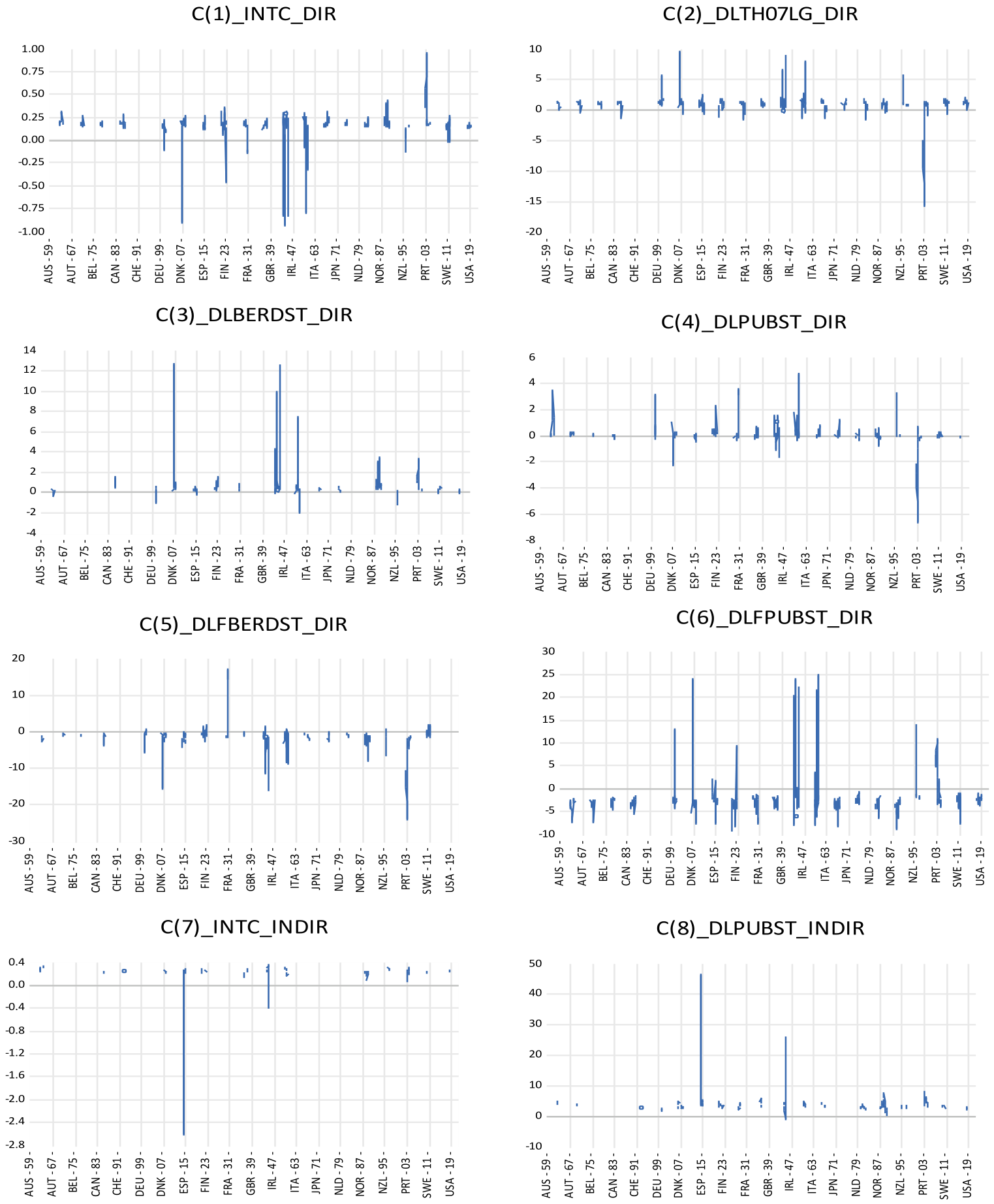
Table 18.
Basic statistics of functional regression coefficients of productivity function and first-order conditions (a).
Figure 3.
The sum of direct and indirect effects of public R&D on technical change.
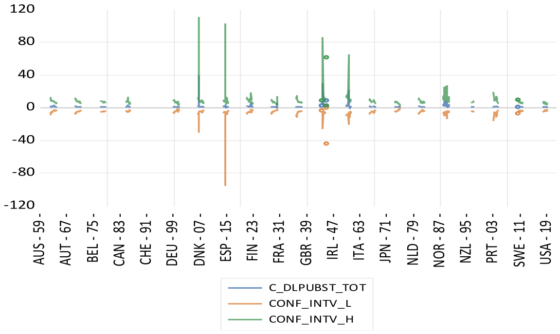
The lagged dependent variable has, on average, a near-unity coefficient of 0.97, whereas the growth rate version of the variable in the data is stationary (see Table 1). Private R&D in (1b) has mainly positive coefficients around 0.43, with a standard deviation that is more than twice as high. Direct public R&D in (1b) has a positive mean and a negative median, and also a relatively large standard deviation.
The coefficients of foreign R&D variables have high standard deviations and high means and medians. Only C(7) and C(8) have higher means and medians than standard deviations. Overall, the method of functional coefficients in our case produces a strong variability in the estimated coefficients. All maximum values are positive, and all minimum values are negative, implying that no variable has only positive coefficients. Figure 2 shows in detail where and how many effects are negative or positive. It is an advantage of the functional coefficient regression method that we can see positive and negative coefficients side by side in different parts of the panel structure. The intercept of the indirect effect, c(7), has very high growth rates compared to what one might expect as BERD-biased technical change or growth of inefficiency (Table 18, row 7, and the lower left graph of Figure 2); the separability of CD, CES, or VES functions may be worth reconsidering.18 The coefficient of public R&D, with a mean of 3.276, a median of 2.965, and a standard deviation of 2.51, would suggest that each percentage point higher growth rate of public R&D turns into 3 percentage points higher growth of private R&D, which is a strong effect of public–private interaction. The wide dispersion of the coefficients is considered in greater detail in the form of kernel density estimates in Appendix C. The high coefficients of the lagged dependent variable raise the issue of unit roots again. In panel data analysis of Table 1, the unit root hypothesis has been rejected. Similarly, in time series studies and panel VECM studies, there are no unit roots for growth rates (Soete et al., 2022; Ziesemer, 2024c). We show in Figure 4 below that the coefficients estimated here are falling in expected value starting from near unit values, and their high levels are not even statistically significant. Moreover, panel unit root tests on the estimated coefficient series have p = 0.0000.19 All these arguments would suggest that there is no unit root problem for a longer time, but lagged dependent variables matter to a decreasing extent.
The insertion of (5) into (1b) yields c(4) + c(3)xc(8) as the total effect of public R&D on technical change, as shown in Figure 3 with , 1996–2019 or shorter, which is a small number of functional coefficients per country. The corresponding standard statistics are shown in the last row of Table 18.
The maximum of 332.9 (IRL 2019) is deleted in Figure 3 to make the other values more clearly visible; Appendix E investigates this observation in detail. The positive indirect effect clearly outweighs the often negative direct effect in Figure 2 and thereby supports the idea of Park (1995) and Sveikauskas (2007), which is supported by the analysis of Soete et al. (2022).
However, the lower confidence interval (c(4) + c(3xc(8) +- 1.96SE) is in the negative area (the only exception is the deleted value).20 A negative lower confidence bound indicates the high risk of doing public R&D in spite of the positive mean and median. The internal rates of return reported in Ziesemer (2024a) indicate that there is an ex post compensation for this risk. In terms of policymakers’ objective functions surveyed by Brock and Durlauf (2001), a sum of positively weighted expected value of the policy effects and a negatively weighted standard error or variance, undertaking additional public R&D investment requires a low weight for the variance or standard deviation, which is a low degree of ambiguity in a special case of Knightian uncertainty.
5.4. Linking the Results to the Productivity Slowdown
Having shown the functional coefficient results in Figure 2 and Figure 3, and A1–A15, the question is now how this relates to the productivity slowdown. From the perspective of functional coefficient regressions, the question is what the trends in the coefficients of Figure 2 are. To see this, we regress each coefficient series on its own one or two lags, a time trend, which is an autoregressive process correcting for serial correlation. In case of doubts about the best specification, we use the covariance proportion of the Theil inequality coefficient, which consists of the bias proportion, the uncertainty proportion, and the covariance proportion as unexplained ‘rest’, which should be high. Table 19 reports these results. For the interpretation, it seems most useful to imagine the standard graph of a difference equation with x(−1) and x on the axes. In all cases, we do have a (sum of) slope coefficient(s) below unity and larger than minus unity, which would ensure stability. However, in five (one) of our nine cases, the time trend shifts the equation line down (up) and along the intersection with the 45-degree line; coefficients then fall (increase). For dlberdst, c(3), and dlfberdst, c(5), there is no such trend, and because of the intercepts, stability leads in the long run to a negative coefficient for foreign and a positive coefficient for domestic private R&D, meaning that foreign competition matters more than foreign spillovers from private R&D. The coefficient of dlfpubst, c(6), has a strongly positive trend and, therefore, will increase unless a structural break stops it. Foreign public R&D, therefore, has strongly positive spillovers in the future when the negative intercept is dominated by the positive trend; public R&D increasingly mutually benefits the 21 countries.
Table 19.
Dynamic trend analysis for functional coefficient estimates (a).
A zero trend is shown for c(7), the intercept of (5); with a positive intercept and slope below unity, it converges to a positive constant value. The interpretation is that inefficiency or BERD-biased technical change has positive and constant growth rates. A negative time trend also applies to the sum of direct and indirect effects of public R&D in the last column of Table 19, and also to its underlying parts c(4) and c(8).
Structural breaks stopping the trends in the future may of course change this, as these trends running into negative coefficients cannot go on for infinite time. Moreover, the cause of the trends does not follow from this analysis; the functional series driving the coefficients may themselves have underlying driving forces that may stem from business or government decisions or market developments.
Figure 4 shows conditional extrapolations of all the univariate trends of the functional coefficients of (1b) under the estimated autoregressive specification (rather than forecasts of economically expected future elasticities) together with their two standard error bounds. The purpose here is only to make the expected trend in the coefficients visible. It is not to give an explanation again, and, therefore, the functional coefficient series are not included again. The two standard error bounds of the prediction intervals are mostly on different sides of the axes and indicate high uncertainty of conditional extrapolations.
Figure 4.
Autoregressive conditional extrapolations of functional regression coefficients of the productivity function. Functional regression coefficients C(1) to C(6) from the productivity function; trend and confidence interval per country across years. Conditional extrapolations of expected values of functional coefficients have high uncertainty and trends, with two exceptions, domestic and foreign private R&D.
As suggested by the interpretation of the regressions of Table 19, only domestic and foreign private R&D variables go towards having constant coefficients. Foreign public R&D has increasing coefficients. All other variables have decreasing coefficients; a decreasing intercept suggests falling exogenous technical progress in the productivity growth function (1b).
Figure 5 shows that the conditional extrapolations of intercept and slope of (5) under the estimated autoregressive specification go to a constant expected value and thereby indicate a constant BERD-biased technical change or/and increasing inefficiency; as parts of the confidence interval are negative, there is some uncertainty about the positive value of this result. Whereas the slope coefficient goes down, the lower confidence bound is mostly negative, indicating again that the positive level of the line has some uncertainty. The total effect of public R&D goes down, which is in line with the discussion of the last column of Table 19. The two standard error bounds of the prediction intervals are often on different sides of the axes and indicate high uncertainty for the positive level of conditional extrapolations. The low statistical significance may come from the lack of adding explanatory variables again and from limited panel length. For Figure A1, Figure A2, Figure A3, Figure A4, Figure A5, Figure A6, Figure A7, Figure A8, Figure A9, Figure A10, Figure A11, Figure A12, Figure A13, Figure A14 and Figure A15, the number of observations is stated as 504 to 1155. For c(3) × c(8), it is 405, leading to an average of T = 19.
Figure 5.
Autoregressive conditional extrapolations of functional regression coefficients of the first-order conditions and the total effect of public R&D. Functional regression coefficients C(7) and C(8) in the private–public R&D relation and total effect of public R&D growth on productivity growth, and C(3) × C(8) + C(4) show high uncertainty and trends per country across years.
In Table 19, some numbers of observations are even shorter. As this hinders the long-run covariance formula from converging, we had to give up taking into account the heteroscedasticity and autocorrelation consistency in the estimation of the confidence interval for Figure 3 in Appendix D, which implies additional uncertainty on the confidence interval.
6. Summary and Conclusions
Our direct estimates demonstrate that regression coefficients for R&D variables in countries’ productivity functions are mostly not constant and depend on functional coefficient series (smoothing variables), such as lagged growth of human capital, GDP per worker, share of services, and defense R&D, as well as lagged regressors. These coefficient changes may also happen to go on in the future. Therefore, policy conclusions can never be drawn directly from estimates based on past data, and they require much intuition, perhaps based on average values of expected, estimated coefficients, and the assumption of no structural breaks in the average values.
We suggest the following from putting all these partial effects on regression coefficients together to coefficient trends. Panel average values of coefficients for domestic and foreign private R&D, dlberdst and dlfberdst, go to constant values as time passes. Coefficients of foreign public R&D growth go up. Direct, indirect, and total coefficients of public R&D go down. This combines mostly negative direct effects and mostly positive indirect effects, making it hard to predict the overall change in combination with the levels reached. The result here is that coefficients of the total effect of public R&D are positive but are going down with increasing uncertainty. These developments may contribute to the explanation of the productivity slowdown.
Without rigorously establishing this, we cautiously interpret this as a policy aspect that may have contributed to the productivity slowdown, and as a matter of a partial argument, it is plausible that investment in R&D has shifted from public to private R&D in recent decades. This does not necessarily justify the extent to which this has taken place. In the raw data of our panel, public R&D flows as a share of GDP are mostly increasing in the previous century but falling for four (seven) countries in the current century (starting in 2008) see OECD MSTI); the overall growth rate of the GERD/GDP ratio is 1.7 percent and 1.1 percent in the current millennium, falling below one percent when starting in 2008. The fall in the growth rates of public R&D flows, therefore, is stronger than that in GDP, which is caused by the productivity slowdown and some recent crises (Fernald et al., 2025). Falling regression coefficients add to this. On the other hand, if policy can turn public R&D stock growth into positive values, this may increase the coefficients of domestic private and public R&D and perhaps decrease those of foreign R&D if conditional associations are also causal or at least unchanged.
The method of functional coefficient regression allows us to find the coefficients for the whole panel with values differing for each country-year pair. With changing coefficients, it is much harder to calculate the advantages of R&D investments, which is also an innovative insight of this paper with relevance for the administration of innovation policy. This extends the microeconomic uncertainty dimension of innovation (see Dosi, 1988; Cantner & Guerzoni, 2009) to the elasticities of productivity on the macroeconomic level.
In regard to hoping to overcome the productivity slowdown, we can hope for a structural break ahead, phasing out the negative trends in the coefficients. This could perhaps be that the share of services becomes constant; this would stop reducing the effect of public on private R&D. Moreover, technical change could get directed towards services or/and its inputs, as suggested by the logic of induced sectoral technical change in Boppart and Weiss (2013) and Comin et al. (2025). According to Boppart (2014), this redirection of technical change has not yet happened because the prices of industry relative to those of service are still falling in his data. If it happens in the future, it could take a lot of time, though, as in the data of Boppart and Weiss (2013) for durable and non-durable goods, where the delay is thirty years. Similarly, Comin et al. (2025) point out that technical change in services accelerated in the 1980s ‘and achieved the fastest growth rate in the last decade’. However, this is still not enough to get rid of the productivity slowdown. They expect the recovery of TFP growth through innovation in services in 2100. Their model has only private R&D, though.
The reduced incentive through falling coefficients does not exclude the possibility of going against this with policies of higher expenditure on human capital and public R&D. In addition to waiting for market-driven sectoral effects, education policy could enlarge human capital growth in order to improve the effect of public R&D on private R&D that we have shown to depend on human capital according to Table 17. Soete et al. (2022) have shown that strengthening the domestic link between public and private R&D leads to stronger effects of public R&D growth on TFP growth. A stronger positive effect on the lagged dependent variable can also be achieved through more human capital growth. This may require targeting education to areas able to link technical change and R&D. Improved education could go together with mission-oriented and public R&D, which both increase TFP and GDP growth (Ziesemer, 2021a, 2024b; Soete et al., 2022). Here, we have added to this that higher public R&D growth enhances the regression coefficients of private and public R&D and reduces those of foreign R&D.
We do not claim to have established causal effects of R&D policy, education policy, or structural change but rather that these ideas are going beyond the work done in this paper. An outlook from here to future research suggests researching these and the following issues. Regarding modeling, specifying nested CES functions may lead to richer first-order equations than just linking domestic private and public R&D, but they would also be highly nonlinear. Other functional coefficient series may be found by authors with a different background knowledge; this may lead to more or less different shifts in the coefficients. Current progress in econometrics in the area of functional coefficient regressions is going through all sub-areas of econometrics that dynamic panel data analysis has gone through (fixed effects, endogeneity, instrument choice, cross-section dependence, common factors, unit root and cointegration analysis for regressors and functional series); it will take some time until these issues are not only treated separately, and scientific teams of package providers have made decisions on which of the new elements can be put together meaningfully. Therefore, these issues are also limitations of our paper.
Funding
This research received no external funding.
Data Availability Statement
The data are from Ziesemer (2026). The data are available at the MERIT Dataverse: https://doi.org/10.34894/TW6W8N.
Acknowledgments
I am grateful to four anonymous reviewers, Mercedes Menéndez De Medina, and Bart Verspagen, for their useful comments. Responsibility is entirely mine. The author has reviewed and edited the output and takes full responsibility for the content of this publication.
Conflicts of Interest
The author declares no conflicts of interest.
Appendix A. Histograms of Functional Variable Series
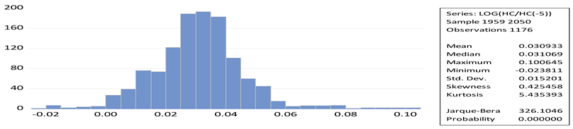
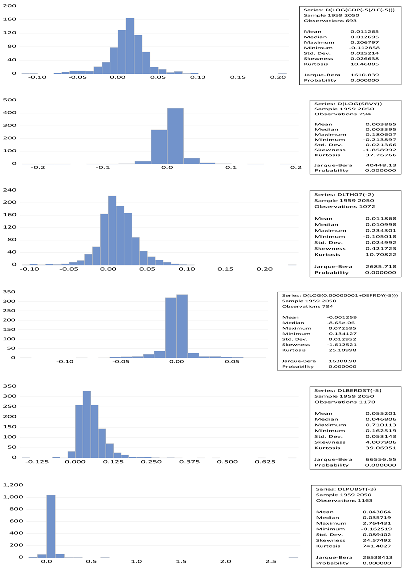
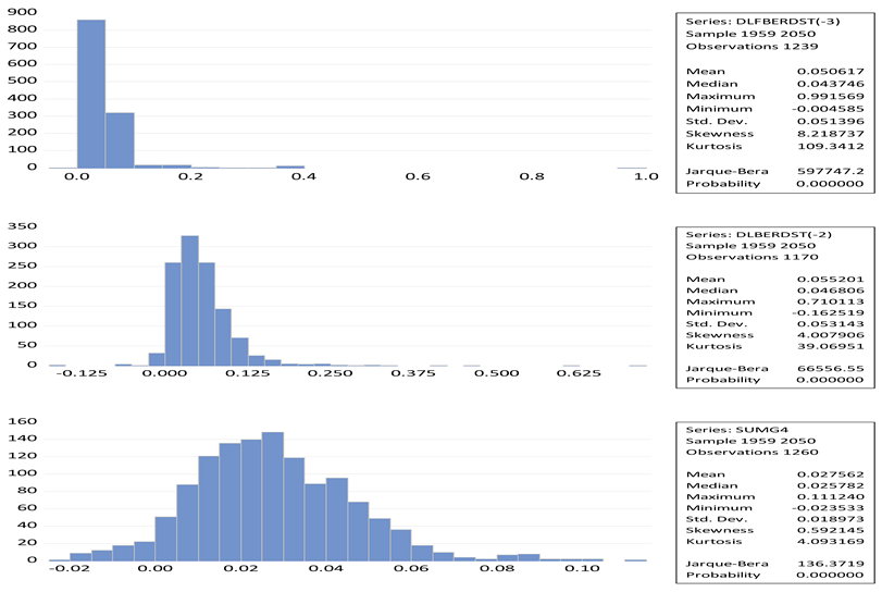
Appendix B. Figures of Partial Contributions of Functional Coefficient Series with Regressors on the Vertical and Functional Series on the Horizontal Axis
Figure A1.
The partial contributions of five-year human capital growth to the regression coefficients of the productivity function. Notes: Dependent variable: DLTH07. Method: Functional coefficients. Sample (adjusted): 1976–2019. Included observations: 1023 after adjustments. Functional coefficient series: LOG(hc/hc(−5)). Kernel: Epanechnikov. Local polynomial degree: 4. Bandwidth: 0.1 (automatic: CV). Localization grid: Functional coefficient series.
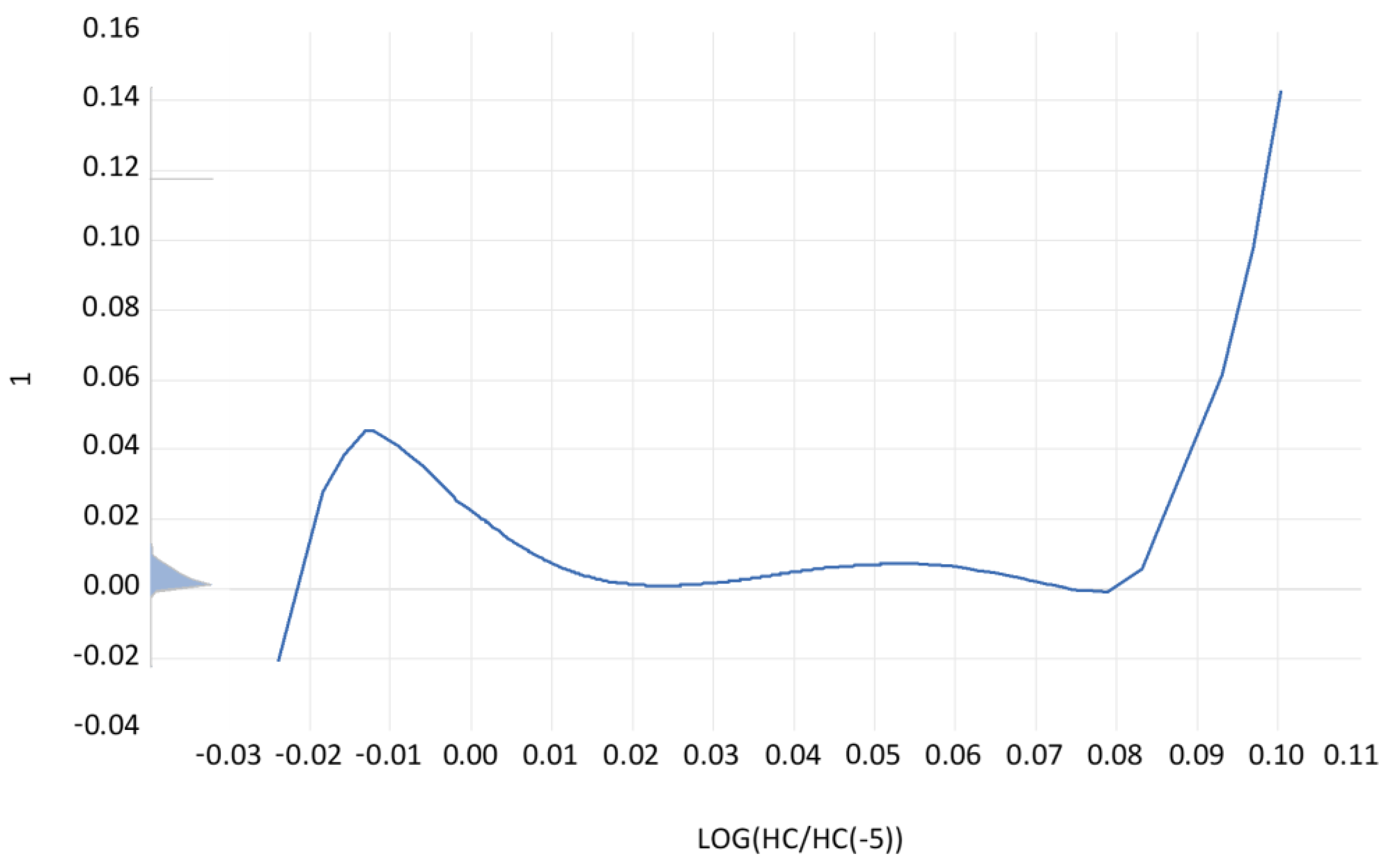
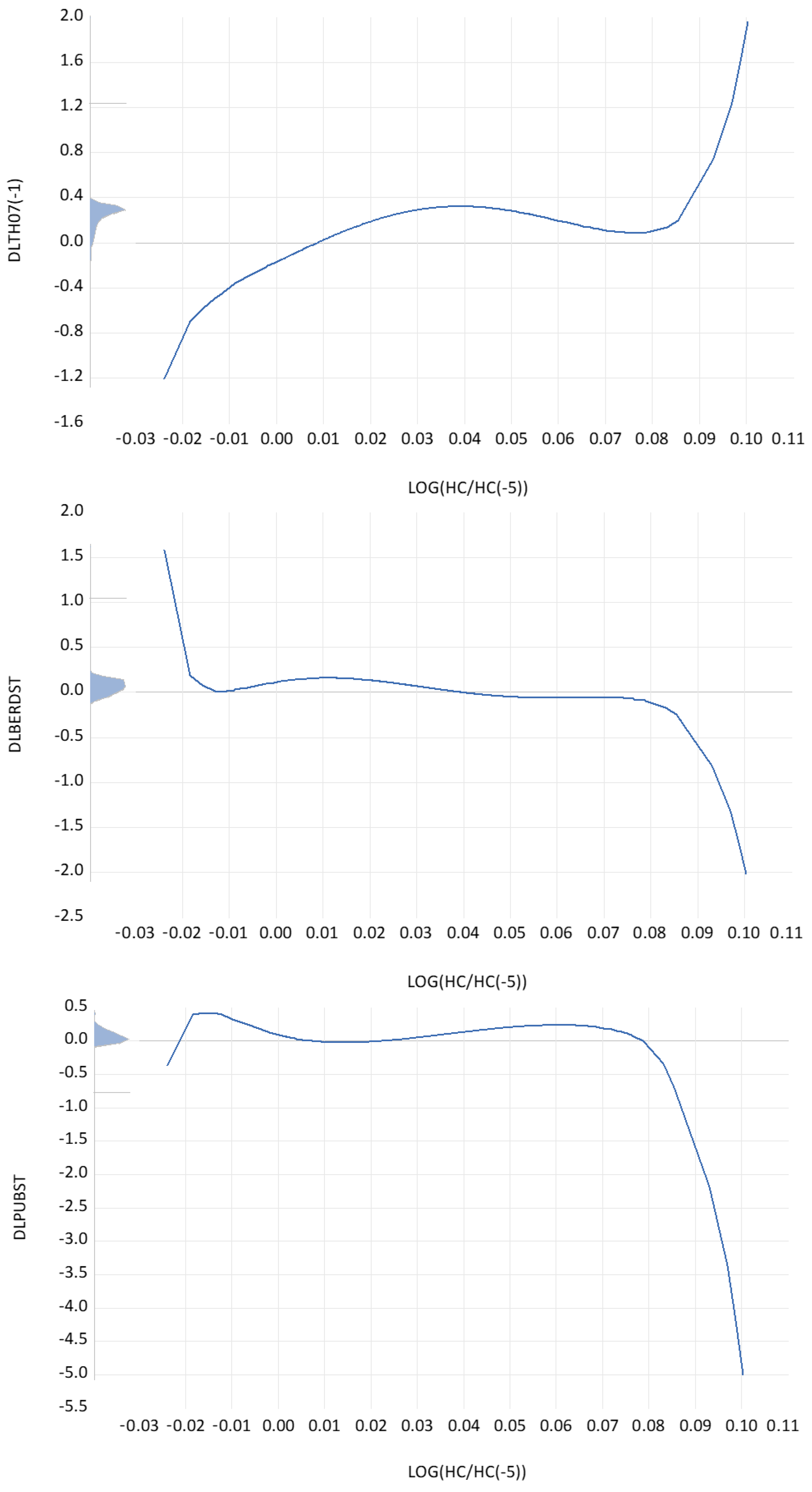
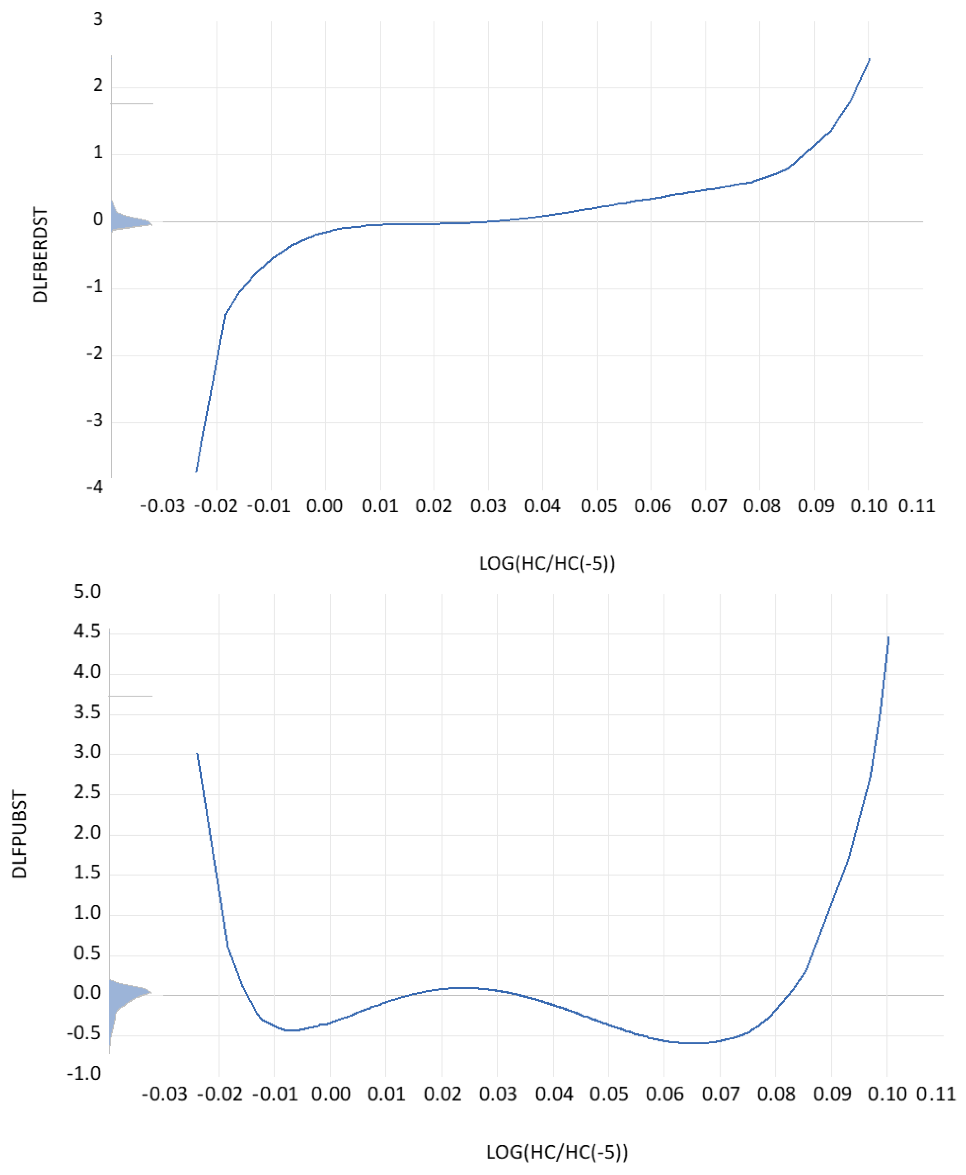
Figure A2.
The partial contributions of past growth rates of GDP per worker to the regression coefficients of the productivity function. Notes: Dependent variable: DLTH07. Method: Functional coefficients. Sample (adjusted): 1996–2019. Included observations: 504 after adjustments. Functional coefficient series: D(LOG(GDP(−5)/(LF(−5)))). Kernel: Epanechnikov. Local polynomial degree: 3. Bandwidth: 0.1000 (automatic: CV). Localization grid: Functional coefficient series.
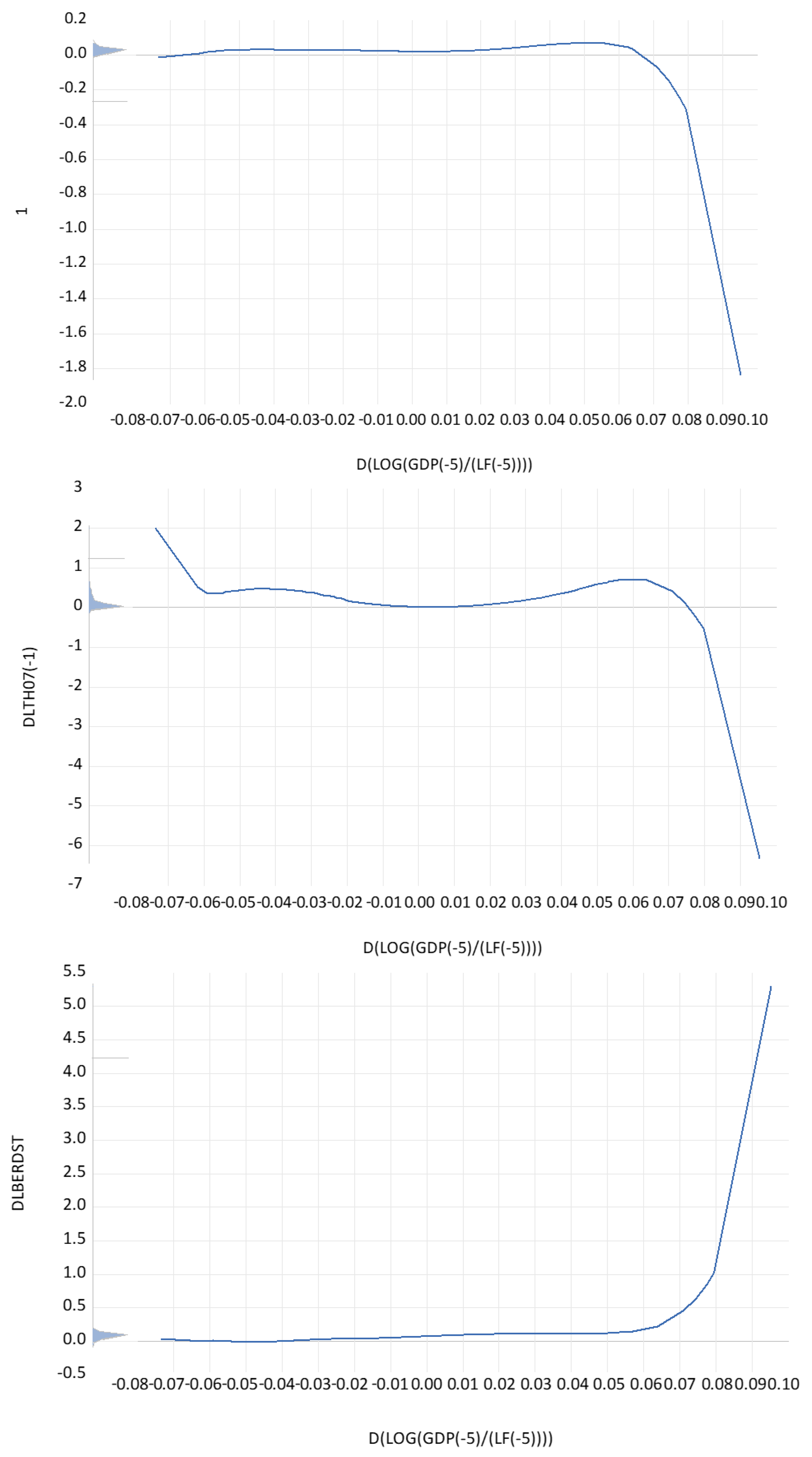
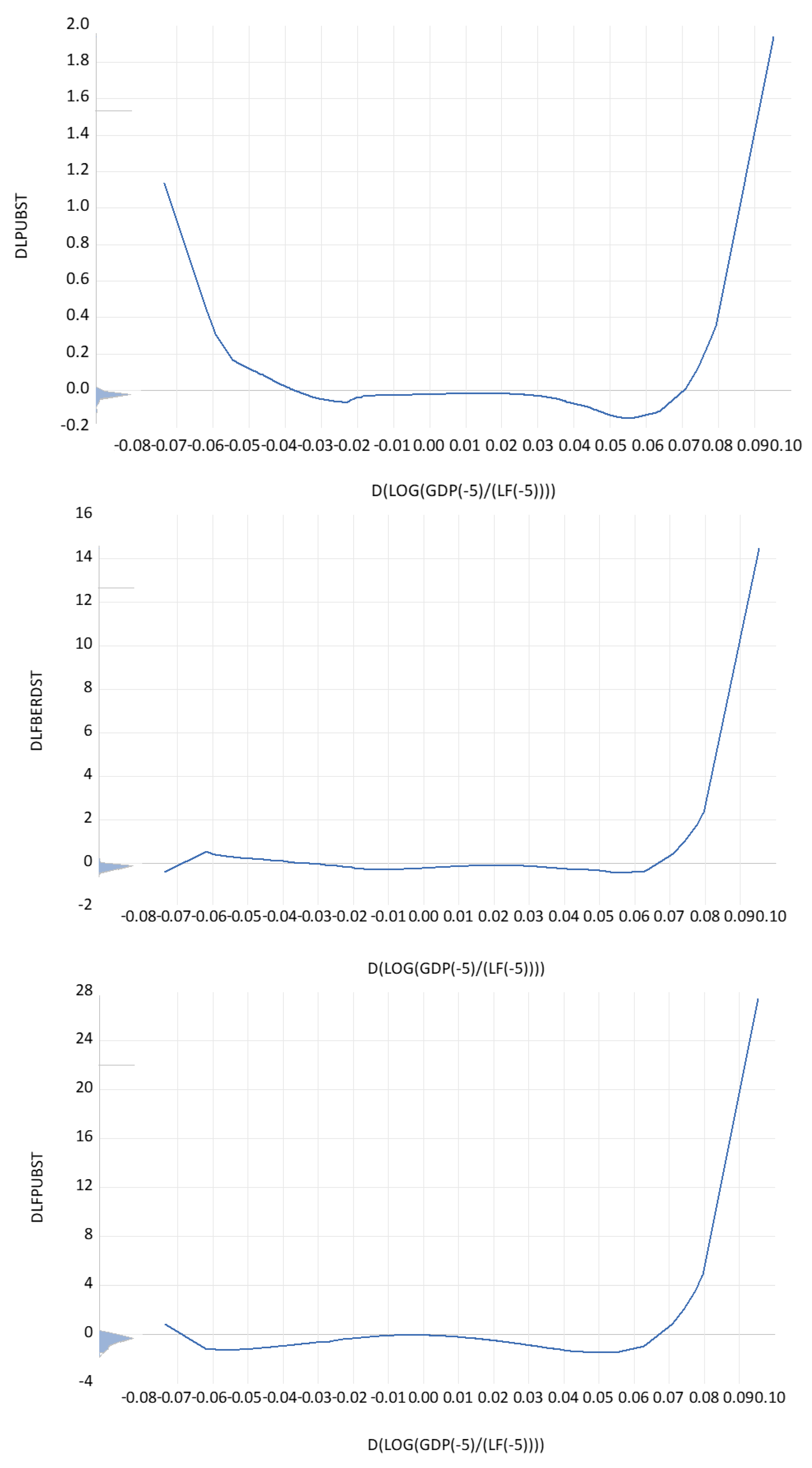
Figure A3.
The partial contributions of services (% GDP) growth to the regression coefficients of the productivity function. Notes. Dependent variable: DLTH07. Method: Functional coefficients. Sample (adjusted): 1991–2019. Included observations: 700 after adjustments. Functional coefficient series: D(LOG(SRVY)). Kernel: Epanechnikov. Local polynomial degree: 2. Bandwidth: 0.2594 (automatic: CV). Localization grid: Functional coefficient series.
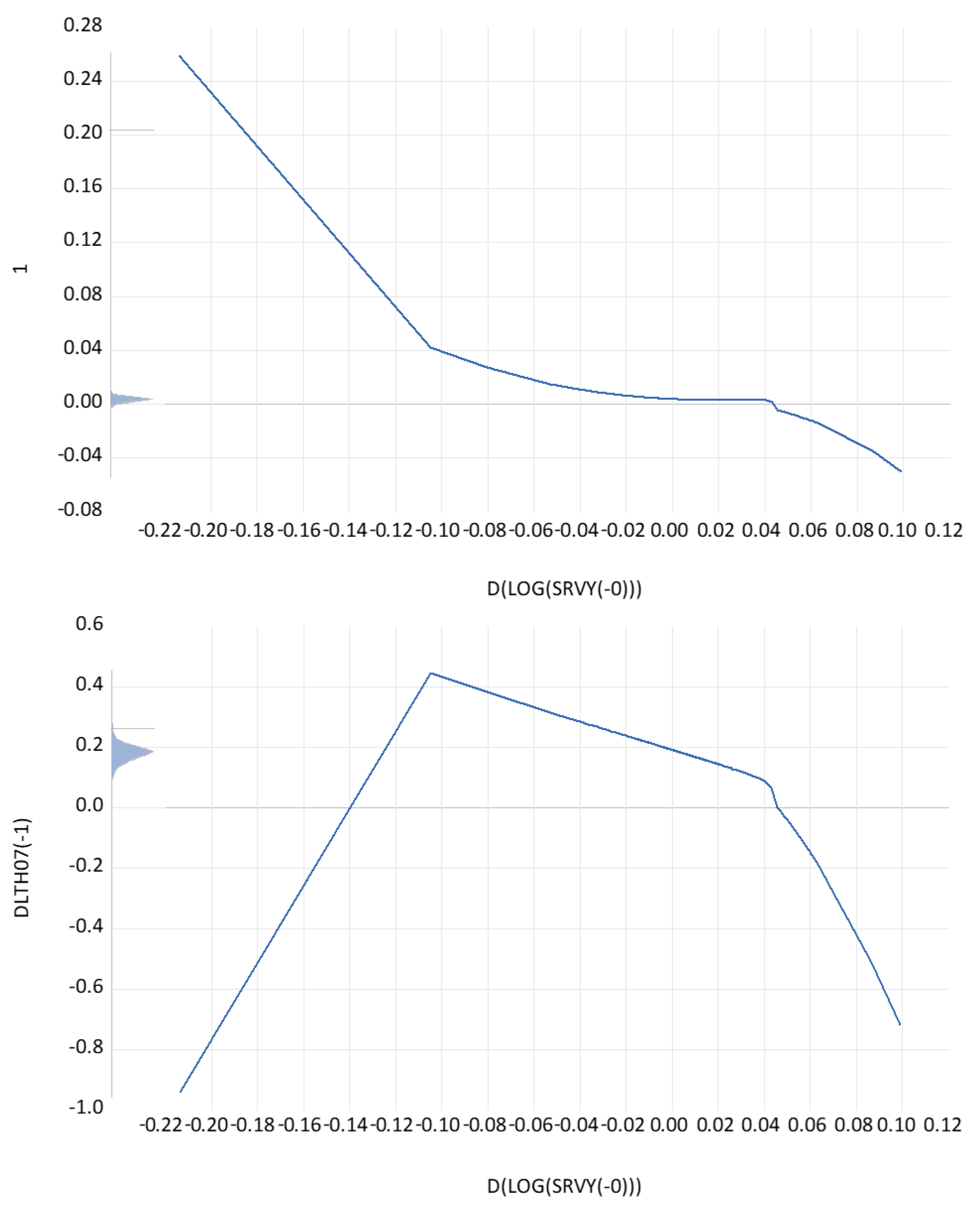
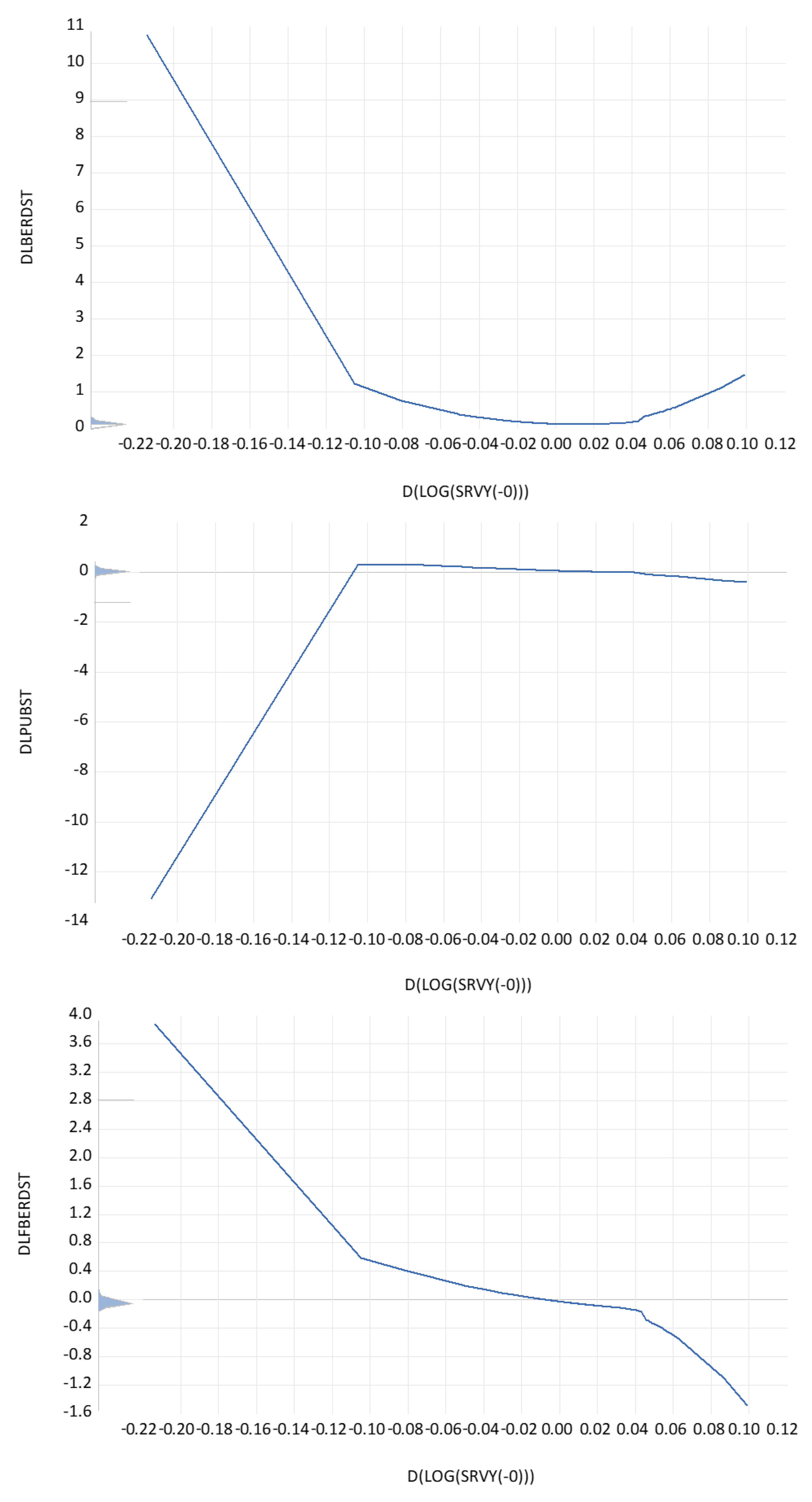
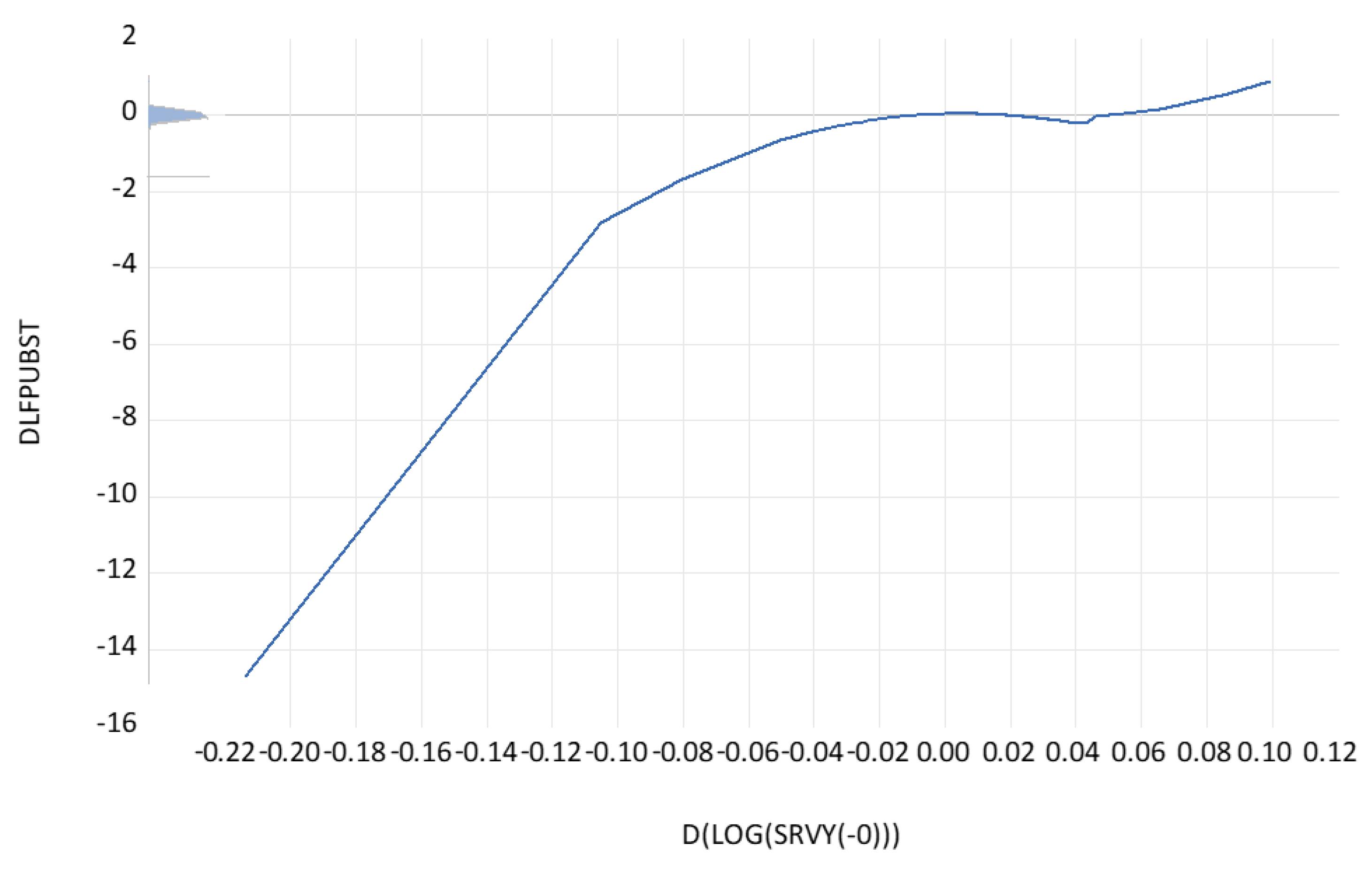
Figure A4.
The partial contributions of defense R&D (% GDP) growth to the regression coefficients of the productivity function. Notes. Dependent variable: DLTH07. Method: Functional coefficients. Sample (adjusted): 1987–2019. Included observations: 616 after adjustments. Functional coefficient series: D(LOG(0.00000001 + DEFRDY(−5))). Kernel: Epanechnikov. Local polynomial degree: 3. Bandwidth: 1.0835 (automatic: CV). Localization grid: Functional coefficient series.
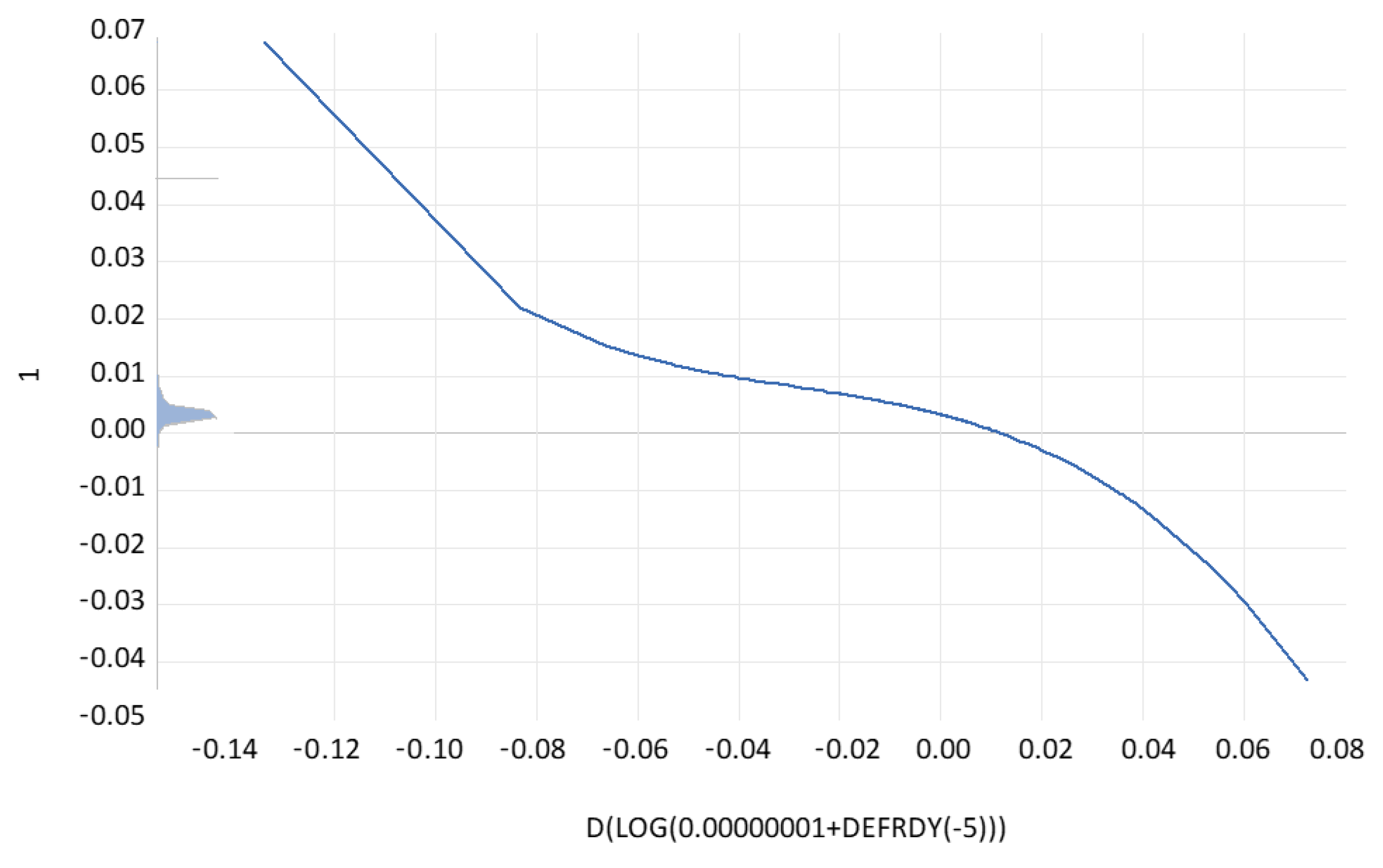
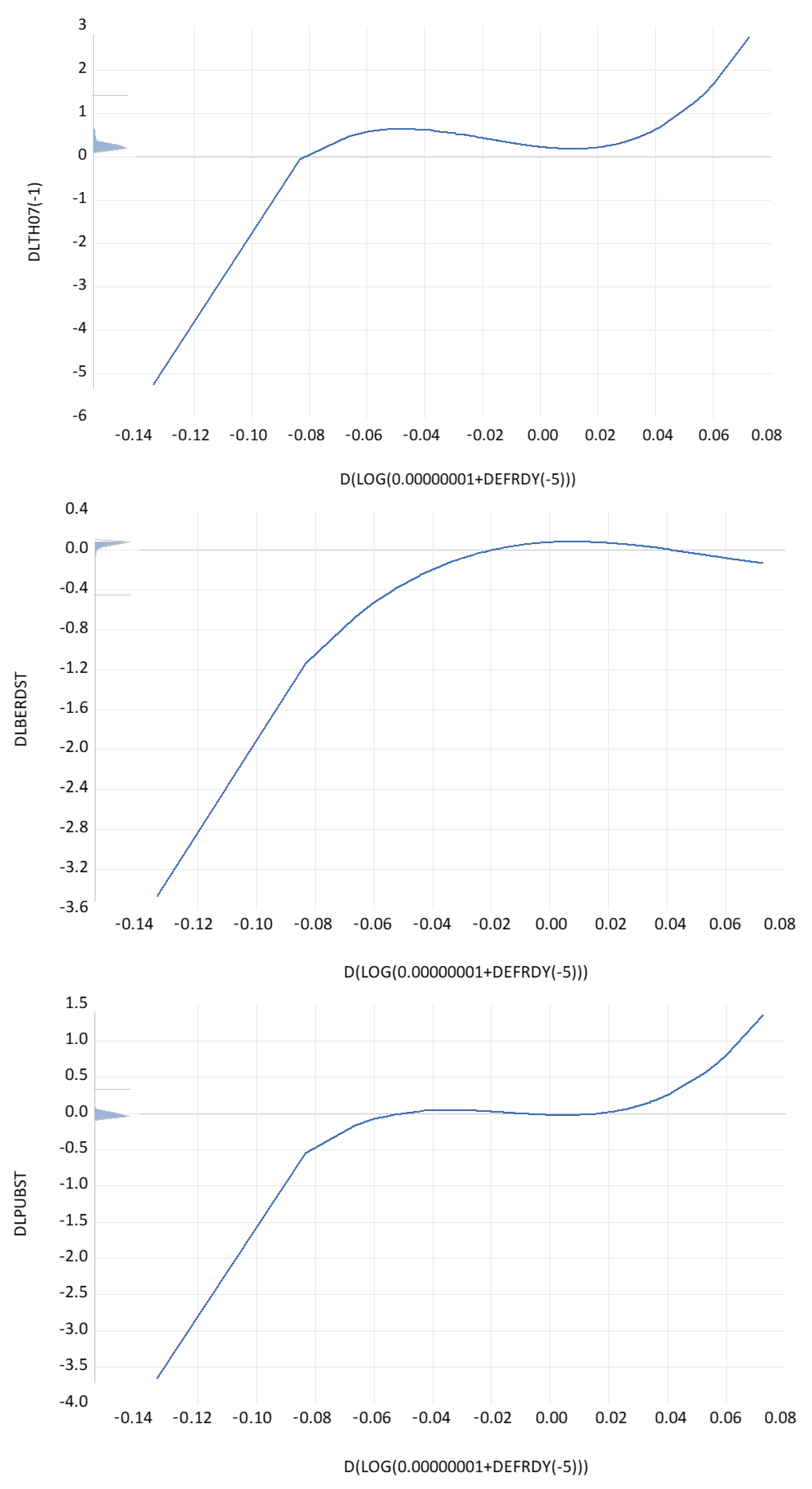
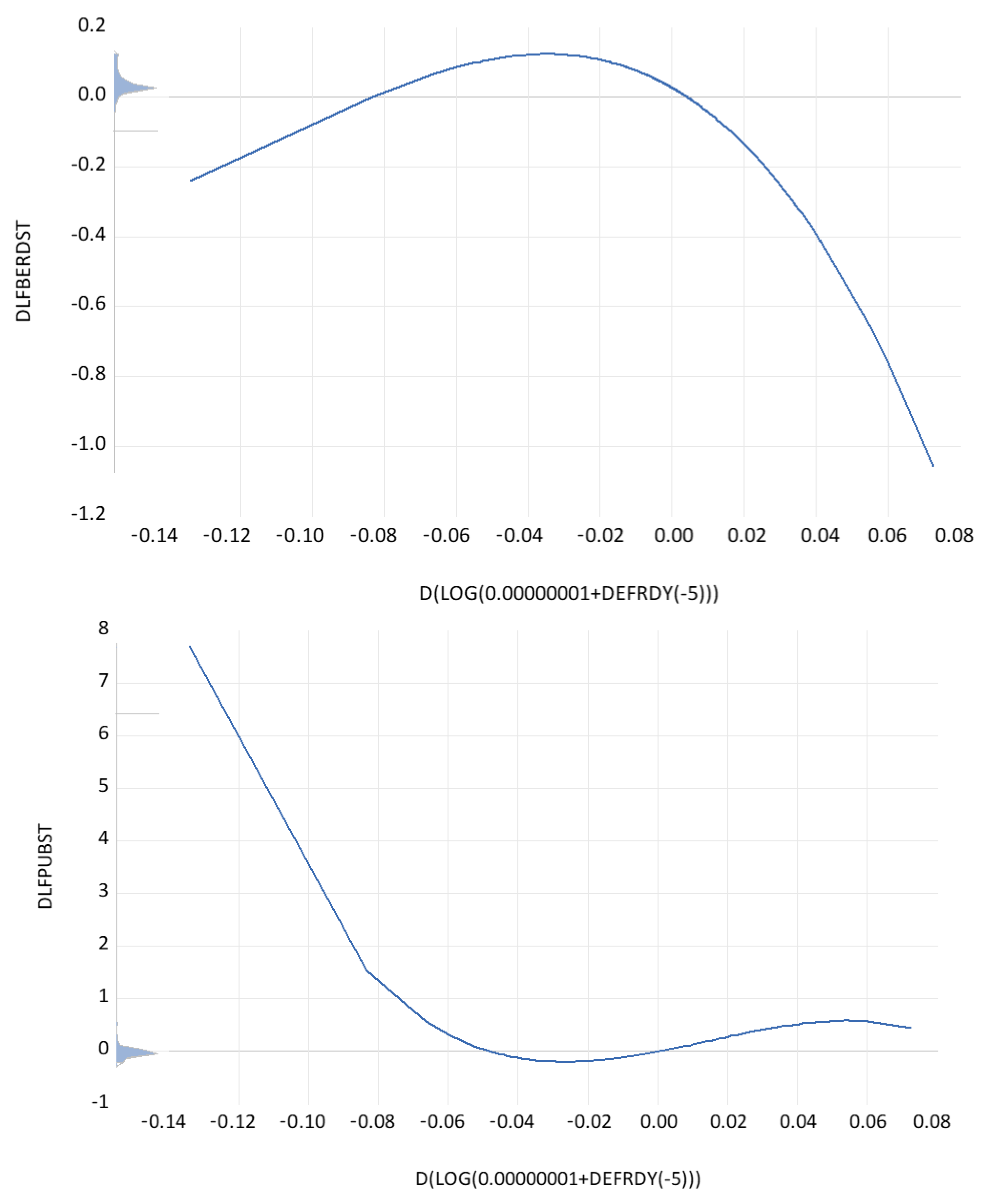
Figure A5.
The partial contributions of twice-lagged labor productivity growth to the regression coefficients of the productivity function. Notes. Dependent variable: DLTH07. Method: Functional coefficients. Sample (adjusted): 1976–2019. Included observations: 1005 after adjustments. Functional coefficient series: DLTH07(−2). Kernel: Epanechnikov. Local polynomial degree: 3. Bandwidth: 0.2853 (automatic: CV). Localization grid: Functional coefficient series.
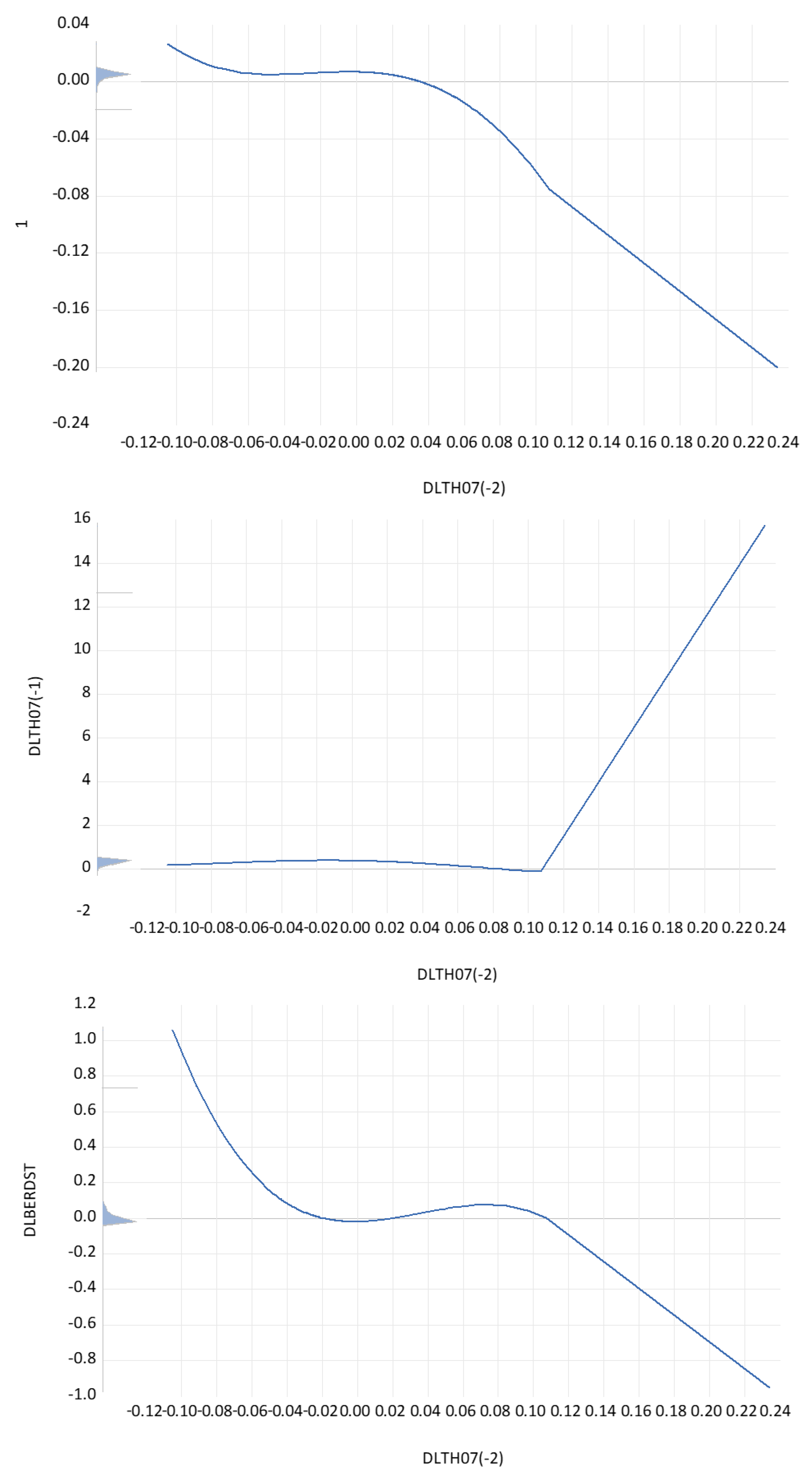
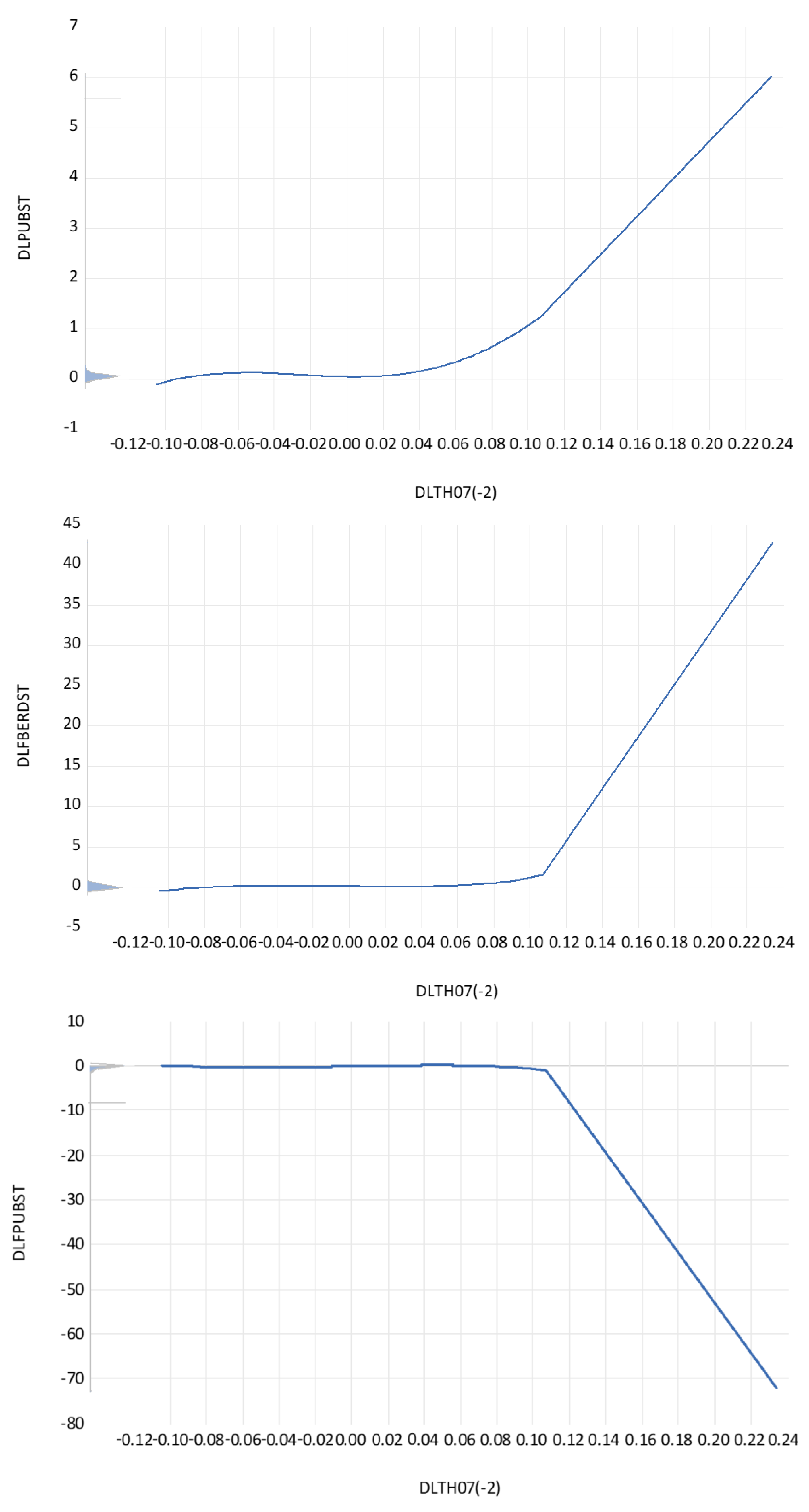
Figure A6.
The partial contributions of dlberdst(−5) to the regression coefficients of the productivity function. Notes. Dependent variable: DLTH07. Method: Functional coefficients. Sample (adjusted): 1981–2019. Included observations: 992 after adjustments. Functional coefficient series: DLBERDST(−5). Kernel: Epanechnikov. Local polynomial degree: 1 (degree 2 is not smooth; degree 3 does not give constant coefficient tests). Bandwidth: 0.4595 (automatic: CV). Localization grid: Functional coefficient series.
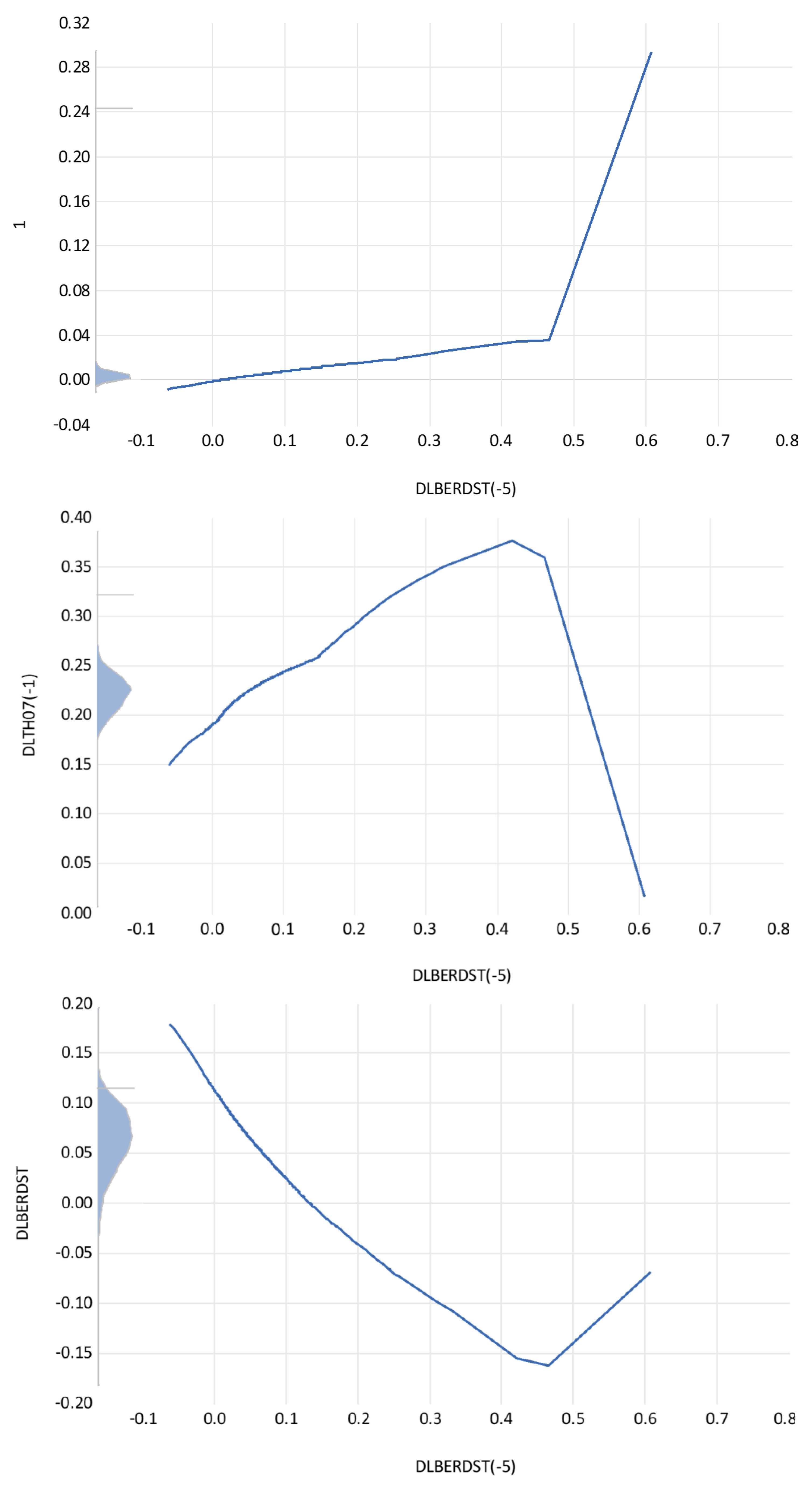
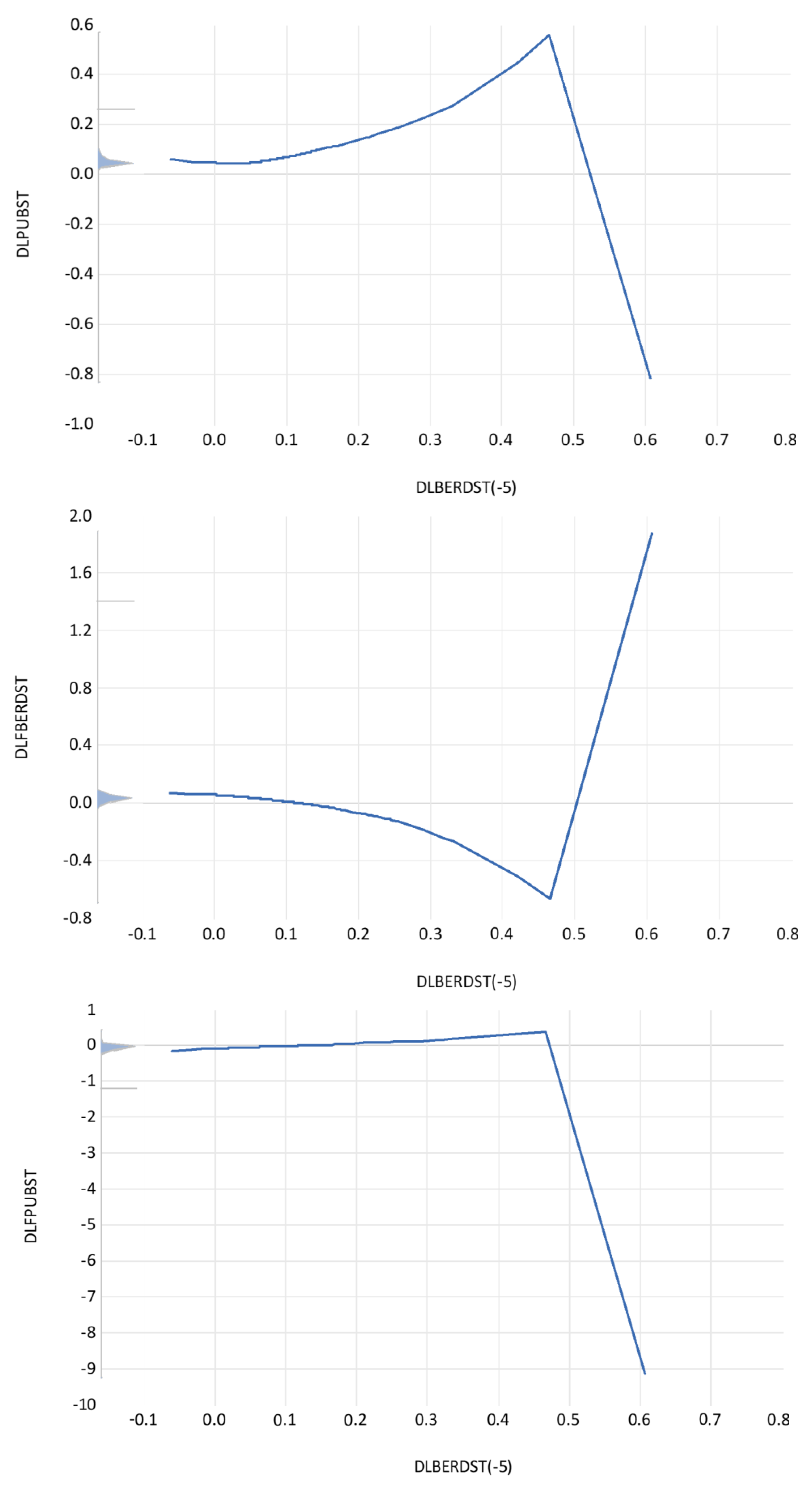
Figure A7.
The partial contributions of public R&D stock growth, dlpubst(−3), to the regression coefficients of the productivity function. Notes. Dependent variable: DLTH07. Method: Functional coefficients. Sample (adjusted): 1979–2019. Included observations: 1002 after adjustments. Functional coefficient series: DLPUBST(−3). Kernel: Epanechnikov. Local polynomial degree: 2. Bandwidth: 0.2358 (automatic: CV). Localization grid: Functional coefficient series.
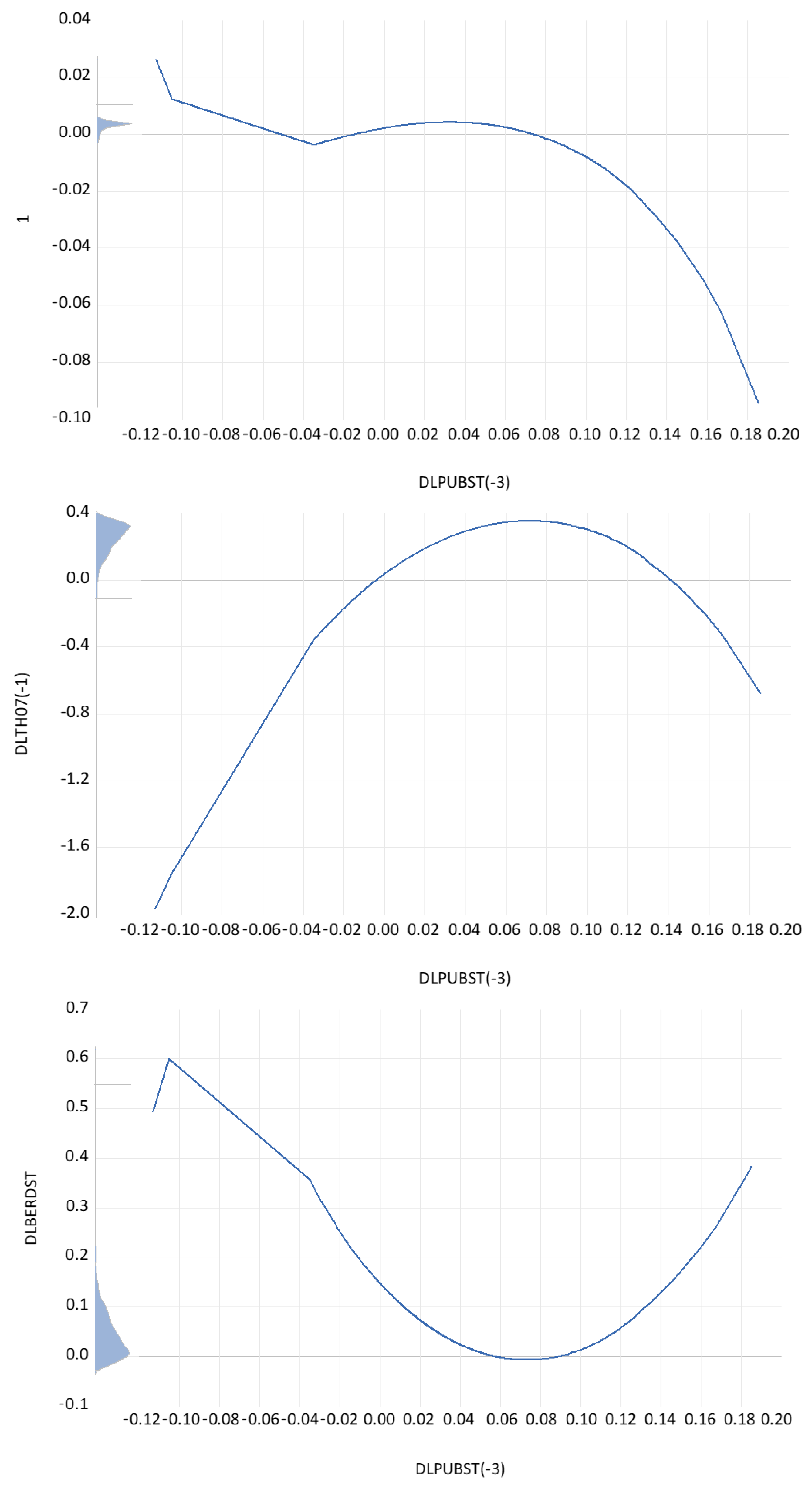
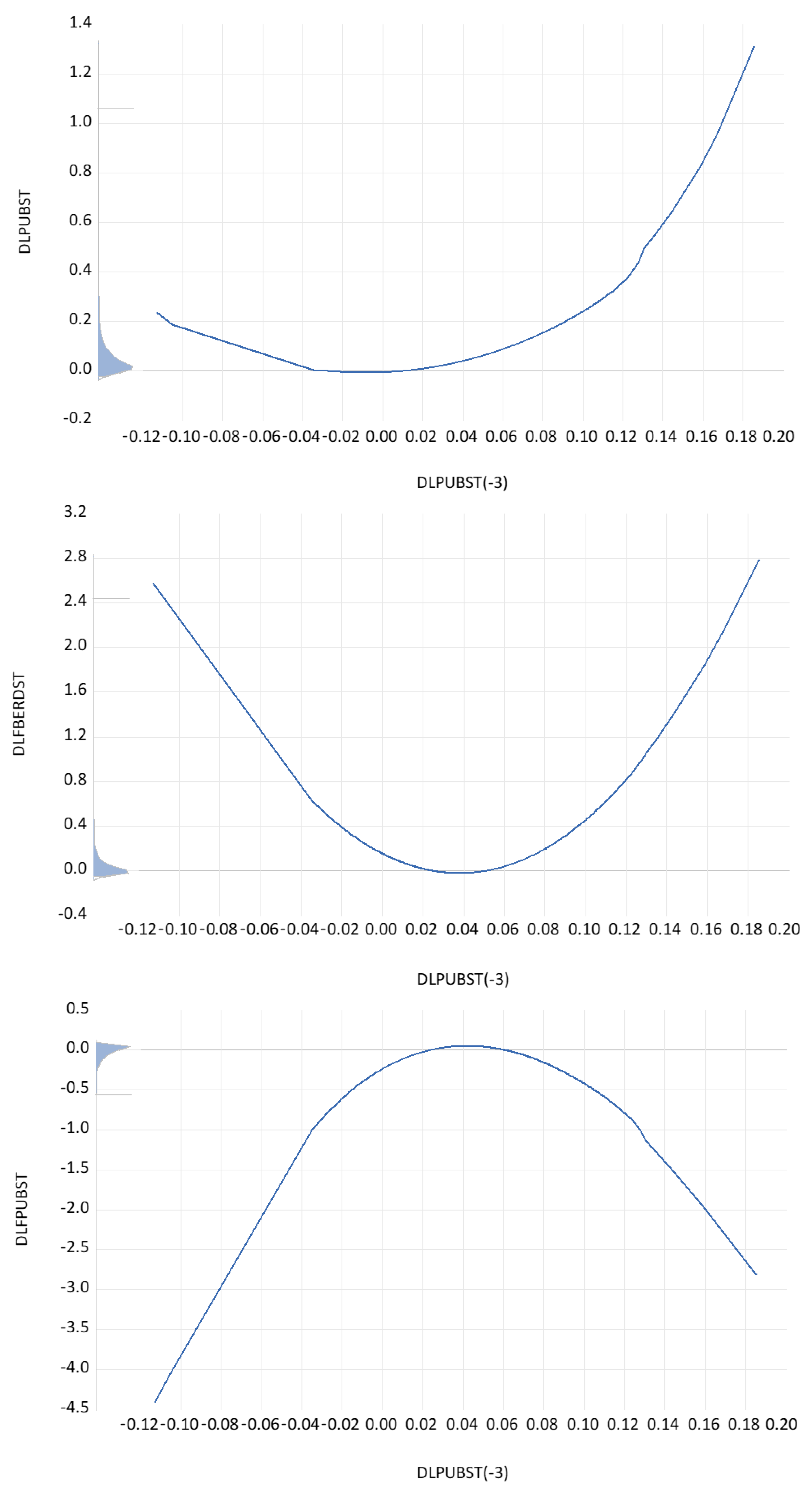
Figure A8.
The partial contributions of the 5-year growth rate of human capital to the regression coefficients of private R&D depending on public R&D. Notes: Dependent variable: DLBERDST. Method: Functional coefficients. Sample (adjusted): 1976–2019. Included observations: 1115 after adjustments. Functional coefficient series: LOG(HC/HC(−5)). Kernel: Epanechnikov. Local polynomial degree: 3. Bandwidth: 0.1000 (automatic: CV). Localization grid: Functional coefficient series.
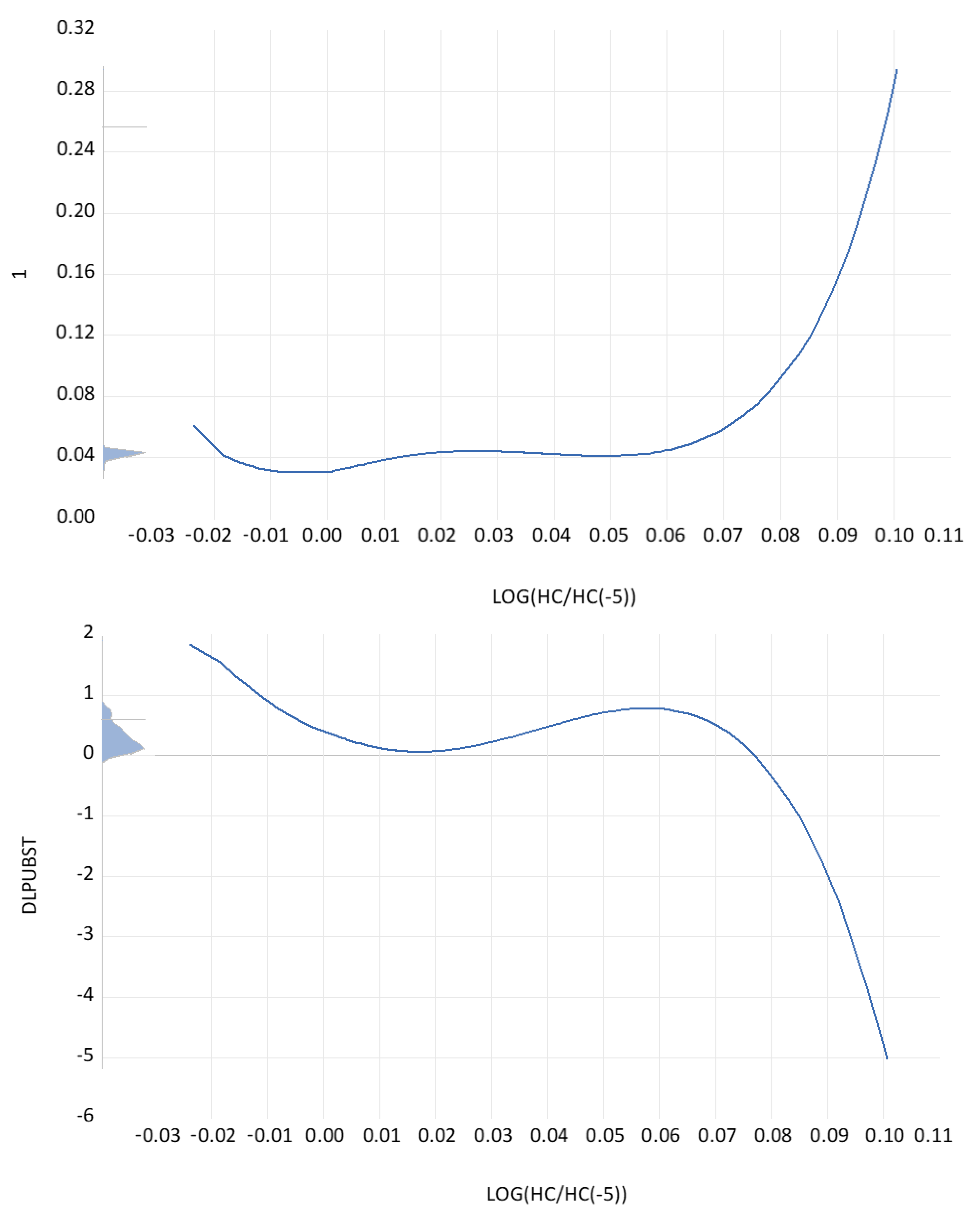
Figure A9.
The partial contribution of growth of services(−3) (%GDP(−3)) to the regression coefficients of private R&D depending on public R&D. Notes. Dependent variable: DLBERDST. Method: Functional coefficients. Sample (adjusted): 1994–2021. Included observations: 695 after adjustments. Functional coefficient series: D(LOG(SRVY(−3))). Kernel: Epanechnikov. Local polynomial degree: 2. Bandwidth: 0.1100 (automatic: CV). Localization grid: Functional coefficient series.
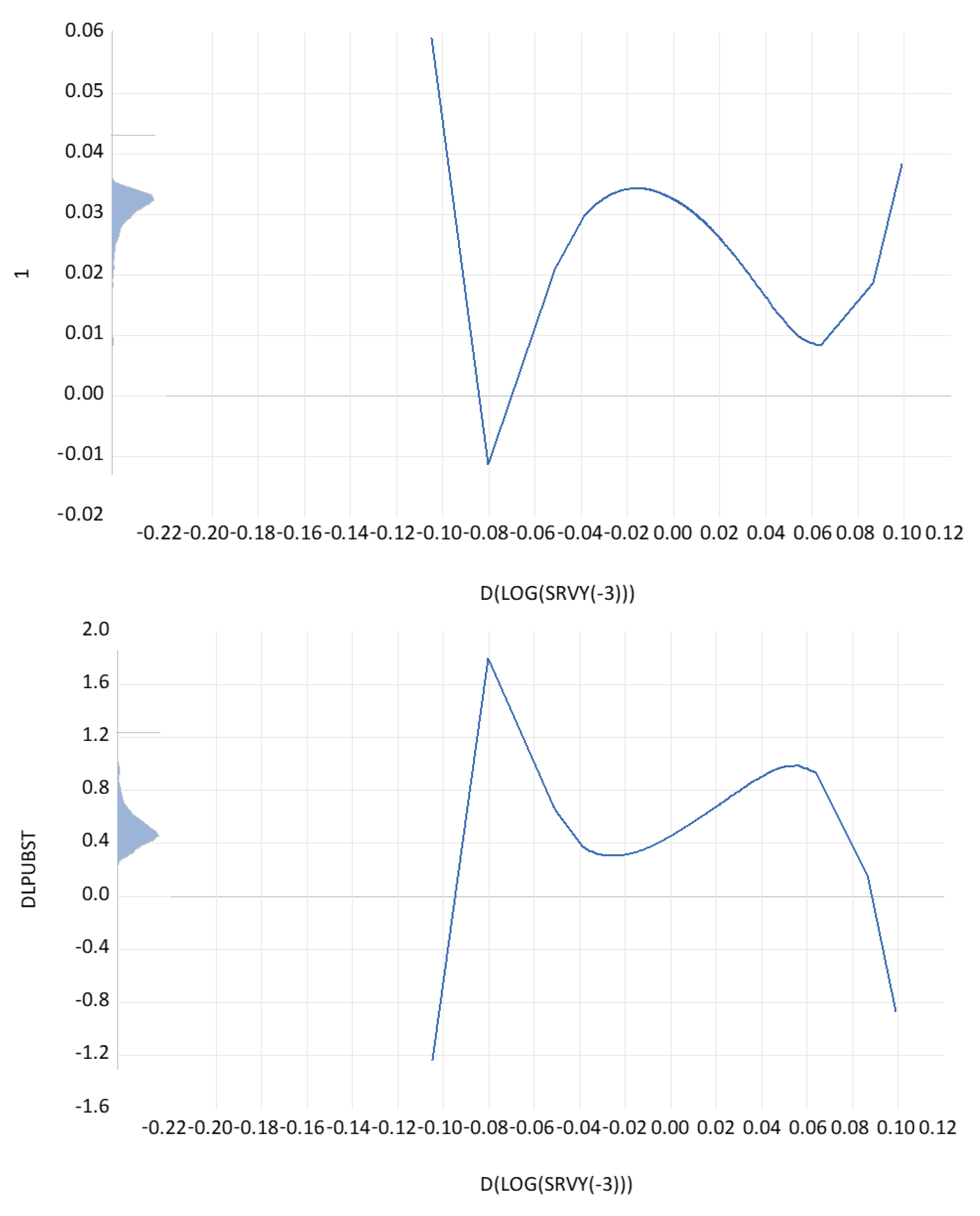
Figure A10.
The partial contribution of services(−4) (%GDP(−4) growth to the regression coefficients of private R&D depending on public R&D. Notes. Dependent variable: DLBERDST. Method: Functional coefficients. Sample (adjusted): 1995–2021. Included observations: 674 after adjustments. Functional coefficient series: D(LOG(SRVY(−4))). Kernel: Epanechnikov. Local polynomial degree: 2. Bandwidth: 0.1000 (automatic: CV). Localization grid: Functional coefficient series.
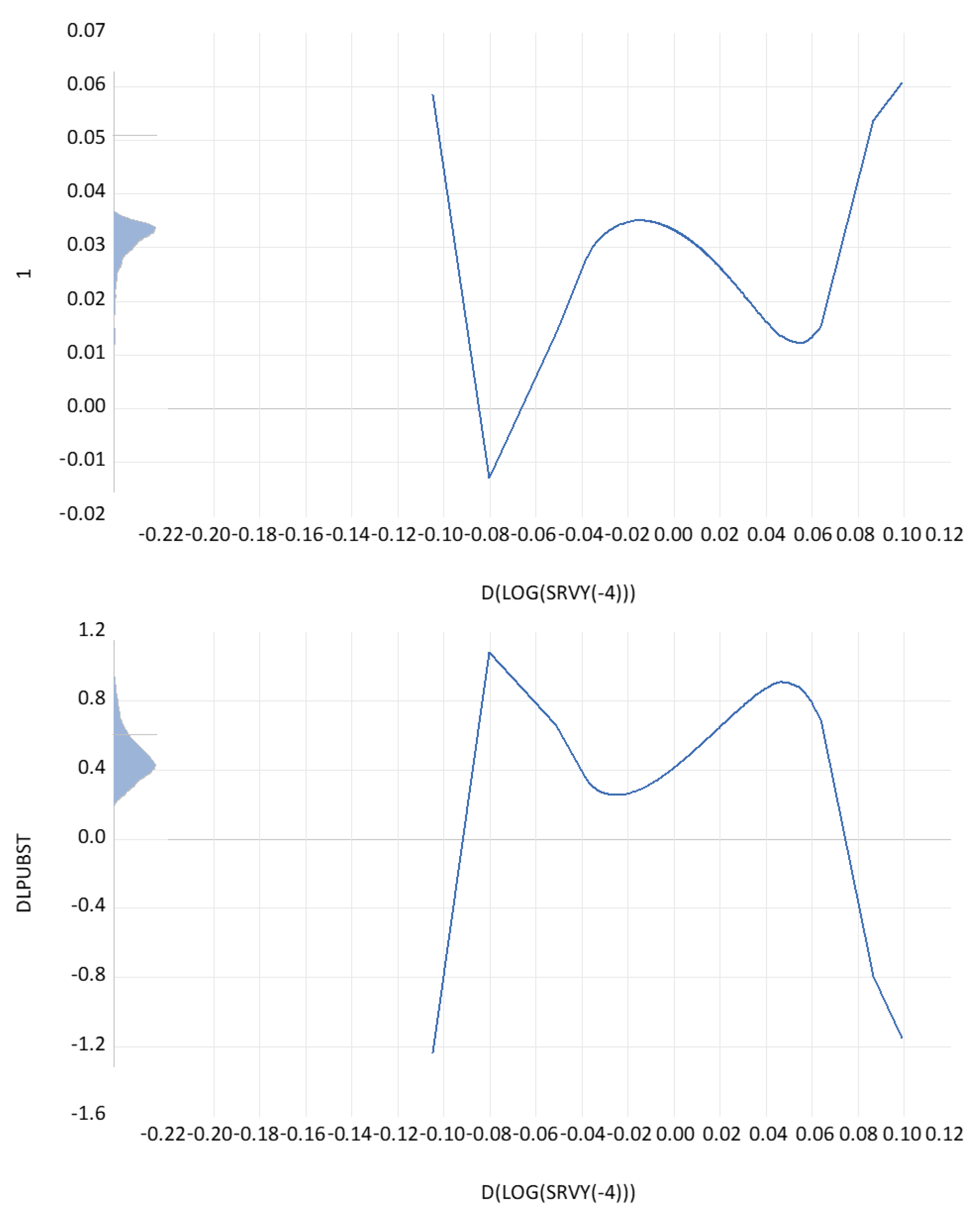
Figure A11.
The partial contribution of service (−5) (%GDP(−5)) growth to the regression coefficients of private R&D depending on public R&D. Notes. Dependent variable: DLBERDST. Method: Functional coefficients. Sample (adjusted): 1996–2021. Included observations: 653 after adjustments. Functional coefficient series: D(LOG(SRVY(−5))). Kernel: Epanechnikov. Local polynomial degree: 3. Bandwidth: 0.1949 (automatic: CV). Localization grid: Functional coefficient series.
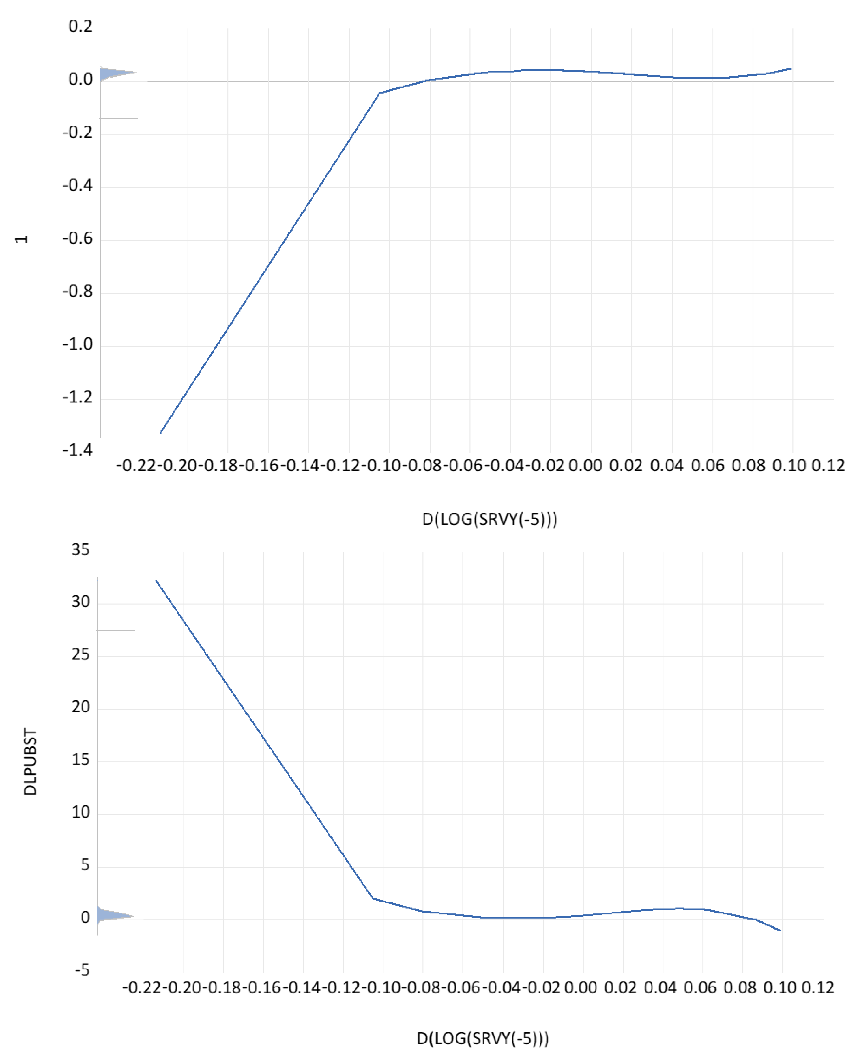
Figure A12.
The partial contribution of defense R&D (%GDP) growth to the regression coefficients of private R&D depending on public R&D. Notes. Dependent variable: DLBERDST. Method: Functional coefficients. Sample (adjusted): 1984–2021. Included observations: 715 after adjustments. Functional coefficient series: D(LOG(0.00000001 + DEFRDY(−2))). Kernel: Epanechnikov. Local polynomial degree: 7. Bandwidth: 0.1331 (automatic: CV). Localization grid: Functional coefficient series.
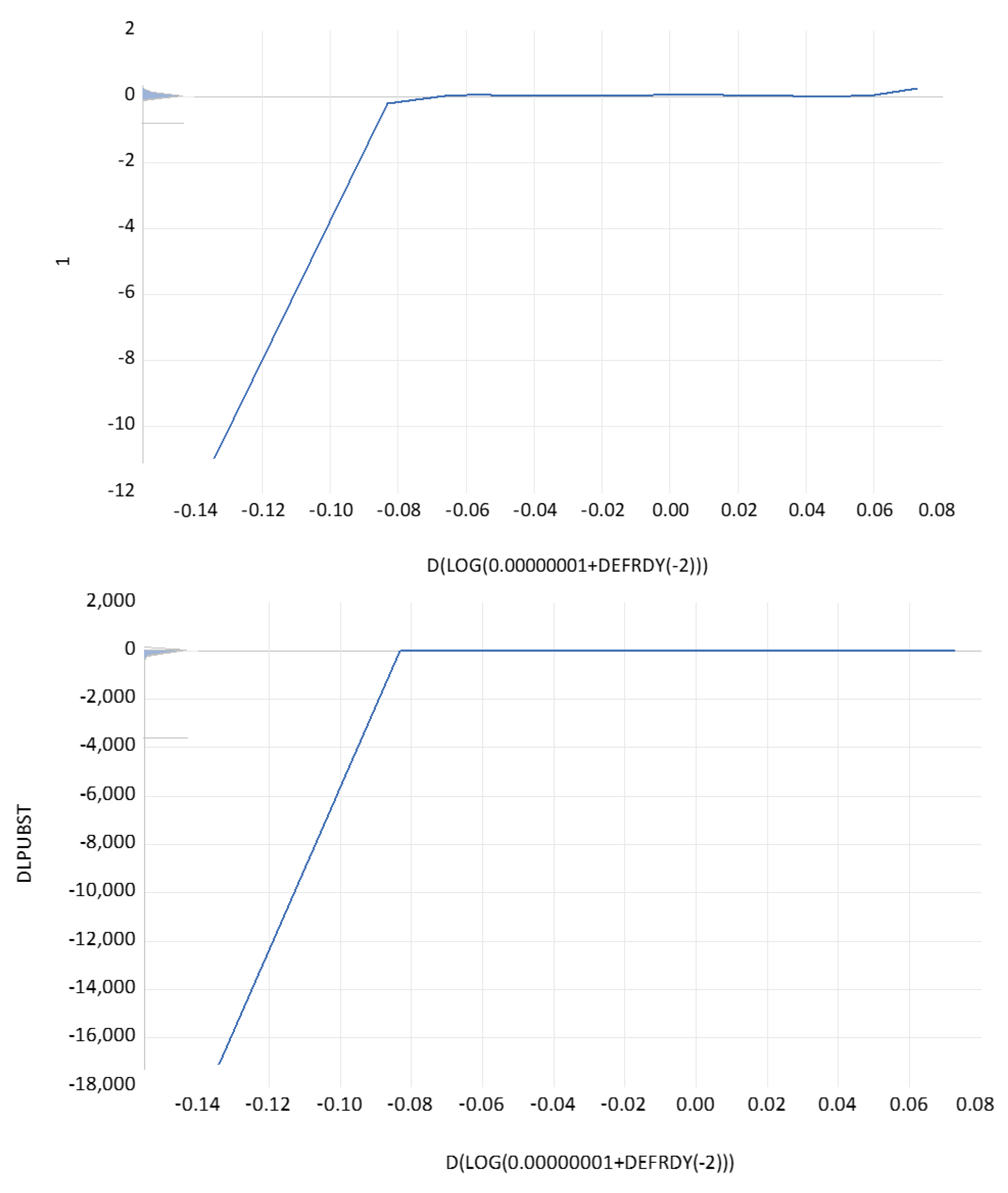
Figure A13.
The partial contribution of foreign BERD stock growth to the regression coefficients of private R&D depending on public R&D in country-year format. Notes. Dependent variable: DLBERDST. Method: Functional coefficients. Sample (adjusted): 1976–2021. Included observations: 1135 after adjustments. Functional coefficient series: DLFBERDST(−3). Kernel: Epanechnikov. Local polynomial degree: 3. Bandwidth: 0.3797 (automatic: CV). Localization grid: Functional coefficient series.
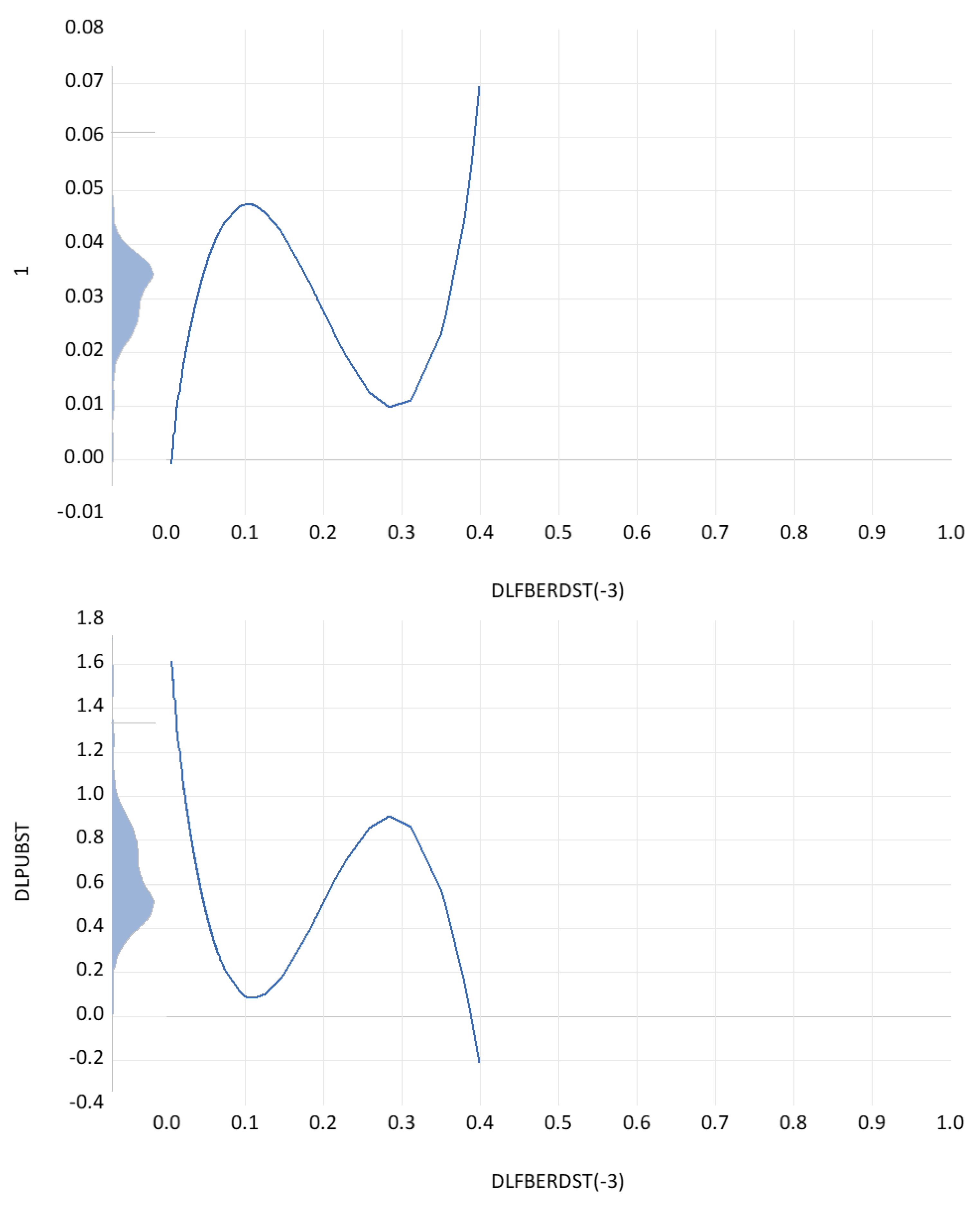
Figure A14.
The partial contribution of GDP four-year average growth rates to the regression coefficients of private R&D depending on public R&D in country-year format. Notes. Dependent variable: DLBERDST. Method: Functional coefficients. Sample (adjusted): 1976 to 2021. Included observations: 1155 after adjustments. Functional coefficient series: SUMG4. Kernel: Epanechnikov. Local polynomial degree: 7. Bandwidth: 0.1000 (automatic: CV). Localization grid: Functional coefficient series.
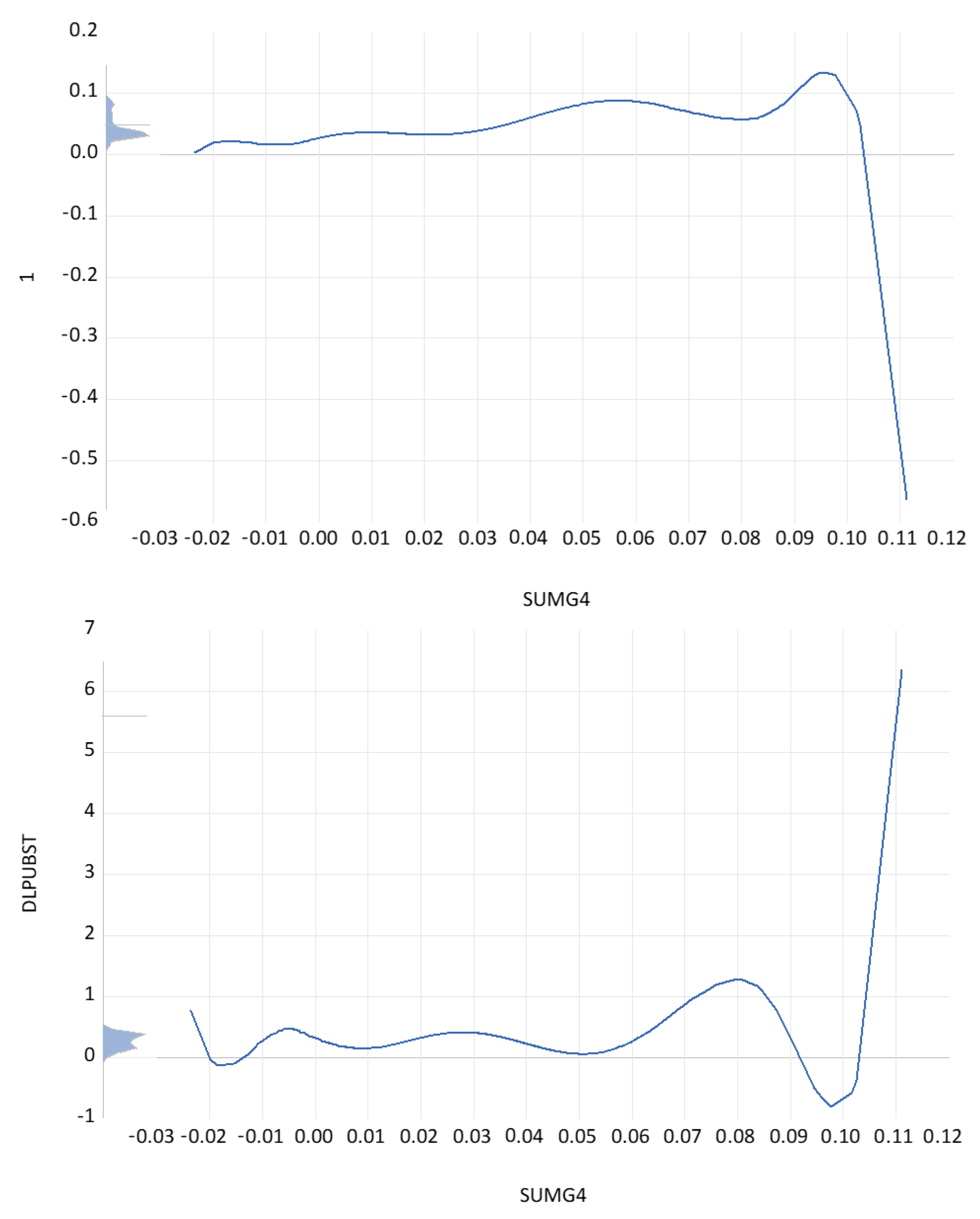
Figure A15.
The partial contribution of lagged BERD stock growth, dlberdst(−2), to the regression coefficients of private R&D depending on public R&D in country-year. Notes. Dependent variable: DLBERDST. Method: Functional coefficients. Sample (adjusted): 1978–2021. Included observations: 1125 after adjustments. Functional coefficient series: DLBERDST(−2). Kernel: Epanechnikov. Local polynomial degree: 3. Bandwidth: 0.4595 (automatic: CV). Localization grid: Functional coefficient series.
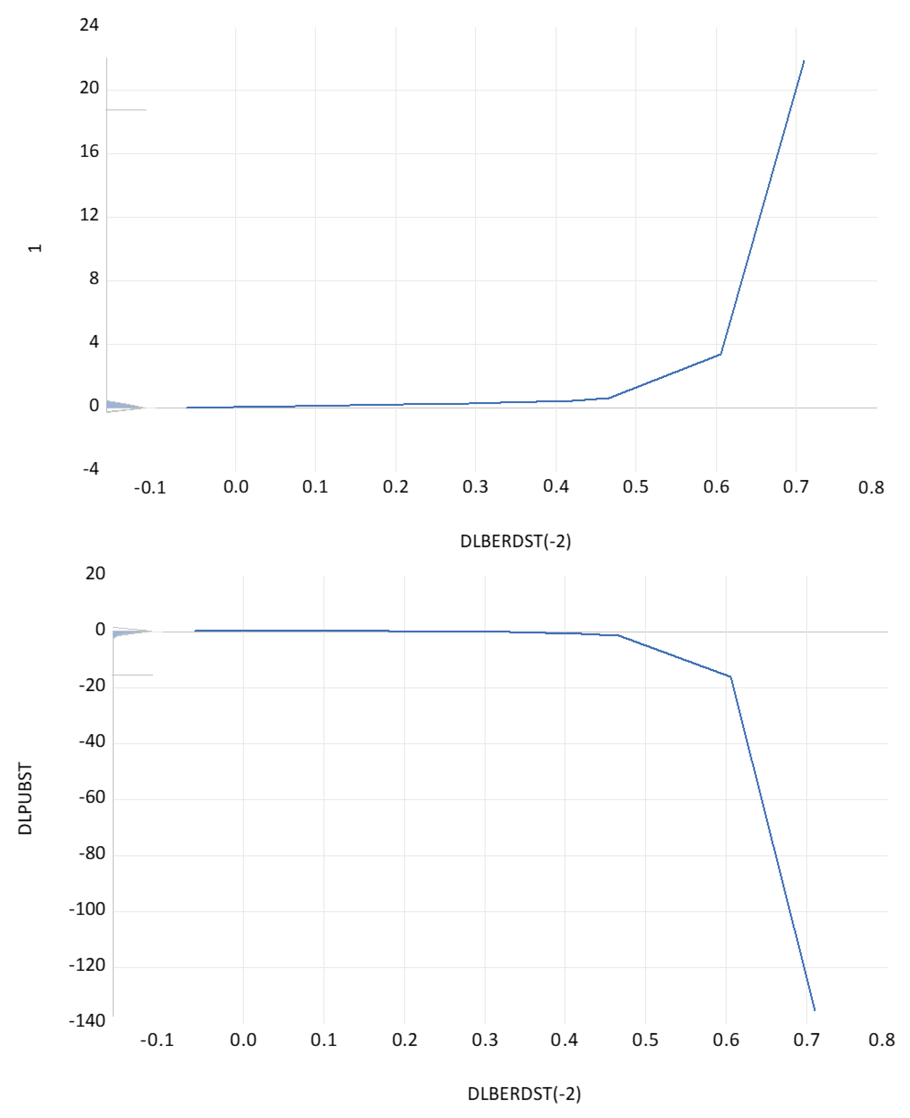
Appendix C. From Partial to Total Coefficients
Given countries index i, periods index t, regressors of (1b) with index k = 1, …, 6 (=K), and functional series index j = 1, …, 7 in line with the first seven rows of Table 17, the estimated regression coefficients are
Upper index (0) is for the constants, (1a) is for the linear terms, and (2a) is for the quadratic terms, corresponding to the exponent of the polynomial term. The coefficients denoted as correspond to those in the main text but include the term 1/L!. Cai et al. (2000), several articles, and the EViews manual focus on the linear case and ignore the quadratic and higher terms, and add kernel weights, which are not visible in the graphs of Figure A1, Figure A2, Figure A3, Figure A4, Figure A5, Figure A6, Figure A7, Figure A8, Figure A9, Figure A10, Figure A11, Figure A12, Figure A13, Figure A14 and Figure A15. They write the formulas for the least squares minimization problem. We write them in line with the regression output.
The right-hand side of the equation has one line for each functional series index j = 1, …, 7. The numerical value of this line is part of the regression output. It has a panel structure with index it, as can be seen from both sides of the equation. Summing over these values for each observation it yields the coefficients on the left-hand side of the equation. In sum, the left-hand side is the functional coefficient for regressor k of observation it, which equals the sum of the contributions of the seven functional series on the right-hand side of the equation, which in turn consists of the seven single contributions written in each line for the contribution of one functional series. Appendix E below on observation Ireland 2019 (related to Figure 3) illustrates the numerical working of the procedure.
The least squares estimator of the coefficients on the right-hand side of the above equation, with variables on the right-hand side abbreviated as Zi taken from Fan and Zhang (2000) for only one functional series, is
with
We have abstained from putting vertical dots between rows 11, it, and NT for reasons of space. Terms below underbrace indicate the number of rows and columns of the matrices. With only one functional series, for each of the K regressors, there are q + 1 terms in the Taylor approximation of a polynomial of degree q, with q = 2 for the quadratic case. In other words, for q = 2, the coefficient estimators a(z) shown here are the first three coefficients in the formula for ak, it above and for each k = 1,…, K.
In addition to the information on estimated functional coefficients in Table 18, we present the kernel density distribution for all eight coefficients. The graphs show that the data are highly concentrated in the middle and much more so than the functional series data in Appendix A. There is little support at the extreme ranges. Still, the concentration in the middle is broad enough to allow coefficient variation.
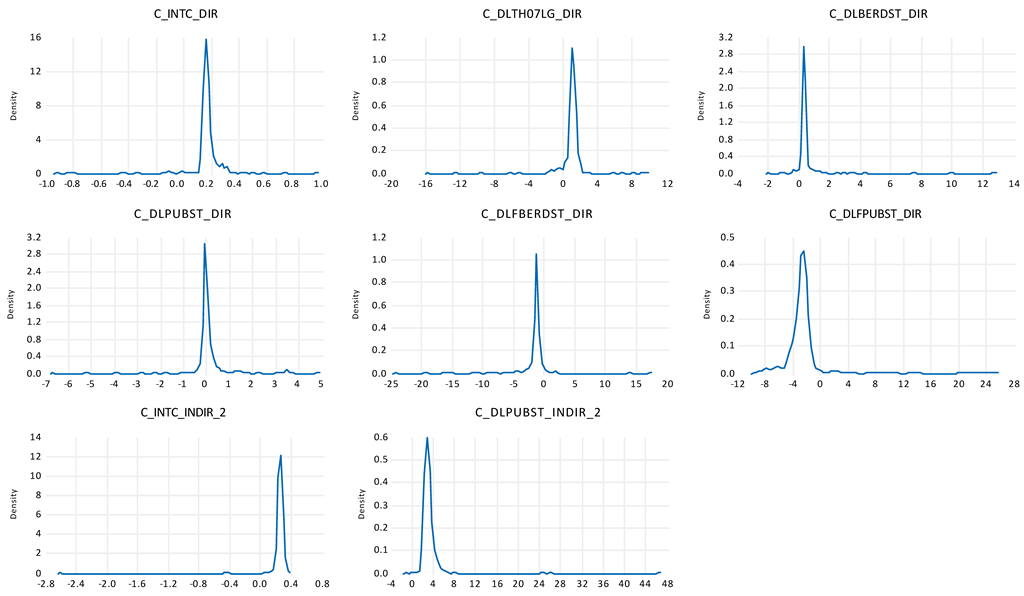
Appendix D. Derivation of Confidence Intervals for Figure 3: The Sum of Direct and Indirect Effects of Public R&D
We need the variance and standard errors of c(4) + c(3)c(8), the sum of the direct and indirect effects. To do this calculation, we need the variances of c(4), the direct effect of public R&D, and the variance of c(3)xc(8), the indirect effect of public R&D. We calculate the variance of c(3)*c(8) using the delta method (see Greene, 2012). The variance of an expression f, which is a function of two estimated parameters b and c, f(b, c), can be calculated as follows (Greene, 2012).
In our case, f = c(3)c(8), b = c(3), c = c(8), var(b) = var(c(3)) = 1.198628021050654, var(c) = var(c(8)) = 7.828961751565975, cov(b,c) = cov(c,b) = cov(c(3),c(8)) = 0.6388582876304415. Insertion of these formulas and numbers (abbreviated here, but not in later calculations) into the variance formula yields
Doing the multiplication, we get
The variance of the total effect with var(c(4)) = 0.4177436715726263 is then var(c(4) + c(3)c(8)) = var(c(4)) + var(c(3)c(8)) + 2cov(c(4), c(3)c(8)) = 0.418 + 1.199c(8)c(8) + 0.64c(3)c(8) + 0.64c(8)c(3) + 7.83c(3)c(3) + 2(−2.157215282462584).
The standard errors then are SE = (var(c(4) + c(3)c(8)))1/2, leading to a confidence interval of c(4) + c(3)c(8) ± 1.96SE.
As the parameter values have a panel structure, the variances, standard errors, and confidence bands as calculated using the delta method also have a panel structure of values.
As a remark of caution, we like to emphasize that each of the three coefficients in the expression c(4) + c(3)xc(8) is a sum of the contributions of the functional series. Each of these contributions has its own confidence interval based on a polynomial two degrees higher than the polynomial used for the contribution. This degree is often very high, as indicated in the tables.
It would be preferable to use the long-run (co)variances with degrees of freedom adjustment, Bartlett kernel, and Newey–West HAC (fixed or automatic), or any of the alternatives (all without pre-whitening; with or without ‘truncation to integer’). However, none of the combinations can be reproduced with the same choices in Eviews14 a moment later, although identifiers are by explicit year and country code. The differences are not minor but rather large percentages. Fixing the bandwidth does not help: NW fixed is also doing that; bandwidth 4 and lag length 2 are also not reproducible a moment later. For c(3)*c(8), we get 405 estimates. With small average T = 19.3 and small N = 21, and cross-section dependence in the coefficients, convergence problems for the long-run covariance happen to occur. Therefore, we use the empirical covariance matrix with degree of freedom adjustment; this is somewhat unsatisfactory because we lose the HAC. In short, we could not use the HAC method; it is an open question whether this makes the confidence intervals wider or less so and, therefore, adds additional uncertainty regarding the confidence interval.
Appendix E. On Observation Ireland 2019
Observation Ireland 2019 is deleted when making Figure 3 because it is very large. A reviewer has suggested investigating it in detail. We do so using Table A1 and Table A2 below. The first part of Table A1 shows that the data for the regression of the productivity function (1b) and the first-order conditions (5) have nothing that is unusual. There are two data points with absolute values above 20 percent (appearing three times because of the lags); and there are only two other data points with values slightly above ten percent. They appear in the lagged dependent variables and in the service share. In particular, the growth rates were remarkably high in Ireland in 2015, 26%, when coming out of the crisis, and this decreases the share of services. This would not suggest taking these data points out as outliers.
Table A1.
Data information on observations ‘Ireland 2015–2019’.
The coefficient that is dropped from Figure 3 is C(3)xC(8) + C(4) = 332.94 for Ireland 2019. This coefficient is disentangled in Table A2. From the rows ‘sum: funct. coeff’ in Table A2, we see C(3) = 12.755, C(4) = −1.785, and C(8) = 26.234. C(8) is the largest of all functional coefficients for Ireland 2019, followed by C(6); its largest contribution comes from D(LOG(SRVY(−4))), 23.397. C(3) = 12.755 is roughly in the middle of all values in Table A2; its largest contribution comes from D(LOG(GDP(−5)/(LF(−5)))), 12.565. The product C(3)xC(8) = 334.7 is extremely high because the highest term and a medium-sized term are multiplied. Having high, medium, and low values of functional coefficient contributions is the natural consequence of not having constant coefficients. This coefficient is, of course, high, but it is there only for one year in one country, in post-crisis time; it can be traced to high growth in 2015, followed and preceded by low and even negative growth (see rows DLTH07(−2)), D(LOG(SRVY)), and D(LOG(SRVY(−3))) in Table A1).
In terms of Appendix C, the notation for C(1)–C(8) for Ireland 2019 is ak, 12,61, with k = 1,…, 8, i = 12 as the index for Ireland and t = 61 as the period 2019 (1959–2019). C(3)*C(8) then translates into a3, 12,61 ∗ a8, 12,61.
Table A2.
Functional coefficient contributions of smoothing variables, Ireland 2019 (a).
Notes
| 1 | van Daal and Merkies (1985) summarize the history of economic thinking. |
| 2 | Park (1998) and Herzer (2022) specify slightly different models of direct and indirect effects. |
| 3 | Ziesemer (2021b) relates this function to the literature on utility and production functions. |
| 4 | The literature of this paragraph discusses other nonlinear functions as alternatives to polynomials, such as (−0.6 − 1.25x)e^{−4x2}. Eviews selects only the polynomials as a procedure, which is based on Cai et al. (2000). |
| 5 | Interesting economic examples are the average rate of return over some periods (J. Z. Huang & Shen, 2004; example 2); distance from TFP frontier, A − Af < 0 (Goñi & Maloney, 2017). |
| 6 | The linear case of b(Z)X, therefore, has some similarity with interaction effects in parametric methods. There, quadratic and cubic polynomials would often run into the ‘near singular matrix’ warning, though. They are special cases that suppress nonlinearities from higher polynomial degrees. Threshold models impose a low number of ranges for which the slopes differ; they could be tested against functional coefficient models, but with several regressors with such ranges, this can be rather cumbersome; in the simple case of Z = X, the definition of a threshold as having different coefficients on each side of the threshold value X* holds for each X, meaning that Z = X yields, in principle, a continuum of thresholds, but not all estimation techniques and statistics will work for many thresholds. Rolling windows lead to even smaller (sub-) samples with little guidance for the window size. Still, another heterogeneous alternative is the use of slope dummies suggested by Brock and Durlauf (2001); the group of N countries is disaggregated into n << N groups for which a dummy multiplied by the slope coefficients is employed in addition to the basic coefficient, leading to n coefficients rather than only one; this leaves more observations for the non-dummy observation compared to the method of splitting the sample. As indicated above, factor models with country-specific coefficients are another advanced way of dealing with heterogeneity and bias from unobserved omitted variables and cross-section dependence. Given the limited length of our data, thresholds, knots of spline-based nonlinear models, and rolling windows would not lead to more exact estimation than functional coefficient series. |
| 7 | dlfpubst(−3) has constant coefficients when using a polynomial of degree 4, but not for a linear one. |
| 8 | For countries without defense R&D, the log does not exist. Therefore, we have added a small number to the defense R&D variable. As for the zero observations, we have log(0) = −∞, meaning that it does not exist without adding anything; adding unity, as is often found in the literature, leads to log(1 + 0) = 0, which is indeed a big difference when using it in regressions; using instead log(0.00000001) = −18.4207, which is strongly negative, is an economic nonlinearity going into the variable definition. Dropping zero variables takes the alternative out, which is even more unsatisfactory. An alternative to adding 1/10j, j = …, −2,−1, 0, 1, 2, …. is the formula log(x + (x2 + 1)0.5) taken from Busse and Hefeker (2007); replacing 1 by 1/10j in this formula still allows this formula to work, and it is thereby also not unique. The Results, of course, only hold for the specification used, and there is no claim for generalization here. |
| 9 | One economic reason may be that with a unit root Z would only change with accumulated residuals once Z(0) is given. This would imply that coefficients are explained by random walks, which could be of limited economic interest, unless emphasis is on an included time trend or the cross-section differentiation of Z(0). |
| 10 | Econometric endogeneity discussed in this paragraph deals with the estimation bias from correlation of regressors and residuals. The word ’endogenous’ in the title of this article refers to the basic deterministic math definition saying that a variable depends on other variables, as in the functional coefficient notion of changing coefficients. |
| 11 | Data for service/GDP ratios of Taiwan are from https://eng.stat.gov.tw/ (accesed on 28 November 2024). |
| 12 | See Cai et al. (2000). These values can be downloaded after estimation. In the quadratic case, for example, we get one number per country-year combination for each of the regression coefficients of (1b). It is the linear–quadratic combination of coefficients with linear and quadratic variables. |
| 13 | Eviews avoids the issue of false positives from multiple testing through the use of bootstrapping as in Fan and Zhang (2000). |
| 14 | We have also explored the effect of the average growth rates of the last four years, but this only has an effect on the indirect effect shown below. |
| 15 | Method: Panel least squares. Sample (adjusted): 1968 to 2019. Periods included: 52. Cross-sections included: 21. Total panel (unbalanced) observations: 680. Period SUR (PCSE), standard errors, and covariance (d.f. corrected). Cross-section fixed (dummy variables). Period fixed (dummy variables). The corresponding p-values are 1.989 × 10⁻²²; 0.006; 1.169 × 10−08; and 0.055. Adj. R-sq.: 0.36. Durbin–Watson stat: 2.029. Adj. R-sq is lower when cross-section GLS weights are used instead of period fixed effects. When service shares are constant, the long-run rate of technical change is obtained as 0.009/(1 − 0.147) = 0.011. |
| 16 | See Cai et al. (2000) for an exact but lengthy and complicated formulation. |
| 17 | Note the similarity with the Lucas critique in macroeconomics. Functional coefficient regression is a method that can handle it to some extent when testing whether a policy variable changes regression coefficients. |
| 18 | A highly nonlinear function that could be tested is T = F(G(B,B*), H(P,P*)), where F, G, and H are all CES functions. The equality of marginal products of B and P would leave foreign R&D variables in the first-order equation. This would require a paper on its own, though, as the current one is already extraordinarily long. |
| 19 | Null: Unit root (assumes individual unit root process). Tests by Im, Pesaran, Shin W-stat, ADF Fisher chi-square, and PP Fisher chi-square. |
| 20 | The confidence intervals of this figure are derived using the delta method in ‘Appendix D’. |
References
- Ahn, S. C., & Horenstein, A. R. (2013). Eigenvalue ratio test for the number of factors. Econometrica, 81(3), 1203–1227. [Google Scholar] [CrossRef] [Scilit]
- Archibugi, D., & Filippetti, A. (2018). The retreat of public research and its adverse consequences on innovation. Technological Forecasting & Social Change, 127, 97–111. [Google Scholar] [CrossRef] [Scilit]
- Bernard, A. B., & Jones, C. I. (1996). Technology and convergence. The Economic Journal, 106(437), 1037–1044. [Google Scholar] [CrossRef] [Scilit]
- Boppart, T. (2014). Structural change and the Kaldor facts in a growth model with relative price effects and non-Gorman preferences. Econometrica, 82(6), 2167–2196. [Google Scholar] [CrossRef] [Scilit]
- Boppart, T., & Weiss, F. J. (2013). Non-homothetic preferences and industry directed technical change (Working Paper 123). University of Zurich, Department of Economics. [Google Scholar]
- Boysen-Hogrefe, J. (2025). Is the supermultiplier currently nil?—A replication study of Deleidi and Mazzucato (2021). Research Policy, 54(3), 105176. [Google Scholar] [CrossRef] [Scilit]
- Brock, W. A., & Durlauf, S. N. (2001). What have we learned from a decade of empirical research on growth? Growth empirics and reality. The World Bank Economic Review, 15(2), 229–272. [Google Scholar] [CrossRef] [Scilit]
- Busse, M., & Hefeker, C. (2007). Political risk, institutions and foreign direct investment. European Journal of Political Economy, 23(2), 397–415. [Google Scholar] [CrossRef] [Scilit]
- Cai, Z. (2003). Trending time-varying coefficient models with serially correlated errors (SFB 373 Discussion Paper No. 2003, 7). Humboldt University of Berlin. [Google Scholar]
- Cai, Z., Chen, L., & Fang, Y. (2015). Semiparametric estimation of partially varying-coefficient dynamic panel data models. Econometric Reviews, 34(6–10), 695–719. [Google Scholar] [CrossRef] [Scilit]
- Cai, Z., Fan, J., & Yao, Q. (2000). Functional-coefficient regression models for nonlinear time series. Journal of the American Statistical Association, 95(451), 941–956. [Google Scholar] [CrossRef] [Scilit]
- Cai, Z., Fang, Y., & Xu, Q. (2022). Testing capital asset pricing models using functional-coefficient panel data models with cross-sectional dependence. Journal of Econometrics, 227(1), 114–133. [Google Scholar] [CrossRef] [Scilit]
- Cai, Z., Li, Q., & Park, J. Y. (2009). Functional-coefficient models for nonstationary time series data. Journal of Econometrics, 148(2), 101–113. [Google Scholar] [CrossRef] [Scilit]
- Cantner, U., Graf, H., Prytkova, E., & Vannuccini, S. (2018). The compositional nature of productivity and innovation slowdown (Jena Economic Research Papers 2018-006). Friedrich Schiller University Jena. [Google Scholar]
- Cantner, U., & Guerzoni, M. (2009). Innovation driving industrial dynamics. Between incentives and knowledge. Economia Politica, 3, 481–510. [Google Scholar] [CrossRef] [Scilit]
- Castellacci, F., & Archibugi, D. (2008). The technology clubs: The distribution of knowledge across nations. Research Policy, 37(10), 1659–1673. [Google Scholar] [CrossRef] [Scilit]
- Castellacci, F., & Natera, J. M. (2013). The dynamics of national innovation systems: A panel cointegration analysis of the coevolution between innovative capability and absorptive capacity. Research Policy, 42(3), 579–594. [Google Scholar] [CrossRef] [Scilit]
- Chen, R., & Tsay, R. S. (1993). Functional-coefficient autoregressive models. Journal of the American Statistical Association, 88(421), 298–308. [Google Scholar] [CrossRef] [Scilit]
- Ciaffi, G., Deleidi, M., & Di Bucchianico, S. (2024). Stagnation despite ongoing innovation: Is R&D expenditure composition a missing link? An empirical analysis for the US (1948–2019). Technological Forecasting & Social Change, 206, 123575. [Google Scholar] [CrossRef] [Scilit]
- Coccia, M. (2010). Public and private investment in R&D: Complementary effects and interaction with productivity growth. European Review of Industrial Economics and Policy. Available online: https://hal.science/hal-03468720 (accessed on 1 July 2024).
- Comin, D. A., Lashkari, D., & Mestieri, M. (2025). The structural transformation of innovation (NBER Working Paper 33855). National Bureau of Economic Research. [Google Scholar]
- Deleidi, M., & Mazzucato, M. (2021). Directed innovation policies and the supermultiplier: An empirical assessment of mission-oriented policies in the US economy. Research Policy, 50, 104151. [Google Scholar] [CrossRef] [Scilit]
- Denison, E. (1962). The sources of economic growth in the United States. Committee for Economic Development. [Google Scholar]
- Dosi, G. (1988). Sources, procedures, and microeconomic effects of innovation. Journal of Economic Literature, 26, 1120–1171. [Google Scholar]
- Durlauf, S. N., Johnson, P. A., & Temple, J. R. (2005). Growth econometrics. Handbook of Economic Growth, 1, 555–677. [Google Scholar] [CrossRef] [Scilit]
- Eberhardt, M., & Teal, F. (2013). No mangoes in the tundra: Spatial heterogeneity in agricultural productivity analysis. Oxford Bulletin of Economics and Statistics, 75(6), 914–939. [Google Scholar] [CrossRef] [Scilit]
- Fan, J., & Zhang, W. (2000). Simultaneous confidence bands and hypothesis testing invarying-coefficient models. Scandinavian Journal of Statistics, 27, 715–731. [Google Scholar] [CrossRef] [Scilit]
- Fan, J., & Zhang, W. (2008). Statistical methods with varying coefficient models. Statistics and Its Interface, 1, 179–195. [Google Scholar] [CrossRef] [Scilit] [PubMed]
- Fernald, J., Inklaar, R., & Ruzic, D. (2025). The productivity slowdown in advanced economies: Common shocks or common trends? Review of Income and Wealth, 71(1), e12690. [Google Scholar] [CrossRef] [Scilit]
- Fieldhouse, A. J., & Mertens, K. (2023). The returns to government R&D: Evidence from U.S. appropriations shocks. Federal Reserve Bank of Dallas. [Google Scholar]
- Goel, R. K., Payne, J. E., & Ram, R. (2008). R&D expenditures and U.S. economic growth: A disaggregated approach. Journal of Policy Modeling, 30, 237–250. [Google Scholar] [CrossRef] [Scilit]
- Goñi, E., & Maloney, W. F. (2017). Why don’t poor countries do R&D? Varying rates of factor returns across the development process. European Economic Review, 94, 126–147. [Google Scholar] [CrossRef] [Scilit]
- Greene, W. H. (2012). Econometric analysis (7th ed.). Pearson Education. [Google Scholar]
- Guellec, D., & Van Pottelsberghe de la Potterie, B. (2003). The impact of public R&D expenditure on business R&D. Economics of Innovation and New Technology, 12, 225–243. [Google Scholar] [CrossRef] [Scilit]
- Haavelmo, T. (1954). A Study in the theory of economic evolution. North Holland. [Google Scholar]
- Hall, B. H., Mairesse, J., & Mohnen, P. (2010). Measuring the returns to R&D. In B. H. Hall, & N. Rosenberg (Eds.), Handbook of the economics of innovation (pp. 1033–1082). North Holland. [Google Scholar]
- Hastie, T., & Tibshirani, R. (1993). Varying-coefficient models. Journal of the Royal Statistical Society Series B: Statistical Methodology, 55(4), 757–779. [Google Scholar] [CrossRef] [Scilit]
- Henderson, D. J., Rodriguez-Poo, J. M., Soberon, A., & Wang, T. (2026). Estimation of functional coefficient panel data models with endogenous selectivity and fixed effects: A pairwise approach. Economics Letters, 266, 113036. [Google Scholar] [CrossRef] [Scilit]
- Herrendorf, B., Rogerson, R., & Valentinyi, A. (2014). Growth and structural transformation. Handbook of Economic Growth, 2, 855–941. [Google Scholar] [CrossRef] [Scilit]
- Herzer, D. (2022). An empirical note on the long-run effects of public and private R&D on TFP. Journal of the Knowledge Economy, 13(4), 3248–3264. [Google Scholar] [CrossRef] [Scilit]
- Huang, C. Y., Lai, C. C., & Peretto, P. F. (2025). Public R&D, private R&D and growth: A Schumpeterian approach. Journal of Economic Behavior & Organization, 236, 107087. [Google Scholar] [CrossRef] [Scilit]
- Huang, J. Z., & Shen, H. (2004). Functional coefficient regression models for non-linear time series: A polynomial spline approach. Scandinavian Journal of Statistics, 31(4), 515–534. [Google Scholar] [CrossRef] [Scilit]
- Jaumotte, F., & Pain, N. (2005). Innovation in the business sector (OECD Economics Department Working Paper, No. 459). OECD. [Google Scholar]
- Juhl, T. (2005). Functional-coefficient models under unit root behaviour. Econometrics Journal, 8, 197–213. [Google Scholar] [CrossRef] [Scilit]
- Jusélius, K. (2006). The cointegrated VAR model: Methodology and application. Oxford University Press. [Google Scholar]
- Luintel, K. B., & Khan, M. (2004). Are international R&D spillovers costly for the United States? The Review of Economics and Statistics, 86, 896–910. [Google Scholar] [CrossRef] [Scilit]
- Mamuneas, T. P., Savvides, A., & Stengos, T. (2006). Economic development and the return to human capital: A smooth coefficient semiparametric approach. Journal of Applied Econometrics, 21(1), 111–132. [Google Scholar] [CrossRef] [Scilit]
- Moretti, E., Steinwender, C., & Van Reenen, J. (2025). The intellectual spoils of war? Defense R&D, productivity, and international spillovers. The Review of Economics and Statistics, 107(1), 14–27. [Google Scholar] [CrossRef] [Scilit]
- Mowery, D. C., & Rosenberg, N. (1989). Technology and the pursuit of economic growth. Cambridge University Press. [Google Scholar]
- Nakamura, A., & Nakamura, M. (1998). Model specification and endogeneity. Journal of Econometrics, 83(1–2), 213–237. [Google Scholar] [CrossRef] [Scilit]
- Nelson, R. R. (1968). A “diffusion” model of international productivity differences in manufacturing industry. The American Economic Review, 58(5), 1219–1248. [Google Scholar]
- Nelson, R. R. (Ed.). (1993). National innovation systems: A comparative analysis. Oxford University Press. [Google Scholar]
- OECD. (2017). The impact of R&D investment on economic performance: A review of the econometric evidence. In Working party of national experts on science and technology indicators (DSTI/STP/NESTI 2017 12). OECD Publishing. [Google Scholar]
- Park, W. G. (1995). International spillovers of R&D investment and OECD economic growth. Economic Inquiry, 33, 571–591. [Google Scholar] [CrossRef] [Scilit]
- Park, W. G. (1998). A theoretical model of government research and growth. Journal of Economic Behavior & Organization, 34, 69–85. [Google Scholar] [CrossRef] [Scilit]
- Pesaran, M. H. (2015). Time series and panel data econometrics. Oxford University Press. [Google Scholar]
- Rodriguez-Poo, J. M., & Soberon, A. (2014). Direct semi-parametric estimation of fixed effects panel data varying coefficient models. The Econometrics Journal, 17(1), 107–138. [Google Scholar] [CrossRef] [Scilit]
- Schultz, T. W. (1964). Transforming traditional agriculture. Yale University Press. [Google Scholar]
- Soete, L., Verspagen, B., & Ziesemer, T. H. W. (2020). The productivity effect of public R&D in the Netherlands. Economics of Innovation and New Technology, 29(1), 31–47. [Google Scholar] [CrossRef] [Scilit]
- Soete, L., Verspagen, B., & Ziesemer, T. H. W. (2022). The economic impact of public R&D: An international perspective. Industrial and Corporate Change, 31(1), 1–18. [Google Scholar] [CrossRef] [Scilit]
- Solodoha, E., Rosenzweig, S., & Harel, S. (2023). Incentivizing angels to invest in start-ups: Evidence from a natural experiment. Research Policy, 52(1), 104634. [Google Scholar] [CrossRef] [Scilit]
- Sun, Y., Carroll, R. J., & Li, D. (2009). Semiparametric estimation of fixed effects panel data models with smooth coefficients. Advances in Econometrics, 25, 101–129. [Google Scholar] [CrossRef] [Scilit]
- Sveikauskas, L. (2007). R&D and productivity growth: A review of the literature (Working Paper 408). U.S. Bureau of Labor Statistics. [Google Scholar]
- Temple, J. (1999). The new growth evidence. Journal of Economic Literature, 37(1), 112–156. [Google Scholar] [CrossRef] [Scilit]
- Tu, Y., & Wang, Y. (2022). Spurious functional-coefficient regression models and robust inference with marginal integration. Journal of Econometrics, 229(2), 396–421. [Google Scholar] [CrossRef] [Scilit]
- Ullah, A., & Pagan, A. (1999). Nonparametric econometrics. Cambridge University press. [Google Scholar]
- van Daal, J., & Merkies, A. H. Q. M. (1985). The problem of aggregation of individual economic relations; consistency and representativity in a historical perspective. In Measurement in economics: Theory and applications of economics indices (EUR Report 8542/A). Springer. [Google Scholar]
- Van Elk, R., ter Weel, B., van der Wiel, K., & Wouterse, B. (2019). Estimating the returns to public R&D investments: Evidence from production function models. De Economist, 167, 45–87. [Google Scholar] [CrossRef] [Scilit]
- Van Elk, R., Verspagen, B., ter Weel, B., van der Wiel, K., & Wouterse, B. (2015). A macroeconomic analysis of the returns to public R&D investments (CPB DP 313). UNU-MERIT. [Google Scholar]
- Wang, T., & Henderson, D. J. (2022). Estimation of a varying coefficient, fixed-effects Cobb–Douglas production function in levels. Economics Letters, 213, 110354. [Google Scholar] [CrossRef] [Scilit]
- Wang, Y., & Phillips, P. C. (2025). Limit theory for local polynomial estimation of functional coefficient models with possibly integrated regressors. Journal of Econometrics, 249, 106007. [Google Scholar] [CrossRef] [Scilit]
- Zhao, Y. Y., Ge, L. L., & Zhang, K. S. (2025). Semiparametric estimation of a principal functional coefficient panel data model with cross-sectional dependence and its application to cigarette demand. Journal of Statistical Planning and Inference, 236, 106244. [Google Scholar] [CrossRef] [Scilit]
- Ziesemer, T. H. W. (2021a). Mission-oriented R&D and growth. Journal of Applied Economics, 24(1), 460–477. [Google Scholar] [CrossRef] [Scilit]
- Ziesemer, T. H. W. (2021b). Semi-endogenous growth models with domestic and foreign private and public R&D linked to VECMs. Economics of Innovation and New Technology, 30(6), 621–642. [Google Scholar] [CrossRef] [Scilit]
- Ziesemer, T. H. W. (2021c). The effects of R&D subsidies and publicly performed R&D on business R&D: A survey. Hacienda Publica Espanola/Review of Public Economics, 236, 171–205. [Google Scholar] [CrossRef] [Scilit]
- Ziesemer, T. H. W. (2023). Labour-augmenting technical change data for alternative elasticities of substitution: Growth, slowdown, and distribution dynamics. Economics of Innovation and New Technology, 32(4), 449–475. [Google Scholar] [CrossRef] [Scilit]
- Ziesemer, T. H. W. (2024a). Internal rates of return for public R&D from VECM estimates for 17 OECD Countries. Economic Change and Restructuring, 57, 164. [Google Scholar] [CrossRef] [Scilit]
- Ziesemer, T. H. W. (2024b). Mission-oriented R&D and growth of Japan 1988–2016: A comparison with private and public R&D. Economics of Innovation and New Technology, 33(2), 218–247. [Google Scholar] [CrossRef] [Scilit]
- Ziesemer, T. H. W. (2024c). Public R&D and growth: A dynamic panel VECM data analysis for 14 OECD countries. Economies, 12(8), 216. [Google Scholar] [CrossRef] [Scilit]
- Ziesemer, T. H. W. (2026). A data set for domestic and foreign private and public R&D stocks and labour-augmenting technical change for 44 rich or emerging economies with explorations on panel unit roots, cointegration, growth rate slowdown, and con-or divergence. Economics of Innovation and New Technology. [Google Scholar] [CrossRef] [Scilit]
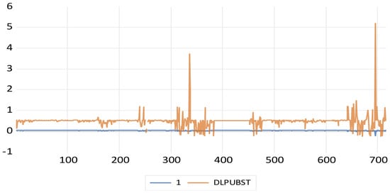
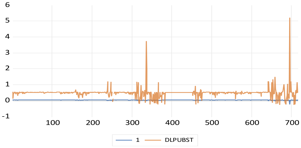
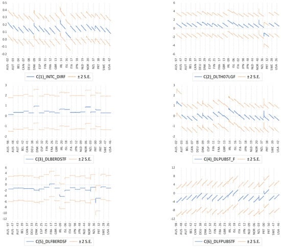
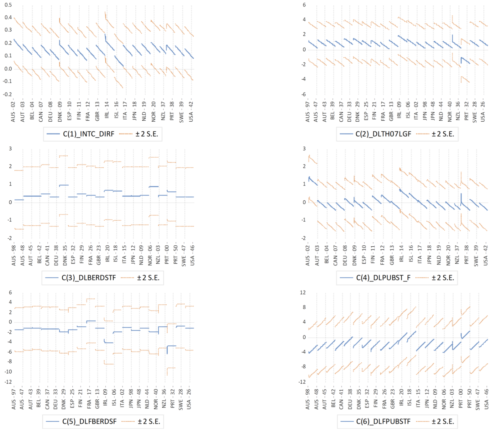
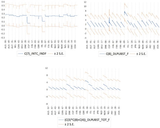
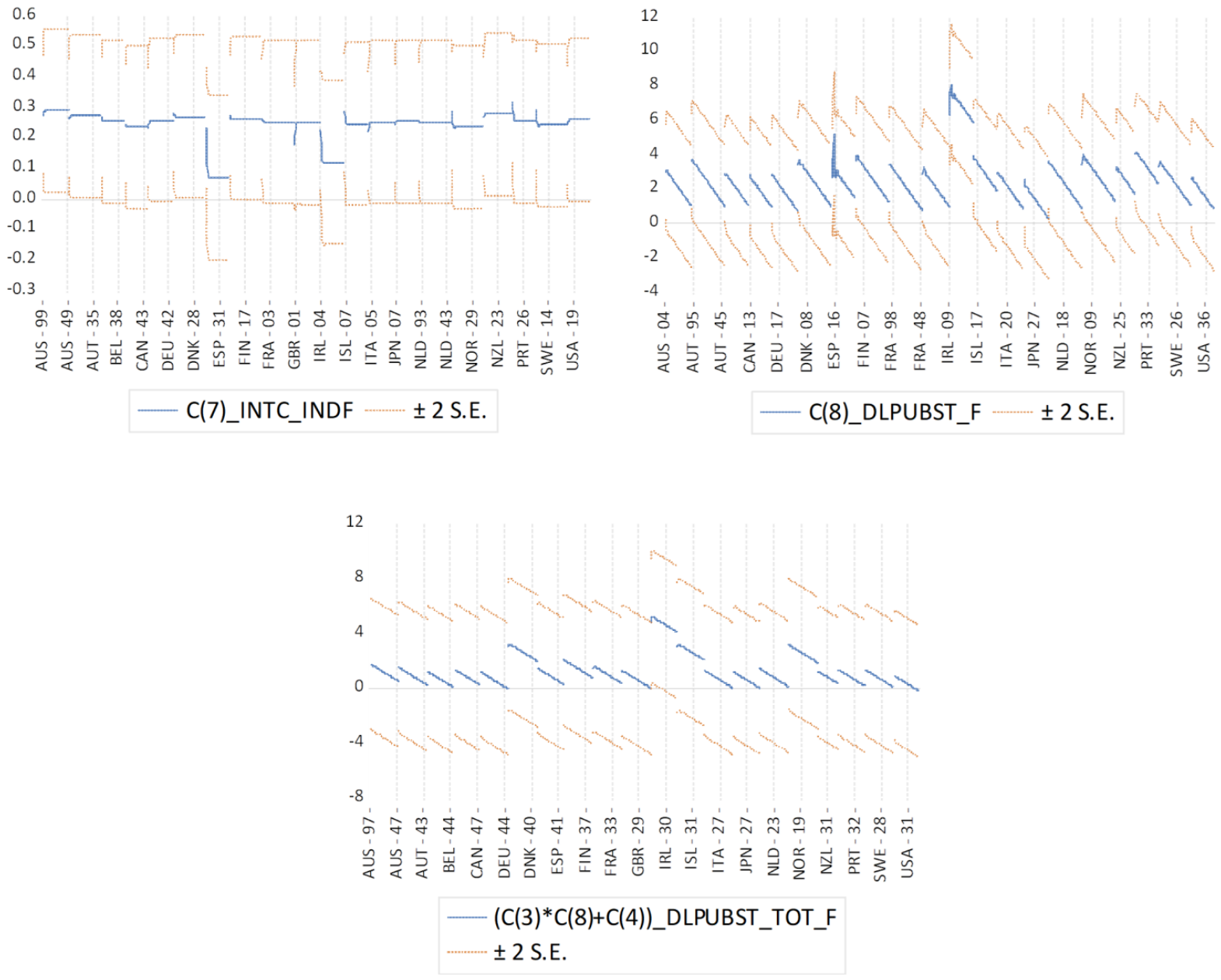

Disclaimer/Publisher’s Note: The statements, opinions and data contained in all publications are solely those of the individual author(s) and contributor(s) and not of MDPI and/or the editor(s). MDPI and/or the editor(s) disclaim responsibility for any injury to people or property resulting from any ideas, methods, instructions or products referred to in the content. |
© 2026 by the author. Licensee MDPI, Basel, Switzerland. This article is an open access article distributed under the terms and conditions of the Creative Commons Attribution (CC BY) license.