Beyond the Nameplate: What Renewable Capacity Targets Do and Do Not Buy in Developing Economies

Abstract

Installed renewable capacity is the leading indicator of energy-transition efforts, yet its conversion into realized generation is rarely estimated directly. This study estimates that rate in a panel of 118 developing and emerging economies over 2001–2023, treating proportional conversion, a unit coefficient, as a testable benchmark. In the preferred two-way fixed-effects specification, non-hydro renewable generation per person rises with one-year-lagged capacity per person, both in log(1 + x) form, at a rate of 1.042 (standard error, SE = 0.029), statistically indistinguishable from proportional conversion (test of unit coefficient, p = 0.148); the pure log–log elasticity among positive observations is lower, 0.845 (SE = 0.039). The estimate is stable under country-specific trends (0.924, SE = 0.046) and fixed technology shares (1.025, SE = 0.029), and a distributed lag in exact first differences shows that generation responds mainly to the current and previous year’s capacity changes, with a cumulative response of 1.070 (SE = 0.044). Higher lagged capacity is associated with a 3.630 percentage-point rise in the renewable output share (SE = 0.813) and a 3.258 percentage-point fall in the fossil share (SE = 0.771). Governance interactions are small and fragile under multiple-testing correction, and Poisson and pure log–log checks address the units-sensitivity of log(1 + x) estimates. Conditional on lag structure and functional form, deployment statistics are informative about realized generation and fossil substitution, whereas broader institutional and development gains remain unconfirmed.

1. Introduction

Installed renewable-energy capacity has become a central indicator of progress in the global energy transition. It is visible, comparable across countries, and closely aligned with Sustainable Development Goal (SDG) indicator 7.b.1, which measures renewable electricity-generating capacity in watts per person (United Nations Statistics Division, 2024). Yet capacity is an input into an electricity system, not an output from it. A megawatt recorded at year-end does not reveal how much electricity the asset generates, whether the grid can absorb its output, whether fossil generation is displaced, or whether households receive more reliable and inclusive service. Whether recorded capacity converts into realized generation, and at what rate, is therefore an empirical parameter with direct measurement consequences, and estimating it credibly in an unbalanced country panel raises familiar applied-econometrics questions of functional form, lag structure, and inference.

This distinction is especially important in developing and emerging economies. Rapid demand growth, limited transmission infrastructure, utility financial constraints, fuel subsidies, uneven regulatory enforcement, and shortages of storage or system flexibility can all widen the distance between physical deployment and usable electricity. Current assessments likewise identify grid expansion, system flexibility, permitting, finance, and project bankability as practical constraints on usable renewable output (International Energy Agency, 2024). At the same time, non-hydro technologies such as solar, wind, bioenergy, geothermal, and marine power differ from inherited hydropower systems in age, operating profile, financing structure, and policy context. Treating all renewable capacity as a single stock can therefore obscure the contemporary transition that policymakers are attempting to accelerate.

A large empirical literature studies the determinants of renewable-energy adoption, investment, consumption, or electricity shares. Existing results identify policy instruments, income, energy structure, political conditions, and institutional quality as potential drivers, but they are not uniform across samples or outcomes (Marques et al., 2010; Pfeiffer & Mulder, 2013; Aguirre & Ibikunle, 2014; Polzin et al., 2015; Cadoret & Padovano, 2016; Romano et al., 2017; Uzar, 2020; Rahman & Sultana, 2022). Two adjacent strands come closer to the present question but stop short of it. The first documents that capacity is an imperfect guide to output: capacity factors differ sharply by technology (Bolson et al., 2022), and cross-country renewable-generation efficiency is only weakly aligned with installed-capacity rankings (Li et al., 2022). These studies compare efficiency frontiers or capacity-factor ratios; they do not estimate, within countries and over time, how installed capacity becomes realized generation. The second asks whether renewable output displaces fossil generation, a question posed since York (2012) found displacement to be far less than one-for-one and pursued more recently with first differences and technology disaggregation in high- and middle-income or OECD samples (Liddle, 2024; Karlilar Pata & Balcilar, 2024). These studies take generation as given and estimate its effect on the fossil share; they are not centered on developing economies, and they do not ask whether installed capacity becomes generation in the first place. Neither strand estimates, within countries and over time, the rate at which installed non-hydro capacity becomes generation in developing economies, tests that rate against a proportional benchmark, or follows the same deployment measure through to the electricity mix and to broader system outcomes within one design. The question this paper takes up is therefore whether the deployment statistics used to track transition progress translate systematically into realized generation and a changing electricity mix across a broad panel of developing economies that differ in grids, technology composition, institutions, income, and system constraints.

This paper treats the conversion rate as a parameter to be estimated and tested rather than assumed. The estimation uses a country-year panel assembled from technology-level renewable capacity and generation statistics, World Development Indicators, and the Worldwide Governance Indicators. The headline sample contains 2252 observations from 118 developing and emerging economies over 2001–2023. The preferred outcome is log(1 + x) non-hydro renewable generation per person, and the preferred exposure is one-year-lagged log(1 + x) non-hydro renewable capacity per person. The model includes country and year fixed effects and a parsimonious set of time-varying controls. Government effectiveness is evaluated as a prespecified moderator, with the remaining governance dimensions used in sensitivity tests.

The results establish a clear hierarchy. First, installed non-hydro capacity translates into operational generation at a rate close to one-for-one within countries. The preferred coefficient is 1.042 with a standard error of 0.029; a formal test cannot reject proportional conversion, and the estimate remains close to one across standard-error estimators, lag choices, influential-observation treatments, income groups, and regions. The proportional benchmark holds in the fixed-unit log(1 + x) and Poisson forms and is rejected on the low side in pure logarithms, where the elasticity among positive observations is 0.845 (SE = 0.039). Matched solar and bioenergy relationships are likewise near-proportional, and the wind relationship is once entry from zero capacity is separated from the intensive margin. A distributed lag in exact first differences shows that the response to a capacity change arrives mainly within the year of installation and the year after and cumulates to 1.070 (SE = 0.044), consistent with commissioning lags and the partial-year operation of newly installed assets. Second, and closer to the substitution a transition requires, greater non-hydro capacity is associated with a higher renewable electricity share and a lower fossil electricity share, both robust to multiple-testing correction. Third, the institutional evidence is weak and frequently contrary to the original amplification hypothesis: the government-effectiveness interaction is small and fragile once multiple governance indicators and limited within-country variation are taken into account, alternative governance dimensions are null, and direct conversion-efficiency tests do not survive family-level multiple-testing correction. Finally, the models do not establish improvements in electricity access, transmission losses, or per capita carbon emissions.

The paper contributes in four ways, two substantive and two econometric. First, it traces the energy transition through four stages (deployment, operational generation, electricity-mix substitution, and broader development outcomes) rather than treating installed capacity, the indicator most often used to characterize transition progress, as a complete description of it. Second, it isolates non-hydro renewables and tests matched solar, wind, and bioenergy relationships, so that neither legacy hydropower nor a changing technology mix drives the headline result, and it asks not merely whether conversion is positive but whether it is proportional. Third, on the econometric side, it takes the unit coefficient as a formal null tested by Wald statistics rather than an informal reading of magnitudes, addresses the units-dependence of log(1 + x) estimates with fixed per capita units, an intensive-margin comparison, a pure log–log elasticity, and a Poisson pseudo-maximum-likelihood check, and uses distributed lags in exact first differences to separate the long-run relationship from the timing of the response. It also applies wild cluster restricted bootstrap inference where subgroup models leave few clusters. Fourth, it reports an evidence hierarchy: deployment translates into generation and a changing electricity mix, but broad governance does not robustly moderate that conversion, and the models do not confirm downstream gains in access, losses, or emissions. Relative to the capacity-factor and efficiency comparisons and to the displacement studies cited above, the contribution is therefore the joint estimation, in a single developing-economy panel, of the deployment-to-generation rate, its proportionality, and its electricity-mix counterpart. The practical implication is a measurement lesson: capacity targets and SDG indicator 7.b.1 should be read alongside generation, technology composition, and electricity-mix measures rather than on their own.

The estimates should be interpreted as conditional within-country associations. Country and year fixed effects absorb time-invariant national characteristics and common shocks, but they do not eliminate all time-varying confounding, policy anticipation, measurement error, or simultaneity. Dynamic and internal-instrument exercises are therefore used as diagnostics rather than as a basis for causal claims. The remainder of the paper develops the conceptual framework, describes the data and empirical strategy, presents the results, and discusses their implications for research and policy.

2. Conceptual Framework and Hypotheses

2.1. From Installed Capacity to Operational Generation

Installed capacity measures maximum net generating capability at the end of a period, while generation measures electricity actually produced; the International Renewable Energy Agency (IRENA) reports the two separately and documents cases without matching capacity–production values (International Renewable Energy Agency, 2024). The two should be positively related, but not mechanically one-for-one. Capacity-factor evidence also shows material technology and regional differences in output relative to nameplate capacity (Bolson et al., 2022). Resource quality, technology mix, commissioning dates, outages, curtailment, grid congestion, maintenance, dispatch rules, and demand conditions determine how the installed stock is used. End-of-year capacity includes assets that may have operated for only part of the year, which is one reason the empirical design lags capacity and treats engineering-style capacity-factor ratios only as secondary proxies.

The distinction motivates a direct deployment-to-operation test. Because the distributions contain many small values and strong right tails, the preferred model uses log(1 + x) transformations. The coefficient summarizes the within-country association between changes in lagged capacity per person and changes in generation per person, conditional on common controls and fixed effects. A natural benchmark is proportional conversion, a coefficient of one, under which a given proportional increase in installed capacity is matched by an equal proportional increase in generation; coefficients below one indicate that added capacity is converted less than proportionally, and coefficients above one more than proportionally. A level specification is retained to preserve an interpretable physical-unit benchmark.

H1. 

Greater lagged non-hydro renewable capacity is associated with greater non-hydro renewable generation within countries, at a rate that can be compared with proportional conversion.

2.2. Electricity-Mix Conversion

Operational generation matters partly because a transition requires changes in the composition of electricity supply. New renewable production can expand total output, displace fossil generation, or do both. Recent panel evidence finds technology- and sample-dependent fossil displacement, including strong solar and wind results in high- and middle-income or OECD samples (Liddle, 2024; Karlilar Pata & Balcilar, 2024). The empirical implication here is that greater non-hydro capacity should be associated with a larger renewable output share and a smaller fossil output share. These outcomes are closer to the power system than broad macroeconomic or welfare indicators and therefore provide a more credible second stage in the proposed conceptual sequence.

H2. 

Greater non-hydro renewable capacity is associated with a higher renewable electricity share and a lower fossil electricity share.

2.3. Institutions as a Conversion Mechanism

Institutions may affect renewable outcomes through several channels. Effective governments can coordinate transmission expansion, licensing, dispatch, procurement, and maintenance; credible regulation can lower investment risk; rule enforcement can support power-purchase contracts; and lower corruption can improve project selection and grid connection. Recent African evidence remains mixed across outcomes: governance quality is negatively associated with one renewable-development measure (Pan et al., 2023), positively associated with renewable capital flows with nonlinearities (Dube & Horvey, 2023), and heterogeneous across governance indicators when emissions are the outcome (Kwakwa, 2023). This variation strengthens the case for treating institutional moderation as an empirical question rather than a maintained assumption.

These arguments do not guarantee a positive interaction after capacity is already installed. Governance may matter more for the decision to invest than for the physical operation of completed assets. Better-measured systems may also record capacity and generation differently, and within-country variation in the Worldwide Governance Indicators (WGI) is limited and measured with uncertainty. The institutional hypothesis is therefore tested rather than built into the interpretation.

H3. 

Stronger government effectiveness amplifies the positive association between installed non-hydro capacity and non-hydro generation.

2.4. Broader Electricity-System and Environmental Outcomes

The final stage considers access, transmission and distribution losses, and carbon emissions. The expected direction is not equally sharp for all outcomes. Distributed renewables may extend access, but utility-scale additions can occur mainly in already electrified areas. Renewable integration may accompany grid modernization, yet rapid additions can also expose network constraints. Carbon effects depend on which plants are displaced, total electricity demand, non-power emissions, and the timing of replacement. These outcomes are therefore treated as secondary and interpreted with greater caution than generation and electricity-mix measures.

RQ1. 

Is greater non-hydro renewable deployment associated with changes in electricity access, transmission and distribution losses, and per capita carbon emissions, and in which direction?

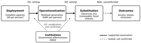
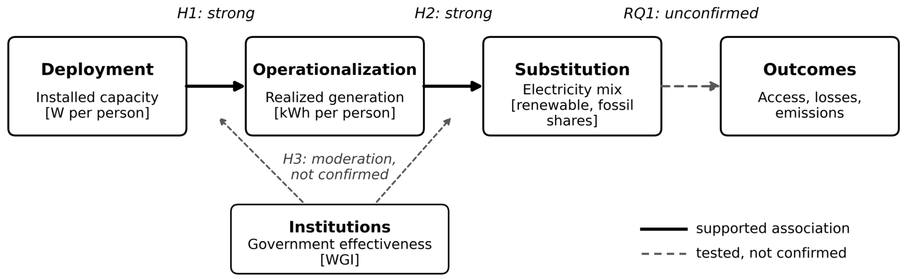
Figure 1 summarizes the framework. The chain runs from deployment through operationalization and substitution to broader outcomes; institutions are positioned as a potential moderator of the early links, and the evidence developed in Section 5 supports the first two links while leaving the third unconfirmed.

Figure 1. Conceptual chain from renewable deployment to broader outcomes. Notes: Boxes denote the four stages: installed non-hydro renewable capacity, realized non-hydro generation, the renewable and fossil shares of electricity output, and broader electricity-system and environmental outcomes. Solid arrows mark associations supported by the estimates (H1, H2); dashed arrows mark relationships that are tested but not confirmed (institutional moderation under H3, and the broader outcomes under RQ1). Evidence labels summarize the within-country panel estimates reported in Section 5. Source: author’s elaboration.

3. Data and Variable Construction

3.1. Data Sources

Renewable capacity and generation come from the IRENA Renewable Energy Statistics database (International Renewable Energy Agency, 2026), using the agency’s separate definitions and reporting conventions for maximum net generating capacity in megawatts (MW) and realized generation in gigawatt-hours (GWh) (International Renewable Energy Agency, 2024). IRENA compiles capacity and generation from distinct reporting streams and publishes them as separate series, so the two focal variables are not mechanically derived from one another, although the agency notes that matching capacity and production values can be absent for some country-years. The raw files retain country or area, technology, grid connection, year, unit, and generation-status fields. The data are harmonized through an ISO 3166-1 alpha-3 (ISO3) country crosswalk, and aggregates are preserved in the raw archive but excluded from the country-level estimation panel.

Electricity-system outcomes and macroeconomic controls come from the World Development Indicators (WDI; World Bank, 2026a). The analysis uses access to electricity, renewable electricity output, fossil-fuel electricity output, transmission and distribution losses, population, constant-price gross domestic product (GDP) per capita, gross capital formation, trade, and urban population. The environmental outcome uses the updated WDI series EN.GHG.CO2.PC.CE.AR5, carbon dioxide emissions excluding land use, land-use change, and forestry per person, rather than the discontinued legacy code. Absolute fossil and total electricity generation, used to test whether the electricity-mix results reflect displacement in levels, come from Ember’s yearly electricity data (Ember, 2026), accessed through the Our World in Data energy compilation (Our World in Data, 2026), in terawatt-hours converted to kilowatt-hours per person with WDI population; Ember does not cover the Marshall Islands or Kosovo.

Governance variables come from the Worldwide Governance Indicators (World Bank, 2026b; Kaufmann et al., 2010). Government effectiveness is the prespecified moderator because it most directly captures the capacity of the public sector to formulate and implement policy. Regulatory quality, rule of law, control of corruption, political stability, and voice and accountability are retained for sensitivity analysis. WGI measures are perception-based composites with reported uncertainty and limited short-run movement; this measurement structure is considered when interpreting interaction estimates.

3.2. Main Variables

Non-hydro renewable capacity is the sum of solar, wind, bioenergy, geothermal, and marine capacity. Non-hydro renewable generation is constructed from the same five technology families. The exclusion of hydropower follows the paper’s emphasis on contemporary deployment and avoids allowing long-established hydro systems to dominate the relationship. Capacity is converted to watts per person and generation to kilowatt-hours per person. The preferred variables are the natural logarithms of one plus these per capita measures, preserving zero observations while reducing leverage from the right tail. Because a log(1 + x) coefficient depends on the units in which the underlying variable is measured when the sample contains many zeros (Chen & Roth, 2024), the per capita measures are held in fixed units throughout, watts and kilowatt-hours per person, the coefficient is interpreted as an elasticity only for countries with established deployment where log(1 + x) approximates the logarithm, a Poisson (PPML) specification that places the outcome in levels is reported as a transformation-free check on the outcome side (Santos Silva & Tenreyro, 2006; Correia et al., 2020), and Section 5.2 reports the coefficient on the intensive margin and the pure log–log elasticity among positive observations, which does not depend on units.

The preferred exposure is an exact one-year calendar lag of non-hydro capacity. Government effectiveness is lagged in the same way for the interaction model. Exact-year matching is used throughout: values are not carried forward across gaps and the missing WGI observation for 2001 is not interpolated. Consequently, 2002 observations requiring a 2001 governance lag do not enter the relevant estimation sample.

The control set contains log real GDP per capita, gross capital formation as a percentage of GDP, trade as a percentage of GDP, and urban population as a percentage of total population. These variables capture broad differences in income, investment, openness, and settlement patterns without exhausting the limited within-country variation. Outcome-specific models use complete cases within the established 118-country universe.

3.3. Sample Construction and Descriptive Coverage

The complete merged panel contains 5824 country-year rows for 224 countries and areas over 2000–2025. Restricting the data to economies currently classified by the World Bank as low, lower-middle, or upper-middle income leaves 3406 observations for 131 economies. Requiring renewable generation, exact lagged non-hydro capacity, exact lagged government effectiveness, and the four controls yields the headline sample of 2252 observations for 118 economies over 2001–2023. The median country contributes 22 observations, with an unbalanced range of three to 22 observations. Because government effectiveness is required only where it is used, the headline capacity–generation, interaction, and conversion-efficiency models impose the exact lagged-governance requirement, while the electricity-mix and other secondary-outcome models require only their own outcome, lagged capacity, lagged government effectiveness, and the four controls; the secondary samples are therefore not nested in the headline sample and can be slightly larger. Section 5.2 additionally reports the headline relationship on the largest capacity–generation sample that drops the governance requirement, to confirm that the result is not an artifact of governance-complete coverage.

Table 1 reports descriptive statistics for the headline sample and the secondary outcomes. The sample averages 48.87 kWh of non-hydro renewable generation per person and 17.56 watts of lagged non-hydro capacity per person. Their maxima, 1141.75 kWh and 558.30 watts per person, reveal substantial cross-country dispersion. Lagged government effectiveness averages −0.556. Coverage for secondary outcomes is narrower and outcome-specific, ranging from 1782 observations for losses to 2248 for access in the final regression samples.

Table 1. Descriptive statistics for the headline sample and secondary outcomes.

	N	Mean	SD	Min	Median	Max
Non-hydro renewable generation	2252	48.867	108.609	0.000	4.151	1141.748
Lagged non-hydro renewable capacity	2252	17.558	38.881	0.000	1.933	558.299
Log lagged non-hydro renewable capacity	2252	1.569	1.567	0.000	1.076	6.327
Lagged government effectiveness	2252	−0.556	0.583	−2.206	−0.572	1.114
Log real GDP per capita	2252	7.796	0.893	5.759	7.933	9.611
Gross capital formation	2252	24.498	9.733	−15.678	23.303	76.782
Trade openness	2252	74.902	36.149	0.000	69.586	347.720
Urban population	2252	50.524	19.656	11.901	50.576	92.195
Renewable electricity output	1953	36.355	32.659	0.000	27.015	100.000
Fossil electricity output	2115	59.751	33.878	0.000	66.844	100.000
Transmission and distribution losses	1780	17.273	10.941	2.416	14.842	89.728
Electricity access	2236	73.220	30.388	3.300	88.200	100.000
CO2 excluding LULUCF	2179	2.080	2.417	0.002	1.138	15.727

Notes: Sample period 2001–2023, 118 economies. Headline variables use 2252 observations unless the outcome is secondary and coverage is narrower. Units: non-hydro generation in kWh per person; non-hydro capacity in W per person (its log in log(1 + x) form); real GDP per capita in constant prices (natural log); gross capital formation and trade in percent of GDP; urban population and electricity access in percent of population; renewable and fossil electricity output in percent of total electricity output; transmission and distribution losses in percent of output; CO₂ in tonnes of CO₂ equivalent per person; government effectiveness is the WGI estimate. Secondary-outcome regression samples are documented in Section 5.6.

4. Empirical Strategy

4.1. Baseline Two-Way Fixed-Effects Model

The baseline specification relates renewable generation to lagged renewable capacity and time-varying controls: y_it = β c_(i,t−1) + δ g_(i,t−1) + γ′X_it + μ_i + τ_t + ε_it. Here y is log(1 + x) non-hydro renewable generation per person, c is log(1 + x) non-hydro renewable capacity per person, g is government effectiveness, X is the control vector, and μ and τ are country and year fixed effects. The coefficient β is the focal conditional association. Because a coefficient near one has a substantive interpretation, β is tested against both zero and one; the test against one asks whether within-country conversion is statistically distinguishable from proportional.

Country fixed effects remove time-invariant differences in geography, resource endowments, legal origin, and long-run electricity-system structure. Year fixed effects absorb common technology, financing, commodity-price, and global-policy shocks. Standard errors are clustered by country in the preferred presentation. Two-way country-year clustering and Driscoll–Kraay standard errors with a Bartlett lag of two are reported as alternative inference procedures (Driscoll & Kraay, 1998). All estimation was carried out in Python (version 3.13.16) using the pyfixest package (version 0.60.0) for the fixed-effects, Poisson, and wild cluster bootstrap estimates.

4.2. Institutional Interaction

Institutional moderation is evaluated by adding the interaction between lagged capacity and lagged government effectiveness. Capacity and governance are centered within the exact estimation sample, so the capacity coefficient represents the association at average governance. A positive interaction would support H3. Because multiple governance indicators, direct-efficiency measures, and moderator families are examined, isolated raw p-values are not treated as sufficient evidence.

4.3. Robustness and Multiplicity

Robustness tests vary the functional form, timing, sample treatment, and estimator of uncertainty. The analysis compares levels, log(1 + x), and inverse hyperbolic sine transformations; contemporaneous, one-year, and two-year capacity on an exact common timing sample; pooled p1/p99 winsorization; and exclusion of rows with pooled-tail warnings. Four additional specification challenges address concerns that the baseline design leaves open. First, aggregate GWh and MW are used with log population so a shared per capita denominator cannot mechanically generate the result. Second, country-specific linear trends absorb persistent national trajectories. Third, exact annual first differences are estimated with year effects, with country effects added as a conservative variant, and extended to distributed lags in the current and lagged capacity changes so that the timing of the response can be read directly. Fourth, lagged solar, wind, bioenergy, geothermal, and marine capacity shares are held constant, followed by matched technology-specific models. Separate technology estimates require at least 12 countries with positive within-country capacity variation; geothermal is therefore exploratory and marine is excluded. Income- and region-specific models follow the same minimum-cluster principle. A Poisson (PPML) specification with the same fixed effects provides a transformation-free check on the outcome side, and an intensive-margin comparison together with a pure log–log elasticity on positive observations addresses the dependence of log(1 + x) coefficients on the units of measurement. For subgroup models with few country clusters, statistical significance is confirmed with a wild cluster restricted bootstrap (Cameron et al., 2008), which is more reliable than the cluster-robust variance when clusters are few. The country-trend and exact first-difference specifications together address the concern that non-hydro capacity and generation are trending or nonstationary series: the former removes country-specific linear trends, and the latter estimates the relationship entirely in annual changes, so a common trend cannot generate it.

Families of related institutional, heterogeneity, and secondary-outcome tests are adjusted using the Benjamini–Hochberg false-discovery-rate (FDR) procedure (Benjamini & Hochberg, 1995) and the Holm family-wise-error procedure (Holm, 1979). The manuscript distinguishes raw significance from multiplicity-robust evidence. This is particularly important for institutional results, where a favorable raw p-value can coexist with a null family-level conclusion.

4.4. Dynamic and Endogeneity Diagnostics

A lagged dependent variable is added to assess persistence and to calculate a diagnostic long-run association. Dynamic fixed-effects estimates can be biased in short panels, so they are not automatically superior to the static model. First-difference, Anderson–Hsiao, and collapsed difference generalized method of moments (GMM) specifications are also estimated, with explicit attention to first-stage strength, instrument count, serial-correlation assumptions, and overidentification tests (Nickell, 1981; Anderson & Hsiao, 1982; Arellano & Bond, 1991; Roodman, 2009). Lead and reverse-direction models provide additional diagnostics.

Reverse causality is the most direct threat to a conversion reading of the capacity coefficient, and three channels are plausible: past generation performance may encourage further investment, so that generation feeds capacity with a delay; demand growth may drive capacity additions and generation together; and capacity and generation may be revised jointly as reporting improves. The design limits these channels without eliminating them. The exposure is capacity recorded at the end of year t − 1, which is predetermined relative to generation in year t, so within-year feedback from generation to the installed stock is excluded by construction. Feedback across years is examined directly: a reverse-direction dynamic equation tests whether lagged generation predicts subsequent capacity, and the lead specifications test whether future capacity levels or future capacity growth carry information about current generation once lagged capacity is included. These diagnostics are reported in Section 5.5. They do not substitute for an external source of variation, and the capacity coefficient is interpreted as a conditional within-country association throughout.

None of these exercises is treated as a valid natural experiment. Internal instruments are acceptable only if their strength and specification tests support the required moment conditions. Where diagnostics fail, the estimates are retained for transparency and excluded from causal interpretation.

5. Empirical Results

5.1. Baseline Capacity-to-Generation Relationship

The baseline results in Table 2 strongly support H1. In the level specification, one additional watt of lagged non-hydro capacity per person is associated with 2.180 additional kWh of non-hydro generation per person (SE = 0.200, p < 0.001). In the preferred log(1 + x) specification, the coefficient is 1.042 (SE = 0.029, p < 0.001), and it is statistically indistinguishable from proportional conversion: a Wald test cannot reject the null that the coefficient equals one (p = 0.148). The within-country association is therefore not only positive but close to one-for-one. The coefficient on total renewable generation is positive but smaller at 0.285 (SE = 0.071, p < 0.001), illustrating the analytical value of separating contemporary non-hydro deployment from legacy hydropower.

Table 2. Baseline two-way fixed-effects estimates.

Variable/Statistic	Non-Hydro Levels	Non-Hydro log	Total log	Non-Hydro log + GE
Lagged non-hydro capacity	2.180 *** (0.200)
Log lagged non-hydro capacity		1.042 *** (0.029)	0.285 *** (0.071)	1.077 *** (0.035)
Lagged government effectiveness	−2.830 (7.067)	0.181 ** (0.073)	0.058 (0.141)	0.166 ** (0.078)
Log capacity × government effectiveness				−0.086 ** (0.041)
Observations	2252	2252	2252	2252
Countries/clusters	118	118	118	118
Country fixed effects	Yes	Yes	Yes	Yes
Year fixed effects	Yes	Yes	Yes	Yes
R-squared beyond fixed effects	0.757	0.763	0.168	0.766

Notes: Dependent variable: non-hydro renewable generation per person in kilowatt-hours (column 1) and in log(1 + x) form (columns 2 and 4); column 3 uses total renewable generation and total renewable capacity per person, including hydropower, both in log(1 + x) form. Capacity is one-year-lagged and measured in the same units per person as the outcome. Ordinary least squares (OLS) with country and year fixed effects over 2001–2023; all columns include controls for log GDP per capita, gross capital formation, trade openness, and urban population, and column 4 centers capacity and governance at their sample means. Country-clustered standard errors (CR1, the small-sample-adjusted cluster-robust estimator) are in parentheses. ** p < 0.05, *** p < 0.01. Estimates are conditional associations.

The interaction specification does not support the expected institutional amplification. Its capacity coefficient at average governance is 1.077, while the capacity-by-government-effectiveness coefficient is −0.086 (SE = 0.041, raw p = 0.039). The sign is opposite to H3, and the coefficient is small relative to the near-unit main effect and rests on limited within-country governance variation; as Section 5.3 shows, it does not survive the family-level multiple-testing correction applied to the institutional tests, so it does not support a substantive negative-governance claim.

5.2. Inference, Timing, Transformations, and Influential Observations

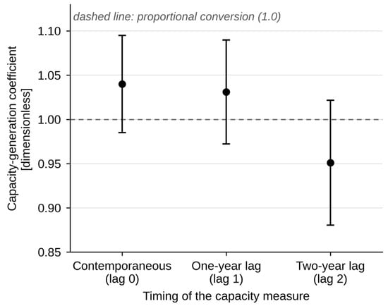
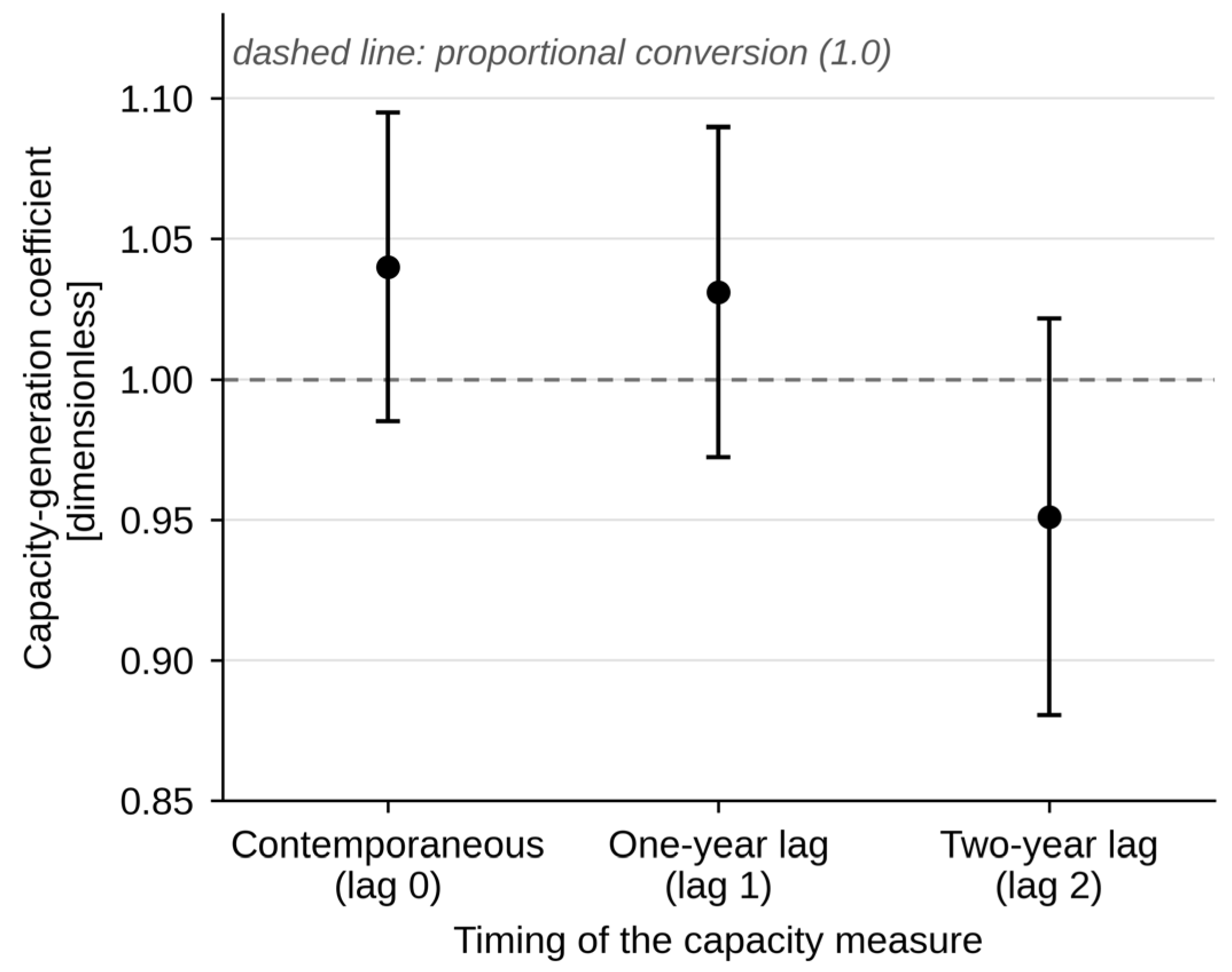
The preferred coefficient remains 1.042 under country clustering, two-way country-year clustering, and Driscoll–Kraay inference; the corresponding standard errors are 0.029, 0.027, and 0.018 (Table 3). On the exact timing sample, the contemporaneous, one-year, and two-year estimates are 1.040, 1.031, and 0.951, each within its confidence interval of proportional conversion (Figure 2). The result is therefore not driven by the selected one-year lag.

Table 3. Selected robustness estimates.

Specification	Coefficient	SE	p (β = 0)	Test of β = 1 (p)	N
log(1 + x), capacity association, C1	1.042	0.029	<0.001	0.148	2252
log(1 + x), capacity association, 2W	1.042	0.027	<0.001	–	2252
log(1 + x), capacity association, DK	1.042	0.018	<0.001	–	2252
Lag 0, capacity association	1.040	0.028	<0.001	–	2067
Lag 1, capacity association	1.031	0.030	<0.001	–	2067
Lag 2, capacity association	0.951	0.036	<0.001	–	2067
Inverse hyperbolic sine, capacity association	1.016	0.029	<0.001	–	2252
log(1 + x), capacity association, DROP	1.046	0.032	<0.001	–	2006
log(1 + x), capacity association, winsorized	1.049	0.029	<0.001	–	2252
Per capita logs + log population	1.043	0.031	<0.001	–	2252
Aggregate GWh/MW + log population	1.014	0.038	<0.001	0.717	2252
Country-specific linear trends	0.924	0.046	<0.001	0.097	2252
Exact first differences + year fixed effects	0.374	0.076	<0.001	<0.001	2045
Exact first differences + country and year fixed effects	0.308	0.082	<0.001	<0.001	2045
Distributed lag in levels, capacity at t, t − 1, t − 2: sum of lags	1.098	0.031	<0.001	0.002	2157
Distributed lag in exact first differences, changes at t, t − 1, t − 2: cumulative	1.070	0.044	<0.001	0.111	2034
Distributed lag in exact first differences, lagged changes t − 1 to t − 3: cumulative	0.509	0.076	<0.001	<0.001	2022
Lagged technology-share controls	1.025	0.029	<0.001	0.382	2252
Matched solar capacity–generation	1.036	0.021	<0.001	0.098	2252
Matched wind capacity–generation	1.135	0.041	<0.001	0.001	2252
Matched bioenergy capacity–generation	1.050	0.116	<0.001	0.669	2252
Matched wind, positive lagged wind capacity only	1.062	0.066	<0.001	0.356	1023
Poisson (PPML), levels outcome	0.923	0.060	<0.001	–	2195
log(1 + x), positive lagged capacity only (intensive margin)	1.004	0.034	<0.001	0.905	1904
Pure log–log, positive capacity and generation only	0.845	0.039	<0.001	<0.001	1892
log(1 + x), governance requirement dropped	1.048	0.028	<0.001	0.087	2352

Notes: Unless stated otherwise, models use the headline sample, the common controls, and country-clustered CR1 inference. The dependent variable is log(1 + x) non-hydro generation per person unless the row states otherwise (generation in levels for the Poisson row; matched technology-specific generation for the technology rows); all rows include country and year fixed effects unless stated; the sample period is 2001–2023; p-values are two-sided. The final column reports a Wald test of the null that the coefficient equals one (proportional conversion); it is shown for the distinct specifications for which proportionality is the relevant comparison and omitted (–) for the alternative-inference, timing, and outlier-robustness variants of the baseline estimate. First differences use exact annual changes over 2004–2023 (2045 observations). The Poisson (PPML) row places generation in levels and reports a semi-elasticity, for which proportionality is not a natural benchmark. The final row re-estimates the headline model on the largest capacity–generation sample after dropping the exact lagged-governance requirement. The technology-share model holds lagged solar, wind, bioenergy, geothermal, and marine shares constant. Solar, wind, and bioenergy have broad effective within-country coverage; geothermal is exploratory and marine is not estimated separately. The distributed-lag rows report the sum of the lag coefficients with a delta-method standard error; the levels version uses all headline rows with capacity at t, t − 1, and t − 2 (2157 observations), and the first-difference versions require exact consecutive changes, which is why their samples differ from the single-lag first-difference rows. The intensive-margin row keeps the log(1 + x) form on country-years with positive lagged capacity; the pure log–log row takes natural logarithms of positive capacity and generation only and is invariant to the units of measurement. The wind intensive-margin row restricts the matched wind model to the 74 economies with positive lagged wind capacity. C1, country-clustered CR1 standard errors; 2W, two-way country-year clustering; DK, Driscoll–Kraay standard errors; DROP, rows with pooled-tail warnings excluded.

Figure 2. Timing sensitivity of the capacity–generation association. Notes: Points show coefficient estimates on the exact common sample using contemporaneous, one-year-lagged, and two-year-lagged capacity; whiskers show 95 percent confidence intervals. The dashed horizontal line marks proportional conversion, a coefficient of one. Source: author’s calculations using IRENA, WDI, and WGI data.

Alternative transformations, measurement units, and outlier treatments produce similarly stable estimates. Proportional conversion is a benchmark defined for the log–log form; the level specification in Table 2 and the Poisson specification reported below confirm the sign, precision, and approximate magnitude of the relationship without testing a unit coefficient. The inverse hyperbolic sine coefficient is 1.016, the coefficient after pooled-tail exclusion is 1.046, and the p1/p99 winsorized coefficient is 1.049. This stability is much stronger than the institutional interaction, whose p-value changes from 0.039 under country clustering to 0.060 under two-way clustering and 0.005 under Driscoll–Kraay inference.

A log(1 + x) coefficient is also not invariant to the units of measurement when many observations are small (Chen & Roth, 2024), so the unit checks are stated explicitly. In the fixed units used here, watts and kilowatt-hours per person, 84.5 percent of headline observations have positive lagged capacity, and the coefficient on that intensive margin is 1.004 (SE = 0.034; test of unit coefficient, p = 0.905). Taking natural logarithms of positive capacity and generation only, which removes the dependence on units, gives a within-country elasticity of 0.845 (SE = 0.039), significantly below one (p < 0.001); the Poisson specification on the same observations gives 0.829 (SE = 0.046). Rescaling to kilowatts and megawatt-hours per person moves the log(1 + x) coefficient to 1.897 (SE = 0.159), because most observations then lie in the range where log(1 + x) behaves like a level and the slope reflects the ratio of kilowatt-hours to watts rather than an elasticity. The proportional benchmark is therefore not rejected in the fixed-unit log(1 + x) and Poisson forms and is rejected on the low side in pure logarithms among positive observations, which is consistent with mildly declining average utilization as national fleets grow. All forms agree that the association is large, precisely estimated, and close to proportional.

The four additional specification challenges point in the same direction. Adding log population to the per capita model gives 1.043 (SE = 0.031); using aggregate GWh and aggregate MW with log population gives 1.014 (SE = 0.038), a coefficient that cannot be distinguished from proportional conversion (test of unit coefficient, p = 0.717). Country-specific linear trends reduce the estimate to 0.924 (SE = 0.046) without eliminating it and without rejecting proportionality (p = 0.097). Exact annual first differences yield a markedly smaller 0.374 (SE = 0.076) with year effects and 0.308 (SE = 0.082) with country and year effects, over 2004–2023 (2045 observations); both differ significantly from one (p < 0.001). The contrast is informative rather than contradictory, and a distributed lag makes the timing explicit. Because the exposure is lagged capacity, the single first-difference coefficient relates this year’s change in generation to the previous year’s change in capacity. Entering the changes in capacity during the current, previous, and second-previous years jointly gives 0.711 (SE = 0.075), 0.279 (SE = 0.067), and 0.080 (SE = 0.034) with year effects, a cumulative response of 1.070 (SE = 0.044) that cannot be distinguished from one (p = 0.111) and is unchanged with country and year effects (1.070, SE = 0.056). The current-year change is not predetermined, so the cumulative response to predetermined changes, those of the previous three years, is reported alongside it: 0.509 (SE = 0.076). In levels, capacity at t, t − 1, and t − 2 entered jointly gives 0.735, 0.308, and 0.056, summing to 1.098 (SE = 0.031), slightly above one, and the dynamic model in Section 5.5 implies a long-run association of 1.009. The response to a capacity addition therefore arrives mainly within the year of installation and the year after, which is what commissioning dates, mid-year connection, and partial-year operation imply. The single-lag differenced coefficient should be read as one component of a short-run adjustment profile, not as a level elasticity comparable to the baseline.

Technology composition also does not explain the headline result. Controlling for lagged technology shares gives 1.025 (SE = 0.029), again indistinguishable from proportional (p = 0.382). Matched technology-specific coefficients are 1.036 for solar, 1.135 for wind, and 1.050 for bioenergy, all precisely estimated. Solar and bioenergy are statistically indistinguishable from one-for-one (p = 0.098 and p = 0.669), and the wind coefficient exceeds one (p = 0.001). The wind excess is an extensive-margin effect of the log(1 + x) transformation rather than a property of wind conversion: the matched model includes country-years with no wind capacity, and in the range where log(1 + x) approximates a level, the slope reflects the ratio of kilowatt-hours to watts, about two, rather than an elasticity. Among the 74 economies with positive lagged wind capacity (1023 observations) the coefficient is 1.062 (SE = 0.066; test of unit coefficient, p = 0.356), the pure log–log elasticity is 0.817 (SE = 0.099), and the Poisson coefficient is 0.846 (SE = 0.126). Fleet capacity factors have improved, from a median implied value of about 0.20 in 2001–2006 to about 0.28 in 2016–2023, but that improvement is a common trend absorbed by the year effects, not a within-country amplifier. Geothermal is positive and also exceeds one but is exploratory, resting on only 14 countries with useful within-country variation; marine is not estimated separately because only two countries meet that criterion.

Two further checks confirm that the result does not depend on the functional form or on the governance-complete sample. A Poisson specification that places generation in levels, avoiding the log(1 + x) transformation entirely, yields a coefficient of 0.92 on lagged log capacity per person (SE = 0.06, p < 0.001), close to the preferred estimate. Dropping the government-effectiveness requirement and re-estimating the headline model on the largest available capacity–generation sample, which adds 100 country-years across the same 118 economies, gives 1.048 (SE = 0.028) against the headline 1.042, so the relationship is not an artifact of governance-complete coverage. To make the magnitude concrete for established deployers, where the coefficient behaves as an elasticity, a doubling of lagged non-hydro capacity per person is associated with an approximately proportional, near-doubling increase in non-hydro generation per person.

5.3. Does Governance Moderate Conversion?

Direct conversion-efficiency tests, reported in Table 4, reinforce the institutional non-result. Government effectiveness has a coefficient of 0.104 (SE = 0.066, p = 0.116) in the model of log non-hydro generation per installed megawatt. In the standardized capacity–generation gap model, its coefficient is −0.058 (SE = 0.028, raw p = 0.039), but both the Benjamini–Hochberg and Holm adjusted p-values are 0.233. The winsorized average-capacity-factor proxy is also imprecisely related to government effectiveness.

Table 4. Institutional conversion and heterogeneity tests.

Test	Estimate	SE	Raw p	FDR-Adjusted p/Reading
Log non-hydro generation per installed MW: government effectiveness	0.104	0.066	0.116	0.606; does not survive FDR
Capacity–generation gap: government effectiveness	−0.058	0.028	0.039	0.233; does not survive FDR
Winsorized average-capacity-factor proxy: government effectiveness	3.700	2.753	0.182	No family adjustment
Capacity heterogeneity: initial hydropower-dominant renewable system	0.024	0.050	0.635	0.635; does not survive FDR
Capacity heterogeneity: low initial electricity access	−0.036	0.055	0.510	0.635; does not survive FDR
Capacity heterogeneity: low or lower-middle income	−0.033	0.049	0.499	0.635; does not survive FDR
Governance-moderation heterogeneity: low initial electricity access	0.187	0.089	0.037	0.056; does not survive FDR
Governance-moderation heterogeneity: low or lower-middle income	0.209	0.087	0.018	0.055; does not survive FDR

Notes: Family adjustments are calculated within prespecified groups of related tests. All rows are OLS with country and year fixed effects, the common controls, and country-clustered CR1 standard errors over 2001–2023; the first three rows use the dependent variables named in their labels, and the heterogeneity rows report interaction terms added to the headline log(1 + x) model. Raw p-values are two-sided. Raw significance is not treated as multiplicity-robust evidence.

The negative interaction is stable in sign and size across governance-timing, missing-data, and country-sample variants (Table A1). Interpolating the missing 2001 WGI value as the mean of 2000 and 2002, which restores 85 observations, gives −0.091 (SE = 0.041); contemporaneous governance gives −0.085 (SE = 0.042); a two-year lag gives −0.097 (SE = 0.040); leaving out each World Bank region in turn gives estimates between −0.075 and −0.129; and dropping China, India, and Brazil, states with fewer than one million people, economies with fewer than ten sample years, or the five largest per capita deployers gives estimates between −0.066 and −0.122, with raw p-values from 0.001 to 0.199. What is stable is also small. Lagged government effectiveness has a within-country standard deviation of 0.241 against a total standard deviation of 0.583, so only 17 percent of its variance is within countries, and a one-within-standard-deviation improvement changes the capacity slope by 0.021, under 2 percent of the slope at average governance (1.077). The design detects an interaction of about 0.115 with 80 percent power, so the null on amplification is not a power failure; the range over which governance moves within a country is too narrow for a moderator of this size to matter, and no variant supports the positive amplification of H3.

Capacity heterogeneity by initial hydropower dominance, low initial access, and lower-income status is null. Exploratory triple interactions for low-access and lower-income groups have raw p-values of 0.037 and 0.018, but their false-discovery-rate adjusted p-values are 0.056 and 0.055. They are suggestive enough to motivate future targeted work, but they do not establish a threshold or a general governance mechanism.

5.4. Income and Regional Patterns

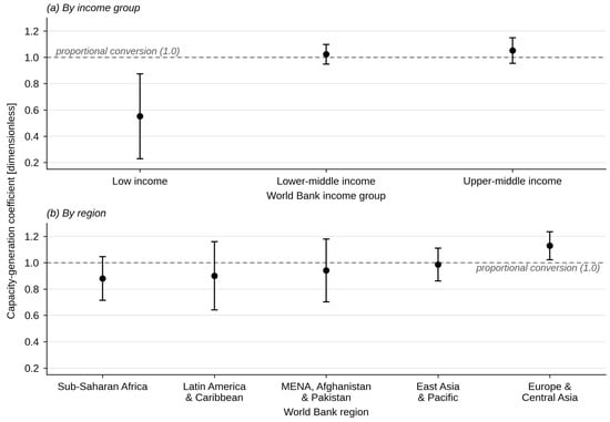
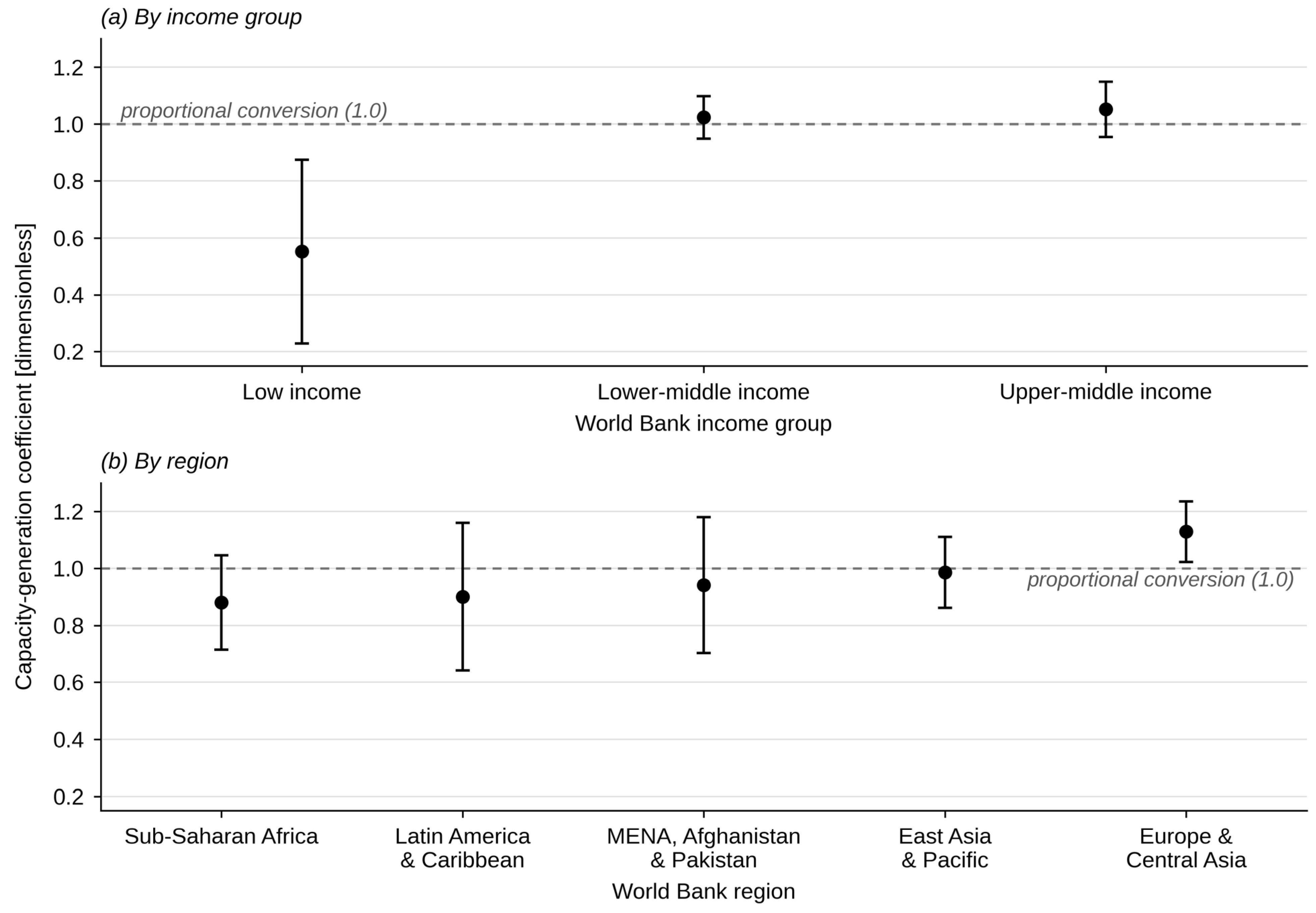
The capacity–generation association is positive within all three income groups and within each of the five regions, having at least 12 country clusters (Figure 3). Coefficients are 0.552 for low-income, 1.024 for lower-middle-income, and 1.052 for upper-middle-income economies. Regional estimates range from 0.880 in Sub-Saharan Africa to 1.129 in Europe and Central Asia. All eight subgroup coefficients survive family-level false-discovery-rate adjustment, and because several regions have as few as 14 country clusters, each regional coefficient is re-tested with a wild cluster restricted bootstrap; all remain significant, including the smallest group (p = 0.002). These stratified estimates support broad generality, but they do not constitute formal evidence that slopes are equal across groups. South Asia is not reported separately because it contains only six country clusters.

Figure 3. Capacity–generation estimates across income groups and regions. Notes: Panel (a) reports estimates by income group and panel (b) by region. Points show subgroup coefficient estimates and whiskers show 95 percent confidence intervals, and the dashed horizontal line marks proportional conversion, a coefficient of one. Subgroup models include country and year fixed effects. Region-specific estimates require at least 12 country clusters; South Asia is excluded from separate reporting. Source: author’s calculations using IRENA, WDI, and WGI data.

5.5. Persistence and Internal-Instrument Diagnostics

Generation is highly persistent (Table 5). In the dynamic non-hydro log model, the lagged dependent-variable coefficient is 0.704 and the short-run capacity coefficient is 0.298 (SE = 0.047, p < 0.001). The implied long-run association is 1.009 (SE = 0.058), close to the static coefficient. The static result is therefore not eliminated when persistence is modeled.

Table 5. Dynamic and endogeneity diagnostics.

Model	Estimate	p-Value	Diagnostic	Interpretation
Dynamic two-way fixed effects: non-hydro log	0.298	<0.001	Persistence diagnostic; long-run association stable	Robustness/persistence
Anderson–Hsiao: instrument lagged outcome	−1.307	0.012	Unstable persistence and weak excluded instrument	Diagnostic only
Anderson–Hsiao: instrument outcome and capacity	0.486	0.762	Weak first stages; not credible for causal identification	Diagnostic only
Difference GMM: collapsed lags 2–3	−0.254	0.216	Hansen rejection; invalid as headline evidence	Diagnostic only
Future-capacity lead diagnostic	0.368	<0.001	Future level significant; persistence/anticipation warning	Diagnostic only
Future-capacity-growth diagnostic	0.028	0.556	Future capacity growth not significant	Diagnostic only
Reverse-direction dynamic capacity equation	0.001	0.975	No evidence that generation predicts later capacity in this diagnostic	Diagnostic only

Notes: Internal-instrument rows are shown for transparency but are not used to support causal claims. All rows use the headline sample (2001–2023) with the common controls and country-clustered inference; fixed-effects rows include country and year effects, and the Anderson–Hsiao and difference-GMM rows are estimated in first differences. Section 5.5 states which coefficient each row reports. Full first-stage and specification diagnostics are available in the reproducibility archive.

The instrument-based exercises do not identify a credible causal effect. Anderson–Hsiao specifications have weak first stages and, in some cases, implausible persistence estimates. The collapsed lag-2 difference-GMM model is exactly identified and weak, while the lag-2/3 model rejects the overidentifying restrictions (Hansen p = 0.0004). A future capacity level is significant, whereas future capacity growth is not; the level result is consistent with the persistence of installed stocks and is retained as a warning rather than resolved, while the insignificant growth term indicates that current generation does not anticipate subsequent capacity changes. The reverse-direction dynamic equation addresses feedback across years directly: lagged generation does not predict later capacity (coefficient 0.001, p = 0.975), so this design provides no evidence that realized generation drives subsequent deployment. Taken together, these diagnostics support the transparent fixed-effects model as the headline associational specification and rule out causal language.

5.6. Electricity-Mix and Broader Outcomes

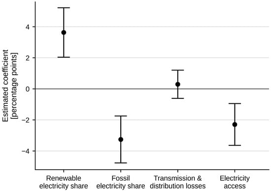
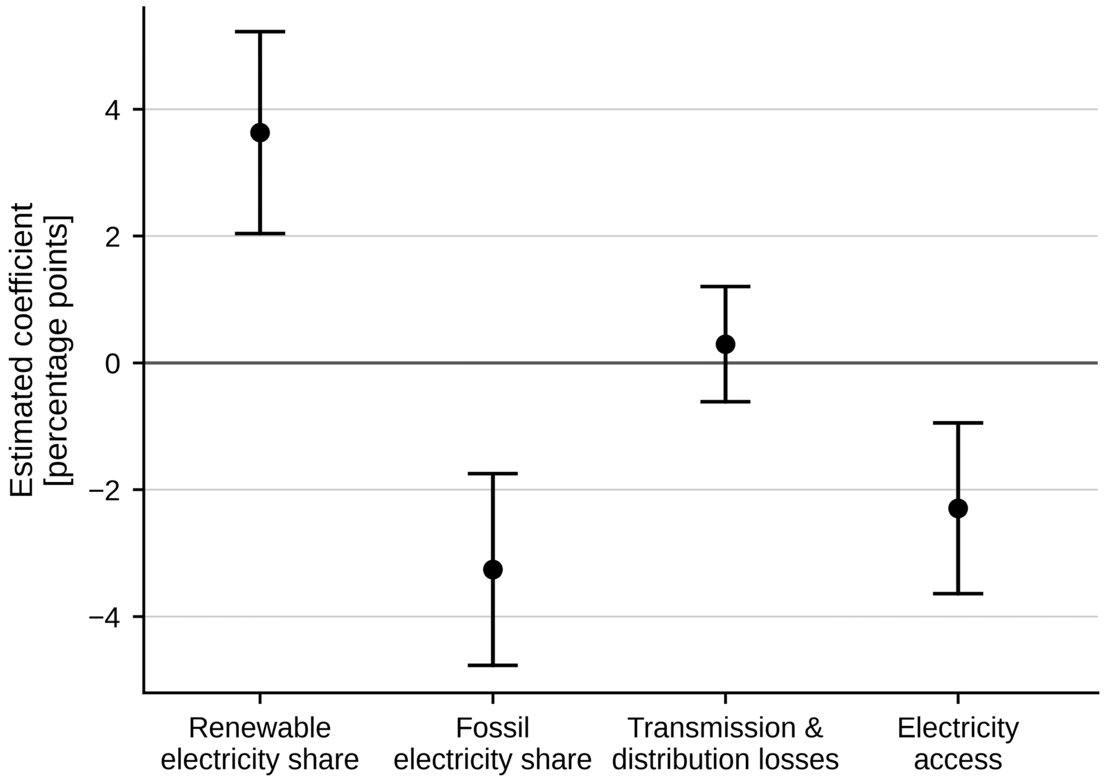
The electricity-mix results in Table 6 support H2. A one-unit increase in lagged log(1 + x) non-hydro capacity is associated with a 3.630 percentage-point increase in renewable electricity output share (SE = 0.813) and a 3.258 percentage-point decline in fossil electricity output share (SE = 0.771; Figure 4). Both results survive country clustering, two-way clustering, Driscoll–Kraay inference, Benjamini–Hochberg adjustment, and Holm adjustment. To fix the scale, a one-unit change in the exposure near the sample median corresponds to raising lagged non-hydro capacity from roughly 2 to 7 watts per person, so a move of that size is associated with about 3.6 percentage points more renewable and 3.3 percentage points less fossil electricity. Because these outcomes measure the composition of electricity supply rather than its volume, they are evidence that deployment is accompanied by system-level substitution and not merely additional renewable output.

Table 6. Secondary electricity-system outcomes.

Outcome	Estimate	SE	Raw p	FDR p	N	Reading
Renewable electricity output (percent)	3.630	0.813	<0.001	<0.001	1965	Robust positive mix association
Fossil-fuel electricity output (percent)	−3.258	0.771	<0.001	<0.001	2127	Robust negative fossil-share association
Electric power transmission and distribution losses (percent)	0.294	0.463	0.528	0.660	1782	No reliable association
Access to electricity (percent of population)	−2.295	0.686	0.001	0.002	2248	Ceiling effect; see access rows below
Log CO2 emissions per capita (log(1 + tCO2e/person))	−0.004	0.013	0.792	0.792	2191	No reliable association
Fossil generation per person, log(1 + kWh)	−0.105	0.056	0.061	0.100	2229	Modest absolute displacement
Total generation per person, log(1 + kWh)	−0.043	0.026	0.100	0.100	2229	No expansion association
Fossil generation per person, Poisson	−0.065	0.025	0.012	0.024	2190	Modest absolute displacement
Total generation per person, Poisson	−0.018	0.023	0.444	0.444	2229	No expansion association
Access, country-years at or above 99 percent dropped	0.107	0.854	0.900	–	1572	Ceiling removed; no association
Access, country-years at 100 percent dropped	−0.571	0.733	0.438	–	1970	Ceiling removed; no association
Access, logit of the access share	−0.060	0.063	0.346	–	2248	Bounded outcome; no association

Notes: Renewable share, fossil share, losses, and access are percentage-point outcomes. Estimates are OLS coefficients on one-year-lagged log(1 + x) non-hydro capacity per person from models with country and year fixed effects, lagged government effectiveness, and the common controls, over 2001–2023 on outcome-specific complete cases, with country-clustered CR1 standard errors; raw p-values are two-sided and FDR-adjusted p-values are Benjamini–Hochberg within the secondary-outcome family. CO₂ is log(1 + tCO₂e per person) and is not directly comparable with percentage-point coefficients. All estimates are conditional associations. Fossil and total generation per person are from Ember’s yearly electricity data, which do not cover the Marshall Islands and Kosovo, converted to kilowatt-hours per person with WDI population; their FDR adjustment is within the fossil-total pair for each estimator, and the Poisson rows report semi-elasticities. The Poisson fossil model excludes Bhutan and Lesotho, which report no fossil generation in any sample year. The access ceiling rows use the same specification and sample as the access row; the FDR column does not apply to these robustness rows.

Figure 4. Secondary electricity-system outcomes. Notes: Points show coefficient estimates in percentage points and whiskers show 95 percent confidence intervals; the solid horizontal line marks zero. CO₂ is omitted because its coefficient is on a different log scale. The negative access estimate is a ceiling effect of near-universal access in many country-years (Section 5.6) and must not be interpreted causally. Source: author’s calculations using IRENA, WDI, and WGI data.

Whether the compositional shift reflects absolute displacement or faster growth of total supply is tested directly with generation levels from Ember, which cover 116 of the 118 economies. With the same specification as the share models, a one-unit increase in lagged log(1 + x) non-hydro capacity is associated with a change of −0.105 in log(1 + x) fossil generation per person (SE = 0.056, p = 0.061) and of −0.043 in log(1 + x) total generation per person (SE = 0.026, p = 0.100); the Poisson specifications give −0.065 for fossil generation (SE = 0.025, p = 0.012) and −0.018 for total generation (SE = 0.023, p = 0.444). Total supply per person is therefore not systematically higher where non-hydro capacity is higher, and fossil generation per person is modestly lower, so the falling fossil share reflects displacement at the margin rather than expansion of the system around unchanged fossil output. The level evidence is less precise than the share evidence, and the fossil coefficient in log(1 + x) form is significant only at the 10 percent level, so the absolute displacement is characterized as modest.

The broader outcomes, addressed as RQ1, do not show consistent gains. Transmission and distribution losses have a small, imprecise coefficient of 0.294 (p = 0.528). Log per capita carbon emissions have a coefficient of −0.004 (p = 0.792) using the updated WDI series. Electricity access has a negative coefficient of −2.295 percentage points in the full sample (SE = 0.686; FDR-adjusted p = 0.002), and the access interaction with government effectiveness is also negative. This is a ceiling effect rather than a substantive association. Access stands at 100 percent in 12.4 percent of the sample country-years and at or above 99 percent in 29.9 percent of them, and 19 of the 117 economies with access data were already at or above 99 percent in their first sample year; in those observations access cannot rise while capacity does. Dropping country-years at or above 99 percent gives 0.107 (SE = 0.854, p = 0.900), dropping only those at 100 percent gives −0.571 (SE = 0.733, p = 0.438), and modeling the logit of the access share, which respects the bound, gives −0.060 (SE = 0.063, p = 0.346). Dropping instead the 19 economies that began the sample at or above 99 percent leaves −1.913 (SE = 0.917, p = 0.040), while dropping every economy that reaches 100 percent at any point gives 1.087 (SE = 1.126, p = 0.338), so the saturation that produces the negative coefficient occurs during the sample rather than only at its start. The full-sample coefficient must therefore not be read as evidence that renewable deployment reduces access; it reflects a bounded outcome.

6. Discussion

6.1. What the Robust Conversion Result Means

The central finding is narrower than a claim that renewable deployment automatically produces sustainable development, but it is also more defensible. Installed non-hydro capacity is closely connected to operational non-hydro generation across a wide group of developing and emerging economies, and the connection is close to one-for-one: the headline coefficient, the aggregate-unit specification, and the technology-share specification are all statistically indistinguishable from proportional conversion, while the pure log–log elasticity among positive observations, 0.845, is below one, so the relationship is best described as close to proportional rather than exactly so. The relationship is not an artifact of common per capita scaling, since aggregate GWh on aggregate MW with log population yields 1.014, and it is not an artifact of a shared trend, since it remains 0.924 with country-specific trends and stays significantly positive in exact annual first differences. The single-lag first-difference magnitude is smaller because it captures only the response to the previous year’s capacity change; the distributed lag shows that the response arrives mainly within the year of installation and the year after and cumulates to 1.070, so the near-proportional long-run relationship is what remains once commissioning lags resolve. The relationship also appears in the electricity mix, where renewable output shares rise and fossil output shares fall by comparable and multiplicity-robust amounts. This last result is the strongest evidence that deployment corresponds to system-level substitution rather than merely to additional renewable output, and the generation levels point the same way: total generation per person is not higher where non-hydro capacity is higher, while fossil generation per person is modestly lower.

This evidence validates capacity as a meaningful indicator of transition effort while showing why it should not be used alone. Matched coefficients are 1.036 for solar, 1.135 for wind, and 1.050 for bioenergy, and the wind excess above one disappears on the intensive margin (1.062), indicating that the aggregate result is not confined to one technology and that the treatment of entry from zero under log(1 + x), not a wind-specific property, produces the excess. The geothermal estimate is positive but rests on only 14 countries with useful within-country variation, and marine cannot support separate inference. Monitoring frameworks should pair watts per person with generation per person, technology composition, and electricity-mix measures. Capacity records commitment and infrastructure; generation and composition reveal whether that infrastructure operates within the system.

6.2. Why the Institutional Hypothesis Is Not Confirmed

The institutional non-result does not imply that governance is irrelevant to renewable energy. Recent evidence links institutions to renewable capital flows and development, although signs and nonlinearities vary (Pan et al., 2023; Dube & Horvey, 2023). The result here is downstream and narrower: annual, broad WGI measures do not robustly explain the marginal conversion of already-installed non-hydro capacity into generation in this sample and design. Governance may exert its strongest influence earlier, through project selection, finance, procurement, permitting, or grid investment, or through sector-specific capabilities that broad national indicators cannot measure.

Measurement and variation also matter. WGI estimates are perception-based composites with uncertainty, and within-country variation is limited: only 17 percent of the variance in lagged government effectiveness is within countries, and a change of one within-country standard deviation in governance moves the capacity slope by about 0.02. The interaction is therefore not underpowered so much as economically small over the range governance actually moves within a country, and interaction coefficients remain sensitive to measurement error within that narrow range. Future work should therefore combine national governance with power-sector regulatory indicators, project commissioning data, curtailment, grid-connection delays, transmission investment, and utility performance. Such data would test the mechanism more directly than a broad governance score.

6.3. Interpreting the Access Result

The negative access association is a ceiling effect. Access is bounded at 100 percent; nearly a third of the sample country-years sit at or above 99 percent, and in those observations, access cannot rise while capacity continues to grow, which produces a negative within-country slope mechanically. Once country-years at or near the ceiling are removed, or the bounded outcome is modeled on the logit scale, the association is small, imprecise, and of indeterminate sign (Section 5.6). The substantive reading is therefore not that deployment lowers access but that the panel does not identify any access effect of utility-scale non-hydro deployment. Rollout sequencing, the distinction between utility-scale transition and last-mile electrification, and residual time-varying confounding remain relevant to the unsaturated observations, and because the model is not designed around an access intervention, no welfare claim is made in either direction.

6.4. Policy Implications

The results suggest three practical priorities. First, governments and international organizations should publish capacity and generation together at consistent technology detail. Second, renewable deployment targets should be accompanied by operational indicators covering generation, curtailment, outages, connection delays, flexibility, and electricity-mix substitution; these correspond to the grid and implementation constraints highlighted in current international assessments (International Energy Agency, 2024). Third, access policy should not assume that utility-scale renewable expansion will automatically solve last-mile electrification; grid extension, mini-grids, affordability, and service quality require separate design and evaluation.

The study does not justify a universal governance threshold or a numerical institutional prerequisite for successful conversion. Policy recommendations should therefore avoid treating a broad governance score as a switch that determines whether renewable projects work. More specific administrative and power-sector capabilities are better targets for diagnosis and reform.

6.5. Limitations and Future Research

The analysis has several main limitations. It is observational and lacks an external source of plausibly exogenous variation in deployment. Country-year aggregates mask project and within-country heterogeneity, and the pooled two-way fixed-effects slope averages over country-specific institutional, regulatory, and market arrangements, including tariff design, procurement rules, grid-connection practice, and utility ownership; the subgroup estimates in Section 5.4 describe part of that heterogeneity but do not exhaust it. End-of-year capacity and annual generation are not perfectly aligned in time, because an asset commissioned during a year is counted in full in year-end capacity but contributes only part of a year of generation. Broad governance measures may miss sector-specific capabilities and contain measurement error. Technology-specific evidence is uneven, making geothermal estimates exploratory and preventing separate marine estimation. Because hydropower is excluded by design, the estimates characterize non-hydro deployment and need not transfer to systems in which hydropower dominates renewable supply; the total-renewables coefficient in Table 2 shows how differently pooled legacy hydro behaves, and the hydro-dominance interaction in Table 4 indicates only that the non-hydro slope itself does not differ in initially hydro-dominant systems. Outcome coverage differs across WDI series, so downstream models are not estimated on an identical sample, and complete-case estimation means that countries missing an outcome or control in a given year are dropped, which could introduce selection if missingness is related to the outcomes; the stability of the headline coefficient when the governance requirement is dropped and the sample expands is reassuring on this point but does not eliminate the concern.

Future research can improve identification by exploiting policy discontinuities, auctions, financing shocks, connection queues, or project-level commissioning schedules. It can also test whether transmission expansion, storage, curtailment rules, or utility governance mediate conversion. A formal panel-threshold or quantile model should be treated as a separately estimated extension; the current linear interactions do not establish a threshold, and the mean-regression estimates describe the conditional average conversion rate rather than its behavior across the conditional distribution of generation, the question that quantile approaches address (Ul-Durar et al., 2026).

7. Conclusions

This paper asks what lies beyond installed renewable capacity. Across 118 developing and emerging economies from 2001 to 2023, greater non-hydro renewable capacity is consistently associated with greater non-hydro renewable generation, at a rate close to one-for-one: the fixed-unit log(1 + x) and Poisson specifications cannot reject proportional conversion, the pure log–log elasticity among positive observations is 0.845, and the estimate is stable across alternative inference, timing, outlier treatments, a common-denominator challenge, country-specific trends, and technology-composition controls. Matched results for solar and bioenergy are similarly near-proportional, as is wind on the intensive margin, so the headline relationship is not confined to one technology. A distributed lag in exact first differences shows that the response to a capacity addition arrives mainly within the year of installation and the year after, as commissioning and partial-year operation imply. Capacity expansion is also associated with a larger renewable electricity share, a smaller fossil electricity share, and modestly lower fossil generation per person with no rise in total generation per person, the clearest sign that deployment corresponds to a changing electricity mix and not only to additional output.

The evidence does not support the stronger claim that government effectiveness or other broad governance indicators systematically amplify this conversion. That absence does not mean governance is irrelevant to renewable deployment; it means that broad, annual WGI measures do not explain the marginal conversion of already-installed non-hydro capacity into generation in this sample and design. Nor do the models establish gains in electricity access, transmission efficiency, or per capita carbon emissions. Internal-instrument diagnostics are too weak or invalid to support causal interpretation.

The resulting contribution is an evidence hierarchy rather than a universal development claim. Capacity is an important but incomplete measure of energy transition. Its strongest observable counterpart is operational generation and a changing electricity mix. For applied panel practice, the exercise also illustrates the value of testing a substantive coefficient benchmark rather than reporting sign and significance alone, of pairing log(1 + x) estimates with an intensive-margin elasticity and a transformation-free Poisson check when zeros are present, and of matching inference to the cluster structure that subgroup models actually leave available. For measurement, policy, and future research, the lesson is straightforward: count megawatts, but also verify what they produce and what they replace.

References

- Aguirre, M., & Ibikunle, G. (2014). Determinants of renewable energy growth: A global sample analysis. Energy Policy, 69, 374–384. [Google Scholar] [CrossRef] [Scilit]
- Anderson, T. W., & Hsiao, C. (1982). Formulation and estimation of dynamic models using panel data. Journal of Econometrics, 18(1), 47–82. [Google Scholar] [CrossRef] [Scilit]
- Arellano, M., & Bond, S. (1991). Some tests of specification for panel data: Monte Carlo evidence and an application to employment equations. Review of Economic Studies, 58(2), 277–297. [Google Scholar] [CrossRef] [Scilit]
- Benjamini, Y., & Hochberg, Y. (1995). Controlling the false discovery rate: A practical and powerful approach to multiple testing. Journal of the Royal Statistical Society Series B, 57(1), 289–300. [Google Scholar] [CrossRef] [Scilit]
- Bolson, N., Prieto, P., & Patzek, T. (2022). Capacity factors for electrical power generation from renewable and nonrenewable sources. Proceedings of the National Academy of Sciences, 119(52), e2205429119. [Google Scholar] [CrossRef] [Scilit]
- Cadoret, I., & Padovano, F. (2016). The political drivers of renewable energies policies. Energy Economics, 56, 261–269. [Google Scholar] [CrossRef] [Scilit]
- Cameron, A. C., Gelbach, J. B., & Miller, D. L. (2008). Bootstrap-based improvements for inference with clustered errors. Review of Economics and Statistics, 90(3), 414–427. [Google Scholar] [CrossRef] [Scilit]
- Chen, J., & Roth, J. (2024). Logs with zeros? Some problems and solutions. The Quarterly Journal of Economics, 139(2), 891–936. [Google Scholar] [CrossRef] [Scilit]
- Correia, S., Guimarães, P., & Zylkin, T. (2020). Fast Poisson estimation with high-dimensional fixed effects. The Stata Journal, 20(1), 95–115. [Google Scholar] [CrossRef] [Scilit]
- Driscoll, J. C., & Kraay, A. C. (1998). Consistent covariance matrix estimation with spatially dependent panel data. Review of Economics and Statistics, 80(4), 549–560. [Google Scholar] [CrossRef] [Scilit]
- Dube, A., & Horvey, S. S. (2023). Institutional quality and renewable energy capital flows in Africa. Future Business Journal, 9(1), 55. [Google Scholar] [CrossRef] [Scilit]
- Ember. (2026). Yearly electricity data. Ember. Available online: https://ember-energy.org/data/yearly-electricity-data/ (accessed on 7 August 2026).
- Holm, S. (1979). A simple sequentially rejective multiple test procedure. Scandinavian Journal of Statistics, 6(2), 65–70. [Google Scholar]
- International Energy Agency. (2024). Renewables 2024. IEA. Available online: https://www.iea.org/reports/renewables-2024 (accessed on 7 August 2026).
- International Renewable Energy Agency. (2024). Renewable energy statistics 2024. IRENA. Available online: https://www.irena.org/Publications/2024/Jul/Renewable-energy-statistics-2024 (accessed on 7 August 2026).
- International Renewable Energy Agency. (2026). IRENA renewable energy statistics database and statistical notes. IRENASTAT. Available online: https://www.irena.org/Data/Statistical-publications/Notes-and-Methodology (accessed on 7 August 2026).
- Karlilar Pata, S., & Balcilar, M. (2024). Decarbonizing energy: Evaluating fossil fuel displacement by renewables in OECD countries. Environmental Science and Pollution Research, 31(21), 31304–31313. [Google Scholar] [CrossRef] [Scilit]
- Kaufmann, D., Kraay, A., & Mastruzzi, M. (2010). The Worldwide Governance Indicators: Methodology and analytical issues (Policy Research Working Paper 5430). World Bank. [Google Scholar] [CrossRef] [Scilit]
- Kwakwa, P. A. (2023). Climate change mitigation role of renewable energy consumption: Does institutional quality matter in the case of reducing Africa’s carbon dioxide emissions? Journal of Environmental Management, 342, 118234. [Google Scholar] [CrossRef] [Scilit]
- Li, W., Ji, Z., & Dong, F. (2022). Global renewable energy power generation efficiency evaluation and influencing factors analysis. Sustainable Production and Consumption, 33, 438–453. [Google Scholar] [CrossRef] [Scilit]
- Liddle, B. (2024). To what extent do alternative energy sources displace coal and oil in electricity generation? A mean-group panel analysis. Sustainability, 16(13), 5319. [Google Scholar] [CrossRef] [Scilit]
- Marques, A. C., Fuinhas, J. A., & Pires Manso, J. R. (2010). Motivations driving renewable energy in European countries: A panel data approach. Energy Policy, 38(11), 6877–6885. [Google Scholar] [CrossRef] [Scilit]
- Nickell, S. (1981). Biases in dynamic models with fixed effects. Econometrica, 49(6), 1417–1426. [Google Scholar] [CrossRef] [Scilit]
- Our World in Data. (2026). Data on energy by Our World in Data. Our World in Data. Available online: https://github.com/owid/energy-data (accessed on 7 August 2026).
- Pan, X., Dossou, T. A. M., Berhe, M. W., & Kambaye, E. N. (2023). Towards efforts to promote renewable energy development in Africa: Does governance quality matter? Energy & Environment, 34(8), 3039–3054. [Google Scholar] [CrossRef] [Scilit]
- Pfeiffer, B., & Mulder, P. (2013). Explaining the diffusion of renewable energy technology in developing countries. Energy Economics, 40, 285–296. [Google Scholar] [CrossRef] [Scilit]
- Polzin, F., Migendt, M., Täube, F. A., & von Flotow, P. (2015). Public policy influence on renewable energy investments—A panel data study across OECD countries. Energy Policy, 80, 98–111. [Google Scholar] [CrossRef] [Scilit]
- Rahman, M. M., & Sultana, N. (2022). Impacts of institutional quality, economic growth, and exports on renewable energy: Emerging countries perspective. Renewable Energy, 189, 938–951. [Google Scholar] [CrossRef] [Scilit]
- Romano, A. A., Scandurra, G., Carfora, A., & Fodor, M. (2017). Renewable investments: The impact of green policies in developing and developed countries. Renewable and Sustainable Energy Reviews, 68, 738–747. [Google Scholar] [CrossRef] [Scilit]
- Roodman, D. (2009). How to do xtabond2: An introduction to difference and system GMM in Stata. The Stata Journal, 9(1), 86–136. [Google Scholar] [CrossRef] [Scilit]
- Santos Silva, J. M. C., & Tenreyro, S. (2006). The log of gravity. Review of Economics and Statistics, 88(4), 641–658. [Google Scholar] [CrossRef] [Scilit]
- Ul-Durar, S., Dimitriadis, K. A., Arshed, N., De Sisto, M., & Harati, H. (2026). Distributional and tail-dependent perspectives in economic relationships: A review of quantile regression application. Journal of Economic Surveys, 40(3), 1637–1652. [Google Scholar] [CrossRef] [Scilit]
- United Nations Statistics Division. (2024). Metadata for SDG indicator 7.b.1: Installed renewable energy-generating capacity in developing and developed countries (in watts per capita). United Nations. Available online: https://unstats.un.org/sdgs/metadata/files/Metadata-07-0b-01.pdf (accessed on 7 August 2026).
- Uzar, U. (2020). Political economy of renewable energy: Does institutional quality make a difference in renewable energy consumption? Renewable Energy, 155, 591–603. [Google Scholar] [CrossRef] [Scilit]
- World Bank. (2026a). World Development Indicators. World Bank. Available online: https://data.worldbank.org/ (accessed on 7 August 2026).
- World Bank. (2026b). Worldwide Governance Indicators: Documentation. World Bank. Available online: https://www.worldbank.org/en/publication/worldwide-governance-indicators/documentation (accessed on 7 August 2026).
- York, R. (2012). Do alternative energy sources displace fossil fuels? Nature Climate Change, 2(6), 441–443. [Google Scholar] [CrossRef] [Scilit]
Disclaimer/Publisher’s Note: The statements, opinions and data contained in all publications are solely those of the individual author(s) and contributor(s) and not of MDPI and/or the editor(s). MDPI and/or the editor(s) disclaim responsibility for any injury to people or property resulting from any ideas, methods, instructions or products referred to in the content. |
© 2026 by the author. Licensee MDPI, Basel, Switzerland. This article is an open access article distributed under the terms and conditions of the Creative Commons Attribution (CC BY) license.