


Abstract
Advances in large language models (LLMs) have accelerated the real-world deployment of embodied intelligent robots, supporting intuitive human–robot interaction without specialized robotics expertise. However, few systematic assessments examine how well LLMs translate natural-language route instructions into executable robot command sequences, particularly for non-English instructions and across deployment-relevant model classes. In this paper, a Chinese route-instruction corpus was constructed, which comprised 212 instructions collected from six native speakers across 50 procedurally generated town maps. Each was annotated with a ground-truth command sequence verified by simulation to reach its goal, and a 100% performance ceiling was established. Using this corpus, 12 LLMs spanning three capability tiers—cloud proprietary models, mid-sized open-weight models, and small open-weight models—were evaluated under three system prompts differing only in the number of worked examples (zero, one, and three). Open-weight models in the 3–9B range reached at most 9.2% of goals, while proprietary cloud models reached 80.0%, a substantial gap that increasing the number of worked examples did not measurably narrow. A paired analysis across the three prompt conditions detected no reliable effect of demonstration count: pooled path_reach rose modestly from 25.0% under zero-shot prompting to 27.2% with one example and 27.7% with three examples (three versus zero examples: odds ratio: 1.15; 95% CI: 0.98–1.34). None of these differences was significant after multiple-comparison correction (Holm-adjusted p ≥ 0.247). Low-Rank Adaptation (LoRA) fine-tuning on 126 examples raised mid-sized open-weight models to 27.7–35.4%, and the gain spanned both output-format compliance and route competence.
1. Introduction
As robots are deployed in ordinary settings, their operators are typically non-specialists in robotics. When a passenger directs an autonomous vehicle “turn there” or “go right at the end of the road,” they rely on the same egocentric, informal language used in human communication. If robots are to be usable outside the laboratory, they must accept instructions of this kind. Whether a large language model (LLM) can convert such an utterance into an executable command sequence remains an open deployment question. Deruyttere et al. [1] built the Talk2Car dataset exactly on this premise, collecting free-form natural-language commands that a passenger might issue to a self-driving car and grounding each to an object in the scene. Sriram et al. [2] addressed the navigational counterpart, mapping natural-language encodings to local waypoints, so that a vehicle could follow an instruction to turn at a particular point without a map registered in advance. In both cases, the defining property of the input was: it was produced by someone not thinking about the robot’s internal representation. However, these instructions are hard to execute. First, “a little further” and “just past the door” carry no metric value. Second, each clause is interpreted relative to the robot’s pose after the previous clause has been executed, so a single misparse propagates through the remainder of the route. Third, landmarks named in the instruction must correspond to something the robot can perceive.
Therefore, LLMs have been extensively investigated to address this problem. Capable of parsing unconstrained natural language and generating structured outputs without task-specific training, they can serve as the language front-end of a navigation stack [3,4,5]. This raises a practical question: To what extent does task performance depend on model selection versus prompt formulation? The two classes available in practice differ sharply: open-weight models of a few billion parameters are the class that could in principle be self-hosted, whereas cloud models are the class with the highest capability. The present study compared these model classes under identical instructions and prompts. It did not evaluate deployed edge or cloud systems, and no latency, memory, energy or bandwidth measurement was made. This study addressed these questions with a brand-new corpus. Indeed, public route-instruction resources are overwhelmingly English [6,7]. To our knowledge, there is no public corpus that pairs Chinese route instructions with robot command sequences. A targeted search of Semantic Scholar, the Hugging Face Datasets hub and GitHub on 14 October 2026, using the queries “Chinese route instruction”, “Chinese navigation instruction dataset,” and “Chinese instruction following embodied navigation”, identified no comparable resource. Herein, a total of 212 such instructions were collected from six native Chinese speakers across 50 procedurally generated town maps. Each was annotated with a ground-truth command sequence, and execution checks confirmed that every ground-truth sequence reached its goal. Subsequently, twelve models spanning three capability tiers under three prompt conditions were evaluated, and four mid-sized open models were fine-tuned with Low-Rank Adaptation (LoRA).
The contributions could be summarized as follows. (i) A Chinese route-instruction corpus with executable ground truth: 212 instructions from six native speakers across 50 procedurally generated maps. Each was paired with a command sequence verified to reach its goal, and released with the map generator and simulator, so that every result could be reproduced (see the Data Availability Statement). (ii) A controlled ablation of prompt example count—zero, one and three fixed demonstrations, with every other prompt component byte-identical. Evaluation was conducted across twelve models in three capability tiers, spanning the open-weight and cloud model classes under one protocol. (iii) A failure-mode decomposition that separated format compliance from navigation competence, together with a paired item-level analysis of fine-tuning.
2. Related Work
2.1. Grounding Route Instructions
Prior to the LLM era, route instruction interpretation was treated as structured prediction. Kollar et al. [8] decomposed spoken directions into spatial description clauses and inferred the most probable path using environment geometry and detected objects, establishing the parse–ground–plan pipeline adopted by subsequent work. These systems offered interpretability and operated without large training corpus, but their coverage was constrained by manually engineered grammars.
2.2. Benchmarks and Corpora
This field was reoriented by large-scale benchmarks. Anderson et al. [6] released the Matterport3D Simulator and the Room-to-Room dataset, reframing navigation as visually grounded sequence-to-sequence translation in photorealistic building reconstructions. Ku et al. [7] extended this with Room-Across-Room, a larger multilingual dataset in which each word was time-aligned to the annotator’s pose. Multilingual navigation benchmarks remain centered on English. However, Chinese instructions are not entirely absent: Yan et al. [9] introduced BL-R2R, a bilingual extension of Room-to-Room incorporating Chinese annotations, and demonstrated that an agent trained on English could achieve reasonable zero-shot cross-lingual transfer. Nevertheless, there still lacks a resource pairing Chinese route instructions with executable robot commands—a gap addressed by the corpus presented in this work. For driving, Deruyttere et al. [1] contributed free-form passenger commands grounded to objects in real urban scenes. These resources share two properties limiting their applicability here. They are dominated by English, and their instructions are predominantly landmark- and goal-directed (“go to the meeting room”) rather than the chained, relative commands that dominate everyday route. Neither gap is closed by translating an existing corpus, as the reference-frame conventions differ across languages and speakers.
Room-Across-Room (RxR) differs from the present corpus beyond linguistic scope. RxR is a vision-and-language navigation benchmark, where the agent observes a photorealistic 3D reconstruction and is scored on the trajectory it follows. By contrast, the present corpus contains no perceptual input, as the map is visible to the instruction writer and the simulator but never to the model, and the required output is not a trajectory but a syntactically constrained command sequence. RxR is also two orders of magnitude larger, with evaluations designed to assess navigation policies rather than the language-to-command conversion itself.
Mapping language onto executable actions also predates language models. Artzi and Zettlemoyer [10] learned semantic parsers that mapped navigation instructions to action sequences under weak supervision. Benchmarks of that kind evaluate parsing against a formal target, such as a query, a program or a logical form, under predefined grammar. By contrast, the present corpus aligns natural-language instructions with robot command sequences validated via simulator execution. Its input carries spatial content, namely a start landmark, a goal landmark, and an initial heading, that standard parsing benchmarks do not supply.
2.3. Large Language Models as Instruction Translators
Recent work replaces the trained policy—the learned mapping from observations to subsequent actions—with a prompted LLM. Ahn et al. [3] integrated a language model’s judgement of what should be done with an affordance model’s estimate of what could be done. Liang et al. [4] showed that code-writing models could act as policies: given example command–code pairs, the model composed programs calling perception and control primitives. Zhou et al. [5] proposed NavGPT, a purely LLM-based agent performing zero-shot sequential action prediction on Room-to-Room from textual descriptions of the observation, history, and explorable directions. Wake et al. [11] designed reusable prompts that let ChatGPT emit predefined robot actions together with a formalized representation of the environment, and the prompt structure adopted in this work built on their design. Espada et al. [12] applied the same idea to a ROS 2 stack. Kim et al. [13] surveyed the area and identified prompt construction as a core practical skill for practitioners.
2.4. Prompt Design as an Experimental Variable
Given that the model is used zero- or few-shot, the prompt is the principal object the engineer controls. Liu et al. [14] surveyed prompt-based learning systematically, confirming the independent effects of template design, answer formatting, and demonstration on the accuracy of the underlying model. Bode et al. [15] compared five prompt-engineering techniques and their combinations on simulated service-robot tasks, and Das et al. [16] benchmarked fourteen LLM variants against three Nav2 local planners using schema-constrained output with bounded retries. Table 1 summarizes the prompt designs adopted across these studies, alongside public links to the released prompt templates. Each entry was checked against the released source code. A related line of work constrains generation itself: constrained decoding restricts the output to a grammar or a schema, and PICARD [17] incrementally rejects invalid tokens during text-to-SQL decoding. Constrained decoding was not adopted in this work. The model generates open-ended text, and structural validity is measured rather than enforced, motivating the joint interpretation of results alongside a failure taxonomy. A further relevant strand examines how the composition of supervised fine-tuning data affects different model abilities and finds that distinct capabilities respond differently [18]. The question here is more focused: whether a LoRA adapter of limited capacity changes output-format compliance, navigation competence, or both. First, no prior study varies example count while holding every other prompt component byte-identical, which is required for an isolated measurement of few-shot effect. Second, prompt ablations have been reported on manipulation and goal-directed navigation, yet not on chained metric-relative route instructions.
Table 1.
Prompt structures from prior LLM-for-robotics studies and the present work. Entries were verified against publicly released source code. The prompt source column lists the GitHub repository (owner/name), the prompt-containing file, and the abbreviated commit hash corresponding to the most recent modification of that file. No revisions were made to these files between verification on 10 August 2026 and 12 October 2026 (UTC).
3. Materials and Methods
3.1. Overview
This study proceeded in four stages. (i) Town maps with landmark names were randomly produced. (ii) Human participants viewed a map and produced a free-form Chinese instruction for travelling from a marked start to a marked goal. (iii) Each instruction was annotated with a ground-truth command sequence. (iv) An LLM performed the same translation task using only the instruction text, and its output was executed to report whether the robot reached the goal. The experiment setting was as follows: The model had no access to the map. It received only the start name, the goal name, the initial heading, and the instruction text; its output was a command sequence. The map was exclusively used by human annotators for writing instructions and by the simulator for outcome evaluation. This isolated language-to-command conversion from perception.
3.2. Map Generation
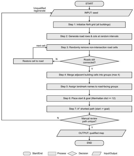
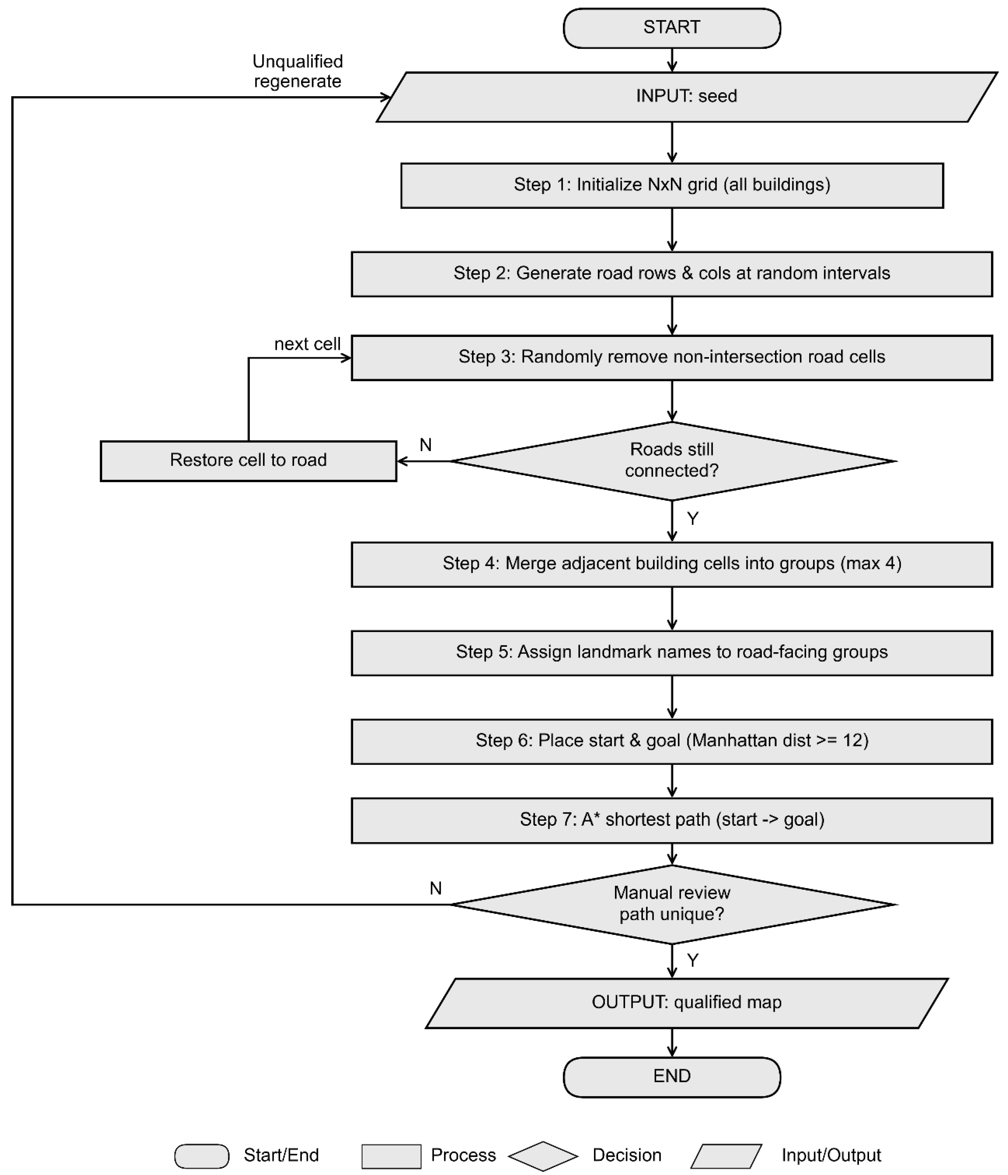
The map generator, as summarized in Figure 1, yielded reproducible city-like grid environments in which the collected instructions were grounded. A 20 × 20 grid was first initialized with every cell in the building state. Horizontal and vertical road lines were subsequently placed, with the gap between two parallel roads sampled uniformly from 2 to 4 grid cells. This produced an orthogonal skeleton where intersections were formed at crossing points. To break the skeleton regularity, non-intersection road cells were visited in random order, and each was tentatively returned to the building state. Upon every tentative removal, connectivity of the remaining road network was checked via breadth-first search, and a cell that would disconnect the network was restored to the road state before evaluation of the next candidate. This delivered a sparse but fully connected road network. Building cells remaining between the roads were merged by randomized agglomeration of 4-connected neighbors into groups of at most four cells, giving footprints of varied sizes. Every group with a road-facing side was then assigned a landmark name drawn from a predefined pool of roughly 90 Chinese names spanning catering, retail, medical, civic, educational, transport, and leisure categories. These named groups were the referents of the instructions collected later. Names were drawn without replacement until the pool was depleted. A20 × 20 map typically yielded more road-facing groups than the available name pool. Once the pool was exhausted, names were recycled, so a single label might appear twice within the same map. A start and a goal were then assigned to building cells adjacent to roads, subject to a minimum Manhattan distance of 12 to ensure sufficiently long routes. The shortest route between them was computed on road cells using A* [19]. The goal cell was admitted as a terminal walkable cell, given that start and goal were situated on building cells rather than road cells. A candidate map was accepted only if the route between the start and the goal was unique. Candidates with an ambiguous route were rejected and not used in the study. Re-checking all 50 accepted maps against this criterion confirmed that every one of them admitted exactly one route between the start and the goal. The uniqueness judgement was performed by the first author and not repeated independently. The criterion relied on a scripted shortest-path calculation, allowing reproducible regeneration using the released generator and map seeds. Landmark names could repeat within a map: all of the 50 maps contained at least one repeated name, and in the detect or stop commands of their ground truth, 191 of the 212 instructions referred to a name that occurred more than once on its map. These instructions were neither excluded nor disambiguated. Since the model had no access to the map, such ambiguity equally affected the ground truth and all tested models. All 212 ground-truth sequences reached their goal (Section 4.1).
Figure 1.
Map generation procedure (Y: Yes, N: No).
3.3. Robot Command Set
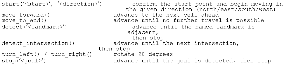
The command vocabulary covered eight members, each corresponding to an executable behavior feasible for a differential-drive robot equipped with landmark recognition (see Listing 1).
| Listing 1. List of robot commands. |
 |
3.4. Simulator and the path_reach Metric
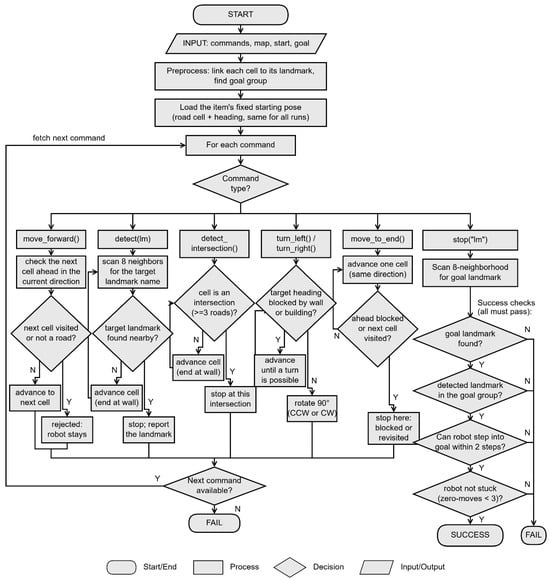
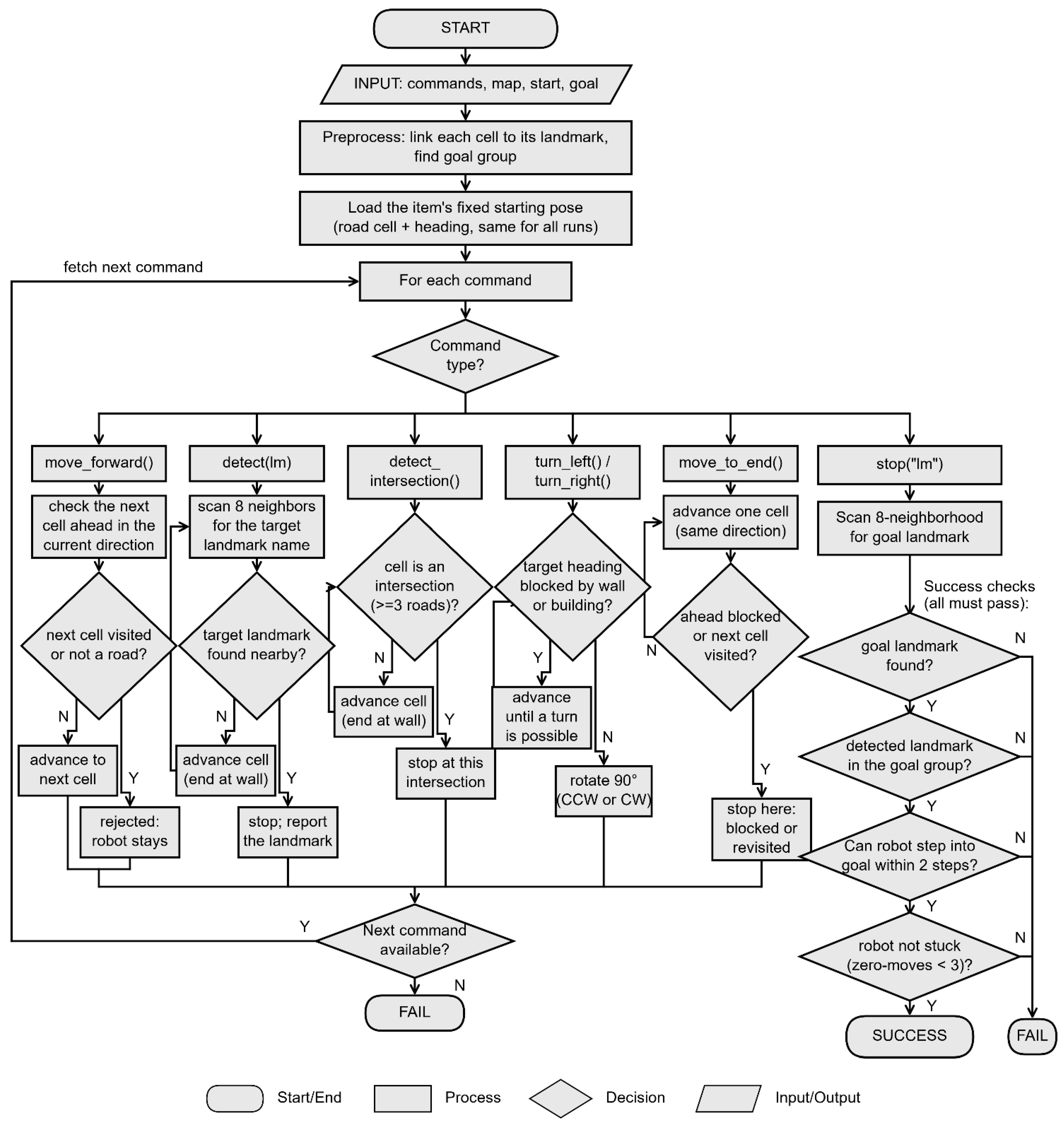
The simulator, as summarized in Figure 2, determined whether a command sequence produced by a model led the robot to the goal on the map. The raw model output was first parsed into a command list in two stages. Markdown code fences and reasoning-trace tags were stripped, and the remainder was parsed as JSON; if that parse failed, a regular-expression fallback extracted every substring of the form name(…), where name consisted of lowercase letters and underscores, and the parenthesized argument list contained no closing parenthesis. The fallback therefore recovered command tokens wherever they appeared in loosely formatted text, while a response lacking identifiable tokens yielded an empty command list. Moderately malformed output remained usable. The sequence must begin with a start command specifying the start landmark and the initial heading direction.
Figure 2.
Simulator control flow (Y: Yes, N: No).
In preprocessing, every building cell was linked to the landmark name of its group, and the goal group was identified from the goal cell. The starting pose (position and heading) for each sample was resolved in advance using only the map and the ground-truth annotation, prior to model inference. The heading carried by the start command of a generated sequence did not affect this initial placement. The pose was stored with the item and reused for the ground truth and all evaluated models, ensuring that every prediction for the same sample was tested from an identical starting state.
The remaining commands were consumed sequentially. Throughout execution, a global record of visited cells was maintained, and any move that would re-enter a visited cell was blocked. move_forward() advanced the robot into the front cell only when that cell was an unvisited road cell; otherwise, the command was rejected and the robot remained stationary. detect(‘<landmark>’) scanned the eight neighbors of the current cell and advanced one cell at a time until the landmark was detected or a wall was reached. detect_intersection() stopped at the first road cell with at least three road neighbors. turn_left() and turn_right() rotated the robot by 90°; if the new heading was blocked by a wall or a building, the robot first advanced along its current heading until the turn became feasible, as it could not physically rotate into a wall. move_to_end() advanced until the front cell was blocked or already visited. The transition semantics described above were those of the permissive mode, in which all hidden constraints were active; the strict variant disabled them and executed each command literally, as it was defined in the prompt. Verifying whether the detected building matched the sample’s goal was not enforced as an execution constraint; instead, it defined task success, and this check was retained under both evaluation modes. Formal transition semantics for both modes and accompanying unit tests are provided in Supplementary Materials (Table S1 and Section S3). Invalid outputs were handled as follows. A trial was marked as failed if no command could be extracted, or if the first command was not start(). A command that matched none of the defined forms was ignored, and execution continued. The failure taxonomy of Section 4.5 counted such outputs separately as invalid-command format failures. Given that the start pose was fixed per item, the start name and the heading written in start() were not used. Every command terminated: each forward loop stopped at a wall, a previously visited cell, or a landmark detection. An upper bound of 500 iterations was further enforced as a safeguard, with no wall-clock timeout imposed. Commands after a successful stop() were not executed, a start() not being the first command was ignored like any other unrecognized command, and stop() succeeded only at the goal building of the item: a different goal name, or another building sharing the goal’s name, did not end the trial.
The stop(‘<goal>’) command terminated execution and triggered a verification cascade. The robot first advanced until the named landmark was observed in its eight-neighborhood or the advance terminated. All of the following must then hold: (i) the goal landmark was present in the eight-neighborhood of the stopping cell; (ii) the detected landmark cell belonged to the goal group, which prevented misidentification caused by an identically named building that was not the goal; (iii) the goal building could be entered from the stopping position within two orthogonal steps and was not sealed, which prevented false arrivals in which the landmark was merely visible in the eight-neighborhood (e.g., diagonally across a wall while being physically unreachable); and (iv) the peak number of consecutive zero-displacement detections was below three, rejecting degenerate sequences that repeatedly detected a landmark at the same position without displacement. The trial was labelled SUCCESS only if all four conditions were satisfied; otherwise, it was marked FAIL. After executing each command, the subsequent command was retrieved if available. If the sequence terminated without a valid stopping action, the trial was labelled FAIL. Incomplete sequences and incorrect terminal states were thus both penalized. The primary metric, path_reach, was considered the percentage of test items whose generated command sequence reached the goal under this procedure. It was deliberately coarser than exact sequence match: two different sequences that successfully reached the goal were both counted as valid.
3.5. Data Collection
In this study, 50 maps were generated. Six participants were recruited via direct outreach and were unaffiliated with the research team; each received CNY 25 for their time. All six annotators were adults, nationals of China, and native speakers of Chinese. The instructions were dictated in Standard Mandarin and transcribed in standard written Chinese; no regional dialect was represented in the corpus. Maps were presented as images, with the start cell highlighted in green and the goal cell in red, so that participants could view the map and these two endpoints but were not presented any reference route. Participants were instructed to describe the route from the start to the goal using their own words. No vocabulary was suggested and no examples were shown, so the language was unprompted. Responses were audio-recorded and transcribed by the first author. The recordings were deleted as soon as the transcript had been checked against them, and no audio file was retained. Only the de-identified transcripts were kept and released: at transcription, each speaker was replaced by a code (P1–P6), and no name, age, occupation, or other identifying details was recorded, so the released instructions could not be linked to any participant. All six participants offered informed consent before each session. The consent covered the recording, the transcription, the deletion of the audio files, and the public release of the de-identified transcripts (see the Informed Consent Statement). As a result, 300 instructions were collected. Each instruction was first screened against the map; the screening assigned one or more of the five categories defined below, and an instruction was excluded when at least one of them applied. Screening and the subsequent translation of valid instructions into ground-truth command sequences were performed solely by the first author. No second annotator was involved in either step, so no adjudication step arose and inter-annotator agreement was not assessed for either. Out of the 300 instructions, 88 were removed under five operational categories: 50 were incomplete descriptions, 22 described a route not present on the map, 16 named a landmark incorrectly, 2 gave a clearly wrong turn direction, and none failed to mention the goal. The categories were not mutually exclusive: 86 instructions were removed for a single reason and 2 for two reasons. Accordingly, the category counts summed to 90, while 88 unique instructions were removed. Participant-wise exclusion statistics are reported in the Supplementary Materials (Table S5a–c), and the item-level exclusion log is provided in the repository (see the Data Availability Statement). Ultimately, the remaining 212 formed the corpus.
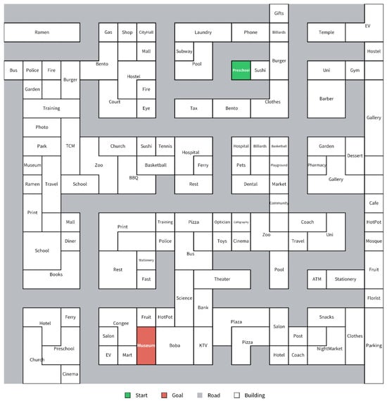
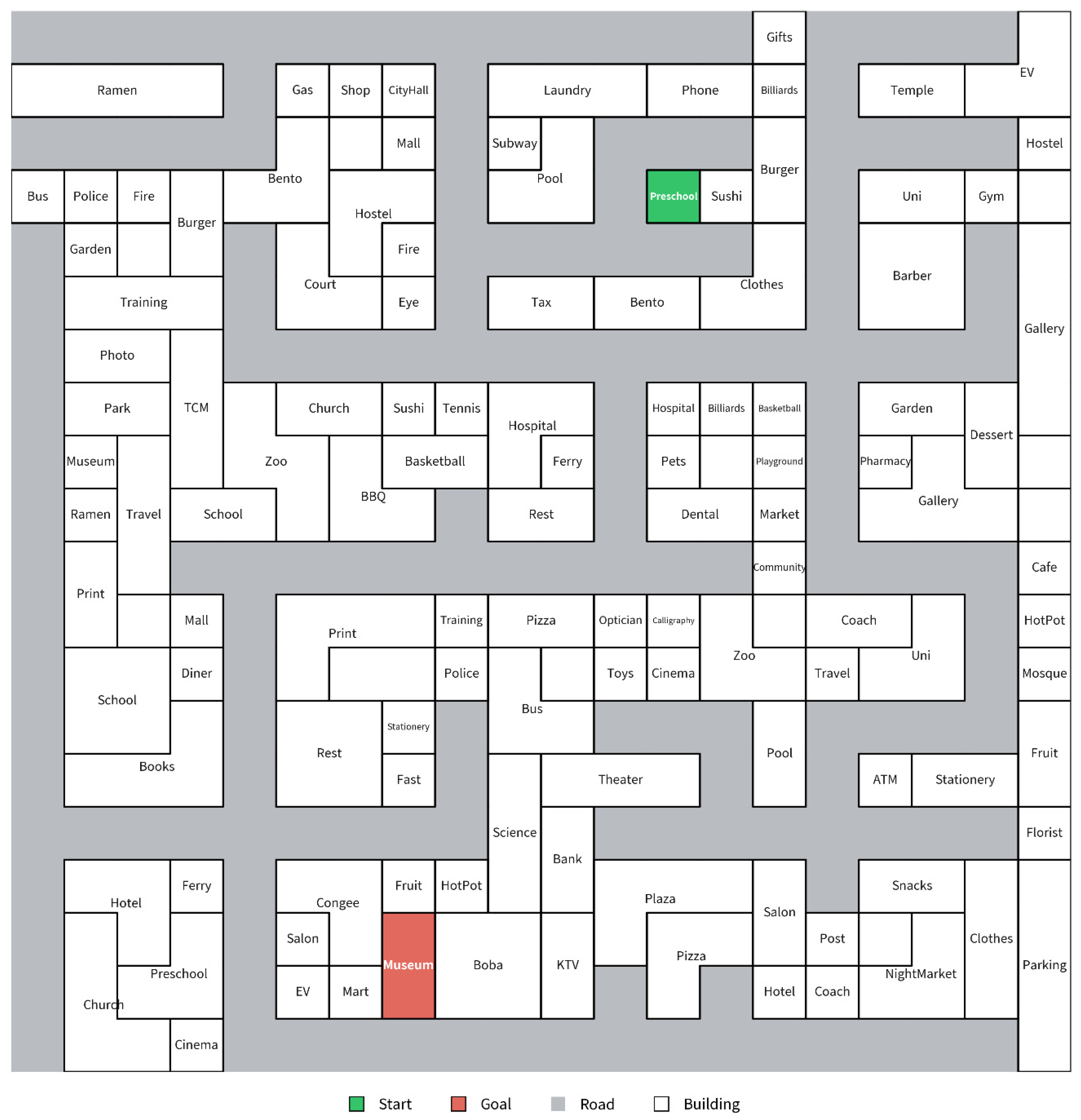
Figure 3 and Table 2 present a complete worked example. All six participants described the same route on the same map, from Preschool to Museum, yet they produced instructions that differed in length, vocabulary, and reference frame, which were expanded into command sequences ranging from 14 to 19 commands. The English translations were illustrative and shortened (… marks omitted passages), and the models received only the original Chinese text, as detailed in Supplementary Materials (Section S2). The final clause of P3, “right for 3/14 of the way”, could not be expressed in the command vocabulary; it was annotated as a turn towards map-right (turn_left() when heading south) followed by move_forward() and stop(‘Museum’), which advanced until the goal was detected. This verbal description aligned with the map layout: the final road segment spanned 14 grid cells, and the Museum was positioned 3 cells along this road.
Figure 3.
Example of a generated map with English landmark labels.
Table 2.
Instructions collected for the map of Figure 3 and ground-truth command sequences.
3.6. Corpus Statistics and Splits
The corpus contained a total of 212 instructions over 50 maps. Instructions averaged 78.3 characters (median 72, range 18–218), and ground-truth sequences averaged 15.0 commands (median 14, SD 7.0, range 4–42). Table 3 presents the command distribution.
Table 3.
Command frequency in the 212 ground-truth sequences (3172 commands in total).
The most consequential property of the corpus was that reference frame was determined by the participant, not by the map or the route. Table 4 shows the breakdown. Two participants relied entirely on egocentric descriptions, one used the map frame throughout, and three employed cardinal directions, of which two used cardinal references exclusively. Converting a cardinal instruction required tracking the robot’s heading through every preceding turn, whereas converting an egocentric one did not. The corpus therefore contained two quite different computational demands, distributed by the author rather than at random.
Table 4.
Reference-frame markers by participant. Cardinal: compass terms (east, west, south, north). Map frame: “up” and “down” used as directions, as in “walk down.” Egocentric: “left” and “right” used as directions, including “turn left,” “turn right,” “on the left-hand side,” and “on the right-hand side.” Words only inside a landmark name were not counted.
The corpus was partitioned on a per-map basis, such that each map belonged to only one split: 126 instructions over 30 maps for training, 21 over 5 for validation, and 65 over 15 for testing. Mean sequence length was comparable across splits (15.3, 13.9, and 14.7 commands). Participant proportions were approximately balanced, with P5 thinnest at 6–10% of each split. Since 32 of its 50 instructions were excluded, 30 of them were considered incomplete. Exclusions were not spread evenly across speakers: 16, 8, 11, 6, 32, and 15 instructions were removed for P1 to P6, leaving 34, 42, 39, 44, 18, and 35. Almost all of P3’s exclusions concerned routes that did not exist on the map, while almost all of P5’s involved incomplete descriptions. Accordingly, the corpus represented those two instruction styles weaklier than the others, and the per-participant results in Section 4.4 should be interpreted with that in mind.
3.7. Prompts
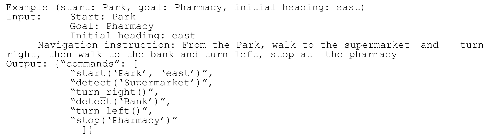
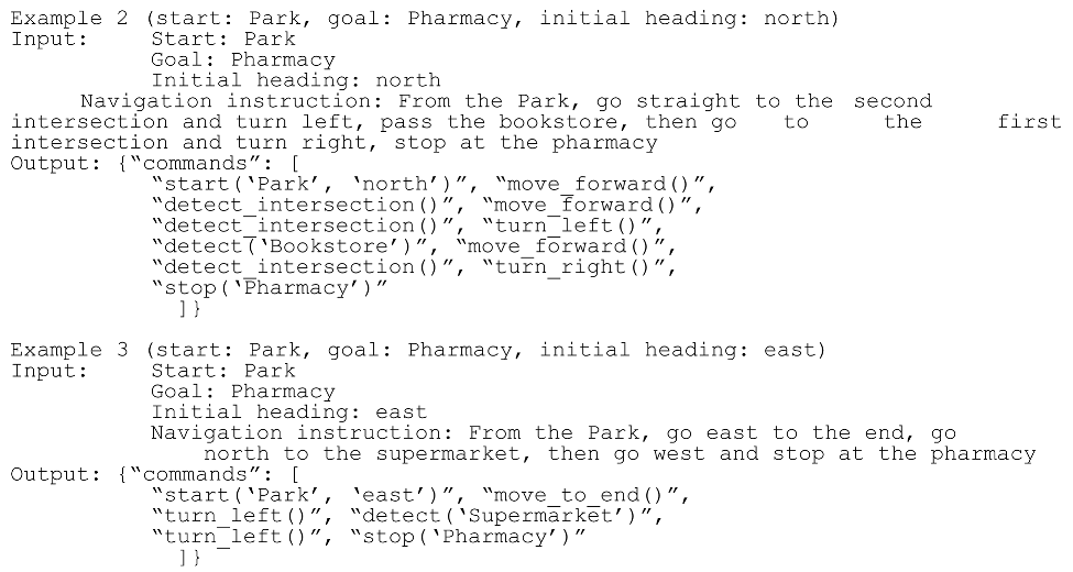
In this study, three system prompts were utilized, all sharing a character-identical block containing the command definitions, nine conversion rules, and the output-format specification (see Listings 2, 3, and 4). They differed in the number of worked examples appended (zero, one, and three). Example count was therefore the only variable. The prompts were written in Chinese, matching the language of the input. The worked examples were written by the authors, each illustrating a different group of conversion rules (Example 1: turns at named landmarks; Example 2: counted intersections; Example 3: walking to the end of a road and cardinal directions); their landmark names sourced from the same vocabulary as the corpus maps, but their routes did not occur in the corpus (no example start–goal pair appeared among the 212 instructions), so they shared command templates with the test items but none of their routes. Byte-level prompt files are provided in the repository (see the Data Availability Statement).
One characteristic of these prompts should be explicitly clarified, as it shaped the interpretation of subsequent results. The conversion rules did not state the no-revisit constraint that the simulator enforced in Section 3.4. However, the model could not act on such a rule even if it were stated, as it had no access to the map and had no representation of which cells it had passed. The constraint excluded no valid reference route, as all 212 ground-truth sequences executed successfully under it. However, a model that produced a re-visit route would be refused by the simulator without having been told. This applied identically to every model and every condition, so it did not confound comparisons between systems.
The block shared by all three prompts (English ver.) translated as follows.
| Listing 2. Prompt v0 (zero-shot, no examples). |
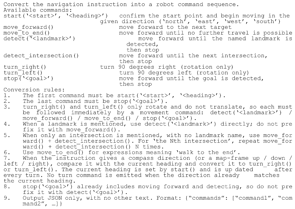 |
Prompt v0 ended there. Prompt v1 appended the single worked example below.
| Listing 3. Prompt v1 (one worked example). |
 |
Prompt v2 appended that example together with the two below, which added intersection counting and a longer route combining move_to_end() and repeated turns.
| Listing 4. Prompt v2 (three worked examples). |
 |
3.8. Models and Inference
Twelve models were hereby evaluated in three tiers, categorized by weight availability and parameter count, independent of deployment environment (Table 5). The two open-weight tiers were run under 4-bit quantization on a single GPU, except Gemma-2-9B, which was run in bf16 without quantization on an A100, as the 4-bit path could not be used for this checkpoint in our environment. The same limitation applied to its fine-tuning (Section 4.3). Thee third tier consisted of proprietary models accessed through provider APIs. All open-weight inference and all fine-tuning were carried out on Google Colab GPU instances, not on embedded or robot-mounted hardware. The tiers therefore characterized model classes, not measured on-device behavior, and no claim was made herein about latency, memory, or energy consumption on a physical robot. Each model received the system prompt and the instruction block as a user message via its own chat template.
Table 5.
Evaluated models.
Outputs were post-processed before parsing: reasoning-trace delimiters and Markdown code fences were stripped, the remainder was parsed as JSON, and a regular-expression fallback recovered command tokens following the name(…) pattern upon JSON parsing failure. Section 3.4 lists the same two-stage procedure, along with the precise patterns accepted by the fallback. All open-weight models were decoded greedily (do_sample = False, so temperature, top-p, and top-k did not apply; repetition penalty 1.05 for Qwen2.5-7B, from its released generation configuration, and none for the other models) with a cap of 512 new tokens, and the thinking mode of the Qwen3 models was disabled (enable_thinking = False). The cap did not cut off a correct answer: the longest ground-truth sequence was at most 168 tokens, and all 121 outputs reaching the cap had already failed (Supplementary Table S6). One model evaluated in the submitted version, DeepSeek-R1-Distill-Qwen-7B, was not part of the comparison reported herein: at this output budget, its results reflected truncation of the reasoning trace rather than route ability, so it was absent from Table 5 and all analyses below. Considering deterministic decoding, each model–prompt–item combination was generated once, and no output was regenerated after a failure. The proprietary models were queried with temperature 0 (Qwen3.7-Max, DeepSeek-V4-Pro), the provider default (Kimi-K2.7-Code, ChatGPT-5.5), top-p left at the provider default, and reasoning mode enabled (provider default for ChatGPT-5.5) on 3 August 2026 (dates in UTC; ChatGPT-5.5: 6 August 2026; second and third runs of Kimi-K2.7-Code and ChatGPT-5.5: 12 October 2026) through the providers’ OpenAI-compatible chat-completions APIs (Alibaba Cloud DashScope for Qwen3.7-Max and Kimi-K2.7-Code, the DeepSeek API for DeepSeek-V4-Pro, and the OpenAI Batch API for ChatGPT-5.5). Given that Kimi-K2.7-Code and ChatGPT-5.5 did not accept a temperature of 0, each was run three times on every prompt. All reported success rates for these models corresponded to the average across the three replicates, with run-level ranges presented where applicable. The paired analysis in Section 3.10 incorporated all three replicates. The other two were run once, and no proprietary output was empty. Token counts and context-window use are presented in Supplementary Table S6, and Supplementary Table S7 details checkpoint identifiers, parameter counts, licences, library versions, and provider model IDs.
3.9. Fine-Tuning and Low-Rank Adaptation
Prompt engineering could place only a handful of examples within the context window. To leverage the full set of 126 annotated instructions, the study also adopted task-specific fine-tuning as a second instruction-conversion paradigm.
Fine-tuning adapted a pre-trained model to a downstream task by continuing training on task-specific data. Current approaches generally fall into two categories: Full-parameter fine-tuning updates every weight in the model; at the scale of several billion parameters, this requires storing optimizer states and gradients for the entire parameter set, necessitating substantial computational cost [20]. Parameter-efficient fine-tuning (PEFT) instead updates only a small fraction of the parameters, typically by introducing additional trainable modules, while keeping the great majority of pre-trained weights frozen, which sharply reduces both computation and storage [20]. Low-Rank Adaptation (LoRA) [21] freezes all pre-trained weights and injects trainable low-rank decomposition matrices into selected layers of the transformer, recognized as a representative PEFT method. For a weight matrix W0 ∈ ℝ^{d × k}, LoRA constrains the update to ΔW = BA, where B ∈ ℝ^{d × r} and A ∈ ℝ^{r × k}, with rank r < min (d, k). Only A and B receive gradient updates, reducing the number of trainable parameters by orders of magnitude—typically to well under 1% of the base model—while leaving the representational capacity of the frozen base intact. Two considerations motivated the use of LoRA herein. First, with only 126 training instructions and four 8–9B architectures to cover, full-parameter fine-tuning was considered computationally impractical and, on a dataset of this size, prone to catastrophic forgetting [22] and severe overfitting [20]. LoRA mitigated all three concerns: its modest parameter budget enabled single-GPU training, the low-rank bottleneck limited overfitting, and freezing the base model eliminated forgetting. Second, the target behavior was primarily format adherence—emitting syntactically valid JSON command sequences terminated by stop()—rather than learning new factual or spatial knowledge, a use case well suited for LoRA.
3.10. Statistical Analysis
All 65 test samples were evaluated by every model under all prompt variants, yielding item-paired observations clustered by participant and map with heterogeneous performance across models. Counts pooled across models did not constitute independent observations. The prompt comparison was therefore analyzed as follows.
The unit of observation was the item: each item contributed one observation for every model–prompt–run combination: one run for the ten models run once, three runs for Kimi-K2.7-Code and ChatGPT-5.5. This delivered a total of 3120 observations from twelve models, three prompts, and 65 items (Section 3.8). (i) The primary analysis was a mixed-effects logistic regression of the binary item outcome on prompt and model, with random intercepts for item, map, and speaker, fitted by variational Bayes; it yielded conditional effect estimates with posterior credible intervals. (ii) As a frequentist reference showing consistently valid standard errors under an unknown within-item correlation, a generalized estimating equation (GEE) with a binomial mean model, the same fixed effects and clustering by item with robust standard errors yielded population-averaged odds ratios and 95% confidence intervals. (iii) The three prompt contrasts—one versus zero examples, three versus zero, and three versus one—were corrected for multiplicity with the Holm procedure. (iv) Paired comparisons within a single model were conducted via the exact McNemar test on the same items and reported as auxiliary evidence without correction. For the two models with three runs, the test was applied to each run separately.
Prompt comparisons therefore rested on these effect estimates rather than on pooled counts, and no equivalence claim was asserted.
4. Results
4.1. Validity of the Ground Truth
Before evaluating any model, all 212 ground-truth command sequences were executed in the simulator under the permissive execution used for all main results. Each reached its goal: 126/126 training, 21/21 validation, and 65/65 test, yielding an attainable ceiling on path_reach of 100%.
4.2. Results of Open-Weight and Cloud Models
None of the open-weight models within the 3–4B parameter tier achieved a success rate above 6.2% (Table 6). The best result in the open-weight 7–9B tier was 9.2% (6/65), achieved by Llama-3.1-8B under prompt v2 (Table 7). Doubling parameter count relative to the 3–4B tier yielded a maximum gain of only 3.1%, equivalent to two additional successful items. One entry should be qualified. Gemma-2-9B was the extreme open-weight case: only 2 of its 65 outputs under v0 were executable command sequences, against 26 under v1 and 40 under v2. Accordingly, its v0 cell reflected output discipline rather than navigation. In the cloud tier, only two of the 1560 outputs encountered a format problem (both from Kimi-K2.7-Code under v0), and both still reached the goal, so every cloud failure was a route error. The best cloud cell (Table 8) achieved 80.0% (52/65), against 9.2% (6/65) for the best open-weight zero-shot cell. The full failure taxonomy was further reported, as illustrated in Section 4.5.
Table 6.
path_reach (%) for open-weight 3–4B models, 65 test items. Successes in parentheses. Brackets give 95% Wilson score confidence intervals (%).
Table 7.
path_reach (%) for open-weight 7–9B models, 65 test items. Brackets give 95% Wilson score confidence intervals (%).
Table 8.
path_reach (%) for proprietary cloud models accessed by API, 65 test items. Brackets yielded 95% Wilson score confidence intervals (%); for Kimi-K2.7-Code and ChatGPT-5.5, which were run three times; cells gave the mean percentage and mean number of successes, and brackets the range of successes over the runs.
Within the open-weight tiers, the differences were one to two items under the three prompt conditions. Pooled over the five 7–9B models, v0 gave 14/325, and v2 yielded 22/325. Pooled over the four cloud models, v0 obtained 176.3/260, v1 gave 185.3/260, and v2 delivered 185.0/260. The largest single-model change was DeepSeek-V4-Pro, from 37 to 44 successes. Run-to-run variation was substantial: across its three runs, ChatGPT-5.5 exhibited a difference of up to four successful samples for a given prompt, while Kimi-K2.7-Code varied by up to six. The paired analysis of Section 3.10 did not detect a reliable effect of worked examples (Table 9): pooled path_reach rose from 25.0% with no example to 27.2% with one and 27.7% with three, yet every population-averaged odds ratio demonstrated a confidence interval that included 1 (Holm-adjusted p ≥ 0.247), and only the mixed-effects estimate for three versus zero examples had a credible interval excluding 1. Within single models, none of the 32 exact McNemar comparisons against zero examples (per run for the two models run three times) reached significance (smallest uncorrected p = 0.062).
Table 9.
Prompt effect estimates from the paired analysis specified in Section 3.10. The first block gave population-averaged odds ratios from the GEE clustered by item, with frequentist 95% confidence intervals; the last column yielded the conditional odds ratios from the mixed-effects model, with posterior 95% credible intervals. The three contrasts were the same 65 items under different numbers of worked examples, and the p values were Holm-corrected across the three contrasts. Kimi-K2.7-Code and ChatGPT-5.5 contributed all three of their runs, yielding a total of 3120 observations.
4.3. Fine-Tuning
Four open-weight 8–9B models were fine-tuned with LoRA on the 126 training instructions, using prompt v2 as the system message and the ground-truth JSON as the target. Hyperparameters were held constant across models: rank = 32, alpha = 32, dropout = 0, learning rate = 2 × 10⁻⁴, effective batch size = 16, maximum 10 epochs, linear schedule with 5% warmup, and seed = 42. Validation loss was computed every 5 steps on the 21 validation samples. Early stopping was triggered after 3 evaluations without improvement, and the optimal checkpoint was retained. Three of the four runs stopped early. All four runs exhibited the same shape: validation loss fell steeply to roughly step 20, flattened between 0.07 and 0.11, and then drifted upward, while the training loss kept decreasing until early stopping terminated training (Table 10). Gemma-2-9B was trained in bf16 on an A100 using the standard transformers and PEFT stack rather than the 4-bit path used for the other three, due to a loader incompatibility. Both configurations ran on Google Colab. LoRA adapters were attached to the q, k, v, o, gate, up, and down projections. For GLM-4-9B, where gate and up projections were fused into a single layer, adapters were attached only to the q, k, v, o, and down projections. This setup yielded 83.9 M trainable parameters for Llama-3.1-8B, 87.3 M for Qwen3-8B, 54.9 M for GLM-4-9B, and 108.0 M for Gemma-2-9B. The maximum sequence length was 2048 tokens. Optimizer AdamW was used (8-bit; 32-bit for Gemma-2-9B), with a weight decay of 0.01. The per-device batch size was 2 (GLM-4-9B: 1) with 8 (GLM-4-9B: 16) gradient-accumulation steps, resulting in an effective batch size of 16. Training precision was bf16 (Qwen3-8B: fp16). 4-bit NF4 quantization was enabled using Unsloth 2026.8.1 (Transformers 5.5.0, PyTorch 2.11.0); GPU used included NVIDIA T4 (Qwen3-8B), L4 (Llama-3.1-8B, GLM-4-9B), and A100 (Gemma-2-9B). Wall-clock training time ranged from 19 to 83 min per model. The checkpoint with the lowest validation loss was retained (load_best_model_at_end), and a single seed (42) was run per model. The rank and the number of epochs were chosen from two preliminary Qwen3-8B runs (rank 16 with 5 epochs and rank 32 with 10 epochs), which were compared on the test set under an earlier version of the annotation and the simulator (19/65 and 24/65 goals reached). Subsequently, the second configuration was applied identically across all four models, with no other hyperparameters modified. As this choice was informed by the test set, the fine-tuned results might carry a mild optimistic bias.
Table 10.
Fine-tuning outcomes. Best validation loss and the step at which it occurred, with the final step indicating the point at which training halted.
Fine-tuning produced the only large within-tier effect in the study. For Qwen3-8B, path_reach improved from 5/65 to 18/65. Across the four models, 81/260 fine-tuned successes against 20/260 zero-shot were obtained. Format failures—outputs that could not be parsed into an executable command sequence fell from 93 to 2 across the four models (92 of the 93 base failures were repaired, and one previously valid output was no longer valid after fine-tuning). Route failures did not fall in the raw counts, and they rose for all four models (Table 11). This comparison must, however, be interpreted jointly with the change in its denominator: once more sequences became parseable, route failures that could not previously be assessed became observable, thus making a paired, item-level analysis more informative relative to the aggregate counts. When the comparison was limited to items with valid outputs both before and after fine-tuning, route competence improved as well, with path_reach rising from 10–15% to 33–43%. The direction remained consistent for all four architectures, though the estimates rested on 39–44 paired items per model and should be regarded as indicative rather than definitive. The per-model category counts, the paired transition matrices for the four architectures, and the comparison on a fixed denominator are detailed in the Supplementary Materials (Tables S2–S4). The residual validation loss might reflect the surface imitation of shared route templates rather than the correctness of route content. The simulator recorded a single reason for route failures: failure to reach the goal. Thus, finer-grained classification of failure modes was hard to achieve.
Table 11.
path_reach for LoRA fine-tuned models on prompt v2. n = 65. Format failures refer to outputs that cannot be parsed into an executable command sequence (invalid JSON, invalid schema, an invalid command name or a missing terminal stop()); route failures correspond to valid sequences that do not reach the goal. Format failures, route failures, and successes are mutually exclusive and together exhaustive. Counts are from the paired item-level analysis under the fixed start pose (Supplementary Tables S2–S4).
4.4. Results by Participant
Given the distinct stylistic preferences across participants, the test set could be partitioned by P1 to P6. Table 12 reports path_reach on prompt v2, pooled across the models of each tier. Pooled attempts in a cell were answers by different models to the same items; they were thus not independent observations. The percentages were descriptive, and with as few as four test items for P5, the participant-level contrasts were indicative only. The pattern differed sharply between tiers. In the open-weight tiers, performance remained at a low level for every participant (at most 15.0%). The cloud tier peaked on P4 and P3, and was the lowest on P5, while the fine-tuned models inverted this ordering entirely: they solved most of P1 and P5 and almost none of the remaining four. Fine-tuning therefore did not raise performance uniformly. Its gain was concentrated on two of the six participants, and those two were the ones whose instructions mapped most directly onto commands.
Table 12.
path_reach (%) by participant on prompt v2, pooled over the models in each tier. Test items per participant are given in the second column. Each cell gives the percentage followed, in parentheses, by the number of successful items over the pooled number of attempts for that participant and tier. Figures over small item counts, P5 in particular, should be read as indicative only. Cloud cells average the three runs of Kimi-K2.7-Code and ChatGPT-5.5, so their counts can be fractional.
A leave-one-speaker-out check indicated that the tier ordering was not driven by any single participant. Removing each speaker in turn and recomputing the pooled rates left the ordering unchanged across all six folds: the open-weight tiers stayed between 3.1% and 5.7%, the cloud tier between 64.6% and 72.9%, and their gap between 59.2 and 68.5%, against 65.1% on the full set. The fine-tuned tier exhibited the largest performance swing: its success rate ranged from 18.9% when P1 was excluded to 36.5% when P4 was excluded. This pattern was consistent with the concentration suggested above: the fine-tuning gain appeared to follow the instruction style of two speakers rather than representing a uniform effect. These ranges rested on six speakers and 65 test items and were therefore indicative. They suggested that the reference-frame imbalance documented in Section 3.6 did not drive the tier comparison, yet they also limited the extent to which the fine-tuning result could be generalized beyond these speakers.
4.5. Execution Modes and Failure Taxonomy
The simulator executed commands in the permissive mode described in Section 3.4, marked by four active hidden constraints. Of the four, the no-revisit rule had already been discussed in Section 3.7, whereas the other three were not disclosed to the models. Table 13 reports the same runs executed strictly instead, that is, with every command executed exactly as defined by the prompt. Strict execution lowered the pooled success count from 704.7/2600 to 299.7/2600. The loss was concentrated among tiers handling longer navigation trajectories: the cloud tier fell from 546.7 to 211.7 successes, whereas the open-weight tiers experienced a reduction of fewer than 30 successful runs.
Table 13.
path_reach under permissive execution featuring active hidden constraints of Section 3.4 and under strict execution with each command executed literally as defined by the prompt. Each cell covers the same 65 test items, and the fine-tuned entries are the four LoRA checkpoints evaluated on prompt v2.
As shown in Table 14, the difference was attributed to the individual hidden constraints by disabling one at a time. Only the stop cascade worked against the evaluated models: removing it raised the pooled count from 704.7 to 736.7. As a result, an average of 32 of the 2600 executions failed, since the goal was visible but could not be entered. The other constraints acted in the opposite direction. Requiring a blocked turn to advance rather than rotate in place yielded 409.7 successes, and detecting landmarks in the eight-neighborhood rather than the four-neighborhood contributed 291.3. Both simplified the task rather than increasing its difficulty and thus favored the models instead of imposing stricter evaluation. The no-revisit rule changed a single execution. Disabling all four constraints together for strict execution left 299.7 successes, close to the 295 obtained when the turn rule alone was disabled, as that rule dominated the other three.
Table 14.
Success counts with one hidden constraint disabled at a time. Δ is the pooled count with all constraints active (704.7) minus the count for that configuration; a positive Δ means the constraint made the models fail more often.
As illustrated in Table 15, failures of output form were separated from failures of navigation, revealing that the two were not evenly distributed across tiers. Pooled over all runs, 91.6% of outputs could be parsed and 81.2% of those were executable. As a result, close to one execution in five never produced a sequence that could be attempted at all. The gap was concentrated within the open-weight tiers. In these tiers, 85.0% and 86.6% of outputs were parseable, yet only about two-thirds of the parsed sequences were executable. By contrast, nearly all outputs from the cloud tier were both parseable and executable (two exceptions in 1560 outputs). Among executable executions, the goal was reached in 36.2% of cases. When measured against all items, consistent with the path_reach in Section 4.2, the success rate for these runs fell to 27.1%. The tier comparison in Section 4.2 therefore mixed the two: part of the apparent gap between the open-weight and cloud tiers was a gap in output discipline rather than in spatial–linguistic conversion. The regular-expression fallback of Section 3.4 was worth isolating, as it was deliberately permissive. Re-scoring every run with the fallback disabled changes GLM-4-9B under v0 from four successes to none, Llama-3.2-3B under v2 from three to two, and one of the three Kimi-K2.7-Code runs under v0 by one success. No other cloud or no fine-tuned run was changed, so neither the tier ordering nor the tier best was affected. One entry in Table 7, however, rested entirely on the regex fallback parser.
Table 15.
Failure taxonomy under permissive execution. Each column is a stage of the funnel; percentages are relative to the denominator named in the column, and absolute counts are given in parentheses. A format failure is any output that fails one of the first three stages. The last column follows the path_reach convention used throughout, which executes any command sequence extractable, including through the regular-expression fallback, and ignores commands that match none of the defined forms. Therefore, it exceeds the conditional count (704.7 against 699.0 pooled): five successes rest on the fallback (GLM-4-9B v0, four; Llama-3.2-3B v2, one), and Kimi-K2.7-Code under v0 adds one success on the fallback in one of its three runs and one on an ignored invalid command in another. The per-model breakdown is provided in the repository (see the Data Availability Statement).
5. Discussion
5.1. Capability Tier Governing the Task
The dominant result was the size of the gap between model classes. Between the best 3–4B model and the best cloud model, the spread was 6.2% to 80.0%. Within the open-weight range, doubling from 3–4B to 7–9B parameters moved the ceiling by two test items. In this task, under these prompts, this quantization and this simulator, a route interface built from a 3–9B open-weight model with prompting alone succeeded on 9.2% of the test items. This figure characterized the tested configuration rather than the model class in general. This comparison demonstrated that the two classes differed by nearly an order of magnitude on a task for which both were given the same instructions and the same prompt. A natural-language route interface of this kind remained an unsolved challenge for smaller open-weight models.
5.2. Prompt Example Count Ablation
In this setting, the paired analysis detected no reliable effect of the number of worked examples: the pooled change was 2.2% from zero to one example and 2.7% from zero to three, both smaller than the variation in a single model between repeated runs. This should be particularly stated, as prompt engineering was widely treated as the primary lever available to practitioners [14]. One reading was that the examples carried information already available for the rules; another was that the fixed three-example budget used here was too limited to produce a measurable effect. Bode et al. [15] found the opposite result, arguing that a single worked episode was the most valuable single prompt component. However, their baseline prompt declared only function signatures, leaving the procedure to be inferred. Where the rules were already explicit, in-context examples yielded negligible gains. The experiment varied one prompt dimension only. Accordingly, no general claim was made that prompt engineering exerted no effect.
5.3. Fine-Tuning Repairing the Format
Fine-tuning improved format compliance in this study: most of the base models’ format failures were repaired, and the affected outputs became runnable. The raw route-failure counts did not fall, yet this was partly attributed to the changing denominator, as previously unparseable sequences could not be assessed for route correctness. When the comparison was restricted to items valid in both conditions, the same analysis pointed to a concurrent improvement in route competence (Section 4.3). This showed a practical implication. If the deployment constraint was that output must be machine-parseable and schema-conformant, then on this task, 126 supervised examples were ample and a 4-bit 8B model sufficed. If the constraint was that the robot must actually arrive, the evidence pointed in the same direction but was not yet conclusive at this sample size.
5.4. What Distinguished the Participants
Two structural properties of the instructions tracked these results. The first was the expansion from clause to command. P1 and P5 wrote at close to one command per clause, so converting their instructions relied largely on literal transliteration. The second property was landmark density. P4 and P6 named the most landmarks, about seven per test instruction. Among the five participants using landmarks, cloud performance roughly followed landmark density. P3 was the exception lacking any landmark anchor. It was the one participant whose cloud performance depended substantially on the prompt. Fine-tuned models succeeded at mechanically straightforward mapping cases, while cloud models performed better when landmarks constrained the route. P3 constituted the aforementioned exception to this pattern. These observations were made after result inspection and were not tested statistically, thus serving as exploratory hypotheses for future work rather than findings.
5.5. Limitations
First and most consequentially, this should be recognized as a simulation study, involving no physical robot, no sensor, and no actuator. The results characterized language-to-command conversion in isolation. In the real robot situation, there would be perception failures, odometry drift, or recovery behaviors, all of which a deployed system must handle. Extending the evaluation to a ROS 2 stack with real perception should be the next step.
Second, the test set covered 65 items. This was adequate for the tier comparisons, which were separated by tens of percentage points. However, its resolution was limited by the effects of a few percentage points: the pooled effect of worked examples, 2.2 to 2.7%, was not resolved by the paired analysis of Section 3.10, and differences of one or two successes within a single model could not be resolved either. Unparseable or non-executable outputs, such as those of Gemma-2-9B under prompt v0, made the corresponding figures uninformative for assessing underlying model competence.
Third, all open-weight inference was run on cloud GPU instances rather than on robot hardware. Hence, the study compared model classes, yet embedded latency, memory, or energy was not measured. Full accounting of the latency and bandwidth cost of API calls against self-hosted inference was still left to future work.
Fourth, the six speakers were recruited by personal approach rather than sampled from a defined population. The participant-to-participant spread reported in Section 4.4 revealed the outcomes’ dependence on instruction style; the towns, in turn, were regular 20 × 20 grids with a small vocabulary of landmark types, which were simpler in layout, scale, and visual complexity compared to real urban scenes. As a result, the performance reported here could not be generalized beyond these six speakers or beyond procedurally generated grid towns. Future work should extend the corpus to more speakers and to less regular environments.
Fifth, several further sources of bias should be recognized. The 88 excluded instructions removed erroneous and incomplete descriptions that a deployed system would encounter, so the corpus over-represented well-formed instructions. The hidden execution constraints of Section 3.4 were not disclosed to the models; Section 4.5 quantified their effect, but the permissive figures should be read with them in mind. The worked examples were written by the authors, yet similar route descriptions might also occur in the pretraining data of the evaluated models. Proprietary models might change behind a fixed name, so the cloud results were only valid for the access dates given in Section 3.8. Finally, the per-participant analysis in Section 4.4 was descriptive and carried no inferential statistics. In particular, the leave-one-speaker-out check was a sensitivity check on the same fixed test set: every model was evaluated on the same items, and none was retrained without the held-out speaker. It therefore did not constitute speaker-disjoint training and evaluation. It should thus not be read as evidence that the performance reported here generalized to unseen speakers.
6. Conclusions
This study introduced a corpus covering 212 free-form Chinese route instructions over 50 procedurally generated maps, each paired with an executable robot command sequence. Results verified that all 212 ground-truth sequences reached their goal in simulation. Using this 100% upper bound as reference, twelve large language models across three capability tiers were hereby evaluated with three prompt variants. Open-weight models in the 3–9B range achieved a maximum goal success rate of 9.2% in this evaluation; as a route interface for the task studied here, the evaluated open-weight configurations were not yet sufficient without further adaptation. Proprietary cloud models reached 80.0%, a gap of nearly an order of magnitude that was not narrowed by prompt example count in this study. Paired analysis detected no reliable effect of the number of worked examples (odds ratio: 1.15; 95% CI: 0.98–1.34; Holm-adjusted p ≥ 0.247). For this task, capability tier and supervised adaptation were considered the dominant influencing factors, whereas prompt example count was not a dominant factor based on the present evidence. LoRA fine-tuning on 126 examples raised mid-sized open models to 27.7–35.4%, and the gain spanned both output-format compliance and route competence.
Supplementary Materials
The following supporting information can be downloaded at https://www.mdpi.com/article/10.3390/jsan15060091/s1: Listing S1: Original Chinese prompt v0 (zero-shot, no examples); Listing S2: Original Chinese prompt v1 (one worked example); Listing S3: Original Chinese prompt v2 (three worked examples); Figure S1: The map shown to participants; Table S1: Transition semantics under permissive execution (main results) and strict (literal) execution; Table S2: Output categories for the base (zero-shot) and fine-tuned (FT) models, prompt v2, 65 test items per model; Table S3: Paired transitions between categories (rows: base model; columns: fine-tuned model); Table S4: Goal-reaching rate on a fixed denominator: test items yielding valid outputs both before and after fine-tuning; Table S5a: Instructions excluded during screening, by participant and exclusion category; Table S5b: Overlap of the exclusion categories; Table S5c: Unique exclusions by primary reason; Table S6: Token counts of the open-weight models (65 test items per prompt); Table S7: Evaluated models: checkpoints or provider model IDs, parameter counts, licences, context windows, alongside precision, quantization, and library versions.
Author Contributions
Conceptualization, R.Y. and Y.N.; methodology, R.Y. and Y.N.; software, R.Y. and Y.N.; validation, R.Y. and Y.N.; formal analysis, R.Y. and Y.N.; investigation, R.Y. and Y.N.; data curation, R.Y.; writing—original draft preparation, R.Y.; writing—review and editing, R.Y. and Y.N.; visualization, R.Y.; supervision, Y.N. All authors have read and agreed to the published version of the manuscript.
Funding
This research received no external funding.
Institutional Review Board Statement
This study is exempt from institutional review because the only interaction with the participants was an interview-type task (no intervention and no more than minimal risk) in which adult volunteers described routes shown on synthetic map images; no names, contact details, or demographic information were recorded. Participants were referred to only as P1–P6, and the responses therefore carried no identifiers. No deception was used, and no sensitive topics were raised.
Informed Consent Statement
Informed consent was obtained from all six participants. Before each session, the participants were given a full explanation of the study and agreed to (i) their participation and the use of their instructions, (ii) the audio recording of their instructions and its use for transcription, (iii) the deletion of the audio files once the transcription had been checked, and (iv) the public release of the de-identified transcripts. None of the participants requested data withdrawal.
Data Availability Statement
The corpus, map generator, simulator, evaluation script, prompt files, and raw model outputs are available at https://github.com/yuk1nishimura/zh-route2command/ (accessed on 5 November 2026). Inference, fine-tuning, and statistical procedures are described in Section 3.8, Section 3.9 and Section 3.10.
Conflicts of Interest
The authors declare no conflicts of interest.
References
- Deruyttere, T.; Vandenhende, S.; Grujicic, D.; Van Gool, L.; Moens, M.-F. Talk2Car: Taking Control of Your Self-Driving Car. In Proceedings of the 2019 Conference on Empirical Methods in Natural Language Processing and the 9th International Joint Conference on Natural Language Processing (EMNLP-IJCNLP), Hong Kong, China, 3–7 November 2019; pp. 2088–2098. [Google Scholar] [CrossRef] [Scilit]
- Sriram, N.N.; Maniar, T.; Kalyanasundaram, J.; Gandhi, V.; Bhowmick, B.; Krishna, K.M. Talk to the Vehicle: Language Conditioned Autonomous Navigation of Self Driving Cars. In Proceedings of the 2019 IEEE/RSJ International Conference on Intelligent Robots and Systems (IROS), Macau, China, 3–8 November 2019; pp. 5284–5290. [Google Scholar] [CrossRef] [Scilit]
- Ahn, M.; Brohan, A.; Brown, N.; Chebotar, Y.; Cortes, O.; David, B.; Finn, C.; Fu, C.; Gopalakrishnan, K.; Hausman, K.; et al. Do As I Can, Not As I Say: Grounding Language in Robotic Affordances. arXiv 2022, arXiv:2204.01691. [Google Scholar] [CrossRef] [Scilit]
- Liang, J.; Huang, W.; Xia, F.; Xu, P.; Hausman, K.; Ichter, B.; Florence, P.; Zeng, A. Code as Policies: Language Model Programs for Embodied Control. In Proceedings of the 2023 IEEE International Conference on Robotics and Automation (ICRA), London, UK, 29 May–2 June 2023; pp. 9493–9500. [Google Scholar] [CrossRef] [Scilit]
- Zhou, G.; Hong, Y.; Wu, Q. NavGPT: Explicit Reasoning in Vision-and-Language Navigation with Large Language Models. Proc. AAAI Conf. Artif. Intell. 2024, 38, 7641–7649. [Google Scholar] [CrossRef] [Scilit]
- Anderson, P.; Wu, Q.; Teney, D.; Bruce, J.; Johnson, M.; Sünderhauf, N.; Reid, I.; Gould, S.; van den Hengel, A. Vision-and-Language Navigation: Interpreting Visually-Grounded Navigation Instructions in Real Environments. In Proceedings of the 2018 IEEE/CVF Conference on Computer Vision and Pattern Recognition (CVPR), Salt Lake City, UT, USA, 18–22 June 2018; pp. 3674–3683. [Google Scholar] [CrossRef] [Scilit]
- Ku, A.; Anderson, P.; Patel, R.; Ie, E.; Baldridge, J. Room-Across-Room: Multilingual Vision-and-Language Navigation with Dense Spatiotemporal Grounding. In Proceedings of the 2020 Conference on Empirical Methods in Natural Language Processing (EMNLP), Online, 16–20 November 2020; pp. 4392–4412. [Google Scholar] [CrossRef] [Scilit]
- Kollar, T.; Tellex, S.; Roy, D.; Roy, N. Toward Understanding Natural Language Directions. In Proceedings of the 2010 5th ACM/IEEE International Conference on Human-Robot Interaction (HRI), Osaka, Japan, 2–5 March 2010; pp. 259–266. [Google Scholar] [CrossRef] [Scilit]
- Yan, A.; Wang, X.E.; Feng, J.; Li, L.; Wang, W.Y. Cross-Lingual Vision-Language Navigation. arXiv 2019, arXiv:1910.11301. [Google Scholar] [CrossRef] [Scilit]
- Artzi, Y.; Zettlemoyer, L. Weakly Supervised Learning of Semantic Parsers for Mapping Instructions to Actions. Trans. Assoc. Comput. Linguist. 2013, 1, 49–62. [Google Scholar] [CrossRef] [Scilit]
- Wake, N.; Kanehira, A.; Sasabuchi, K.; Takamatsu, J.; Ikeuchi, K. ChatGPT Empowered Long-Step Robot Control in Various Environments: A Case Application. IEEE Access 2023, 11, 95060–95078. [Google Scholar] [CrossRef] [Scilit]
- Espada, J.P.; Qiu, S.Y.; González Crespo, R.; Carús, J.L. Leveraging Large Language Models for Autonomous Robotic Mapping and Navigation. Int. J. Adv. Robot. Syst. 2025, 22, 17298806251325965. [Google Scholar] [CrossRef] [Scilit]
- Kim, Y.; Kim, D.; Choi, J.; Park, J.; Oh, N.; Park, D. A Survey on Integration of Large Language Models with Intelligent Robots. Intell. Serv. Robot. 2024, 17, 1091–1107. [Google Scholar] [CrossRef] [Scilit]
- Liu, P.; Yuan, W.; Fu, J.; Jiang, Z.; Hayashi, H.; Neubig, G. Pre-train, Prompt, and Predict: A Systematic Survey of Prompting Methods in Natural Language Processing. ACM Comput. Surv. 2023, 55, 195. [Google Scholar] [CrossRef] [Scilit]
- Bode, J.; Pätzold, B.; Memmesheimer, R.; Behnke, S. A Comparison of Prompt Engineering Techniques for Task Planning and Execution in Service Robotics. In Proceedings of the 2024 IEEE-RAS 23rd International Conference on Humanoid Robots (Humanoids), Nancy, France, 22–24 November 2024; pp. 309–314. [Google Scholar] [CrossRef] [Scilit]
- Das, M.; Hussain, Z.; Nawaz, M. Latency-Aware Benchmarking of Large Language Models for Natural-Language Robot Navigation in ROS 2. Sensors 2026, 26, 608. [Google Scholar] [CrossRef] [Scilit] [PubMed]
- Scholak, T.; Schucher, N.; Bahdanau, D. PICARD: Parsing Incrementally for Constrained Auto-Regressive Decoding from Language Models. In Proceedings of the 2021 Conference on Empirical Methods in Natural Language Processing (EMNLP), Punta Cana, Dominican Republic, 7–11 November 2021; pp. 9895–9901. [Google Scholar] [CrossRef] [Scilit]
- Dong, G.; Yuan, H.; Lu, K.; Li, C.; Xue, M.; Liu, D.; Wang, W.; Yuan, Z.; Zhou, C.; Zhou, J. How Abilities in Large Language Models Are Affected by Supervised Fine-Tuning Data Composition. In Proceedings of the 62nd Annual Meeting of the Association for Computational Linguistics (Volume 1: Long Papers), Bangkok, Thailand, 11–16 August 2024; pp. 177–198. [Google Scholar] [CrossRef] [Scilit]
- Hart, P.E.; Nilsson, N.J.; Raphael, B. A Formal Basis for the Heuristic Determination of Minimum Cost Paths. IEEE Trans. Syst. Sci. Cybern. 1968, 4, 100–107. [Google Scholar] [CrossRef] [Scilit]
- Ding, N.; Qin, Y.; Yang, G.; Wei, F.; Yang, Z.; Su, Y.; Hu, S.; Chen, Y.; Chan, C.-M.; Chen, W.; et al. Parameter-Efficient Fine-Tuning of Large-Scale Pre-Trained Language Models. Nat. Mach. Intell. 2023, 5, 220–235. [Google Scholar] [CrossRef] [Scilit]
- Hu, E.J.; Shen, Y.; Wallis, P.; Allen-Zhu, Z.; Li, Y.; Wang, S.; Wang, L.; Chen, W. LoRA: Low-Rank Adaptation of Large Language Models. arXiv 2021, arXiv:2106.09685. [Google Scholar] [CrossRef] [Scilit]
- Kirkpatrick, J.; Pascanu, R.; Rabinowitz, N.; Veness, J.; Desjardins, G.; Rusu, A.A.; Milan, K.; Quan, J.; Ramalho, T.; Grabska-Barwinska, A.; et al. Overcoming Catastrophic Forgetting in Neural Networks. Proc. Natl. Acad. Sci. USA 2017, 114, 3521–3526. [Google Scholar] [CrossRef] [Scilit] [PubMed]

Disclaimer/Publisher’s Note: The statements, opinions and data contained in all publications are solely those of the individual author(s) and contributor(s) and not of MDPI and/or the editor(s). MDPI and/or the editor(s) disclaim responsibility for any injury to people or property resulting from any ideas, methods, instructions or products referred to in the content. |
© 2026 by the authors. Licensee MDPI, Basel, Switzerland. This article is an open access article distributed under the terms and conditions of the Creative Commons Attribution (CC BY) license.