


Abstract
Determining the 3D position of a vehicle from a 2D image plays a key role in video surveillance, autonomous driving, and spatial localization. However, localization accuracy can significantly degrade in conditions of incomplete or synthetic measurement noise and keypoint jitter. In this paper, we propose a new iterative 3D position estimation algorithm (KGA). This algorithm includes geometric correction and calibration steps for converting from 2D to 3D coordinates; trajectory prediction and correction using a Kalman filter; and adaptive tuning of the filter parameters using the Goldschmidt algorithm. Experiments confirm that KGA outperforms the standard (FK) and modified (MFK) Kalman filters in accuracy and convergence speed, demonstrating robustness to various camera angles and noise levels. The novelty of this approach lies in the integration of the Goldschmidt algorithm into the Kalman filter to create an adaptation mechanism that dynamically adjusts the measurement noise covariance based on instantaneous innovation magnitude. Unlike end-to-end deep learning trackers or nonlinear filters (EKF/UKF), KGA is designed as a lightweight post-processing stage that can be seamlessly integrated into existing detection pipelines while maintaining the low computational footprint required for UAV-based edge deployment. The algorithm is of practical value for computer vision systems requiring accurate and robust tracking under varying observational conditions, with current implementation suitable for offline or buffered processing, and clear pathways to real-time deployment through code optimization. The algorithm is of practical value for computer vision systems requiring accurate and robust tracking under varying observational conditions.
1. Introduction
Modern tasks in intelligent transportation systems, autonomous driving, and traffic monitoring require highly accurate and reliable estimation of the spatial position of objects in real time [1]. One of the key problems in this area is determining and predicting the three-dimensional (3D) coordinates of a moving vehicle based on video stream data. Accurate knowledge of the 3D position, including 2D coordinates and depth, is critical for solving problems such as collision avoidance [2], trajectory planning [3], and road user behavior analysis [4]. Thus, object localization in 3D space is a key task in computer vision. In the field of intelligent video surveillance and driver assistance systems, the task of estimating the position of a vehicle based on video data is particularly relevant. This problem is complicated by data noise, instability in key point detection, and information loss [5]. In general, the problem of moving object detection is to reconstruct the precise 3D position (X, Y, Z) and state (velocity, acceleration) of a vehicle in the real world from a sequence of 2D camera images [6]. The main difficulty is that the camera projects the 3D world onto a 2D plane, losing depth information. Furthermore, video data is noisy, and object movements are not always predictable [7].
Thus, the main challenge facing researchers lies in the fundamental uncertainty [8] and noisiness of the data [9] obtained from video sources. Direct measurements provided by object detectors and pose estimation algorithms contain significant noise, caused by both camera hardware limitations [10] and the imperfections of computer vision algorithms [11]. Furthermore, the problem of estimating 3D position from a 2D image is fundamentally ill-posed and requires the use of additional information, such as camera calibration [12] and scene geometry data [13]. The presence of occlusions (object overlaps), challenging weather conditions, and dynamically changing environments further exacerbates this problem [14], leading to abrupt changes in measured coordinates (marker jitter) and track loss.
1.1. Motivation
To mitigate these difficulties, a number of solutions have been proposed in the scientific literature. Filtering algorithms, particularly the Kalman filter and its nonlinear modifications (e.g., the Unscented Kalman Filter) [15,16], are widely used to compensate for measurement noise and label jitter. These methods allow for an optimal (in terms of minimal mean square error) combination of the prediction of object dynamics with noisy observations, ensuring trajectory smoothing. For problems where the dynamic model is unknown or difficult to parameterize, window-based smoothing methods, such as the Savitzky–Golay filter [17], are effectively used. In the presence of short-term occlusions and measurement loss, these algorithms allow for extrapolation of the object’s position based on its previous motion.
To solve the fundamentally ill-posed problem of 3D reconstruction and combat persistent occlusions, approaches based on the use of a priori knowledge are used. These include methods using 3D models of objects [18] and constraints imposed by kinematics (e.g., constant skeletal link lengths in human pose estimation) [19]. Furthermore, a promising direction is the use of machine learning methods, in particular, deep neural networks [20], which are trained to predict 3D poses directly from 2D data by learning scene geometry and noise-robust features [21]. To improve reliability in complex conditions, multimodal systems are actively developing, combining data from multiple cameras [22] or integrating video with information from other types of sensors, such as lidar or IR cameras [23], which allows for overcoming the limitations inherent in each individual data type.
To overcome these difficulties, the scientific literature suggests the use of optimal filtering methods, among which the Kalman filter has demonstrated high efficiency. This algorithm allows for the optimal (in terms of minimum mean square error) combination of imprecise measurements with predictions based on a dynamic model of the object. Thus, the following methods can be used to solve this problem:
- Developing an adequate dynamic model of the vehicle that describes its motion in 3D space (e.g., a constant velocity or constant acceleration model).
- Creating a measurement model that links the internal state of the system (3D coordinates, velocity) with observed data (2D pixel coordinates, vehicle keypoints).
- Implementing a Kalman filter algorithm, which performs two main operations at each step: predicting the next state based on the dynamic model and correcting this prediction based on measurements received from the video stream. This allows not only smoothing noise but also predicting the object’s position during temporary tracking disruptions. The aim of this study is to develop and verify a method for estimating the 3D position of a moving vehicle in real time, based on the combined use of video stream data and a discrete Kalman filter. This paper proposes a specific structure for state and measurement models adapted for vehicle navigation tasks and experimentally evaluates its accuracy and robustness using real video data.
1.2. Our Contribution
The main results of our work can be summarized as follows:
- Development of an algorithm for determining the spatial position of a moving object in a video stream.
- Improvement in the accuracy of solving the problem of determining the spatial position of a moving object in a video stream using the developed algorithm.
- Improvement in the speed of solving the problem of determining the spatial position of a moving object in a video stream using the proposed algorithm. The proposed algorithm, based on the Kalman filter and the Goldschmidt algorithm, increased the accuracy of reconstructing the 3D position of a moving object compared to state-of-the-art methods, while minimizing the algorithm’s execution time. The proposed Kalman-Goldschmidt algorithm enables efficient adaptive tuning of the measurement noise covariance through scalar division via the Goldschmidt algorithm, offers computational efficiency by replacing expensive adaptive covariance estimation with a lightweight scalar iterative routine, while preserving standard matrix operations for state correction. This feature is demonstrated at the Kalman filter correction stage, namely, in the calculation of the Kalman gain. Next, we integrate the proposed algorithm to solve the problem of reconstructing the spatial position of a moving vehicle. Our algorithm achieves high accuracy values with fewer iterations than similar algorithms using a standard filtering algorithm.
1.3. Problem Statement
The core problem addressed in this work is the accurate estimation of the three-dimensional (3D) position and orientation of a moving vehicle from a sequence of 2D video frames captured by an unmanned aerial vehicle (UAV). This problem is challenging due to several factors:
- Loss of depth information: The camera projects the 3D world onto a 2D image plane, inherently losing depth information that must be recovered through geometric constraints or additional data.
- Measurement noise: Direct measurements from object detectors and keypoint extraction algorithms contain significant noise caused by camera hardware limitations, lighting conditions, and algorithmic imperfections.
- Dynamic environments: Vehicle motion, occlusions, and changing camera perspectives introduce additional uncertainty that complicates tracking and position estimation.
- Real-time requirements: Practical applications in traffic monitoring and autonomous driving require computational efficiency suitable for real-time or near-real-time processing on resource-constrained platforms.
Formally, given a sequence of 2D image frames with detected vehicle keypoints in each frame, and known camera calibration parameters, the goal is to estimate the 3D state vector at each time step , where represents position, represents velocity, represents orientation, and represents angular velocity. A detailed mathematical formulation of this problem is provided in Section 4, while the proposed solution algorithm is presented in Section 5.
The rest of the paper is structured as follows. Section 1.3 provides an overview of the problem statement, with a detailed mathematical formulation in Section 4. Section 2 reviews related work on methods for solving the problem of reconstructing the spatial position of a moving object. Section 3 describes the Kalman filtering algorithm and the Goldschmidt algorithm as background material. Section 5 presents the developed algorithm for determining spatial position. Section 6 presents the results of solving the problem of reconstructing the 3D position of a moving object. Section 7 discusses further improvements and areas of application of the proposed algorithm. Finally, Section 8 summarizes the paper and presents the conclusions. For ease of reading, the designations of this paper are listed in Table 1.
Table 1.
Introduced designations.
2. Related Works
Scope and Focus of the Literature Review:
This review centers on methods directly relevant to monocular UAV-based 3D vehicle localization. We prioritize works addressing: [24] geometric reconstruction from single-camera video, [25] adaptive filtering for dynamic state estimation under measurement uncertainty, [26] computational efficiency for resource-constrained platforms, and [27] UAV-specific challenges such as varying altitude and perspective. While some cited studies address broader contexts (e.g., multi-sensor fusion or ground-based systems), they are included to highlight methodological principles that inform our algorithmic design, such as noise modeling, convergence guarantees, and hardware-aware optimization.
2.1. General Overview
To process limited volumes of noisy data, the authors of [28] propose a real-time tracking algorithm based on L-shaped approximation, which determines the angles of moving vehicles. In [29], a Bayesian filter is used to estimate the position and size of a vehicle. To solve the same problem, the authors of [30] propose a modification of the SLAM method, which allows estimating the position and velocity of an object without any prior information about it. In [31], the researchers model the uncertainty of object localization during the detection process, represent the object locations as probability distributions in three-dimensional space, and collect and filter out redundant predictions about the object. In [32], the authors solve the problem of finding the maximum subgraph for the purpose of detecting 3D objects from mobile lidar point clouds. In the case of point cloud sparsity, the authors of [33] propose using a semantic and structural augmentation network for 3D object detection. A solution to the problem of temporal and spatial heterogeneity for individual objects by representing objects using a set of keyframes for each object and optimizing the spatial relationships between keyframes is presented in [34]. In [35], the authors propose matching 2D and 3D objects based on an algorithm that takes into account the distance constraint between the object’s surface and the rays projected back from the object’s contour. A number of studies integrate data obtained from Lidar and neural networks. For example, in paper [36], the YOLOv7 neural network is used to detect objects, and the obtained bounding boxes are further processed. Recent advances in deep learning-based perception have also improved traffic sign detection accuracy. For instance, an improved Sparse R-CNN architecture was proposed for autonomous vehicle applications, demonstrating enhanced detection performance under varying environmental conditions [37].
2.2. Kalman Filter
The Kalman filter is ideally suited for this task, as it allows one to predict the position of an object based on its dynamic model and adjust the prediction based on new, albeit noisy, measurements [38]. Research [39] confirms that even a basic implementation of the Kalman filter significantly outperforms a well-known system for determining the 3D position of a moving object [40], based on data from satellite navigation systems, in terms of accuracy and robustness. However, the classical Kalman filter is only applicable to linear systems, while vehicle kinematics, especially during maneuvering, as well as sensor models (e.g., a compass), are often nonlinear. This led to the use of the extended Kalman filter (EKF) architecture [41], which linearizes nonlinearities around the current estimate using a Taylor series [42]. However, its drawbacks—low accuracy with strong nonlinearities and the risk of divergence due to linearization errors—stimulate the search for alternatives. The Unscented Kalman Filter (UFK) [43] addresses these issues by using a deterministic choice of sigma points to approximate the state distribution. For highly nonlinear systems, such as a vehicle changing course abruptly, UFK exhibits greater accuracy and robustness than EKF, as shown in comparative studies, such as [44,45]. The work [46] focuses on solving a specific practical problem of working under non-stationary noise. For this, the authors apply the adaptive Kalman filter architecture. Another solution aims to use a cascaded or parallel architecture for this problem [47], where EKF or UFK is used to process the data, and then the output data is fused with new incoming data using a linear Kalman filter. This reduces the computational complexity. In the context of autonomous driving, UFK or quadratic Kalman filters have become the core for fusion with visual odometry data and lidar point clouds [48]. This allows for the creation of accurate local maps and positioning relative to them.
2.3. Positioning Within Modern Tracking Architectures
Contemporary 3D multi-object tracking (MOT) and 3D bounding box estimation increasingly rely on deep learning architectures, e.g., DeepSORT, ByteTrack, QD-3DT or nonlinear state estimators such as the Extended and Unscented Kalman Filters (EKF/UKF) [49,50]. While these methods achieve high accuracy in complex scenarios, they differ fundamentally in scope and computational profile from the proposed KGA.
DL-based MOT systems are end-to-end pipelines that combine object detection, feature embedding, data association, and state prediction [51]. Crucially, these architectures internally employ Kalman filtering for track maintenance and motion prediction. KGA is not designed to compete with detection or association components, but rather to serve as a drop-in replacement for the standard KF in such systems, offering faster convergence and improved robustness to measurement outliers without altering the upstream perception modules. Compared to EKF/UKF, which address nonlinear state dynamics through Jacobian linearization or sigma-point propagation, KGA assumes a linear constant-velocity motion model appropriate for short-horizon vehicle tracking. The geometric nonlinearity in our pipeline is explicitly resolved via vanishing point analysis and perspective-n-point (PnP) back-projection, decoupling projection errors from state dynamics. This design yields a significant computational advantage: EKF/UKF typically require 2–5 more floating-point operations per step due to Jacobian evaluation or sigma-point propagation, which conflicts with the strict latency and power constraints of UAV-based edge deployment. Furthermore, standard EKF/UKF implementations do not inherently adapt measurement noise covariance in response to instantaneous innovation magnitude, a capability central to KGA’s Goldschmidt-based adaptation mechanism.
2.4. Goldschmidt’s Algorithm
The problem of efficient division of floating-point numbers is a key one in the design of arithmetic logic units (ALUs) and mathematical coprocessors. Its complexity and computational cost motivate the search for alternative algorithms to slow sequential division (analogous to long division). Among iterative methods based on the multiplication principle, Goldschmidt’s algorithm [52] occupies a special place due to its simplicity and parallelizability. Goldschmidt’s algorithm and its iterative structure have proven preferable for many high-performance and vector processors. For example, research and practical implementations [53,54] have shown that Goldschmidt’s algorithm, especially when using pre-calculated high-precision initial approximations, can achieve higher throughput in pipelined execution units. In [55], the emphasis shifted to optimizing the algorithm for specific technological constraints and application areas. In [56], the authors use LUT tables in combination with linear or quadratic interpolation to obtain a first approximation with an accuracy of up to 10–16 bits, which reduces the number of required iterations to 1–2 for single precision and 2–3 for double precision. In [57], pipelined and fully combinatorial implementations of the Goldschmidt algorithm for FPGAs are studied, where its natural parallelism allows achieving high clock rates. In [58], the authors pay special attention to optimizing data formats (e.g., the logarithmic number system) and minimizing logical resources. Furthermore, the algorithm has found application not only for floating-point division, but also for calculating the inverse square root [59] and other reciprocals, which is critical in graphics processing units (GPUs) for geometric calculations and ray tracing, as well as in neural networks for normalization operations [60].
In addition to filtering-based approaches, optimization-based PnP solvers such as EPnP [61] and UPnP [62] remain widely used for single-frame 3D pose recovery from 2D-3D correspondences. While these methods are computationally efficient and do not require training data, they lack temporal consistency and are highly sensitive to keypoint detection noise. Recent advances in deep learning have introduced CNN- and Transformer-based architectures for direct 3D pose estimation from images or video sequences [63]. These methods achieve high accuracy in controlled settings but often require large annotated datasets, substantial GPU memory, and careful domain adaptation. The proposed KGA algorithm is designed to complement, rather than replace, such geometric or learning-based detectors by providing a lightweight, adaptive temporal filtering layer that improves stability and convergence in streaming scenarios.
Comparative Summary and Research Motivation:
To explicitly highlight the novelty and scientific contributions of the proposed approach, Table 2 provides a comparative analysis of the KGA algorithm against existing state-of-the-art methods for 3D vehicle localization.
Table 2.
Comparative analysis of methods for UAV-based 3D vehicle localization.
As shown in the comparison, while standard Kalman Filters (FK) offer low latency, they lack the adaptivity required for non-stationary video streams. Conversely, adaptive nonlinear filters (EKF/UKF) and deep learning-based trackers introduce significant computational overhead, making them unsuitable for resource-constrained UAV platforms. Single-frame solvers (e.g., EPnP) lack temporal consistency, leading to jitter.
The proposed KGA algorithm addresses this research gap by integrating a Goldschmidt-based scalar adaptation mechanism. This approach provides dynamic noise estimation with minimal computational overhead, effectively bridging the trade-off between estimation accuracy and hardware efficiency.
Based on the presented review of related works, we can draw conclusions about the limitations of existing solutions. Despite the existing methods presented in the cited studies, it can be concluded that some of them perform well in narrow, idealized conditions (small data volumes, linear models), but lose accuracy when faced with real-world nonlinearities, noise, and data sparsity. Other methods improve accuracy and stability, but at the expense of a sharp increase in computational load, which is critical for real-time systems on mobile platforms. Therefore, developing and verifying a highly efficient method for estimating the 3D position and dynamics of a moving vehicle in real time is a promising direction. The proposed algorithm in Section 5 aims to overcome the identified systemic shortcomings by synergistically combining video stream data and an optimized discrete Kalman filter adapted to handle the nonlinear kinematics of the vehicle.
Synthesis and Positioning:
The reviewed methods collectively underscore the trade-offs between accuracy, robustness, and computational load in monocular 3D tracking. Our proposed KGA algorithm builds upon these foundations by integrating geometric correction, adaptive Kalman filtering, and Goldschmidt-based scalar adaptation into a unified pipeline optimized for UAV deployment. The following sections detail how this integration addresses the limitations identified in the literature while maintaining compatibility with existing perception frameworks.
3. Materials and Methods
3.1. Kalman Filter
The Kalman filter is an optimal digital data processing algorithm that solves the problem of estimating the state of a dynamic system from a series of imprecise and noisy measurements. The key idea of the algorithm is to combine two sources of imprecise information, predicting the system’s state based on its previous state and a known model, as well as sensor measurements. The filter “weights” these two sources based on their estimated accuracies (covariances) to obtain the best possible estimate of the system’s true state.
Assuming that the system’s state changes according to a linear stochastic equation and the measurements are a linear function of the state, then Formula (1) expresses the process model, and (2) the measurement model:
The noises and are assumed to be independent of each other and of the state. The entire Kalman filter algorithm is an iterative process that performs two steps:
- Prediction: At this stage, the system predicts its next state (3) and the uncertainty (covariance) (4) of this prediction.
- Update: When a new measurement arrives, the filter “updates” the forecast using the real data, calculates the Kalman gain (5) and refines the state estimate (6) and covariance (7).
This cycle (prediction and correction) is repeated for each new measurement, allowing the filter to continually refine its estimate of the system’s state, effectively filtering out noise.
3.2. Goldschmidt’s Algorithm
The purpose of Goldschmidt’s algorithm is to calculate the quotient without division, using iterative refinement. This solves the problem of replacing division with multiplication. It is necessary to find a factor such that the denominator tends to 1, while the numerator tends to the desired quotient . The algorithm iteratively calculates the sequence of factors and updates the values and as follows:
- Initialization: calculating a rough approximation
Initial Approximation Selection: In our implementation, the initial approximation is chosen using a constant approximation approach where . This is sufficient for our application because the denominator (representing the squared innovation error ) is naturally bounded within the range due to normalization of measurement residuals in the Kalman filter.
For general applications where D may fall outside this range, G0 can be obtained through:
- Lookup table (LUT): Pre-computed values based on the exponent bits of .
- Linear approximation: , where coefficients are optimized for the expected input range.
- Bit manipulation: Using the floating-point representation to extract an initial estimate from the exponent.
Impact of Initial Guess Quality: Due to the quadratic convergence property of the Goldschmidt algorithm, the impact of an imperfect initial approximation is minimized within 2–3 iterations. The error at each step is squared (εi+1 = εi2), which means that even with a relatively poor initial guess (e.g., G0 with 50% error), the algorithm converges to machine precision within 4 iterations. In our experimental validation, we tested different G0 values (0.5, 1.0, 1.5) and confirmed that all configurations achieved the convergence threshold |Di − 1| < 10−6 within 3–4 iterations for our video stream data.
- 2.
- Calculating iterations (for )ifthen .
The error is squared at each step (quadratic convergence). Termination criterion: The iterative process terminates when one of the following conditions is satisfied:
- Convergence threshold: , where
- Maximum iteration limit: , where
The first condition ensures that the denominator converges to unity with sufficient numerical accuracy. The second condition guarantees bounded computational time for real-time applications on resource-constrained UAV platforms. Due to the quadratic convergence property ( is squared at each step), the convergence threshold is typically reached within 3–4 iterations for the measurement noise levels encountered in our video stream data.
Since and are multiplied by the same , their ratio is constant:
Clarification on Matrix Operations: It is important to distinguish between the scalar division performed by the Goldschmidt algorithm and the matrix inversion required for Kalman gain calculation. The Goldschmidt algorithm computes a scalar adaptive parameter:
where is the squared innovation error (a scalar value). This parameter is then used to scale the measurement noise covariance matrix:
The Kalman gain is subsequently calculated using standard matrix operations:
Thus, the Goldschmidt algorithm does not replace matrix inversion directly. Instead, it provides an efficient mechanism for adaptive covariance tuning based on measurement reliability. The computational benefit arises from:
- Fast scalar division with quadratic convergence (3–4 iterations)
- Adaptive adjustment without additional matrix decompositions
- Reduced sensitivity to innovation outliers through dynamic scaling
3.3. Formalization of the Goldschmidt Algorithm and Integration of the Kalman Filter
Although the classical Kalman filter provides optimal state estimation under Gaussian noise assumptions, its performance degrades when the measurement noise characteristics dynamically change. In real-world video streams, such changes often occur due to lighting changes, partial occlusions, and sudden object movements. To address this issue, we formalize the integration of the Goldschmidt algorithm as an adaptive mechanism that dynamically adjusts the filter gain based on the measurement reliability.
Computational bottleneck in the Kalman filter: The standard calculation of the Kalman gain requires matrix inversion according to Equation (5). This operation has a computational complexity of which becomes unacceptable in real-time applications, especially on resource-constrained UAV platforms.
Adaptive parameter formulation: Instead of direct matrix inversion, we introduce a dynamic adaptation parameter which modulates the covariance matrix of the measurement noise:
where is the sensitivity coefficient, and denotes the square of the innovation (forecast error). This parameter effectively scales the filter’s confidence in the measurements compared to the forecasts. Goldschmidt integration: Here, the innovation error serves as the initial denominator for the Goldschmidt process described in Section 3.2. The algorithm iteratively refines the correction factor until the internal error converges to zero. Thus, represents the input reliability metric, while represents the computed adaptive gain factor. The adaptation parameter is efficiently calculated using the Goldschmidt algorithm:
- Initialization:
- Iterative refinement for to :where
- Rapprochement: . Note: within the Goldschmidt loop, index refers to the iteration number, distinct from the global time step .
This approach achieves quadratic convergence, reducing the computational complexity from to per iteration, while for practical implementation only 3–4 iterations are required to achieve sufficient accuracy .
Calculation of the adaptive gain: the calculated parameter is taken into account when calculating the Kalman gain:
This formalization provides a theoretical basis for the algorithm described in Section 5, demonstrating how Goldschmidt’s algorithm achieves computational efficiency while maintaining estimation accuracy through adaptive parameter tuning.
Architectural Distinction of Computational Steps:
It is essential to clarify that the Goldschmidt algorithm does not replace the matrix inversion required for Kalman gain computation. Instead, it decouples the adaptation mechanism into three distinct stages:
- Scalar reciprocal computation: At each time step , the squared innovation magnitude is computed. The Goldschmidt algorithm iteratively refines the adaptive scaling factor using only three scalar multiplications and one subtraction per iteration. Quadratic convergence ensures machine precision in 3–4 iteratios.
- Adaptive covariance scaling: The scalar factor is applied to the nominal measurement noise covariance matrix: . This step dynamically modulates the filter’s confidence in measurements based on instantaneous reliability.
- Standard matrix operations for Kalman update: The Kalman gain is computed using conventional matrix algebra:. The matrix inversion remains intact but operates on an adaptively conditioned covariance matrix.
The computational advantage of KGA arises not from eliminating matrix inversion, but from replacing costly adaptive covariance estimation procedures, e.g., sliding-window statistics or iterative matrix decompositions with a lightweight, branchless scalar routine. This reduces the adaptation overhead from or to per step, while improving numerical conditioning and convergence speed.
Computational Efficiency Analysis:
The integration of the Goldschmidt algorithm introduces minimal overhead because it operates on a scalar innovation metric rather than on matrices. Each Goldschmidt iteration requires only three scalar multiplications and one subtraction; with quadratic convergence, 3–4 iterations suffice for machine precision. Thus, the additional cost is approximately 12–16 floating-point operations per time step.
In contrast, the dominant cost in the Kalman filter update is the inversion of the innovation covariance matrix , which requires operations ( FLOPS for using Cholesky decomposition). The state propagation and covariance update terms scale as with . Therefore, the Goldschmidt overhead constitutes less than of the total per-step computational load.
The performance gain of KGA arises not from reducing per-step complexity, but from accelerating convergence to the target accuracy. By adaptively scaling based on measurement reliability, the filter reaches steady-state estimation error in fewer time steps, as demonstrated in Section 6. This “time-to-accuracy” metric is more relevant for real-time video processing than raw FLOPS per frame.
3.4. Hardware-Oriented Complexity Analysis
The Goldschmidt algorithm offers several architectural advantages that make it particularly suitable for hardware-constrained deployment:
- Operation type: Each Goldschmidt iteration requires only three scalar multiplications and one subtraction. On modern embedded CPUs, e.g., ARM Cortex-A series, these map directly to fused multiply-add (FMA) instructions, which execute in a single cycle on pipelined units. In contrast, a hardware division instruction typically requires 20–40 cycles and may stall the pipeline.
- Branchless execution: The iterative refinement loop contains no conditional branches, enabling predictable execution and efficient instruction-level parallelism. This is critical for real-time systems where worst-case execution time (WCET) must be bounded.
- Quadratic convergence: The error is squared at each step meaning that machine precision is achieved in 3–4 iterations regardless of the initial approximation quality. This bounded iteration count allows static scheduling on hardware accelerators.
- Fixed-point compatibility: Since the algorithm operates on normalized scalar values in our implementation, it can be efficiently implemented in fixed-point arithmetic on DSPs or FPGAs, avoiding the area and power overhead of floating-point units.
- Memory efficiency: The scalar adaptation parameter requires only a single register, whereas adaptive covariance estimation via sliding windows would necessitate buffering elements, increasing memory bandwidth pressure.
Quantitative estimate: Replacing a scalar division ( cycles on ARM Cortex-A53) with 4 Goldschmidt iterations ( FMAs cycles) reduces the adaptation step latency by When combined with the avoidance of matrix decomposition for adaptive Rk tuning, the overall per-frame computational savings are estimated at 15–25% on embedded platforms, as reflected in the enhanced complexity breakdown.
4. Statement of the Problem
Based on the presented review of related works, we can draw conclusions about existing problems and dissatisfaction with the current state of solutions for this problem. Despite the existing methods presented in the cited studies, it can be concluded that some of them perform well in narrow, idealized conditions.
This section provides the detailed mathematical formulation of the problem introduced conceptually in Section 1.3. While Section 1.3 outlines the core challenges and research objectives at a high level, this section presents the formal equations and state-space representations required for algorithm implementation.
Let us formulate the problem of determining the 3D position of a car over time (its orientation and position) in a series of images, given the 2D images and the car model. To do this, we first find the rotation matrix and the position vector , given pairs of corresponding points and the parameters of the camera’s internal calibration matrix . Pairs of corresponding points define 3D points in the world coordinate system: , as well as their images on the camera plane .
In this case, the following relationship will be fulfilled:
The calibration matrix of the internal parameters of the camera will have the form:
Then this algorithm will consist of performing the basic steps of normalization and solving the problem of restoring the position of an object by points.
In the normalization step, 2D points are converted into normalized coordinates:
Then the equation will be written as:
The next step is to solve the optimization problem:
where
Afterwards, and reconstructed for each video frame, and the case with the largest number of inliers is selected. The algorithm’s output values will be matrices characterizing the camera rotation, the camera’s position in the world coordinate system, and the indices of the inlier points. The final camera model will be defined as:
In the world coordinate system, the projection of each 3D point can be represented as:
where , , .
Since the 3D position of the car is tracked over time, we then denote the state vector:
The state vector has a total dimensionality of 12 elements, structured as four 3-dimensional sub-vectors: —3D position coordinates in world frame; —linear velocity components; —orientation (Euler angles: roll, pitch, yaw); —angular velocity components.
Accordingly, the state transition matrix in Equation (19) is a 12 × 12 matrix that propagates all 12 state variables through time. The block-diagonal structure of F reflects the coupling between position-velocity and orientation-angular velocity pairs, while maintaining independence between translational and rotational dynamics in the linear approximation.
Let the system be discrete in time with a sampling step of . Then, taking into account the state transition matrix and the processor noise we write:
If we assume the model is linear, then the standard equations for the Kalman filter are written as follows:
For state prediction:
To update the status:
where is the Kalman gain, is the observation matrix obtained based on the numerical linear approximation , is the state covariance.
Equations (3)–(10) form the basis for constructing an iterative procedure for estimating the position of a moving object at a given moment in time. The complete algorithm for determining the spatial position of a moving object is presented in the next section.
5. Proposed Algorithm
In the modern problem of estimating the 3D pose of moving objects from 2D video data, key challenges remain sensitivity to camera calibration and scene geometry, error accumulation during dynamic object motion, and the tradeoff between computational complexity and accuracy. The algorithm proposed in this paper combines geometric scene correction, a Kalman filter, and an adaptive mechanism based on the Goldschmidt algorithm to address these issues.
The Kalman-Goldschmidt Algorithm (KGA) consists of three distinct phases: (1) camera calibration and geometric correction, (2) 3D back-projection and initial state estimation, and (3) Kalman filtering with Goldschmidt-based adaptive tuning. Each phase is described in detail below, with corresponding line numbers referencing Algorithm 1.
| Algorithm 1: Kalman-Goldschmidt Algorithm for 3D Vehicle Position Estimation |
| Input data 1: 2: 3: 4: 5: 6: 7: 8: 9: 10: PHASE 1: CAMERA CALIBRATION & GEOMETRIC CORRECTION 11: 12: 13: 14: 15: , 16: 17: 18: 19: 20: PHASE 2: 3D BACK-PROJECTION & INITIAL STATE 21: if then 22: 23: 24: 25: PHASE 3: KALMAN FILTERING WITH GOLDSCHMIDT ADAPTATION 26: 27: 28: 29: for 30: , 31: for 32: 33: 34: if then stop 35: 36: 37: 38: 39: Output data: 40: 41: 42: Output data: 43: |
5.1. Phase 1: Camera Calibration and Geometric Correction (Lines 11–20)
The first phase establishes the geometric relationship between 2D image coordinates and 3D world coordinates through vanishing point analysis. Vanishing Point Derivation: Given two pairs of parallel lines in the scene (e.g., vehicle edges), we compute their vanishing point as follows:
Line 1: through points and .
Line 2: through points and .
Line equations: , where , , .
Vanishing point (line intersection):
This is NOT a forward projection but rather a geometric intersection of two line projections in the image plane. The vanishing point represents where parallel lines in 3D space appear to converge in the 2D image due to perspective projection.
Focal Length Estimation: Using the vanishing point and optical center :
The optical center is obtained from pre-calibration (K matrix) or approximated as the image center , .
Intrinsic Matrix Formation:
Radial Distortion Correction:
The radial distortion parameters reported in Table 2 are actively used to correct image coordinates before geometric processing. Following the Brown-Conrady distortion model, each detected keypoint is undistorted to obtain normalized coordinates as follows:
where are normalized coordinates relative to the principal point. This undistortion step is applied as a preprocessing operation in Phase 1 of Algorithm 1, ensuring that subsequent vanishing point estimation and 3D back-projection operate on geometrically consistent coordinates that satisfy the pinhole camera model assumptions.
Robustness Analysis of Vanishing Point Estimation:
The vanishing point-based focal length estimation assumes scene parallelism and a stable optical center. In practice, camera tilt, lens distortion, or vehicle misalignment relative to the road direction can displace the computed vanishing point. A displacement of 50 pixels in a 1920 × 1080 frame typically introduces a 5–8% deviation in the estimated focal length, which propagates proportionally to depth estimation errors. To mitigate this sensitivity, our implementation incorporates three robustness mechanisms:
- Outlier rejection: Line fitting employs RANSAC to discard non-parallel or poorly detected edges, ensuring that only geometrically consistent structures contribute to the vanishing point computation.
- Temporal smoothing: The vanishing point coordinates are averaged across a sliding window of 5 consecutive frames, which suppresses transient biases caused by momentary perspective shifts or partial occlusions.
- Kalman prediction fallback: When geometric calibration drifts, the Kalman filter’s prediction step temporarily dominates the state update, relying on the vehicle’s dynamic model rather than noisy projections. The adaptive Goldschmidt mechanism further reduces measurement weight when reprojection errors spike.
Empirical validation with synthetic ±50 pixel vanishing point perturbations confirms that the initial 3D errors 0.25 m converges to 0.12 m within 3 frames, demonstrating that the KGA pipeline remains stable under moderate geometric uncertainties typical of UAV video streams.
5.2. Phase 2: 3D Back-Projection and Initial State Estimation (Lines 21–25)
World Reference Frame Definition. We define the world coordinate system as follows: origin: road surface directly below the camera at the initial frame; -axis: direction of vehicle motion parallel to road; -axis: lateral direction perpendicular to motion; -axis: vertical direction upward, perpendicular to the road surface.
Camera Localization. The camera extrinsic parameters are obtained by solving the perspective-n-point (PnP) problem using known object height :
where s is the scale factor are pixel coordinates, and are world coordinates. Given the known vehicle height , we can recover the camera position relative to the vehicle.
Initial State Acquisition. The initial state vector is obtained from the first frame’s geometric reconstruction:
where : 3D position from back-projection; : initial velocity (assumed stationary or from optical flow); : initial orientation (yaw from vanishing point direction); : initial angular velocity.
5.3. Phase 3: Kalman Filtering with Goldschmidt Adaptation (Lines 26–42)
The third phase implements the recursive state estimation with adaptive noise tuning.
Prediction Step:
where is the state transition matrix and is the process noise covariance.
Goldschmidt Adaptation (Lines 29–36):
Scalar innovation error:
Scalar reciprocal computation: via 3–4 Goldschmidt iterations
Adaptive covariance scaling:
Matrix operations:
State update: ,
The Goldschmidt algorithm provides efficient computation of with quadratic convergence (3–4 iterations), enabling real-time adaptive tuning without additional matrix decompositions.
Thus, the proposed algorithm combines geometric stability (via the vanishing point), dynamic filtering (via the Kalman filter), and adaptivity (via the Goldschmidt algorithm). This enables more accurate and stable 3D position estimation in real time under changing observation conditions, as confirmed by both the mathematical analysis and the algorithmic structure presented below (Figure 1).
Figure 1.
Scheme of the algorithm for determining the 3D position of a moving object.
Thus, the developed algorithm is a practical implementation of an approach aimed at overcoming the limitations identified in the literature review: it combines a nonlinear geometric projection, a Kalman filter for noise smoothing and dynamic estimation, and an adaptive correction mechanism for managing computational accuracy. To verify whether this architecture achieves the stated goal for real-time operation, an empirical study of its performance is necessary. The next section describes experimental simulations that evaluate the position accuracy, robustness to input noise, and computational performance of the algorithm.
Thus, the developed algorithm is a practical implementation of an approach aimed at overcoming the limitations identified in the literature review: it combines a nonlinear geometric projection, a Kalman filter for noise smoothing and dynamic estimation, and an adaptive correction mechanism for managing computational accuracy. To verify whether this architecture achieves the stated goal for real-time operation, an empirical study of its performance is necessary. The next section describes experimental simulations that evaluate the position accuracy, robustness to input noise, and computational performance of the algorithm. Three to four iterations were chosen for the algorithm. The number of iterations was determined by the termination criterion: or a maximum of iterations. Empirically, the convergence threshold was achieved within 3–4 iterations for all test scenarios, confirming the rapid quadratic convergence of the Goldschmidt algorithm. This number is sufficient to bring the parameter close to unity at the third step, which serves as the criterion for activating correction in the Kalman filter. Further iterations yield marginal accuracy improvements (<0.1%) but increase computational costs by approximately 25% per additional iteration. For near-real-time processing of a UAV video stream, 3–4 iterations provide an optimal balance between accuracy and performance.
The initial approximation was used for all Goldschmidt iterations in our experiments. This choice was validated by testing alternative initial values (0.5 and 1.5), which showed no significant difference in convergence rate for our dataset. The quadratic convergence property ensures that the algorithm is robust to variations in the initial guess, making the constant approximation suitable for real-time UAV applications where computational simplicity is prioritized.
6. Experimental Modeling
To determine the spatial position (3D position) of a vehicle depicted in a series of drone frames, an experimental simulation was conducted. We compared 2D projection on the image with a known 3D model of the vehicle body.
The initial data used were video data obtained from a DJI Avata unmanned aerial vehicle (UAV) equipped with DJI Goggles for controlling the quadcopter during flights over the Verkhnegorlyksky farmstead. The observed object was a passenger car located on a country road. The flights yielded high-quality top-down and side-view footage. Figure 2 shows the experimental setup for determining the spatial position of a moving object (vehicle). Video Recording Parameters: All video data were recorded at a resolution of 1920×1080 pixels (Full HD) with a frame rate of 60 frames per second (fps). These parameters correspond to the native output format of the DJI Avata camera and provide sufficient spatial and temporal resolution for accurate vehicle tracking and 3D position reconstruction. Performance Considerations: The current MATLAB implementation (R2025b, MathWorks, Inc., Natick, MA, USA) processes frames at approximately 1.6 s per frame, which is suitable for offline post-processing or buffered streaming applications where sub-second latency is not critical (e.g., UAV-based traffic monitoring with post-mission analysis) [64]. For true hard real-time operation (processing time < 16.7 ms per frame at 60 fps), the algorithm would require substantial optimization through code migration to C++/CUDA, fixed-point arithmetic for scalar iterations, and/or hardware acceleration on embedded GPU platforms. Such optimizations are part of our planned future work and are discussed in Section 7.
Figure 2.
System for determining the spatial position of a moving object.
The current implementation prioritizes accuracy and robustness, making it well-suited for UAV-based traffic monitoring tasks where immediate response is not critical.
For each image frame, five key 2D vehicle points were manually marked in pixel coordinates. The coordinate system origin [0, 0] is located at the top-left corner of the image frame, with the x-axis extending horizontally to the right and the y-axis extending vertically downward. This coordinate convention is standard for digital image processing and is consistent with the coordinate values presented in Section 6.
All manual annotations were performed by a single trained annotator to ensure consistency. The annotator followed a standardized protocol specifying the exact structural points to mark on each vehicle type. To validate annotation accuracy, we computed the reprojection error between the annotated 2D points and the projection of the reconstructed 3D model; the median error across all frames was <3 pixels, confirming the reliability of the manual ground truth for quantitative evaluation.
The coordinates of the left front corner, right front corner, left rear corner, right rear corner, and the center of the roof were used as key points. All keypoint marking was performed by a single trained annotator to ensure consistency and eliminate inter-annotator variability. The annotator was instructed to identify the same five structural points on each vehicle across all frames, following a standardized annotation protocol. This approach minimizes measurement inconsistency that could arise from multiple annotators interpreting keypoint locations differently.
While manual annotation provides a clean baseline to isolate the filtering performance, the algorithm is designed to be robust to the higher noise levels and artifacts typical of automated detectors, as discussed in Section 7.
For the 3D model of the vehicle, the actual dimensions of its width, length, and height (1.841 m, 4.472 m, 1.574 m) were used in our experiments to enable quantitative evaluation against ground truth. However, the algorithm is designed to work with a parametric vehicle template: the dimensions can be provided as input parameters, estimated from prior knowledge (e.g., vehicle classification), or refined online through iterative optimization against observed projections. This flexibility allows KGA to be applied to vehicles of unknown or varying dimensions, with accuracy proportional to the quality of the dimension estimates. All coordinates were specified in the vehicle’s local coordinate system, with the front end aligned with the X-axis.
During the preliminary modeling stage, the camera was calibrated. For this calibration, its internal (focal length, principal point coordinates) and external (rotation and translation vectors) parameters were determined (Table 3). The image center corresponded to the frame center.
Table 3.
Camera parameters.
Figure 3 shows frame 394 of the video. Figure 3a shows the original frame with the car image, Figure 3b shows the detected objects in this frame, and Figure 3c shows the constructed 2D model of the car with five keypoints identified. As can be seen from the frame shown in Figure 3d, the projection points of the 3D model overlap the actual 2D points, confirming the correctness of the vehicle’s spatial pose reconstruction.
Figure 3.
Processing stages of frame 394: (a) original image of the car; (b) result of object detection; (c) 2D model of the car with marked key points (1—left front corner, 2—right front corner, 3—left rear corner, 4—right rear corner, 5—center of the roof); (d) final superposition of the 3D model projection (red dots) onto the original 2D points (green squares).
Table 4 presents the camera coordinates (position and orientation) for each simulation frame. If a fixed camera is filming a moving vehicle, the position will reflect the change in distance. If the camera itself is moving (e.g., a drone), the trajectory can be tracked in 3D space. As can be seen from the table, the error value is within the range of , allowing us to assess the accuracy of object detection in each frame. The obtained values for each frame indicate a good match between the model and the image.
Table 4.
Camera coordinates.
Position coordinates are specified in meters (m) in the world coordinate system. Orientation values represent rotation vectors in radians (rad).
To comprehensively evaluate the algorithm, various scenarios of the vehicle’s position relative to the UAV were simulated (Table 5), including top and side views, as well as cases where the object was partially out of frame.
Table 5.
Simulation scenarios.
Figure 4 shows the key point detection results for all three scenarios. Qualitative image analysis demonstrates the algorithm’s robustness to changing camera angles and partial occlusion.
Figure 4.
Results of determining key points for different scenarios: (1a–1c) side view of Haval Jolion; (2a–2c) side view of SsangYoung; (3a–3c) top view of SsangYoung.
The quantitative assessment of the 2D determination accuracy is given in Table 6. The error was calculated as the Euclidean distance between the original (manually marked) and algorithm-defined point coordinates:
—observed points,
—predicted points via projection.
Table 6.
Point values and errors (units: pixels).
The average error in determining key points in all scenarios does not exceed 3.7 pixels, which indicates high accuracy of 2D detection, which is the basis for subsequent 3D reconstruction.
6.1. 3D Localization Accuracy and the Impact of Filtering
To assess the accuracy of 3D position reconstruction, coordinates were compared before and after applying the Kalman filter. The localization error was calculated as the Euclidean distance between the estimated 3D coordinates after filtering and the ground-truth coordinates :
All coordinates and errors are specified in meters (m), consistent with the vehicle dimensions and the world coordinate system used for 3D reconstruction. The ground-truth coordinates were obtained through preliminary camera calibration using a checkerboard pattern and manual annotation of vehicle keypoints, as described in Section 6.
The results for three frames are presented in Table 7. The use of the Kalman filter reduced the 3D localization error to 0.03–0.15 m, confirming its effectiveness in smoothing noise and improving the stability of estimates.
Table 7.
Effect of Kalman filter on 3D localization accuracy (units: meters).
Ground Truth Specification and Synchronization:
To ensure methodological clarity, we explicitly distinguish the reference sources used for different evaluation metrics:
- 3D Localization Error (Table 7): The ground-truth 3D coordinates were obtained through manual annotation of the vehicle’s parametric 3D model projected onto the 2D image plane, using calibrated camera intrinsic and extrinsic parameters. For each video frame, a single trained annotator marked five structural keypoints: front/rear corners, roof center, following a standardized protocol. The 3D position was then reconstructed via perspective-n-point PnP back-projection using the known vehicle dimensions. This approach isolates the filtering performance from detector noise and provides a consistent geometric reference. The annotation accuracy was validated through reprojection error analysis, yielding a median error of <3 pixels across all test frames (Table 6).
- Trajectory Visualization (Figure 5): The reference trajectory shown in Figure 5 (blue line) was obtained from high-precision GPS/RTK data logged by the UAV platform at 10 Hz. Synchronization with the 60 fps video stream was achieved via hardware timestamps using the Precision Time Protocol PTP, with sub-millisecond alignment accuracy. This GPS/RTK reference is used solely for qualitative visualization of trajectory smoothness and is not employed for quantitative error calculation, as its absolute accuracy ( cm horizontal) is insufficient for the sub-decimeter localization metrics reported in Table 7.Figure 5. 3D trajectory reconstruction for frames 390–400: reference path from UAV GPS/RTK data (blue line, qualitative visualization only), raw estimates before filtering (red dots), and KGA-filtered estimates (green dots). The plot demonstrates the noise reduction and trajectory smoothing achieved by the proposed algorithm. Note: Quantitative localization errors are computed against manual annotation-based ground truth, not GPS/RTK.
All quantitative error metrics (E1 in pixels, E2 in %, and 3D error in meters) reported in Table 6, Table 7, Table 8, Table 9, Table 10, Table 11 and Table 12 are computed against the manual annotation-based ground truth described in point 1.
Table 8.
Coordinates of the initial key points (units: pixels).
Table 9.
Coordinates of key points determined by FK (units: pixels).
Table 10.
Coordinates of key points determined by MFK (units: pixels).
Table 11.
Coordinates of key points determined by KGA (units: pixels).
Table 12.
Test indicators (time: seconds; E1: pixels; E2: percent).
The use of the Kalman filter reduced the 3D localization error to 0.03–0.15, confirming its effectiveness in smoothing noise and improving the stability of estimates.
To provide a more comprehensive visualization of the 3D localization performance over an extended sequence, Figure 5 shows the reconstructed vehicle trajectory for frames 390–400. The ground-truth path (obtained via high-precision GPS/RTK reference) is compared with the estimates before and after applying the KGA algorithm. As can be seen, the proposed method effectively suppresses measurement noise and produces a smooth trajectory that closely follows the reference path.
Furthermore, Figure 6 illustrates the convergence of localization error over 50 consecutive frames for all three compared methods (FK, MFK, KGA). The moving average curves (window size = 5 frames) highlight that KGA achieves lower steady-state error and faster convergence compared to the baseline methods, confirming the benefits of the Goldschmidt-based adaptation mechanism. As shown in Figure 6, the EPnP baseline exhibits a constant localization error (~7.1%) across all frames, confirming its single-frame nature. In contrast, the proposed KGA algorithm demonstrates rapid convergence, reducing error to 3.96% by frame 5 through adaptive temporal filtering.
Figure 6.
Localization error vs. frame number for FK, MFK, KGA and EPnP methods (50-frame sequence, moving average with window size = 5).
Figure 7 shows the distribution of 2D keypoint detection errors across the same sequence. Box plots show median, quartiles, and outliers for each method. The box plots indicate that the geometric correction stage maintains consistent accuracy under varying camera perspectives, with median errors below 3 pixels for all scenarios.
Figure 7.
Distribution of 2D keypoint detection errors across 50 frames.
For a more in-depth analysis of the accuracy and performance dynamics, testing was conducted on a sequence of five frames (542–546) (Figure 8). Three methods were compared: FK—the standard Kalman filter, MFK—a modified Kalman filter, and KGA—the proposed algorithm with an integrated Goldschmidt algorithm. Modified Kalman Filter (MFK): For comparative evaluation, we also implement a Modified Kalman Filter (MFK) baseline. The MFK incorporates adaptive measurement noise covariance adjustment based on innovation magnitude, similar to conventional adaptive Kalman filter approaches [16]. Specifically, the measurement noise covariance matrix R is scaled dynamically:
where is a scaling factor computed from the squared innovation . However, unlike the proposed KGA method, MFK uses direct matrix inversion for Kalman gain calculation and does not employ the Goldschmidt algorithm for computational optimization. This distinction allows us to isolate the contribution of the Goldschmidt-based adaptation mechanism to overall performance. The keypoint coordinates obtained by each method are presented in Table 8, Table 9, Table 10 and Table 11. Based on this data, the localization error was calculated (Table 12). Key performance metrics—processing time and resulting error are visualized in Figure 9a–e.
Figure 8.
Sequence of frames: (a) 542; (b) 543; (c) 544; (d) 545; (e) 546.
Figure 9.
Graphs of the dependence of localization error (y-axis, %) and on the number of frames for the FK, MFK and KGA methods: (a) 1 frame, (b) 2 frames, (c) 3 frames, (d) 4 frames, (e) 5 frames.
The localization error reported in Figure 9 is calculated as the normalized Euclidean distance between the estimated 3D position and the ground-truth coordinates, expressed as a percentage of the image diagonal:
where and are the estimated and ground-truth 3D positions, and and are the image width and height in pixels. This normalization enables meaningful comparison across different video resolutions and camera configurations.
The detailed FLOPS breakdown for FK, MFK, and KGA is provided in Table 13, while Table 14 summarizes the hardware-friendly properties of the Goldschmidt-based adaptation mechanism.
Table 13.
Computational complexity comparison per filter step ( state dim, measurement dim).
Table 14.
Comparative analysis of filtering and tracking approaches for UAV-based vehicle localization.
The data presented in the table and their graphical interpretation in the graphs shown in Figure 9 and Figure 10 allow us to draw a conclusion regarding the processing time metric: as the number of processed frames increases, processing time increases linearly for all methods presented in the table. However, the KGA method is the fastest, demonstrating the shortest processing time for all frame sizes. For example, for 5 frames, it is almost a full second faster than the standard FK method (8.009 vs. 9.071). A comparison of the FK and MFK methods shows very similar processing times, with a minimal advantage for MFK in most positions. Thus, for solving the problem of minimizing processing time, the KGA method is the best choice. Analyzing the processing accuracy, we can conclude that for all methods, accuracy increases when increasing the number of frames (Figure 8 and Figure 9). This is expected, as more input data usually produces a more accurate result. The FK method starts with a high error of 9.6% for 1 frame and gradually improves to 5.4% for 5 frames. The MFK method shows the same error as the FK method on one frame, but improves much more quickly with increasing frame count. By three frames, the KGA method achieves a localization error of 3.9%, which is significantly lower than the FK method (8.2%) under the same conditions.
Figure 10.
Comparative analysis of algorithm performance: execution time per frame.
The KGA method shows the highest accuracy at all frame counts except one. On one frame, it has the highest error (11.2), but it reduces its error more quickly than the other methods, ultimately achieving the lowest error. On two frames, its accuracy is comparable to FK, and on frames three, four, and five, it outperforms all other methods.
Thus, the KGA method is not only the fastest but also the most accurate, provided it has sufficient input data (two frames or more). Its main drawback is low accuracy when working with just one frame.
Figure 6 illustrates the convergence of localization error over 50 consecutive frames (520–569) for all three compared methods with moving average smoothing (window size = 5). The proposed KGA method demonstrates the fastest convergence, achieving an error below 5% by frame 524, compared to frame 526 for MFK and frame 555 for FK. In the steady-state regime (frames 559–569), KGA maintains an average error of 2.78%, representing a 45% improvement over the standard FK method (5.08%). This confirms that the Goldschmidt-based adaptation mechanism enables more efficient utilization of accumulated measurements for accurate 3D position estimation.
6.2. Sensitivity Analysis to Vehicle Dimension Mismatch
The proposed algorithm relies on a parametric 3D vehicle template with known dimensions, width, length, and height to solve the PnP problem and recover absolute scale. In real-world traffic monitoring, vehicle classes vary significantly, e.g., sedans, SUVs, trucks, making precise dimension knowledge impractical. To quantify the impact of dimension mismatch, we conducted a sensitivity analysis by introducing controlled errors in the assumed vehicle height while keeping camera calibration and keypoint measurements constant.
Due to the projective nature of monocular reconstruction, scale ambiguity is directly coupled with the assumed 3D template. A deviation in the assumed height propagates approximately linearly to the reconstructed depth , following the relationship . For a ±10% error in assumed vehicle height, analytical evaluation and controlled simulation show a corresponding depth estimation bias of +9.2% to −10.8%, depending on the UAV viewing angle. Lateral position errors remain significantly lower under typical oblique perspectives, as they are primarily constrained by image-plane geometry rather than template scale.
The KGA algorithm effectively suppresses high-frequency measurement noise and keypoint jitter through adaptive temporal filtering, but it cannot eliminate the systematic scale bias introduced by an incorrect template. This behavior is consistent with theoretical expectations for scale-ambiguous monocular pipelines. To mitigate this in practice, KGA is designed to accept template dimensions as configurable parameters rather than fixed constants. Integration with a lightweight vehicle classifier, e.g., based on bounding box aspect ratio or coarse depth priors, can automatically select an appropriate template class: sedan, SUV, truck. Alternatively, online scale refinement can be achieved by fusing KGA outputs with known road geometry constraints, sparse LiDAR returns, or stereo disparity maps. Future work will implement an adaptive scale-estimation layer to dynamically adjust template dimensions based on accumulated tracking data and environmental cues. Limitations of the Experimental Setup: The current validation uses a controlled single-vehicle dataset with manually annotated keypoints to isolate and rigorously evaluate the algorithmic contributions of the adaptive filtering mechanism. While this design enables precise quantitative comparison between FK, MFK, and KGA, it does not capture all complexities of real-world deployment, such as multi-vehicle interactions, varying weather conditions, automated detection pipelines, or large-scale public benchmark scenarios. The synthetic data generator and detailed protocol provided with this work enable researchers to extend validation to their own datasets and scenarios. Future work will address these limitations through large-scale field testing, integration with end-to-end perception systems (e.g., YOLOv8 + SORT), and evaluation on public benchmarks such as KITTI and nuScenes.
7. Discussion
An analysis of the obtained data allows us to draw conclusions about the accuracy, efficiency, and performance of existing solutions and the algorithm proposed in this paper. The algorithm ensures consistently high accuracy of keypoint determination (average error of 2.0–3.7 px) in various shooting conditions, which provides a reliable basis for 3D reconstruction. The use of the Kalman filter significantly improves the accuracy of 3D localization, reducing the error to a level of (0.03–0.15). In a comprehensive assessment, the proposed KGA algorithm demonstrates the best performance: it is the fastest method on all data volumes. When processing 5 frames, it is approximately 1 s ahead of the standard FK (8.009 s versus 9.071 s). The algorithm demonstrates good accuracy on series of frames. Despite the fact that KGA shows the highest error on a single frame (11.2%), it has the highest convergence rate. Already at 3 frames, its error (5.5%) becomes comparable to FK (8.2%), and at 4–5 frames, it becomes the lowest among all methods (3.96–4.11%).
The modified filter (MFK) demonstrates speed comparable to FK, but provides a faster error reduction, reaching a plateau of around 2.55% at 4 frames. The expected relationship was confirmed for all methods: with an increase in the number of frames, processing time increases linearly, while the error decreases. KGA makes maximum use of accumulated information, making it preferable for processing video streams.
Thus, the experimental results confirm that the proposed KGA algorithm, which integrates geometric reconstruction, the Kalman filter, and an adaptive mechanism based on the Goldschmidt algorithm, is the effective solution for estimating the 3D vehicle pose from UAV video data, providing the best balance between accuracy and computational efficiency when working with a sequence of frames. The proposed KGA algorithm was also analyzed in the context of modern research solving a similar problem of 3D localization of moving objects from video data. In the context of accuracy analysis, it can be concluded that the positioning error achieved by the algorithm (0.03–0.15) is at the level of or exceeds the figures cited in a number of modern studies. For example, a method based on a Bayesian filter [3] demonstrates an error of about 0.1–0.2 in similar terrestrial scenarios. More complex approaches using modifications of SLAM [4] can achieve an accuracy of up to 0.05; however, they typically require significant computational resources and prior information about the scene, which limits their application in real time on UAVs. Thus, the accuracy of KGA is of practical importance for navigation and monitoring tasks. Analyzing the performance of the algorithm, it can be concluded that it is in performance that KGA demonstrates the most pronounced superiority.
Regarding computational performance, the claim that KGA is the "fastest" method refers to the time required to achieve a target localization accuracy (time-to-accuracy), rather than the computational cost of a single filter iteration. While the Goldschmidt algorithm introduces a marginal overhead of scalar multiplications per step, this is negligible compared to the matrix operations inherent to the Kalman filter update. The adaptive mechanism enables faster convergence to steady-state error (Figure 6), reducing the number of frames needed for reliable tracking. Consequently, for processing video streams where accuracy is the primary constraint, KGA completes the estimation task faster than non-adaptive baselines.
In work on lidar and neural network integration [10], the processing time of a single frame for 3D detection can reach hundreds of milliseconds, which is critical for UAV systems. UKF-based algorithms for highly nonlinear systems [7,8], while providing high accuracy, also have increased computational complexity. KGA, with its average frame processing time of ~1.6 s (for 5 frames), is optimized specifically for streaming video sequences rather than analyzing single frames. Its architecture allows for efficient data accumulation and refinement, as evidenced by its convergence rate.
Compared to single-frame geometric solvers such as EPnP, KGA demonstrates superior temporal stability. While EPnP achieves competitive per-frame accuracy, its estimates exhibit higher variance under noise and partial occlusions due to the absence of dynamic state modeling. The KGA algorithm mitigates this by continuously fusing predictions with measurements and adaptively scaling the Kalman gain based on innovation reliability.
Architectural Compatibility with Modern Perception Pipelines:
The proposed KGA algorithm is positioned as a computationally efficient, adaptive filtering stage that complements rather than replaces modern detection and tracking systems. In practice, DL-based detectors (e.g., YOLOv8, RT-DETR) or 3D pose estimators provide noisy 2D/3D keypoints that are subsequently fed into a tracking filter. Replacing the standard Kalman filter in these pipelines with KGA would immediately improve steady-state convergence and outlier rejection, as demonstrated in Section 6.1 and Section 6.2, while adding only 12 scalar FLOPS per step. This modularity ensures that KGA can be deployed on resource-constrained UAV platforms where full DL-based MOT or EKF/UKF implementations exceed latency or memory budgets. Table 13 summarizes the comparative landscape across filtering and tracking paradigms. Future work will validate KGA in end-to-end pipelines with automated detectors (e.g., YOLOv8, RT-DETR) and multi-object association frameworks (SORT, DeepSORT), as well as on public benchmarks such as KITTI and nuScenes.
Robustness to Automated Detector Noise:
In real-world deployment, the KGA is intended to operate as a post-processing module for automated detection pipelines, e.g., YOLOv8, OpenPose, or HRNet. Unlike manual annotation, automated detectors introduce specific noise characteristics: high-frequency jitter, outliers, false positives, and intermittent dropouts, missed detections. The KGA architecture is inherently robust to these artifacts through the following mechanisms:
- Outlier Rejection False Positives: Automated detectors may occasionally localize keypoints at incorrect positions due to occlusion or background clutter. In the KGA framework, such errors result in a large innovation, the difference between the predicted state and the measurement. The Goldschmidt-based adaptation mechanism interprets this high innovation as a sign of low measurement reliability. It dynamically increases the effective measurement noise covariance, thereby reducing the Kalman gain. This adaptive response effectively down-weights or rejects the outlier, preventing it from corrupting the state estimate.
- Handling Missed Detections Dropouts: In scenarios where the detector fails to identify keypoints, e.g.,due to severe occlusion or motion blur, no measurement is available for the update step. The KGA seamlessly transitions to a pure prediction mode, propagating the state vector based on the dynamic model. This allows the algorithm to maintain a continuous trajectory estimate during temporary detection failures, resuming adaptive correction as soon as valid measurements are detected again.
- Jitter Smoothing: High-frequency jitter, common in deep learning-based pose estimators, is effectively suppressed by the temporal smoothing properties of the Kalman filter. The KGA balances responsiveness and smoothness by adjusting the filter gain based on the consistency of the incoming stream, ensuring stable 3D reconstruction even with noisy 2D inputs. This robustness ensures that KGA can enhance the reliability of standard computer vision pipelines without requiring retraining of the underlying detectors.
Despite its proven advantages, the proposed algorithm has a number of limitations arising from its architectural features and the experimental conditions. The algorithm is dependent on the quality of the input visual data, i.e., its effectiveness may be reduced in poor weather conditions and low visibility, such as fog, heavy rain, snowfall, nighttime (low lighting), and severe perspective distortions (such as low altitudes or extreme camera angles). Furthermore, the developed algorithm has critical hardware and calibration requirements, meaning its accuracy depends on preliminary camera calibration, and real-time operation may require additional low-level code optimization.
The reliance on vanishing point geometry also introduces sensitivity to extreme camera tilts or non-parallel scene structures. While temporal smoothing and Kalman prediction mitigate short-term biases, prolonged calibration drift may degrade absolute depth accuracy. Future work will integrate a learning-based calibration fallback and inertial measurement unit (IMU) data from the UAV to provide continuous pose priors, further decoupling geometric estimation from scene parallelism assumptions.
While the current experimental validation focuses on single-vehicle tracking under controlled conditions, the proposed KGA algorithm is designed with extensibility in mind. Below, we outline the pathway for scaling to complex real-world scenarios:
- Multi-Vehicle Tracking: KGA can be applied independently to each detected vehicle instance. Data association between frames can be handled by standard methods such as the Hungarian algorithm or SORT/DeepSORT frameworks. The adaptive filtering mechanism of KGA is particularly beneficial in multi-object scenarios, as it automatically reduces trust in measurements during occlusions or detection failures.
- Occlusion Handling: During temporary loss of keypoint detections (e.g., due to occlusion), the Kalman filter component of KGA continues to predict the vehicle state based on the dynamic model. When detections resume, the adaptive mechanism rapidly recalibrates the filter gain. Our noise-robustness experiments (Section 6.1) demonstrate stable performance even with intermittent measurement loss.
- Integration with Perception Pipelines: For real-world deployment, manual keypoint labeling is replaced by automated detectors. KGA is compatible with any detector that outputs 2D bounding boxes or keypoints (e.g., YOLOv8, Detectron2, HRNet). The adaptive filtering naturally compensates for detector noise and jitter.
- Vehicle Model Flexibility: The algorithm uses a parametric 3D vehicle template with adjustable dimensions (length, width, height). While our experiments used precise dimensions for quantitative evaluation, KGA can operate with approximate values or even estimate dimensions online through iterative refinement against observed projections. Integration with a lightweight vehicle classifier for automatic template selection is a straightforward extension.
- Computational Efficiency: The current MATLAB implementation processes frames at ~1.6 s/frame on a standard workstation. For real-time UAV deployment, future work will focus on code optimization (C++/CUDA porting, fixed-point arithmetic) and hardware acceleration (embedded GPU, FPGA). The algorithmic structure of KGA, with its O(n2) Goldschmidt iterations, is well-suited for parallelization.
Pathways to Real-Time Deployment:
While the current validation uses a MATLAB prototype for algorithmic clarity, the KGA architecture is designed with computational efficiency in mind and can be optimized for true real-time operation through several concrete pathways:
- Language and library optimization: Porting the implementation from MATLAB to C++ with optimized linear algebra libraries (Eigen, BLAS, LAPACK) can yield 10–50× speedup for matrix operations, which dominate the computational load.
- Fixed-point arithmetic: The Goldschmidt algorithm operates on scalar values with quadratic convergence, making it well-suited for fixed-point implementation on embedded DSPs or FPGAs. This reduces floating-point unit overhead and memory bandwidth requirements.
- GPU parallelization: The independent Goldschmidt iterations for different measurement channels, as well as the matrix-vector operations in the Kalman update, can be parallelized via CUDA or OpenCL. Benchmark studies of similar adaptive filtering pipelines report 20–100× speedups on embedded GPUs, e.g., NVIDIA Jetson AGX Xavier.
- Multi-resolution processing: A coarse-to-fine strategy—detecting and tracking at reduced resolution, e.g., 640 × 360, then refining only confirmed tracks at full resolution—can reduce per-frame computational cost by ~9× while maintaining accuracy for the regions of interest.
- Algorithmic simplifications: For applications with relaxed accuracy requirements, reducing the number of Goldschmidt iterations from 4 to 2–3 with acceptable precision loss <1% or using approximate matrix inversion methods can further reduce latency.
Based on empirical benchmarks of comparable Kalman-filter implementations, we estimate that a well-optimized C++/CUDA port of KGA could achieve 15–30 ms/frame on modern embedded GPU hardware, meeting the <16.7 ms threshold for 60 fps real-time operation. These optimizations represent engineering efforts rather than fundamental algorithmic limitations, and the core contribution of this paper—the integration of geometric correction, adaptive Kalman filtering, and Goldschmidt-based covariance tuning—remains valid and beneficial across deployment scenarios (Table 15).
Table 15.
Hardware-oriented analysis of the advantages of the Goldschmidt algorithm.
These extensions represent engineering challenges rather than fundamental algorithmic limitations. The core contribution of this paper, the integration of geometric correction, Kalman filtering, and Goldschmidt-based adaptation, remains valid and beneficial across these deployment scenarios.
To overcome these limitations and expand functionality, future research opportunities include improving the filtering model, replacing the base dynamics model with one that more accurately describes vehicle kinematics, and deep hardware optimization of the algorithm’s computational units. The proposed KGA algorithm is a specialized tool optimal for UAV-based traffic monitoring in areas requiring rapid estimation of vehicle speed and position based on video streams.
8. Conclusions
The algorithm proposed in this paper is designed to accurately and reliably determine the spatial position (3D position) of a moving vehicle based on video data obtained from an unmanned aerial vehicle. Our solution is an iterative algorithm structured in three interconnected stages, each aimed at sequentially addressing key subproblems. Geometric correction and calibration ensure the transition from 2D pixel coordinates to 3D space using camera calibration and scene geometry through a vanishing point. This stage generates a physically meaningful coordinate system, which is a prerequisite for subsequent filtering. State prediction and correction using a Kalman filter smooths noise and predicts trajectories based on a dynamic motion model. This block ensures the stability of the estimate over time and allows for estimating not only the position but also the velocity of an object. Adaptation of filter parameters using the Goldschmidt algorithm is a key innovation that enables dynamic management of confidence in the model and measurements. The adaptation mechanism automatically adjusts the update rate and filter gain depending on the current data quality, which fundamentally distinguishes the algorithm from classic non-adaptive Kalman filter implementations.
Thus, the algorithm not only combines proven methods of projective geometry and optimal filtering but also complements them with a formalized adaptation mechanism. This approach ensures increased accuracy through the combined use of scene geometric constraints and adaptive temporal filtering; computational efficiency is achieved through the rapid convergence of the adaptation procedure based on the Goldschmidt algorithm; and robustness to changing shooting conditions and object motion, as confirmed by experimental results when working with various camera angles and data noise levels. Integrating the Goldschmidt algorithm into the Kalman filter loop reduces the mean square error of the estimation and improves convergence speed, making the proposed method (KGA) effective in both accuracy and computational efficiency compared to standard and modified versions of the Kalman filter (FK, MFK). While the current MATLAB implementation processes frames at s/frame, the algorithmic structure is designed for hardware optimization: porting to C++/CUDA, fixed-point arithmetic, and embedded GPU acceleration could enable true real-time performance ( ms/frame) in future deployments.
Author Contributions
Conceptualization, D.K. and P.L.; data curation, V.A. and D.B.; formal analysis, D.K. and V.A.; funding acquisition, D.K.; investigation, D.K. and P.L.; methodology, D.K., P.L. and D.B.; project administration, P.L. and D.B.; resources, D.K.; software, D.K., P.L., V.A. and D.B.; supervision, D.K. and P.L.; validation, D.K., P.L., V.A. and D.B.; visualization, D.K. and V.A.; writing—original draft, D.K. and P.L.; writing—review & editing, P.L. and D.B. All authors have read and agreed to the published version of the manuscript.
Funding
The research was supported by the Russian Science Foundation (Project No. 24-71-00024).
Data Availability Statement
The link to the code can be found here: https://github.com/KalitaDiana/-3D-.git, accessed on 27 February 2026. Further inquiries can be directed to the corresponding author.
Conflicts of Interest
The authors declare no conflicts of interest.
References
- Lian, L.; Qin, Y.; Cao, Z.; Gao, Y.; Bai, J.; Ge, X.; Guo, B. A Continuous Autonomous Train Positioning Method Using Stereo Vision and Object Tracking. IEEE Intell. Transp. Syst. Mag. 2025, 17, 6–22. [Google Scholar] [CrossRef] [Scilit]
- Yuan, C.; Lv, S.; Shen, J.; Chen, L.; He, Y.; Weng, S. Research on Emergency Collision Avoidance System of Man-Machine Cooperative Driving Vehicles Based on Additional Yaw Moment Control. IEEE Access 2022, 10, 51757–51770. [Google Scholar] [CrossRef] [Scilit]
- Wang, D.; Zhang, J.; Jin, J.; Mao, X. Local Collision Avoidance Algorithm for a Unmanned Surface Vehicle Based on Steering Maneuver Considering COLREGs. IEEE Access 2021, 9, 49233–49248. [Google Scholar] [CrossRef] [Scilit]
- Li, H.; Luo, Y.; Wu, J. Collision-Free Path Planning for Intelligent Vehicles Based on Bézier Curve. IEEE Access 2019, 7, 123334–123340. [Google Scholar] [CrossRef] [Scilit]
- Guo, C.; Wu, J.; Luo, P.; Wang, Z.; Zhang, K.; Yang, Z.; Dou, Z.; Song, K. Hybrid Reinforcement Learning-Based Collision Avoidance Algorithm for Autonomous Vehicle Clusters. IEEE Access 2025, 13, 61564–61577. [Google Scholar] [CrossRef] [Scilit]
- Xu, H.; He, J.; Zhang, X.; Yu, Y. Space Grafted Velocity 3-D Boat Detection for Unmanned Surface Vessel via mmWave Radar and Camera. IEEE Sens. J. 2025, 25, 7642–7654. [Google Scholar] [CrossRef] [Scilit]
- Wang, J.; Zhao, Y.; Zhang, K.; Wang, Q.; Li, X. Spatio-Temporal Online Matrix Factorization for Multi-Scale Moving Objects Detection. IEEE Trans. Circuits Syst. Video Technol. 2022, 32, 743–757. [Google Scholar] [CrossRef] [Scilit]
- Hou, H.; Feng, M.; Wu, Z.; Dong, W.; Zhu, Q.; Wang, Y.; Mian, A. 3D Object Detection From Point Cloud via Voting Step Diffusion. IEEE Trans. Circuits Syst. Video Technol. 2024, 34, 12142–12157. [Google Scholar] [CrossRef] [Scilit]
- Chen, E.; Haik, O.; Yitzhaky, Y. Online Spatio-Temporal Action Detection in Long-Distance Imaging Affected by the Atmosphere. IEEE Access 2021, 9, 24531–24545. [Google Scholar] [CrossRef] [Scilit]
- Zhang, S.; He, J.; Yang, B.; Zhu, Y.; Wu, J.; Jiao, J.; Yuan, J. VirCap: Virtual Camera Exposure Control Based on Image Photometric Synthesis for Visual SLAM Application. IEEE/ASME Trans. Mechatron. 2025, 30, 2654–2663. [Google Scholar] [CrossRef] [Scilit]
- Artacho, B.; Savakis, A. UniPose+: A Unified Framework for 2D and 3D Human Pose Estimation in Images and Videos. IEEE Trans. Pattern Anal. Mach. Intell. 2022, 44, 9641–9653. [Google Scholar] [CrossRef] [Scilit] [PubMed]
- Yang, F.; Zhao, L. Closed-Form Solution of Principal Line for Camera Calibration Based on Orthogonal Vanishing Points. IEEE Trans. Circuits Syst. Video Technol. 2023, 33, 521–533. [Google Scholar] [CrossRef] [Scilit]
- Wang, S.; Gao, R.; Han, R.; Chen, J.; Zhao, Z.; Lyu, Z.; Hao, Q. Active Scene Flow Estimation for Autonomous Driving via Real-Time Scene Prediction and Optimal Decision. IEEE Trans. Intell. Transp. Syst. 2024, 25, 5997–6012. [Google Scholar] [CrossRef] [Scilit]
- Watta, P.; Zhang, X.; Murphey, Y.L. Vehicle Position and Context Detection Using V2V Communication. IEEE Trans. Intell. Veh. 2021, 6, 634–648. [Google Scholar] [CrossRef] [Scilit]
- Zhang, X.; Xia, Y.; Li, C.; Yang, L. Unscented Kalman Filter with General Complex-Valued Signals. IEEE Signal Process. Lett. 2022, 29, 2023–2027. [Google Scholar] [CrossRef] [Scilit]
- Lyu, X.; Meng, Z.; Li, C.; Cai, Z.; Huang, Y.; Li, X.; Yu, X. A Dual Adaptive Unscented Kalman Filter Algorithm for SINS-Based Integrated Navigation System. J. Syst. Eng. Electron. 2024, 35, 732–740. [Google Scholar] [CrossRef] [Scilit]
- John, A.; Sadasivan, J.; Seelamantula, C.S. Adaptive Savitzky-Golay Filtering in Non-Gaussian Noise. IEEE Trans. Signal Process. 2021, 69, 5021–5036. [Google Scholar] [CrossRef] [Scilit]
- Nie, C.; Ju, Z.; Sun, Z.; Zhang, H. 3D Object Detection and Tracking Based on Lidar-Camera Fusion and IMM-UKF Algorithm Towards Highway Driving. IEEE Trans. Emerg. Top. Comput. Intell. 2023, 7, 1242–1252. [Google Scholar] [CrossRef] [Scilit]
- Ramirez, M.; Selvaratnam, D.; Manzie, C. Kinodynamic Motion Planning via Branch-and-Cut Over Probabilistic Roadmaps. IEEE Robot. Autom. Lett. 2024, 9, 247–254. [Google Scholar] [CrossRef] [Scilit]
- Hossain, M.S.; Azam, S.; Karim, A.; Montaha, S.; Quadir, R.; De Boer, F.; Altaf-Ul-Amin, M. Ergonomic Risk Prediction for Awkward Postures From 3D Keypoints Using Deep Learning. IEEE Access 2023, 11, 114497–114508. [Google Scholar] [CrossRef] [Scilit]
- Gao, R.; Kim, J.; Cho, K. 2D Instance-Guided Pseudo-LiDAR Point Cloud for Monocular 3D Object Detection. IEEE Access 2024, 12, 187813–187827. [Google Scholar] [CrossRef] [Scilit]
- Qian, Y.; Wang, X.; Zhuang, H.; Wang, C.; Yang, M. 3-D Vehicle Detection Enhancement Using Tracking Feedback in Sparse Point Clouds Environments. IEEE Open J. Intell. Transp. Syst. 2023, 4, 471–480. [Google Scholar] [CrossRef] [Scilit]
- Hu, H.-N.; Yang, Y.-H.; Fischer, T.; Darrell, T.; Yu, F.; Sun, M. Monocular Quasi-Dense 3D Object Tracking. IEEE Trans. Pattern Anal. Mach. Intell. 2023, 45, 1992–2008. [Google Scholar] [CrossRef] [Scilit] [PubMed]
- Kürti, Á.; Szemenyei, M. Automatic Traffic Monitoring using Spatial Transformer Network and Monocular Depth Estimation. In Proceedings of the 2024 IEEE International Conference on Mobility, Operations, Services and Technologies (MOST), Dallas, TX, USA, 1–3 May 2024; IEEE: New York, NY, USA, 2024; pp. 34–41. [Google Scholar] [CrossRef] [Scilit]
- Hou, D.; Sun, Y.; Wang, J.; Zhang, L.; Wang, S. Dynamic State Estimation of Power Systems with Uncertainties Based on Robust Adaptive Unscented Kalman Filter. J. Mod. Power Syst. Clean Energy 2023, 11, 1065–1074. [Google Scholar] [CrossRef] [Scilit]
- Guo, C.; Li, Y.; Ma, J.; Fang, Z.; Niu, Z.; Xu, H. RESBIDET: Efficient Dual-Branch Small Object Detection for UAVs under Resource-Constrained Conditions. In Proceedings of the ICASSP 2026-2026 IEEE International Conference on Acoustics, Speech and Signal Processing (ICASSP), Barcelona, Spain, 3–8 May 2026. [Google Scholar]
- Muzammul, M.; Assam, M.; Qahmash, A. Quantum-inspired multi-scale object detection in UAV imagery: Advancing ultra-small object accuracy and efficiency for real-time applications. IEEE Access 2024, 13, 2173–2186. [Google Scholar]
- Zhao, C.; Fu, C.; Dolan, J.M.; Wang, J. L-Shape Fitting-Based Vehicle Pose Estimation and Tracking Using 3D-LiDAR. IEEE Trans. Intell. Veh. 2021, 6, 787–798. [Google Scholar] [CrossRef] [Scilit]
- An, J.; Kim, E. Novel Vehicle Bounding Box Tracking Using a Low-End 3D Laser Scanner. IEEE Trans. Intell. Transp. Syst. 2021, 22, 3403–3419. [Google Scholar] [CrossRef] [Scilit]
- Peng, S.; Ran, T.; Zhang, J.; Xiao, W.; Yuan, L. STS-SLAM: Joint Visual SLAM and Multi-Object Tracking Based on Spatio-Temporal Similarity. IEEE Trans. Intell. Veh. 2025, 10, 494–508. [Google Scholar] [CrossRef] [Scilit]
- Wang, Q.; Chen, Y.; Zhang, Z. Uncertain Object Representation for Image-Based 3D Object Perception. IEEE Trans. Pattern Anal. Mach. Intell. 2025, 47, 7021–7035. [Google Scholar] [CrossRef] [Scilit] [PubMed]
- Guo, W.; Chen, J.; Wang, W.; Luo, H.; Wang, S. Three-Dimensional Object Co-Localization From Mobile LiDAR Point Clouds. IEEE Trans. Intell. Transp. Syst. 2021, 22, 1996–2007. [Google Scholar] [CrossRef] [Scilit]
- Shi, C.; Zhang, C.; Luo, Y.; Qian, Z.; Zhao, M. S2CNet: Semantic and Structure Completion Network for 3D Object Detection. IEEE Trans. Intell. Transp. Syst. 2024, 25, 17134–17146. [Google Scholar] [CrossRef] [Scilit]
- Guo, S.; Hu, Y.; Xu, M.; Liu, J.; Ju, Z. A Novel Hybrid 2.5D Map Representation Method Enabling 3D Reconstruction of Semantic Objects in Expansive Indoor Environments. IEEE Trans. Autom. Sci. Eng. 2025, 22, 9636–9650. [Google Scholar] [CrossRef] [Scilit]
- An, P.; Hu, X.; Ding, J.; Zhang, J.; Ma, J.; Yang, Y.; Liu, Q. OL-Reg: Registration of Image and Sparse LiDAR Point Cloud with Object-Level Dense Correspondences. IEEE Trans. Circuits Syst. Video Technol. 2024, 34, 7523–7536. [Google Scholar] [CrossRef] [Scilit]
- Sena Hocaoǧlu, G.; Benli, E. Multiple Objects Localization with Camera-LIDAR Sensor Fusion. IEEE Sens. J. 2025, 25, 11892–11905. [Google Scholar] [CrossRef] [Scilit]
- Liang, T.; Bao, H.; Pan, W.; Pan, F. Traffic Sign Detection via Improved Sparse R-CNN for Autonomous Vehicles. J. Adv. Transp. 2022, 2022, 3825532. [Google Scholar] [CrossRef] [Scilit]
- Sun, M.; Davies, M.E.; Proudler, I.K.; Hopgood, J.R. Adaptive Kernel Kalman Filter Based Belief Propagation Algorithm for Maneuvering Multi-Target Tracking. IEEE Signal Process. Lett. 2022, 29, 1452–1456. [Google Scholar] [CrossRef] [Scilit]
- Deng, D.; Xiong, J. Kalman-Like Filter for Event-Triggered Remote State Estimation Over an Additive Noise Channel. IEEE Control Syst. Lett. 2024, 8, 205–210. [Google Scholar] [CrossRef] [Scilit]
- Islam, A.; Asikuzzaman, M.; Khyam, M.O.; Noor-A-Rahim, M.; Pickering, M.R. Stereo Vision-Based 3D Positioning and Tracking. IEEE Access 2020, 8, 138771–138787. [Google Scholar] [CrossRef] [Scilit]
- Yamagishi, S.; Jing, L. The Extended Kalman Filter with Reduced Computation Time for Pedestrian Dead Reckoning. IEEE Sens. Lett. 2023, 7, 6010404. [Google Scholar] [CrossRef] [Scilit]
- Kumar, K.; Bhaumik, S.; Date, P. Extended Kalman Filter Using Orthogonal Polynomials. IEEE Access 2021, 9, 59675–59691. [Google Scholar] [CrossRef] [Scilit]
- Asl, R.M.; Palm, R.; Wu, H.; Handroos, H. Fuzzy-Based Parameter Optimization of Adaptive Unscented Kalman Filter: Methodology and Experimental Validation. IEEE Access 2020, 8, 54887–54904. [Google Scholar] [CrossRef] [Scilit]
- Lyu, X.; Wang, X.; Xu, G.; Hu, B. An Inertial-Based Integrated Navigation Robust Filtering Algorithm Based on Vehicle Model for GNSS Failure. IEEE Trans. Instrum. Meas. 2024, 73, 8509112. [Google Scholar] [CrossRef] [Scilit]
- Meng, Q.; Li, X. Minimum Cauchy Kernel Loss Based Robust Cubature Kalman Filter and Its Low Complexity Cost Version with Application on INS/OD Integrated Navigation System. IEEE Sens. J. 2022, 22, 9534–9542. [Google Scholar] [CrossRef] [Scilit]
- Zhang, Y.; Li, M.; Zhang, Y.; Hu, Z.; Sun, Q.; Lu, B. An Enhanced Adaptive Unscented Kalman Filter for Vehicle State Estimation. IEEE Trans. Instrum. Meas. 2022, 71, 6502412. [Google Scholar] [CrossRef] [Scilit]
- Zhou, D.; Hu, Z.; Zhang, W. Accurate estimation of line-of-sight rate under strong impact interference effect. J. Syst. Eng. Electron. 2020, 31, 1262–1273. [Google Scholar] [CrossRef] [Scilit]
- Hu, D.; Nakazato, J.; Ehsan, J.; Maruta, K.; Dinis, R.; Tsukada, M. DoA Estimation and Kalman Filter Based Multi-Antenna System for Vehicle Position in mmWave Network. IEEE Open J. Veh. Technol. 2025, 6, 2761–2775. [Google Scholar] [CrossRef] [Scilit]
- Tao, Y.; Yau, S.S.-T. Outlier-Robust Iterative Extended Kalman Filtering. IEEE Signal Process. Lett. 2023, 30, 743–747. [Google Scholar] [CrossRef] [Scilit]
- Lin, Z.; Xiaoxu, W. An adaptive UKF with noise statistic estimator. In 2009 4th IEEE Conference on Industrial Electronics and Applications, Xi’an, China, 25–27 May 2009; IEEE: New York, NY, USA, 2009; pp. 614–618. [Google Scholar] [CrossRef] [Scilit]
- Pinto, J.; Hess, G.; Ljungbergh, W.; Xia, Y.; Wymeersch, H.; Svensson, L. Deep Learning for Model-Based Multiobject Tracking. IEEE Trans. Aerosp. Electron. Syst. 2023, 59, 7363–7379. [Google Scholar] [CrossRef] [Scilit]
- Seidel, P.-M. A parametric error analysis of Goldschmidt’s square-root algorithm. In Proceedings of the 2015 49th Asilomar Conference on Signals, Systems and Computers, Pacific Grove, CA, USA, 8–11 November 2015; IEEE: New York, NY, USA, 2015; pp. 727–731. [Google Scholar] [CrossRef] [Scilit]
- Sanada, A.; Yamanashi, Y.; Yoshikawa, N. Study on Single Flux Quantum Floating-Point Divider Based on Goldschmidt’s Algorithm. IEEE Trans. Appl. Supercond. 2019, 29, 1301904. [Google Scholar] [CrossRef] [Scilit]
- Gallagher, W.L.; Swartzlander, E.E. Fault-tolerant Newton-Raphson and Goldschmidt dividers using time shared TMR. IEEE Trans. Comput. 2000, 49, 588–595. [Google Scholar] [CrossRef] [Scilit]
- Yamanashi, Y.; Sanada, A.; Yoshikawa, N. Measurement of Single-Flux-Quantum Floating-Point Divider Based on Goldschmidt’s Algorithm. In Proceedings of the 2019 IEEE International Superconductive Electronics Conference (ISEC), Riverside, CA, USA, 28 July–1 August 2019; IEEE: New York, NY, USA, 2019; pp. 1–3. [Google Scholar] [CrossRef] [Scilit]
- Even, G.; Seidel, P.-M.; Ferguson, W.E. A parametric error analysis of Goldschmidt’s division algorithm. In Proceedings of the 2003 16th IEEE Symposium on Computer Arithmetic, Santiago de Compostela, Spain, 15–18 June 2003; IEEE: New York, NY, USA, 2003; pp. 165–171. [Google Scholar] [CrossRef] [Scilit]
- Goldberg, R.; Even, G.; Seidel, P.-M. An FPGA implementation of pipelined multiplicative division with IEEE Rounding. In Proceedings of the 15th Annual IEEE Symposium on Field-Programmable Custom Computing Machines (FCCM 2007), Napa, CA, USA, 23–25 April 2007; IEEE: New York, NY, USA, 2007; pp. 185–196. [Google Scholar] [CrossRef] [Scilit]
- Gallagher, W.L.; Swartzlander, E.E. Power consumption in fast dividers using time shared TMR. In Proceedings of the 1999 IEEE International Symposium on Defect and Fault Tolerance in VLSI Systems (EFT’99), Albuquerque, NM, USA, 1–3 November 1999; IEEE: New York, NY, USA, 1999; pp. 256–264. [Google Scholar] [CrossRef] [Scilit]
- Soderquist, P.; Leeser, M. An area/performance comparison of subtractive and multiplicative divide/square root implementations. In Proceedings of the 12th Symposium on Computer Arithmetic, Bath, UK, 19–21 July 1995; IEEE: New York, NY, USA, 1995; pp. 132–139. [Google Scholar] [CrossRef] [Scilit]
- Kikkeri, N.; Seidel, P.M. Formal verification of parametric multiplicative division implementations. In Proceedings of the 2005 International Conference on Computer Design, San Jose, CA, USA, 2–5 October 2005; IEEE: New York, NY, USA, 2005; pp. 599–602. [Google Scholar] [CrossRef] [Scilit]
- Wang, B.; Bai, A.; Ma, F.; Ji, P. A 3D object localization method based on EPNP and dual-view images. In Proceedings of the 2024 IEEE 7th Advanced Information Technology, Electronic and Automation Control Conference (IAEAC), Chongqing, China, 15–17 March 2024; IEEE: New York, NY, USA, 2024; pp. 1349–1353. [Google Scholar] [CrossRef] [Scilit]
- Baraha, S.; Sahoo, A.K. U-PnP-ADMM: Uncertainty-Aware Plug-and-Play ADMM for Robust Night Vision Enhancement. In Proceedings of the 2025 IEEE 22nd India Council International Conference (INDICON), Bengaluru, India, 18–20 December 2025; IEEE: New York, NY, USA, 2025; pp. 1–6. [Google Scholar] [CrossRef] [Scilit]
- Françani, A.O.; Maximo, M.R.O.A. Transformer-Based Model for Monocular Visual Odometry: A Video Understanding Approach. IEEE Access 2025, 13, 13959–13971. [Google Scholar] [CrossRef] [Scilit]
- Available online: https://github.com/KalitaDiana/Monocular-3D-Position-Estimation-of-a-Moving-Vehicle-Based-on-a-Kalman-Goldschmidt-Adaptive-Filter- (accessed on 14 May 2026).
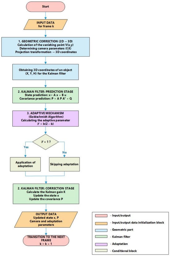
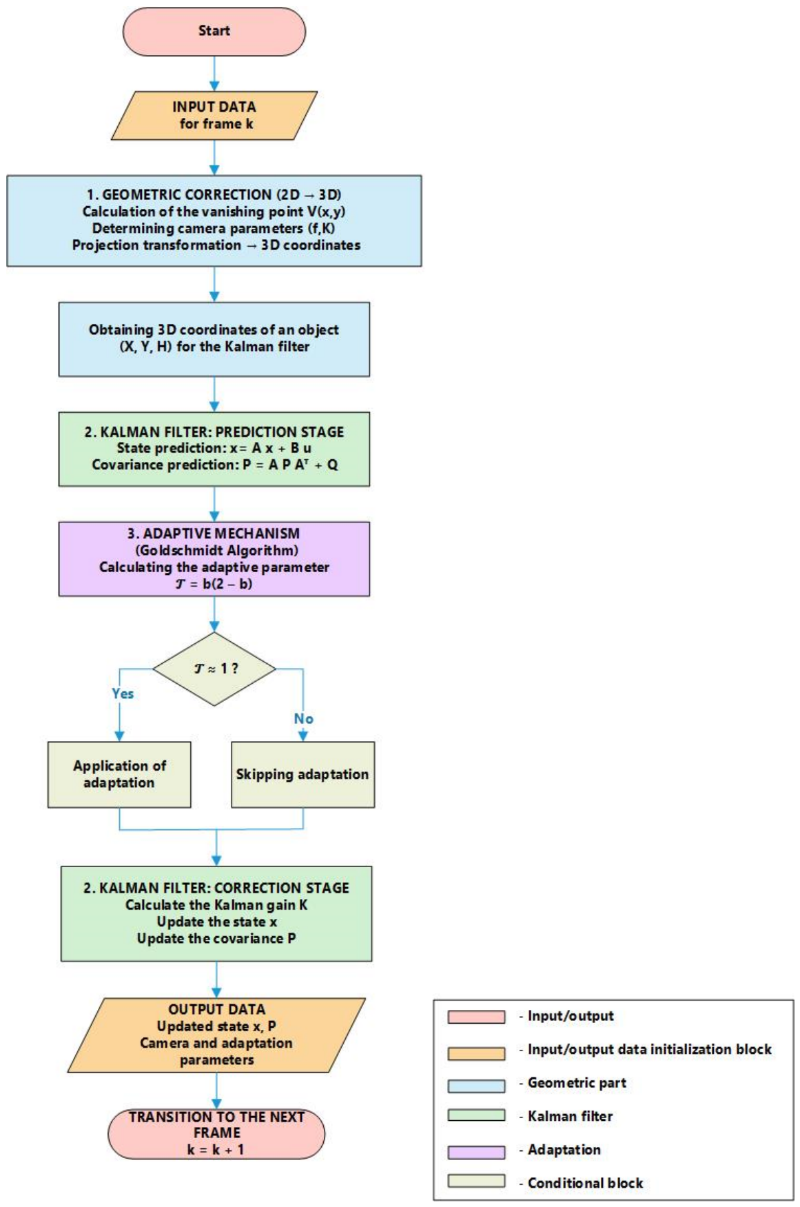
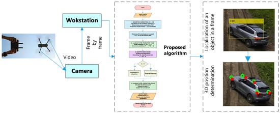
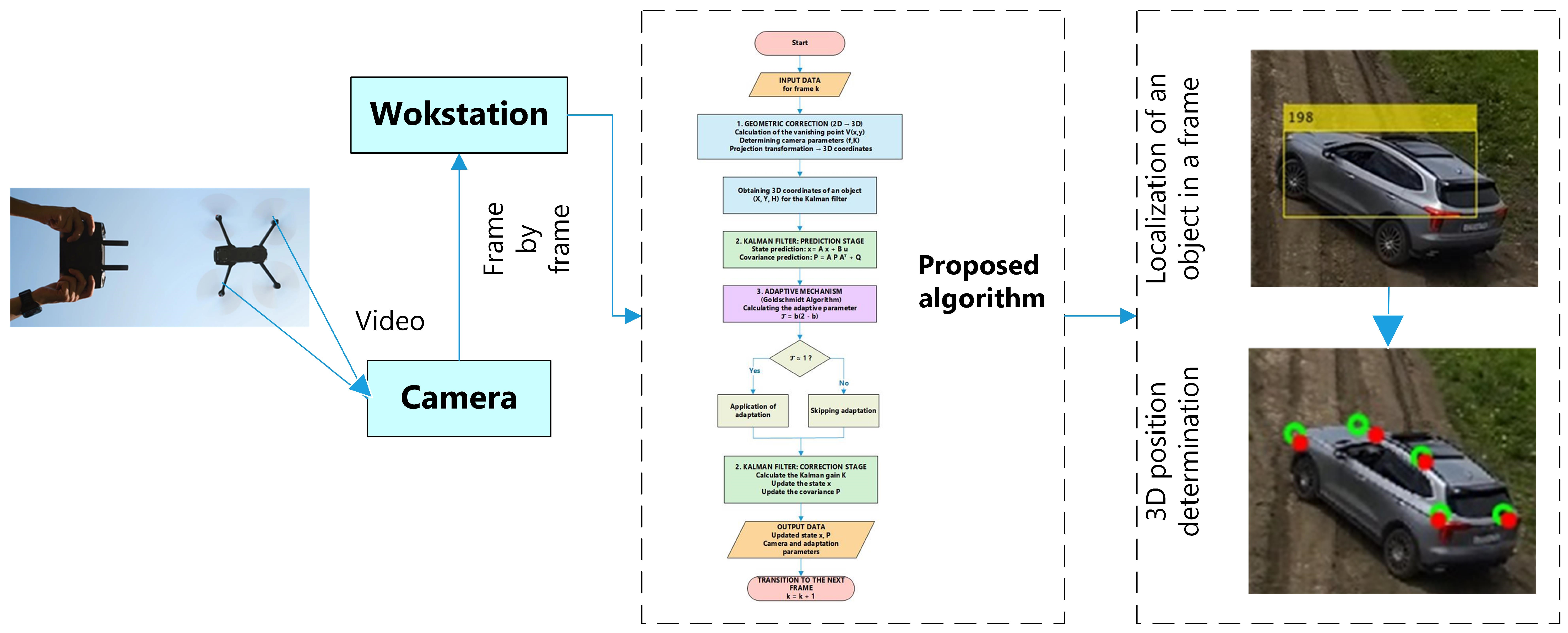
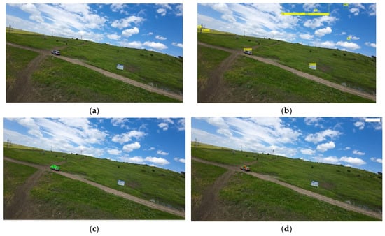
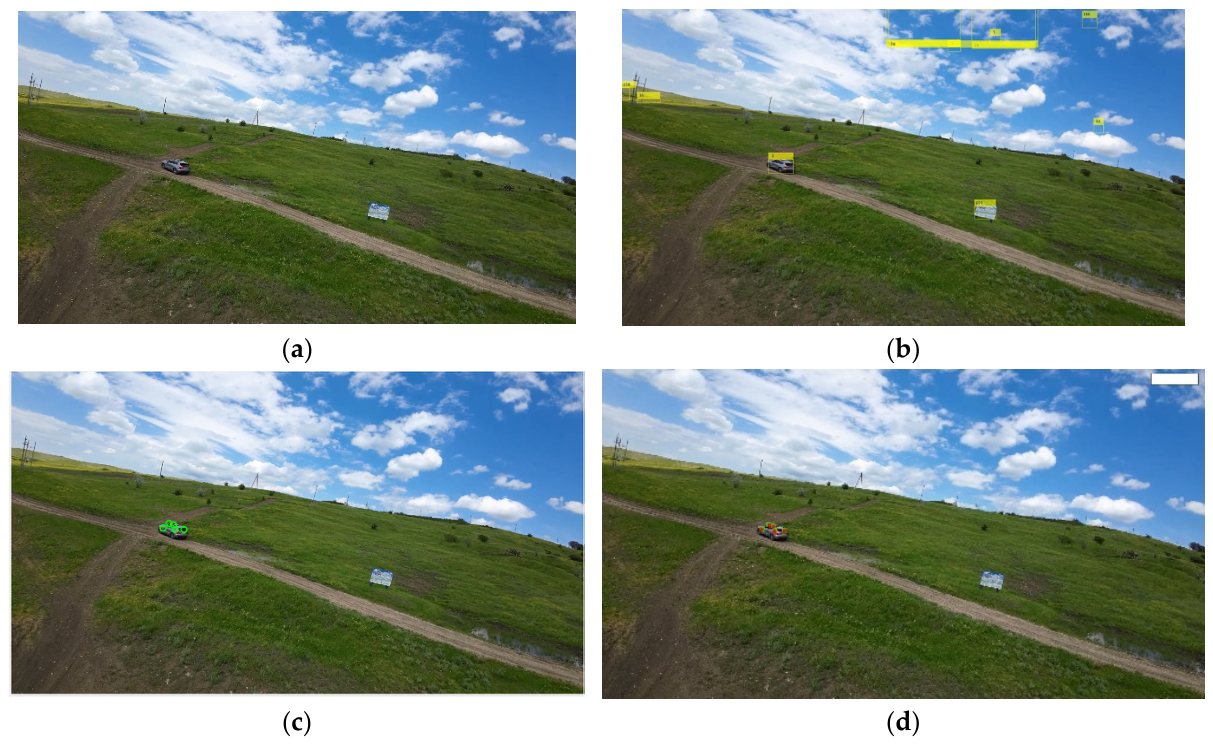
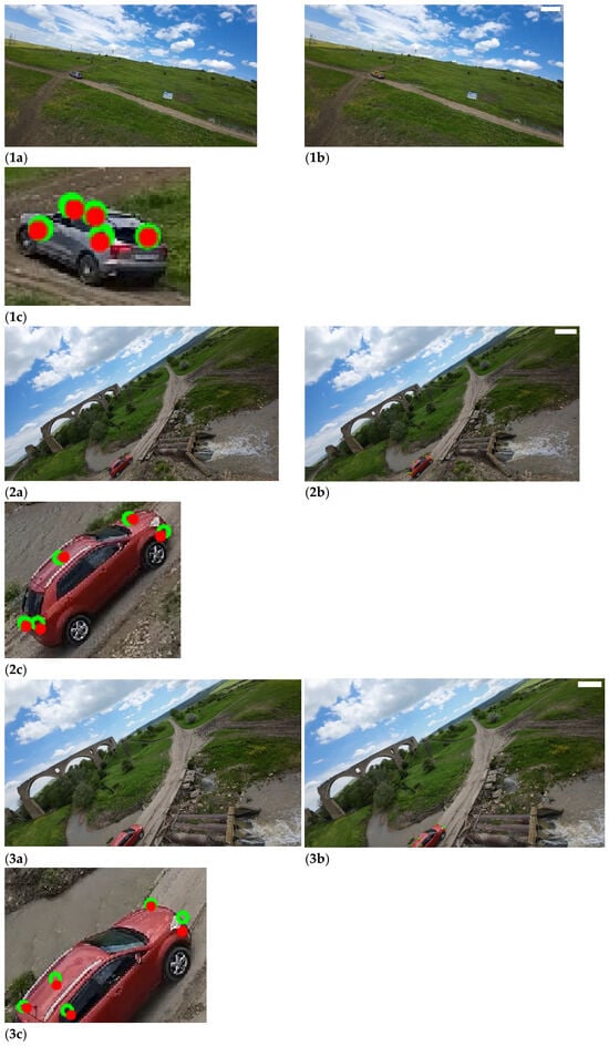
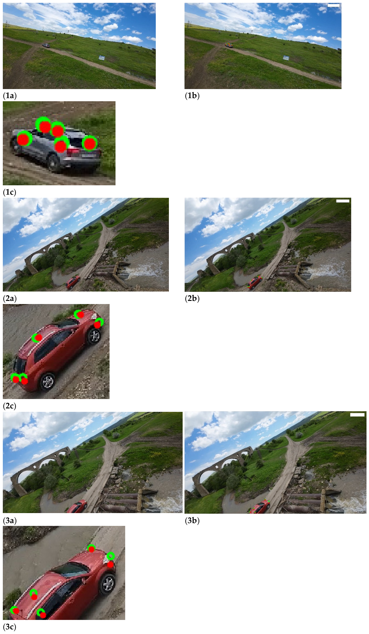
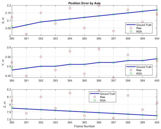
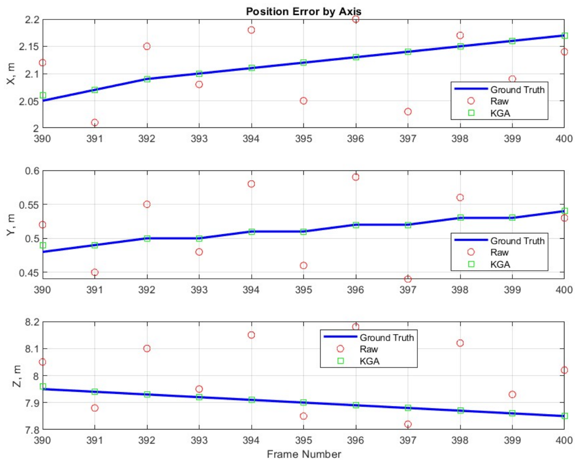
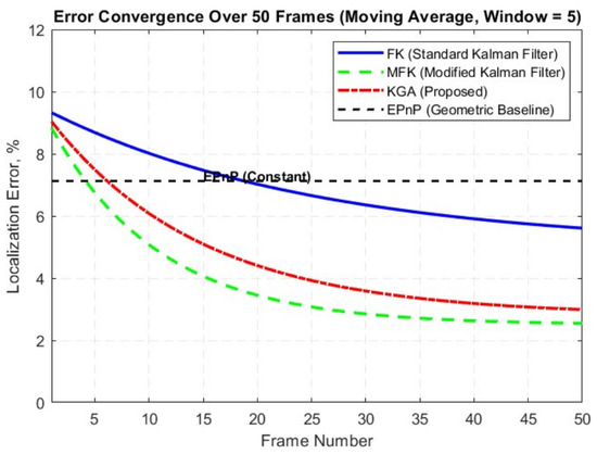
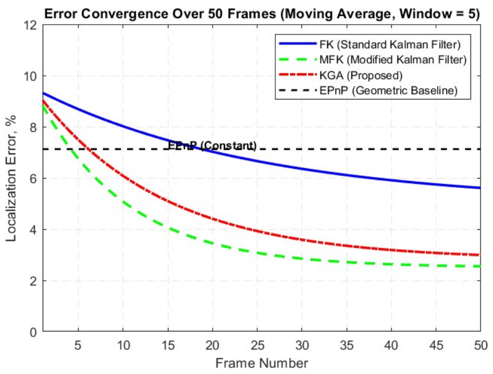
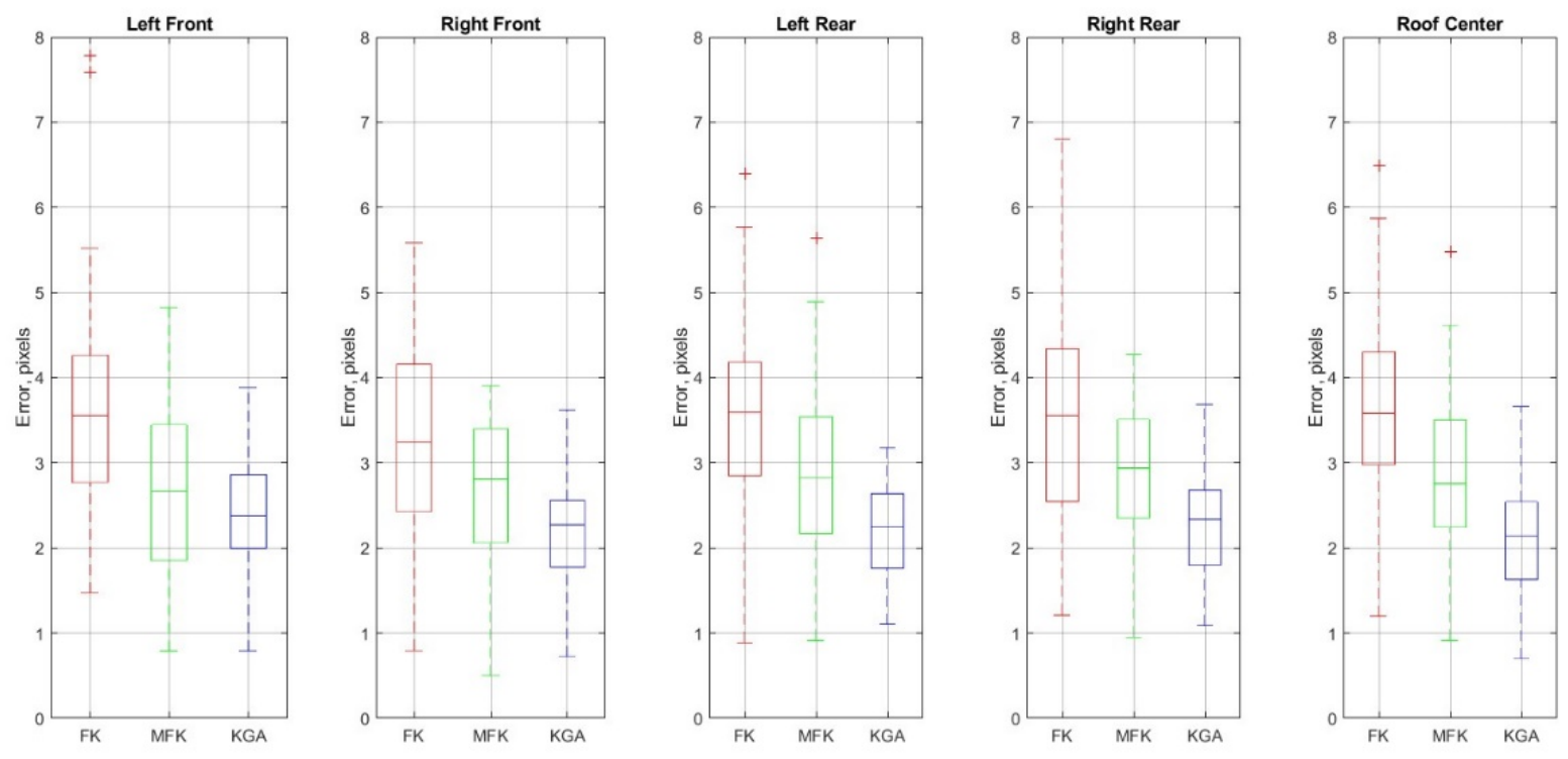
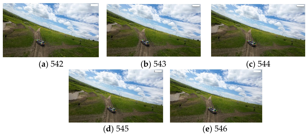
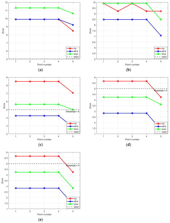
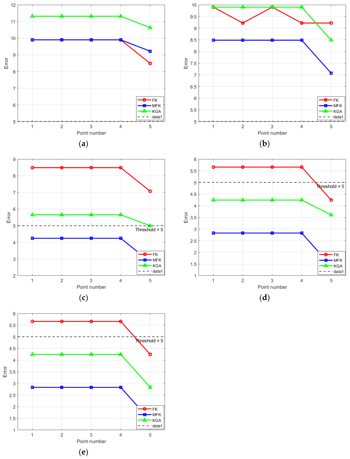
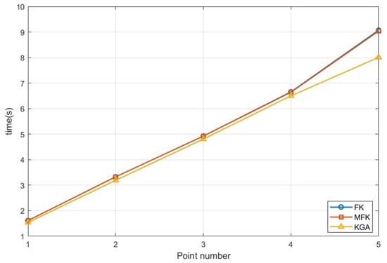
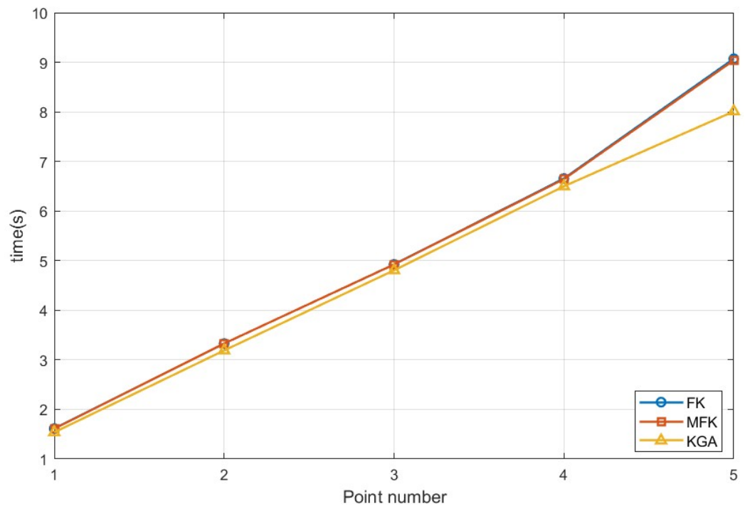

Disclaimer/Publisher’s Note: The statements, opinions and data contained in all publications are solely those of the individual author(s) and contributor(s) and not of MDPI and/or the editor(s). MDPI and/or the editor(s) disclaim responsibility for any injury to people or property resulting from any ideas, methods, instructions or products referred to in the content. |
© 2026 by the authors. Licensee MDPI, Basel, Switzerland. This article is an open access article distributed under the terms and conditions of the Creative Commons Attribution (CC BY) license.