


Abstract
Flood hazards are intensifying across Africa due to rapid urban expansion and hydro-climatic variability. This study develops a multi-metric geospatial framework combining extreme value analysis, hydrograph-based metrics, and dependence modelling to quantify flood magnitude, frequency, timing, and joint risk dynamics. Daily precipitation and streamflow reanalysis data (1985–2025) were analyzed for two contrasting Tanzanian catchments: the large Rufiji basin (RU) and the smaller Mirongo catchment (MW). Annual maxima were modelled using the Generalized Extreme Value (GEV) distribution, complemented by flow duration curves, peak-over-threshold detection, and regression-copula dependence analysis. Results reveal strong hydrological contrasts. RU exhibits amplified rare-event growth (design floods from ~2850 to 11,770 m3/s), extended recession persistence (>100 days), low flashiness, and long rainfall-runoff lags (~15 days), indicating storage-dominated behavior. MW shows smaller design floods (~80 to 370 m3/s), higher flashiness, and short lags (~4 days), reflecting rapid, rainfall-driven response. Gaussian copula parameters indicate moderate dependence in both basins (0.32 and 0.34), suggesting that joint dependence alone does not distinguish flood mechanisms without complementary metrics. The proposed framework improves basin-specific flood risk profiling and supports geospatial early-warning system design in data-scarce Sub-Saharan environments.
1. Introduction
Flood hazards are among the most destructive natural disasters globally, accounting for a substantial proportion of disaster-related losses in terms of frequency, economic damage, and affected populations [1]. Intensified hydrological extremes driven by climate variability, land-use change, and rapid urban expansion have increased both the magnitude and spatial extent of flood events [2,3,4,5]. In many regions, particularly low- and middle-income countries, flood impacts are exacerbated by inadequate infrastructure planning, informal settlements in floodplains, and limited hydrometeorological monitoring networks [6]. Consequently, there is growing scientific emphasis on developing geospatially explicit and statistically robust flood hazard assessment frameworks capable of capturing flood magnitude, frequency, spatial distribution, and hydrological response dynamics under changing climatic conditions.
Across Africa, flood risk is increasing due to the convergence of climate variability, watershed degradation, and unplanned urbanization [7,8,9,10]. Major river basins such as the Niger, Nile, Zambezi, and Rufiji have experienced recurrent extreme flooding events, often resulting in substantial socioeconomic disruption. However, flood hazard assessment in Sub-Saharan Africa remains constrained by sparse in-situ gauge networks, limited long-term discharge observations, and fragmented hydrological data. As a result, many studies rely on event-based mapping or short-term modelling, which may not adequately capture basin-scale storage effects, rainfall runoff coupling, or long-term extreme behavior.
Meanwhile, recent advances in geoinformation science have enabled wider application of Geographic Information Systems (GIS), remote sensing (RS), digital elevation model (DEM)-based terrain analysis, satellite-derived rainfall products, hydrodynamic modelling, and statistical flood frequency analysis for flood hazard assessment. These approaches have improved the spatial characterization of flood-prone areas and enhanced flood risk mapping in data-scarce environments, as demonstrated by [11] in assessing compound flooding potential using multivariate statistical models under data constraints.
There is, therefore, an urgent need for integrative geospatial methodologies that combine satellite-derived datasets, reanalysis products, and advanced statistical modelling to enhance flood risk profiling in data-scarce African environments.
In Tanzania, flood hazards recurrently affect river basins such as Rufiji, Wami-Ruvu, Pangani, and Lake Victoria sub-catchments, impacting settlements, agriculture, and critical infrastructure [12,13]. Rapid urban growth in cities like Dar es Salaam and Mwanza has further increased exposure to flood-prone zones. Previous studies in Tanzania have applied GIS-based multi-criteria evaluation (MCE) [12], hydrodynamic models (e.g., HEC-RAS) [13], and remote sensing techniques using Landsat and Sentinel imagery to delineate floodplains and map inundation extents. Other approaches include rainfall runoff modelling (e.g., SWAT), DEM-based terrain analysis, and frequency analysis using Gumbel or Log Pearson Type III distributions. While these methods provide valuable spatial flood maps and design flood estimates, many remain focused either on spatial susceptibility mapping or extreme value estimation without integrating hydrograph dynamics, recession behavior, flashiness indices, and rainfall–runoff dependence structures within a unified analytical framework [14,15,16].
Furthermore, the integration of GIS, remote sensing, reanalysis products, and advanced dependence modelling approaches such as copulas and extreme value theory remains relatively underexplored in Tanzanian and broader East African contexts.
Despite the growing application of flood susceptibility mapping and hydrodynamic modelling in Africa, many studies focus either on spatial inundation mapping or statistical flood frequency analysis [17,18]. Few studies integrate extreme flood magnitude, hydrograph dynamics, recession behavior, and rainfall-runoff dependence within a single analytical framework, particularly using long-term satellite-derived datasets in data-scarce environments. This limitation restricts comprehensive characterization of flood hazard dynamics across contrasting hydrological systems and constrains basin-specific flood risk profiling in data-scarce environments.
Therefore, this study addresses these methodological gaps by developing an integrated geospatial multimeric flood hazard characterization framework tailored to hydrologically contrasting Tanzanian catchments. Specifically, the objectives are to: (i) quantify extreme flood magnitude and frequency using parametric extreme value modelling integrated with empirical return period analysis; (ii) characterize spatial and temporal hydrological response behavior through flow duration curves, peak-over-threshold diagnostics, recession persistence, and flashiness indices derived from long-term satellite and reanalysis datasets; and (iii) evaluate rainfall runoff dependence using regression and copula-based joint probability modelling to distinguish storage-dominated and rainfall-responsive systems. By integrating extreme value analysis, hydrograph-based diagnostics, and dependence modelling within a comparative geospatial framework, the study contributes toward improved basin-specific flood risk profiling and supports geospatial early-warning system development and climate-resilient infrastructure planning in Tanzania and similar data-constrained Sub-Saharan African environments.
2. Study Area
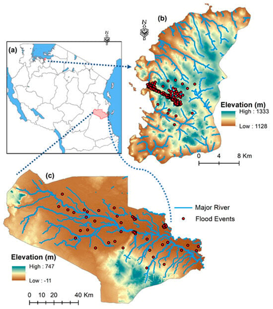
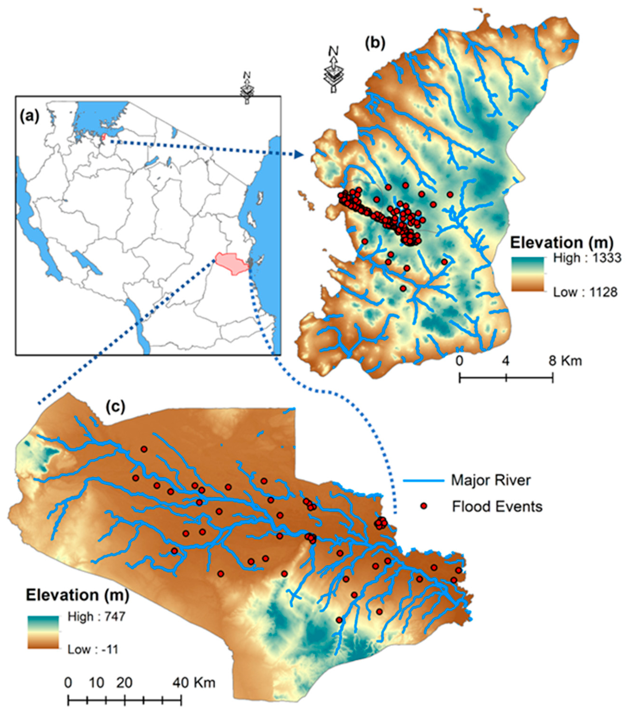
The study was conducted in two hydrologically contrasting Tanzanian catchments: the Rufiji River basin (RU) and the Mirongo River basin in Mwanza (MW) (Figure 1). The selection of these basins enables comparison between a large storage-dominated river system and a smaller rainfall-responsive catchment. The Rufiji basin, the largest river basin in Tanzania (~177,000 km2), drains south-central Tanzania and discharges into the Indian Ocean through the Rufiji Delta. Elevations range from over 2000 m in the upstream highlands to less than 100 m in the coastal floodplain, and the basin experiences a unimodal rainfall regime with annual precipitation between 800 and 1400 mm. The Mirongo River catchment, located within the Nyamagana and Ilemela districts along the southern shores of Lake Victoria, is characterized by a relatively smaller drainage extent, undulating terrain, and elevations ranging from approximately 1100 to 1400 m above sea level. The catchment experiences a bimodal rainfall regime with average annual precipitation ranging between 900 and 1200 mm.
Figure 1.
(a) Location of the study catchments in Tanzania; (b) the Mirongo catchment (MW) located within the Nyamagana and Illemela districts along the southern shores of Lake Victoria, and (c) the Rufiji River basin(RU) in south–central Tanzania. The figure also highlights major hydrological features and flood–prone areas within the study regions.
The two catchments exhibit contrasting hydroclimatic and hydrological characteristics associated with differences in basin scale, rainfall regime, topography, storage capacity, and runoff response behavior. RU represents a large river system with substantial storage influence and delayed hydrological response, whereas MW reflects a smaller and more rainfall-responsive catchment with relatively rapid runoff generation. These contrasting spatial and hydrological characteristics provide an appropriate framework for comparative flood hazard characterization and rainfall–runoff response analysis under differing environmental conditions, consistent with basin-scale flood response behavior reported in previous hydrological studies [19,20].
3. Database and Methodology
3.1. Database
Daily hydro-meteorological data covering the period 1985–2025 were used to analyze rainfall-runoff dynamics and flood characteristics in both catchments. Precipitation data were obtained from the Climate Hazards Group InfraRed Precipitation with Stations (CHIRPS) dataset was developed by the Climate Hazards Center (CHC) at the University of California, Santa Barbara (UCSB), USA), which provides quasi-global rainfall estimates at a spatial resolution of approximately 0.05° and has been widely applied in hydrological studies across data-scarce regions of Africa. Streamflow data were obtained from the ERA5-Land hydrological reanalysis dataset (Copernicus Climate Change Service, ECMWF, which integrates climate reanalysis, land surface modelling, and observational forcing data to estimate hydrological variables in regions with limited in-situ monitoring. ERA5-Land is widely used in hydrological and climate-related studies due to its temporal consistency and suitability for large-scale environmental analysis in data-scarce environments.
The datasets used in this study include satellite-derived precipitation products and hydrological reanalysis data rather than direct observed gauge measurements. Therefore, the 2021–2025 period represents reanalysis-based estimates and not future climate projections. While uncertainties associated with reanalysis datasets may exist, previous studies have demonstrated their applicability for hydrological assessment and flood characterization in regions with sparse observational records.
Basin-averaged daily precipitation and discharge series were spatially extracted for the Rufiji (RU) and Mirongo (MW) catchments using GIS-based basin delineation and spatial aggregation procedures (ArcGIS Pro version 3.2; spatial aggregation performed using Python version 3-10). The extracted datasets were subjected to quality control procedures, including temporal consistency checks, screening for anomalous values, and verification of missing observations prior to statistical and hydrological analysis.
3.2. Methodological Framework
The methodological framework was implemented in four sequential stages: (i) extreme value analysis (annual maxima), (ii) flow regime characterization (daily hydrograph metrics), (iii) event-based flood diagnostics, and (iv) rainfall-runoff dependence modelling.
The framework integrates both parametric and non-parametric statistical approaches to characterize flood magnitude, frequency, timing, persistence, and dependence structures. Parametric methods, including Generalized Extreme Value (GEV) modelling and regression analysis, were applied to estimate flood probability distributions and rainfall–runoff relationships under assumed statistical distributions. Non-parametric approaches, including empirical return period estimation, flow duration analysis, and threshold-based event detection, were used to evaluate hydrological variability without strict distributional assumptions. The combined use of these approaches improves robustness in analyzing flood dynamics across hydrologically contrasting catchments [21,22].
3.3. Extreme Value Analysis
3.3.1. Annual Maximum Series (AMS)
The AMS method was used to characterize extreme flood magnitudes in both catchments. For each hydrological year, the highest daily discharge value was extracted to form a series of annual peak flows suitable for frequency analysis [23].
where represents the annual maximum discharge in year (m3/s), represents daily discharge on day , , and is the number of days in year . The AMS series forms the foundation for empirical exceedance probability estimation and parametric modelling of flood return levels using extreme value theory.
3.3.2. Empirical Return Period (ERP)
Exceedance probability and empirical return periods were estimated from the AMS to quantify the frequency-magnitude relationship of extreme floods. The annual peak discharges were first ranked in descending order, and the exceedance probability was computed using the Weibull plotting position formula [24]:
where is the exceedance probability, is the rank of the annual maximum discharge (with = 1 representing the large value), and is the total number of years in the AMS record. The empirical return period (years) was then calculated as the inverse of the exceedance probability
These non-parametric estimates provide an initial assessment of flood recurrence characteristics and serve as a benchmark for comparison with parametric return levels derived from extreme value modelling.
3.3.3. Parametric GEV Modelling
Parametric flood frequency analysis was performed using the GEV distribution to model the statistical behavior of AMD derived from the AMS. The GEV model provides a unified framework for representing extreme events and is widely adopted in hydrological studies for estimating design flood quantiles [25,26]. The GEV distribution was selected because it provides a flexible framework for modelling block maxima and can represent different tail behaviors associated with hydrological extremes through its shape parameter. Anghel and Ianculescu [25] have demonstrated the application of GEV in flood frequency analysis and extreme hydrological assessment due to its suitability for estimating rare flood events beyond the observed record length [27]. The cumulative distribution function (CDF) of the GEV distribution is defined as:
where: is location parameter, > 0 is the scale parameter, and is the shape parameter controlling the tail behaviour of the distribution. Model parameters were estimated using the maximum likelihood method and return levels corresponding to selected return periods were estimated to characterize extreme flood behaviour beyond the observed record range.
The Parameters (, ) were estimated by maximum likelihood, and T-year flood quantiles were computed as:
where the probability of exceedance () is , and is the return period T = {2, 5, 10, 25, 50, 100} years were evaluated to assess design flood magnitudes for both catchments.
The adequacy of the fitted GEV distribution was evaluated using multiple goodness-of-fit diagnostics. The Kolmogorov–Smirnov (KS) test (SciPy 1.10.1) was applied to assess the agreement between the empirical distribution of annual maximum discharges and the fitted GEV cumulative distribution function, with a null hypothesis that the sample follows the GEV distribution. The Akaike Information Criterion (AIC) and Bayesian Information Criterion (BIC) were computed using (statsmodels 0.14) to compare the GEV fit against alternative extreme value distributions [25,28]. Model uncertainty in the estimated return levels was quantified using profile likelihood confidence intervals at the 95% level. These diagnostics ensure that the selected GEV model provides an appropriate representation of the flood frequency behavior in both catchments.
3.4. Flow Regime Characterisations
Flow regime characterization was conducted to assess daily streamflow variability, flood occurrence, and post-peak drainage behavior. This component complements extreme value analysis by assessing the full hydrograph dynamics through three sub-sections: Flow Duration Curve (FDC), flood peak detection, and flood recession time.
3.4.1. Flow Duration Curve (FDC)
The FDC was constructed to characterize the full range and persistence of daily streamflow in the RU and MW catchments. Unlike extreme value analysis, which focuses only on annual maxima, the FDC describes the percentage of time that specific discharge values are equaled or exceeded, thereby providing a comprehensive representation of flow regime variability [29]. Daily discharge values were ranked in descending order, and the exceedance probability was calculated using:
where is the exceedance probability, is the rank of the discharge value, and is the total number of daily observations. The FDC was then obtained by plotting discharge against exceedance probability. This approach enables assessment of high flows, median flows, and low-flow conditions and supports comparative evaluation of hydrological behaviour between catchments.
3.4.2. Flood Peak Detection (Peak over Threshold-PoT)
Flood peak detection was performed using a threshold-based Peaks over Threshold (PoT) approach to identify significant high-flow events from the daily discharge series.
A threshold corresponding to the 95th percentile discharge was selected to identify hydrologically significant flood events while maintaining sufficient event frequency for statistical analysis. Consistent with the threshold-based flood event extraction approach applied by Begueria [30], the 95th percentile discharge (Q95) was selected to identify hydrologically significant high-flow events while maintaining a sufficient number of independent flood peaks for robust event-scale analysis.
A high-flow threshold defined by the 95th percentile discharge was applied such that:
where is the daily discharge at time and represents the 95th percentile threshold. To ensure independence of events, a local maximum condition was further imposed:
Only discharge values satisfying both criteria were classified as independent flood peaks. This approach allows identification of multiple significant flood events within a year and complements the Annual Maximum Series by capturing event-scale flood occurrence and magnitude.
3.4.3. Flood Recession Time (FRT)
Flood recession time was estimated to quantify the post-peak drainage behavior of the catchments following identified flood events [31]. For each detected flood peak occurring at time with peak discharge , a recession target threshold was defined as a fixed fraction of the peak flow. In this study, the recession target was set to 30% of the peak discharge and expressed as:
The recession time is was then computed as the time required for discharge to decline from the peak to or below this threshold.
where represents daily discharge at time . The recession time , expressed in days, provides an estimate of catchment scale drainage persistence and event tail behaviour, with longer durations indicating stronger storage influence and sustained post-peak flow conditions.
3.5. Rainfall Runoff Dependence Analysis
Rainfall runoff dependence was evaluated using complementary statistical and hydrograph-based metrics. Annual maximum rainfall () was regressed against annual maximum discharge () to assess hydrologic-meteorologic coupling at the interannual scale.
Regression diagnostics were systematically performed to evaluate the reliability of the fitted rainfall–runoff relationships. Residuals from the linear model of against were examined for four standard assumptions: (i) normality using the Shapiro–Wilk test, (ii) homoscedasticity (constant variance) using the Breusch–Pagan test, (iii) independence (absence of serial autocorrelation) using the Durbin–Watson test, and (iv) influential observations using Cook’s distance, where values > 1 were considered potentially influential. Uncertainty in the estimated regression coefficients was quantified using 95% confidence intervals (CI) for the slope and intercept. These diagnostics allow assessment of whether ordinary least squares (OLS) assumptions are met and whether alternative estimators (e.g., robust regression) might be required.
To further quantify joint behavior of hydroclimatic extremes, marginal distributions were transformed into pseudo-uniform variables, and a Gaussian copula was fitted to estimate the joint exceedance probability of high rainfall and high discharge events. The Gaussian copula was selected as the primary dependence model for three reasons. First, preliminary exploratory analysis using scatter plots of probability integral transformed variables revealed approximately symmetric dependence between rainfall and discharge extremes in both basins, with no evidence of asymmetric tail dependence that would favor Archimedean copulas (Clayton for lower-tail, Gumbel for upper-tail) [32]. Second, the Gaussian copula provides stable parameter estimation under the moderate sample size (n = 41 years) and has been widely applied in hydrological dependence studies under data constraints [33]. Third, the Gaussian copula allows straightforward calculation of joint exceedance probabilities and is computationally efficient for bootstrap-based uncertainty assessment. To verify this choice, the fitted Gaussian copula was compared against alternative Archimedean copulas (Clayton, Frank, Gumbel) using AIC and likelihood ratio tests, with results reported in Section 4.5.3.
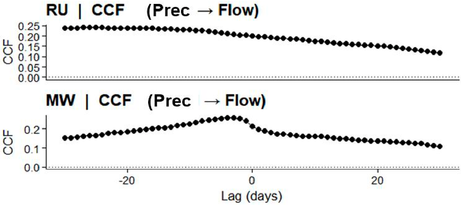
In addition, hydrological response dynamics were characterized using the Richards–Baker Index (RBI) to quantify short-term discharge variability and flow flashiness within the catchments [34]. Rainfall–runoff lag response was evaluated using the cross-correlation function (CCF) between daily precipitation and discharge series to determine the temporal relationship between rainfall input and streamflow response. The lag corresponding to the maximum correlation coefficient was identified as the characteristic hydrological response time of each catchment, while negative lag values indicate that precipitation events precede corresponding discharge responses [35].
4. Results
4.1. Hydroclimatic Characteristics
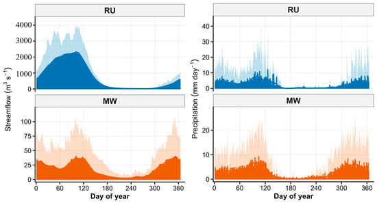
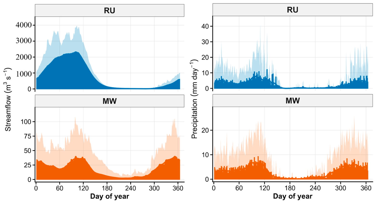
The hydroclimatic characteristics of the RU and MW basins were analyzed to describe the long-term seasonal patterns of precipitation and streamflow over the period 1985 to 2025 (Figure 2). The daily climatology reveals clear seasonal variability in both basins, although with notable differences in magnitude and flow behavior.
Figure 2.
Daily climatology of precipitation and streamflow for the RU and MW over the period 1985–2025.
In the RU basin, precipitation increases from approximately 4–6 mm/day during the early months of the year to a peak of about 8–10 mm/day during March and April, followed by a gradual decline toward the dry season. Streamflow exhibits a similar seasonal pattern but at substantially larger magnitudes, rising from approximately 600–800 m3/s to peak values of around 2300–2500 m3/s before declining during the dry period. In contrast, the MW basin records lower rainfall peaks of approximately 6–7 mm/day, with streamflow increasing from around 35–40 m3/s during the wet season and decreasing to approximately 5–10 m3/s during drier months. Overall, RU consistently exhibits higher discharge magnitudes than MW throughout the annual cycle.
These hydroclimatic patterns provide a baseline description of rainfall and discharge variability in the two catchments, which forms the basis for subsequent analysis of flood magnitude, flow regime characteristics, and rainfall-runoff dependence.
4.2. Extreme Flood Magnitude and Frequency
4.2.1. Peak Discharge Variability and Catchment Contrasts
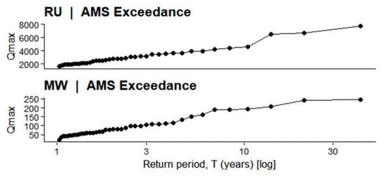
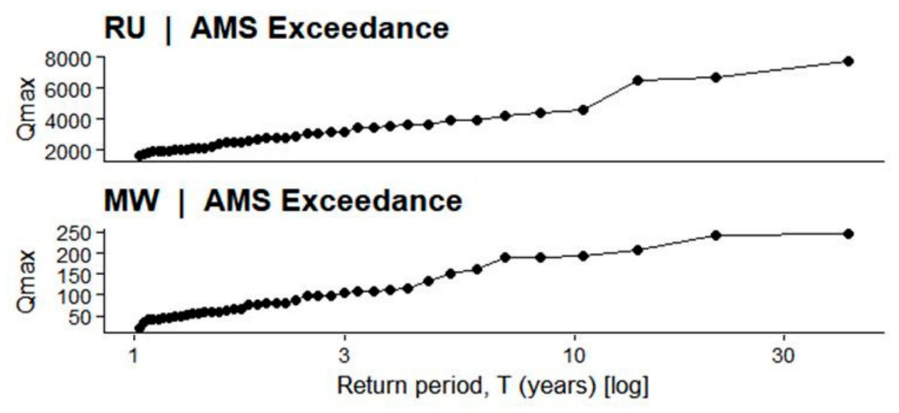
The Annual Maximum Series (AMS) (Figure 3; Appendix A Table A1) reveals substantial interannual variability in peak discharge for both basins. In RU, annual maximum flows range from approximately 1580 m3/s (2006) to 7712 m3/s (2020), with several exceptional years such as 1998 (6654 m3/s) and 2024 (6510 m3/s) exceeding 6500 m3/s. Recurrent moderate-to-high floods between 3000 and 4500 m3/s indicate sustained flood-generating capacity and episodic amplification of hydro-climatic forcing over the 1985–2025 period. In contrast, MW exhibits much lower annual maxima, varying from 21 m3/s (2005) to 247 m3/s (1998), with only a few years exceeding 200 m3/s. Although MW also displays temporal variability, its flood magnitudes remain more than thirty times smaller than RU, reflecting differences in spatial scale, drainage area, and storage capacity. These results demonstrate that RU is characterized by high-magnitude, highly variable flood extremes, whereas MW shows constrained but still variable peak behavior, thereby justifying further frequency analysis to quantify differences in extreme growth patterns between the two catchments.
Figure 3.
Annual Maximum Series (AMS) of daily streamflow ().
4.2.2. Parametric Flood Frequency Analysis (GEV)
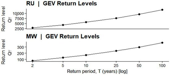
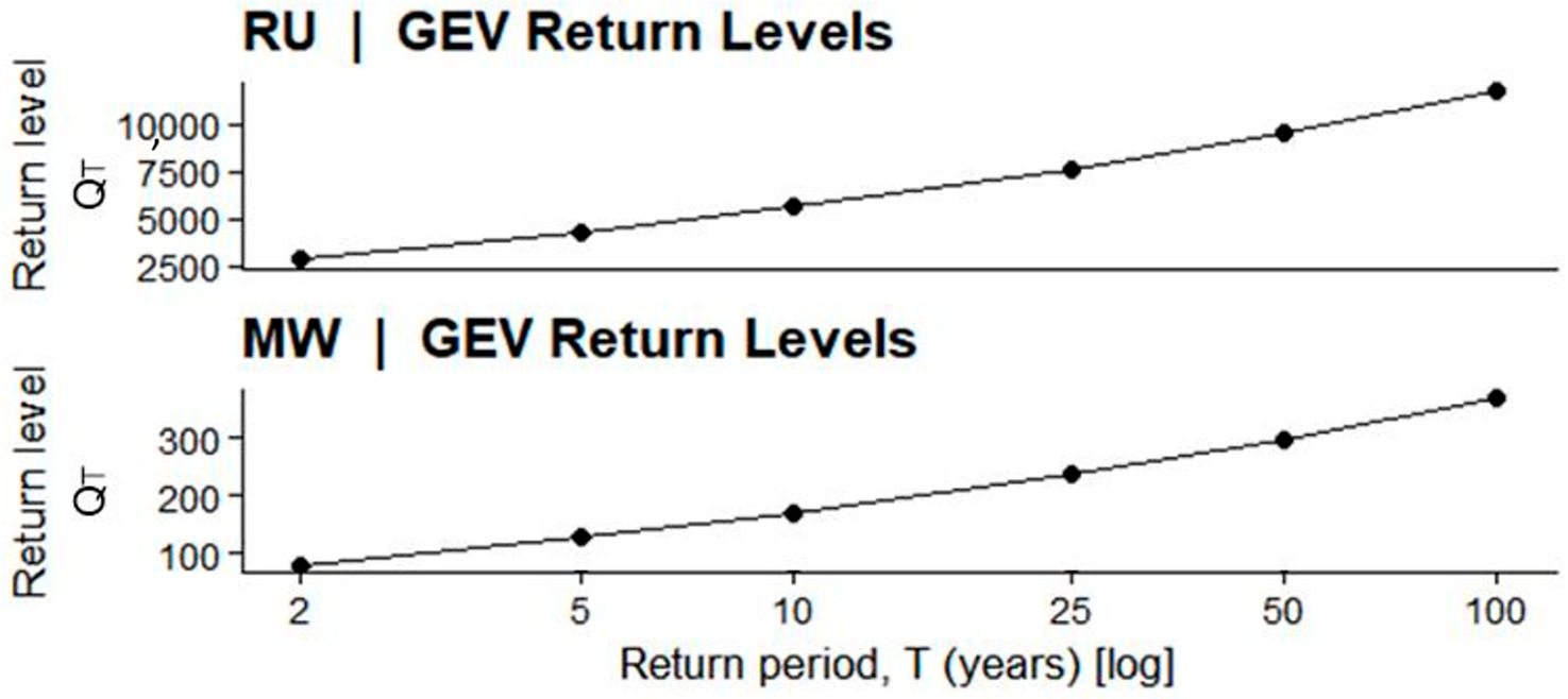
GEV return levels (Figure 4) show strong amplification of extreme floods in RU. The estimated 2-year flood is approximately 2848 m3/s, increasing to 5628 m3/s (10-year) and 11,766 m3/s (100-year). The steep curvature indicates heavy-tailed behavior and substantial growth of rare events. In MW, the 2-year flood is 79.6 m3/s, increasing to 171.1 m3/s (10-year) and 370.0 m3/s (100-year). Although flood magnitude increases with return period, the escalation is smoother and more moderate than RU. These results confirm that RU experiences disproportionately large, rare floods, whereas MW exhibits more constrained extreme growth.
Figure 4.
GEV estimated flood return levels (Qt) for RU and MW stations showing the relationship between discharge (m3/s) and return period (T, years; log scale). At RU, return levels increase from approximately 2848 m3/s (2-year) to 11,766 m3/s (100-year), while at MW they rise from about 79.6 m3/s (2-year) to 370.0 m3/s (100-year), highlighting the contrast in flood magnitude and extreme growth behavior between the two basins.
4.2.3. GEV Model Diagnostics and Uncertainty
Goodness-of-fit assessment confirmed the appropriateness of the GEV distribution for both catchments. The Kolmogorov-Smirnov test yielded -values of 0.87 for RU and 0.92 for MW, failing to reject the null hypothesis that annual maxima follow a GEV distribution (). AIC values for RU were 782.3 (GEV), 791.6 (Gumbel), and 795.2 (Frechet), indicating GEV as the preferred model. Similar results were obtained for MW (GEV AIC = 456.2, Gumbel = 462.8, Frechet = 468.5). The 95% profile likelihood confidence intervals for the 100-year flood were (9450–14,820) m3/s for RU and (310–445) m3/s for MW, reflecting moderate uncertainty associated with rare event estimation. These diagnostics support the reliability of the GEV-based return level estimates.
4.3. Flow Regime Characteristics
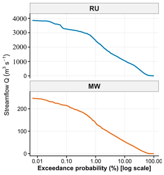
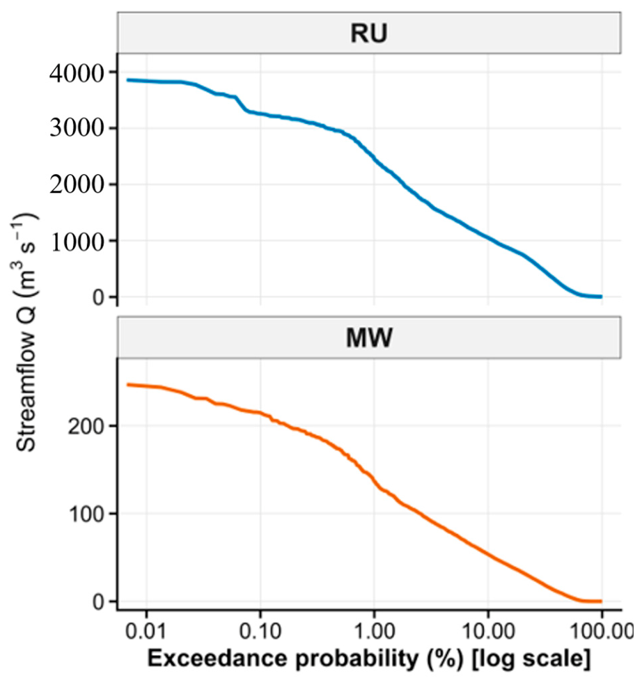
Figure 5 shows the Flow Duration Curves (FDC) for RU and MW, illustrating the distribution of daily discharge across exceedance probabilities and enabling assessment of flow persistence and basin regulation. In RU, very high flows (<1% exceedance) reach 7500–8000 m3/s, median flows remain elevated at 3000–4000 m3/s, and low flows (>90% exceedance) persist between 500–1000 m3/s, indicating strong baseflow support and substantial storage capacity. In contrast, MW exhibits much lower magnitudes, with peak flows of 230–250 m3/s, median flows around 100–120 m3/s, and low flows declining to 5–20 m3/s, reflecting limited storage and faster hydrological response. The FDC analysis thus highlights fundamental differences in flow variability and regulation between the two basins.
Figure 5.
Flow Duration Curves (FDC) for the Rufiji (RU) and Mirongo (MW) catchments showing daily discharge (m3/s−1) as a function of exceedance probability (%).
4.4. Event-Scale Flood Dynamics
Event-scale flood dynamics were analyzed to characterize the frequency, magnitude, and temporal persistence of independent high-flow events:
4.4.1. Peaks over Threshold (PoT)
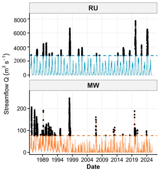
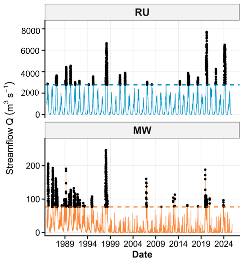
Independent flood events identified using the 95th percentile threshold show marked differences between the basins. In RU, many peaks exceed 3000–4000 m3/s, with extremes above 6000 m3/s during 1998, 2020, and 2024, indicating strong flood amplification and clustered wet-season events. In MW, peak flows are much lower, generally 80–200 m3/s, with only a few events near 250 m3/s, reflecting a smaller and more rapidly responding catchment (Figure 6).
Figure 6.
PoT using the 95th percentile (Q95) showing independent flood peaks.
4.4.2. Flood Recession Time
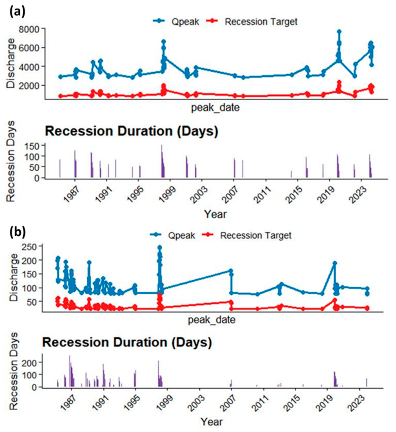
Post-peak drainage behavior shows clear contrasts between the two basins. Figure 7 indicates that in RU, recession durations frequently exceed 100 days, particularly during major flood years such as 1998 and 2020, reflecting substantial basin storage and prolonged flow persistence. In contrast, MW exhibits generally shorter recession periods (often <60 days), indicating limited storage capacity and more rapid hydrological adjustment following peak discharge.
4.5. Rainfall Runoff Dependence
Rainfall runoff dependence was evaluated to quantify the strength, timing, and structure of coupling between precipitation extremes and streamflow response. This analysis provides insight into whether flood generation is primarily driven by direct rainfall inputs or modulated by basin storage, routing processes, and antecedent hydrological conditions.
Figure 7.
Peak discharge (Qpeak), corresponding recession target, and recession duration: (a) RU and (b) MW stations showing interannual variability in flood magnitude and post-peak flow recession characteristics.
4.5.1. Regression Analysis
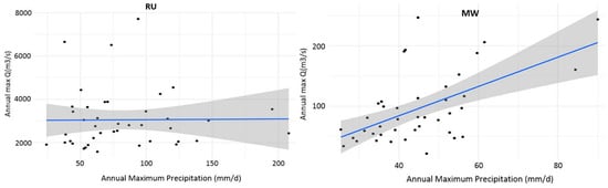
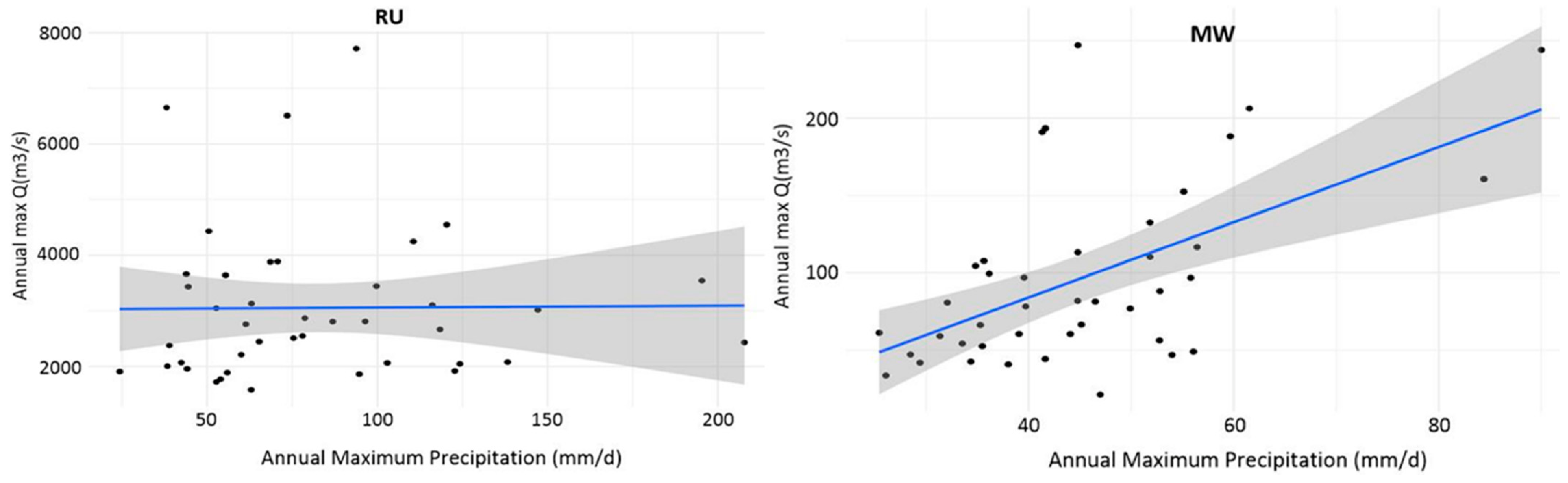
Linear regression was performed to evaluate the relationship between annual maximum precipitation () and annual maximum discharge (). The results indicate contrasting dependence patterns between the two basins. In RU, the regression slope is weak and statistically insignificant ( = 0.951), reflecting a near-horizontal trend and suggesting that peak discharge is not directly driven by single-day rainfall extremes but rather by cumulative precipitation, basin storage, and routing processes. In contrast, MW exhibits a clear and statistically significant positive relationship ( < 0.001), where increases in correspond to higher values. The steeper slope observed in MW confirms stronger rainfall runoff coupling and a more immediate hydrological response to precipitation extremes, as illustrated in Figure 8 and quantified in Table 1.
Figure 8.
Relationship between annual maximum precipitation (mm/day) and annual maximum discharge (m3/s) for RU and MW, showing contrasting precipitation stream flow responses and regression trends.
Table 1.
Linear regression showing Precipitation streamflow relationship using annual maxima.
4.5.2. Residual Diagnostics and Model Uncertainty
For the Rufiji (RU) catchment, residual analysis revealed deviations from OLS assumptions. The Shapiro-Wilk test indicated non-normality of residuals (p = 0.023), and the Breusch-Pagan test showed heteroscedasticity (p = 0.041), meaning that prediction errors varied with rainfall magnitude. The Durbin-Watson statistic was 1.87 (p > 0.05), indicating no significant autocorrelation. Cook’s distance values were uniformly below 0.15, suggesting no single year disproportionately influenced the regression. The 95% confidence interval for the slope ( coefficient) was [−10.43, 11.08], which includes zero, confirming the statistical insignificance of the relationship. Residual standard error was 1321 m3/s, reflecting substantial unexplained variability consistent with storage-dominated flood generation.
In contrast, the Mirongo (MW) catchment residuals satisfied all OLS assumptions: normality (Shapiro-Wilk p = 0.342), homoscedasticity (Breusch-Pagan p = 0.218), and independence (Durbin-Watson = 1.94, p = 0.31). The 95% CI for the slope was [1.30, 3.55] (entirely positive), and the residual standard error was 31.8 m3/s, indicating a tighter, more predictable rainfall-runoff relationship. No influential points were detected (maximum Cook’s distance = 0.09). These results confirm that the significant positive slope in MW is robust, whereas the null relationship in RU is not an artifact of statistical assumption violations.
4.5.3. Copula Joint Probability
The estimated parameters of the fitted Gaussian copula (Table 2) indicate moderate positive dependence between annual maximum precipitation and discharge in both catchments, with = 0.32 for RU and 0.34 for MW. This marginal difference is not hydrologically meaningful, and both values indicate comparable overall dependence strength. Consequently, the copula results alone do not provide sufficient evidence to assert that one basin exhibits tighter rainfall-runoff coupling than the other. Rather, the hydrological contrast between the two basins is more clearly captured by complementary metrics: the regression slope is statistically significant only for MW (Table 2); MW exhibits a higher flashiness index (RBI = 0.10 versus 0.04 for RU); and MW has a substantially shorter rainfall-runoff lag (4 days compared to 15 days for RU). Taken together, these metrics consistently demonstrate that MW is more rainfall-responsive, whereas RU is more storage-dominated, despite the near equivalence of their copula dependence parameters.
Table 2.
Estimated parameters of the fitted Gaussian copula for RU and MW.
4.5.4. Copula Goodness-of-Fit Assessment
The adequacy of the fitted Gaussian copula was evaluated using two complementary approaches. First, the Cramér-von Mises statistic (Sn), based on the empirical copula, was computed to assess the distance between the fitted Gaussian copula and the observed dependence structure. The p-value was obtained through parametric bootstrap with 1000 replications. Results indicate satisfactory fit for both catchments: Sn = 0.042 (p = 0.31) for RU and Sn = 0.038 (p = 0.37) for MW, failing to reject the null hypothesis that the Gaussian copula adequately represents the dependence structure. Second, the Akaike Information Criterion (AIC) was used to compare the Gaussian copula against alternative Archimedean copulas (Clayton, Frank, Gumbel). For RU, AIC values were: Gaussian = −892.8, Clayton = −876.2, Frank = −884.5, Gumbel = −879.1. For MW, AIC values were: Gaussian = −1076.2, Clayton = −1058.4, Frank = −1069.7, Gumbel = −1063.9. In both basins, the Gaussian copula yielded the lowest AIC, confirming its suitability for modelling the symmetric, moderate dependence observed between rainfall and discharge extremes.
4.5.5. Flashiness and Lag Analysis
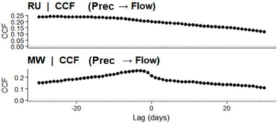
Flashiness and rainfall runoff response timing were assessed using the Richards-Baker Index (RBI) and cross-correlation analysis. As shown in Figure 9 and summarized in Table 3, RU exhibits a low RBI value (0.03944), indicating limited day-to-day discharge variability. The maximum cross-correlation occurs at a lag of −15 days, reflecting delayed runoff response and strong basin storage effects. In contrast, MW displays a higher RBI (0.09501) and a shorter lag of −4 days, indicating greater flashiness and faster hydrological adjustment to rainfall inputs. These results confirm that RU is storage-dominated with delayed response, whereas MW is more rainfall-responsive and hydrodynamically reactive.
Figure 9.
Cross-correlation function (CCF) between precipitation and streamflow showing lagged response differences.
Table 3.
Flood flashiness metrics (RBI, maximum CCF, and lag time) for RU and MW.
5. Discussion
5.1. Extreme Flood Magnitude and Frequency Patterns
The extreme value analysis reveals pronounced spatial variability in flood magnitude across the RU and MW catchments. RU exhibits substantial amplification of rare flood events, with return levels increasing sharply toward higher recurrence intervals. This heavy-tailed behavior reflects the influence of a large drainage area, integrated flow routing, and basin-scale storage processes that allow cumulative hydrological build-up before extreme discharge occurs. The magnitude of high-return-period floods in RU indicates significant long-term exposure for downstream floodplains and deltaic environments. MW demonstrates a more moderated escalation in discharge across return periods, reflecting a hydrological regime influenced by limited storage capacity and quicker runoff concentration. The spatial differentiation in extreme growth patterns highlights the importance of basin-scale controls in regulating flood hazard intensity. These findings confirm that flood frequency characteristics in Tanzanian river systems are strongly scale-dependent and require basin-specific modelling rather than generalized regional assumptions.
Similar patterns of amplified extreme flood magnitudes in large tropical river basins have been reported in other African systems, where basin scale, storage capacity, and cumulative rainfall inputs strongly influence flood frequency behavior. Studies in the Niger and Zambezi basins have shown that large drainage areas tend to exhibit heavier-tailed flood distributions and stronger growth of high return period events due to integrated watershed storage and delayed runoff routing [36]. These findings are consistent with the strong extreme amplification observed in the Rufiji basin.
5.2. Integrating Statistical Flood Metrics Within GIS-Based Spatial Analysis Models
Although the core analysis employs statistical and hydrological methods, the outputs are explicitly designed for integration into geoinformation frameworks. For example, the estimated GEV return levels for 10-, 50-, and 100-year floods can be incorporated into GIS-based flood hazard mapping using weighted overlay techniques, where return period maps are combined with topographic wetness indices, distance to drainage networks, and land-use layers. Similarly, the recession duration and lag response metrics can be spatially visualized across sub-basins to identify areas with prolonged flood persistence versus rapid flash flooding. The flashiness index (RBI) can be calculated at sub-catchment scales using gridded discharge data and mapped to highlight zones of high hydrological reactivity. Figure 1 already situates both catchments spatially with major flood-prone areas. Future applications of this framework would directly embed the statistical results into GIS environments for flood susceptibility mapping, infrastructure risk assessment, and early-warning system design, bridging the gap between statistical hydrology and geospatial decision support.
5.3. Attribution of Hydrological Contrasts
The observed differences in flood persistence, flashiness, and rainfall-runoff lag between RU and MW are jointly controlled by four interacting factors: (i) Basin area and drainage integration (Table 4). RU’s large drainage area (~177,000 km2) integrates flow from multiple sub-basins, smoothing short-term rainfall variability and producing sustained, high-magnitude floods with extended recessions (>100 days). MW’s small area (~1200 km2) lacks this integration, resulting in rapid, localized runoff, higher flashiness (RBI = 0.10 vs. 0.04), and shorter recessions (<60 days). (ii) Terrain elevation. RU’s elevation range (>2000 m to <100 m) creates orographic rainfall enhancement in headwaters and extended flow paths that delay flood peaks (lag ~15 days). MW’s subdued topography (1100–1400 m) promotes rapid overland flow with minimal routing delays (lag ~4 days). (ii) Rainfall regime. RU’s unimodal regime (March–April) allows progressive soil wetting and storage accumulation before peak flows, contributing to amplified rare-event growth. MW’s bimodal regime (October–December and March–May) produces discrete flood seasons with intermittent dry periods that reset antecedent moisture conditions, favouring rapid, event-driven responses. (iv) Soil water storage and groundwater. RU’s deep alluvial deposits and fractured basement rocks sustain baseflow (low flows 500–1000 m3/s) and prolong recessions. MW’s shallow sandy-clay soils have limited storage capacity, generating rapid recession and low flows declining to 5–20 m3/s. (v) Land use and urbanization. RU remains predominantly forested and agricultural, preserving infiltration capacity and delaying runoff. MW’s catchment includes Mwanza city, where impervious surfaces, drainage modification, and wetland infilling accelerate runoff, increase flashiness, and shorten lag times. Quantitative land use data were not analysed in this study; this factor is described qualitatively based on existing knowledge of the catchments.
Table 4.
Attribution of hydrological contrasts between RU and MW.
These interacting controls produce two distinct flood hazard archetypes: storage-dominated (RU) with prolonged exposure but slower onset and rainfall-responsive (MW) with rapid onset but shorter duration.
5.4. Spatial-Temporal Hydrological Response Dynamics
The contrasting hydroclimatic patterns observed in Section 3.1 indicate differing hydrological response mechanisms between the two basins. The sustained discharge and slower decline in RU suggest stronger basin storage and groundwater contributions, whereas the sharper discharge response in MW reflects a more direct rainfall-runoff relationship typical of smaller catchments.
Hydrograph-based metrics provide insight into the temporal structure of flood behavior. RU exhibits low discharge variability (RBI ≈ 0.04), extended recession durations exceeding 100 days, and sustained baseflow contributions. These characteristics indicate strong groundwater buffering and delayed runoff release, resulting in prolonged flood persistence once peak discharge is reached. The extended temporal exposure associated with storage-dominated systems increases the duration of inundation and may compound socio-economic impacts in downstream communities. MW displays higher flashiness (RBI ≈ 0.10), shorter recession periods, and reduced rainfall runoff lag times (~4 days), indicating rapid hydrological adjustment and more direct precipitation discharge coupling. The shorter temporal response suggests that flood peaks develop quickly following rainfall events, intensifying short-duration flood hazards. The observed spatial temporal differentiation between prolonged persistence in RU and rapid hydrological response in MW demonstrates that flood hazard assessment must integrate both magnitude and timing components to capture risk comprehensively.
5.5. Rainfall Runoff Dependence and Flood Generation Mechanisms
The rainfall runoff dependence analysis further clarifies the hydrological controls shaping flood generation. In RU, the statistically insignificant relationship between annual maximum rainfall and discharge suggests that flood peaks are influenced by cumulative rainfall inputs, antecedent soil moisture conditions, and basin storage regulation rather than isolated rainfall intensity. This indicates a spatially integrated hydrological system where internal routing and storage dominate peak formation processes. MW demonstrates a statistically significant positive association between rainfall and discharge, indicating stronger meteorological forcing and limited buffering capacity. Although the copula values were nearly identical between the two basins (0.32 vs. 0.34), the combined evidence from regression significance, flashiness, and lag analysis consistently indicates stronger rainfall-runoff coupling in MW. This highlights that dependence measures alone may not fully capture hydrological response differences, and multi-metric frameworks are therefore essential. These findings illustrate that flood-generating mechanisms in Tanzania are spatially heterogeneous and governed by differing storage response interactions. Incorporating dependence modelling enhances understanding of joint extreme behavior, particularly in data-scarce environments where observational limitations constrain traditional analysis.
Importantly, the residual diagnostics from regression analysis reinforce the hydrological interpretation. In RU, heteroscedastic residuals (increasing scatter with higher rainfall) and non-normality indicate that extreme floods are not well predicted by same-day rainfall maxima consistent with a system where antecedent moisture, cumulative rainfall, and routing dominate. In MW, well-behaved residuals and narrow confidence intervals confirm that annual peak discharge responds linearly and predictably to rainfall extremes, supporting the use of simple regression for rapid flood forecasting in smaller, rainfall-responsive catchments. These diagnostic outcomes justify the choice of copula-based dependence modelling in RU and linear methods in MW, and they provide a template for evaluating regression reliability in other data-scarce basins.
5.6. Urban Flooding, Spatial Planning Challenges, and Emerging Risk in Tanzanian Cities
The hydrological patterns identified in RU and MW mirror broader spatial flood challenges affecting Tanzanian cities. Urban centers such as Dar-es-Salaam, Morogoro, Dodoma, Tanga, and Mbeya increasingly experience recurrent flooding driven by rapid urban expansion, informal settlement growth within flood-prone zones, wetland encroachment, and insufficient stormwater infrastructure. Expansion of impervious surfaces reduces infiltration capacity, shortens hydrological lag times, and intensifies peak runoff, particularly in rainfall-responsive sub-catchments.
Advances in geospatial technologies provide new opportunities for integrating hydrological analysis into urban planning and flood risk management. High-resolution digital elevation models (DEMs), satellite-derived rainfall datasets, and GIS-based hydrological modelling can support detailed mapping of drainage networks, flood-prone zones, and surface runoff pathways. Integrating these geospatial tools with rainfall–runoff analysis enables planners to identify vulnerable urban areas, improve drainage infrastructure design, and strengthen early-warning systems for rapidly growing cities.
In cities like Dar-es-Salaam, the Msimbazi Basin illustrates how unregulated land transformation and inadequate drainage design amplify flood exposure. Similar spatial pressures are evident in Mwanza along the Lake Victoria shoreline and in Morogoro along low-lying alluvial corridors. Fragmented urban planning, weak enforcement of land-use regulations, and limited integration of watershed-scale hydrological modelling into planning frameworks exacerbate flood vulnerability. These spatial planning deficiencies reduce natural retention capacity and accelerate runoff concentration, increasing both the magnitude and temporal intensity of flood events.
Addressing these challenges requires integrating geospatial flood frequency analysis, high-resolution digital elevation modelling, and rainfall runoff response diagnostics into urban planning systems. Climate-resilient infrastructure design, restoration of natural retention corridors, and enforcement of development control in floodplains are critical interventions. Strengthening early-warning systems through satellite-based precipitation monitoring and basin-scale hydrological modelling can further enhance anticipatory response capacity.
5.7. Limitations of the Study
This study has several limitations that warrant consideration when interpreting its findings. Regarding data sources, the analysis relied on satellite-derived precipitation (CHIRPS) and reanalysis streamflow (ERA5-Land) rather than ground-based gauge measurements; although these datasets have been validated for hydrological applications in data-scarce regions, inherent uncertainties in reanalysis products, particularly for extreme flow magnitudes may affect the precision of flood return level estimates. Regarding land use, quantitative land use/land cover data were not analysed; the characterization of RU as predominantly forested/agricultural and MW as urban/peri-urban in Section 5.3 is therefore qualitative, based on existing knowledge of the catchments rather than systematic geospatial analysis. Regarding statistical modelling, the GEV-based return levels for 100-year floods have moderately wide confidence intervals (9450–14,820 m3/s for RU and 310–445 m3/s for MW), reflecting the inherent uncertainty in estimating rare events from a 41-year record, while the Gaussian copula assumes symmetric dependence between rainfall and discharge extremes, which may not fully capture tail dependence behaviour present in more extreme events. Regarding temporal and spatial scope, the analysis period (1985–2025) may not fully represent longer-term climate cycles or non-stationary trends under changing climate conditions, and the specific flood return levels and hydrological response characteristics are basin-specific and should not be generalized to other Tanzanian or African catchments without site-specific analysis. Addressing these limitations in future research through the integration of in-situ observations, quantitative land use time series, longer observational records, and application to additional basins will further strengthen the evidence base for flood risk profiling in data-scarce environments.
6. Conclusions and Recommendations
This study developed an integrated geospatial framework combining extreme value analysis, hydrograph-based flow metrics, and rainfall-runoff dependence modelling to characterize flood hazards in Tanzanian catchments. The findings reveal pronounced spatial and temporal heterogeneity in flood behavior driven by basin scale, storage regulation, and rainfall responsiveness. Large storage-dominated systems such as Rufiji exhibit amplified rare-event growth, extended recession persistence, and delayed hydrological response, increasing long-duration exposure across downstream floodplains. Rainfall-responsive systems such as Mwanza display higher flashiness, shorter lag times, and stronger meteorological control over peak discharge, intensifying short-duration flood hazards. By integrating magnitude, timing, persistence, and dependence structures, the study advances spatially explicit flood risk profiling approaches suitable for data-scarce Sub-Saharan environments and supports evidence-based climate adaptation planning.
To operationalize these findings within geoinformation systems, we recommend integrating the estimated flood return levels, recession durations, and lag times into GIS-based multi-criteria decision analysis frameworks for flood hazard zoning and climate-resilient land-use planning.
Beyond the recommendations above, three specific future research directions emerge from this study. First, while land use change data were not available for the current analysis, future work should couple the proposed multi-metric framework with satellite-derived land use/land cover time series (e.g., Landsat, Sentinel) to quantify how urbanization, agricultural expansion, or reforestation alters flood persistence, flashiness, and lag times under continued landscape transformation. Second, integrating hydrodynamic models (e.g., HEC-RAS, LISFLOOD-FP) with the statistical return levels estimated here would translate discharge magnitudes into spatially explicit inundation extent and depth maps, providing actionable inputs for floodplain zoning and infrastructure placement. Third, the distinct flashiness (RBI) and lag time signatures identified for storage-dominated (RU) and rainfall-responsive (MW) basins can be used to develop catchment-type-specific early warning thresholds, moving beyond one-size-fits-all alert systems toward tailored triggers that reflect each basin’s hydrological response behavior.
The results provide actionable insights aligned with Sustainable Development Goals, particularly SDG 11 (Sustainable Cities and Communities), SDG 13 (Climate Action), SDG 6 (Clean Water and Sanitation), and SDG 9 (Industry, Innovation and Infrastructure). Catchment-specific flood frequency modelling and temporal response diagnostics should be incorporated into national spatial planning frameworks to strengthen urban resilience and reduce disaster-related losses. Climate-resilient infrastructure standards must account for amplified extreme growth in large river systems and accelerated runoff dynamics in rapidly urbanizing catchments. Strengthening geospatial early-warning systems through satellite rainfall monitoring and rainfall-runoff dependence modelling will enhance anticipatory disaster response. Integrating watershed protection, wetland conservation, and regulated land-use expansion into planning policies is essential to mitigate escalating flood risk under climate variability and urban transformation in Tanzania and similar Sub-Saharan African regions.
Author Contributions
Conceptualization, Neema Simon Sumari and Theofrida J. Maginga; data curation, Neema Simon Sumari and Theofrida J. Maginga; formal analysis, Neema Simon Sumari and Theofrida J. Maginga; investigation, Neema Simon Sumari; methodology, Neema Simon Sumari and Theofrida J. Maginga; resources, Neema Simon Sumari and Theofrida J. Maginga; software, Neema Simon Sumari and Theofrida J. Maginga; supervision, Neema Simon Sumari; validation, Neema Simon Sumari and Theofrida J. Maginga; writing—original draft, Neema Simon Sumari and Theofrida J. Maginga; writing—review and editing, Neema Simon Sumari and Theofrida J. Maginga. All authors have read and agreed to the published version of the manuscript.
Funding
This research received support through Schmidt Sciences, LLC.
Data Availability Statement
The global satellite rainfall and ensemble forecast data are available online and can be downloaded free of charge.
Acknowledgments
The authors are thankful to the anonymous reviewers for their constructive suggestions as to how to improve the quality of the present work.
Conflicts of Interest
The authors declare no conflicts of interest.
Abbreviations
The following abbreviations are used in this manuscript:
| Abbreviation | Full Form |
| AIC | Akaike Information Criterion |
| AMS | Annual Maximum Series |
| BIC | Bayesian Information Criterion |
| CCF | Cross-Correlation Function |
| CHIRPS | Climate Hazards Group InfraRed Precipitation with Stations |
| CI | Confidence Interval |
| DEM | Digital Elevation Model |
| ERA5-Land | ECMWF Reanalysis 5th Generation Land Component |
| ERP | Empirical Return Period |
| FDC | Flow Duration Curve |
| FRT | Flood Recession Time |
| GEV | Generalized Extreme Value |
| GIS | Geographic Information System |
| KS | Kolmogorov-Smirnov |
| MCE | Multi-Criteria Evaluation |
| MW | Mirongo Catchment |
| OLS | Ordinary Least Squares |
| POT | Peaks Over Threshold |
| RBI | Richards-Baker Index |
| RS | Remote Sensing |
| RU | Rufiji Catchment |
| SDG | Sustainable Development Goal |
| SWAT | Soil and Water Assessment Tool |
Appendix A
Table A1.
Annual maximum discharge (), associated peak daily rainfall (), and occurrence dates for the Rufiji (RU) and Mirongo, Mwanza (MW) basin from 1985 to 2025.
References
- United Nations. Global Assessment Report on Disaster Risk Reduction 2022: Our World at Risk: Transforming Governance for a Resilient Future; United Nations: Geneva, Switzerland, 2022; Available online: https://www.undrr.org/gar2022-our-world-risk-gar (accessed on 27 May 2026).
- Mugagga, F.; Kakembo, V.; Buyinza, M. Land use changes on the slopes of Mount Elgon and the implications for the occurrence of landslides. Catena 2012, 90, 39–46. [Google Scholar] [CrossRef] [Scilit]
- Li, L.; Xu, T.; Chen, Y. Improved urban flooding mapping from remote sensing images using generalized regression neural network-based super-resolution algorithm. Remote Sens. 2016, 8, 625. [Google Scholar] [CrossRef] [Scilit]
- Richards, N.; Gutierrez-Arellano, C. Effects of community-based water management decisions at catchment scale, an interdisciplinary approach: The case of the Great Ruaha River Catchment, Tanzania. Water Pract. Technol. 2022, 17, 598–611. [Google Scholar] [CrossRef] [Scilit]
- Sieber, S.; Malekela, A.A.; Chobo, J.S.; Ndunguru, J. The Influence of Major Climatic Elements on the Devastated Geo-Hydrological Disasters: A Case of Hanang Disaster of 3 December 2023 in Tanzania. Atmos. Clim. Sci. 2025, 15, 106–125. [Google Scholar] [CrossRef]
- Kikwasi, G.; Mbuya, E.; Kikwasi, G. Vulnerability analysis of building structures to floods The case of flooding informal settlements in Dar es salaam, Tanzania. Int. J. Build. Pathol. Adapt. 2019, 35, 629–656. [Google Scholar] [CrossRef] [Scilit]
- Korah, P.I.; Cobbinah, P.B. Institutional Responses to Climate Change Adaptation: Flood Management at the Metropolitan Level in Accra, Ghana. In The Geography of Climate Change Adaptation in Urban Africa; Springer International Publishing: Cham, Switzerland, 2019; pp. 451–478. [Google Scholar]
- Mahmoud, M.I.; Duker, A.; Conrad, C.; Thiel, M.; Ahmad, H.S. Analysis of settlement expansion and urban growth modelling using geoinformation for assessing potential impacts of urbanization on climate in Abuja City, Nigeria. Remote Sens. 2016, 8, 220. [Google Scholar] [CrossRef] [Scilit]
- Cobbinah, P.B.; Asibey, M.O.; Opoku-Gyamfi, M.; Peprah, C. Urban planning and climate change in Ghana. J. Urban Manag. 2019, 8, 261–271. [Google Scholar] [CrossRef] [Scilit]
- Kilavi, M.; MacLeod, D.; Ambani, M.; Robbins, J.; Dankers, R.; Graham, R.; Helen, T.; Salih, A.A.M.; Todd, M.C. Extreme rainfall and flooding over Central Kenya Including Nairobi City during the long-rains season 2018: Causes, predictability, and potential for early warning and actions. Atmosphere 2018, 9, 472. [Google Scholar] [CrossRef] [Scilit]
- Santos, V.M.; White, K.D.; Wahl, T.; Jane, R.; Misra, S.K. Assessing compound flooding potential with multivariate statistical models in a complex estuarine system under data constraints. J. Flood Risk Manag. 2021, 14, e12749. [Google Scholar] [CrossRef] [Scilit]
- Msabi, M.M.; Makonyo, M. Flood susceptibility mapping using GIS and multi-criteria decision analysis: A case of Dodoma region, central Tanzania. Remote Sens. Appl. Soc. Environ. 2021, 21, 100445. [Google Scholar] [CrossRef] [Scilit]
- Sakijege, T.; Lupala, J.; Sheuya, S. Flooding, flood risks and coping strategies in urban informal residential areas: The case of Keko Machungwa, Dar es Salaam, Tanzania. Jàmbá J. Disaster Risk Stud. 2012, 4, a46. [Google Scholar] [CrossRef]
- Ligate, E.J.; Chen, C.; Wu, C. Evaluation of tropical coastal land cover and land use changes and their impacts on ecosystem service values. Ecosyst. Health Sustain. 2018, 4, 188–204. [Google Scholar] [CrossRef] [Scilit]
- Bhanjee, S.; Zhang, C.H. Mapping Latest Patterns of Urban Sprawl in Dar es Salaam, Tanzania. Pap. Appl. Geogr. 2018, 4, 292–304. [Google Scholar] [CrossRef] [Scilit]
- Sumari, N.S.; Cobbinah, P.B.; Ujoh, F.; Xu, G. On the absurdity of rapid urbanization: Spatio-temporal analysis of land-use changes in Morogoro, Tanzania. Cities 2020, 107, 102876. [Google Scholar] [CrossRef] [Scilit]
- Shao, Z.; Sumari, N.S.; Portnov, A.; Ujoh, F.; Musakwa, W.; Mandela, P.J. Urban sprawl and its impact on sustainable urban development: A combination of remote sensing and social media data. Geo-Spat. Inf. Sci. 2021, 24, 241–255. [Google Scholar] [CrossRef] [Scilit]
- Sumari, N.S.; Ujoh, F.; Samwel Swai, C.; Zheng, M. Urban growth dynamics and expansion forms in 11 Tanzanian cities from 1990 to 2020. Int. J. Digit. Earth 2023, 16, 1985–2001. [Google Scholar] [CrossRef] [Scilit]
- Merz, R.; Bloschl, G. A process typology of regional floods. Water Resour. Res. 2003, 39, 1340. [Google Scholar] [CrossRef] [Scilit]
- Chai, Z.; Leroux, N.K.; Jamieson, R.C.; Hill, A.M.R.; Somers, L.D.; Kurylyk, B.L. Combining multiple groundwater hydrograph analyses to characterize aquifer dynamics and drivers in complex hydrogeological settings. J. Hydrol. 2026, 675, 135496. [Google Scholar] [CrossRef] [Scilit]
- Garen, D.C.; Johnson, G.L.; Hanson, C.L. Mean Areal Precipitation for Daily Hydrologic Modeling in Mountainous Regions. J. Am. Water Resour. Assoc. 1994, 30, 481–491. [Google Scholar] [CrossRef] [Scilit]
- Olden, J.D.; Poff, N.L. Redundancy and the Choice of Hydrologic Indices for Characterizing Streamflow Regimes. River Res. Appl. 2003, 121, 101–121. [Google Scholar] [CrossRef] [Scilit]
- Ji, L.; Gong, P.; Wang, J.; Shi, J.; Zhu, Z. Construction of the 500-m Resolution Daily Global Surface Water Change Database (2001–2016). Water Resour. Res. 2018, 54, 10270–10292. [Google Scholar] [CrossRef] [Scilit]
- Gringorten, I. A plotting rule for extreme probability paper. J. Geophys. Res. 1963, 68, 813–814. [Google Scholar] [CrossRef] [Scilit]
- Anghel, C.G.; Ianculescu, D. Application of the GEV Distribution in Flood Frequency Analysis in Romania: An In-Depth Analysis. Climate 2025, 13, 152. [Google Scholar] [CrossRef] [Scilit]
- Katz, R.W.; Parlange, M.B.; Naveau, P. Statistics of Extremes in Hydrology. Adv. Water Resour. 2002, 25, 1287–1304. [Google Scholar] [CrossRef] [Scilit]
- Hsu, K.; Gupta, H.V.; Gao, X.; Sorooshian, S.; Imam, B. Self-organizing linear output map (SOLO): An artificial neural network suitable for hydrologic modeling and analysis. Water Resour. Res. 2002, 38, 38-1–38-17. [Google Scholar] [CrossRef] [Scilit]
- Welton, N.J.; Ades, A.E. Estimation of Markov chain transition probabilities and rates from fully and partially observed data: Uncertainty propagation, evidence synthesis, and model calibration. Med. Decis. Mak. 2005, 25, 633–645. [Google Scholar] [CrossRef] [Scilit]
- Burgan, K.I.; Aksoy, H. Monthly Flow Duration Curve Model for Ungauged River Basins. Water 2020, 12, 338. [Google Scholar] [CrossRef] [Scilit]
- Beguerı, S. Uncertainties in partial duration series modelling of extremes related to the choice of the threshold value. J. Hydrol. 2005, 303, 215–230. [Google Scholar] [CrossRef] [Scilit]
- Sajjad, A.; Lu, J.; Chen, X.; Chisenga, C.; Saleem, N.; Hassan, H. Operational monitoring and damage assessment of riverine flood-2014 in the lower chenab plain, Punjab, Pakistan, using remote sensing and gis techniques. Remote Sens. 2020, 12, 714. [Google Scholar] [CrossRef] [Scilit]
- Genest, C.; Rivest, L.P. Statistical inference procedures for bivariate Archimedean copulas. J. Am. Stat. Assoc. 1993, 88, 1034–1043. [Google Scholar] [CrossRef]
- Tootoonchi, F.; Sadegh, M.; Haerter, J.O.; Raty, O.; Grabs, T.; Teutschbein, C. Copulas for hydroclimatic analysis: A practice-oriented overview. Wires Water 2022, 25, 1287–1304. [Google Scholar] [CrossRef] [Scilit]
- Johnson, B.G.; Whitehouse, P.S.; Morris, C.S.; Mase, H.L.; Paradise, C.J. Seasonal flashiness and high frequency discharge events in headwater streams in the North Carolina Piedmont (United States). Hydrol. Process. 2022, 36, e14550. [Google Scholar] [CrossRef] [Scilit]
- Zhou, J.; Baartman, J.; Ning, Y.; Mendonça, F.; Liu, X.; Ma, L.; Ritsema, C.J.; Chen, X. Forty-year data analysis of droughts and drought-flood dynamics: Impacts of cascading reservoirs. J. Hydrol. 2026, 668, 134957. [Google Scholar] [CrossRef] [Scilit]
- Wang, Z.; Tian, K.; Li, F.; Xiong, S.; Gao, Y.; Wang, L.; Zhang, B. Using Swarm to Detect Total Water Storage Changes in 26 Global Basins (Taking the Amazon Basin, Volga Basin and Zambezi Basin as Examples). Remote Sens. 2021, 13, 2659. [Google Scholar] [CrossRef] [Scilit]

Disclaimer/Publisher’s Note: The statements, opinions and data contained in all publications are solely those of the individual author(s) and contributor(s) and not of MDPI and/or the editor(s). MDPI and/or the editor(s) disclaim responsibility for any injury to people or property resulting from any ideas, methods, instructions or products referred to in the content. |
© 2026 by the authors. Published by MDPI on behalf of the International Society for Photogrammetry and Remote Sensing. Licensee MDPI, Basel, Switzerland. This article is an open access article distributed under the terms and conditions of the Creative Commons Attribution (CC BY) license.