1. Introduction
Point data are often aggregated within a grid of equally-spaced cells distributed across the range of the data. These data might be aggregated to minimize the computational complexity associated with curating, sharing and analyzing the data, or they might be protected data and required to be shared only in aggregate. For example, ground truth population data from a census that measures household populations may originally contain many points located at specific latitude–longitude coordinate pairs to each represent individual persons; these data may be then collected within gridded rasters, wherein the value of each grid cell corresponds to the number of persons within that grid cell to preserve patient confidentiality or to limit storage requirements.
In many geospatial applications, polygons representing countries, provinces, or municipalities are often used to identify contiguous areas of interest for analysis rather than grid cells. Data related to population, precipitation, epidemiology, or remotely-sensed climate-related features that are sensed and/or stored using a gridded data format may be aggregated to polygons that represent the boundary of a region of the world [
1,
2,
3,
4,
5,
6,
7]. The overlaying polygons may be as large as a country or as small as a city block, whereas the grid cells might be as large as 2.5°-by-2.5°(approximately 31,000 km
2 at the equator) or smaller than 30-arcseconds-by-30-arcseconds (approximately 1 km
2 at the equator). Because the grid cell boundaries rarely align perfectly with the boundary of the polygons, it is impossible to get a precise value by aggregating the contents of grid cells within each polygon; instead, an estimated value for a polygon is created by aggregating the grid cells that intersect with that polygon.
The most common approach to aggregation is referred to as centroid aggregation, which systematically includes the data from all grid cells whose centroid lies within the polygon. A centroid-based aggregation method is commonly used by many existing approaches and by default implemented in popular software tools such as ArcGIS, QGIS, and the rasterstats and rasterio Python packages. While computationally simple, what we demonstrate through this work is that there are some potentially significant limitations to the centroid method in nearly all cases except when the polygon is far larger than the size of the aggregated raster grid cells.
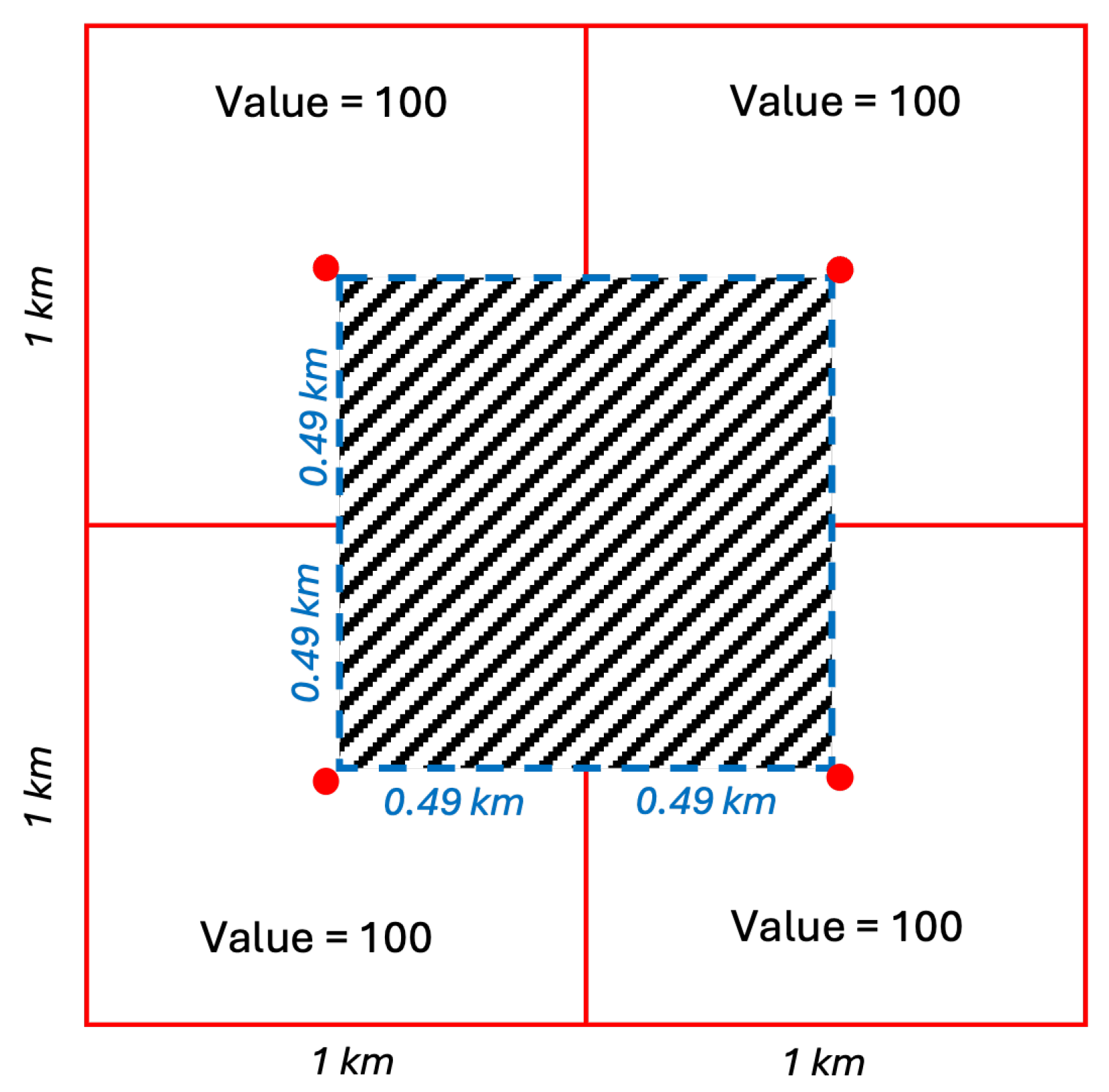
An illustrative extreme-case example of the limitations of centroid aggregation is shown in
Figure 1. While this geometric configuration is intentionally constructed to highlight a failure mode of centroid aggregation and is not representative of all polygon-grid alignments, it demonstrates that small changes in polygon placement can lead to large discontinuities in centroid-based estimates when polygons are similar in size or smaller than the underlying grid cells.
In this example, there are four adjacent 1km-by-1km grid cells in red, each of which has a value of 100; we denote the centroid for each grid cell using a red dot. If we superimpose a polygon (striped square) that measures 0.98 km along each edge and is centered at the intersection of these four grid cells, it would have a total area of 0.96 km2 but would not include any of the grid cell centroids. Thus, the centroid-based aggregation method would assign a total value of 0 to this polygon. While not shown in the figure, we also note that a small shift in the polygon vertices would adjust the estimate from a value of 0 to a value of 400; this is a large discontinuity for a very small change. Assuming that the underlying ground truth data are uniformly distributed across each of the four grid cells, the actual value of this polygon should be 96, as the representative polygon covers 24% of each grid cell. The centroid-based aggregation method not only differs significantly from the anticipated value, but in this case would represent a severe underestimate. This example visually illustrates how small geometric changes in polygon placement can produce large discontinuities in centroid-based estimates when polygon area is similar to or smaller than grid cell area. Although this example represents a worst-case scenario, it motivates the broader question explored throughout this work: under what conditions do centroid-based aggregation methods introduce substantial estimation error relative to alternative approaches?
While proportional aggregation avoids the binary inclusion–exclusion behavior associated with centroid aggregation, it may still produce substantial estimation error in cases where the underlying point distribution within a grid cell is highly heterogeneous. For example, if a polygon overlaps only a small fraction of a grid cell whose true point distribution is concentrated far from the overlap region, proportional aggregation may still substantially overestimate the true value by implicitly assuming uniform within-cell density. More generally, all grid-to-polygon aggregation approaches introduce assumptions regarding the underlying distribution of data within each raster cell. However, centroid aggregation is uniquely sensitive to small polygon shifts because the inclusion or exclusion of an entire grid cell depends solely on whether the centroid falls within the polygon boundary.
Areal interpolation is the broader family of methods commonly used when there are two distinct sets of polygons whose boundaries are not aligned, and the objective is to estimate the values of one set of polygons by re-aggregating the data from the other set of polygons [
8,
9,
10]. Within this broader class of techniques, there are several alternatives to the centroid-based aggregation method. One approach is an area-based proportional aggregation, which aggregates a fraction of each underlying grid cell’s value based on the fraction of the intersection area between each grid cell and the overlaying polygon. For example, if half of the grid cell is covered by the polygon, then half of that cell’s value is included in the aggregation. An alternative to this method is pycnophylactic interpolation which uses finite difference methods to create a smooth continuous surface while ensuring the value of each source region remains the same [
11]. It is also possible to use multidimensional resampling methods such as bilinear or cubic resampling to upsample the underlying gridded data, and then re-scale these upsampled estimates to preserve the value of each original grid cell within the resampled data. Because these methods are increasingly complex on large-scale real-world remote sensing gridded raster data, we limit our analysis in this work to bilinear interpolation with 2× and 10× upsampling factors. Another variant of areal interpolation is dasymetric interpolation which, rather than assuming the underlying data are uniformly distributed across the grid cell, which proportional aggregation assumes, instead uses a proxy dataset to weight the proportional aggregation based on the distribution of the proxy data [
12]. We exclude dasymetric interpolation as well to limit our analysis to cases in which there is no proxy data; this subset of cases is a common occurrence in real-world remote sensing data.
Contributions of this Work. In this work, we consider various sets of real-world gridded data across multiple fields of study and that exist at different spatial resolutions to observe differences between the resulting estimated value of polygons based on the centroid and proportional aggregation methods to demonstrate just how significant the impact of this choice can be in a practical setting. As real-world ground truth point data underlying many of these gridded datasets is unavailable, we conduct a series of experiments using synthetic data generated to represent the variety of statistics broadly representative of real-world geospatial distributions. In addition to centroid and proportional aggregation, we include resampling-based bilinear interpolation and quantify the error associated with each aggregation method. We conclude with a quantification of the potential consequences (relative error) of choosing sub-optimal aggregation methods, and recommendations on specific conditions under which to use each aggregation method. To the best of our knowledge, this is the first systematic quantification of the specific limitations of the centroid allocation method in comparison with other interpolation-based allocation methods.
2. Materials and Methods
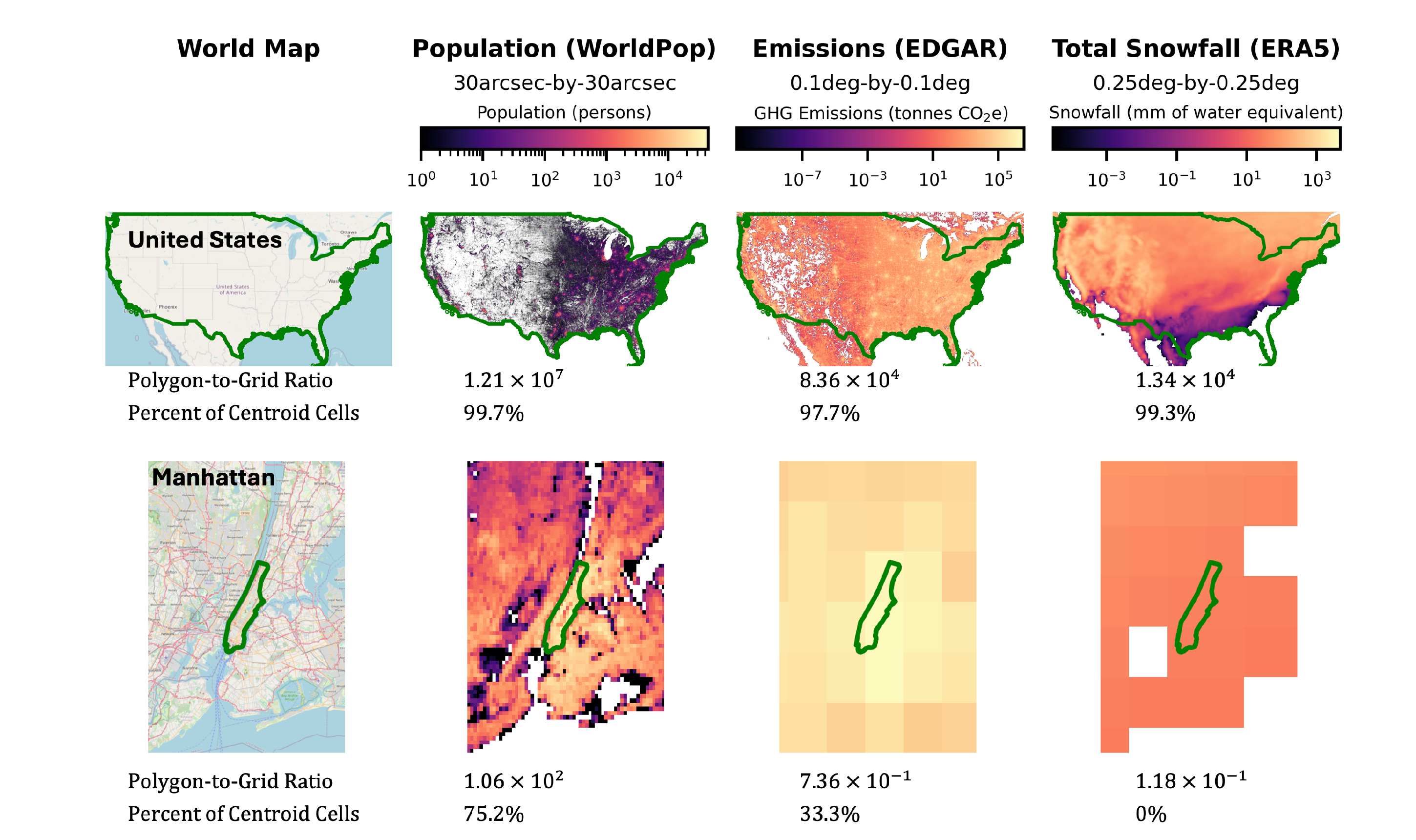
Our work is motivated by observations that estimates from grid-to-polygon aggregated data of varying spatial resolutions can be significantly impacted by the size of a corresponding overlaying polygon. As an illustrative example, in
Figure 2, we first consider two polygons of different sizes: a country-level map of the contiguous United States and a city-level map of the island of Manhattan. We visualize three different real-world underlying gridded datasets that exist at increasingly large grid cell resolutions along with each of those two polygons. The first gridded dataset, a world population dataset [
13], exists at a 30-arcsecond-by-30-arcsecond spatial resolution; the second, a global building greenhouse gas emissions dataset [
14], exists at a 0.1°-by-0.1° spatial resolution; and the third, a global total snowfall annual dataset derived from monthly snowfall data, exists at a 0.25°-by-0.25° spatial resolution [
15].
For any polygon p in the dataset we can compute metrics such as a Polygon-to-Grid Ratio (PGR) r, defined as the area of the overlaying polygon divided by the area of an individual grid cell in the gridded dataset. This gives a sense for how much larger a polygon is than a grid cell, with indicating that the polygon is larger in area than the grid cell resolution of the dataset and indicating that the polygon is no larger in area than the grid cell resolution of the dataset. We also compute the percentage of all cells touched by the polygon in which the centroid also lies within the polygon for each of the datasets of grid cells that intersect the boundary for p. We show these values for both polygons in comparison with each of the three aforementioned datasets.
Compared to the country-level boundary, all three datasets have a PGR larger than 1, indicating that the polygon size is larger than the grid cell size. The relative number of centroid-to-all-touched grid cells indicates that the vast majority of grid cells that intersect with the polygon also have a centroid falling within the polygon. Even though the spatial resolution of these three raster datasets is quite different, in comparison with a large country-sized polygon the PGR r and the centroid to all-touched proportion is similar. However, there are noticeable differences in comparison with the city-sized polygon representing the island of Manhattan. A centroid-based method would assign 100 grid cells’ data from the smallest-resolution population dataset to the island of Manhattan, whereas only a single grid cell would be assigned from the emissions dataset and no grid cells at all from the total snowfall dataset. The PGR for the latter two cases is less than 1, indicating that the polygon size is smaller than the grid cell size. For real-world data, there may be significant estimation error in aggregating gridded data within small polygons using a centroid- based method.
To quantify how the PGR (which measures the ratio of polygon area to grid cell area) impacts aggregation estimates, we use each of these three real-world datasets and aggregate raster data to polygons of varying size. In addition to using real-world country-level, county-level, and city-level boundary polygons, we also create a set of synthetic boundary polygons that we use to enhance our analysis and explore a continuum of PGRs. We emphasize that the objective of this work is not to determine an optimal raster resolution, but rather to evaluate how aggregation method performance changes as a function of the relationship between polygon size and grid cell size. Because real-world geospatial analyses involve datasets spanning a wide range of spatial resolutions and polygon scales, we intentionally vary both polygon characteristics and raster grid resolution to evaluate aggregation methods across a broad continuum of PGRs.
2.1. Gridded Datasets
The datasets we included for this evaluation were selected to span a variety of application domains and grid cell resolutions. These datasets were intentionally selected to span multiple application domains and a broad range of spatial resolutions representative of real-world geospatial raster products commonly aggregated to polygon boundaries. In particular, when measured at the equator, the selected datasets range from approximately 1km-by-1km grid cells to approximately 26km-by-28km grid cells, allowing for evaluation of aggregation behavior across substantially different PGRs. The datasets additionally represent distinct forms of spatial structure, including population density, building emissions, and climatological data.
2.1.1. Global Population
To represent our finest spatial resolution gridded dataset, we use the 2024 global population dataset from WorldPop [
13]. This global mosaic is provided in gridded form at 30arcsecond-by-30arcsecond spatial resolution (approximately 1km-by-1km at the equator). This dataset was selected to represent a commonly used fine-resolution global raster product.
2.1.2. Building Greenhouse Gas Emissions
At coarser spatial resolution, we use the 2024 building emissions dataset from the EDGAR Emissions Database for Global Atmospheric Research [
14]. The EDGAR global emissions gridded dataset represent tonnes of greenhouse gas (GHG) emissions in units of CO
2e at a spatial resolution of 0.1°-by-0.1°(approximately 11km-by-11km at the equator). This dataset was selected to represent a moderate-resolution global environmental dataset commonly used in policy and sustainability applications.
2.1.3. Total Snowfall
At our coarsest spatial resolution, we use a 2024 total annual snowfall dataset derived from ERA5 monthly snowfall data [
15]. The total snowfall gridded dataset represents total annual snowfall in units of mm of water equivalent at a spatial resolution of 0.25°-by-0.25°(approximately 28km-by-28km at the equator). This dataset was selected to represent a comparatively coarse-resolution climatological raster product.
2.2. Geospatial Polygon Boundaries
2.2.1. Country-Level Boundaries
The largest geospatial boundaries that are typically considered for grid-to-polygon data aggregation tasks are country-level boundaries. GADM is an open-source project that “wants to map the administrative areas of all countries, at all levels of sub-division” [
16]. The Level 0 subdivision contained within the GADM Database of Global Administrative Areas is our source for country-level boundaries. The latest version of this database contains boundaries for 267 countries at the Level 0 subdivision. The average country boundary size is approximately 560,000 km
2, making these the largest boundaries under consideration.
2.2.2. County-Level Boundaries
We also use GADM [
16] for county-level or district-level boundaries, reflected by the GADM Level 2 subdivision. The latest version of this database contains boundaries for 47,217 administrative regions at the Level 2 subdivision. The average county boundary size is approximately 2800 km
2.
2.2.3. City-Level Boundaries
We use the Functional Urban Area boundaries from the Global Human Settlements Layer (GHS-FUA), which “delineate the spatial entities representing the commuting area of the Urban Centres of 2015,” [
17,
18] for our city-level boundaries. These boundaries collectively represent a population of approximately 3.9 billion people (54% of the 2015 global population). The latest version of this database contains boundaries for 9031 Functional Urban Areas from 188 distinct countries across the world. The average FUA boundary size is approximately 281 km
2.
2.2.4. Synthetic Boundaries
To ensure a broader representation of potential boundary sizes than those available to us in the above real-world sources, we further generate square polygon boundaries to use as a synthetic boundary dataset. We first fix an area size to ensure all polygons are identical in size (in degrees latitude/longitude), and then generate 1000 polygons for each fixed size. We replicate this process across a range of polygon sizes. We draw the location of the polygon centroid from a random uniform distribution, and we impose two restrictions on any such generated polygon: (1) the centroid of the polygon must fall within the land surface of the earth, and (2) the edges of the polygon must entirely fall within the two-dimensional bounding box outlining the world map. We replicate this process across a range of fixed polygon sizes, ensuring that there are exactly 1000 synthetic polygons generated for each choice of fixed polygon size. The smallest area size that we choose corresponds to a square on the order of magnitude of a New York City block. The largest area size that we choose corresponds to a square approximately the size of the country of Switzerland.
2.3. Comparison Across Real-World Data and Boundaries
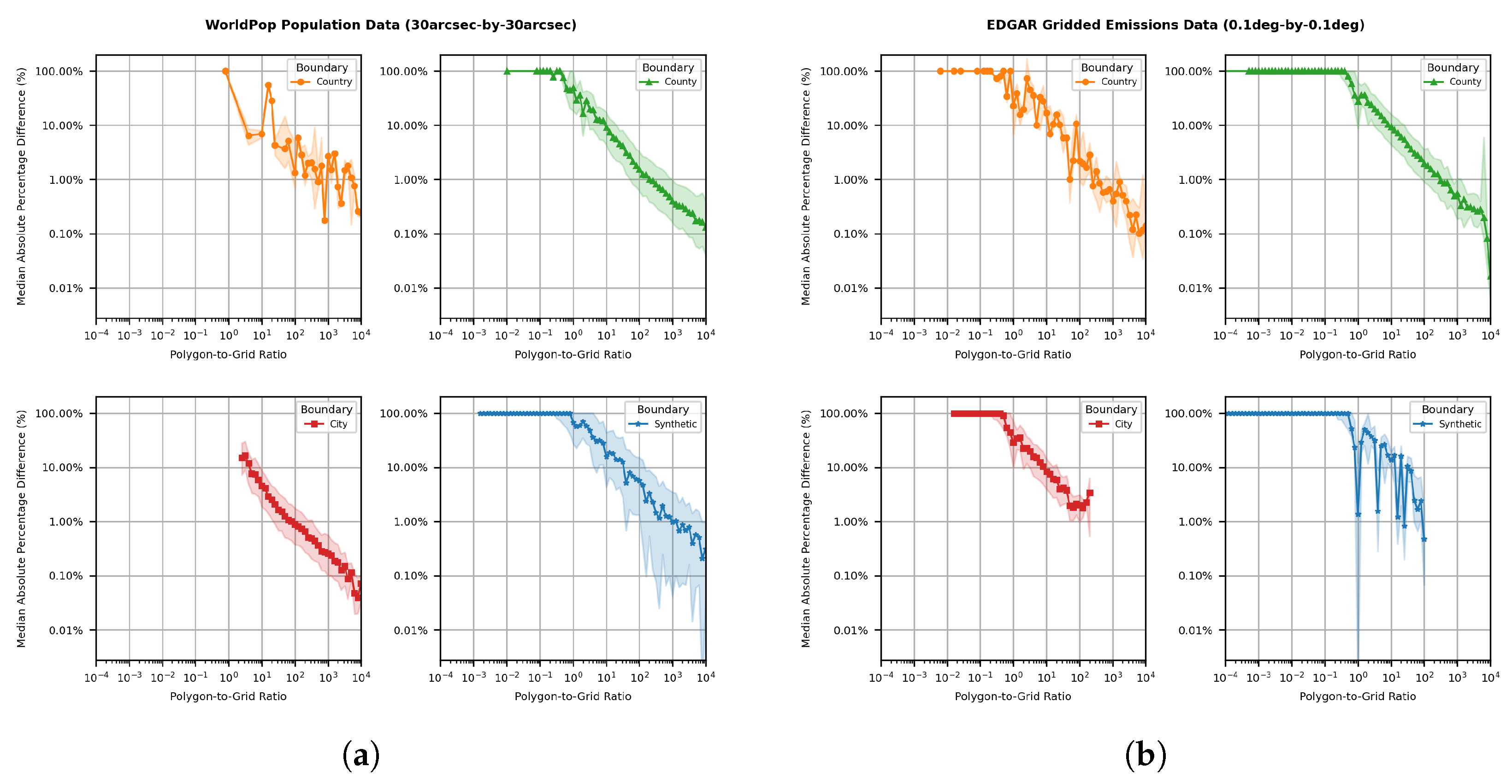
We consider the percentage difference between the centroid and proportional aggregation methods as a mechanism to compare their relative performance in aggregating real-world gridded data. We compute the PGR and bin all polygons corresponding to that ratio by 1/10-decade steps. We display the median absolute percentage difference as a function of PGR, independently considering each of our four sets of geospatial polygon boundaries as described previously in
Section 2.2. The shaded region in each of these plots corresponds to the interquartile range, i.e., the 25th to 75th percentile of data. We also remove any cases in which the centroid and proportional aggregation methods both estimate a value of 0. In
Figure 3, we show the percentage difference comparisons for the WorldPop and EDGAR datasets, and the comparison for the Total Snowfall dataset is included in
Appendix A.
While the specific underlying gridded data are different and each dataset exists at a different spatial resolution, we observe a key trend common to all real-world datasets. At large PGRs (i.e., cases in which the polygon area is vastly larger than the grid cell area) the median absolute percentage difference (MAPD) converges to a 0% difference, but the size differences between the area of the polygon and the area of the grid cells need to be several orders of magnitude for this to be true, which is commonly not the case in real-world settings. As PGRs decrease, the MAPD increases with a significant difference between the two aggregation approaches when the polygon area is similar in size or smaller than the grid cell area.
Table 1 provides additional detail associated with these observed differences shown in
Figure 3. The finer-resolution WorldPop dataset exhibited relatively small differences across all evaluated boundaries, with median absolute percentage difference below 1%. In contrast, the coarser-resolution EDGAR emissions and snowfall datasets exhibited substantially larger differences, particularly for the smaller polygon boundaries such as the county- and city-level boundaries. For the EDGAR emissions dataset, the median absolute percentage difference between centroid and proportional aggregation increased from 1.0% at the country scale to 14.8% at the county scale and 100.0% at the city scale. More than 85% of city-scale polygons differed by over 10% while more than 60% of polygons differed by over 50%. Similar trends were observed for the snowfall dataset. Together, these results demonstrate that the aggregation behaviors observed in the synthetic experiments emerge systematically across multiple real-world datasets and become increasingly consequential as raster resolution becomes coarse relative to the polygons used for downstream analysis.
While this demonstrates that there is the potential for significant differences between aggregation approaches, it does not inform which approaches are preferable and under what conditions. For that, we rely on synthetic data experiments.
2.4. Synthetic Data Experimentation
Although we are able to use real-world gridded data to quantify the percentage differences between aggregation methods to provide examples of the potential impacts, a lack of ground truth point data restricts our ability to quantify the percentage error of each approach. We thus define a set of experiments using synthetic point process data that are representative of real-world data. These synthetic points are used as ground truth values, with which we form a basis for comparison against various grid-to-polygon aggregation methods.
2.4.1. Problem Formulation
We first define the key components of this problem and metrics we will use to compare aggregation method performance. We define
r as the PGR and
c as the grid cell area size. For each pair
, we generate a set of
n polygons, i.e.,
. Each polygon sample
has a corresponding ground truth value
which is the true value of synthetic samples that lie within the polygon. We denote each aggregation method as
for the
jth aggregation method. The estimated aggregate value from method
j on sample
i is defined as
for any combination of
r and
c and the corresponding absolute error is
:
To evaluate the performance of method
for a given pair
, we primarily use the Weighted Absolute Percentage Error (WAPE) metric. The WAPE metric more heavily penalizes prediction errors in samples with larger ground truth values, which is desirable to understand the impact of aggregation error. We secondarily consider the Median Absolute Percentage Error and Mean Absolute Error metrics, both of which are described in
Appendix A.
To complement the performance evaluation using WAPE, we also evaluate the number of times each aggregation method
outperforms the other aggregation methods. We define the lowest-error set
as the set of polygons
for which aggregation method
is better than all other methods:
We use
to define a proportion of lowest-error cases,
for a given aggregation method
and a pair of
r and
c as (where
represents cardinality of the set)
2.4.2. Generating Synthetic Data and Boundaries
There are several approaches to generating spatial point processes [
19]. We use three statistical models to synthesize our ground truth point data, with parameters chosen for those models to represent a wide range of potential variability. On one end of the spectrum of spatial correlation, we include the case of complete spatial randomness and represent it through a homogeneous Poisson process. As we consider greater degrees of spatial correlation, we also explore inhomogeneous Poisson process models, which can be used to synthesize points that are spatially clustered and represent several real-world data settings [
20]. In particular, we consider two specific types of inhomogeneous Poisson process models, the Neyman–Scott process model and the Log-Gaussian Cox process model, to cover several potential real-world settings.
The Neyman–Scott process [
21] has been used to produce clustered patterns of data represented by a “parent–child” structure; although the root of this model is in cosmology, data distributed according to this point process also exist in disease mapping and many ecological relationships such as seed/tree dispersion [
19,
22,
23,
24,
25,
26]. To generate synthetic data using this process, the Neyman–Scott model first places parent points across space, typically via a homogeneous Poisson process. Each of these parent points then generates a number of child points with locations distributed in the vicinity of the parent point.
The Log-Gaussian Cox process [
27] has also been used to model spatial point process data in domains such as population, disease risk to include mapping cancer mortality, and health surveillance in cases such as bovine tuberculosis [
28,
29]. This model uses a Gaussian process to generate spatially correlated random values across a continuous field, and then uses an inhomogeneous Poisson process to generate placement of points, with more points falling in the higher-field-intensity regions and fewer points falling in the lower-field-intensity regions.
We generate four distinct sets of synthetic data based on these three spatial point processes to cover a variety of statistical settings. Summary spatial statistics for these data are included in
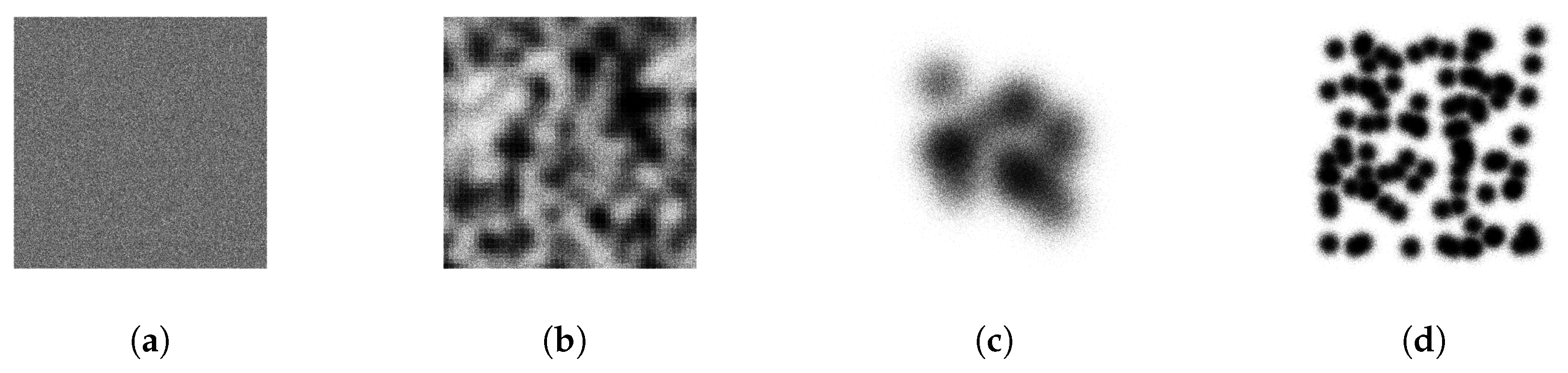
Appendix A. We generate one set of synthetic data using the homogeneous Poisson process model. We generate two sets of synthetic data using the Neyman–Scott process model, one of which represents a case of many small dense clusters and the other representing a case of fewer large dispersed clusters. We finally use the Log-Gaussian Cox process to reflect similarities present in population and disease risk cases. The four sets of synthetic point process data that we generate are shown in
Figure 4.
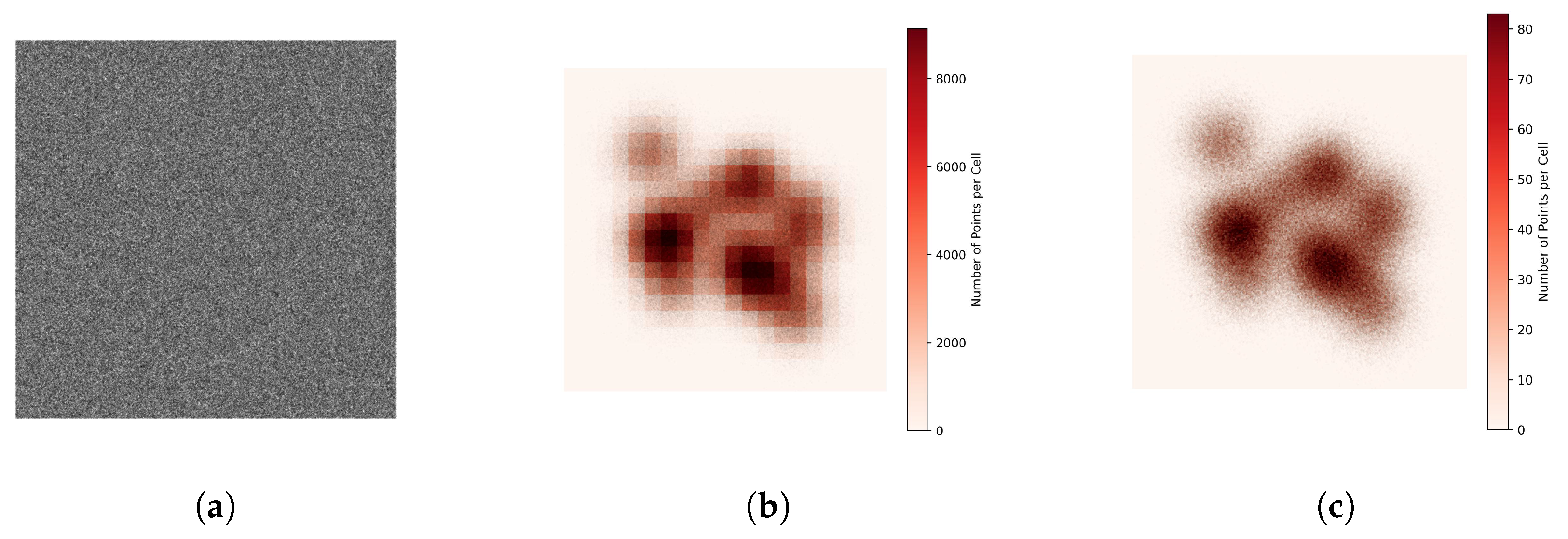
To replicate real-world geospatial gridded raster data, we then rasterize these large point datasets by rasterizing these points; the value assigned to each grid cell is simply the count of points within each grid cell. For our experimentation, we use two different grid cell sizes
c: an 0.1°-by-0.1°grid cell size, and an 0.00833°-by-0.00833°grid cell size. These correspond to approximately 11km-by-11km and 1km-by-1km grid cells, respectively, if the grid cells were located at the equator. The use of multiple grid cell resolutions is intended to evaluate aggregation method behavior across different PGRs rather than to compare the intrinsic quality of the raster resolutions themselves. An example of this rasterization process using the Large Dispersed Neyman–Scott synthetic point process data is shown in
Figure 5.
We also generate a new set of polygons to use for evaluating the efficacy of different aggregation for these data. We generate sets of 1000 synthetic polygons for each chosen polygon step size, resulting in 61 distinct step sizes and 61,000 total synthetic polygons for our synthetic data experimentation. We then estimate the value associated with each polygon using each of our aggregation methods that we compare here (introduced below) and compare to the ground truth for evaluation.
2.4.3. Grid-to-Polygon Aggregation Methods
To evaluate the variety of grid-to-polygon aggregation approaches, we compare four different methods
. We first consider centroid aggregation, the most commonly used today, as our baseline method. We also compare proportional aggregation, which only factors in the fraction of the value from each cell proportional to its degree of overlap with the aggregating polygon. Lastly, we include resampling-based bilinear interpolation using two different upsampling factors. We investigate this for a 2× upsampling case (which we reference as interpolation-2×- bilinear) and a 10× upsampling case (which we reference as interpolation-10×-bilinear). We also explored additional upsampling factors beyond these two choices for bilinear interpolation. We limited our experimentation to these two choices to serve as a balance between expected performance and computational tractability. Additional detail on the bilinear interpolation is available in
Appendix A.
3. Results
We evaluate each of the four aggregation methods described above, centroid, proportional, and 2× and 10× bilinear interpolation across a range of PGRs to compare the performance across methods when there is known (albeit synthetic) ground truth.
3.1. Synthetic Aggregation Behavior Across PGRs
We evaluate aggregation methods
within each subset
for each of the four different sets of synthetic ground truth points. For a given subset
, we first remove all samples containing a ground truth value of 0 to ensure that all polygons being considered contain at least one point, i.e.,
. We use the WAPE metric
as our primary error metric to reflect the balance between error and the ground truth values of samples within each PGR subset
. Results computed using additional metrics are provided in
Appendix A.
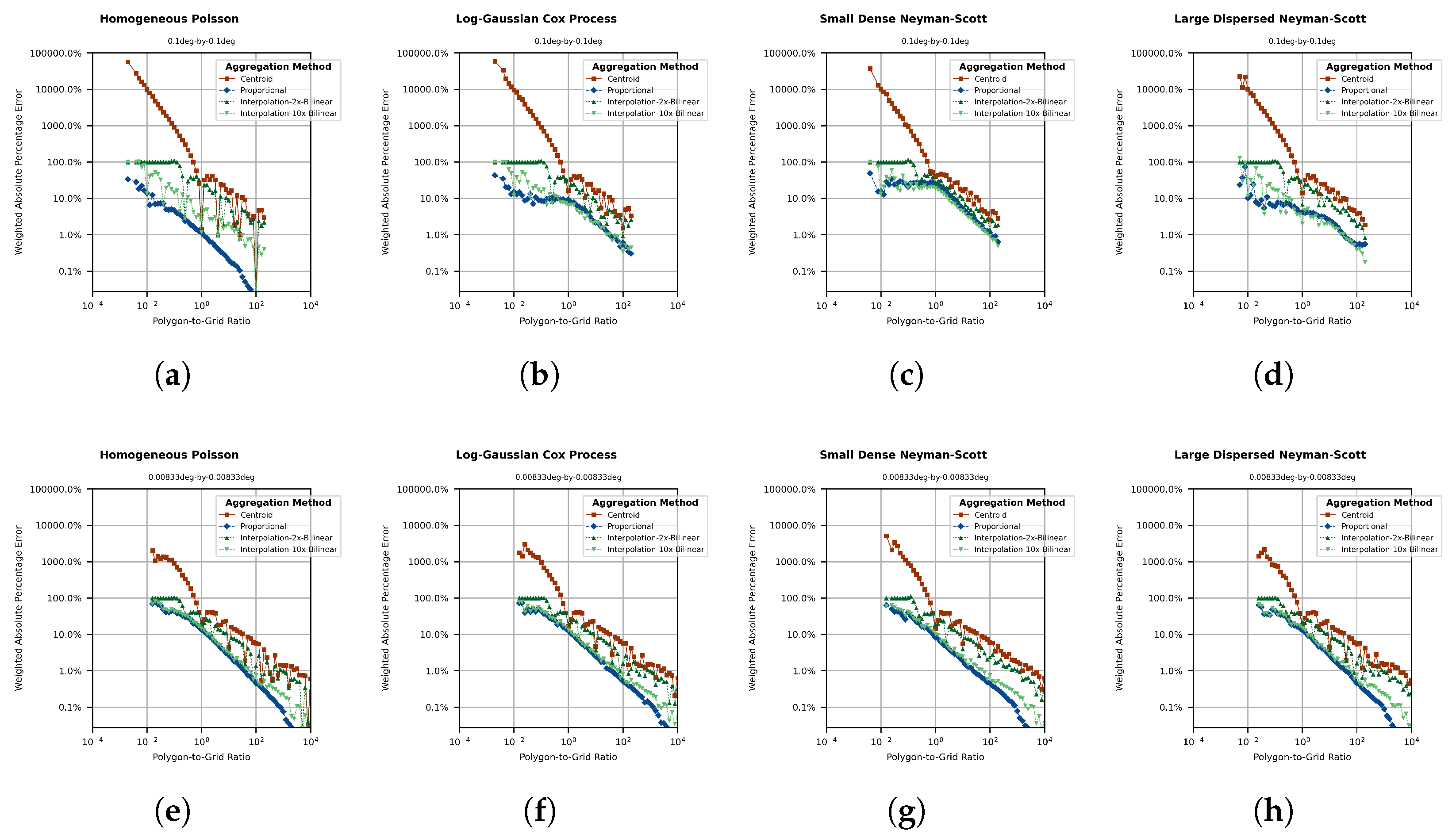
We compute
for each method
and each pair
, replicating this process across each of the four distinct sets of ground truth data points. The resulting WAPE values are shown in
Figure 6.
These results reinforce our earlier observations from real-world data that there is a significant difference between the centroid aggregation method and other aggregation methods. We observe that centroid aggregation tends to underperform in almost all settings as compared to other methods. We also observe that regardless of the underlying data distribution, all methods converge toward relatively smaller error as the polygon becomes several orders of magnitude larger than the grid cell size; however, the rate of convergence and acceptable error levels remain dependent on the underlying spatial distribution and application context. We further observe that the WAPE from the centroid method grows at a significantly higher rate than the other three aggregation methods when the PGR shrinks below 1.
Figure 6 visually demonstrates that this divergence becomes increasingly pronounced as the polygon area approaches or falls below the grid cell area. This is particularly notable in the upper row of
Figure 6, the scenarios with the larger grid cell sizes. While generally the centroid aggregation method does poorly, there are anywhere between 4.6% and 16% of samples in which the centroid aggregation method has lower error than the other methods; we explore this in the context of the
metric in
Appendix A.
From a computational perspective, the centroid method is algorithmically simpler than the other three methods. All four methods require a point-in-polygon test for each grid cell in the dataset to determine if a grid cell intersects with a given polygon. For the centroid method, the point-in-polygon test is the only computation required; all the other methods then require additional computational processes using those grid cells assigned to the polygon based on passing the point-in-polygon test. However, in practice, proportional aggregation using a sufficiently efficient implementation (e.g., from the exactextract Python package) was found to be faster than any of the other three methods when aggregating our synthetic raster data to our synthetic polygons. We believe this practical speed advantage is largely attributable to the highly optimized underlying implementation used by exactextract relative to the native Python implementations used for several of the alternative aggregation approaches considered. It is also likely that if a centroid aggregation approach were similarly optimized, we would see decreased compute time as compared to the native Python implementations of that approach. The compute time results across our eight different synthetic datasets are summarized in
Table 2, and we provide additional details in
Appendix A.
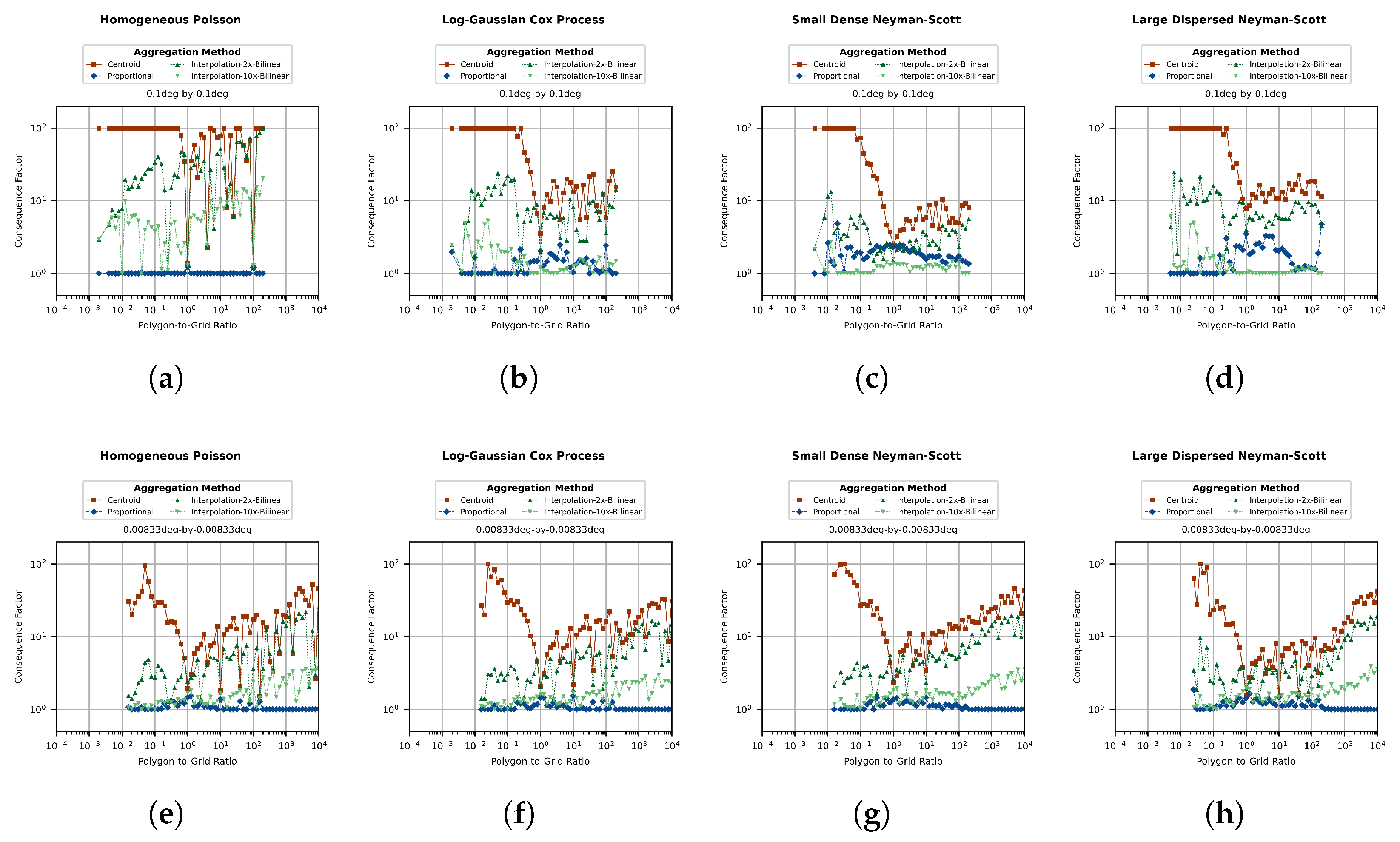
3.2. Consequences of Sub-Optimal Aggregation Method Selection
For each PGR, there is generally one method that outperforms the other aggregation methods on average. However, there is some degree of per-sample variation for which method may be best. We can use this to capture the difference in error between the best possible choice and each other method when that best possible choice is not chosen, to demonstrate the potential gap in performance for sub-optimal aggregation method selection.
To quantify the consequence of choosing a sub-optimal aggregation method, we note that each polygon
has an associated ground truth value
, and each aggregation method
j is used to compute an estimated value
. We define the best method
for sample
as
The best estimated value for polygon
is the estimated value produced by that aggregation method:
For any aggregation method, we can then compute a consequence factor (CF) in comparison with that best value
for each sample
as follows:
To ensure that the CF metric is always defined, if both and exactly equal the ground truth value , we set the CF as 1. If exactly equals but the estimate is a different value, we set the CF as 100. We are also assured that for each polygon , one of the CF values will always be exactly 1, as one of the aggregation methods will always be best.
We can use this CF to directly measure the impact of choosing the sub-optimal aggregation method as a function of the PGR. A CF of 1 suggests that both methods would result in equal error estimates as compared to ground truth. A CF larger than one suggests a larger relative disparity between the optimal and sub-optimal method. For example if the consequence factor is 2, it would imply that the error for the selected method is twice as large as the optimal approach. For each combination of synthetic data distribution and grid cell size
c, we plot the median CF for all four aggregation methods in
Figure 7.
We generally observe across all of our synthetic data that the CF is less than 10 for the cases in which centroid aggregation is best, but another aggregation method is chosen. More importantly, for PGR values less than one, i.e., , we observe a much more significant CF for the cases in which centroid aggregation is chosen but is not best. In particular, the error could be more than 100× as large (indicated by a CF ) in these cases. This provides experimental evidence that for small PGRs—i.e., cases in which the polygon is smaller than the grid cell—the consequence of choosing to use centroid aggregation and centroid not being optimal is far more significant than the consequence of choosing to use any other aggregation method and choosing incorrectly.
4. Discussion
The results of this work demonstrate several key findings that inform recommendations for best practices in grid-to-polygon aggregation and under what conditions different aggregation alternatives should be chosen. Across the synthetic experiments, proportional aggregation or 10× bilinear interpolation generally produced the lowest error. However, centroid aggregation may still be acceptable when the polygon area is substantially larger than the grid cell area. In particular, when the PGR is several orders of magnitude greater than 1, all methods approach relatively low error, and centroid aggregation may be appropriate when computational simplicity, software compatibility, or reproducibility with existing workflows is prioritized. For PGR values near or below 1, where polygon area is similar to or smaller than grid cell area, centroid aggregation becomes much more sensitive to polygon placement and can produce substantially larger errors than the alternatives. In these settings, proportional aggregation is generally the preferred default because it performs well across most experiments and can be implemented efficiently. If computation is not a significant constraint, then high levels of upsampling and bilinear interpolation may also be appropriate in some cases, particularly where interpolation better reflects assumptions about the underlying spatial surface. The acceptable level of aggregation error ultimately depends on the downstream application, recognizing that some use cases may tolerate several percent estimation error while others may require substantially greater precision.
More generally, the PGR provides a practical mechanism for guiding aggregation method selection. For cases in which the PGR is substantially greater than 1, centroid aggregation may provide sufficiently low error for many applications. As the PGR approaches 1, boundary effects become increasingly important and proportional aggregation is generally preferable. For PGR values less than or equal to 1, where polygon area is similar to or smaller than grid cell area, centroid aggregation may produce severe estimation error and proportional aggregation or interpolation-based methods should generally be used instead. While no universal thresholds apply across all applications, the results suggest that the aggregation method choice becomes increasingly consequential as the PGR decreases.
Limitations and Future Directions
One limitation to our research is overcoming the lack of ground truth data with which to completely understand the difference across different grid-to-polygon aggregation methods in real-world settings. While we explored a range of statistical properties, real-world data would have been preferable.
Another limitation is that while this work explored the PGR as a key characteristic that may impact performance, the synthetic point process models considered here do not fully capture all forms of real-world spatial heterogeneity. In particular, we did not explicitly model boundary-dependent or non-stationary spatial processes that may arise in certain environmental, climatological, or socio-economic datasets. While we explored a range of clustering structures and spatial autocorrelation regimes using multiple point process models, additional research is warranted to evaluate aggregation method performance under more complex spatial processes and polygon geometries representative of specific real-world applications.
Although the synthetic experiments intentionally used simplified square polygons to isolate the effects of polygon-grid geometry and relative scale, real-world polygons often exhibit substantially more complex geometries, including concave and multi-scale boundaries. Our real-world analyses suggest that the observed aggregation behaviors generalize across realistic geographic boundaries, but future work could more explicitly investigate the role of polygon shape complexity on aggregation-method performance.
5. Conclusions
In this work, we investigated the relative efficacy of what is the default choice in many practical applications of grid-to-polygon aggregation: centroid-based aggregation. Our findings suggest that centroid aggregation is rarely an optimal choice and, whenever feasible, efficient alternative approaches such as proportional aggregation or combinations of upsampling and bilinear interpolation should be used to minimize the estimation error for grid-to-polygon aggregation.
The findings of this work demonstrate that centroid aggregation frequently results in substantially higher error rates than alternative aggregation approaches across many practical settings. Across multiple real-world datasets, we observe that aggregation-method differences emerge systematically across common real-world geographic boundaries. In particular, coarse-resolution raster datasets exhibited increasingly severe differences between centroid and proportional aggregation at county- and city-scale boundaries, while finer-resolution datasets exhibited comparatively small differences across the same geographic definitions. These findings demonstrate that aggregation-method selection can materially influence downstream estimates in common real-world geospatial analysis workflows.
We conducted several experiments to quantify the error of aggregating gridded raster data to polygons when trying to estimate the value of the gridded data within the boundary of those geospatial polygons as well as the impact of choosing a sub-optimal aggregation method. These experiments are designed to isolate how aggregation error changes as a function of polygon-grid geometry and relative scale rather than to recommend a universally optimal raster resolution. The conventional approach of using centroid aggregation when aggregating real-world data to geospatial polygons has deficiencies with potentially severe consequences. Compared to proportional aggregation and upsampling plus bilinear interpolation, we quantified the performance differences across these approaches using synthetically generated point process data and investigated the impact of the PGR and the underlying grid cell size on expected performance. We generated four unique synthetic ground truth point datasets using including homogeneous Poisson process, Log-Gaussian Cox process, and Neyman–Scott processes. In addition to the centroid and proportional aggregation approaches, we compared upsampling gridded data via bilinear interpolation to introduce two additional aggregation methods as part of our synthetic data experimentation using both and upsampling factors.
While this is true in almost every setting, this is especially significant for PGRs smaller than 1, when the polygon area is no larger than the grid cell area. Although the centroid method rarely outperforms the other aggregation methods, in the limit as the PGR increases to infinity, all aggregation methods converge to the ground truth value. However, for many commonly encountered cases in which the polygon area is not orders of magnitude larger than the grid cell area, the centroid method is sub-optimal and may have 100× the error of the other aggregation methods in extreme cases. Across both the synthetic and real-world experiments, the severity of these differences increased substantially as raster resolution became coarse relative to the polygon boundaries used for downstream analysis. We, therefore, recommend selecting aggregation methods based on the PGR, with particular caution in low-PGR settings where the polygon area is similar to or smaller than the grid cell area.
Author Contributions
Conceptualization, Paul J. Markakis, Jordan M. Malof, Leslie Collins and Kyle Bradbury; methodology, Paul J. Markakis, Jordan M. Malof, Leslie Collins and Kyle Bradbury; software, Paul J. Markakis and Kyle Bradbury; validation, Paul J. Markakis; formal analysis, Paul J. Markakis; investigation, Paul J. Markakis; resources, Leslie Collins and Kyle Bradbury; data curation, Paul J. Markakis; writing—original draft preparation, Paul J. Markakis; writing—review and editing, Jordan M. Malof, Leslie Collins and Kyle Bradbury; visualization, Paul J. Markakis; supervision, Leslie Collins and Kyle Bradbury; project administration, Kyle Bradbury; funding acquisition, Kyle Bradbury. All authors have read and agreed to the published version of the manuscript.
Funding
The authors would like to thank the Climate TRACE coalition for its organizational support, and Climate TRACE’s funders for their financial support. For a full list of funders, please visit the Climate TRACE website:
https://climatetrace.org/team (accessed on 1 May 2026).
Data Availability Statement
The original contributions presented in this study are included in the article, and the method used to generate all data are described within the manuscript. Further inquiries can be directed to the corresponding author(s).
Acknowledgments
The authors would like to thank the Climate TRACE coalition for its organizational support, and Climate TRACE’s funders for their financial support. For a full list of funders, please visit the Climate TRACE website:
https://climatetrace.org/team (accessed on 1 May 2026).
Conflicts of Interest
The authors declare no conflicts of interest. The funders had no role in the design of the study; in the collection, analyses, or interpretation of data; in the writing of the manuscript; or in the decision to publish the results.
Appendix A
Appendix A.1. Additional Real-World Data
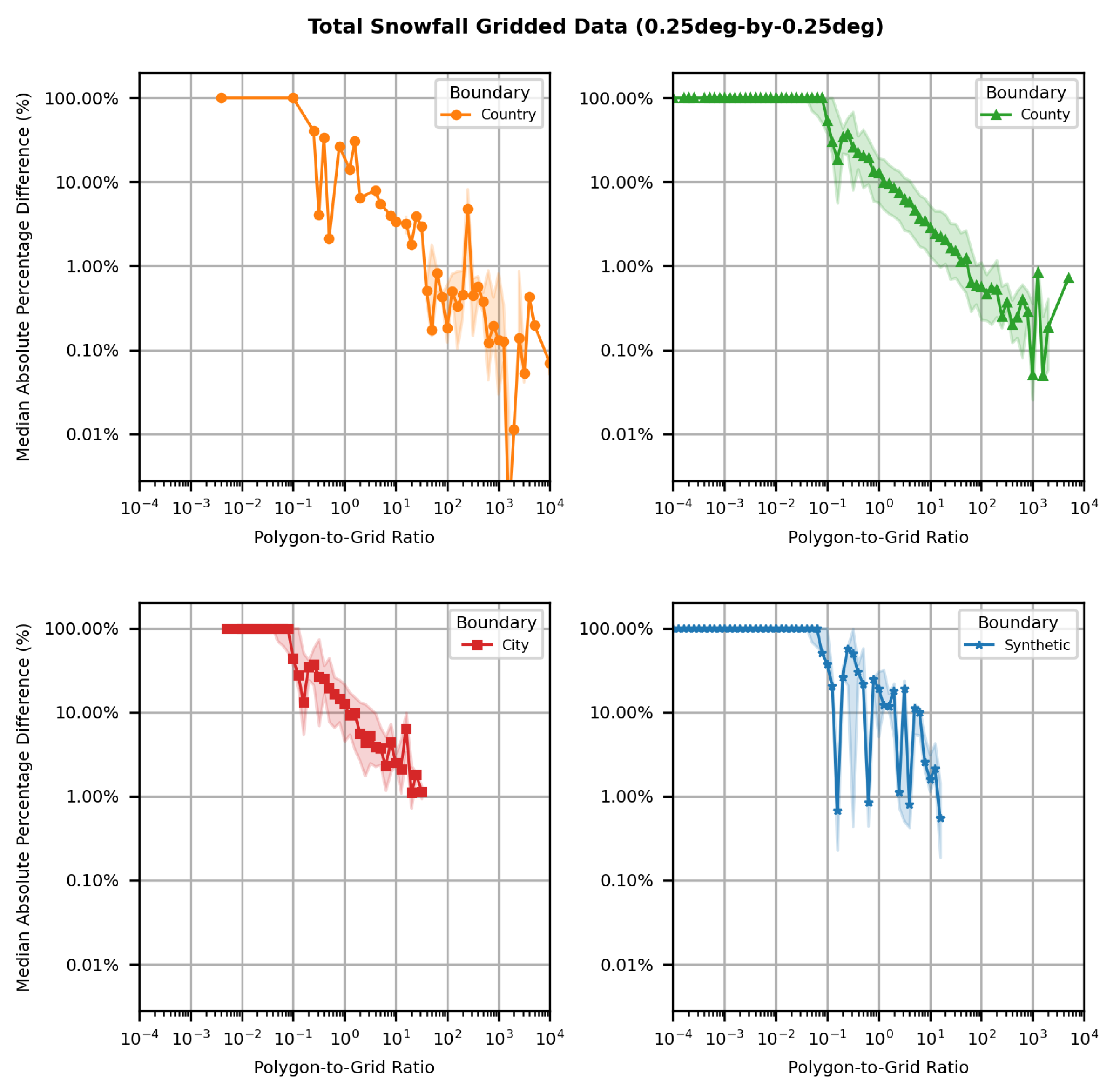
We additionally include the median absolute percentage difference results below for the total snowfall dataset. We observe similar trends to the WorldPop population data and EDGAR emissions data.
Figure A1.
Median absolute percentage differences as a function of PGR for real-world gridded total snowfall dataset with 0.25°-by-0.25°spatial resolution. These data show that as the PGR increases, the percentage difference between centroid and proportional aggregation approach 0%, suggesting that both methods estimate the same value; however, for smaller PGRs and especially PGR ≤ 1, there could be differences up to 100% between the estimates from the two methods.
Figure A1.
Median absolute percentage differences as a function of PGR for real-world gridded total snowfall dataset with 0.25°-by-0.25°spatial resolution. These data show that as the PGR increases, the percentage difference between centroid and proportional aggregation approach 0%, suggesting that both methods estimate the same value; however, for smaller PGRs and especially PGR ≤ 1, there could be differences up to 100% between the estimates from the two methods.
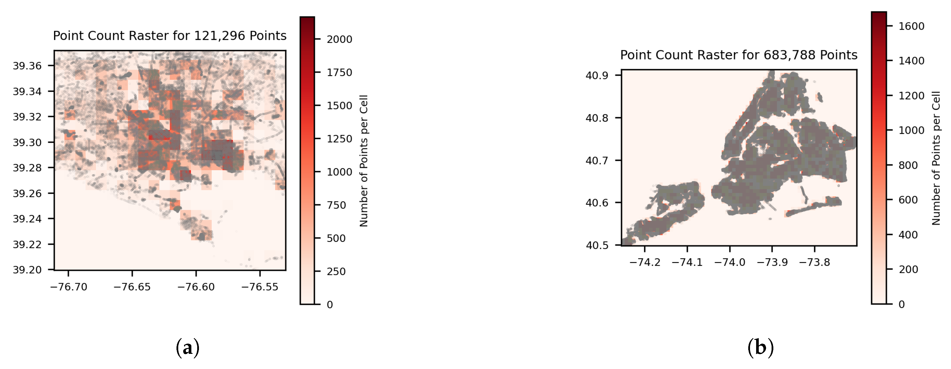
Additional real-world datasets were also used to inform choices for data distributions and parameters associated with representative real-world data. Below are plots from a dataset of tree inventories from two major cities in the United States [
30] showing the distribution of ground truth points for individual trees in each of these cities. These are visually similar to the Neyman–Scott synthetic data distributions, reinforcing that choice of distribution and informing the parameters chosen for those point process models in our synthetic data generation process.
Figure A2.
Distribution of individual trees in major USA cities, with Baltimore shown in (a) and New York in (b). These are overlaid with a 0.00833°-by-0.00833°grid. We observe the similarities between these data and the Small Dense Neyman–Scott synthetic data samples.
Figure A2.
Distribution of individual trees in major USA cities, with Baltimore shown in (a) and New York in (b). These are overlaid with a 0.00833°-by-0.00833°grid. We observe the similarities between these data and the Small Dense Neyman–Scott synthetic data samples.
Appendix A.2. Spatial Statistics for Real-World and Synthetic Data
We include key spatial statistics for both real-world and synthetic data. We first measure the density of points, including the number of points per unit area as well as computing the mean and standard deviation number of points in each nonzero grid cell. We also consider the Moran’s I measure of autocorrelation, which has a value of 0 if data are uncorrelated and approaches 1 for stronger measures of autocorrelation within a dataset [
31]. These are shown in
Table A1.
Table A1.
Spatial statistics summary.
Table A1.
Spatial statistics summary.
| Dataset | Resolution | Number of Points per Unit Area | Nonzero Points per Grid Cell | Global Moran’s I |
|---|
| EDGAR | 0.1°-by-0.1° | 54,776 | 4026 ± 25579 | 0.596 |
| WorldPop 1 | 0.00833°-by-0.00833° | 156,767 | 158 ± 812 | - |
| Baltimore Trees | 0.00833°-by-0.00833° | 3,611,695 | 355 ± 345 | 0.713 |
| NYC Trees | 0.00833°-by-0.00833° | 2,898,361 | 557 ± 352 | 0.798 |
| Homogeneous Poisson | 0.1°-by-0.1° | 300,239 | 3001 ± 52.7 | 0.046 |
| Homogeneous Poisson | 0.00833°-by-0.00833° | 295,533 | 20.6 ± 5.0 | 0.156 |
| Small Dense Neyman–Scott | 0.1°-by-0.1° | 329,829 | 3481 ± 3759 | 0.397 |
| Small Dense Neyman–Scott | 0.00833°-by-0.00833° | 324,660 | 32.8 ± 33.9 | 0.968 |
| Large Dispersed Neyman–Scott | 0.1°-by-0.1° | 124,929 | 1557 ± 2057 | 0.910 |
| Large Dispersed Neyman–Scott | 0.00833°-by-0.00833° | 122,970 | 16.8 ± 15.6 | 0.956 |
| Log-Gaussian Cox Process | 0.1°-by-0.1° | 377,795 | 3778 ± 2448 | 0.646 |
| Log-Gaussian Cox Process | 0.00833°-by-0.00833° | 371,873 | 26 ± 19.4 | 0.906 |
Appendix A.3. Aggregation Method Implementation Details
All of our grid-to-polygon aggregation methods are implemented in Python 3.9 using existing packages.
Centroid Aggregation. We use the rasterstats module, which is a native Python module based on numpy for computing zonal statistics [
32].
Proportional Aggregation. We use the exactextract module, which offers a Python module that leverages a C++ backbone to conduct proportional aggregation efficiently [
33,
34]. While conceptually the proportional aggregation method is more complex than centroid aggregation, the computational enhancements from the C++ backbone for proportional aggregation via exactextract lead to it being faster in practice than native Python methods for centroid aggregation, as evidenced in this work.
Bilinear Interpolation. To resample the source gridded data, we use the rasterio module, which is a native Python module for processing raster data [
35]. We then use the rasterstats module with centroid aggregation to aggregate the resampled data within polygons.
Appendix A.4. Resampling-Based Bilinear Interpolation
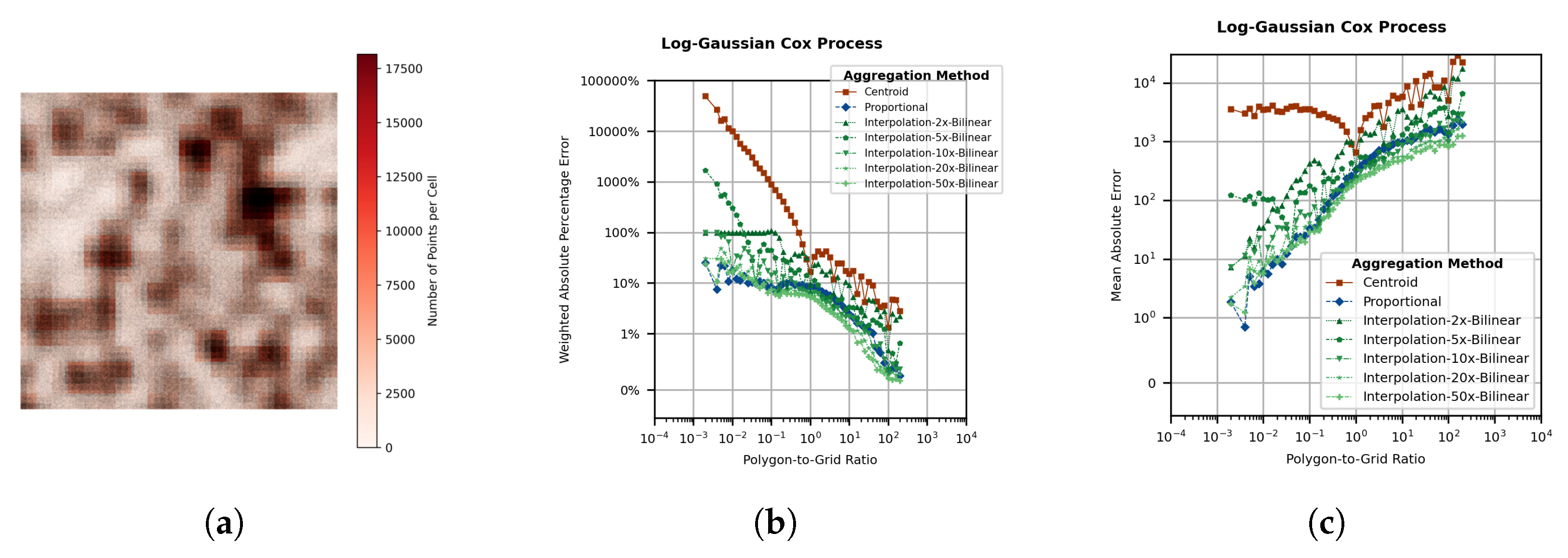
We conduct additional analysis to justify our choices of parameters for bilinear interpolation. We consider upsampling factors of 2×, 5×, 10×, 20×, and 50× to represent a range of possible levels of resolution. Recognizing that there are similarities across data distributions and that methods generally tend to be consistent with raster resolution of 0.00833°-by-0.00833°, we only consider a single data distribution (a Log-Gaussian Cox process) and a single raster resolution of 0.1°-by-0.1°. In
Figure A3, we show the synthetic raster data generated for this sub-experiment as well as the WAPE and MAE across all aggregation methods. We observe that the Interpolation-5×-Bilinear model is actually worse than the Interpolation-2×-Bilinear model, and that there is not a significant decrease in error for values beyond a 10× upsampling factor (reflected by the Interpolation-20×-Bilinear and Interpolation-50×-Bilinear models).
Table A2 summarizes the raster size for each of the model variants. We observe that there is a 4x increase in raster size going from the Interpolation-10×-Bilinear model to the Interpolation-20×-Bilinear model and a 25× increase in raster size for the Interpolation-50×-Bilinear model. We thus choose to retain the Interpolation-2×-Bilinear and Interpolation-10×-Bilinear models as our comparison models to reflect the best balance between low error and raster size.
Figure A3.
Exploration of various bilinear interpolation upsampling factors using 0.1°-by-0.1°gridded synthetic data. In (a) we show the raster data with the underlying ground truth point data, while in (b,c) we show the WAPE and MAE for various aggregation methods including centroid and proportional methods as well as several different choices of upsampling factor. Although we do see a reduction in error as upsampling factor increases, the 10×, 20×, and 50× upsampling factors result in fairly similar error.
Figure A3.
Exploration of various bilinear interpolation upsampling factors using 0.1°-by-0.1°gridded synthetic data. In (a) we show the raster data with the underlying ground truth point data, while in (b,c) we show the WAPE and MAE for various aggregation methods including centroid and proportional methods as well as several different choices of upsampling factor. Although we do see a reduction in error as upsampling factor increases, the 10×, 20×, and 50× upsampling factors result in fairly similar error.
Table A2.
Interpolation experiment compute summary.
Table A2.
Interpolation experiment compute summary.
| Aggregation Method | Resolution | Raster Size |
|---|
| Original | 0.1°-by-0.1° | 1 |
| Interpolation-2×-Bilinear | 0.1°-by-0.1° | 4× |
| Interpolation-5×-Bilinear | 0.1°-by-0.1° | 25× |
| Interpolation-10×-Bilinear | 0.1°-by-0.1° | 100× |
| Interpolation-20×-Bilinear | 0.1°-by-0.1° | 400× |
| Interpolation-50×-Bilinear | 0.1°-by-0.1° | 2500× |
Appendix A.5. Additional Synthetic Data Results
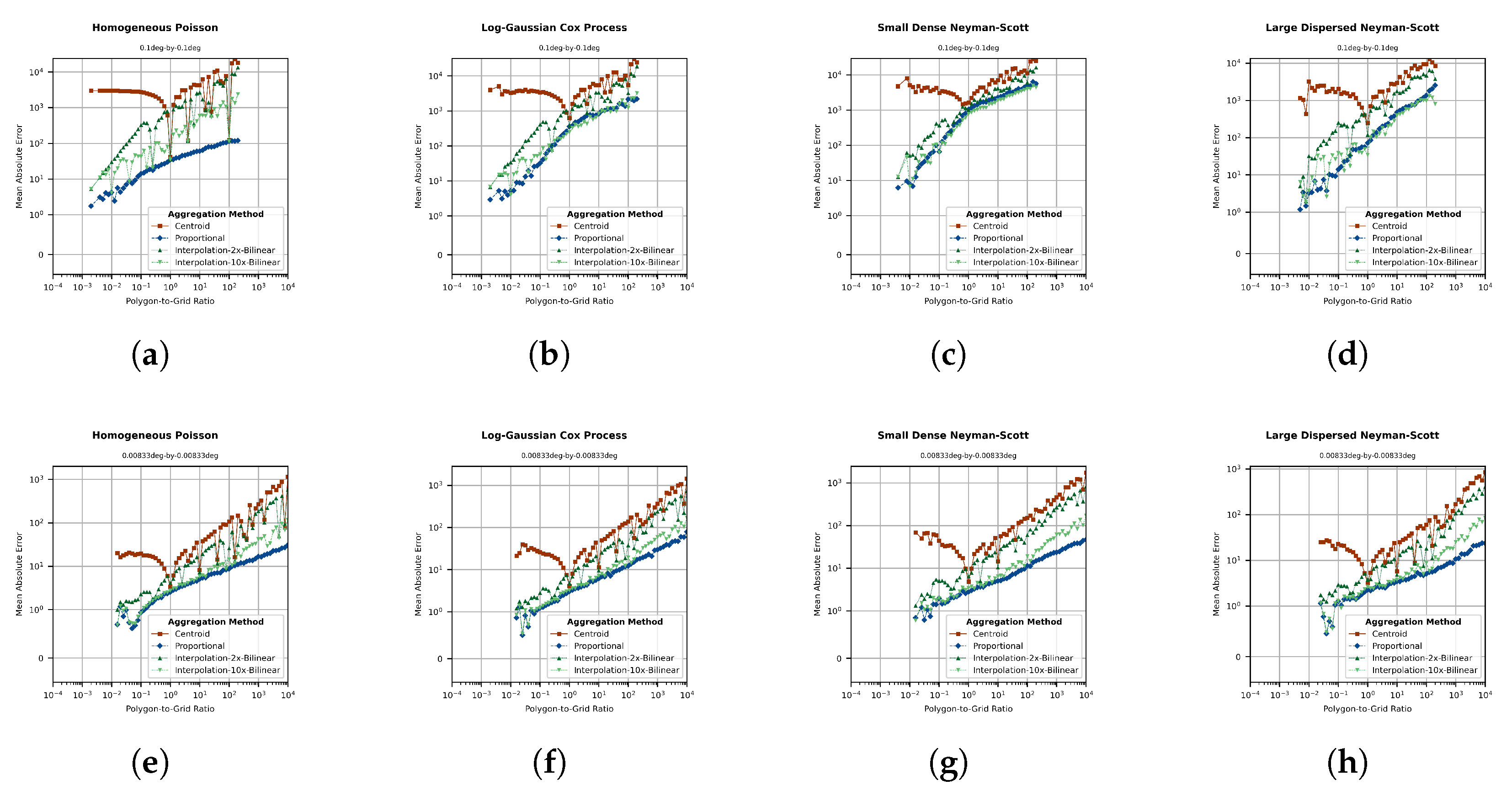
For our synthetic data experiments, we include results from two additional metrics. In
Figure A4, we show the Mean Absolute Error (MAE) for all eight synthetic data cases. We observe that the MAE for centroid aggregation is visibly larger for PGR
than the MAE for the other three aggregation methods (proportional, Interpolation-2×-Bilinear, and Interpolation-10×-Bilinear. In
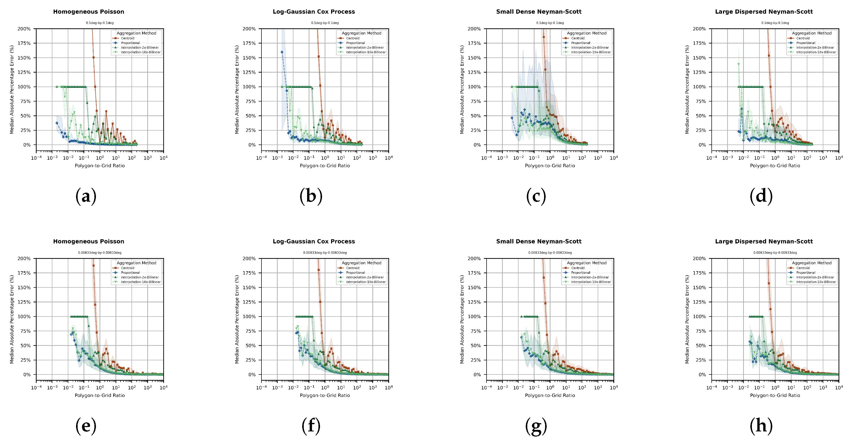
Figure A5, we show the Median Absolute Percentage Error, which also shows poor performance for centroid aggregation when PGR
. We also see that the median percentage error generally decreases as PGR
r increases, with a larger median error and interquartile range (IQR) for the larger grid cell size and smaller median error and IQR for the smaller grid cell size. This highlights expected error as a function of
r and
c for point process data generated from a variety of distributions with different parameters.
Figure A4.
We see that the centroid allocation method has visibly larger Mean Absolute Error as compared to the other three aggregation methods when PGR . Subfigures (a–d) reflect 0.1°-by-0.1°grid cell resolution and subfigures (e–h) reflect 0.00833°-by-0.00833°grid cell resolution.
Figure A4.
We see that the centroid allocation method has visibly larger Mean Absolute Error as compared to the other three aggregation methods when PGR . Subfigures (a–d) reflect 0.1°-by-0.1°grid cell resolution and subfigures (e–h) reflect 0.00833°-by-0.00833°grid cell resolution.
Figure A5.
The median percentage error generally decreases as PGR r increases, with a larger median error and IQR for the larger grid cell size and smaller median error and IGR for the smaller grid cell size. Subfigures (a–d) reflect 0.1°-by-0.1°grid cell resolution and subfigures (e–h) reflect 0.00833°-by-0.00833°grid cell resolution.
Figure A5.
The median percentage error generally decreases as PGR r increases, with a larger median error and IQR for the larger grid cell size and smaller median error and IGR for the smaller grid cell size. Subfigures (a–d) reflect 0.1°-by-0.1°grid cell resolution and subfigures (e–h) reflect 0.00833°-by-0.00833°grid cell resolution.
Appendix A.6. Best Method Comparison
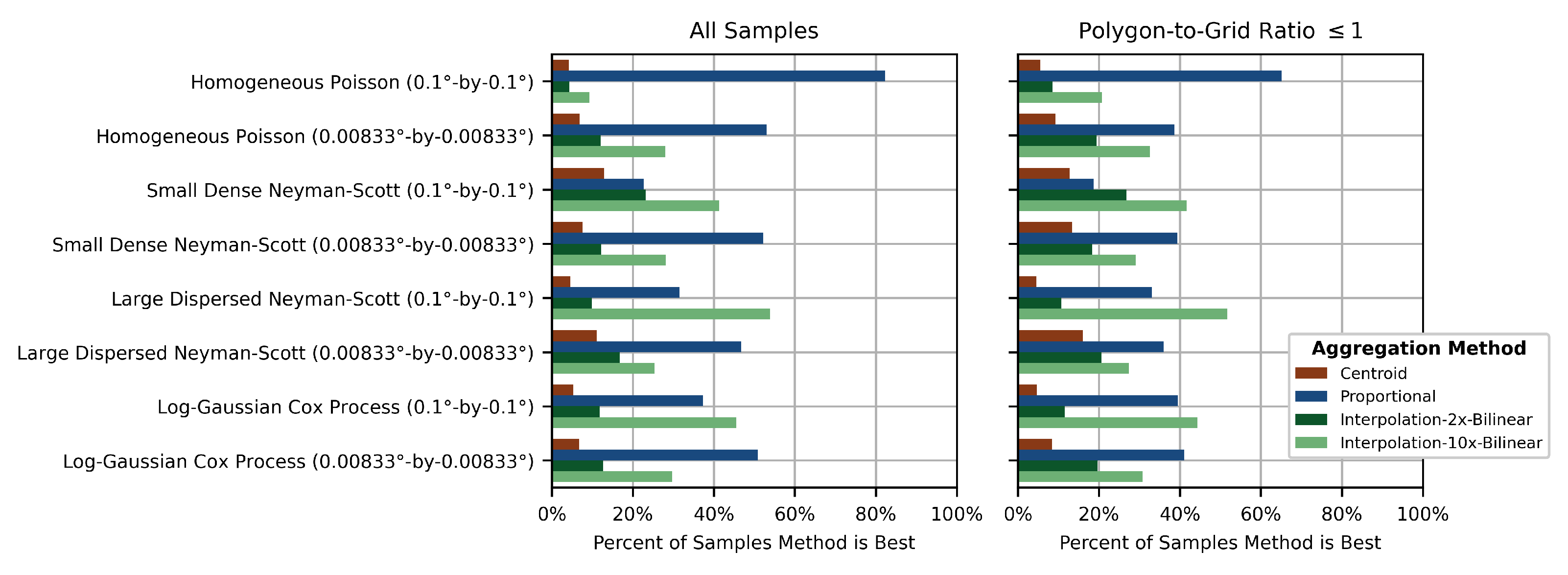
For each sample , we first evaluate which of the four methods is the best method based on the lowest absolute percentage error for each sample. We call R the set of all PGRs r across all samples, and denotes the subset of R containing only the PGRs .
We then define
as the aggregate proportion of success across all samples
r for Method
as
We also define
as the aggregate proportion of success across all samples
for Method
as
We observe that across all of our sampled data, regardless of the data distribution and grid cell size, c and for all methods k, which suggests that there always exists a non-negligible number of samples in which each method is correspondingly the best method. While generally the centroid method is universally the highest error, there are still a non-negligible number of individual samples in which it has lower error than the other methods.
Figure A6.
Comparison of the percentage of individual samples in which each aggregation method is best across all synthetic data distributions and grid cell sizes. Regardless of the PGR r and grid cell size c, there exist samples for which each method is the best method. (Left) We observe this across all samples. (Right) We also observe this across the subset of samples for which the PGR .
Figure A6.
Comparison of the percentage of individual samples in which each aggregation method is best across all synthetic data distributions and grid cell sizes. Regardless of the PGR r and grid cell size c, there exist samples for which each method is the best method. (Left) We observe this across all samples. (Right) We also observe this across the subset of samples for which the PGR .
References
- Wicks, T.E.; Smith, G.M.; Curran, P.J. Polygon-based aggregation of remotely sensed data for regional ecological analyses. Int. J. Appl. Earth Obs. Geoinf. 2002, 4, 161–173. [Google Scholar] [CrossRef]
- Lloyd, C.T.; Sorichetta, A.; Tatem, A.J. High resolution global gridded data for use in population studies. Sci. Data 2017, 4, 170001. [Google Scholar] [CrossRef]
- Mastrantonas, N.; Furnari, L.; Magnusson, L.; Senatore, A.; Mendicino, G.; Pappenberger, F.; Matschullat, J. Forecasting extreme precipitation in the central Mediterranean: Changes in predictors’ strength with prediction lead time. Meteorol. Appl. 2022, 29, e2101. [Google Scholar] [CrossRef]
- Auffhammer, M.; Hsiang, S.M.; Schlenker, W.; Sobel, A. Using Weather Data and Climate Model Output in Economic Analyses of Climate Change. Rev. Environ. Econ. Policy 2013, 7, 181–198. [Google Scholar] [CrossRef]
- Carleton, T.A.; Jina, A.; Delgado, M.T.; Greenstone, M.; Houser, T.; Hsiang, S.M.; Hultgren, A.; Kopp, R.E. Estimating a social cost of carbon for global energy consumption. Nature 2021, 598, 308–314. [Google Scholar] [CrossRef] [PubMed]
- Hsiang, S.; Kopp, R.; Jina, A.; Rising, J.; Delgado, M.; Mohan, S.; Rasmussen, D.J.; Muir-Wood, R.; Wilson, P.; Oppenheimer, M.; et al. Estimating economic damage from climate change in the United States. Science 2017, 356, 1362–1369. [Google Scholar] [CrossRef]
- Schlenker, W.; Roberts, M.J. Nonlinear temperature effects indicate severe damages to U.S. crop yields under climate change. Proc. Natl. Acad. Sci. USA 2009, 106, 15594–15598. [Google Scholar] [CrossRef]
- Goodchild, M.F.; Siu-Ngan Lam, N. Areal interpolation: A variant of the traditional spatial problem. Geo-Processing 1980, 1, 297–312. [Google Scholar]
- Krivoruchko, K.; Gribov, A.; Krause, E. Multivariate Areal Interpolation for Continuous and Count Data. Procedia Environ. Sci. 2011, 3, 14–19. [Google Scholar] [CrossRef]
- What is areal interpolation? —ArcMap | Documentation. Available online: https://desktop.arcgis.com/en/arcmap/latest/extensions/geostatistical-analyst/what-is-areal-interpolation.htm (accessed on 19 March 2026).
- Tobler, W.R. Smooth Pycnophylactic Interpolation for Geographical Regions. J. Am. Stat. Assoc. 1979, 74, 519–530. [Google Scholar] [CrossRef]
- Eicher, C.L.; Brewer, C.A. Dasymetric Mapping and Areal Interpolation: Implementation and Evaluation. Cartogr. Geogr. Inf. Sci. 2001, 28, 125–138. [Google Scholar] [CrossRef]
- Bondarenko, M.; Priyatikanto, R.; Tejedor-Garavito, N.; Zhang, W.; McKeen, T.; Cunningham, A.; Woods, T.; Hilton, J.; Cihan, D.; Nosatiuk, B.; et al. The Spatial Distribution of Population in 2015–2030 at a Resolution of 30 arc (Approximately 1 km at the Equator) R2025A Version v1; University of Southampton: Southampton, UK, 2025. [Google Scholar] [CrossRef]
- European Commission, JRC. EDGAR (Emissions Database for Global Atmospheric Research) Community GHG Database, a Collaboration Between the European Commission, Joint Research Centre (JRC), the International Energy Agency (IEA), and Comprising IEA-EDGAR CO2, EDGAR CH4, EDGAR N2O, EDGAR F-GASES, 2025. Available online: https://edgar.jrc.ec.europa.eu/dataset_ghg2025 (accessed on 19 March 2026).
- Hersbach, H.; Bell, B.; Berrisford, P.; Biavati, G.; Horanyi, A.; Munoz Sabater, J.; Nicolas, J.; Peubey, C.; Radu, R.; Rozum, I.; et al. ERA5 Hourly Data on Single Levels from 1940 to Present; Copernicus Institute: Utrecht, The Netherlands, 2023. [Google Scholar] [CrossRef]
- GADM. Database of Global Administrative Areas, 2025. Available online: https://gadm.org/ (accessed on 19 March 2026).
- Schiavina, M.; Moreno-Monroy, A.; Maffenini, L.; Veneri, P. GHS-FUA R2019A—GHS Functional Urban Areas, Derived from GHS-UCDB R2019A; European Commision: Bruxelles, Belgium, 2015. [Google Scholar] [CrossRef]
- Moreno-Monroy, A.; Schiavina, M.; Veneri, P. Metropolitan areas in the world. Delineation and population trends. J. Urban Econ. 2020, 125, 103242. [Google Scholar] [CrossRef]
- Diggle, P.J.; Besag, J.; Gleaves, J.T. Statistical Analysis of Spatial Point Patterns by Means of Distance Methods. Biometrics 1976, 32, 659–667. [Google Scholar] [CrossRef]
- Almquist, Z.; Butts, C.T. Point process models for household distributions within small areal units. Demogr. Res. 2012, 26, 593–632. [Google Scholar] [CrossRef]
- Neyman, J.; Scott, E.L. Statistical Approach to Problems of Cosmology. J. R. Stat. Soc. Ser. B Methodol. 1958, 20, 1–29. [Google Scholar] [CrossRef]
- Neyman, J.; Scott, E.L. Stochastic Models of Population Dynamics. Science 1959, 130, 303–308. [Google Scholar] [CrossRef] [PubMed]
- Beneš, V.; Bodlák, K.; Møller, J.; Waagepetersen, R. A Case Study on Point Process Modelling in Disease Mapping. Image Anal. Stereol. 2005, 24, 159–168. [Google Scholar] [CrossRef]
- Waagepetersen, R.P. An Estimating Function Approach to Inference for Inhomogeneous Neyman–Scott Processes. Biometrics 2007, 63, 252–258. [Google Scholar] [CrossRef]
- Gratzer, G.; Waagepetersen, R.P. Seed Dispersal, Microsites or Competition—What Drives Gap Regeneration in an Old-Growth Forest? An Application of Spatial Point Process Modelling. Forests 2018, 9, 230. [Google Scholar] [CrossRef]
- Park, J.; Chang, W.; Choi, B. An interaction Neyman–Scott point process model for coronavirus disease-19. Spat. Stat. 2022, 47, 100561. [Google Scholar] [CrossRef]
- Møller, J.; Syversveen, A.R.; Waagepetersen, R.P. Log Gaussian Cox Processes. Scand. J. Stat. 1998, 25, 451–482. [Google Scholar] [CrossRef]
- Li, Y.; Brown, P.; Gesink, D.; Rue, H. Log Gaussian Cox processes and spatially aggregated disease incidence data. Stat. Methods Med. Res. 2012, 21, 479–507. [Google Scholar] [CrossRef]
- Diggle, P.J.; Moraga, P.; Rowlingson, B.; Taylor, B.M. Spatial and Spatio-Temporal Log-Gaussian Cox Processes: Extending the Geostatistical Paradigm. Statist. Sci. 2013, 28, 542–563. [Google Scholar] [CrossRef]
- McCoy, D.; Goulet-Scott, B.; Meng, W.; Atahan, B.; Kiros, H.; Nishino, M.; Kartesz, J. A dataset of 5 million city trees from 63 US cities: Species, location, nativity status, health, and more. bioRxiv 2022. [Google Scholar] [CrossRef]
- Moran, P.A.P. Notes on Continuous Stochastic Phenomena. Biometrika 1950, 37, 17–23. [Google Scholar] [CrossRef] [PubMed]
- Perry, M. Rasterstats Python Package, 2024. Available online: https://pythonhosted.org/rasterstats/ (accessed on 19 March 2026).
- Baston, D. Exactextract, 2025. Original-Date: 2018-06-12T19:15:57Z. Available online: https://pypi.org/project/exactextract/ (accessed on 19 March 2026).
- Project Geospatial. FOSS4G NA 2024—Speeding Up Raster/Vector Zonal Analysis with Exactextract–Dan Baston, 2025. Available online: https://www.youtube.com/watch?v=er9G1DLNuoc (accessed on 19 March 2026).
- Rasterio: Access to Geospatial Raster Data—Rasterio 1.4.4 Documentation. Available online: https://rasterio.readthedocs.io/en/stable/ (accessed on 19 March 2026).
Figure 1.
Illustrative extreme-case example showing a potential limitation associated with the centroid allocation method. While uniformly distributed underlying point data would result in a ground truth polygon value of 96, the centroid method would estimate a value of 0 for this polygon because the polygon is just small enough that it does not intersect with any of the grid cell centroids.
Figure 1.
Illustrative extreme-case example showing a potential limitation associated with the centroid allocation method. While uniformly distributed underlying point data would result in a ground truth polygon value of 96, the centroid method would estimate a value of 0 for this polygon because the polygon is just small enough that it does not intersect with any of the grid cell centroids.
Figure 2.
Real-world example comparing population, emissions, and total snowfall raster data that exist at different grid cell resolutions. These data are considered in comparison with two different geospatial boundaries of varying size: a larger boundary representing the contiguous United States, and a significantly smaller boundary representing the island of Manhattan in New York City. For each such comparison, we compute metrics such as a PGR of the polygon area to the grid cell area, the number of all-touched grid cells intersecting the polygon boundary, and the number of grid cells whose centroid falls within the polygon boundary. We can visually observe the differences in grid-to-polygon allocation in cases where there are large polygons relative to the grid cell size and small polygons relative to the grid cell size. The PGR and grid cell size are key determinants of aggregation method expected performance.
Figure 2.
Real-world example comparing population, emissions, and total snowfall raster data that exist at different grid cell resolutions. These data are considered in comparison with two different geospatial boundaries of varying size: a larger boundary representing the contiguous United States, and a significantly smaller boundary representing the island of Manhattan in New York City. For each such comparison, we compute metrics such as a PGR of the polygon area to the grid cell area, the number of all-touched grid cells intersecting the polygon boundary, and the number of grid cells whose centroid falls within the polygon boundary. We can visually observe the differences in grid-to-polygon allocation in cases where there are large polygons relative to the grid cell size and small polygons relative to the grid cell size. The PGR and grid cell size are key determinants of aggregation method expected performance.
Figure 3.
Median absolute percentage differences as a function of PGR for real-world gridded datasets. These differences are considered across each of our four sets of boundaries. In (a) we show the WorldPop population data comparison, with a 30arcsec-by-30arcsec spatial resolution corresponding to approximately a 1km-by-1km grid cell. In (b) we show the EDGAR gridded emissions data comparison, with a 0.1°-by-0.1°spatial resolution corresponding to approximately an 11km-by-11km grid cell. These data show that as the PGR increases, the percentage difference between centroid and proportional aggregation approach 0%, suggesting that both methods estimate the same value; however, for smaller PGRs and especially PGR ≤ 1, there could be differences up to 100% between the estimates from the two methods.
Figure 3.
Median absolute percentage differences as a function of PGR for real-world gridded datasets. These differences are considered across each of our four sets of boundaries. In (a) we show the WorldPop population data comparison, with a 30arcsec-by-30arcsec spatial resolution corresponding to approximately a 1km-by-1km grid cell. In (b) we show the EDGAR gridded emissions data comparison, with a 0.1°-by-0.1°spatial resolution corresponding to approximately an 11km-by-11km grid cell. These data show that as the PGR increases, the percentage difference between centroid and proportional aggregation approach 0%, suggesting that both methods estimate the same value; however, for smaller PGRs and especially PGR ≤ 1, there could be differences up to 100% between the estimates from the two methods.
Figure 4.
Synthetic point process data generated to be representative of real-world ground truth point process data. Based on varying sets of underlying parameters, the ground truth points generated from homogeneous Poisson are shown in (a), Log-Gaussian Cox process in (b), Large Dispersed Neyman–Scott in (c), and Small Dense Neyman–Scott in (d).
Figure 4.
Synthetic point process data generated to be representative of real-world ground truth point process data. Based on varying sets of underlying parameters, the ground truth points generated from homogeneous Poisson are shown in (a), Log-Gaussian Cox process in (b), Large Dispersed Neyman–Scott in (c), and Small Dense Neyman–Scott in (d).
Figure 5.
Example rasterization process for synthetic point process data. Using the Large Dispersed Neyman–Scott point process data in (a), we rasterize the data. In (b) we show the resulting raster using the larger grid cell size of 0.1°-by-0.1°. In (c) we show the resulting raster using the smaller grid cell size of 0.00833°-by-0.00833°. We observe that more of the variance in the ground truth point process data distribution are captured in the raster with the smaller grid cell size, whereas the larger grid cells tend to lose some of that variance and suggest a more uniform distribution in the underlying point process data than is actually present.
Figure 5.
Example rasterization process for synthetic point process data. Using the Large Dispersed Neyman–Scott point process data in (a), we rasterize the data. In (b) we show the resulting raster using the larger grid cell size of 0.1°-by-0.1°. In (c) we show the resulting raster using the smaller grid cell size of 0.00833°-by-0.00833°. We observe that more of the variance in the ground truth point process data distribution are captured in the raster with the smaller grid cell size, whereas the larger grid cells tend to lose some of that variance and suggest a more uniform distribution in the underlying point process data than is actually present.
Figure 6.
Comparison of Weighted Absolute Percentage Error as a function of PGR by aggregation method for each synthetic data distribution. Subfigures (a–d) reflect 0.1°-by-0.1°grid cell resolution and subfigures (e–h) reflect 0.00833°-by-0.00833°grid cell resolution. The centroid allocation method shows far greater WAPE for PGR than the other three aggregation methods, suggesting that there could be far more severe consequences in using centroid aggregation in cases where the polygon is smaller than the grid cell size.
Figure 6.
Comparison of Weighted Absolute Percentage Error as a function of PGR by aggregation method for each synthetic data distribution. Subfigures (a–d) reflect 0.1°-by-0.1°grid cell resolution and subfigures (e–h) reflect 0.00833°-by-0.00833°grid cell resolution. The centroid allocation method shows far greater WAPE for PGR than the other three aggregation methods, suggesting that there could be far more severe consequences in using centroid aggregation in cases where the polygon is smaller than the grid cell size.
Figure 7.
Comparison of consequence factors by aggregation method for each synthetic data distribution. Subfigures (a–d) reflect 0.1°-by-0.1°grid cell resolution and subfigures (e–h) reflect 0.00833°-by-0.00833°grid cell resolution. We see that the CF for the centroid aggregation method is far greater than the other three methods for PGR , suggesting that there is far greater consequence of choosing the centroid method and being wrong about that choice of aggregation method than choosing one of the other three aggregation methods and being wrong.
Figure 7.
Comparison of consequence factors by aggregation method for each synthetic data distribution. Subfigures (a–d) reflect 0.1°-by-0.1°grid cell resolution and subfigures (e–h) reflect 0.00833°-by-0.00833°grid cell resolution. We see that the CF for the centroid aggregation method is far greater than the other three methods for PGR , suggesting that there is far greater consequence of choosing the centroid method and being wrong about that choice of aggregation method than choosing one of the other three aggregation methods and being wrong.
Table 1.
Real-world differences between centroid and proportional aggregation across datasets and boundary types. For each combination of dataset and real-world polygon boundary category (country-, county-, or city-level), we provide the median absolute percentage difference between estimates derived from each aggregation method. We also include the percentage of polygons in the boundary set that demonstrate greater than 10% and greater than 50% absolute percentage difference between the two aggregation methods. We finally include the largest absolute difference across the boundary set for each dataset, reported in the native units of the corresponding raster dataset.
Table 1.
Real-world differences between centroid and proportional aggregation across datasets and boundary types. For each combination of dataset and real-world polygon boundary category (country-, county-, or city-level), we provide the median absolute percentage difference between estimates derived from each aggregation method. We also include the percentage of polygons in the boundary set that demonstrate greater than 10% and greater than 50% absolute percentage difference between the two aggregation methods. We finally include the largest absolute difference across the boundary set for each dataset, reported in the native units of the corresponding raster dataset.
| Dataset | Grid Cell Resolution | Boundary Category | Median Abs. Perc. Diff. | Polygons >10% Perc. Diff. | Polygons >50% Perc. Diff. | Largest Abs. Diff. |
|---|
| Population [13] | -by- | Country | 0.2% | 4.3% | 0.8% | 776,979.94 |
| County | 0.6% | 4.0% | 0.5% | 123,762.71 |
| City | 0.9% | 4.6% | 0.1% | 121,260.79 |
| GHG Emissions (tonnes) [14] | 0.1°-by-0.1° | Country | 1.0% | 26.2% | 12.9% | 19,684,990.42 |
| County | 14.8% | 59.2% | 24.1% | 23,908,073.04 |
| City | 100.0% | 85.1% | 60.5% | 1,259,003.74 |
| Snowfall (mm of water equivalent) [15] | 0.25°-by-0.25° | Country | 0.4% | 9.5% | 3.4% | 87,817.50 |
| County | 12.6% | 55.7% | 23.8% | 43,872.27 |
| City | 27.5% | 73.5% | 36.0% | 672.79 |
Table 2.
Compute time summary (mean ± standard deviation). The bold times denote the minimum mean durations.
Table 2.
Compute time summary (mean ± standard deviation). The bold times denote the minimum mean durations.
| Aggregation Method | Resolution | Duration (s) |
|---|
| Centroid | 0.1°-by-0.1° | 591.5 ± 1.2 |
| Proportional | 0.1°-by-0.1° | 407.5 ± 1.9 |
| Interpolation-2×-Bilinear | 0.1°-by-0.1° | 583.2 ± 4.0 |
| Interpolation-10×-Bilinear | 0.1°-by-0.1° | 559.5 ± 7.5 |
| Centroid | 0.00833°-by-0.00833° | 554.3 ± 16.5 |
| Proportional | 0.00833°-by-0.00833° | 407.8 ± 1.0 |
| Interpolation-2×-Bilinear | 0.00833°-by-0.00833° | 564.6 ± 16.8 |
| Interpolation-10×-Bilinear | 0.00833°-by-0.00833° | 974.5 ± 23.3 |
| Disclaimer/Publisher’s Note: The statements, opinions and data contained in all publications are solely those of the individual author(s) and contributor(s) and not of MDPI and/or the editor(s). MDPI and/or the editor(s) disclaim responsibility for any injury to people or property resulting from any ideas, methods, instructions or products referred to in the content. |
© 2026 by the authors. Published by MDPI on behalf of the International Society for Photogrammetry and Remote Sensing. Licensee MDPI, Basel, Switzerland. This article is an open access article distributed under the terms and conditions of the Creative Commons Attribution (CC BY) license.