


Abstract
Accurate and timely extraction of land–water boundaries is essential for water resources management, flood monitoring, and wetland conservation. This study proposes a method for extracting land–water boundaries from unmanned aerial vehicle (UAV)-borne bathymetric light detection and ranging (LiDAR) point clouds. First, land point clouds are projected onto a reference plane constructed by fitting water surface points. Next, an alpha-shape algorithm extracts the boundary of these projected points. A combined algorithm of periodic curvature adaptive exponential tension spline interpolation and Savitzky–Golay (SG) filtering is then applied for secondary smoothing to generate the land boundary curve. Finally, curve segments adjacent to water surface points are identified as the land–water boundary. Experimental results show that, compared with manual extraction, the method yielded a root mean square error (RMSE) of 0.118 m at Danjiangkou Reservoir (main test area) and 0.184 m against independent real-time kinematic (RTK) measurements at Suzhou Reservoir. This demonstrates that UAV-borne bathymetric LiDAR meets the requirements for refined boundary extraction, and the proposed secondary smoothing algorithm successfully balances accuracy and smoothness to accurately reflect natural boundary morphology.
1. Introduction
Land–water boundaries distinguish land from water bodies and exhibit diverse morphologies, including coastal, lacustrine, and fluvial shorelines [1,2]. Their spatial evolution is closely related to ecological security, coastal management, and resource development. Climate change, sea level rise, and increasing human activities have significantly altered shoreline morphology, causing erosion, retreat, and sedimentation in many coastal regions [3,4,5]. Therefore, accurate land–water boundary data offer significant utility in domains such as water resource management, flood risk assessment, shoreline erosion monitoring, and urban planning. For water resource management authorities, multi-temporal boundary data can be utilized to dynamically monitor shifts in riverine and lacustrine shorelines, variations in reservoir capacities, and the extent of bank erosion. In terms of urban planning, high-precision boundary data offer baseline geographic information for delineating urban blue lines (water protection zones), regulating waterfront development, and inspecting illegal encroachments. Therefore, acquiring well-timed and precise land–water boundaries is of profound relevance [6,7,8,9].
Traditional shoreline measurement techniques, such as terrestrial surveying, can be used to track shoreline changes, but they have limitations such as limited spatial resolution, high interpretation costs, and long processing times [10,11]. With the advancement of remote sensing technology, optical and synthetic aperture radar (SAR) imagery have been widely used for shoreline extraction due to their broad spatial coverage. Pardo-Pascual et al. [12] proposed a multistage extraction pipeline using Landsat and Sentinel-2 imagery for subpixel shoreline extraction. Choung and Jo [13] utilized WorldView-2 imagery to compare normalized difference water index and support vector machine (SVM) methods, revealing that SVM yielded superior accuracy in areas with irregular morphologies and shadows, whereas both methods exhibited suboptimal performance in regions with intense shadowing.
In comparison, SAR has all-weather observation capabilities and can effectively replace optical imagery for extracting coastlines in cloudy or nighttime conditions [14,15,16]. However, when the contrast between the ocean and the land is not strong, SAR images suffer from problems such as blurred boundaries, high gray values, and susceptibility to noise interference, making coastline extraction based on SAR images difficult. To address this issue, Wei et al. [17] proposed a land–sea boundary detection method based on a geometric active contour model, which effectively alleviated the problem of blurred coastline boundaries under complex conditions. However, the parameter configuration and the design of the energy functional lack a solid theoretical foundation.
In addition to remote sensing imaging, with the development of airborne laser scanning (ALS) technology, researchers have begun to explore its application in coastline extraction. Xu et al. [18] proposed a new method for shoreline extraction directly from three-dimensional LiDAR point clouds. By optimizing the land boundary using a minimum-cost boundary model, they achieved 92.5% completeness and 90.7% accuracy. Li et al. [19] conducted research on high-precision coastline extraction methods applicable to complex coastal environments, and proposed the Shoreline_veget method, which solved the problems of low coastline extraction accuracy and poor algorithm stability caused by vegetation shading in vegetated sea areas.
Although extensive studies on shoreline extraction using multi-source remote sensing data, including optical imagery, SAR imagery, and airborne LiDAR, are available, these traditional methods rely heavily on heuristic thresholds and empirical parameters. This has led to limited generalization across different regions and hydrological conditions. For example, water-index-based methods such as normalized difference water index (NDWI) and modified normalized difference water index (MNDWI) are highly sensitive to terrain-based variations, mountains, and shadow effects, rendering stable performance in cross-regional or multi-temporal scenarios extremely challenging [20]. In addition, methods associated with fixed elevation stratification and predefined grid resolutions are often unfeasible for ALS datasets with high water levels. The high sensitivity of such methods to specific datasets makes parameters tuned for a particular region impractical to apply in areas with distinct hydrological and topographical characteristics, thereby limiting their generalization capacity [21]. This limitation becomes more pronounced in the extraction of narrow water bodies and small tributaries, where threshold uncertainty can easily translate into fragmented boundaries and edge voids, jeopardizing the complete capture of the extracted shoreline [22].
Compared to traditional two-dimensional remote sensing imagery, the ALS system can directly acquire high-precision three-dimensional terrain information. But traditional airborne platforms are limited by bulky equipment, high flight altitude requirements, restricted point density, and high costs. These constraints render them ill-suited for high-resolution, rapid response, and localized fine-grained shoreline monitoring and lead to insufficient capability for identifying low-tide flats, micro-topographic variations, and complex shorelines [23]. Traditional ALS systems cannot acquire underwater topographic information, while airborne LiDAR bathymetry (ALB) technology has developed rapidly, becoming an important means of integrated land–sea mapping as a result of its high precision, high efficiency, and full-waveform sampling capabilities, and can simultaneously acquire land and underwater topographic data [23,24,25]. Simultaneously, with the advancement of UAV and lightweight sensor technologies, UAV-borne LiDAR bathymetry (UAV-ALB) has been increasingly used for the high-resolution mapping of nearshore and shallow water areas [26]. Its low-altitude operation effectively reduces spot size, achieves centimeter-level resolution and high-density point clouds, improves the ability to identify shallow waters and shoreline microtopography, and enables continuous observation and precise demarcation of the land–sea transition zone [27]. Compared with manned aircraft platforms, UAV platforms have advantages such as high maneuverability, ease of deployment, and cost-effectiveness. These features enable high-precision mapping tasks in areas that are difficult to cover using traditional airborne systems, such as complex shorelines, tidal flats, and islands [28,29,30].
In the UAV-ALB system, the land–water classification information of the point clouds is mainly derived from dual-wavelength lasers (infrared 1064 nm and green 532 nm) and their corresponding full-waveform features, which form the foundation for boundary extraction. Previous studies have indicated that infrared returns tend to saturate on land surfaces but attenuate rapidly on water surfaces and within bodies of water. The saturation characteristic of infrared echoes is widely considered the earliest and most robust criterion for land–water discrimination. Some systems have also attempted to use the 647 nm Raman scattering signal excited by a 532 nm laser to distinguish water bodies; however, this is rarely used in modern lightweight platforms because of system complexity and airborne platform weight requirements. In recent years, by extracting multi-dimensional waveform features of infrared and green lasers (such as amplitude, full width at half maximum, area, and spectral ratio) and combining them with support vector machines or deep learning models, a land–water waveform classification accuracy of 95–99% can be achieved [31].
Misclassification in the research data primarily manifests as water-surface points with strong echoes being labeled as land points. Since these points are located within the water body (away from the shoreline), they do not affect subsequent steps such as boundary extraction. Based on this, a semi-automatic land–water boundary extraction method using UAV-ALB point cloud data is proposed. Leveraging the land–water classification information derived from the UAV-ALB system, the method follows a complete workflow consisting of “reference plane acquisition and elevation normalization—land boundary extraction—two-stage smoothing—land–water boundary extraction”. Its accuracy and feasibility are further validated using representative field-measured datasets. This study focuses on the instantaneous land–water boundary, a primary indicator for airborne LiDAR-based shoreline extraction [18]. Because UAV-ALB point clouds utilize geodetic heights rather than specific tidal datums, the extracted boundaries can be flexibly transformed across diverse vertical datums. The present study aims to provide a highly dynamic land–water boundary measurement approach that can provide novel technical insights for high-resolution nearshore mapping and shoreline monitoring.
2. Methods
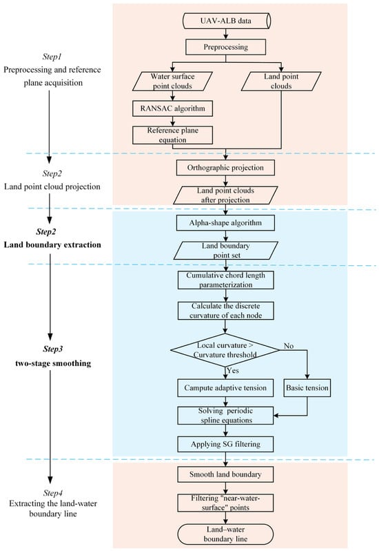
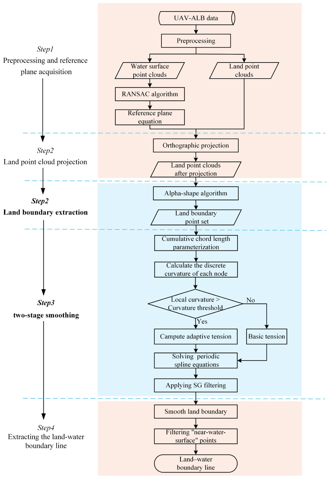
The proposed method for extracting land–water boundaries primarily comprises the following five key modules: (1) UAV-ALB point cloud preprocessing and reference plane acquisition. Preprocessing includes point cloud noise removal and downsampling. Denoising is a routine processing step for UAV-ALB raw point clouds from data acquisition to the generation of final data products, employing a combination of automated and manual methods. Subsequently, the water and land point cloud data are downsampled to reduce data redundancy and improve computational efficiency while preserving terrain features. (2) Projection of land point clouds. To mitigate the impact of complex terrain undulations on boundary extraction, an orthogonal projection method was employed to project the downsampled terrestrial point cloud onto a fitted reference plane. (3) Extraction of land boundary. Based on the projected two-dimensional land point set, the alpha-shape algorithm was employed to extract the land boundary, facilitating detailed representation of landform geometry. (4) Boundary smoothing. As the initial boundary extracted by the alpha-shape algorithm is sensitive to local discrete points and boundary jaggedness, a combination of periodic curvature adaptive exponential tension spline interpolation and SG filtering was adopted for secondary smoothing of the boundary. This improves the smoothness and continuity of the boundary curve. (5) Extraction of the land–water boundary line. The smoothed land boundary curves were filtered, and those adjacent to the water surface point cloud were selected as the final extracted land–water boundary line.
The overall process is shown through a flow diagram (Figure 1).
Figure 1.
Land–water boundary extraction process.
2.1. Reference Plane Acquisition
To reduce the influence of complex terrain on the calculation of the land–water boundary and consider the randomness of water surface waves, water surface point cloud data were extracted from UAV-ALB data, and the water surface equation was fitted using the RANSAC method as the reference plane. The water-surface point cloud was first extracted based on the LAS file classification results of the UAV-ALB data. Subsequently, three points that were noncollinear and had relatively large spacing were randomly selected as the initial fitting point set, and the water-surface plane model was calculated as follows:
where the coefficients were assumed to be normalized; accordingly, denotes the unit normal vector of the plane.
The distances from all remaining water-surface points to the plane were then computed. If the distance was smaller than the threshold, the point was considered lying on the same plane. An excessively large threshold may include too many outliers and reduce the fitting accuracy, whereas an excessively small threshold may result in insufficient inliers and unstable fitting results. The aforementioned steps were repeated if the number of inliers in the current model exceeded the maximum number previously recorded, and the model parameters were updated. The iteration continued until convergence, and the plane model with the most inliers was selected as the final reference plane, P.
The primary purpose of this step is to establish a unified reference datum, thereby providing a stable elevation reference for subsequent land points projection and boundary extraction. Meanwhile, the robustness of RANSAC against outliers helps to suppress the influence of local wave fluctuations and discrete point cloud noise on boundary computation.
2.2. Land Point Clouds Projected onto Reference Plane
After obtaining the reference plane, the land point clouds were projected onto this reference plane so that the land and water data were located on the same reference plane, which facilitated a more accurate calculation of the land–water boundary position. An orthogonal projection method was used to project all land points perpendicular to the reference plane along the direction of the plane’s normal vector.
First, the land point cloud set is extracted based on the classification results as , where . The projection transformation aims to find a point on plane P such that vector is parallel to the plane normal vector . The projection point is calculated as
where scalar t is the signed distance from to plane P. As the normal vector is normalized, it can be simplified to , and the matrix form of the projection transformation can be obtained as follows:
After this transformation, the projected land point set was strictly constrained to the reference plane P, thus completing the normalization of land elevation to the reference plane. The extraction of land boundaries was transformed from a complex 3D spatial search into a 2D planar topological reconstruction problem. This transformation effectively mitigates computational complexity and eliminates the interference of terrain elevation undulations on horizontal boundary localization.
2.3. Land Boundary Extraction via Alpha-Shape Algorithm
After completing the orthogonal projection, the boundaries of the land point clouds were extracted. Because land–water boundaries typically have meandering features, there are obvious depressions. The traditional convex-hull algorithm forcibly closes the depression area, making it difficult to depict the detailed features. Therefore, the alpha-shape algorithm was introduced to reconstruct the geometry of the land projection point set according to the following process.
- (1)
- For the projected land point, was set. Starting from an arbitrary point , another arbitrary point was selected within the neighboring set R defined by a radius of 2α. The center of the circle determined by and was calculated using Equation (4). Considering the concave and convex variations in the landform, the value of α should not be excessively high.where , , and S represents .
- (2)
- The distance L was calculated from all other points within the neighborhood R to the circle center . If all L values are greater than α—meaning no other points lie inside the circumscribed circle—then segment is identified as a boundary line segment; otherwise, it is not.
- (3)
- The previous two steps were repeated for the remaining points within neighborhood R until all points in R were evaluated.
- (4)
- The above procedure was repeated for the remaining points in until all points in were processed.
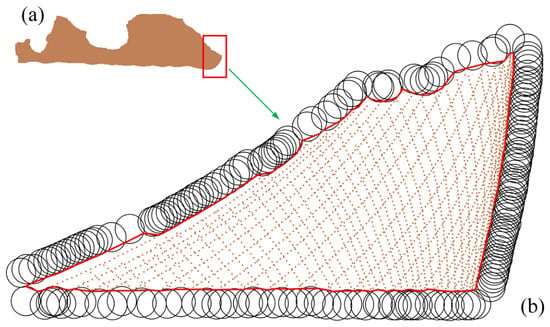
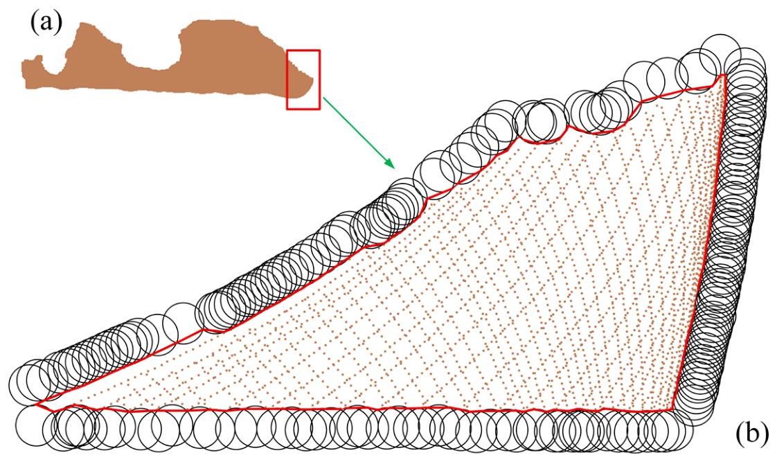
As shown in Figure 2a, a portion of the land point cloud data within the experimental area was selected. Figure 2b presents the boundary extraction process based on the rolling-circle concept of the alpha-shape algorithm, through which local concavities and detailed shoreline features can be effectively captured to represent the true geometric morphology of complex shorelines.
Figure 2.
Schematic diagram of boundary extraction using the alpha-shape algorithm. (a) Land point clouds from a portion of the experimental area. (b) Boundary extraction within the boxed region in (a). The black circles indicate rolling circles with a radius of α, and the red line represents the extracted boundary.
2.4. Boundary Smoothing
The land boundary point set extracted using the alpha-shape algorithm describes the land contour in the form of ordered discrete points. To extract a smooth and continuous land–water boundary that conformed to natural boundary features, a discrete land boundary point set was reconstructed using a two-stage smoothing approach that combined periodic curvature adaptive exponential tension spline interpolation with SG filtering. This approach yields a continuous and smooth land–water boundary that preserves terrain detail.
2.4.1. Periodic Curvature Adaptive Exponential Tension Spline Interpolation
Suppose that the closed boundary extracted by alpha-shape consists of N ordered two-dimensional nodes, , and use the periodic index . To reduce the impact of uneven node spacing on the interpolation results, cumulative chord length parameterization based on Euclidean distance is adopted. The Euclidean distance between adjacent nodes is defined as:
Then the total chord length L of the closed boundary, the normalized cumulative chord length parameter , and the parameter length of the i-th interval are:
This cumulative chord-length parameterization method avoids the distortion caused by the uniform parameterization of non-uniform point sets, making the interpolated curve geometrically closer to the original point-set contour. To adaptively adjust the spline tension constraint based on local geometric complexity, the discrete curvature is first calculated using three adjacent nodes. The discrete curvature at node is:
By averaging the nodal curvature at three points and further calculating the interval curvature between adjacent nodes, the interference of discrete fluctuations on tension regulation can be reduced. The interval curvature is:
The tension parameters of the i-th interval are determined adaptively based on the interval curvature:
where is the base tension, is the curvature threshold, k is the tension enhancement coefficient, and is the upper limit of the extreme tension. When , the tension remains at ; when , the tension increases with increasing curvature, imposing a stronger constraint on this region. Define a local normalization parameter for the i-th interval :
For any planar coordinate component , let denote the second derivative of node with respect to the global parameter t. Combining the interpolation condition , at both ends of the interval and the second derivative condition , , the exponential tension spline expression for the i-th segment is:
In this expression, the tension parameter directly participates in the construction of the piecewise curve, thus ensuring the mathematical consistency between the tension control equation and the curve expression. When approaches 0, the tension spline approximates a classical cubic spline under limiting conditions. As gradually increases, the effect of the hyperbolic function correction term weakens, and the local curve gradually tends towards piecewise linear interpolation. Therefore, increasing the tension in high-curvature sections can suppress overshoot and oscillations, whereas maintaining a lower tension in relatively smooth sections helps preserve the overall smoothness of the curve.
Since the land boundary to be sought is a closed boundary, the same periodic continuity condition as that for the internal nodes is applied to the first and last nodes:
Therefore, the resulting closed curve satisfies positional, first-order derivative, and second-order derivative continuity at the connection points, i.e., it possesses strict periodicity continuity. To solve for the nodal second-order derivative , the parametric slope of the i-th interval and the tension correlation coefficient are defined as:
Based on the condition that adjacent spline intervals satisfy the first derivative continuity condition at the common node , the nodal governing equations can be obtained.
By establishing the above equations using periodic indexing for all N nodes, a system of cyclic linear equations relating to can be obtained. By solving for the X and Y coordinate components separately, obtaining the second derivatives of each node, and substituting them into the piecewise spline expression, a complete two-dimensional spline curve can be obtained.
2.4.2. Secondary Smoothing Using SG Filtering
For the discrete land boundary point set extracted by the alpha-shape algorithm, curve fitting was performed using periodic curvature adaptive exponential tension spline interpolation to transform the discrete data into a curved shape for expression. This step ensures that the curve accurately passes through all the original boundary points and satisfies the continuity of the second derivative at the connection points, thus initially yielding a smooth curve that is locally resistant to oscillation. However, because the input land boundary point set inevitably contains noise, the obtained curve includes some “spur” parts. Therefore, SG filtering can be used for secondary smoothing [32].
Taking the equally spaced curve points generated by the periodic curvature adaptive exponential tension spline curve as input, SG filtering was applied separately to the resulting X and Y coordinate sequences. Using the Y coordinate as an example, within a sliding window of length 2m + 1, an n-th order polynomial is used to fit the window center point i and its neighborhood data :
where a denotes the relative position parameter with respect to the center of the moving window. A window size determines the smoothness of the filter. The larger the window, the smoother the filtering result, but detailed features may be lost. The polynomial order determines the ability to fit local shape changes in the curve. The higher the order, the better the preservation of local geometric features of the curve, such as curvature changes and inflection points. However, excessively high orders may lead to overfitting.
Based on the least squares principle, the coefficient vector is determined by minimizing the sum of squared residuals within the window.
Through matrix operations, the filtered value is obtained as the smoothed value at the window center i, which corresponds to evaluating the fitted polynomial at the central position a = 0:
Therefore, can be expressed as a linear combination of the original window data :
Compared with conventional smoothing methods, such as mean filtering or Gaussian filtering, SG filtering can better preserve the local geometric changes in the signal, thereby effectively suppressing noise while avoiding the blurring of critical inflection points and concave–convex features along the boundary.
2.5. Identification of Land–Water Boundary
Smooth land boundary curves were obtained using the process outlined in Section 2.4. Then, the nearest neighbor query was performed using KD-Tree to select the land boundary curves adjacent to the water surface as the land–water boundary.
First, a KD-Tree index was constructed from the water surface point cloud located on the reference plane. For each endpoint of the land boundary curve, the nearest point in the water-surface point cloud was quickly queried using , and the minimum distance was calculated as . Subsequently, a distance threshold was defined for “near-water surface,” and points with a distance smaller than this threshold were considered “near-water surface” points. Specifically, if , the endpoint is classified as a “near-water surface” point; conversely, if , it is classified as a “non-near-water-surface” point. The classification results for the two endpoints were examined for each line segment of the land boundary curve. A segment was retained only if both endpoints were classified as “near-water-surface” points; otherwise, they were filtered out. The assembly of all retained segments constituted the final extracted land–water boundary.
3. Experiments
3.1. Study Area and Experimental Equipment
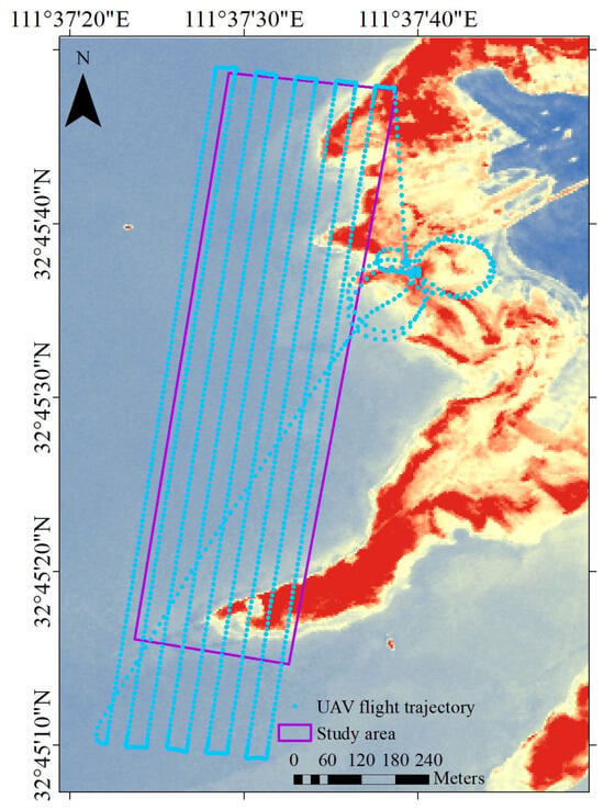
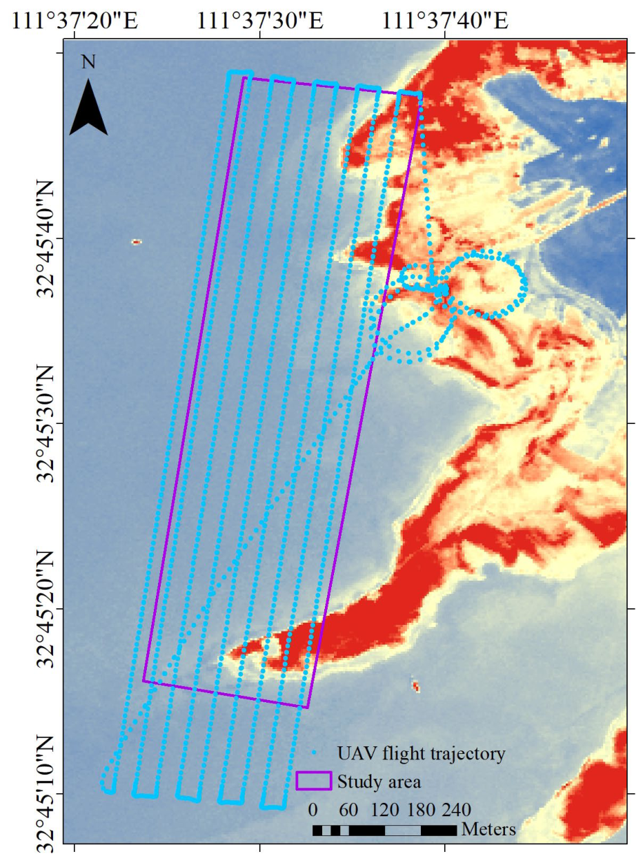
The experimental area was located at Danjiangkou Reservoir, Henan Province. The data size was 494.32 MB with 34,788,743 points. The x coordinates ranged from 558,272.953 to 558,794.162, while the y coordinates ranged from 3,625,449.270 to 3,626,730.618, covering an area of approximately 391,555 m2. The study area features a combined artificial and natural inland reservoir environment, characterized by exposed soil slopes, local rocky shoreline segments, and areas with varying degrees of vegetation cover. An overview of the study area and the flight trajectory is shown in Figure 3.
Figure 3.
Overview of the study area. Flight trajectory (blue) overlaid on Gaofen-2 satellite imagery of the study area (purple).
The data were acquired using the Mapper20KU UAV-ALB system, developed by the Shanghai Institute of Optics and Fine Mechanics, Chinese Academy of Sciences (Shanghai, China). The system features full-waveform recording, multi-return detection, and strong land–water waveform discrimination capabilities [25]. The system specifications are summarized in Table 1.
Table 1.
UAV-ALB sensor and system specifications.
Based on the land–water classification information provided by the UAV-ALB system, the land–water boundary was extracted from the UAV-ALB point cloud using C++ programming, following the methods described in Section 2. The procedure is outlined below.
3.2. Stage 1: Reference Plane Acquisition and Elevation Normalization
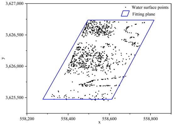
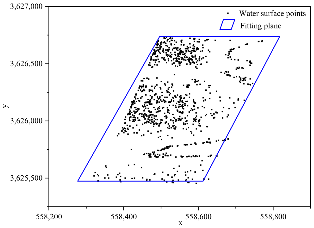
After manual outlier removal and voxel downsampling, the land and water surface point clouds contained 450,564 and 2,614,111 points, respectively, with average point spacings of 0.185 m and 0.189 m. The voxel size was set to 0.3 m to preserve shoreline integrity and local geometric features. The RANSAC algorithm was employed to extract a sufficient number of points and derive an optimal water-surface equation. This ensured an accurately fitted reference plane, onto which the land point clouds were subsequently orthogonally projected (Figure 4).
Figure 4.
RANSAC fitting plane. Water surface plane (blue) fitted to water surface points (black).
3.3. Stage 2: Land Boundary Extraction
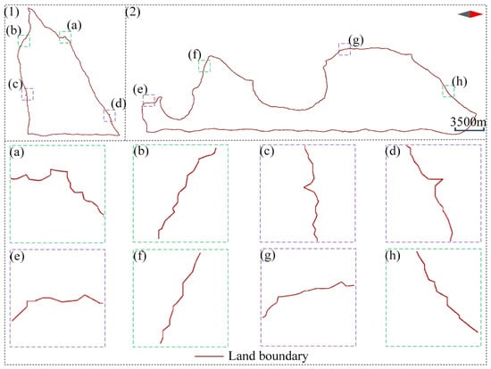
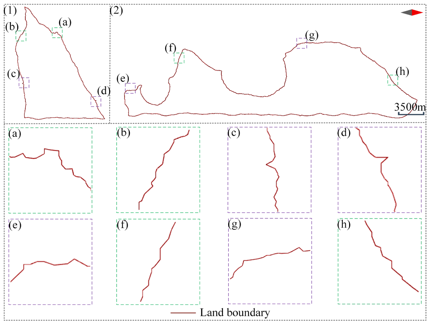
An alpha-shape algorithm was employed to calculate the boundary of the projected land point clouds. Based on the terrain undulation, α was set to 1.3 m, which effectively preserves local concave features along the boundary while suppressing small-scale noise. The boundary was found to contain numerous sharp burrs (Figure 5c–e,g) and sawtooth-like fluctuations (Figure 5a,b,f,h). Overall, the boundary exhibited severe angularization and was dominated by piecewise linear segments.
Figure 5.
Original land boundary (1,2) with magnified views of key segments in (a–h).
3.4. Stage 3: Two-Stage Smoothing of the Land Boundary
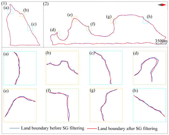
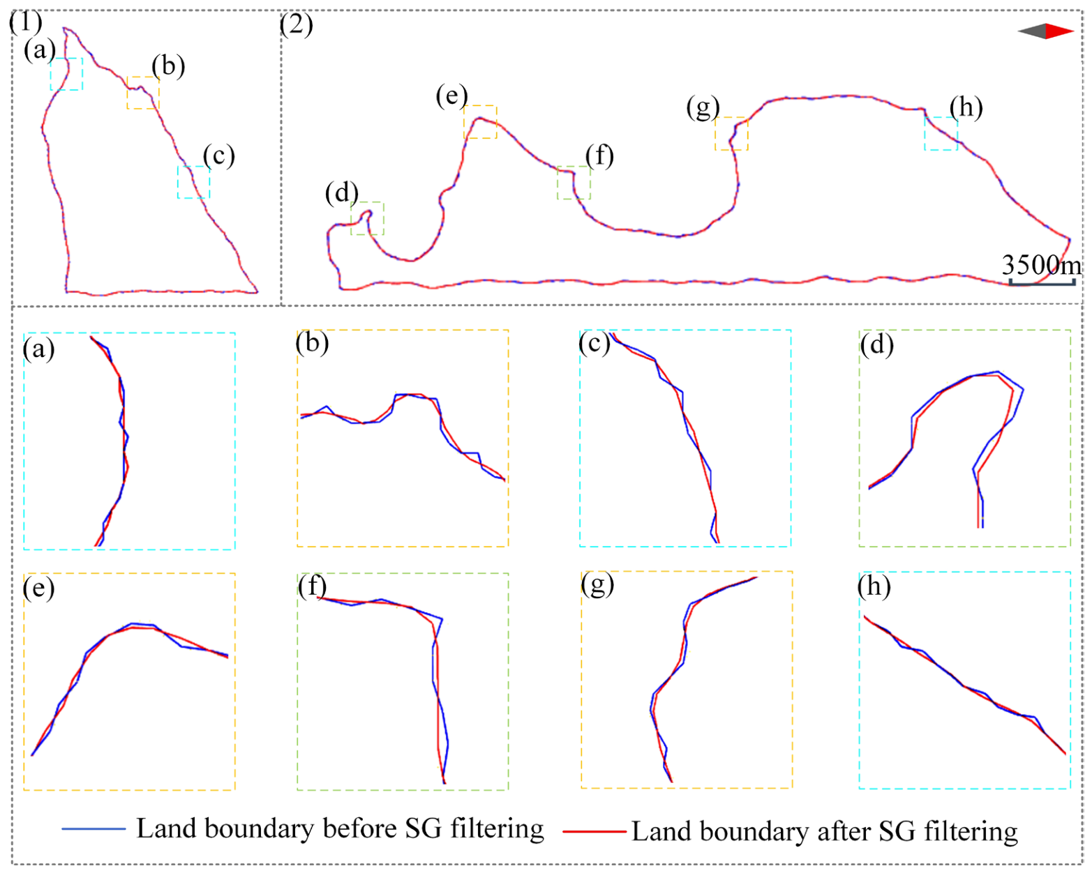
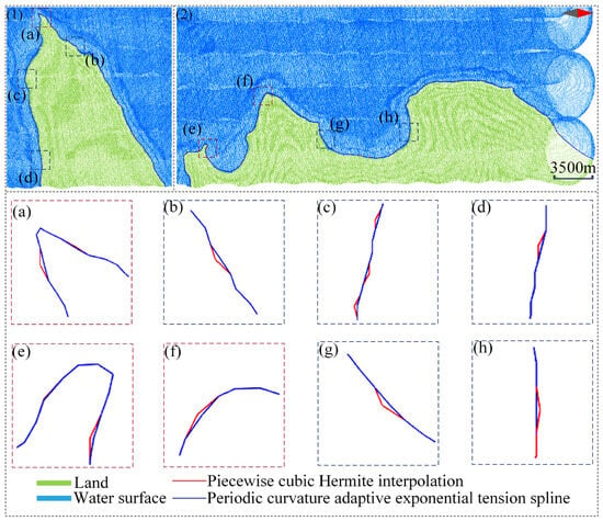
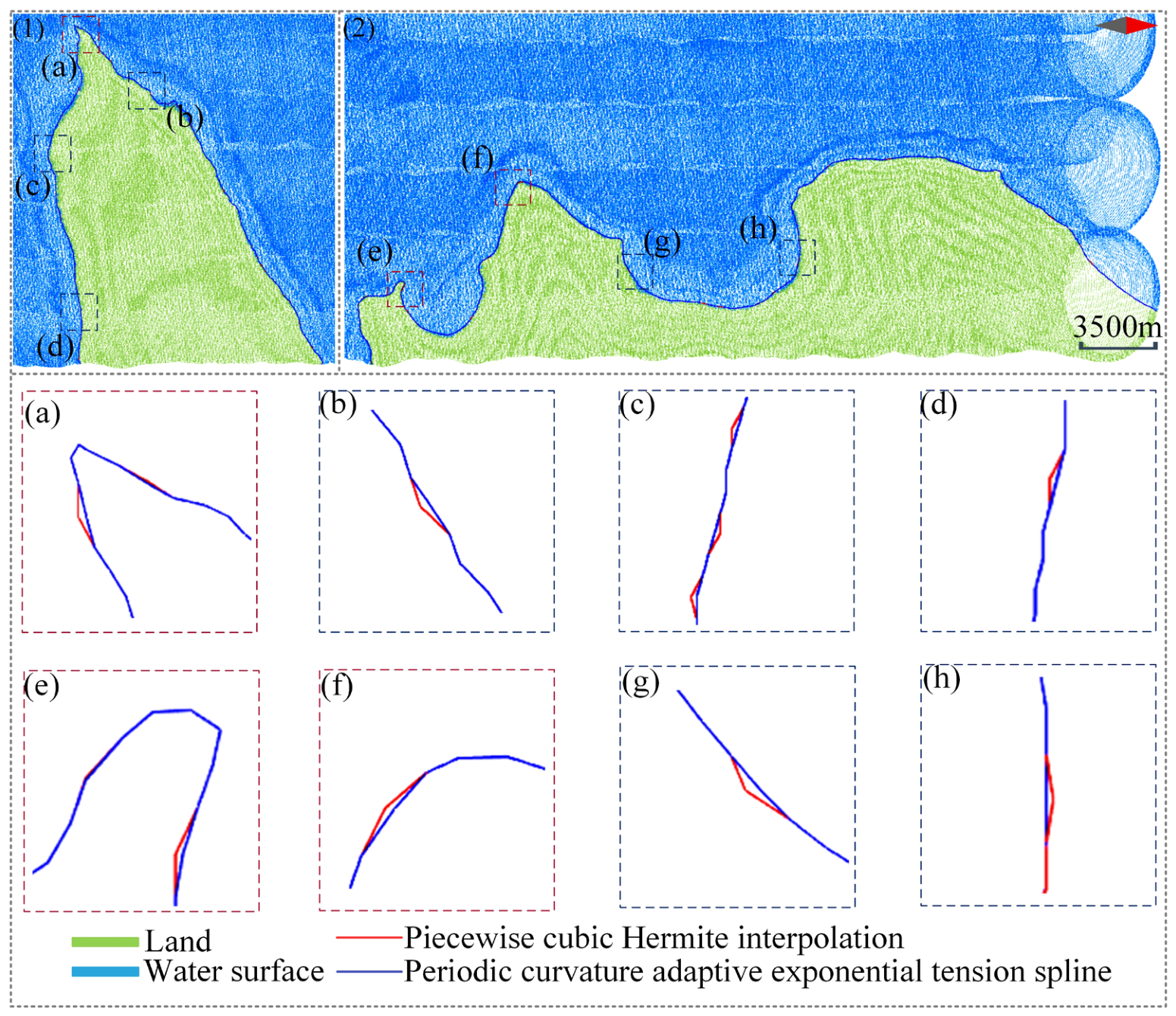
First, a periodic curvature adaptive exponential tension spline was used to reconstruct the discrete land boundary extracted by the alpha-shape. The tension parameters were set to , , and k = 5.50. The spline tension was adaptively adjusted according to the local curvature, maintaining a basic tension in sections with low curvature to ensure overall smoothness. When the local curvature exceeds a set threshold, the tension increases with the curvature, suppressing potential local overshoot and oscillations in high-curvature regions while preserving the main boundary morphology. The curve obtained after adaptive exponential tension spline interpolation is shown in Figure 6 as the land boundary before SG filtering. This curve accurately represents the contour of the land boundary but still exhibits unsmooth transitions at specific inflection points and concave–convex sections.
Figure 6.
Original land boundary before and after SG filtering (1,2), with (a–h) showing magnified views of specific segments.
The second step in this stage was SG filtering, for which equidistant curve points generated by the interpolation curve were used as the input. The window size of SG filtering was set to 11, the polynomial order was 5, and the fitted value at the center of the window was taken as the output of the filtering result at that point. Figure 6 shows the land boundary curves before and after SG filtering. By comparing several representative boundary details, including concave and convex features (Figure 6b,e,g), sharp-turn regions (Figure 6d,f), and gentle-transition regions (Figure 6a,c,h), SG filtering was found to effectively suppress the residual high-frequency micro-oscillations in the spline curve. Sharp corners were transformed into continuous curvature variations and abrupt directional changes transitioned to gently curved segments, thereby further enhancing overall smoothness. This demonstrates that SG filtering not only preserves the geometric fidelity of the original discrete data through interpolation but also suppresses irregular fluctuations through filtering, achieving a balance between preserving the boundary features and smoothness.
3.5. Stage 4: Land–Water Boundary Extraction
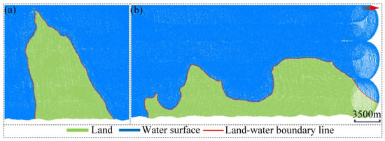
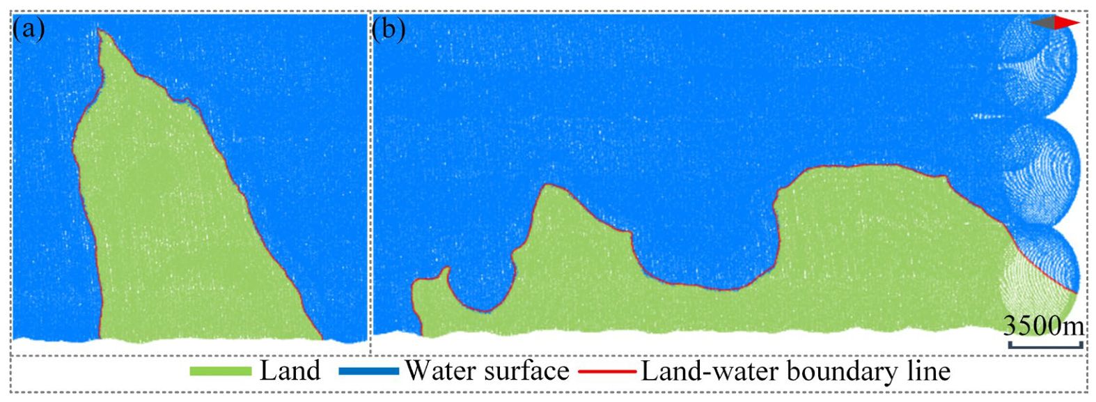
Based on the topographic features of the experimental area, the threshold for determining “near-water-surface” was set to 1 m. After secondary smoothing, the land boundary curve was filtered according to the threshold, and parts that were not adjacent to the water area were filtered out. The results are shown in Figure 7a,b.
Figure 7.
Semi-automatic land–water boundary extraction results: Two land point cloud blocks forming the study area: (a) block 1; (b) block 2. The red curves indicate the land–water boundaries extracted using the proposed method.
4. Results
Due to the complex terrain within the study area, limited accessibility, and safety concerns for the field personnel, conducting in situ measurements using RTK was extremely challenging. Therefore, to verify the accuracy of the method, a set of land–water boundary points was manually extracted from the point cloud. After curve fitting, the manually extracted land–water boundary was obtained and used as a reference for accuracy comparison, and qualitative and quantitative analyses were performed.
4.1. Qualitative Analysis
A comparative evaluation of the proposed two-stage smoothing combination algorithm and the traditional piecewise cubic Hermite interpolation was conducted, followed by SG filtering for land–water boundary extraction; the results are shown in Figure 8. The piecewise cubic Hermite interpolation method is prone to producing sharp corners, burrs, or oscillations in areas with significant curvature changes (Figure 8a,e,f) and areas with gentle morphological changes (Figure 8b–d,g,h). By contrast, the proposed two-stage smoothing combination algorithm maintained a more natural and smooth geometric shape in the same area, suppressed oscillations, and retained details, exhibiting superior local geometric preservation and smoothness.
Figure 8.
Comparison of land–water boundaries under different extraction strategies (1,2), with (a–h) showing magnified views of specific segments.
4.2. Quantitative Analysis
To minimize computational cost while ensuring statistical representativeness, 100 sample points were randomly selected from the manually delineated land–water boundary, and their planar distances to the semi-automatically extracted boundary were calculated. Based on this, the indicators were calculated to evaluate the extraction accuracy quantitatively [33]. The calculation methods are listed in Table 2.
Table 2.
Formulas for calculating accuracy evaluation indicators.
To further strengthen the comparative analysis, a second comparison method combining a uniform periodic B-spline curve with SG filtering was introduced in addition to the piecewise cubic Hermite interpolation followed by SG filtering used in the qualitative analysis. Table 3 presents a quantitative comparison of the extraction errors for the three methods, demonstrating that the proposed two-stage smoothing algorithm achieves higher land–water boundary extraction accuracy.
Table 3.
Calculation errors for different methods.
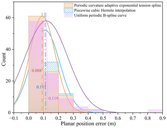
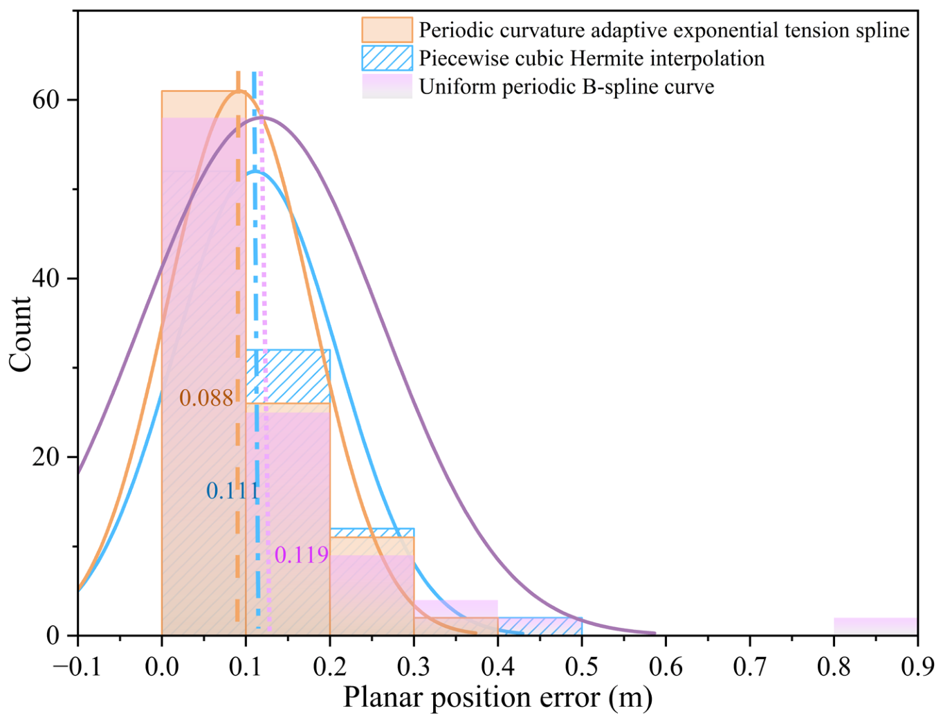
The error distributions of the three interpolation methods are shown in Figure 9. All three follow an approximately normal distribution; however, their error distribution characteristics exhibit notable differences. Based on a statistical analysis of the error intervals, the proposed algorithm shows a high concentration of points in small error ranges and a rapid decline in large error ranges. In contrast, the other two methods exhibit more dispersed error distributions with higher frequencies at large error intervals. In comparison, the mean absolute error of this two-stage smoothing combination algorithm was reduced, with the error mainly concentrated in the range of 0.0–0.2 m. There were fewer local deviation points, and the standard deviation was smaller, indicating that it had a lower dispersion and higher overall stability.
Figure 9.
Distribution of interpolation error intervals.
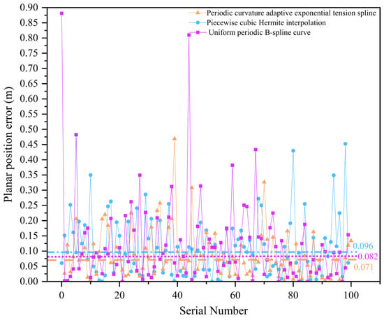
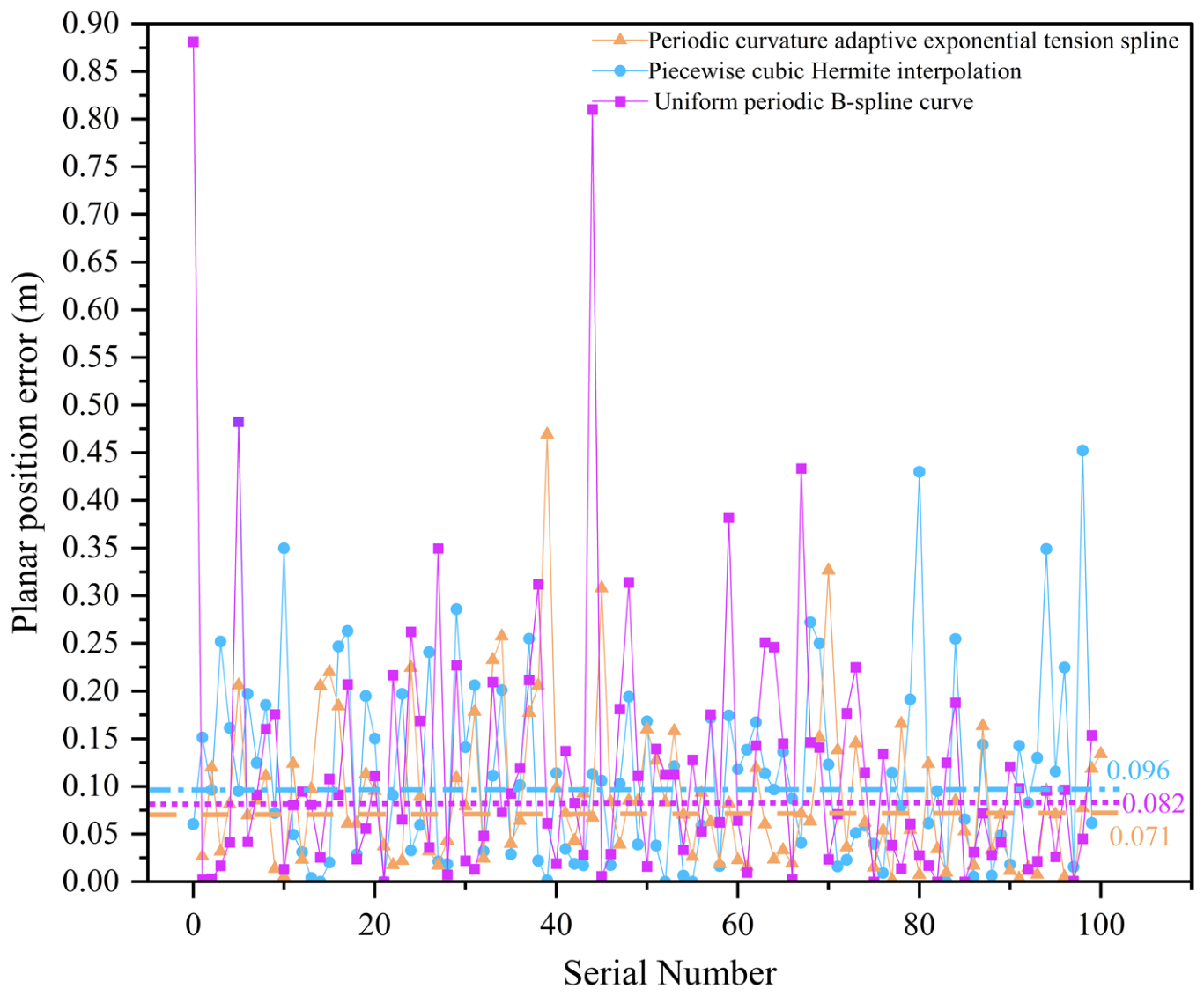
The discrete error distribution in Figure 10 shows that the land–water boundary extracted by the proposed two-stage smoothing combination algorithm has an error of approximately 0.071 m at most locations and exhibits narrow fluctuations. In contrast, the other two methods exhibit not only a larger overall fluctuation range but also higher error values that deviate substantially from the central tendency in certain regions. These findings indicate that the land–water boundary extracted using the two-stage smoothing combination algorithm is less susceptible to noise in areas with drastic local geometric changes and maintains better shape preservation and robustness.
Figure 10.
Discrete distribution of interpolation errors.
4.3. Accuracy Validation in Additional Areas
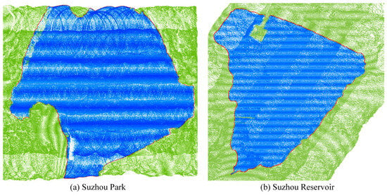
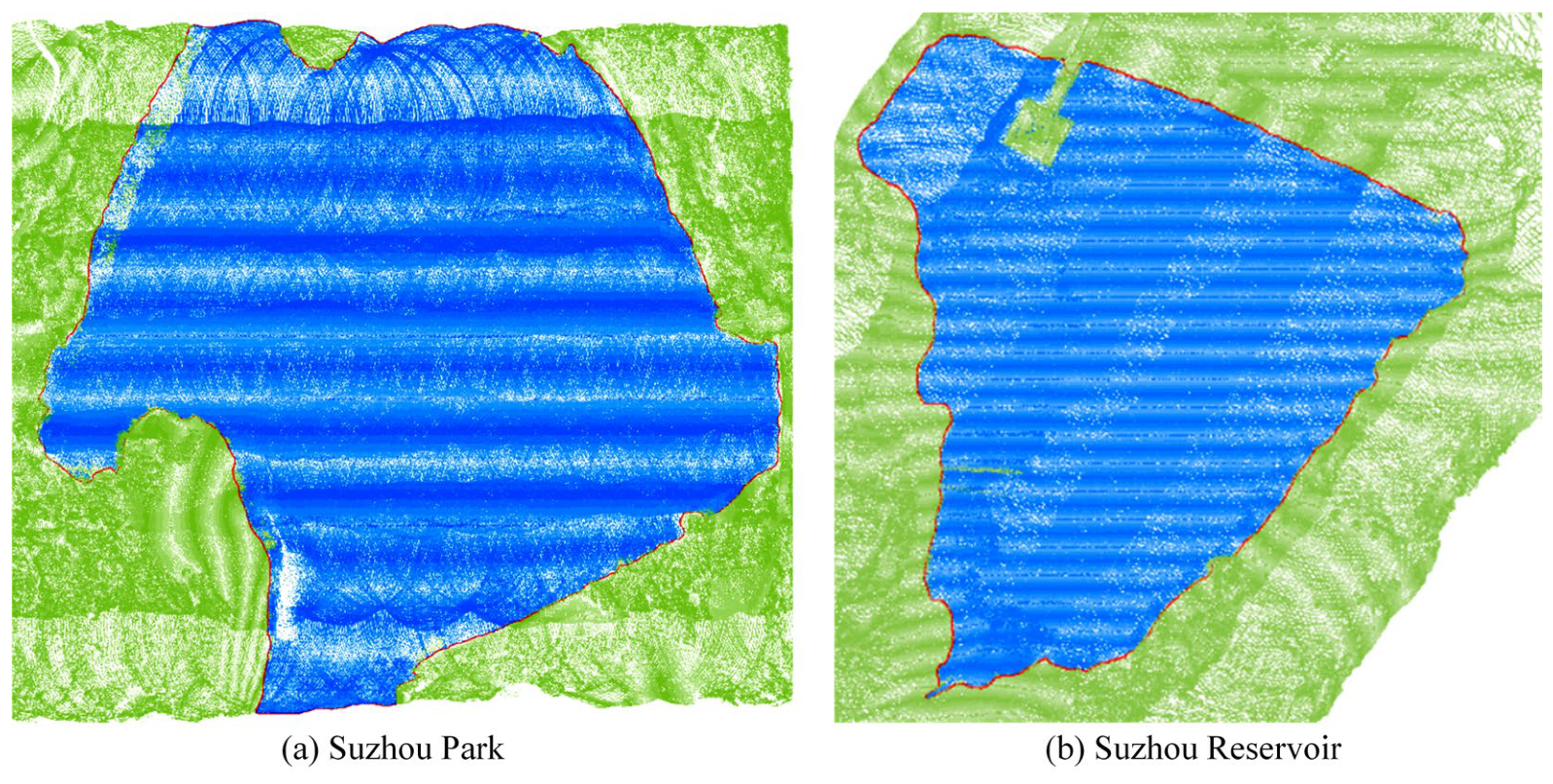
To further evaluate the accuracy of the proposed method, two additional experimental sites, an inland lake and a reservoir, were selected for validation. RTK measurements were conducted to obtain land–water boundary points as reference data. Within the accessible areas, 41 and 49 reference points were acquired at Suzhou Park (as shown in Figure 11a) and Suzhou Reservoir (as shown in Figure 11b), respectively. The findings are detailed in Figure 11 and Table 4.
Figure 11.
(a) Suzhou Park; (b) Suzhou Reservoir. The red curves represent the boundaries extracted for the study areas.
Table 4.
Measured errors at Suzhou Park and Suzhou Reservoir.
According to the results, the proposed method also achieved high accuracy at two other test sites, further verifying the robustness and reliability of the method.
4.4. Processing Efficiency and Comparison with Manual Extraction
The processing times of the main stages of the proposed boundary-extraction procedure were recorded and compared with that of manual boundary extraction (Table 5).
Table 5.
Processing time comparison between manual boundary extraction and the proposed boundary-extraction procedure.
The time for all reports is calculated from after the point cloud denoising is completed and the resulting data is generated. The program takes only 16.25 s to execute, compared to approximately 4.5 h for manual extraction of more than 1000 boundary points. This demonstrates that the proposed method significantly reduces the processing time and workload of manual boundary extraction.
5. Discussion
5.1. Parameter Sensitivity Analysis
5.1.1. Parameters of the Alpha-Shape Algorithm
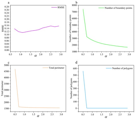
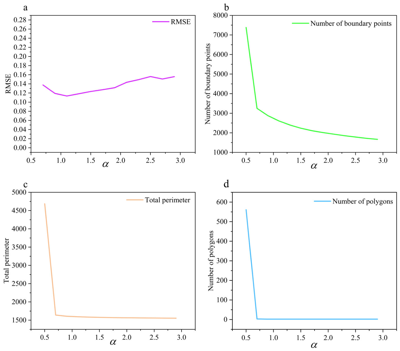
Parameter selection is critical to the accuracy of boundary extraction and requires quantitative justification. To this end, the present study conducted a series of experiments involving a systematic sensitivity analysis of the parameter α within the range of 0.5 to 2.9, evaluating four key metrics—total boundary perimeter, number of boundary points, number of polygons, and random sampling-based RMSE. As shown in Figure 12, the value of α has a significant impact on both the accuracy of shoreline extraction and the resulting boundary morphology.
Figure 12.
Sensitivity of boundary extraction results to the Alpha-Shape parameter α: (a) RMSE; (b) number of boundary points; (c) total perimeter; (d) number of polygons.
When α < 0.9, the alpha shape is highly sensitive to minute gaps and noise in the discrete point cloud, capturing a large number of local depressions. As shown in Figure 12b–d, the total boundary length, the number of boundary points, and the number of polygons all show abnormal growth. When α ≥ 0.9, the topological structure of the boundary tends to stabilize, the number of polygons stabilizes at the actual value of 2, and the total length stabilizes at approximately 1500 m. As shown in Figure 12a, when α is between 0.9 and 1.5, the RMSE remains at a low value. When α continues to increase, small-scale local depressions are ignored, leading to the loss of shoreline details. Considering both positional accuracy and boundary morphology characteristics, this paper sets α = 1.3, which is beneficial for subsequent boundary smoothing and detail representation.
5.1.2. Smoothing Parameters
- Parameters of the periodic curvature adaptive exponential tension spline
To evaluate the impact of the key parameters in periodic curvature adaptive exponential tension spline interpolation on the boundary fitting results, we conducted a sensitivity analysis on the base tension , curvature threshold , and enhancement coefficient k. Using RMSE as the accuracy evaluation metric, the experimental results are illustrated in Table 6.
Table 6.
Sensitivity analysis of the parameters of the periodic curvature adaptive exponential tension spline.
As shown in Table 6, within a reasonable range, the differences in results under different parameter combinations are small, and the relative changes in RMSE do not exceed 0.5%. This indicates that the proposed method has low sensitivity to changes in tension parameters and good parameter stability. When processing datasets with different terrains, there is no need to repeatedly adjust the parameters. Considering the overall positional accuracy, local detail representation, and the avoidance of excessive smoothing of local geometric features due to excessive tension, the final values used are , , and k = 5.50.
- 2.
- Parameters of the SG filter
To evaluate the influence of SG filtering parameters on the boundary extraction results during the secondary smoothing process, we conducted a parameter sensitivity analysis. This involved a combinatorial test of the window size, 2m + 1 (9, 11, and 13), and the polynomial order, n (3, 5, and 7). Using the RMSE, MAE, and standard deviation as evaluation metrics, the corresponding results are presented in Table 7.
Table 7.
Error analysis under different parameter combinations.
When n = 3, some parameter combinations yield relatively low error metrics; however, the stronger smoothing effect tends to oversmooth bends and concave–convex features in high-curvature shoreline regions, resulting in insufficient preservation of local geometric details. When n = 7, higher orders can retain more local variations, but the suppression of high-frequency fluctuations is relatively limited. Therefore, considering the overall positional accuracy, when 2m + 1 = 11 and n = 5, the smoothed boundary can effectively suppress local jaggedness while better preserving the actual morphological characteristics of the shoreline.
5.2. Comparative Analysis with Other Shoreline Extraction Methods
Existing studies indicate that shoreline extraction methods based on optical imagery typically rely on spectral differences between land and water (e.g., water indices, threshold segmentation); their performance is often affected by factors such as lighting conditions, cloud cover, shadows, water turbidity, and surface reflections [12,13]. SAR-based methods are susceptible to speckle noise, vegetation cover, wet shoreline zones, and complex surface scattering, which can reduce shoreline localization accuracy, particularly in areas with complex land-water interfaces [17]. Compared to optical imagery, UAV-ALB acquires spatial information via active laser ranging, thereby exhibiting lower dependence on lighting conditions and greater immunity to interference from cloud cover and shadows. Regarding boundary extraction, UAV-ALB offers advantages in mobility and resolution over image-based methods, providing a novel technical approach for the detailed representation of shorelines. Furthermore, UAV-ALB enables the simultaneous extraction of land-water boundaries and underwater topographic data, offering robust support for applications such as reservoir capacity estimation and 3D hydrological analysis.
To further evaluate the boundary extraction results, the completeness and accuracy metrics proposed by Xu et al. [18] were adopted for comparison. A segmentation threshold of 0.5 m was set, and the extracted shoreline was evaluated against a reference shoreline. The resulting completeness and accuracy rates were 99.50% and 99.67%, respectively, whereas the rates reported by Xu et al. were 92.5% and 90.7%. The results demonstrate a high degree of consistency between the extracted boundaries and the manual reference lines, further validating the performance of the proposed method.
6. Conclusions
In this study, a land–water boundary extraction method based on UAV-borne bathymetric LiDAR point clouds was proposed, providing an effective technical pathway for acquiring shoreline data with high accuracy, strong timeliness, and rich geometric details. By constructing a water surface equation as a reference plane and projecting land point clouds onto this plane, the impact of terrain undulations on the boundary identification was effectively reduced. Then, an alpha-shape algorithm was used to calculate the boundary of the projected land point clouds to achieve fast and accurate boundary extraction. Finally, a combined algorithm of periodic curvature adaptive exponential tension spline interpolation and SG filtering was used to perform two-stage smoothing of the land boundary. The core advantage of the proposed method lies in its ability to dynamically adjust the smoothness according to the boundary curvature, effectively suppressing high-frequency noise and local oscillations. The proposed method outperformed both the traditional piecewise cubic Hermite interpolation method and the combined uniform periodic B-spline curve with SG filtering in terms of extraction accuracy and boundary smoothness. The novel technical solution proposed in this study provides strong support for the efficient extraction of land–water boundaries and the accurate characterization of local shoreline details in inland reservoir and lake environments.
Author Contributions
Conceptualization, Jiayong Yu and Xiaoxue Du; methodology, Jiayong Yu and Xiaoxue Du; software, Jiayong Yu and Jizhe Li; formal analysis, Xiaoxue Du and Jizhe Li; data curation, Maolun Zhou and Deliang Lv; writing—original draft, Jiayong Yu and Xiaoxue Du; writing—review and editing, Maolun Zhou, Jizhe Li, Jing Zhang and Peng Lin. All authors have read and agreed to the published version of the manuscript.
Funding
This study was funded by the National Natural Science Foundation of China (Grant No. 42106180, 42604066), the Major Project of Natural Science Research of Anhui Province (HYB20250132, 2022AH050259), and the Shanghai Science and Technology Plan Project (Grant No. 24xtcx00100).
Data Availability Statement
The data that support the findings of this study are available from the corresponding author, J.L., upon reasonable request.
Conflicts of Interest
Author Maolun Zhou was employed by the company Qingdao Huanhai Offshore Engineering Survey Institute Co., Ltd. The remaining authors declare that the research was conducted in the absence of any commercial or financial relationships that could be construed as a potential conflict of interest.
Abbreviations
The following abbreviations are used in this manuscript:
| UAV | Unmanned aerial vehicle |
| LiDAR | Light Detection and Ranging |
| SG | Savitzky–Golay |
| RMSE | Root mean square error |
| RTK | Real-Time Kinematic |
| ALS | Airborne Laser Scanning |
| ALB | Airborne LiDAR Bathymetry |
| SAR | Synthetic Aperture Radar |
| NDWI | Normalized Difference Water Index |
| MNDWI | Modified Normalized Difference Water Index |
| UAV-ALB | UAV-borne LiDAR bathymetry |
References
- Nevermann, H.; AghaKouchak, A.; Shokri, N. Sea level rise implications on future inland migration of coastal wetlands. Glob. Ecol. Conserv. 2023, 43, e02421. [Google Scholar] [CrossRef] [Scilit]
- San, B.T.; Ulusar, U.D. An approach for prediction of shoreline with spatial uncertainty mapping (SLiP-SUM). Int. J. Appl. Earth Obs. Geoinf. 2018, 73, 546–554. [Google Scholar] [CrossRef] [Scilit]
- Kummu, M.; De Moel, H.; Salvucci, G.; Viviroli, D.; Ward, P.J.; Varis, O. Over the hills and further away from coast: Global geospatial patterns of human and environment over the 20th–21st centuries. Environ. Res. Lett. 2016, 11, 034010. [Google Scholar] [CrossRef] [Scilit]
- Xie, W.; He, Q.; Zhang, K.; Guo, L.; Wang, X.; Shen, J. Impacts of human modifications and natural variations on short-term morphological changes in estuarine tidal flats. Estuaries Coasts 2018, 41, 1253–1267. [Google Scholar] [CrossRef] [Scilit]
- Zhang, Y.; Hou, X. Characteristics of coastline changes on southeast Asia Islands from 2000 to 2015. Remote Sens. 2020, 12, 519. [Google Scholar] [CrossRef] [Scilit]
- Lawrence, P.J.; Evans, A.J.; Jackson-Bué, T.; Brooks, P.R.; Crowe, T.P.; Dozier, A.E.; Jenkins, S.R.; Moore, P.J.; Williams, G.J.; Davies, A.J. Artificial shorelines lack natural structural complexity across scales. Proc. R. Soc. B 2021, 288, 20210329. [Google Scholar] [CrossRef] [Scilit] [PubMed]
- López-Ramade, E.; Mulligan, R.P.; Medellín, G.; Torres-Freyermuth, A. Modelling beach morphological responses near coastal structures under oblique waves driven by sea-breezes. Coast. Eng. 2023, 182, 104290. [Google Scholar] [CrossRef] [Scilit]
- Paravolidakis, V.; Ragia, L.; Moirogiorgou, K.; Zervakis, M.E. Automatic coastline extraction using edge detection and optimization procedures. Geosciences 2018, 8, 407. [Google Scholar] [CrossRef] [Scilit]
- Yu, T.; Xu, S.; Tao, B.; Shao, W. Coastline detection using optical and synthetic aperture radar images. Adv. Space Res. 2022, 70, 70–84. [Google Scholar] [CrossRef] [Scilit]
- Ghosh, M.K.; Kumar, L.; Roy, C. Monitoring the coastline change of Hatiya Island in Bangladesh using remote sensing techniques. ISPRS J. Photogramm. Remote Sens. 2015, 101, 137–144. [Google Scholar] [CrossRef] [Scilit]
- Wang, J.; Wang, L.; Feng, S.; Peng, B.; Huang, L.; Fatholahi, S.N.; Tang, L.; Li, J. An overview of shoreline mapping by using airborne LiDAR. Remote Sens. 2023, 15, 253. [Google Scholar] [CrossRef] [Scilit]
- Pardo-Pascual, J.; Sánchez-García, E.; Almonacid-Caballer, J.; Palomar-Vázquez, J.; Priego de los Santos, E.; Fernández-Sarría, A.; Balaguer-Beser, Á. Assessing the Accuracy of Automatically Extracted Shorelines on Microtidal Beaches from Landsat 7, Landsat 8 and Sentinel-2 Imagery. Remote Sens. 2018, 10, 326. [Google Scholar] [CrossRef] [Scilit]
- Choung, Y.-J.; Jo, M.-H. Comparison between a Machine-Learning-Based Method and a Water-Index-Based Method for Shoreline Mapping Using a High-Resolution Satellite Image Acquired in Hwado Island, South Korea. J. Sens. 2017, 2017, 8245204. [Google Scholar] [CrossRef] [Scilit]
- Ferrentino, E.; Nunziata, F.; Migliaccio, M. Full-polarimetric SAR measurements for coastline extraction and coastal area classification. Int. J. Remote Sens. 2017, 38, 7405–7421. [Google Scholar] [CrossRef] [Scilit]
- Nunziata, F.; Buono, A.; Migliaccio, M.; Benassai, G. Dual-polarimetric C-and X-band SAR data for coastline extraction. IEEE J. Sel. Top. Appl. Earth Obs. Remote Sens. 2016, 9, 4921–4928. [Google Scholar] [CrossRef] [Scilit]
- Schmitt, M.; Baier, G.; Zhu, X.X. Potential of nonlocally filtered pursuit monostatic TanDEM-X data for coastline detection. ISPRS J. Photogramm. Remote Sens. 2019, 148, 130–141. [Google Scholar] [CrossRef] [Scilit]
- Wei, X.; Zheng, W.; Xi, C.; Shang, S. Shoreline extraction in SAR image based on advanced geometric active contour model. Remote Sens. 2021, 13, 642. [Google Scholar] [CrossRef] [Scilit]
- Xu, S.; Ye, N.; Xu, S. A new method for shoreline extraction from airborne LiDAR point clouds. Remote Sens. Lett. 2019, 10, 496–505. [Google Scholar] [CrossRef] [Scilit]
- Li, W.; Liu, L.; Zhu, W.; Li, J.; Liu, T. Shoreline_veget—A new shoreline extraction method for vegetation seas, with high robustness, accuracy and scalability. Front. Mar. Sci. 2025, 12, 1491085. [Google Scholar] [CrossRef] [Scilit]
- Sathish Kumar, M. Extraction of Surface Water Extent: Automated Thresholding Approaches. Environ. Sci. Proc. 2023, 29, 31. [Google Scholar] [CrossRef] [Scilit]
- Cao, H.; Tian, Y.; Liu, Y.; Wang, R. Water body extraction from high spatial resolution remote sensing images based on enhanced U-Net and multi-scale information fusion. Sci. Rep. 2024, 14, 16132. [Google Scholar] [CrossRef] [Scilit] [PubMed]
- Sun, Q.; Li, J. A method for extracting small water bodies based on DEM and remote sensing images. Sci. Rep. 2024, 14, 760. [Google Scholar] [CrossRef] [Scilit] [PubMed]
- Wang, D.; Xing, S.; He, Y.; Yu, J.; Xu, Q.; Li, P. Evaluation of a new lightweight UAV-borne topo-bathymetric LiDAR for shallow water bathymetry and object detection. Sensors 2022, 22, 1379. [Google Scholar] [CrossRef] [Scilit] [PubMed]
- Guo, Y.; Xu, W.; Liu, Y.; Yang, F.; Ji, X. Seafloor Point Refinement for Airborne LiDAR Bathymetry Based on Neighborhood Adaptive Moving Least Squares. IEEE J. Sel. Top. Appl. Earth Obs. Remote Sens. 2025, 19, 295–308. [Google Scholar] [CrossRef] [Scilit]
- He, Y.; Tao, B.; Yu, J.; Xu, G.; Huang, Y. Development of airborne LiDAR bathymetric technology and application. Chin. J. Lasers 2024, 51, 1101016. [Google Scholar] [CrossRef]
- Simon, N.; Piqué, A.; Snyder, D.; Ikuma, K.; Majumdar, A.; Hultmark, M. Fast-response hot-wire flow sensors for wind and gust estimation on UAVs. Meas. Sci. Technol. 2023, 34, 025109. [Google Scholar] [CrossRef] [Scilit]
- Mandlburger, G.; Pfennigbauer, M.; Schwarz, R.; Flöry, S.; Nussbaumer, L. Concept and Performance Evaluation of a Novel UAV-Borne Topo-Bathymetric LiDAR Sensor. Remote Sens. 2020, 12, 986. [Google Scholar] [CrossRef] [Scilit]
- Grayson, B.; Penna, N.T.; Mills, J.P.; Grant, D.S. GPS precise point positioning for UAV photogrammetry. Photogramm. Rec. 2018, 33, 427–447. [Google Scholar] [CrossRef] [Scilit]
- Specht, M.; Specht, O. Accuracy Assessment of Shoreline Extraction Using MLS Data from a USV and UAV Orthophoto on a Complex Inland Lake. Remote Sens. 2025, 17, 3940. [Google Scholar] [CrossRef] [Scilit]
- Vélez-Nicolás, M.; García-López, S.; Barbero, L.; Ruiz-Ortiz, V.; Sánchez-Bellón, Á. Applications of Unmanned Aerial Systems (UASs) in Hydrology: A Review. Remote Sens. 2021, 13, 1359. [Google Scholar] [CrossRef] [Scilit]
- Hu, S.; He, Y.; Tao, B.; Yu, J.; Chen, W. Classification of sea and land waveforms based on deep learning for airborne laser bathymetry. Infrared Laser Eng. 2019, 48, 1113004. [Google Scholar] [CrossRef] [Scilit]
- Cao, R.; Sheng, Y.; Dong, A.; Liu, H. Design of a Savitzky-Golay filter-based vEMG-FES system. IEEE Trans. Neural Syst. Rehabil. Eng. 2025, 33, 610–619. [Google Scholar] [CrossRef] [Scilit] [PubMed]
- Leach, R.; Haitjema, H.; Su, R.; Thompson, A. Metrological characteristics for the calibration of surface topography measuring instruments: A review. Meas. Sci. Technol. 2021, 32, 032001. [Google Scholar] [CrossRef] [Scilit]

Disclaimer/Publisher’s Note: The statements, opinions and data contained in all publications are solely those of the individual author(s) and contributor(s) and not of MDPI and/or the editor(s). MDPI and/or the editor(s) disclaim responsibility for any injury to people or property resulting from any ideas, methods, instructions or products referred to in the content. |
© 2026 by the authors. Published by MDPI on behalf of the International Society for Photogrammetry and Remote Sensing. Licensee MDPI, Basel, Switzerland. This article is an open access article distributed under the terms and conditions of the Creative Commons Attribution (CC BY) license.