GIS-Based Multi-Stop UAV Routing for Emergency Medical Delivery in Khartoum, Sudan: Priority-Aware Optimisation and Deep Reinforcement Learning

Abstract

Routing a medical-delivery UAV to multiple hospitals must jointly account for distance, flight time, payload, and clinical priority. We present a reproducible GIS-based framework for multi-stop UAV emergency medical routing in Khartoum State, Sudan, using a common obstacle-aware 3-D leg model with grid-based A* routing around no-fly zones and payload-dependent climb, cruise, and descent. We show that a linear priority term in a composite tour cost is order-invariant and cannot distinguish visiting sequences. We therefore use a priority-weighted completion-time objective with hard deadlines for Critical hospitals, with criterion weights derived from health professionals using the Analytic Hierarchy Process. On a 14-hospital network, exact Held–Karp and label-setting dynamic programming provide proven optima for benchmarking classical, metaheuristic, and Advantage Actor–Critic sequencing methods (A2C-SP). The revised objective reduces optimal priority-weighted completion time by 14% with only a 0.2% increase in distance. A2C-SP is 14.7% above the optimum across 47 unseen instances while generating routes in approximately 2 ms. Without retraining, it also plans capacity- and range-feasible multi-sortie missions on a 59-hospital city network, achieving a priority-weighted completion time of 110 min versus 137 min for the published toolbox route. At city scale, a single UAV cannot serve more than 5 of 16 Critical hospitals within 15 min, highlighting fleet sizing as a key constraint for meeting such deadlines.

1. Introduction

Delivering life-critical medical supplies—blood products, cardiac medications, emergency anaesthetics—to the right hospital at the right time is one of the most consequential logistics problems in emergency healthcare. In Khartoum State, Sudan, the problem is compounded by chronic road congestion across a metropolitan area of more than seven million residents, deteriorating road infrastructure, and a geography split by the confluence of the Blue and White Nile rivers. The bridges that connect the conurbation’s three districts become acute bottlenecks at peak hours, and at least two of these bridges have sustained conflict-related damage, further constraining an already congested cross-river network amid the wider humanitarian disruption documented across the country [1].

UAV-based delivery has shown operational value under similar conditions elsewhere: a retrospective evaluation of Rwanda’s national drone network found blood-product delivery by UAV took a mean of 49.6 min against a median of 120 to 139 min by road, alongside a 67% reduction in blood-unit wastage [2], a gain concentrated exactly where roads are slowest. Khartoum’s road-dependent, congestion-prone supply chain suggests UAV routing is a tractable near-term intervention there too.

Routing a single UAV between two points is well understood: the A* algorithm [3], with evaluation function f(n) = g(n) + h(n), returns the shortest obstacle-aware path whenever its heuristic is admissible. The harder, operationally more consequential problem is deciding the visiting order across many hospitals before returning to the dispatch hub, a multi-criteria variant of the Travelling Salesman Problem in which the objective is not pure distance but a weighted combination of distance, flight-plus-service time, payload, and clinical priority.

This study compares six sequencing strategies and a learned policy under a single, shared, explicitly defined objective, rather than allowing each algorithm to optimise a differently formulated objective. All methods are evaluated against proven optima. The comparison includes a one-pass greedy rule, classical constructive heuristics with local-search refinement, simulated annealing, a genetic algorithm, the Google OR-Tools routing solver, and a trained Advantage Actor–Critic sequencing policy, for which we report the deployed policy behaviour rather than its best observed training episode. The research questions are (i) can a composite tour cost with a linear priority term favour Critical hospitals, and if not, which alternative objective can do so; (ii) how far from optimal are the heuristics, metaheuristics, and learned policy on a real obstacle-aware hospital network; and (iii) can a policy trained once generalise to unseen networks, alternative weightings, and multi-sortie missions under payload and range constraints?

This study addresses the following research gap. Previous UAV medical-delivery studies either route a single origin-destination leg or optimise multi-stop tours with a distance- or energy-based cost, and learning-based routing studies are usually evaluated on synthetic Euclidean instances without proven optima. To our knowledge, no study has shown that the linear priority term commonly used in composite tour costs cannot change the optimal visiting order, replaced it with a deadline-constrained, priority-weighted completion-time objective, and measured classical heuristics, metaheuristics, an industrial routing solver (Google OR-Tools) and a learned sequencing policy against proven optima on the same obstacle-aware GIS network of a real city. This study fills that gap for Khartoum: the leg model and the objective are fixed for all methods, so differences in the results can be attributed only to how each method chooses the visiting order, and a policy trained once is tested on unseen networks and on multi-sortie missions.

Key Contributions

In every method evaluated in this study, grid-based A* computes the obstacle-aware geometry of each leg using the same procedure. The methods differ only in how they determine the visiting sequence and, when payload or range constraints require multiple sorties, how they partition the sequence into sorties. The learned policy does not modify the A* leg model. The main contributions are:

• reproducible GIS-to-optimisation pipeline in which a single 3-D leg model and a single objective are shared across all methods. An ArcGIS-independent re-implementation reproduces the ArcGIS PrArcGIS Pro (version 3.4.0; Esri, Redlands, CA, USA) runso runs, with distance and time residuals below ${10}^{-9}$ m and s, respectively, enabling every experiment to be repeated from the exported leg matrices (Supplementary Materials).
• A proof that a linear priority term in a composite tour cost is order-invariant, together with a corrected formulation based on priority-weighted completion time with hard, priority-specific deadlines and explicit priority-violation metrics.
• Proven optimal benchmarks obtained using Held–Karp and label-setting dynamic programming, cross-checked by brute-force enumeration and mixed-integer linear programming (MILP), together with the Google OR-Tools solver. These benchmarks provide optimality gaps for six routing methods on a real, conflict-affected urban hospital network, using criteria weights elicited from health professionals.
• A size-invariant, preference-conditioned Advantage Actor–Critic sequencing policy (A2C-SP) that incorporates payload and range constraints into the MDP. The policy is trained once on random sub-networks and evaluated for generalisation to unseen networks, alternative weightings, and multi-sortie missions, including a multi-seed hyperparameter study.

2. Literature Review

2.1. UAV Medical Delivery in Urban and Resource-Constrained Environments

The evidence base for UAV medical delivery has expanded substantially. Rwanda’s national drone network demonstrated a mean blood-product delivery time of 49.6 min against 120 to 139 min by road, and a 67% reduction in blood-unit wastage [2]. Haidari et al. [4] modelled drone-based vaccine delivery for Gaza Province, Mozambique, finding vaccine availability rose from 94% to 96% while logistics costs fell by roughly 20% relative to conventional multi-tiered land transport. Scott and Scott [5] reviewed drone delivery models for healthcare logistics and proposed network-design models to improve delivery timeliness. Boutilier and Chan [6] modelled drone networks for cardiac-arrest response across the Toronto, Canada area, projecting substantially higher survival rates through faster automated-external-defibrillator delivery. These studies converge on routing-algorithm quality and spatial-data accuracy as the primary performance determinants, which motivates the algorithmic comparison presented here. Khartoum adds constraints largely absent from these prior studies—a multi-bank geography, conflict-adjacent airspace restrictions, and a hospital network spread across three administratively distinct districts—which raise both the difficulty and the stakes of multi-stop routing relative to the single-route scenarios that dominate much of the UAV-delivery literature [7]. In our previous work on the same city [8], five pathfinding algorithms (A*, Dijkstra, breadth-first, depth-first and greedy best-first search) were benchmarked for single-route UAV delivery over 62 hospital routes in Khartoum and compared with road transport, and a multi-criteria urgency score was implemented in ArcGIS Pro toolboxes; the present study builds on that framework and addresses the multi-stop sequencing problem. Beyond routing, practical UAV missions must also cope with external disturbances such as wind gusts, which robust flight controllers are designed to reject [9], and multi-UAV operations require coordination among the vehicles, for which leader-following consensus schemes robust to external disturbances have been proposed [10]. These operational aspects are outside the scope of the present routing study, but they become relevant when the fleet-sizing implications of Section 5.7 are put into practice.

2.2. A* Pathfinding and Multi-Stop Routing

Hart et al. [3] established A* as the canonical admissible-heuristic search algorithm: its evaluation function adds the accumulated path cost to a consistent lower-bound heuristic, and it returns the shortest path whenever the heuristic never overestimates the true cost. Dijkstra’s algorithm [11] is the special case with a zero heuristic; it is complete and optimal but explores more nodes in practice. UAV transport of medical products is recognised as operationally feasible [12,13], which motivates a principled path-finding method such as A* for each leg. For multi-stop routing, however, A* only computes the geometry of individual legs; the visiting order is a separate combinatorial problem whose exhaustive solution grows as O(n!) with the number of hospitals. Exact methods for the TSP, such as the Held–Karp dynamic programme [14] and mixed-integer formulations with Miller–Tucker–Zemlin subtour constraints [15], are computationally feasible for the sortie sizes considered in this study and therefore provide proven optima against which approximate methods can be evaluated. When time windows are imposed, label-setting extensions of dynamic programming provide an exact solution approach [16].

2.3. Metaheuristics for Vehicle Routing and the Travelling Salesman Problem

Where exhaustive search is impractical, metaheuristics can provide approximate solutions at substantially lower computational cost. Genetic algorithms explore the permutation space through selection, crossover, and mutation and are widely used as baselines for multi-stop routing and vehicle-routing problems. Simulated annealing combined with 2-opt local search is likewise well established for the TSP and capacitated vehicle routing problem (CVRP), including recent applications to homogeneous CVRP instances [17]. Google’s OR-Tools routing library [18] provides a widely used optimisation solver for routing applications and serves here as a direct benchmark. In this study, OR-Tools is run directly with time-window constraints representing the Critical deadlines, rather than being replaced by a fallback procedure.

2.4. Deep Reinforcement Learning for Combinatorial Routing

Deep reinforcement learning (DRL) has emerged as an approach to combinatorial routing when exhaustive optimisation becomes computationally demanding. Li et al. [19] applied DRL with dynamic spatio-temporal graphs to urban logistics planning and reported faster and better solutions than a commercial solver and classical heuristics on the tested instances. Two recent systematic reviews highlight both the potential and the reporting challenges of this literature. Liu, Demir, and Jian [20] reviewed 129 DRL studies on vehicle routing and found that most either formulate the problem directly as a Markov decision process or combine reinforcement learning with heuristic methods. Martins, Sousa, and Vieira [21] reviewed 298 studies of DRL for industrial combinatorial optimisation, identifying state representation, action-space design, and reward design as key factors affecting reproducibility, while noting that scalability to larger instances remains an open issue. In response, the present study trains on randomly generated sub-networks and evaluates the policy on unseen networks containing 14 and 59 hospitals.

Taresh, Asgharian Sardroud, and Tajbakhsh [22] applied proximal policy optimisation to a multi-agent truck-and-drone TSP and reported improvements in delivery efficiency and scalability from decentralised policies. This provides evidence for the applicability of policy-gradient methods to drone-related sequencing problems, alongside the REINFORCE/actor–critic family used here [23,24]. Damos et al. [25] proposed a DRL-assisted ant colony optimisation approach in which an agent learns the pheromone-update rule using an AHP-weighted reward combining distance, time, and energy, and reported shorter paths and faster convergence than classical ant colony optimisation and a genetic algorithm in a UAV case study in Sudan. The present study differs in scope: the learned policy directly determines the hospital-visiting sequence and is evaluated against non-learned baselines under a single shared objective.

Attention-based encoder–decoder policies [26,27,28] and pointer-network approaches trained with policy gradients [29] use architectures whose parameters are not tied to a fixed number of nodes, allowing them to be applied to instances of different sizes. We adopt this size-invariant design.

The REINFORCE policy-gradient algorithm [23], together with an actor–critic architecture that separates the policy network (actor) from the value estimator (critic), provides the training foundation used here. The advantage (A_t = G_t − V(s_t)) reduces gradient variance, while entropy regularisation [24] discourages premature convergence to a deterministic policy. A recurring reporting issue in this literature is to present the best sequence observed during training as representative of deployed performance. In this study, performance is instead reported from the deployed policy itself.

2.5. Multi-Criteria Decision Making in Medical Logistics

Integrating clinical urgency into routing distinguishes medical logistics from generic TSP formulations. The Analytic Hierarchy Process (AHP) [30] derives relative weights for competing criteria. In this study, distance, flight-plus-service time, payload, and patient priority are derived from pairwise comparisons. The criteria weights are elicited from a panel of health professionals, and individual judgements are aggregated using the geometric mean [31,32], GIS-based AHP decision frameworks implemented as Python (Python 3.11, Python Software Foundation, Wilmington, DE, USA; 2 CPU cores) models in ArcGIS Pro have also been applied to other urban services in Khartoum State, such as landfill siting and solid-waste collection [33].

However, weighting these criteria within a conventional tour-cost formulation does not by itself ensure that higher-priority hospitals are served earlier. This limitation motivates an objective that explicitly depends on service order and completion time. Scheduling theory provides such formulations through weighted completion-time and time-window objectives [16], while priority-aware reinforcement learning can incorporate task priority into the state and reward design [34].

2.6. Positioning Against the Closest Studies

Table 1 contrasts the present study with closely related work. Drone-routing models incorporating capacity and energy constraints [35,36] have been addressed using exact and heuristic optimisation methods, but without learned sequencing policies or explicit clinical priority. Learning-based routing studies [19,22,26,27] report generalisation across synthetic Euclidean instances, but typically do not benchmark against proven optima on real, obstacle-aware networks. Priority-aware DRL [34] incorporates task priority into the state and reward, a design principle adopted in the present study. Damos et al. [25] integrate DRL into ant-colony optimisation for UAV path planning rather than using a learned policy to determine the multi-hospital visiting sequence.

Table 1. Positioning of this study against the closest related work.

Study	Problem	Priority/Deadlines	Payload/Range	Exact Benchmark	Learned Policy Tested on Unseen Instances	Real GIS Obstacles
Dorling et al. [35]	Multi-trip drone VRP	No	Yes/energy	MILP (small)	-	No
Murray and Chu [36]	Truck-drone TSP	No	Yes/endurance	MILP	-	No
Nazari et al. [26]	CVRP	No	Yes/No	No (heuristics)	Yes (synthetic)	No
Kool et al. [27]	TSP, CVRP, OP	No	Yes/No	Concorde/Gurobi (TSP)	Yes (synthetic)	No
Li et al. [19]	Urban logistics VRP	Time windows	Yes/No	Commercial solver	Yes	Road graph
Taresh et al. [22]	TSP with drones	No	Partly	No	Partly	No
Hao et al. [34]	Priority-aware offloading	Yes	-	No	Yes	-
Damos et al. [25]	UAV path planning	No (AHP reward)	No	No	No	Field case
This study	Multi-stop, multi-sortie medical UAV	Yes: weighted completion + hard deadlines	Yes/Yes	Held–Karp/label DP, MILP, OR-Tools	Yes (unseen 14- and 59-hospital networks)	Yes (Khartoum)

To our knowledge, the combination considered here—proven optimal benchmarks, direct use of the Google OR-Tools solver, hard clinical deadlines, and a size-invariant learned sequencing policy evaluated on a GIS-based obstacle model of a real city—has not been systematically evaluated in prior work. This study therefore positions learned sequencing within a common, reproducible benchmarking framework in which all methods use the same leg model and objective.

3. Methodology

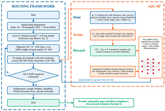
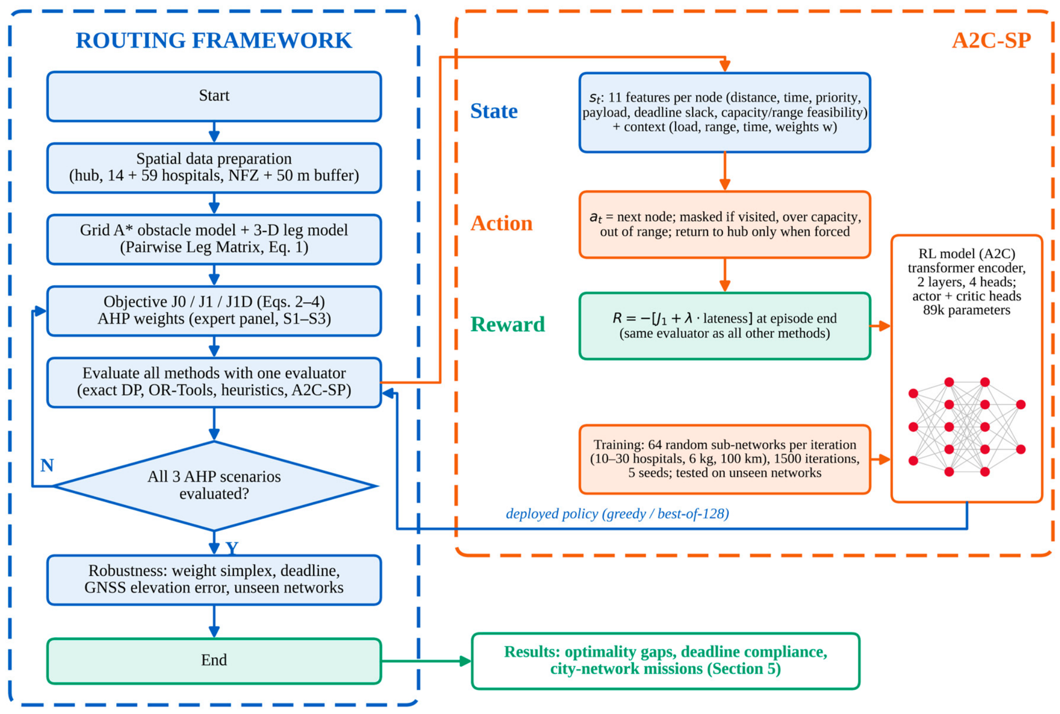
Figure 1 summarises the shared workflow described below: spatial data preparation, obstacle-aware 3-D leg modelling, and a single objective applied consistently across all methods, followed by exact benchmarks, heuristics and solvers, the learned sequencing policy, and the evaluation design used to generate the results presented in Section 5.

Figure 1.  Framework of the study. All methods share the same leg geometry (steps 1-2) and the same evaluator of the objective (step 3); they differ only in how they choose the visiting sequence (step 4).

3.1. UAV Operational Parameters and 3-D Leg Model

The ground elevation $z_i$ (m above mean sea level) of the hub and the 14 hospitals was surveyed in the field using a handheld GNSS receiver (Sokkia GRX2)handheld GNSS receiver (GRX2; Sokkia, Atsugi, Japan) in January 2023. Because vertical error in handheld GNSS measurements is reported to be roughly twice the horizontal error [37], elevation uncertainty is considered in the sensitivity analysis. For the city network, the elevation attribute of the OpenStreetMap layer is a placeholder sequence (291–355) rather than measured values; a flat-terrain assumption is therefore adopted by assigning the surveyed hub elevation to all nodes of that network, and Section 5.6 shows that flat terrain does not change the optimal route.

The UAV (JOUAV CW-25E, a VTOL fixed-wing platform) takes off vertically, climbs to a constant cruise altitude of $h_{cruise}=380$ m AMSL, follows the obstacle-aware horizontal path, descends vertically, and lands at every hospital for a 60 s service time before taking off again. The resulting vertical offsets $h_i=h_{cruise}-z_i$ range from 75 to 105 m in the study area. These offsets are below the commonly used 120 m above-ground operating ceiling for small UAVs. For a leg $i\to j$ flown with payload $q$ on board:

$$d_{ij}=h_i+H_{ij}+h_j, t_{ij}\left(q\right)={\displaystyle \frac{{\tau }_{ij}+h_i/v_{\mathrm{a}\mathrm{s}\mathrm{c}}+h_j/v_{\mathrm{d}\mathrm{e}\mathrm{s}\mathrm{c}}}{\mathrm{m}\mathrm{a}\mathrm{x}\left(0.3,\hspace{0.25em}1-0.01q\right)}}+s_j$$

(1)

where H_ij is the length of the grid-A* path and τ_ij its unloaded horizontal flight time at 19 m/s, including the turn-angle speed penalty of the toolbox; v_asc = 3 m/s and v_desc = 2.5 m/s; and s_j = 60 s at hospitals and 0 at the hub. The multiplier max (0.3, 1 − 0.01q) scales all three speeds, so the flight time for any payload on board follows exactly from the unloaded flight time. Table 2 lists the operational parameters, identical for all methods.

Table 2. UAV operational parameters, identical for all methods (corrected: the cruise altitude is 380 m above mean sea level, not above ground level).

Parameter	Value	Description
Cruise altitude	380 m AMSL	75–105 m above ground in the study area
Horizontal speed (unloaded)	19 m/s	Nominal airspeed before payload adjustment
Ascent/descent speed (unloaded)	3/2.5 m/s	Vertical take-off and landing at every stop
Payload speed multiplier	max (0.3, 1 − 0.01q)	q = payload on board (kg); scales all speeds
Service time per stop	60 s	Landing, hand-over and take-off at each hospital
Obstacle safety margin	50 m	Outward buffer around no-fly-zone polygons
Grid cell size	50 m	Navigation-grid resolution for A*
Max payload capacity Wmax	6 kg	Per sortie; also, normalisation constant
Max flight range per sortie	100 km	Mission feasibility constraint
Spatial reference	EPSG:32636	WGS 84/UTM zone 36N
Drone model	JOUAV CW-25E	VTOL fixed-wing platform

Table 2. UAV operational parameters, identical for all methods (corrected: the cruise altitude is 380 m above mean sea level, not above ground level).

Parameter	Value	Description
Cruise altitude	380 m AMSL	75–105 m above ground in the study area
Horizontal speed (unloaded)	19 m/s	Nominal airspeed before payload adjustment
Ascent/descent speed (unloaded)	3/2.5 m/s	Vertical take-off and landing at every stop
Payload speed multiplier	max (0.3, 1 − 0.01q)	q = payload on board (kg); scales all speeds
Service time per stop	60 s	Landing, hand-over and take-off at each hospital
Obstacle safety margin	50 m	Outward buffer around no-fly-zone polygons
Grid cell size	50 m	Navigation-grid resolution for A*
Max payload capacity Wmax	6 kg	Per sortie; also, normalisation constant
Max flight range per sortie	100 km	Mission feasibility constraint
Spatial reference	EPSG:32636	WGS 84/UTM zone 36N
Drone model	JOUAV CW-25E	VTOL fixed-wing platform

The values follow the UAV platform and the study area. For the JOUAV CW-25E the manufacturer reports a cruising speed of 72 km/h (20 m/s), an endurance of up to 240 min and flight distances of up to 200 km [38]; we use a slightly conservative 19 m/s and a range of 100 km per sortie, half the reported distance, as a reserve for wind, hovering and the return leg. The 6 kg payload capacity and the 60 s service time (landing, hand-over and take-off) are mission assumptions of this study. The cruise altitude of 380 m AMSL keeps the UAV 75–105 m above ground, below the common 120 m ceiling for small UAVs. Because these values affect distance, flight time and feasibility, their sensitivity is tested in Section 5.6 (Table A2).

3.2. Obstacle Model

No-fly-zone polygons representing airport, military, and government areas are buffered outward by a 50 m safety margin and rasterised onto a navigation grid with 50 m cells. For every ordered pair of nodes, A* with the octile heuristic searches the 8-connected grid; diagonal moves are not permitted to cut across blocked corners. The resulting cell path is then shortened using line-of-sight string-pulling, retaining only the turning points required to maintain clearance from blocked cells. The octile heuristic is admissible and consistent for the adopted grid and movement costs; therefore, A* returns the shortest path on the navigation grid. All methods use the same pairwise leg geometry, exported by the toolbox as the Pairwise Leg Matrix. Consequently, differences between methods arise from their sequencing and sortie-partitioning decisions rather than from differences in obstacle-aware leg construction.

3.3. Objective Functions

The published objective, $J_0$, is the composite leg cost used in the previous version of the toolbox. With payload $q$ still on board, the leg cost is

$$c_{ij}\left(q\right)=w_1{\displaystyle \frac{d_{ij}}{D_{\mathrm{m}\mathrm{a}\mathrm{x}}}}+w_2{\displaystyle \frac{t_{ij}\left(q\right)}{T_{\mathrm{m}\mathrm{a}\mathrm{x}}}}+w_3{\displaystyle \frac{q}{W_{\mathrm{m}\mathrm{a}\mathrm{x}}}}-w_4{p}_j$$

(2)

Proposition 1

(order invariance). For any complete tour $\pi$ that serves each hospital $j\in H$ exactly once and returns to the hub ($p_{\mathrm{h}\mathrm{u}\mathrm{b}}=0$), the priority component of $J_0\left(\pi \right)$ equals $-w_4{\sum }_{j\in H}{p}_j$. This value is identical for every complete tour. Therefore, $\arg \min J_0$ is independent of $w_4$ and of the hospital priorities.

This holds because each hospital appears exactly once as a leg destination.

Proposition 1 explains why changing the priority weight in Equation (2) cannot guarantee earlier service of Critical hospitals. For one-step greedy rules, however, the corresponding priority contribution is not constant because the rule evaluates individual candidate destinations; this explains why a greedy rule can select Critical hospitals early.

In the revised objective, $J_1$, let $C_j\left(\pi \right)$ denote the completion time of hospital $j$ along tour $\pi$, measured at landing after completion of the associated service time. Clinical priority is incorporated through the priority-weighted completion time:

$$J_1\left(\pi \right)=\sum _{\left(i,j\right)\in \pi }\left[w_1{\displaystyle \frac{d_{ij}}{D_{\mathrm{m}\mathrm{a}\mathrm{x}}}}+w_2{\displaystyle \frac{t_{ij}\left(q\right)}{T_{\mathrm{m}\mathrm{a}\mathrm{x}}}}+w_3{\displaystyle \frac{q}{W_{\mathrm{m}\mathrm{a}\mathrm{x}}}}\right]+w_4{\displaystyle \frac{\sum _{j\in H}{p}_j\hspace{0.17em}{C}_j\left(\pi \right)}{T_{\mathrm{m}\mathrm{a}\mathrm{x}}\sum _{j\in H}{p}_j}}$$

(3)

The final term is the priority-weighted mean completion time normalised by $T_{\mathrm{m}\mathrm{a}\mathrm{x}}$, and unlike the priority term in $J_0$, it depends on the visiting order. It can be decomposed over successive legs as $w_4{t}_{ij}{P}_{\mathrm{o}\mathrm{p}\mathrm{e}\mathrm{n}}/\left(T_{\mathrm{m}\mathrm{a}\mathrm{x}}{\sum }_j{p}_j\right)$, where $P_{\mathrm{o}\mathrm{p}\mathrm{e}\mathrm{n}}$ denotes the priority mass of hospitals not yet served. This permits incremental evaluation during route construction by all methods.

Hard deadlines can be added to the revised objective, giving the deadline-constrained variant $J_{1D}$, in which each priority class $k$ can be assigned a latest completion time ${\mathsf{\Delta }}_k$. In this study, Critical hospitals are assigned a 15 min deadline. This value is used as a service-target benchmark based on the NHS England Category-1 ambulance response standard of 15 min at the 90th centile [39]. Separately, evidence from prehospital blood transfusion in combat medical evacuation has examined the association between transfusion timing and mortality, including transfusion initiated within 15 min of MEDEVAC rescue [40]. These sources provide contextual benchmarks rather than a UAV-specific regulatory standard.

Because the 15 min value is treated as a service-target benchmark, Section 5.6 reports results over deadlines ranging from 13.0 to 60 min. A Critical hospital that cannot be reached within the deadline even by an empty UAV on a direct flight is considered outside the corresponding hub coverage. In the present network, Soba University Hospital requires 15.2 min under this test and is therefore reported separately and excluded from Equation (4).

$$C_j\left(\pi \right)\le {\Delta }_{k\left(j\right)} \forall j\in H, {\Delta }_{\mathrm{C}\mathrm{r}\mathrm{i}\mathrm{t}\mathrm{i}\mathrm{c}\mathrm{a}\mathrm{l}}=900\hspace{0.25em}\mathrm{s}$$

(4)

Exact solvers enforce Equation (4) as a hard constraint, while OR-Tools represents the same requirement through time windows. Heuristics and the learned policy minimise $J_1+\lambda L$, where $L$ is total lateness and $\lambda =1$ cost unit per minute of lateness; their deadline feasibility is then reported separately. For every route, we report the latest and mean Critical completion times, the priority-weighted mean completion time, the number of deadline violations, and the priority-inversion rate. $D_{\mathrm{m}\mathrm{a}\mathrm{x}}$ and $T_{\mathrm{m}\mathrm{a}\mathrm{x}}$ are the maximum leg distance and leg time, respectively, over all ordered node pairs evaluated at the mission payload $\mathrm{m}\mathrm{i}\mathrm{n}\left({\sum }_j{q}_j\right|W_{\mathrm{m}\mathrm{a}\mathrm{x}})$, with $W_{\mathrm{m}\mathrm{a}\mathrm{x}}=6\mathrm{kg}$, where q_i is the payload delivered to hospital j.

3.4. Routing Methods

All methods take the same input (hub and hospital coordinates, priorities and delivery weights, the Pairwise Leg Matrix and the four criteria weights) and return the same output: an ordered visiting sequence that starts and ends at the hub, with a per-leg cost breakdown. All are scored by the same evaluator of Equations (1)–(4), with the payload actually remaining on board. In the previous version, the static methods computed leg costs with the delivery weight of the destination hospital, while the dynamic methods used the payload remaining on board. In this revision, every method decides with, and is scored on, the same dynamic-payload model, so no method receives information that the others do not have; the only exception is OR-Tools, whose arc-cost formulation cannot represent the payload on board (Section 3.5), and its routes are therefore re-scored with the common evaluator. The methods differ only in their decision rule: one-step greedy choice, local search, simulated annealing, population search, exact search or a learned policy. Table 3 summarises them.

Table 3. Methods compared. n = hospitals, I = SA iterations, G = generations, P = population, d = embedding width.

Method	Decision Rule (Common Evaluation Framework)	Learned	Complexity
A*-DGH	One-pass greedy: next hospital = minimum incremental objective (no look-ahead)	No	O(n2)
A*-NN	Greedy construction followed by 2-opt to a local optimum (as implemented in the toolbox)	No	O(n2) per pass
ENN-2opt	Greedy + 2-opt + Or-opt (node relocation) + 2-opt	No	O(n2) per pass
SA-2opt	Simulated annealing over 2-opt moves, T0 = 1, cooling 0.995, 3000 iterations; 30 seeds	No	O (I n)
GA	Order crossover, swap/inversion mutation, tournament 3, population 40, ≤150 generations; 30 seeds	No	O (G P n)
OR-Tools	Google OR-Tools 9.15 routing, path-cheapest-arc + guided local search, 10 s; time windows for Equation (4)	No	time-limited
A2C-SP	Attention-based Actor–Critic policy, greedy or best-of-128 sampled decoding	Yes	O (n3 d) per tour
Exact DP	Held–Karp/label-setting dynamic programming (reference optimum)	No	O (2n n2)

3.4.1. Traditional A* & Nearest Neighbor (A*-NN)

At each step, A*-NN evaluates the composite cost of every unvisited hospital with the payload remaining on board, computes the obstacle-aware A* path to each candidate on the navigation grid, and moves to the cheapest one. This is a constructive nearest-neighbour heuristic in composite-cost space, not an exhaustive TSP search; its complexity is O(n²), because n candidates are evaluated at each of n steps. As implemented in the toolbox, the greedy route is then improved by 2-opt to a local optimum; the previous text described A*-NN as a pure greedy rule, which is corrected here. Whether the highest-priority hospital is visited first depends on the size of w₄ relative to the other weights and on the hospital’s distance from the hub.

3.4.2. Enhanced Nearest-Neighbor/2-opt (ENN-2opt)

ENN-2opt first builds a route with the same nearest-neighbour rule as A*-NN and then repeatedly applies pairwise edge exchanges (2-opt moves) that reduce the total tour cost until no improving exchange remains. In addition to 2-opt it applies Or-opt moves, which relocate one hospital to another position in the tour. It is included as a baseline that isolates the benefit of local search over greedy construction.

3.4.3. Genetic Algorithm (GA)

The GA maintains a population of candidate visiting sequences, evaluates each sequence with the common objective and the payload actually on board, and evolves the population by tournament selection, order-preserving crossover and swap/inversion mutation. The best sequence of the final generation is returned. The GA is a search procedure, not a learned policy: it retains no parameters or knowledge beyond the instance on which it is run. Settings: random initial population of 40 permutations; order crossover applied to every offspring (crossover rate 1.0); swap and inversion mutation, each with probability 0.15; tournament selection of size 3; 10% elitism; at most 150 generations, stopping after 40 generations without improvement; 30 independent seeds.

3.4.4. Simulated Annealing with 2-opt (SA-2opt)

SA-2opt performs simulated annealing over 2-opt perturbations: a move that increases the tour cost by ΔC is accepted with probability exp(−ΔC/T), and the temperature T decreases geometrically, which allows early escapes from local optima that pure 2-opt cannot make. Google OR-Tools [18] is now run as a separate, stronger benchmark (Table 3), so SA-2opt is reported under its own name and not as a substitute for OR-Tools. Settings: the search starts from the greedy route; random 2-opt segment reversals; initial temperature T₀ = 1 (objective units); geometric cooling with factor 0.995 per iteration; 3000 iterations; 30 independent seeds. On the city network, simulated annealing searches a giant tour with reversal and relocation moves for 20,000 iterations, cooling geometrically from T = 1 to 10⁻³, and splits it into sorties by capacity and range (5 seeds).

3.4.5. A*-Guided Dynamic Greedy Heuristic (A*-DGH)

A*-DGH evaluates the composite cost of every unvisited hospital at each step using the payload actually remaining on board, computes the A* path to each candidate on the navigation grid, and greedily selects the cheapest one. In this study, A*-DGH is defined as the greedy route-construction stage of A*-NN, with the subsequent 2-opt local-search refinement omitted. It uses the same candidate-selection and cost-evaluation rules as the construction stage of A*-NN but does not include any reward function, training procedure, or learnable policy. This baseline enables the contribution of the 2-opt refinement to be isolated by comparing the two methods under otherwise identical conditions.

3.4.6. A2C Sequencing Policy (A2C-SP)

The learned policy decides only the visiting sequence (and, when payload or range forces it, when to return to the hub); the leg geometry is the same A* geometry used by every method. It was previously named “A*-DRL”; the new name avoids the impression that the policy modifies A*.

The state observed by the policy at each decision is a set of n + 1 tokens, one per hospital and one for the hub, plus a context vector. A token holds 11 features: distance and flight time from the current position, distance to the hub (normalised by D_max, T_max), priority, payload/W_max, visited flag, normalised deadline slack, a deadline flag, a hub flag, payload-capacity feasibility and range feasibility of adding the hospital to the current sortie. The context holds the used capacity, the used range, the elapsed time, the fraction served, the open priority mass, an at-hub flag and the weight vector (w₁, …, w₄). The policy is therefore conditioned on the dispatcher’s weights.

The action selected by the policy is the next node to visit. Visited hospitals, hospitals whose payload exceeds the remaining capacity, and hospitals that cannot be reached and left with a return to the hub within the 100 km sortie range are masked (logit set to −∞). “Return to hub” is allowed only when no unvisited hospital is feasible or all are served; the UAV is then reloaded for the next sortie.

For learning, the episode return is the negative penalised objective of the complete mission, computed by the same evaluator as for every other method (terminal reward, γ = 1). With critic V_φ, the advantage is

$$A_t=R\left(\pi \right)-V_{\varphi }\left(s_t\right), R\left(\pi \right)=-\left[J_1\left(\pi \right)+\lambda \sum _j\mathrm{m}\mathrm{a}\mathrm{x}\left(0,\hspace{0.25em}{C}_j\left(\pi \right)-{\mathsf{\Delta }}_{k\left(j\right)}\right)\right]$$

(5)

and the loss is the synchronous A2C loss [23,24] (policy gradient with normalised advantage, entropy bonus, value regression weight 0.5, gradient-norm clipping at 1).

In the network architecture, node features and context each pass through a two-layer MLP (width 64) and are added. A two-layer transformer encoder [28] (4 heads, feed-forward width 128) follows. A per-token MLP gives the logits, and the critic is an MLP on mean- and max-pooled embeddings. The network has 89,282 parameters, independent of n.

During training, every iteration samples 64 sub-networks of the real 65-point Khartoum network (10–30 hospitals, real obstacle-aware legs and priorities, payloads drawn from {0.1, …, 0.5} kg, 6 kg capacity, 100 km range). Weights are one of the three AHP scenarios (50%) or uniform on the simplex (50%). Training runs for 1500 iterations (96,000 episodes) with Adam. The 14-hospital evaluation network is disjoint from this pool. An optional instance-specific fine-tuning stage (300 iterations on 64 copies of the target network, learning rate 3 × 10⁻⁴) is reported separately. Table 4 lists the configuration.

Table 4. A2C-SP training configuration.

Hyperparameter	Value
Optimiser/learning rate	Adam/1 × 10−3 (selected, Section 5.3)
Entropy coefficient	0 (selected)
Batch (parallel episodes)	64
Iterations	1500 (96,000 episodes)
Discount	1 (episodic)
Lateness penalty λ	1 cost unit per minute
Seeds	5 (all reported)
Hardware	2 CPU cores, no GPU; about 12–20 min per seed

3.5. Exact Benchmark Methods

The Held–Karp dynamic programme [14] exploits the following property: for a single-sortie tour, the payload remaining on board and the open priority mass after serving a set $S$ depend only on $S$. The cost of travelling from node $j$ to node $k$ after serving $S$ can therefore be represented as a function of $\left(S\right|j\left|k\right)$. The recursion

$$V(S\cup \{k\}, k)=\underset{j\in S}{\mathrm{m}\mathrm{i}\mathrm{n}}\left[V\left(S\right|j)+c\left(S\right|j\left|k\right)\right]$$

is consequently exact for the implemented $J_0$ and $J_1$ formulations with dynamic payload. For the 14-hospital network, the resulting dynamic-programming formulation contains 229,376 states.

The label-setting DP is used when hard deadlines are imposed, because elapsed time is path-dependent, so a state may require multiple non-dominated labels representing different cost–time trade-offs. The label-setting DP retains the Pareto-optimal $\left(\cos \mathrm{t}\right|\mathrm{time})$ labels at each state. Labels that violate a deadline, or for which an open deadline-constrained hospital cannot be reached in time even by a direct flight, are pruned. Once no deadline-constrained hospital remains unserved, only the least-cost label needs to be retained. Under these state and dominance rules, the procedure provides an exact solution for the implemented deadline-constrained formulation.

The implementation of the DP was verified on six randomly selected 7-hospital sub-instances and four objective variants, where the DP solutions match exhaustive enumeration of all $5040$ tours in every case. For the static arc-cost formulation of the 14-hospital instance, the DP also matches the MTZ mixed-integer linear programming (MILP) formulation [15] solved with HiGHS, producing the same optimal tour and objective value in all three scenarios.

Google OR-Tools is run according to the configuration in Table 3. Because its arc-cost formulation does not represent the payload-dependent $J_1$ objective exactly, the resulting route is re-evaluated using the common objective evaluator.

As a first lexicographic objective, the minimum feasible latest completion time of the covered Critical hospitals is obtained by bisection on the deadline using the label-setting DP. The resulting minimum is 781 s (13.0 min).

3.6. Pairwise Leg Matrix Export and Round-Trip Verification

Because the A2C-SP is trained outside ArcGIS Pro, the training environment must reproduce the toolbox’s distances, times and costs exactly; otherwise, a policy could exploit an approximation that no longer holds when the obstacle-aware geometry is reintroduced. The Pairwise Leg Matrix export ensures this: for every ordered pair of points, the toolbox computes the full obstacle-aware 3-D leg geometry and exports the distance, climb, descent, horizontal distance and unloaded flight time. Because every speed in Equation (1) is multiplied by the same payload factor, the flight time for any payload on board follows exactly from the exported unloaded flight time, so the training script evaluates the objective with the same obstacle-aware distances as the toolbox. The policy’s decisions are then imported back into ArcGIS Pro through a Predefined-Sequence mode that reuses the toolbox’s own per-leg cost computation, and Section 5.4 reports the agreement between the two computations.

3.7. Experimental Design: AHP Weight Scenarios and Multi-Seed Evaluation

Three criterion-weight scenarios were defined using the four AHP criteria [30] to examine how routing results change under different operational priorities (Table 5). Scenario 1 (priority-dominant) serves as the clinical reference and uses weights derived from pairwise judgements elicited from health professionals. Scenario 2 (time-dominant) and Scenario 3 (equal weights) are alternative dispatcher-weight configurations used to assess the sensitivity of the routing results to the relative importance assigned to the four criteria. The three scenarios are therefore treated as distinct preference settings rather than as three independently elicited AHP panels.

Table 5. The three AHP-derived weight scenarios evaluated for every method.

Scenario	w1 (Distance)	w2 (Time)	w3 (Weight)	w4 (Priority)	Operational Interpretation
1	0.16	0.27	0.12	0.45	Priority-dominant: clinical urgency weighted above all other criteria (expert panel)
2	0.15	0.50	0.10	0.25	Time-dominant: minimising flight-plus-service time is the primary objective
3	0.25	0.25	0.25	0.25	Equal-weight baseline: no criterion privileged over another

The pairwise judgements for Scenario 1 were elicited from a panel of 10 health professionals working at hospitals in Khartoum: three internal-medicine specialists (more than 12 years of experience), two internal-medicine registrars (10 years), one emergency physician (2 years), one pharmacist (5 years), and three medical-laboratory scientists (3 years); the median professional experience was 7.5 years. Each participant completed the six pairwise comparisons of the four criteria using Saaty’s 1–9 scale in an anonymous structured questionnaire. No names, patient information, or other personal identifying data were collected. Individual judgements were aggregated using the geometric mean under the aggregation of individual judgements (AIJ) approach [31,32], which preserves the reciprocal property of the pairwise-comparison matrix. The criterion weights were then obtained as the normalised principal eigenvector of the aggregated matrix (Table 6). The resulting consistency ratio was $CR=0.069$, below the commonly adopted threshold of 0.10.

The weights of each scenario are the normalised principal eigenvector of a pairwise comparison matrix on Saaty’s 1–9 scale: a value of n means that the row criterion is judged n times as important as the column criterion, and 1/n the reverse, with ones on the diagonal and reciprocal entries by construction. Table 6, Table 7 and Table 8 give the full matrices of Scenarios 1–3 with the derived weights in the last column. The equal weighting of Scenario 3 is the all-ones matrix (every off-diagonal judgement equal to 1; the previous text wrongly called it the identity matrix), reproduced for completeness.

For each matrix, the priority vector is the normalised principal eigenvector, and the consistency ratio CR = (λ_max − n)/((n − 1)·RI), with RI = 0.90 for n = 4, measures how far the judgements are from perfect consistency; a CR below 0.10 is the conventional threshold. Table 9 reports these statistics; all three matrices satisfy CR < 0.10. The unrounded eigenvectors are w = (0.159, 0.269, 0.127, 0.444) for Scenario 1 and w = (0.150, 0.496, 0.106, 0.248) for Scenario 2; Table 5, Table 6, Table 7 and Table 8 report them to two decimals.

Table 6. AHP pairwise comparison matrix, Scenario 1 (priority-dominant). The derived weight is the normalised principal eigenvector, rounded to two decimals.

	Distance	Time	Weight	Priority	Derived Weight
Distance	1	1	1	1/4	0.16
Time	1	1	2	1	0.27
Weight	1	1/2	1	1/4	0.12
Priority	4	1	4	1	0.45

Table 6. AHP pairwise comparison matrix, Scenario 1 (priority-dominant). The derived weight is the normalised principal eigenvector, rounded to two decimals.

	Distance	Time	Weight	Priority	Derived Weight
Distance	1	1	1	1/4	0.16
Time	1	1	2	1	0.27
Weight	1	1/2	1	1/4	0.12
Priority	4	1	4	1	0.45

Table 7. AHP pairwise comparison matrix, Scenario 2 (time-dominant); the derived weight is the normalised principal eigenvector, rounded to two decimals.

	Distance	Time	Weight	Priority	Derived Weight
Distance	1	1/4	2	1/2	0.15
Time	4	1	4	2	0.50
Weight	1/2	1/4	1	1/2	0.10
Priority	2	1/2	2	1	0.25

Table 7. AHP pairwise comparison matrix, Scenario 2 (time-dominant); the derived weight is the normalised principal eigenvector, rounded to two decimals.

	Distance	Time	Weight	Priority	Derived Weight
Distance	1	1/4	2	1/2	0.15
Time	4	1	4	2	0.50
Weight	1/2	1/4	1	1/2	0.10
Priority	2	1/2	2	1	0.25

Table 8. AHP pairwise comparison matrix, Scenario 3 (equal-weight baseline): the all-ones matrix; the derived weight follows by construction.

	Distance	Time	Weight	Priority	Derived Weight
Distance	1	1	1	1	0.25
Time	1	1	1	1	0.25
Weight	1	1	1	1	0.25
Priority	1	1	1	1	0.25

Table 8. AHP pairwise comparison matrix, Scenario 3 (equal-weight baseline): the all-ones matrix; the derived weight follows by construction.

	Distance	Time	Weight	Priority	Derived Weight
Distance	1	1	1	1	0.25
Time	1	1	1	1	0.25
Weight	1	1	1	1	0.25
Priority	1	1	1	1	0.25

Table 9. AHP principal eigenvalue and consistency statistics for all three scenarios (CI = (λ_max − 4)/3). All three matrices satisfy the CR < 0.10 acceptability threshold.

Scenario	λmax	Consistency Index (CI)	Consistency Ratio (CR)
1 (Priority-dominant)	4.186	0.062	0.069
2 (Time-dominant)	4.061	0.020	0.022
3 (Equal-weight)	4.000	0.000	0.000

Table 9. AHP principal eigenvalue and consistency statistics for all three scenarios (CI = (λ_max − 4)/3). All three matrices satisfy the CR < 0.10 acceptability threshold.

Scenario	λmax	Consistency Index (CI)	Consistency Ratio (CR)
1 (Priority-dominant)	4.186	0.062	0.069
2 (Time-dominant)	4.061	0.020	0.022
3 (Equal-weight)	4.000	0.000	0.000

Because any finite panel is uncertain, we also test robustness over the entire weight simplex: the exact optimum is computed for all 286 weight vectors on a 0.1 grid, for J0 and for J1 (Section 5.6). The Critical deadline is varied from infeasible to non-binding (Section 5.6). Stochastic methods use 30 seeds. The A2C-SP uses 5 training seeds, hyperparameters are selected on a validation set of 50 random sub-networks, and results are reported on the 14-hospital network and on a disjoint test set of 50 random 14-hospital sub-networks (47 with a feasible 15 min deadline, i.e., with a known exact optimum).

3.8. Priority Data

Hospital locations were obtained from OpenStreetMap. Priority tiers were assigned using a transparent service-based classification informed by transfusion epidemiology. In sub-Saharan Africa, blood transfusion is predominantly associated with obstetric haemorrhage, severe childhood anaemia, and trauma or emergency surgery [41]. Accordingly, hospitals were classified as Critical ($p=1.0$) if they were teaching or university referral hospitals or provided emergency trauma, obstetric, paediatric, or bleeding-management services. Urgent hospitals ($p=0.6$) comprised other inpatient hospitals, dialysis centres, and oncology centres. Non-urgent facilities ($p=0.2$) comprised outpatient clinics, health centres, and facilities associated with specialties with comparatively limited transfusion requirements.

Six non-clinical or unnamed points—a mosque, a morgue, two insurance offices, one unnamed point, and one test point—were excluded from the routing network. The resulting city-scale network therefore contained 59 hospitals: 16 Critical, 22 Urgent, and 21 Non-urgent.

4. Study Area

Khartoum State lies at approximately 15°33′ N, 32°32′ E, at the confluence of the Blue and White Nile Rivers in central Sudan. The metropolitan area comprises three cities: Khartoum (the administrative centre), Omdurman (the most populous) and Khartoum North, with a combined population of more than seven million. The main road bridges create bottlenecks at peak hours, and at least two of them have been damaged during the conflict, which further lengthens cross-river travel times [1].

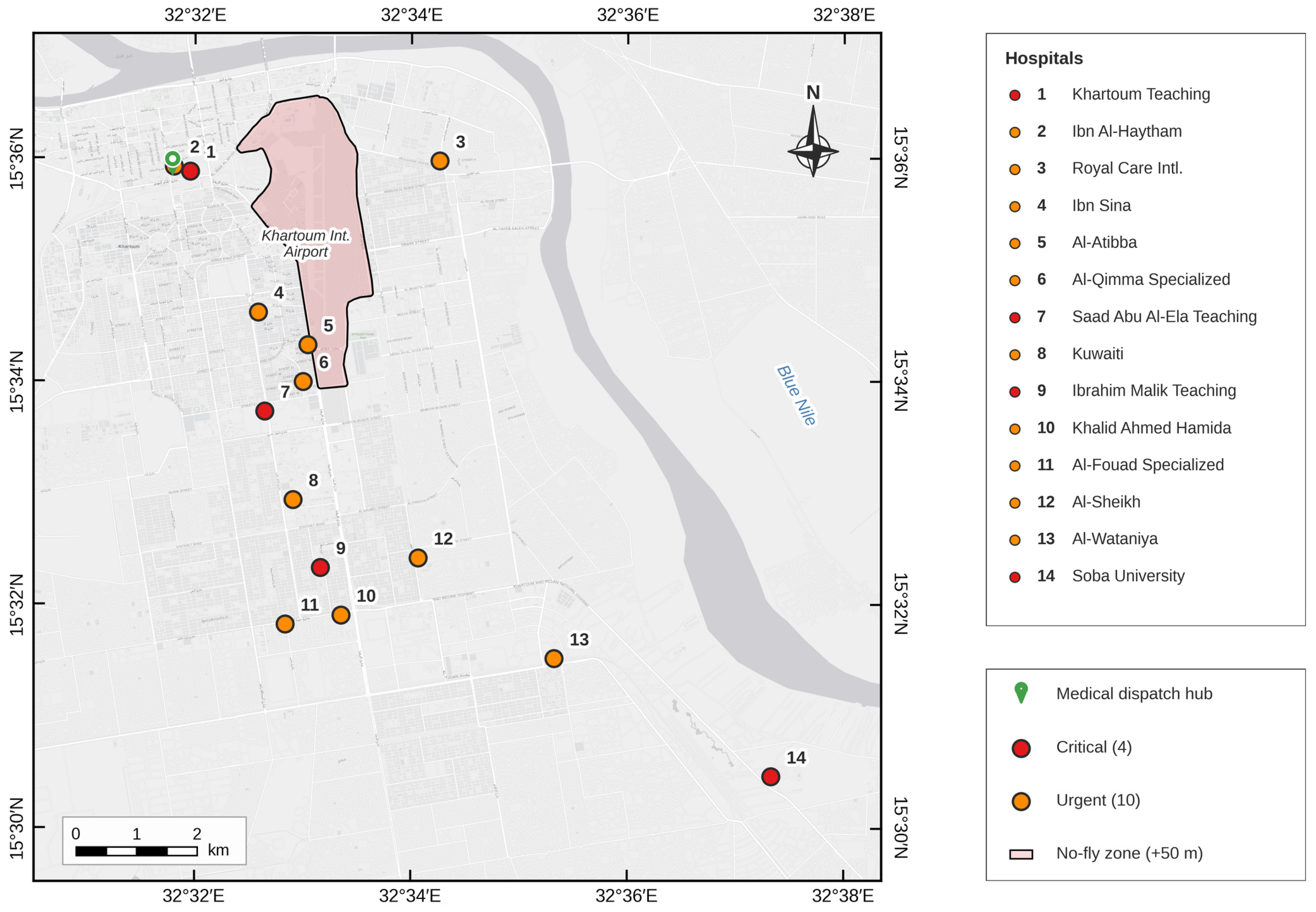
The 14-hospital evaluation network lies in Khartoum and Khartoum North, with the medical dispatch hub (central Khartoum) serving as the origin and return point for every sortie (Figure 2 and Figure 3). Under the service-based rule of Section 3.8, it contains 4 Critical hospitals (p = 1.0) and 10 Urgent hospitals (p = 0.6). The four Critical hospitals are Khartoum Teaching, Saad Abu Al-Ela Teaching, Ibrahim Malik Teaching and Soba University hospitals, all teaching or university referral hospitals with emergency services. The type of five hospitals (Ibn Al-Haytham, Al-Atibba, Kuwaiti, Khalid Ahmed Hamida and Al-Wataniya) could not be read from the name alone; the authors verified them as private multi-department inpatient hospitals, which places them in the Urgent tier. The priorities therefore describe the service level of each facility under the transparent rule of Section 3.8; they were not derived from patient-level clinical records, and no clinical data were used. Table A1 lists the attributes of the 14 hospitals. The city network contains the 59 clinical facilities of the 65-point OpenStreetMap layer. No-fly zones include Khartoum International Airport, military installations and government facilities, which every method must route around identically.

Figure 2. Study area showing the medical dispatch hub, the no-fly zone with its 50 m safety buffer, the 59 hospitals of the city network by priority tier, and the 14-hospital evaluation network (larger outlined symbols). One Urgent hospital of the city network lies 17 km south of the map frame (arrow). Panels: (a) location of Sudan and Khartoum State in Africa; (b) the seven localities of Khartoum State with the extent of the main map (red box). Graticule in degrees and minutes (WGS 84); projection WGS 84/UTM zone 36N. Basemap: Esri World Light Gray Canvas; administrative boundaries: geoBoundaries.

Figure 2. Study area showing the medical dispatch hub, the no-fly zone with its 50 m safety buffer, the 59 hospitals of the city network by priority tier, and the 14-hospital evaluation network (larger outlined symbols). One Urgent hospital of the city network lies 17 km south of the map frame (arrow). Panels: (a) location of Sudan and Khartoum State in Africa; (b) the seven localities of Khartoum State with the extent of the main map (red box). Graticule in degrees and minutes (WGS 84); projection WGS 84/UTM zone 36N. Basemap: Esri World Light Gray Canvas; administrative boundaries: geoBoundaries.

Figure 3. The 14-hospital evaluation network with rule-based priority tiers; numbers refer to the hospital list on the right. Basemap: Esri World Light Gray Canvas.

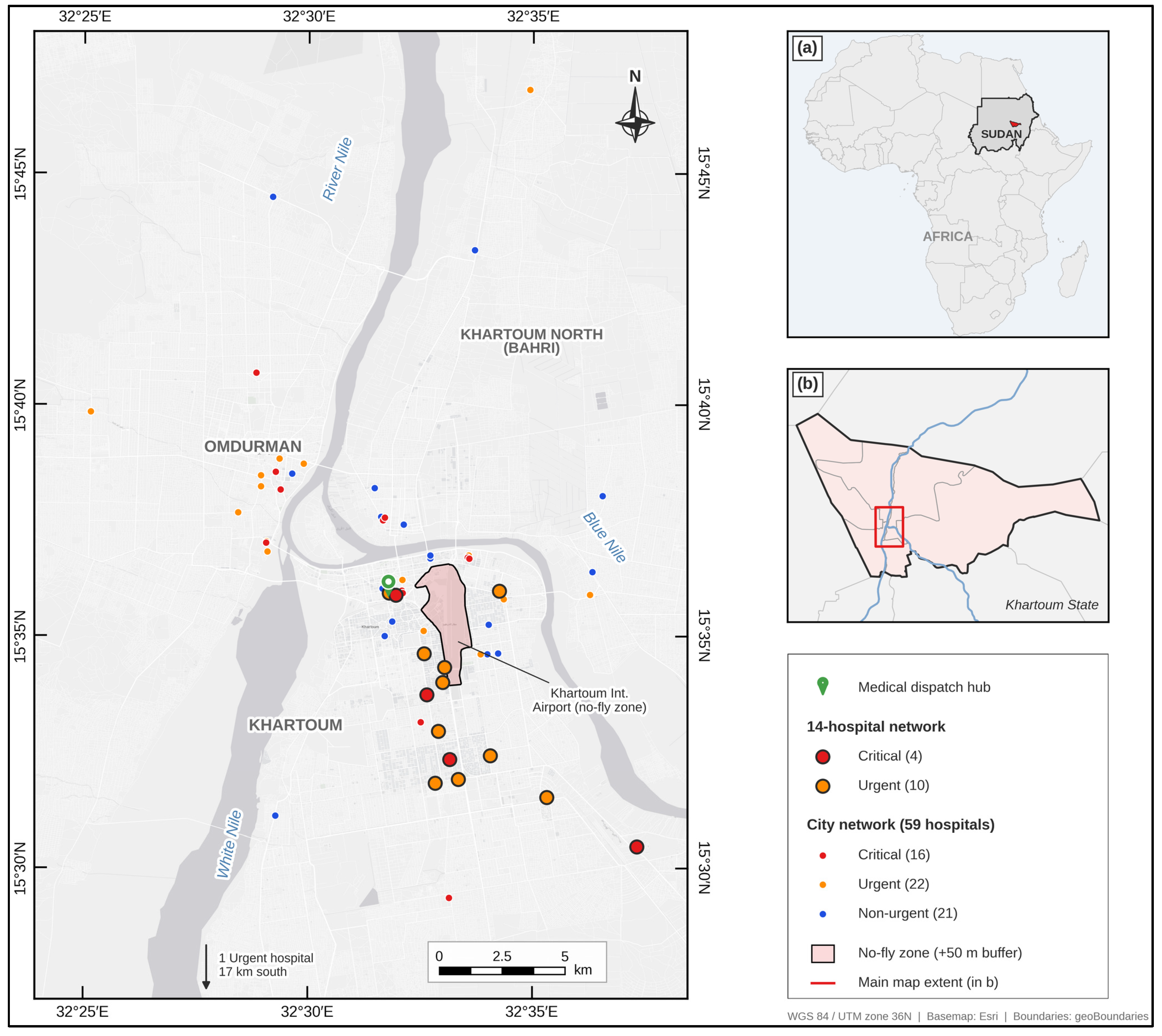
Figure 3. The 14-hospital evaluation network with rule-based priority tiers; numbers refer to the hospital list on the right. Basemap: Esri World Light Gray Canvas.

A correction was applied to the exported 14-hospital leg matrix, in which six legs (hub, Khartoum Teaching and Ibn Al-Haytham to and from Royal Care) were 3.6–3.9 km longer than the shortest obstacle-free path, because the toolbox navigation grid, sized to the extent of the input points plus a margin, did not reach around the north end of the no-fly zone. These legs were detected and replaced automatically: every exported leg is compared with the shortest obstacle-free path around the same 50 m-buffered no-fly zone, and legs more than 5% longer are replaced by that path, with the flight time recomputed by the toolbox turn-penalty model; no leg was edited by hand. To verify the correction with the method of Section 3.2, grid A* was re-run for all 210 legs on an expanded navigation domain; on this domain, the six legs measure 4.94–5.29 km instead of the exported 8.63–8.85 km, which confirms that the original grid was truncated. The corrected legs are 2.9–4.0% shorter than the expanded-grid legs, because they are not restricted to cell centres, and they run along the boundary of the 50 m buffer (minimum clearance 49.4 m from the airport polygon; 69 m for the expanded-grid legs). The selection does not depend on the 5% threshold: every other leg is within 2.9% of the obstacle-free path and the six legs are 71–80% longer, so any threshold between 3% and 70% selects the same six legs. Using the expanded-grid A* lengths for the six legs instead leaves the exact J1D optimum unchanged (same visiting order, latest Critical completion 13.0 min) and changes its distance by 0.4% (43.79 vs. 43.60 km) and its priority-weighted completion time by 0.05 min. All methods are evaluated with the same corrected matrix. All other legs agree with the obstacle-aware shortest path to within 3%.

5. Results

The results below compare three objectives. J0 is the composite cost of the previous version; it is kept only to show its flaw (Proposition 1). J1 replaces its priority term with the priority-weighted completion time, and J1D adds the hard 15 min deadline for Critical hospitals; J1D is the objective recommended for operation and the one used in the learning and city-network experiments. The methods play four distinct roles: the exact dynamic programmes provide the proven optimum against which every gap is measured; the classical heuristics (A*-DGH, A*-NN, ENN-2opt) and the metaheuristics (SA-2opt, GA) are practical baselines that run in milliseconds; OR-Tools is an independent industrial solver used as a strong external benchmark; and A2C-SP is a learned policy whose purpose is not to beat the optimum on one instance but to produce routes instantly for unseen networks, weightings and multi-sortie missions.

This approach is designed for previously unseen network configurations, objective weightings, and multi-sortie missions, rather than solely to minimise the cost of a single fixed instance.

5.1. Six-Method Comparison with Optimality Gaps

Without deadlines, 2-opt/Or-opt local search (ENN-2opt) reaches the proven optimum in 5 of the 6 J0/J1 cases (Scenarios S1-S3), so at this size local search is near-optimal on the soft objectives. With the hard deadline the picture changes: penalty-based local search can stall in infeasible local optima. The exact solution, OR-Tools and A*-NN meet the deadline in S1; SA-2opt (47% of runs) and GA (90% of runs) meet it only in some runs; ENN-2opt and A*-DGH miss it. OR-Tools, which optimises the arc-cost surrogate, is 0.9% and 12.5% above the optimum on J0 and J1, and 1.3% on J1D when time windows are added Table 10 reports the detailed results for Scenario S1.

Table 10. Priority-dominant scenario S1, 14 hospitals. Scenarios S2 and S3 are summarised in the text. Gap = (J − J*)/|J*|; for J1D over deadline-feasible runs only. Opt. hit = share of runs reaching the proven optimum; Feasible = share meeting the 15 min Critical deadline; Last Crit. = latest completion time of a covered Critical hospital; PWC = priority-weighted mean completion time.

Objective	Method	J (Mean ± s.d.)	Gap	Opt. Hit	Feasible	Dist. (km)	Last Crit. (min)	PWC (min)
J0 (published)	Exact DP	−2.5730	-	yes	0%	37.98	61.1	27.8
	OR-Tools	−2.5497	0.90%	no	0%	37.82	50.8	34.7
	ENN-2opt	−2.5730	0.00%	yes	0%	37.98	61.1	27.8
	A*-NN	−2.5730	0.00%	yes	0%	37.98	61.1	27.8
	A*-DGH	−2.0945	18.60%	no	100%	54.53	13.0	31.5
	SA-2opt	−2.5610 ± 0.0191	0.46%	30%	0%	38.23	46.0	27.2
	GA	−2.5644 ± 0.0123	0.33%	30%	0%	38.09	47.1	27.1
J1	Exact DP	2.6097	-	yes	0%	38.04	24.4	24.0
	OR-Tools	2.9347	12.45%	no	0%	37.82	50.8	34.7
	ENN-2opt	2.6097	0.00%	yes	0%	38.04	24.4	24.0
	A*-NN	2.6097	0.00%	yes	0%	38.04	24.4	24.0
	A*-DGH	2.6296	0.76%	no	0%	38.66	24.4	24.1
	SA-2opt	2.6190 ± 0.0101	0.36%	53%	0%	38.33	24.4	24.1
	GA	2.6905 ± 0.0836	3.09%	40%	0%	39.32	24.9	25.7
J1D (15 min Critical)	Exact DP	2.9731	-	yes	100%	43.60	13.0	30.6
	OR-Tools	3.0122	1.31%	no	100%	43.47	13.0	30.8
	ENN-2opt	2.8923	n/a	no	0%	41.93	15.0	29.0
	A*-NN	2.9731	0.00%	yes	100%	43.60	13.0	30.6
	A*-DGH	3.0040	n/a	no	0%	47.42	63.5	29.9
	SA-2opt	2.9311 ± 0.0485	0.11%	40%	47%	43.63	14.5	29.4
	GA	2.9813 ± 0.0455	0.55%	47%	90%	44.94	13.2	29.7
	A2C-SP zero-shot (5 seeds)	3.2610 ± 0.0262	10.08%	-	80%	53.94	13.5	29.9
	A2C-SP best-of-128	3.1117 ± 0.0900	4.66%	-	100%	49.79	13.0	29.6
	A2C-SP fine-tuned	3.0071 ± 0.0013	1.14%	-	100%	44.17	13.0	30.8

Table 10. Priority-dominant scenario S1, 14 hospitals. Scenarios S2 and S3 are summarised in the text. Gap = (J − J*)/|J*|; for J1D over deadline-feasible runs only. Opt. hit = share of runs reaching the proven optimum; Feasible = share meeting the 15 min Critical deadline; Last Crit. = latest completion time of a covered Critical hospital; PWC = priority-weighted mean completion time.

Objective	Method	J (Mean ± s.d.)	Gap	Opt. Hit	Feasible	Dist. (km)	Last Crit. (min)	PWC (min)
J0 (published)	Exact DP	−2.5730	-	yes	0%	37.98	61.1	27.8
	OR-Tools	−2.5497	0.90%	no	0%	37.82	50.8	34.7
	ENN-2opt	−2.5730	0.00%	yes	0%	37.98	61.1	27.8
	A*-NN	−2.5730	0.00%	yes	0%	37.98	61.1	27.8
	A*-DGH	−2.0945	18.60%	no	100%	54.53	13.0	31.5
	SA-2opt	−2.5610 ± 0.0191	0.46%	30%	0%	38.23	46.0	27.2
	GA	−2.5644 ± 0.0123	0.33%	30%	0%	38.09	47.1	27.1
J1	Exact DP	2.6097	-	yes	0%	38.04	24.4	24.0
	OR-Tools	2.9347	12.45%	no	0%	37.82	50.8	34.7
	ENN-2opt	2.6097	0.00%	yes	0%	38.04	24.4	24.0
	A*-NN	2.6097	0.00%	yes	0%	38.04	24.4	24.0
	A*-DGH	2.6296	0.76%	no	0%	38.66	24.4	24.1
	SA-2opt	2.6190 ± 0.0101	0.36%	53%	0%	38.33	24.4	24.1
	GA	2.6905 ± 0.0836	3.09%	40%	0%	39.32	24.9	25.7
J1D (15 min Critical)	Exact DP	2.9731	-	yes	100%	43.60	13.0	30.6
	OR-Tools	3.0122	1.31%	no	100%	43.47	13.0	30.8
	ENN-2opt	2.8923	n/a	no	0%	41.93	15.0	29.0
	A*-NN	2.9731	0.00%	yes	100%	43.60	13.0	30.6
	A*-DGH	3.0040	n/a	no	0%	47.42	63.5	29.9
	SA-2opt	2.9311 ± 0.0485	0.11%	40%	47%	43.63	14.5	29.4
	GA	2.9813 ± 0.0455	0.55%	47%	90%	44.94	13.2	29.7
	A2C-SP zero-shot (5 seeds)	3.2610 ± 0.0262	10.08%	-	80%	53.94	13.5	29.9
	A2C-SP best-of-128	3.1117 ± 0.0900	4.66%	-	100%	49.79	13.0	29.6
	A2C-SP fine-tuned	3.0071 ± 0.0013	1.14%	-	100%	44.17	13.0	30.8

Scenarios S2 and S3 lead to the same conclusions. Under J1D, the exact optimum again serves every covered Critical hospital within 13.0 min (43.43 km in S2 and 43.54 km in S3); OR-Tools and A*-NN meet the deadline in both scenarios (OR-Tools 0.76% and 2.36% above the optimum), GA meets it in 87–90% of runs and SA-2opt in 43–50%, while ENN-2opt and A*-DGH miss it. Without deadlines, ENN-2opt reaches the proven optimum in every J0 and J1 case except J0 in S3.

The stochastic methods were also compared statistically (Table A3). Over 30 seeds on S1, SA-2opt and GA do not differ significantly under J0 (Mann–Whitney U test, p = 0.73); SA-2opt is closer to the optimum under J1 (p = 0.004); under J1D, GA meets the deadline significantly more often than SA-2opt (90% vs. 47% of runs, Fisher exact test, p < 0.001), while their penalised objectives do not differ significantly (p = 0.06). On the 47 held-out instances (Wilcoxon signed-rank test, paired by instance), ENN-2opt is significantly closer to the optimum than GA (p < 0.001), and both are significantly better than the zero-shot A2C-SP with greedy or best-of-128 decoding (p < 10⁻⁹). Bootstrap 95% confidence intervals of the mean gaps and Wilson intervals of the feasibility rates are given in Table A3.

When re-scored on the corrected model, the previously published learned-policy route for S1 measures 45.55 km and 70.4 min (published: 49.97 km, 97.8 min). It is 7.1% above the J0 optimum and 26.5% above the J1 optimum.

5.2. A2C-SP Training and Generalisation

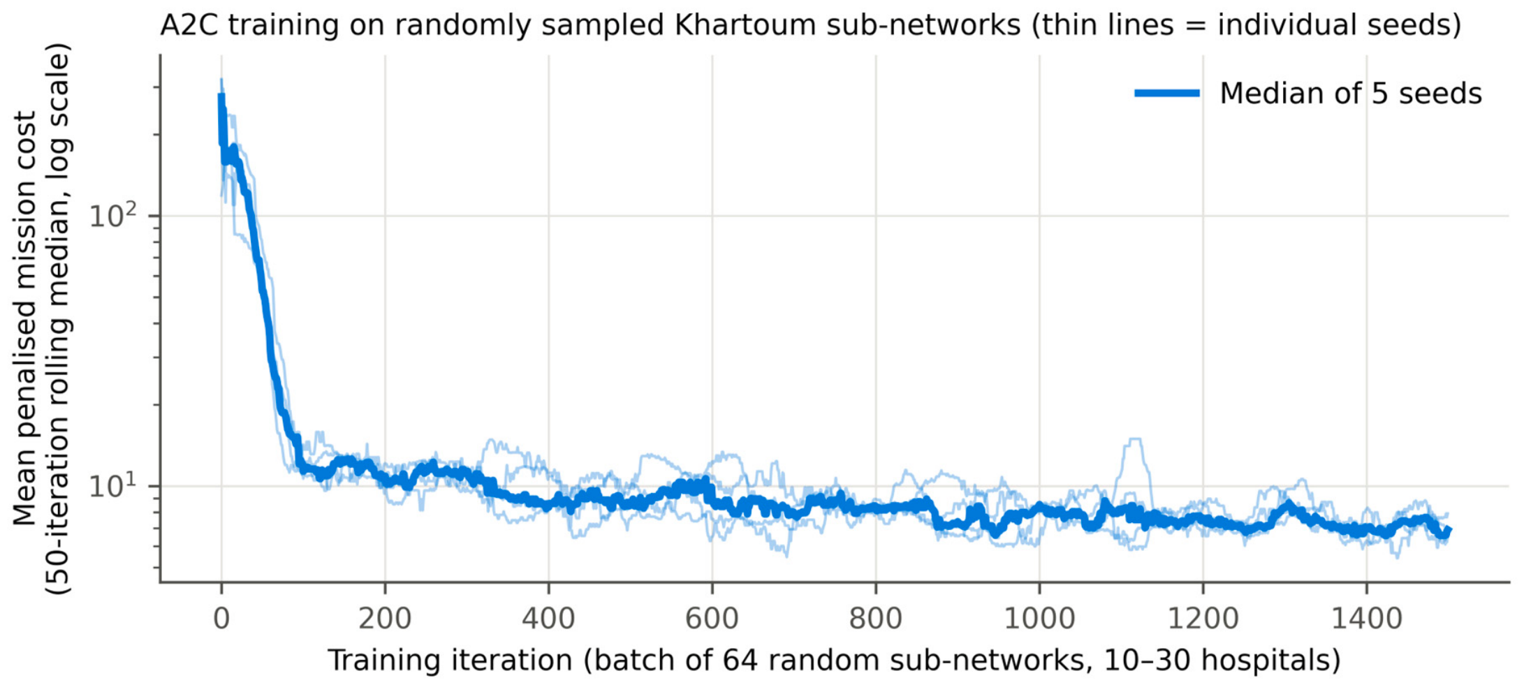
The policy is not optimal (Table 11). Zero-shot, it is 14.7% above the optimum on unseen sub-networks and 10.1% on the unseen 14-hospital network, and fine-tuning reduces the latter to 1.1%. Zero-shot, 4 of the 5 seeds meet the Critical deadline (S1); after fine-tuning, 5 of 5 do. With the full training budget, the original learning rate (3 × 10⁻⁴) performs similarly (Section 5.3). Its value lies in speed and in generality (unseen networks, arbitrary weights, multi-sortie missions), not in beating local search on a 14-hospital instance, Figure 4 shows the training curves of the five seeds.

Table 11. Generalisation of A2C-SP under J1D (15 min Critical deadline), S1 weights. The optimum is known exactly for every instance (label-setting DP). Run times on the 14-hospital network are medians over the five seeds (the first call of a session adds about 2 s of start-up time).

Test Set	Decoding	Mean Gap to Optimum	s.d. over 5 Seeds	Instances Within 1%	Time per Instance
47 held-out sub-networks	A2C-SP greedy	14.7%	6.8%	5%	1.7 ms
	A2C-SP best-of-128	8.8%	4.2%	8%	273 ms
	ENN-2opt	0.81%	-	81%	6.9 ms
	GA (1 run)	2.07%	-	47%	57 ms
14-hospital network (unseen), S1	A2C-SP greedy	10.1%	0.0	-	18 ms
	A2C-SP best-of-128	4.7%	3.0	-	189 ms
	A2C-SP fine-tuned (300 it.)	1.1%	0.0	-	59 s

Table 11. Generalisation of A2C-SP under J1D (15 min Critical deadline), S1 weights. The optimum is known exactly for every instance (label-setting DP). Run times on the 14-hospital network are medians over the five seeds (the first call of a session adds about 2 s of start-up time).

Test Set	Decoding	Mean Gap to Optimum	s.d. over 5 Seeds	Instances Within 1%	Time per Instance
47 held-out sub-networks	A2C-SP greedy	14.7%	6.8%	5%	1.7 ms
	A2C-SP best-of-128	8.8%	4.2%	8%	273 ms
	ENN-2opt	0.81%	-	81%	6.9 ms
	GA (1 run)	2.07%	-	47%	57 ms
14-hospital network (unseen), S1	A2C-SP greedy	10.1%	0.0	-	18 ms
	A2C-SP best-of-128	4.7%	3.0	-	189 ms
	A2C-SP fine-tuned (300 it.)	1.1%	0.0	-	59 s

Figure 4. A2C-SP training: mean penalised mission cost per batch of 64 random sub-networks (50-iteration rolling median, log scale); thin lines are the 5 seeds.

Figure 4. A2C-SP training: mean penalised mission cost per batch of 64 random sub-networks (50-iteration rolling median, log scale); thin lines are the 5 seeds.

5.3. Hyperparameter Sensitivity

The learning rate dominates (Table 12): at a 300-iteration budget, 10⁻³ is clearly best and 10⁻⁴ leaves every seed under-trained. The entropy coefficient matters less and is not monotonic. The selected configuration (10⁻³, 0) was retrained for the full budget with 5 new seeds. At the full budget, the original learning rate 3 × 10⁻⁴ gives a zero-shot gap of 13.8% on the 14-hospital network.

Table 12. Multi-seed sensitivity: 3 × 3 configurations × 5 seeds (45 runs, 300 iterations each), ranked on a validation set disjoint from the test set.

Learning Rate	Entropy Coef.	Mean Validation Gap	s.d. over Seeds	Best Seed	Worst Seed
1 × 10−3	0.0	20.5%	11.5%	11.9%	37.8%
1 × 10−3	0.05	24.9%	14.4%	12.6%	42.0%
1 × 10−3	0.01	33.2%	15.7%	16.7%	53.2%
3 × 10−4	0.01	56.7%	18.6%	29.0%	71.8%
3 × 10−4	0.05	59.0%	30.6%	22.1%	102.6%
3 × 10−4	0.0	66.6%	28.9%	22.5%	103.8%
1 × 10−4	0.05	76.9%	33.0%	31.1%	116.9%
1 × 10−4	0.0	84.3%	21.7%	64.3%	108.5%
1 × 10−4	0.01	85.5%	23.9%	64.7%	115.1%

5.4. ArcGIS/Offline Round-Trip Verification

The two computations, one performed entirely in the offline training script from the Pairwise Leg Matrix and the other entirely in ArcGIS Pro’s path-geometry and cost engine after importing the policy’s visiting order in Predefined-Sequence mode, agree to within 4 × 10⁻⁷ in composite cost for every scenario (Table 13). The two pipelines were built independently from the same equations, and their agreement is demonstrated rather than assumed. The same check was extended to the complete evaluator used in this revision: re-computing every exported ArcGIS Pro run from the Pairwise Leg Matrices reproduces the ArcGIS distances and times with maximum residuals of 1 × 10⁻¹⁰ m and 4 × 10⁻¹² s (23 exported runs, both networks; Supplementary Materials).

Table 13. Agreement between the externally trained policy’s own cost computation and ArcGIS Pro’s re-computation of the same route (previous version).

Scenario	Offline Training-Script Cost	ArcGIS Predefined-Sequence Cost	Absolute Difference
Scenario 1	−1.162904	−1.162904	2 × 10−7
Scenario 2	1.609631	1.609631	3.91 × 10−7
Scenario 3	1.037683	1.037683	3.59 × 10−7

Table 13. Agreement between the externally trained policy’s own cost computation and ArcGIS Pro’s re-computation of the same route (previous version).

Scenario	Offline Training-Script Cost	ArcGIS Predefined-Sequence Cost	Absolute Difference
Scenario 1	−1.162904	−1.162904	2 × 10−7
Scenario 2	1.609631	1.609631	3.91 × 10−7
Scenario 3	1.037683	1.037683	3.59 × 10−7

5.5. Clinical Priority Compliance: Completion-Time Analysis

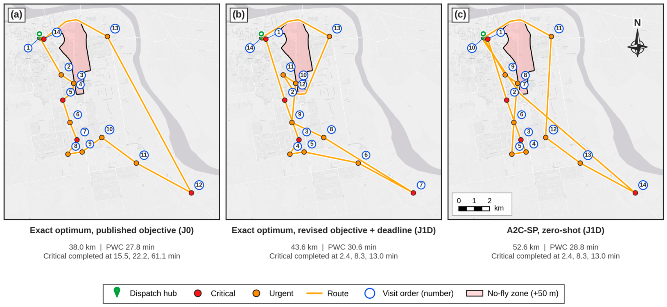
Under J0, every whole-tour optimiser (exact, ENN-2opt, SA-2opt, GA, OR-Tools) serves at least one covered Critical hospital after 46 min (Figure 5). This is Proposition 1 at work: the priority term cancels over the tour. Only the one-step greedy A*-DGH serves them early, because for a single leg −w₄p_j is not constant, and with w₄ = 0.45 it outweighs the distance and time of nearby candidates. That behaviour is an artefact of myopia: A*-DGH is 19% above the J0 optimum and fails the deadline once the objective is corrected. The previous learned policy, whose return equalled the total tour cost, behaved like a whole-tour optimiser and was further penalised by the altitude error. Under J1D the exact optimum serves every covered Critical hospital within 13.0 min (Figure 5 and Figure 6).

Figure 5. Completion time of the four Critical hospitals (S1) under the published objective (left) and the revised objective with the 15 min deadline (right, dashed line). Soba University Hospital lies outside the 15 min direct-flight coverage and is exempted from the deadline.

Figure 5. Completion time of the four Critical hospitals (S1) under the published objective (left) and the revised objective with the 15 min deadline (right, dashed line). Soba University Hospital lies outside the 15 min direct-flight coverage and is exempted from the deadline.

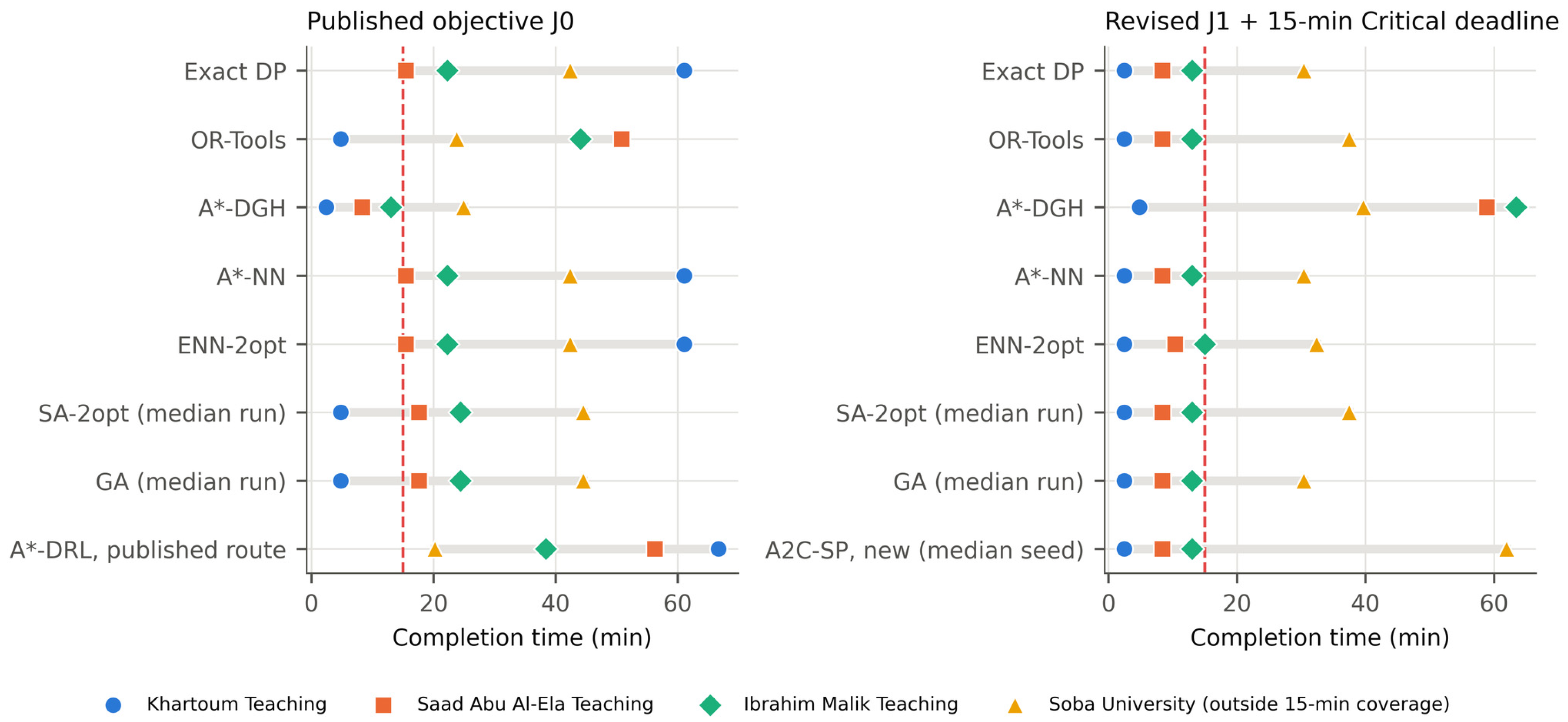
Figure 6. 14-hospital network, S1: exact optimum under the published objective (a), exact optimum under the revised objective with the deadline (b), and the zero-shot A2C-SP (c). Numbers give the visiting order; the green pin marks the dispatch hub. Basemap: Esri World Light Gray Canvas.

Figure 6. 14-hospital network, S1: exact optimum under the published objective (a), exact optimum under the revised objective with the deadline (b), and the zero-shot A2C-SP (c). Numbers give the visiting order; the green pin marks the dispatch hub. Basemap: Esri World Light Gray Canvas.

5.6. Robustness to Weights, Deadlines and Elevation Error

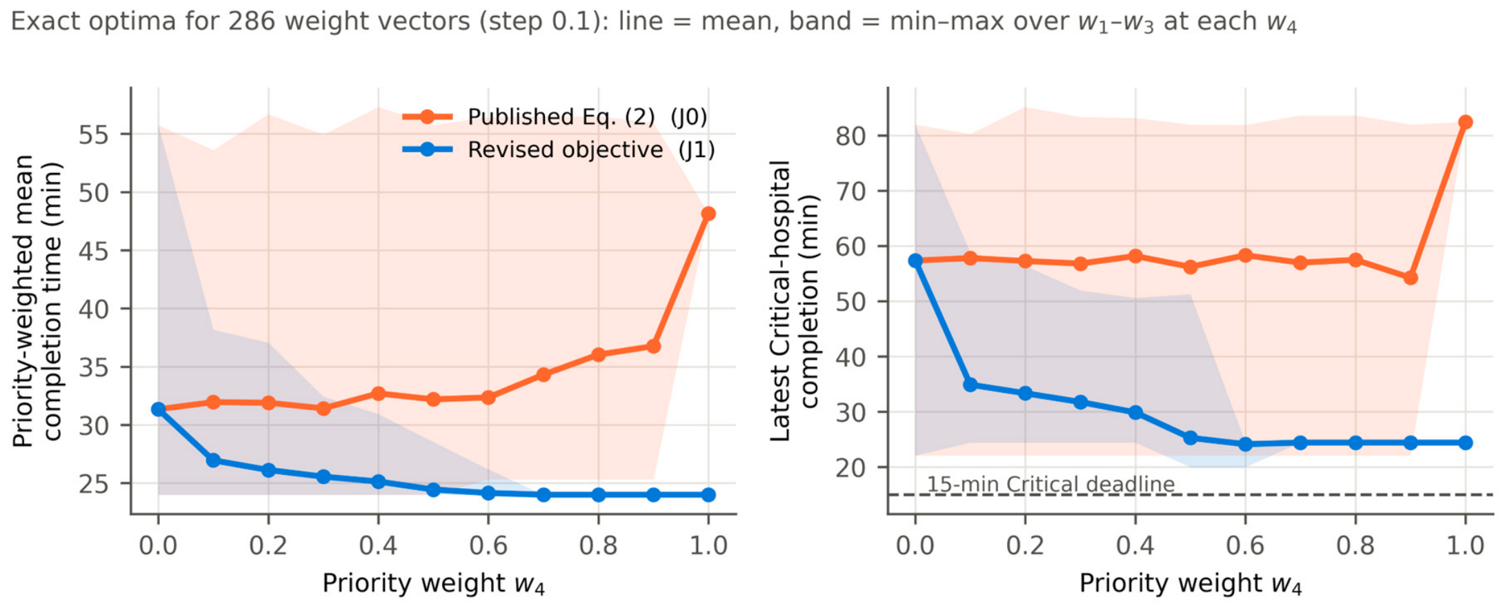
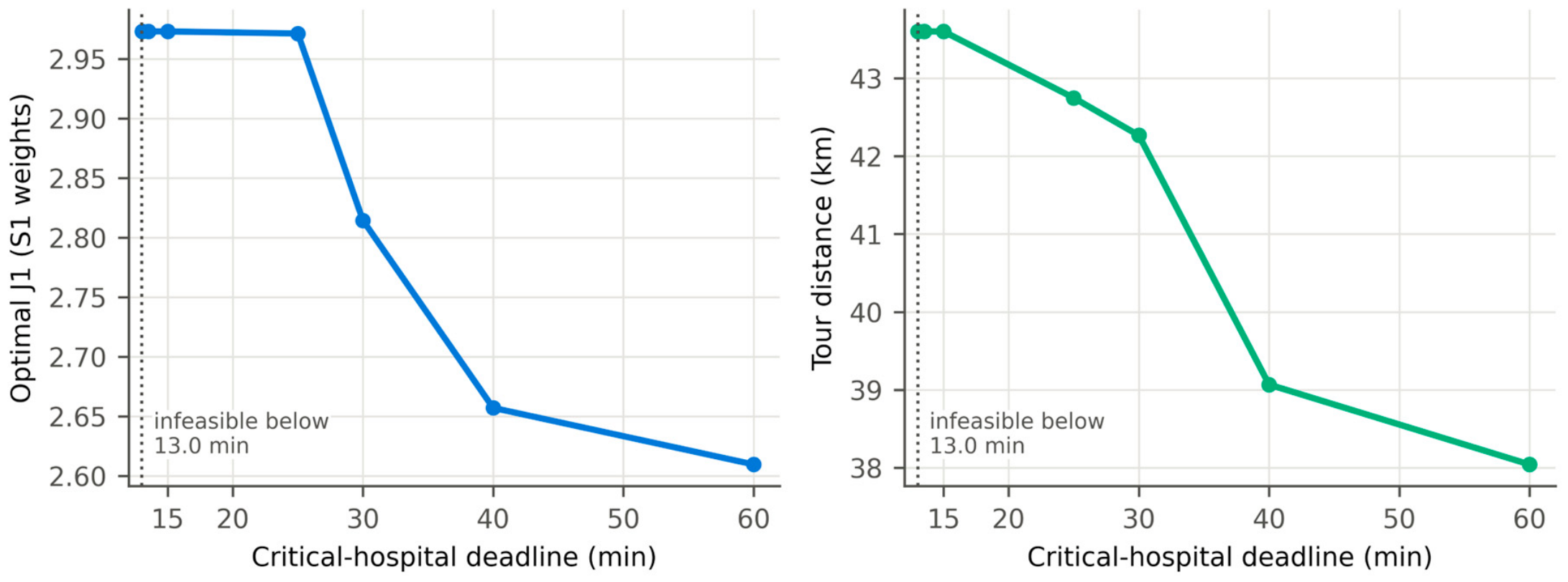
Under J0 the priority-weighted completion time of the optimum is 32.1 min on average and does not improve as w₄ grows (Figure 7). Under J1 it falls to 25.2 min on average for any w₄ ≥ 0.2, whatever w₁–w₃ are. The main conclusions therefore do not depend on the exact panel judgements. No weighting of J1 alone guarantees the 15 min deadline, which is why Equation (4) is needed. Figure 8 shows the corresponding price of priority: tightening the Critical deadline from 60 min to 13.0 min raises the optimal tour distance from 38.04 km to 43.60 km.

Figure 7. Exact optima for 286 weight vectors: priority-weighted mean completion time (left) and latest Critical completion (right) as a function of w₄.

Figure 7. Exact optima for 286 weight vectors: priority-weighted mean completion time (left) and latest Critical completion (right) as a function of w₄.

The flat-terrain assumption does not change the optimal route. With elevation errors of 5–20 m, the optimal cost changes by at most 4.8%, and where the re-optimised route differs, the nominal route is at most 3.2% worse and still meets the deadline in every draw. Route changes occur because the optimum serves a Critical hospital within seconds of the deadline, so small timing shifts decide whether one extra stop fits before it. The conclusions are therefore robust to GNSS elevation error (Table 14). Operational parameters (Table A2). On the 14-hospital network the three covered Critical hospitals keep the same order (Khartoum Teaching, Saad Abu Al-Ela, Ibrahim Malik) and are all completed within 15 min for every cruise speed between 15 and 23 m/s, service time between 30 and 90 s and cruise altitude between 350 and 410 m AMSL. The optimal route is unchanged for slower flight, longer service and a higher cruise altitude; with faster flight (20–23 m/s) or a lower cruise altitude (350 m), the only change is that Ibn Sina is visited second, and with a 30 s service time Ibn Al-Haytham is visited first and Ibn Sina third, because shorter legs leave time for nearby Urgent stops before the deadline. With a 120 s service time the 15 min deadline becomes infeasible, and the earliest achievable latest Critical completion is 16.0 min. With faster flight, a 30 s service time or a 350 m cruise altitude, Soba University Hospital falls inside the 15 min direct-flight coverage; a single UAV could then serve all four Critical hospitals only by 20.1–21.8 min, which again points to fleet or hub planning rather than routing. On the city network, payload capacity (4–8 kg) and range (60–200 km) change the number of sorties as expected (3.0–8.6 on average), but the number of Critical deadline misses stays at 11–12 of 16 in every case, because the bound of Section 5.7 is set by the geography rather than by capacity or range.

Table 14. Sensitivity of the exact J1D optimum (S1) to GNSS elevation error (Gaussian noise on every node) and to a flat-terrain assumption J* = optimal objective value.

Elevation Model	Draws	Optimal Route Unchanged	Max|Change|in J* (%)	Max Regret of Nominal Route (%)	Nominal Route Still Meets Deadline
flat terrain	1	100%	0.37	0.00	100%
sigma = 5 m	20	60%	3.17	2.87	100%
sigma = 10 m	20	65%	3.37	2.97	100%
sigma = 20 m	20	50%	4.84	3.17	100%

Table 14. Sensitivity of the exact J1D optimum (S1) to GNSS elevation error (Gaussian noise on every node) and to a flat-terrain assumption J* = optimal objective value.

Elevation Model	Draws	Optimal Route Unchanged	Max|Change|in J* (%)	Max Regret of Nominal Route (%)	Nominal Route Still Meets Deadline
flat terrain	1	100%	0.37	0.00	100%
sigma = 5 m	20	60%	3.17	2.87	100%
sigma = 10 m	20	65%	3.37	2.97	100%
sigma = 20 m	20	50%	4.84	3.17	100%

Figure 8. Price of priority: optimal J1 and tour distance as the Critical deadline is tightened (S1). Deadlines below 13.0 min are infeasible.

Figure 8. Price of priority: optimal J1 and tour distance as the Critical deadline is tightened (S1). Deadlines below 13.0 min are infeasible.

5.7. City Network (59 Hospitals) with Capacity and Range

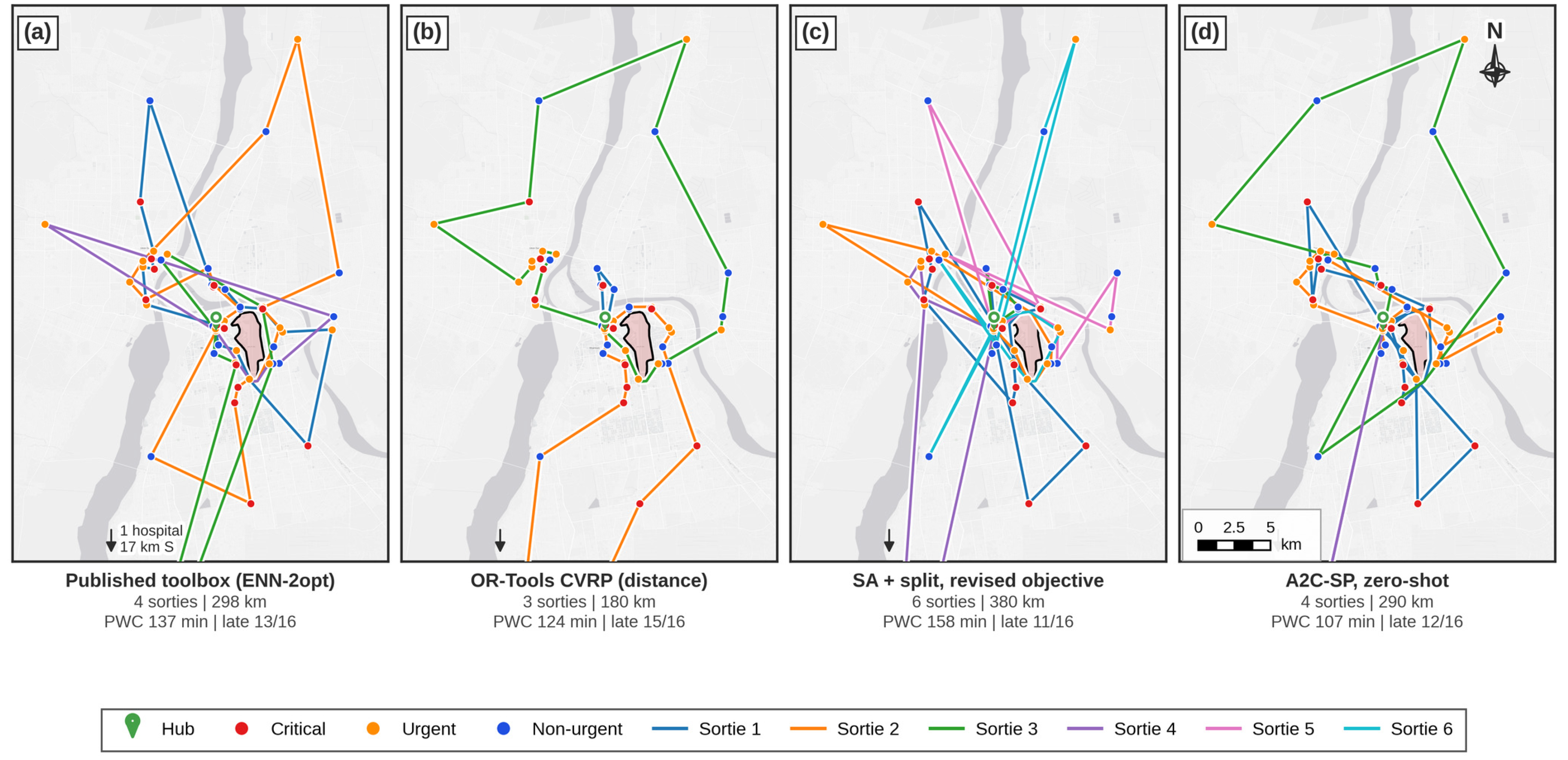
An exhaustive enumeration over every subset and order of the Critical hospitals shows that no single-UAV route can serve more than 5 of the 16 Critical hospitals within 15 min, even with lower-bound travel times that allow any intermediate stops and ignore payload. At least 11 misses are therefore unavoidable, and meeting the deadline at city scale requires a second UAV or a second hub (Section 6.4). Without retraining, the A2C-SP plans capacity- and range-feasible missions of 4.0 sorties and 287 km on average over the five seeds Figure 9. This removes the 7-sortie, 541 km failure of the previous version, and its priority-weighted completion time (110 min) is the lowest in Table 15. The distance-optimal OR-Tools CVRP is much shorter (180 km) but ignores priority (priority-weighted completion 124 min). This illustrates the efficiency-priority trade-off at city scale.

Table 15. City network (59 hospitals, rule-based priorities), S1 weights, 6 kg capacity, 100 km per sortie, 15 min Critical deadline. Published routes are re-scored on the same 3-D model.

Method	Sorties	J1	Dist. (km)	Mission (h)	Crit. Misses (of 16)	Last Crit. (min)	PWC (min)	Run Time
Published ENN-2opt (toolbox split)	4.0	7.041	298	6.50	13.0	329.8	136.8	-
Published A*-NN	4.0	7.062	299	6.52	13.0	331.2	138.0	-
Published GA	4.0	7.130	304	6.60	15.0	336.1	141.4	-
Published A*-DGH	4.0	7.500	375	7.62	15.0	401.2	171.5	-
Published learned policy	7.0	8.788	541	10.21	16.0	579.3	267.5	-
OR-Tools CVRP (distance)	3.0	6.235	180	4.74	15.0	215.5	124.0	60.06 s
SA giant tour + split (5 seeds)	5.6	6.509	365	7.53	11.4	85.8	155.3	0.78 s
A2C-SP zero-shot, greedy (5 seeds)	4.0	6.975	287	6.36	12.0	151.6	110.1	0.13 s
A2C-SP zero-shot, best-of-128 (5 seeds)	4.2	7.234	320	6.86	12.0	147.6	118.0	3.40 s

Figure 9. Sorties on the city network: (a) published toolbox route, (b) distance-optimal OR-Tools CVRP, (c) priority-aware simulated annealing, and (d) zero-shot A2C-SP. Legs are drawn along obstacle-aware paths around the buffered no-fly zone; colours distinguish sorties. Basemap: Esri World Light Gray Canvas. One Urgent hospital lies 17 km south of the frame (arrow); legs to it leave the frame at the bottom.

Figure 9. Sorties on the city network: (a) published toolbox route, (b) distance-optimal OR-Tools CVRP, (c) priority-aware simulated annealing, and (d) zero-shot A2C-SP. Legs are drawn along obstacle-aware paths around the buffered no-fly zone; colours distinguish sorties. Basemap: Esri World Light Gray Canvas. One Urgent hospital lies 17 km south of the frame (arrow); legs to it leave the frame at the bottom.

6. Discussion

6.1. Interpreting the Comparative Results

Three findings stand out. First, the objective matters more than the algorithm: with the published composite cost, every whole-tour optimiser defers at least one Critical hospital, because the priority term is identical for every complete tour (Proposition 1); with the priority-weighted completion time and a deadline, the optimal route serves every covered Critical hospital within 13.0 min at a small cost in distance. Second, with proven optima as the yardstick, 2-opt/Or-opt local search is near-optimal on a 14-hospital mission with soft objectives, but penalty-based local search and metaheuristics can stall in infeasible local optima once hard deadlines are imposed, whereas exact dynamic programming and OR-Tools with time windows respect them. Third, the learned policy is not the most accurate method at this size; its advantages are that it is trained once, produces a route in milliseconds, accepts any weighting of the criteria and handles payload and range constraints on unseen networks, where the previous version failed. The dynamic-payload model remains the physically realistic choice, because the payload on board changes the effective speed and hence the completion times that the revised objective measures.

6.2. Computational Complexity and Measured Runtime

Exact dynamic programming grows as 2n and is practical up to about 25 hospitals per sortie, which covers the single-UAV missions considered here; beyond that, local search, OR-Tools and the learned policy scale polynomially. The learned policy has the highest one-off cost (training) but the lowest cost per new mission (Table 16).

Table 16. Asymptotic complexity and measured run times (Python, 2 CPU cores).

Method	Complexity	Measured, 14 Hospitals	Measured, 59 Hospitals
Leg matrix (grid A*)	O(n2 G log G)	shared, one-off	shared, one-off (about 4 min in ArcGIS Pro)
Exact DP/label DP	O(2n n2)	0.3–0.6 s	intractable
A*-DGH	O(n2)	<1 ms	-
A*-NN/ENN-2opt	O(n2) per pass	3/6 ms	-
SA-2opt/GA	O(I n)/O(G P n)	42/69 ms	0.8 s (SA)
OR-Tools	time-limited	10 s	60 s
A2C-SP inference	O(n3 d) per tour	18 ms (greedy, median)	0.13 s greedy/3.4 s best-of-128
A2C-SP training	O(iterations × B × n3 d)	12–20 min per seed (2 CPU cores), once for all networks

Table 16. Asymptotic complexity and measured run times (Python, 2 CPU cores).

Method	Complexity	Measured, 14 Hospitals	Measured, 59 Hospitals
Leg matrix (grid A*)	O(n2 G log G)	shared, one-off	shared, one-off (about 4 min in ArcGIS Pro)
Exact DP/label DP	O(2n n2)	0.3–0.6 s	intractable
A*-DGH	O(n2)	<1 ms	-
A*-NN/ENN-2opt	O(n2) per pass	3/6 ms	-
SA-2opt/GA	O(I n)/O(G P n)	42/69 ms	0.8 s (SA)
OR-Tools	time-limited	10 s	60 s
A2C-SP inference	O(n3 d) per tour	18 ms (greedy, median)	0.13 s greedy/3.4 s best-of-128
A2C-SP training	O(iterations × B × n3 d)	12–20 min per seed (2 CPU cores), once for all networks

6.3. Comparative Positioning Relative to Prior Literature

Table 1 (Section 2.6) situates this study against the operational UAV-delivery studies and the learning-based and metaheuristic routing studies discussed earlier. Operational studies [2,4,6] demonstrate the value of medical drones but do not optimise multi-stop sequences; learning-based routing studies [19,22,26,27] rarely report optimality gaps against proven optima on real obstacle-aware networks.

To the authors’ knowledge, this study is among the few that benchmark a trained actor–critic sequencing policy against constructive heuristics, local search and population-based metaheuristics simultaneously, on the same obstacle-aware spatial infrastructure and the same explicit multi-criteria objective, with criteria weights elicited from health professionals, proven optima as the yardstick, hard clinical deadlines and multi-seed reporting for the trained policy.

6.4. Limitations

Several limitations should be noted. Proven optima are available only up to about 25 hospitals; for the city network we therefore report the best solutions found and an enumeration bound on Critical deadline compliance, not a certified optimum. In addition, the learned policy remains 10–15% above the optimum in the zero-shot setting and is outperformed by 2-opt/Or-opt local search at 14 hospitals. The leg model does not include wind, battery state of charge, ground turnaround time between sorties or dynamic airspace (NOTAM) updates. Moreover, the AHP weights come from a single-city panel of 10 health professionals, and the 15 min deadline is a service target rather than a clinical threshold; both are tested by sensitivity analyses, but a larger multi-centre panel would strengthen them. Finally, the analysis assumes one UAV and one hub, and the city-network results show that a deadline guarantee at city scale is a fleet- and hub-location problem.

7. Conclusions and Future Work

A linear priority term in a composite tour cost cannot express clinical urgency, because it is identical for every complete tour. A priority-weighted completion-time objective with hard deadlines can, and on the Khartoum network it reduces the priority-weighted completion time of the optimal route by 14% with 0.2% more distance, with all Critical hospitals within the hub’s coverage served within 15 min when the deadline is imposed. With proven optima as the yardstick, 2-opt/Or-opt local search is near-optimal for a 14-hospital mission on soft objectives, and a size-invariant A2C sequencing policy trained once on random sub-networks is within about 15% of optimal on unseen instances, needs milliseconds per route, and plans feasible multi-sortie missions on the 59-hospital city network. At city scale, deadline compliance is limited by fleet size rather than by the routing algorithm.

All methods are available as parameter choices in a single ArcGIS Pro Python toolbox, which includes a Pairwise Leg Matrix export and a Predefined-Sequence import, so that an externally trained policy is re-scored inside ArcGIS Pro with the same geometry engine as every classical algorithm. Because the complete evaluator is also implemented in Python, every result can be reproduced from the exported leg matrices.

Future work should address a larger multi-centre panel of clinicians for the weights and deadlines; multi-UAV and multi-hub dispatch, for which the city-network bound shows the need; and energy- and wind-aware leg models with dynamic no-fly-zone updates.

References

- United Nations Office for the Coordination of Humanitarian Affairs (OCHA). Sudan Humanitarian Needs Overview 2023; OCHA: New York, NY, USA, 2022; Available online: https://reliefweb.int/report/sudan/sudan-humanitarian-needs-overview-2023-november-2022 (accessed on 23 August 2026).
- Nisingizwe, M.P.; Ndishimye, P.; Swaibu, K.; Nshimiyimana, L.; Karame, P.; Dushimiyimana, V.; Musabyimana, J.P.; Musanabaganwa, C.; Nsanzimana, S.; Law, M.R. Effect of unmanned aerial vehicle (drone) delivery on blood product delivery time and wastage in Rwanda: A retrospective, cross-sectional study and time series analysis. Lancet Glob. Health 2022, 10, e564–e569. [Google Scholar] [CrossRef] [Scilit]
- Hart, P.E.; Nilsson, N.J.; Raphael, B. A formal basis for the heuristic determination of minimum cost paths. IEEE Trans. Syst. Sci. Cybern. 1968, 4, 100–107. [Google Scholar] [CrossRef] [Scilit]
- Haidari, L.A.; Brown, S.T.; Ferguson, M.; Bancroft, E.; Spiker, M.; Wilcox, A.; Ambikapathi, R.; Sampath, V.; Connor, D.L.; Lee, B.Y. The economic and operational value of using drones to transport vaccines. Vaccine 2016, 34, 4062–4067. [Google Scholar] [CrossRef] [Scilit]
- Scott, J.E.; Scott, C.H. Drone delivery models for healthcare. In Proceedings of the 50th Hawaii International Conference on System Sciences (HICSS-50), Hilton Waikoloa Village, HI, USA, 4–7 January 2017; pp. 3297–3304. Available online: https://aisel.aisnet.org/hicss-50/hc/global_health/7/ (accessed on 23 August 2026).
- Boutilier, J.J.; Chan, T.C.Y. Drone network design for cardiac arrest response. Manuf. Serv. Oper. Manag. 2022, 24, 2407–2424. [Google Scholar] [CrossRef] [Scilit]
- Gugan, G.; Haque, A. Path planning for autonomous drones: Challenges and future directions. Drones 2023, 7, 169. [Google Scholar] [CrossRef] [Scilit]
- Abdelrhman, A.; Damos, M.A.; Dafallah, M. Multi Criteria GIS Optimization of Emergency Medical Supply Routes in Khartoum: A Comparative Study of Drone and Road Transport Using Advanced Pathfinding Algorithms. J. Karary Univ. Eng. Sci. 2026, 5, 1–12. Available online: https://journals.karary.edu.sd/index.php/JKUES/article/view/443 (accessed on 17 October 2026). [CrossRef]
- Borja-Jaimes, V.; Valdez-Martínez, J.S.; Beltrán-Escobar, M.; Ramírez-Zúñiga, G.; Reyes-Mayer, A.; Calixto-Rodríguez, M. Robust Backstepping-Sliding Control of a Quadrotor UAV with Disturbance Compensation. Computation 2026, 14, 51. [Google Scholar] [CrossRef] [Scilit]
- Espinosa Pedroza, A.D.; Vazquez Trejo, J.A.; Ortiz-Torres, G.; Alonso-Bastida, A.; Rios-Enriquez, C.; Peregrino, C.A.; Adam-Medina, M. Leader-following consensus control robust to external disturbances for LPV multi-agent systems. Asian J. Control 2025, 28, 2165–2178. [Google Scholar] [CrossRef] [Scilit]
- Dijkstra, E.W. A note on two problems in connexion with graphs. Numer. Math. 1959, 1, 269–271. [Google Scholar] [CrossRef] [Scilit]
- Thiels, C.A.; Aho, J.M.; Zietlow, S.P.; Jenkins, D.H. Use of unmanned aerial vehicles for medical product transport. Air Med. J. 2015, 34, 104–108. [Google Scholar] [CrossRef] [Scilit]
- Hii, M.S.Y.; Courtney, P.; Royall, P.G. An evaluation of the delivery of medicines using drones. Drones 2019, 3, 52. [Google Scholar] [CrossRef] [Scilit]
- Held, M.; Karp, R.M. A dynamic programming approach to sequencing problems. J. Soc. Ind. Appl. Math. 1962, 10, 196–210. [Google Scholar] [CrossRef] [Scilit]
- Miller, C.E.; Tucker, A.W.; Zemlin, R.A. Integer programming formulation of traveling salesman problems. J. ACM 1960, 7, 326–329. [Google Scholar] [CrossRef] [Scilit]
- Solomon, M.M. Algorithms for the vehicle routing and scheduling problems with time window constraints. Oper. Res. 1987, 35, 254–265. [Google Scholar] [CrossRef] [Scilit]
- Arce-Ortega, D.V.; Alonso-Pecina, F.; Cruz-Chávez, M.A.; Peralta-Abarca, J.d.C. A Simulated Annealing Approach for the Homogeneous Capacitated Vehicle Routing Problem. Mathematics 2025, 13, 3209. [Google Scholar] [CrossRef] [Scilit]
- Perron, L.; Furnon, V. OR-Tools (v9.15); Google: Mountain View, CA, USA, 2026; Available online: https://developers.google.com/optimization/ (accessed on 21 August 2026).
- Li, Y.; Guan, Q.; Gu, J.; Jiang, X. A deep reinforcement learning with dynamic spatio-temporal graph model for solving urban logistics delivery planning problems. Int. J. Digit. Earth 2024, 17, 2376273. [Google Scholar] [CrossRef] [Scilit]
- Liu, M.; Demir, E.; Jian, L. Reinforcement learning for the vehicle routing problem: Methodologies, applications, and research outlook. Arab. J. Sci. Eng. 2026, 51, 6497–6524. [Google Scholar] [CrossRef] [Scilit]
- Martins, M.S.E.; Sousa, J.M.C.; Vieira, S. A systematic review on reinforcement learning for industrial combinatorial optimization problems. Appl. Sci. 2025, 15, 1211. [Google Scholar] [CrossRef] [Scilit]
- Taresh, A.A.R.; Asgharian Sardroud, A.A.; Tajbakhsh, M.S. Solving the traveling salesman problem with drones using proximal policy optimization and deep reinforcement learning. J. Inf. Syst. Eng. Manag. 2025, 10, 1414–1423. [Google Scholar] [CrossRef] [Scilit]
- Williams, R.J. Simple statistical gradient-following algorithms for connectionist reinforcement learning. Mach. Learn. 1992, 8, 229–256. [Google Scholar] [CrossRef] [Scilit]
- Mnih, V.; Badia, A.P.; Mirza, M.; Graves, A.; Lillicrap, T.; Harley, T.; Silver, D.; Kavukcuoglu, K. Asynchronous methods for deep reinforcement learning. In Proceedings of the 33rd International Conference on Machine Learning (ICML 2016), New York, NY, USA, 19–24 June 2016; Volume PMLR 48, pp. 1928–1937. Available online: https://proceedings.mlr.press/v48/mniha16.html (accessed on 23 August 2026).
- Damos, M.A.; Xu, W.; Khader, A.; Ahmed, A.; Al-Mahbashi, M.; Alorfi, A.S. Integrating deep reinforcement learning for initialization and adaptive pheromone updates in ant colony optimization for UAV pathing. Int. J. Adv. Comput. Sci. Appl. 2026, 17, 782–791. [Google Scholar] [CrossRef] [Scilit]
- Nazari, M.; Oroojlooy, A.; Snyder, L.V.; Takac, M. Reinforcement learning for solving the vehicle routing problem. In Advances in Neural Information Processing Systems 31 (NeurIPS 2018); NeurIPS: San Diego, CA, USA, 2018. [Google Scholar]
- Kool, W.; van Hoof, H.; Welling, M. Attention, learn to solve routing problems! In Proceedings of the International Conference on Learning Representations (ICLR), New Orleans, LA, USA, 6–9 May 2019. [Google Scholar]
- Vaswani, A.; Shazeer, N.; Parmar, N.; Uszkoreit, J.; Jones, L.; Gomez, A.N.; Kaiser, L.; Polosukhin, I. Attention is all you need. In Advances in Neural Information Processing Systems 30 (NIPS 2017); NeurIPS: San Diego, CA, USA, 2017. [Google Scholar]
- Bello, I.; Pham, H.; Le, Q.V.; Norouzi, M.; Bengio, S. Neural combinatorial optimization with reinforcement learning. arXiv 2016, arXiv:1611.09940. [Google Scholar]
- Saaty, T.L. The Analytic Hierarchy Process: Planning, Priority Setting, Resource Allocation; McGraw-Hill: New York, NY, USA, 1980. [Google Scholar]
- Aczel, J.; Saaty, T.L. Procedures for synthesizing ratio judgements. J. Math. Psychol. 1983, 27, 93–102. [Google Scholar] [CrossRef] [Scilit]
- Forman, E.; Peniwati, K. Aggregating individual judgments and priorities with the analytic hierarchy process. Eur. J. Oper. Res. 1998, 108, 165–169. [Google Scholar] [CrossRef] [Scilit]
- Abdelrhman, A.; Damos, M.A.; Khader, A.; Ameen, M.; Althubaity, A.; Mubarak, H.; Ahmed, A.; Osman, A.H. Optimizing Solid Waste Management Using a GIS-Based Smart Decision Framework: A Case Study of Khartoum State, Sudan. Int. J. Adv. Appl. Sci. 2026; accepted, in press.
- Hao, H.; Xu, C.; Zhang, W.; Yang, S.; Muntean, G.-M. Task-driven priority-aware computation offloading using deep reinforcement learning. IEEE Trans. Wirel. Commun. 2025, 24, 8114–8128. [Google Scholar] [CrossRef] [Scilit]
- Dorling, K.; Heinrichs, J.; Messier, G.G.; Magierowski, S. Vehicle routing problems for drone delivery. IEEE Trans. Syst. Man. Cybern. Syst. 2017, 47, 70–85. [Google Scholar] [CrossRef] [Scilit]
- Murray, C.C.; Chu, A.G. The flying sidekick traveling salesman problem: Optimization of drone-assisted parcel delivery. Transp. Res. Part C 2015, 54, 86–109. [Google Scholar] [CrossRef] [Scilit]
- Hall, K.W.; Cooper, J.K.; Lawton, D.C. GPS Accuracy Hand-Held Versus RTK; CREWES Research Report 20; CREWES, University of Calgary: Calgary, AB, Canada, 2008; pp. 1–10. [Google Scholar]
- JOUAV. CW-25E VTOL with DG10 Oblique Camera Maps 30 km2 in 3 Flights with 3 cm GSD. Available online: https://www.jouav.com/case-study/cw-25e-with-dg10-flight-demo.html (accessed on 3 October 2026).
- NHS England. Ambulance Response Programme: Response Standards; NHS England: London, UK, 2017. [Google Scholar]
- Shackelford, S.A.; del Junco, D.J.; Powell-Dunford, N.; Mazuchowski, E.L.; Howard, J.T.; Kotwal, R.S.; Gurney, J.; Butler, F.K., Jr.; Gross, K.; Stockinger, Z.T. Association of prehospital blood product transfusion during medical evacuation of combat casualties in Afghanistan with acute and 30-day survival. JAMA 2017, 318, 1581–1591. [Google Scholar] [CrossRef] [Scilit]
- Barro, L.; Drew, V.J.; Poda, G.G.; Tagny, C.T.; El-Ekiaby, M.; Owusu-Ofori, S.; Burnouf, T. Blood transfusion in sub-Saharan Africa: Understanding the missing gap and responding to present and future challenges. Vox Sang. 2018, 113, 726–736. [Google Scholar] [CrossRef] [Scilit]
Disclaimer/Publisher’s Note: The statements, opinions and data contained in all publications are solely those of the individual author(s) and contributor(s) and not of MDPI and/or the editor(s). MDPI and/or the editor(s) disclaim responsibility for any injury to people or property resulting from any ideas, methods, instructions or products referred to in the content. |
© 2026 by the authors. Published by MDPI on behalf of the International Society for Photogrammetry and Remote Sensing. Licensee MDPI, Basel, Switzerland. This article is an open access article distributed under the terms and conditions of the Creative Commons Attribution (CC BY) license.