


Abstract
Urban function labels in multi-dimensional geo-data cubes (GDCs) assign a single dominant function to each voxel, discarding within-voxel composition. This study extends multi-dimensional grid-point (MDGP) scaling from isotropic two-dimensional rasters to anisotropic three-dimensional urban voxels built from building-register floor-level use records. The extension separates planar and vertical aggregation factors, represents voxel composition with gross floor area (GFA), and computes GFA-weighted information retention. The procedure converts each floor-level record into a three-dimensional point, allocates it to an anisotropic voxel, sums GFA by functional category to obtain a continuous composition vector, assigns each voxel to the simplex grid point that maximizes the Czekanowski retention, and then applies a representativeness threshold and adaptive partitioning before the cell-level and global retention are computed. The method was applied to 2,737,362 floor-level use records from 552,560 buildings across Seoul. In a controlled comparison on uniform grids before vocabulary pruning, the three-part mixed label improved information retention over GFA-based majority assignment by 11.63, 16.47, and 20.17 percentage points at 125 m × 8 m, 250 m × 16 m, and 500 m × 32 m, respectively. At 250 m × 16 m, the final adaptive, thresholded configuration retained 89.37% of the GFA composition on the refined grid, against 88.85% for the same label on the uniform grid before partitioning and pruning, and 72.38% for the single-label baseline on that uniform grid. Gains were stable across 30 random grid origins. A cell-level analysis of officially assessed unit building prices showed higher complexity-adjusted association for mixed labels: the complexity-adjusted ω2 rose from 0.105 to 0.254 and the out-of-sample R2 from 0.443 to 0.501 under spatial-block cross-validation, with the root-mean-square error of the log price falling from 0.480 to 0.454. These results show that mixed labels preserve more within-voxel functional composition under the tested Seoul data and aggregation settings; validation in other cities remains necessary.
1. Introduction
1.1. Motivation
As the population density of a city increases, development extends vertically and functions that once occupied separate parcels come to be stacked inside a single building, so two-dimensional (2D) planar land-use analysis alone captures less of the spatial structure of high-density compact cities, and analysis that accounts for the vertical extent has been argued to be necessary [1]. Among the sources that record this vertical structure, the building register is the one that covers a whole city exhaustively and is publicly distributed: it states the use and the floor area of every story of every building. Three-dimensional (3D) geospatial information containing surveyed height measurements, which would be the alternative source, is frequently restricted from circulation for security reasons. Converting floor-level register records into three-dimensional cells and aggregating them to a coarser resolution therefore raises a specific question, namely how much of the use composition inside a cell survives that aggregation, and it is this question that the present study addresses.
Everything that follows therefore concerns building-based vertical urban structure: the data, the aggregation unit and the labels are defined at that scope throughout, and no claim is made about vertical information obtained from other sources.
To address this, Kim and Kim [2] converted the floor information contained in public building data into height values, constructed a multi-dimensional geo-data cube (GDC), and proposed a 3D land use index (3D LUI) to determine vertical urban function. Their study was significant in that it organized vector-structured geospatial information into a multi-dimensional GDC and expressed 3D spatial characteristics as an index. However, because the urban function of a cell was determined to be the single use with the largest 3D LUI value, compositional information for multiple uses coexisting inside the cell was lost during label generation. For example, when a mixed-use building whose lower floors are commercial and whose upper floors are residential falls within a single cell, only the dominant function survives and the other uses are not expressed in the label.
This is structurally identical to a problem long recognized in the upscaling of categorical rasters. Gann [3] pointed out that conventional aggregation rules such as the majority rule and the nearest-neighbor rule ignore the composition of fine-resolution cells, leading to uncontrolled information loss, and that the assumption that the original classification system remains valid at an aggregated coarse resolution is a source of error. As an alternative, the multi-dimensional grid-point (MDGP) scaling algorithm has been proposed, which generates a scale-specific classification system from the data at the same time as aggregation. Gann and Richards [4] applied the algorithm to an actual landscape and showed that it retained 3.8–27.9% more compositional information than the majority rule.
MDGP scaling is nevertheless formulated for 2D categorical rasters under an isotropic square kernel and cannot be directly transferred to 3D urban voxels. There are three reasons for this. First, in urban space, the planar (x, y) and vertical (z) directions carry asymmetric physical units and autocorrelation structures, so the difference between the horizontal and vertical resolutions cannot be handled by a single isotropic kernel. Second, an urban voxel is a heterogeneous unit in which the regular vertical transition from low-rise commercial to high-rise residential coexists with a disordered planar arrangement of parcels, so the degree of information loss differs greatly depending on the direction. Third, the original algorithm presumes an integer composition based on pixel counts, whereas the use of a building floor is measured as a floor-based continuous quantity via the gross floor area (GFA), which is inconsistent with count-based aggregation. A simple extension procedure that stretches an isotropic cubic kernel along the z-axis would therefore not distinguish the information loss in the planar direction from that in the vertical direction, an expectation that Section 4.3 tests on the Seoul data.
1.2. Objectives and Contributions
This study accordingly generalizes the MDGP scaling proposed by Gann [3], originally formulated for isotropic planar grids, to 3D urban voxel domains in which the strength of the horizontal and vertical aggregation is specified independently. The generalized algorithm is applied to a multi-dimensional GDC so that vertical mixed-function labels are generated while quantifying cell-level information retention (IR). The question the study seeks to answer is which label must be assigned to each cell once a 3D grid has been introduced for the vertical functional composition to be preserved. To answer this, single-label and mixed-label assignment approaches are compared on an identical 3D grid, and the effect of the labeling scheme on vertical urban analysis is quantified.
The objective of this study is therefore to establish which label must be assigned to each cell of a three-dimensional urban voxel grid for the vertical functional composition to be preserved, and to quantify how much that choice matters. The contributions are the following.
- (i)
- Isotropic two-dimensional MDGP scaling is generalized to an anisotropic three-dimensional voxel domain in which the planar and vertical aggregation ratios are specified independently, and the anisotropy ratio is introduced as an explicit design variable.
- (ii)
- The composition of a cell is redefined as a gross-floor-area-weighted continuous quantity in place of pixel counts, which separates measurement precision from label precision.
- (iii)
- A GFA-weighted global retention measure and an attainable-gain normalization are proposed so that retention remains comparable when adaptive partitioning makes the cell size non-uniform.
- (iv)
- The appropriate cell shape is derived from spatial autocorrelation and diversity indices rather than fixed arbitrarily, and the resulting labels are evaluated against an external variable at the level at which the label is defined.
1.3. Organization of the Paper
Section 2 reviews urban function identification, vertical urban analysis and information-preserving upscaling of categorical data, and states the research gap. Section 3 presents the proposed method, its notation, the equations inherited from the original formulation and those newly introduced here, and the indices that govern the grid configuration. Section 4 reports the experiments on Seoul, covering the grid configuration, the comparison of labeling schemes, the spatial distribution of the resulting labels, the statistical significance of the gain and the association with officially assessed unit building prices. Section 5 discusses the results against the experiments that produced them, and Section 6 summarizes the study, its practical implications, its limitations and the directions in which it can be extended.
2. Related Work
2.1. Urban Function Identification and Vertical Urban Analysis
Research on the identification of urban functions has been dominated by studies that exploit point-of-interest (POI) data provided by commercial portals. For example, Wang et al. [5] performed kernel density analysis on POI and road network data to extract urban functional regions, while Zhai et al. [6] combined place2vec with POIs for representation learning, and Hu et al. [7] employed multiprototype word embeddings. In other studies, Niu and Silva [8] delineated the functional use of the Greater London metropolitan area with neural network embeddings, and Luo et al. [9] detected functional zones with machine learning techniques. These studies aimed to refine the way in which the semantic information carried by POIs is spatially aggregated.
Subsequent work extended this to the fusion of heterogeneous sources in order to compensate for the limits of a single data source. In particular, Wang et al. [10] combined satellite imagery, POIs, nighttime light, and the land-surface temperature to identify functional zones in the central urban area of Zhengzhou with an accuracy of 84.0%, while Zhang et al. [11] identified functional zones in the central urban area of Chongqing through multimodal data fusion. Xie et al. [12] also introduced the semantic salience of landmarks as a constraint and reflected the scale dependence of functional perception through multiscale classification. In a systematic review of this field, Du et al. [13] observed that, while data sources and classification algorithms have diversified rapidly, discussion of the spatial units and the label schemes that carry the results has remained comparatively static. It is important to note that all of these studies share the limitation that the object of analysis was a planar unit projected onto the ground surface.
Studies that explicitly consider the vertical direction have appeared more recently. Zhao et al. [14] proposed a 3D mix degree index at the street-block level, but the index summarizes the degree of mixing as a single scalar and does not express the composition of the mixture as a label. In another study, Chen et al. [15] built floor-level functional composition data using natural language processing and rule-based methods and developed a floor-level accessibility index, thus extending the 15-min city concept in the vertical direction. Liu et al. [16] also presented a baseline framework for inferring the floor on which a POI is located, reinforcing the data basis of vertical analysis. Collectively, these studies have contributed to the accumulation of data for the vertical dimension; however, floor-level functions were derived from the count or the share of POIs inside a building and summarized as a single representative value, while the question of how the acquired vertical composition should be expressed at the aggregation unit was not addressed.
Another line of research considers the vertical direction of the grid structure itself through multi-dimensional GDCs. For example, Kim and Kim [17] proposed a hierarchical grid partition based on a GDC model for the extraction of urban functional areas, while Kim and Kim [2] extended the cube to the x, y, z, t, and f dimensions, determined an initial cell size that mitigated the modifiable areal unit problem (MAUP) [18] using the 3D diversity factor (3D DF) and 3D Moran’s I, and then computed the 3D LUI to identify the use with the maximum value as the function of the cell. Kim et al. [19] extended this framework to the analysis of vertical functional patterns across an entire city. The present study inherits the GDC construction scheme and the adaptive partitioning of these studies but differs in that the final label assignment step is replaced by information-preserving mixed-label generation.
2.2. Information-Preserving Upscaling of Categorical Data
The question of which label to assign to an aggregation unit has developed independently in categorical data upscaling research. The MAUP [18], under which analytical results vary with the size and the boundary of the spatial unit, is the point of departure for this field; in categorical data, the problem manifests itself as distortion of the categorical value assigned to a cell. Mîrț et al. [20] showed that averaging, central-pixel, and random-sampling schemes distort categorical composition when remotely sensed imagery is downsampled and proposed selecting pixels according to a distribution derived from the histogram of the aggregation window. Nevertheless, this approach still assigns a single category to the coarse-scale cell, and the focus of improvement is the rule for choosing a representative value rather than the form of the label.
Gann [3] identified two losses that occur when a categorical raster is aggregated to a coarser scale: (1) the uncontrolled information loss that arises from ignoring the composition of fine-resolution cells, and (2) the error that arises from assuming that the original classification system remains valid at the aggregation scale. The MDGP scaling algorithm generates grid points that partition, in equal steps determined by the parts parameter, the simplex defined by richness, and assigns each aggregation cell to the grid point that maximizes IR based on the Czekanowski index. A scale-specific mixed label is thus generated from the data at the same time as aggregation. Gann and Richards [4] applied this algorithm to the upscaling of a 2 m vegetation map of the Everglades wetland to a 30 m Landsat grid, and showed that it retained 3.8–27.9% more compositional information than the majority rule while improving the spectral detection accuracy by 1–8.6%. An optimal scale index was also proposed to reconcile the trade-off between label precision and the representativeness threshold.
More recent attempts have sought to preserve other spatial properties in addition to the composition. For example, He et al. [21] proposed a method that simultaneously maintains categorical composition, spatial arrangement, and boundary shape in the upscaling of categorical rasters. Nevertheless, these studies address 2D grids using an isotropic square kernel and do not consider conditions in which the cell shape varies with the direction, 3D domains such as urban voxels, or area-weighted continuous composition in place of pixel counts.
2.3. Research Gap and Contributions
Previous vertical urban function studies [2,15,16] employ 3D analytical frameworks and floor-level data but assign a single function to the aggregation unit, thus failing to preserve the composition inside the cell, whereas information-preserving upscaling studies [3,4,21] introduce composition-preserving techniques but remain confined to isotropic 2D rasters. However, to the best of the authors’ knowledge, an aggregation method that preserves the compositional information in a vertical urban voxel domain has not been reported. Because the present study inherits the grid construction scheme and the adaptive partitioning of the multi-dimensional GDC established by Kim and Kim [2] without modification, the difference between the two studies is confined to the step at which a label is assigned to each cell rather than to the dimension or the size of the grid. This provides the basis on which the two schemes can be compared under identical experimental conditions.
Table 1 contrasts these two lines of work with the present study along the dimensions that bear on the research gap: the aggregation unit and its dimensionality, the form of the label assigned to that unit, whether the planar and vertical aggregation are specified independently, and whether the composition coexisting inside the unit survives in the label. None of the studies reviewed in Table 1 occupies the combination addressed here, namely a three-dimensional anisotropic aggregation unit carrying a composition-preserving mixed label.
Table 1.
Comparison of representative studies on urban function identification and on information-preserving upscaling of categorical data, published between 2018 and 2026, against the present study.
2.4. Novelty of the Present Study
The three extensions applied to the original formulation in the present study create a single chain of reasoning. In the urban voxels examined here, the structural asymmetry between the disordered planar arrangement of parcels and the regular vertical transition is expected to make the information loss direction-dependent even under identical aggregation, which is why a straightforward isotropic cubic extension of the original formulation is not adopted; Section 4.3 tests this expectation on the Seoul data. Anisotropy is thus the primary point of difference; continuous composition makes anisotropy analysis possible, where the cell shape alone is adjusted and the label precision is held fixed; and the attainable-gain normalization of Equation (8) is the device that makes cell-level results comparable under adaptive partitioning. Furthermore, rather than arbitrarily fixing the anisotropy ratio, the present study derives an appropriate cell shape on the basis of indices by extending 3D Moran’s I and 3D DF, which prior studies have used to determine the planar cell size, to the vertical axis, which distinguishes it from existing 3D studies that introduced a 3D grid with an arbitrary cell shape.
The contribution of this study is a methodological extension rather than a new label-assignment algorithm: the label-determination principle of MDGP scaling is inherited unchanged, and what is extended is the setting in which it operates. The main contribution is the generalization of isotropic 2D MDGP scaling to an anisotropic 3D voxel domain, carried by three supporting extensions: (i) an anisotropic voxel construction that separates the planar and vertical aggregation ratios; (ii) GFA-weighted continuous composition, which uses building GFA in place of pixel counts; and (iii) a GFA-weighted global retention measure that remains comparable under adaptive partitioning where the cell size is non-uniform. The common principle running through these supporting contributions is GFA weighting, which operates consistently as the unit of composition measurement, as the weight of retention, and as the basis for normalization across cells.
Figure 1 illustrates the difference between the two schemes for a hypothetical aggregation voxel in which three basement floors are commercial and five above-ground floors are residential. Figure 1a shows a mixed-use building, whose lower (basement) part is commercial and whose upper (above-ground) part is residential, being bound into a single aggregation voxel. The single-label scheme in Figure 1b retains only residential use, which is dominant in GFA, so the 37.5% of compositional information occupied by commercial use disappears from the label. The proposed scheme in Figure 1c, by contrast, selects the grid point that approximates the ratio of the two functions and assigns the mixed label RA67·CM33, in which case 95.8% of the compositional information is preserved. The difference between the two schemes grows as the vertical composition inside the cell becomes more heterogeneous.
Figure 1.
Single-label and mixed-label assignment for a vertical mixed-use building column: (a) cross-section of a mixed-use building with five residential stories above street level and three commercial stories below it, each story comprising 1000 m2 of gross floor area, so that the measured composition of the column is 62.5% residential and 37.5% commercial; (b) single-label assignment, in which the majority rule returns RA100 and discards the commercial share, giving an information retention (IR) of 62.5%; and (c) mixed-label assignment by the proposed method at p = 3, which returns RA67·CM33 and leaves 4.2% of the composition unrepresented, giving an IR of 95.8%. The Czekanowski sum from which each retention value follows is printed beneath the assigned label, so both values can be verified from the figure alone.
3. Methods
3.1. Overview of the Proposed Algorithm
The proposed 3D MDGP scaling approach takes vector-form floor-level use data as input, aggregates them into anisotropic voxels, assigns the continuous composition of each voxel to a simplex grid point, and outputs scale-specific mixed labels together with cell-level IR. The input consists of floor-level use records for buildings together with five other parameters: the number of functional categories, the label precision, the anisotropy ratio, the planar scale factor, and the representativeness threshold rprThr below which a rarely realized label is discarded and its cells reassigned (rprThr = 1.0% for all experiments in the present study). The output consists of the mixed label and the IR of every voxel. In the Seoul experiments, the threshold loop converged in two iterations on both the uniform and the adaptive grid, never reaching the cap of 30, and ties in the maximization of Equation (5) occurred in 17 of the 30,227 uniform cells (0.06%), where the first maximum in the fixed candidate order was taken.
The overall process consists of five steps. First, each floor-level use record is assigned planar coordinates and a z coordinate derived from the floor number, an anisotropic voxel grid whose shape is determined by the anisotropy ratio is generated, and each record is allocated to its voxel (see Section 3.2 for details). Second, the GFA of each functional category is summed within each voxel to yield a continuous composition vector (Section 3.3). Third, a set of simplex grid points that function as label candidates is generated from the number of functional categories and the label precision (Section 3.2). Fourth, each voxel is assigned to the grid point at which the Czekanowski IR is maximized, which fixes the mixed label (Section 3.3). Fifth, cell-level retention and GFA-weighted global retention are computed, with the attainable-gain normalization of Section 3.4 applied additionally where cell size is non-uniform. Whether the labels so determined are robust to the choice of the grid origin is assessed using label reproducibility measures (Section 3.6).
The equations used in this process can be classified into those that are adopted from the original formulation without change and those that are newly introduced or extended for the urban voxel domain, so the provenance of each equation is stated where it is presented in Section 3.2, Section 3.3, Section 3.4, Section 3.5 and Section 3.6. The simplex grid-point equation that generates label candidates, the rule that assigns a cell to a grid point, and the Czekanowski index that measures the compositional IR of the assigned label are used exactly as formulated by Gann [3], without any changes in notation or definition, meaning that the core operation determining the label for the grid points is retained. In contrast, the definition of the sample size that decomposes the size of the aggregation unit into planar and vertical components, the definition of the cell composition as a GFA-weighted ratio, and the label reproducibility measures whose origin shift is broadened to the z-axis retain the structure of the original equations while being generalized to the physical properties of urban voxels. The anisotropy ratio that specifies the cell shape as a design variable, the equation that computes global retention when adaptive partitioning has made cell size non-uniform, and the attainable-gain (pruning-efficiency) normalization that renders retention comparable when the per-cell upper bound differs are newly proposed here. As such, the present study changes the shape of the grid, the way the cell composition is expressed, and the measure that synthesizes the results, while the label determination operation is inherited from previous work.
The procedure combines five components that are varied independently in the experiments and should not be conflated. The mixed label replaces the single category by a simplex grid point (Step 5); the GFA composition measures that composition as area rather than as counts (Step 3); the anisotropic cell separates the planar and vertical aggregation ratios (Steps 1 and 2); adaptive partitioning subdivides only high-diversity cells (Step 9); and the representativeness threshold removes rarely realized labels (Step 7). The final pipeline referred to throughout the paper is the combination of all four of the first components with the threshold, and the contribution of each is isolated in the ablation of Section 4.4.
The five macro-phases described above map onto the nine steps of Algorithm 1 as shown in Table 2, and the same nine steps are drawn as a flow chart in Figure 2, which also shows the pruning loop of Step 7 and the recursion that Step 9 triggers.
| Algorithm 1. 3D MDGP scaling with representativeness thresholding and adaptive partitioning. |
| Inputs: floor-level use records; planar and vertical aggregation ratios (cell 250 m × 16 m at ρ = 2); label precision p = 3; representativeness threshold rprThr = 1.0%; splitting quantile Q3 of the 3D DF. |
| Output: a labeled 3D GDC with cell-level and global retention. |
| Step 1. Convert each floor-level record to a 3D point: the planar coordinate of its building, and z = 4n − 2 m for above-ground floor n or z = −(4n − 2) m for basement floor n. Step 2. Allocate each record to the voxel obtained by integer division of its coordinates by the cell size, with the origin anchored to the reference point of the national point-number grid; empty voxels are never instantiated. Step 3. Sum GFA by voxel and functional category and normalize the sums to the continuous composition vector of each voxel. Step 4. Generate the candidate set Gp of simplex grid points by Equation (3). Step 5. Assign to each voxel the grid point that maximizes the Czekanowski retention of Equation (5); when several candidates tie, the first maximum in the fixed candidate order is taken. Step 6. Compute the GFA occupancy share of every assigned label. Step 7. Remove labels whose share is positive but below rprThr and reassign the affected voxels within the surviving candidates; repeat until no label falls below the threshold (at most 30 iterations), which yields the reduced candidate set G′p. Step 8. Compute the cell-level IR, the GFA-weighted global IR, and the pruning efficiency of Equation (8), with the attainable maximum evaluated on Gp and the realized value on G′p. Step 9. Split every cell whose 3D DF exceeds Q3 into eight children by halving each axis, and recompute Steps 3–8 on the refined grid. |
Table 2.
Correspondence between the five macro-phases of the procedure and the nine steps of Algorithm 1.
Figure 2.
Flow chart of Algorithm 1. The nine steps run from left to right in a single chain, and each box carries the number of the step or steps it performs. The upper return path is the pruning iteration of Steps 6–7, repeated at most thirty times until no surviving label falls below the representativeness threshold, and the lower return path is the recursion of Steps 3–8 that the adaptive partitioning of Step 9 triggers on the refined grid.
Each symbol is defined where the equation that introduces it is presented in Section 3.2, Section 3.3, Section 3.4, Section 3.5 and Section 3.6, together with a statement of whether the quantity is inherited from the original formulation or introduced here.
3.2. Anisotropic Three-Dimensional Aggregation Unit
In accordance with the isotropic square kernel employed by Gann [3], the number of original-resolution cells contained in one aggregation cell is the square of the scale factor (Nsmp = sf2), and a single parameter simultaneously determines the cell size and measurement precision. In a 2D isotropic kernel, the x and y axes have the same physical unit, so this coupling holds. In an urban voxel, however, the unit of the z-axis is the discrete and regular story, thus it differs in its physical meaning from the planar axes. The present study thus decomposes the scale factor into planar and vertical components and generalizes it as the vector (sfxy, sfz). The number of original-resolution voxels contained in one aggregation voxel (Nsmp) is then given by Equation (1):
where Nsmp is the number of original-resolution voxels contained in one aggregation voxel, sfxy is the planar scale factor, and sfz is the vertical scale factor.
Equation (1) follows from the original relation by counting the original-resolution voxels contained in one aggregation voxel along each axis separately. The aggregation voxel spans sfxy original cells along x and along y, and sfz original cells along z, so the count is the product sfxy · sfxy · sfz. Setting sfz = sfxy recovers a cubic kernel and setting the vertical factor to unity recovers the planar case Nsmp = sfxy2 of the original formulation, which is therefore the special case ρ = 1/sfxy of the generalization used here.
Equation (1) generalizes Nsmp = sf2 from the original formulation by decomposing it into a squared planar aggregation ratio and a vertical aggregation ratio. When the original resolution is (Δx, Δy, Δz), the size of the aggregation voxel is (sfxy·Δx, sfxy·Δy, sfz·Δz). Δz was set to a uniform 4 m per floor as a modeling assumption, because the actual floor-to-floor height was not available for every building; this value does not represent a statutory standard floor height. Throughout this paper the size of an aggregation voxel is written as the plane side length × the vertical height; for example, 250 m × 16 m denotes a voxel of 250 m × 250 m in plane length and 16 m in height (i.e., 250 m × 250 m × 16 m). Because multiple combinations of (sfxy, sfz) satisfy the same Nsmp, the anisotropy ratio (ρ) of the aggregation voxel that expresses the cell shape is defined as the ratio of the vertical to the planar scale factor as follows:
The vertical coordinate of a floor-level record is defined formally as z = Δz·n − Δz/2 for the n-th above-ground floor and z = −(Δz·n − Δz/2) for the n-th basement floor, which places the record at the mid-height of its story and therefore minimizes the bias with which a story straddling a voxel boundary is allocated. With Δz = 4 m this reduces to the rule z = ±(4n − 2) m used throughout. The sensitivity of the results to this assumption is quantified in Section 4.3.
Equation (2) is obtained by expressing each scale factor relative to the reference resolution and taking their quotient: with the reference voxel measuring 125 m in plane and 4 m in height, the planar factor is the plane side length divided by 125 m and the vertical factor is the cell height divided by 4 m, so ρ is the ratio of the latter to the former. It is dimensionless by construction and equals unity exactly when both axes are aggregated by the same number of original cells.
The anisotropy ratio shown in Equation (2) is a variable newly introduced in this study, and it summarizes, in a single number, the shape of the aggregation voxel relative to the 125 m × 125 m × 4 m reference voxel; it is a normalized aggregation anisotropy, not the physical height-to-width aspect ratio of the resulting voxel. A large value denotes a shape aggregated far in the vertical direction relative to the plane, and a small value represents a broad, thin shape. Because the precision does not change as long as the product sfxy2 · sfz in Equation (1) is held constant, the anisotropy ratio acts as a degree of freedom that varies the cell shape while the label precision is fixed. In the isotropic formulation, only the single point ρ ≡ 1 exists, so this axis cannot be defined. The criterion for determining an appropriate value of this degree of freedom is derived in Section 4.3 by extending to the vertical axis the spatial autocorrelation and diversity indices that prior work used to determine the planar cell size. For richness R (here R = 6) and parts parameter p, the number of labels that can be generated is given by Equation (3), which is taken directly from Gann [3]:
where Nlbl is the number of simplex grid points, R is the richness of the functional classification, p is the label precision expressed in parts, and C(·,·) denotes the binomial coefficient. The precision of a single label is thus 100/p %.
For example, for R = 6 and p = 3, 56 grid points are generated, and each grid point is expressed as a combination of functional categories and proportions (e.g., RA67·CM33). When p = 1, the grid points reduce to the six pure states of the functional categories, which is identical to conventional single-label assignment; in this sense, the majority rule becomes a special case within the proposed method.
3.3. GFA-Weighted Continuous Composition
Extending the ratio computation used by Gann [3] to the properties of urban data, and letting Akm denote the GFA of functional category k within aggregation voxel m, the composition of the cell is defined as a GFA-weighted ratio vector:
where pkm is the share of functional category k within aggregation voxel m and the denominator is the total GFA of that voxel.
Gann [3] computed ratios by counting the pixels belonging to a cell. In an urban voxel, however, count-based aggregation is inappropriate for two reasons. First, the use of a building floor is measured not as pixels but as the continuous quantity of floor-level GFA, meaning that, when counts are taken, the measurement precision is discretized to the story and the precision of the original data is lost. Second, if the building count is taken as the unit, one large mixed-use complex and one small detached house carry equal weight, which distorts actual spatial occupancy and functional share. A building with a single commercial floor and a building whose floors 1–3 are all commercial affect the cell differently, and this difference can be expressed only by the actual occupied area, not by the number of floors. Therefore, the present study uses GFA as the weight so that the share of a function is proportional to the area it actually occupies. The resulting vector is a continuous point on the simplex SR−1 and is not constrained by Nsmp, so measurement precision is determined by the continuity of GFA and label precision by p. Because the set of grid points remains discrete, a cell is assigned to the grid point that maximizes IR using Equation (5):
where G is the set of simplex grid points, Pm is the composition vector of voxel m, and ℓ(m) is the grid point, that is, the mixed label, assigned to that voxel.
The IR proposed by Gann [3] is the rule used to assign the composition vector of a cell, measured as a continuous quantity, to one of the discrete grid points, which is equivalent to finding the nearest grid point at which IR is maximized for an arbitrary point on the simplex. Measurement is continuous while the label produced remains discrete, so the interpretability of the classification system is maintained without loss of precision at the measurement stage.
The choice of the GFA as the weighting basis is also justified from the perspective of the urban planning system. The GFA is the statutory indicator on which floor area ratio calculations and infrastructure charges are based, as well as the physical quantity that each function actually occupies, thus it is more valid as a weight for the functional share than counts or stories. If the number of floors was used as the unit, differences in the story height and floor area would be ignored and a low-rise shop with a large floor area would be treated identically to a high-rise office with a low floor area, whereas GFA weighting reflects this difference directly. In addition, because the GFA is a continuous quantity, measurement precision can be represented as a continuous point on the simplex without discretization, which structurally separates measurement precision from label precision.
3.4. Information Retention Measures
The Czekanowski index proposed by Gann [3] is independent of the dimensions and its definition holds for continuous factors, so it can be directly applied to the continuous composition described in Section 3.3. The compositional IR of a cell is computed as follows:
where IRm is the IR of voxel m and gℓ(m),k is the share of functional category k at grid point ℓ(m) assigned to the voxel.
Equation (6) sums the degree to which the actual composition of the cell and the assigned label overlap for each functional category; because the smaller of the two values is taken in each category, the portion the label overrepresents is not counted. The closer the value is to 1, the more faithfully the label expresses the composition of the cell. If RA67·CM33 is assigned to a cell composed of 33% commercial and 67% residential use, for example, IR approaches 1, whereas assigning RA100 loses the 33% commercial share and yields an IR of only 0.67. Gann [3] computed global retention as an arithmetic mean because all cells were of equal size; once adaptive partitioning is applied, the GFA of each cell becomes variable, so a global measure that weights each cell by its total GFA is introduced as follows:
where Am is the total GFA of voxel m and the overbar denotes the GFA-weighted global mean of the cell-level retention.
Because the numerator in Equation (7) is the total GFA preserved across cells and the denominator is the total GFA, the result is the retention ratio on an urban GFA basis. If an arithmetic mean were used, cells representing small and large spaces would carry equal weight and the bias would grow as adaptive partitioning created more small cells. When Am is constant, Equation (7) reduces to the arithmetic mean, so it is an appropriate generalization of the original formulation. When retention is compared directly across cells, the attainable upper bound differs from one cell to another, so the absolute value of IR alone does not indicate how well a cell has been labeled. Letting IRmaj,m denote IR under majority assignment and IRmax,m the maximum retention attainable at that precision, the pruning efficiency—the retained fraction of the attainable gain—is defined as shown in Equation (8).
The reduction is immediate: if Am = A for every cell, the numerator becomes A times the sum of the cell-level retentions and the denominator becomes A times the number of cells, so the factor A cancels and Equation (7) returns the unweighted mean used by the original formulation. More generally, writing the weights as Am divided by the total GFA shows that Equation (7) is a convex combination of the cell-level retentions, so it is bounded by their minimum and maximum and therefore remains on the same 0 to 1 scale as Equation (6).
where IRmaj,m is the retention obtained under majority assignment and IRmax,m the maximum retention attainable in voxel m at the given label precision.
Because the numerator in Equation (8) is the gain actually obtained relative to majority assignment and the denominator is the maximum gain obtainable in that cell, the ratio is the realized fraction of the attainable gain. Here the attainable maximum IRmax,m is evaluated over the full candidate set Gp generated by Equation (3), whereas the realized IRm is evaluated over the reduced candidate set G′p that remains after the representativeness threshold introduced in Section 3.1 is applied; the two coincide except in the cells affected by the threshold, which is what keeps Equation (8) below 1 in part of the domain. Because IRmax,m equals IRm in every cell whose optimal label survives the threshold, Equation (8) quantifies the fraction of the attainable improvement over majority assignment that remains after vocabulary pruning; it is therefore referred to as the pruning efficiency (the retained fraction of the attainable gain) and is not interpreted as an absolute measure of retention or as an independent correction across scales. A value of 1 means that the pruned vocabulary still offers the best label attainable with the full candidate set, and a value of 0 that the label falls back to the majority label. Cells whose denominator IRmax,m − IRmaj,m is zero to within 10−12—single-function cells that are already optimal under the majority rule—are excluded from the domain; on the final Seoul grid these are 27,628 of 68,162 cells (48.7% of the GFA). Among the 40,534 evaluated cells, no value exceeds 1, and 35 cells (0.02% of the GFA) take negative values where threshold-induced reassignment falls below the majority baseline.
The bounds follow from the definition. The denominator is non-negative because the maximum over the full candidate set cannot fall below the retention of the majority label, which is itself a member of that set at any precision; the numerator cannot exceed the denominator because the label actually assigned is drawn from the reduced set, which is contained in the full set. The ratio therefore lies in the unit interval whenever the denominator is strictly positive, and cells whose denominator vanishes are excluded from the domain as stated above.
The Czekanowski index was adopted to compute IR because it sums the minimum overlap between the actual composition and the label in each functional category, meaning that its value is directly interpretable as the preserved compositional share on a 0–1 scale, which coincides with the definition of information loss used in the present study as the amount of misrepresented GFA. Bray–Curtis dissimilarity is algebraically equivalent to the complement of this index (i.e., 1 − IR), thus the measure is consistent with widely used ecological dissimilarity. In addition, the original MDGP formulation [3] adopted this index, and retaining it allows the 2D isotropic and 3D anisotropic results to be compared on the same scale.
3.5. Adaptive Partitioning and Computational Complexity
A uniform grid cannot reflect the fact that the functional diversity inside cells is spatially uneven. A cell in a downtown mixed-use district where low-rise commercial and high-rise residential uses intersect vertically has high internal diversity, whereas a cell in a large single-use complex is homogeneous. Aggregating the former using a uniform grid makes it difficult for even a single mixed label to adequately express the multi-layered composition. Following Kim et al. [19], adaptive partitioning was thus applied, in which only cells whose 3D DF exceeded the upper quartile (Q3) were subdivided in half along each axis. The quartile is taken on the unweighted cell-level distribution of the 3D DF. This threshold is inherited from the prior model rather than optimized: a sweep over the quartiles (Section 4.3) shows that lower thresholds raise retention further but at a disproportionate cost in cell count, and that the sequence exhibits no pronounced knee, so Q3 is reported as a balance between the incremental retention gain and the cost of a larger cell count, and as the value that preserves comparability with the grid construction inherited from prior work, rather than as an optimum. Subdivision concentrated the resolution where diversity was high and raised expressiveness, at the cost of increasing the number of non-empty cells from 30,227 to 68,162. The cells left unsplit are nevertheless well represented: on the final grid the cells left unsplit hold 63.5% of the GFA and attain a GFA-weighted retention of 0.922, higher than the 0.844 of the subdivided cells, and 62.9% of their GFA lies in cells whose retention is 0.9 or above. A large single-use complex is homogeneous at the resolution at which its use is recorded, so a finer cell cannot recover composition that the source data does not contain; the internally heterogeneous zones of a shopping mall or an entertainment complex are not separable in a building-level principal use code, which is a limitation of the source rather than of the splitting criterion and is stated as such in Section 6.3. Because adaptive partitioning generates a non-uniform cell size, global retention must be computed using the GFA weighting shown in Equation (7).
In terms of the computational complexity of the proposed process, let n be the number of floor-level records, M the number of voxels, and |G| = Nlbl the number of grid points. Voxel aggregation and composition computation traverse the records once at O(n), and the step that assigns each voxel to its nearest grid point is O(M·|G|·R). In accordance with Equation (3), |G| grows only polynomially in p (56 at R = 6, p = 3), and because p ≤ 4 here, giving |G| ≤ 126, the assignment cost is effectively linear for the number of voxels M. Adaptive partitioning recurses one level only for the upper-quartile cells, increasing M by no more than a constant factor. The overall complexity is thus O(n + M·|G|·R), and the whole procedure was run on a single workstation for the 2.73 million records covering the whole of Seoul.
3.6. Label Reproducibility
To assess whether the generated classification system is robust to the choice of grid origin, the class-label fidelity (CLF) from Gann [3] was extended to three dimensions. Taking the reference point of the national point number grid as the reference origin, the origin was shifted at random in the x, y, and z directions to compute reproduction probability πℓ of a label, with mean reproduction probability CLFmnPrb and the proportion of labels with a reproduction probability of 1 (CLFprp1) used as measures. Both measures characterize the reproducibility of the label vocabulary—whether each generated label reappears when the origin is shifted—and not the spatial stability of the label assigned to an individual cell; they are therefore interpreted at the level of the label set only. The z-direction origin shift, that is, determining at which floor boundary a cell begins, is an element that is defined only in the 3D domain.
Let {o1, …, on} be the set of random origins, L(oi) the set of labels generated at origin oi, and L* the set of labels generated at the realized origin aligned to the national point number grid. The reproduction probability for label ℓ and the two reproducibility measures are then defined as follows:
where I[·] is the indicator function and |·| denotes the cardinality of a set. Equations (9)–(11) extend the reproducibility measures that Gann [3] defined for planar origin shifts so that they include z-axis origin shifts. Both measures take values between 0 and 1 and approach 1 as the classification result becomes less sensitive to the position of the grid origin. Increasing the label precision p leads to a higher number of candidate labels and thus reduces the reproduction probability of an individual label, so the trade-off between IR and reproducibility governs the choice of p; this is examined experimentally in Section 4.4.
In the implementation, the origin is shifted n = 10 times, independently and uniformly over one cell extent in each of the three axes with seed 42, and the mean in Equation (10) is taken over the union of the labels that appear at one or more of the shifted origins. This union is used in place of the label set of the realized origin because a label that the shifted grids produce but the realized grid does not is equally informative about the stability of the vocabulary; for every precision tested the two sets coincide, so the distinction does not affect the reported values. The reproducibility measures are evaluated on the candidate vocabulary before the representativeness threshold is applied, and the values after pruning are reported alongside them in Section 4.4.
3.7. Indices Governing the Grid Configuration
Two indices determine the cell shape and the adaptive subdivision, and both are defined on the composition vectors of Section 3.3 rather than on a single categorical value.
The three-dimensional diversity factor of a voxel is the Shannon entropy of its composition, which Equation (12) defines with the convention that a zero share contributes zero. It ranges from zero for a single-function voxel to ln R for an even mixture, which is 1.7918 for R = 6. The values reported in the tables are GFA-weighted means over the grid, whereas the threshold that triggers adaptive subdivision is the unweighted upper quartile of the cell-level distribution.
The three-dimensional Moran’s I is computed on the apartment and multi-family housing share of each voxel, that function being the largest in Seoul at 49.29% of the total GFA and the one whose vertical profile is most pronounced. The weights are binary face (rook) contiguity over the six axis-aligned neighbors and are not row-standardized, so that the index takes the form of Equation (13), in which zi is the centered share, N(i) the set of voxels adjacent to i that actually exist, N the number of non-empty voxels and W the number of existing neighbor pairs.
Because empty voxels are never instantiated, they are excluded from the neighborhood rather than imputed as zero, so W is smaller than 6N and cells in sparse or peripheral areas have fewer neighbors. On the 250 m × 16 m grid, this yields N = 30,227, W = 135,414 against 181,362 for a complete lattice, a mean degree of 4.48 and 47 isolated voxels amounting to 0.16% of the total. A worked three-voxel example that reproduces both indices by hand is given in Appendix A.
4. Experiments and Results
4.1. Study Area and Data
The study area comprises all 25 autonomous districts in Seoul, Republic of Korea. Seoul is a high-density compact city containing a wide range of vertical functional mixing, from mixed-use residential–commercial buildings in which low-rise commercial and high-rise residential uses intersect to large single-use complexes, so it exercises the method over substantial within-city heterogeneity. Applying the method to an entire city rather than confining it to a single district also exposes it to differences in development density and use composition between areas, although a systematic comparison of retention across districts or density bands was not undertaken.
Floor-level outline and title-section data from the public building data portal of the Republic of Korea were used. Lot-based and road-name addresses were matched against the building information in the navigation database of the Address-Based Industry Support Service (match_jibun and match_build) to extract the x and y coordinates of building centroids. The coordinate reference system was UTM-K (EPSG:5179), identical to that of the national point number grid, and the grid origin was set to (900,000, 1,900,000).
The z coordinate was computed based on the floor classification code and the floor number as 4n − 2 for the n-th above-ground floor and −(4n − 2) for the n-th basement floor. Urban function was obtained by mapping the principal use code into six functional categories, for which the full correspondence is given in Appendix D. Apartments and multi-family housing (RA) were separated from detached and multiplex housing (RD) because of their opposite vertical profiles, and office use (OF) was separated from commercial use (CM) because of their differing floor-level distributions. This followed the principle adopted by Chen et al. [15] of treating office and commercial uses as distinct categories because merging them cancels the vertical transition signal that runs from low-rise commercial to high-rise residential. Transport facilities related to vehicles, which do not represent an internal building function, were excluded. The final experimental dataset consisted of 552,560 buildings, 2,737,362 records, and a total GFA of 614,503,350 m2 (Table 3). Coordinates were assigned through lot-based matching, and buildings for which no coordinate could be matched were excluded from the analysis. These amount to 31,097 of 583,657 buildings (5.33%) but only 1.67% of the gross floor area, because the excluded buildings are systematically smaller and lower: their median GFA is 39.7 m2 against 289.9 m2 for the retained buildings, their mean above-ground story count is 1.40 against 3.64, and 9.16% of them have a basement against 66.11% of the retained buildings. The exclusion is also compositionally uneven, over-representing detached and multiplex housing (77.64% of excluded buildings against 45.88% of retained ones) and under-representing apartments (3.30% against 25.35%), and is concentrated in Yeongdeungpo-gu, Jung-gu and Jongno-gu. Because every quantity reported in this study is GFA-weighted, the excluded buildings contribute only 1.67% of the GFA, so their direct effect on the reported retention is small, although reinstating them could also alter the composition of the voxels into which they would fall; the implications for analyses of low-rise detached housing are noted in Section 6.3.
Table 3.
Composition of the six urban function categories in Seoul.
Each functional category exhibited a distinct vertical profile. For apartments and multi-family housing, 26.4% of the GFA was distributed in the high-rise band, whereas for detached and multiplex housing, 70.6% was concentrated in the low-rise band and the high-rise share was 0%, so the vertical distributions of the two residential types are diametrically opposed. Commercial use (CM) is concentrated in the low-rise band (44.1%), reflecting street frontage, while office use reached 50.8% in the mid- and high-rise bands combined. Merging each pair into a single category would obscure these opposed vertical profiles, which is the reason for retaining six functional categories; the merged variant was not evaluated. Apartments and multi-family housing accounted for 49.29% of the total GFA, showing that the vertical urban structure of Seoul is residence-centered, whereas detached and multiplex housing accounts for 29.8% of the records but only 8.82% of the GFA, which suggests that count-based aggregation distorts actual spatial occupancy.
Figure 3 summarizes the aggregation units over the study area. In particular, Figure 3a summarizes the distribution of the GFA for each functional category across the basement, low-rise, mid-rise, and high-rise bands, while Figure 3b,c show the floor-level records as a planar 250 m grid and as anisotropic 250 m × 250 m × 16 m voxels that the proposed method actually operates on, drawing the highest-GFA voxels so that the structure of the aggregation unit remains visible at the city scale. The three-dimensional view makes explicit that one planar footprint can carry several functionally distinct cells stacked along the vertical axis, which a single dominant label cannot represent.
Figure 3.
Study area and the anisotropic 3D aggregation units: (a) vertical distribution of the GFA over the four floor bands (B, L, M, and H, as defined in Table 3) for the whole of Seoul, with share of the total GFA for each function in parentheses; (b) planar 250 m cells for the whole of Seoul, colored by the dominant function, with the marker size proportional to the aggregated GFA, the gray lines showing the boundaries of the 25 autonomous districts as reconstructed from the district of each cell and the three circles marking the centers examined in examined in Section 4.5, with coordinates in UTM-K (EPSG:5179) measured from the grid origin at (900,000, 1,900,000); and (c) the same records as 250 m × 250 m × 16 m voxels, with the 12,000 highest-GFA voxels drawn for legibility.
4.2. Experimental Design
The proposed method was evaluated by applying it to the whole of Seoul. The evaluation followed a controlled design in which the grid was held fixed and only the labeling scheme was varied (Figure 4). Using the same floor-level use data, a voxel grid with identical (sfxy, sfz) was generated, for which a baseline single label (derived from the majority rule) and a 3D MDGP mixed label were assigned. These labels were compared in five quantitative stages (E1–E5), complemented by one qualitative reading (Q). E1 compared the IR of the two schemes while varying the aggregation strength (see Section 4.4 for further details), while E2 varied label precision p to determine p from the trade-off between IR and label reproducibility (Section 4.4). E3 varied the anisotropy ratio to derive appropriate cell shape ρ (Section 4.3), and E4 tested the robustness and significance of the results through replicated experiments with randomly shifted grid origins and a non-parametric test (Section 4.6). E5 examined the association of the labels with the unit building price at the record and the cell level, an external variable rather than an internal measure of the method, including spatial-block cross-validation (Section 4.7). The five quantitative stages were connected sequentially, so that a parameter determined at an earlier stage became an experimental condition in the next, whereas Q was a qualitative reading of the scaled voxel map that fixed no parameter (Section 4.5). The evaluation thus contained both controlled and configuration-changing experiments: E1 and E2 held the uniform voxel grid fixed and varied only the label assignment or its precision, E3 changed the relative planar–vertical aggregation, and the component ablation then introduced adaptive partitioning and vocabulary pruning, so results are reported separately for the controlled comparisons and for the final adaptive, thresholded pipeline. Throughout Section 4 every difference is computed from the unrounded values and may therefore differ by one unit in the last printed digit from the difference in the rounded entries shown in the tables.
Figure 4.
Evaluation workflow applied to the scaled voxel map that Algorithm 1 produces, which enters the chain as its input. The map is assessed through five successive quantitative tests (E1–E5) and one qualitative reading (Q), read from left to right, with the section in which each is reported given in parentheses. The filled navy bar, identified in the legend, marks a parameter that the preceding test fixes and that every test to its right inherits, so the sequence is a chain rather than a set of independent experiments; the unit building price records enter at E5 as the external reference.
Baseline and Experimental Fairness
The baseline against which the proposed method is compared is the majority rule applied to the GFA composition, which assigns to each cell the single functional category holding the largest gross floor area. This is the rule used by the prior model from which the grid construction is inherited, where the category with the maximum three-dimensional land use index is taken as the function of the cell. Its defining property is that the label is one of the six pure states, so any composition other than a single-function cell is necessarily misrepresented; this is the uncontrolled information loss that motivates composition-preserving upscaling.
Three features of the design support the claim that the comparison is fair rather than favorable to the proposed method. First, the majority rule is the p = 1 special case of the proposed method, since at that precision the simplex grid points reduce to the six pure states; the two schemes are therefore points on one continuum rather than separate frameworks. Second, every quantity that could differ between the two schemes is held fixed: the input records, the grid origin, the cell size, the unit in which the composition is measured and the GFA-weighted evaluation target are identical, and retention is always evaluated against the same GFA composition. Third, the dependence of the result on the particular grid placement is removed separately by the thirty random-origin replicates of Section 4.6. Section 4.4 additionally reports three further single-label rules on the identical grid, and the GFA-based majority rule is the strongest of them, so the reported gain is measured against the strongest of the four single-label rules tested rather than the most convenient one.
Figure 4 is read from left to right. The scaled voxel map that Algorithm 1 produces enters every test, and the boxes that follow it are connected by two different relations. Solid arrows carry data from one test to the next, whereas the filled bars carry parameters: the precision fixed in E2 and the anisotropy ratio fixed in E3 become conditions of the tests that follow, so the sequence is a chain in which each stage inherits the configuration set earlier rather than a set of independent experiments. The qualitative reading Q is drawn from the same scaled map but fixes no parameter and therefore feeds nothing back into the chain.
4.3. Hybrid Grid Configuration: Anisotropy and Adaptive Partitioning
The three conditions described in Section 4.4 had a fixed anisotropy ratio of ρ = 2; however, because the anisotropy ratio in Equation (2) is a degree of freedom that determines the cell shape independently of precision, an appropriate degree of vertical aggregation must be established separately. Extending the 3D DF and 3D Moran’s I that Kim et al. [19] used to determine the ratio of the planar cell size to the vertical axis, the planar cell was fixed at 250 m and the label precision at p = 3, while only the vertical cell height was varied from 4 m to 64 m (ρ = 0.5–8.0), and the two MAUP indices were computed together with the retention measures (Table 4). The 3D Moran’s I used face (rook) contiguity weights on the voxel grid [22].
Table 4.
Sensitivity to the vertical aggregation height (plane fixed at 250 m; p = 3, Seoul). IR and ΔIR are computed before vocabulary pruning; CLF is computed on the pre-pruning vocabulary.
In Table 4, as vertical aggregation becomes stronger, the 3D Moran’s I decreased from 0.653 to 0.436 while the 3D DF increased from 0.610 to 0.730. This indicates that, as the cells lengthened vertically, the spatial autocorrelation structure weakened and the functional diversity within the cells grew, which is an MAUP effect arising from a single cell straddling the regular vertical transition from low-rise commercial to high-rise residential use. The structural asymmetry between the disordered planar arrangement of parcels and the regular vertical transition was thus observed at the level of the indices, which indicates that, in the Seoul data examined here, an isotropic formulation treating the two directions identically does not reflect the observed behavior of the two indices (Figure 5). Because enlarging the vertical height also increases the aggregation strength Nsmp and the cell volume, this sweep is read as the sensitivity of the indices to the vertical aggregation height rather than as a pure cell-shape effect. A complementary comparison that holds the cell volume fixed at 106 m3 and varies only the shape (125 m × 64 m, 250 m × 16 m, and 500 m × 4 m) shows the same co-movement of within-cell diversity and ΔIR (Table 5): ΔIR rises from +12.89 to +16.47 to +19.04 percentage points as the cell becomes planarly coarser and vertically finer, while the within-cell diversity (3D DF) rises from 0.537 to 0.787, so the shape effect persists when the cell volume is controlled.
Figure 5.
Anisotropy of the aggregation cell and the asymmetry between the planar and vertical axes for Seoul: (a) 3D Moran’s I and 3D DF as a function of the anisotropy ratio ρ; (b) the gain in IR per unit of 3D Moran’s I lost at each anisotropy step; and (c) the increase in the 3D DF per doubling along the vertical and along the planar axis.
Table 5.
Fixed-volume shape comparison (cell volume 106 m3; p = 3, Seoul, before vocabulary pruning; 42,290, 30,227, and 40,747 cells, respectively).
The appropriate anisotropy ratio was determined by the balance between the two groups of indices. Vertical aggregation sacrifices the spatial structure measured by 3D Moran’s I in exchange for a larger gain in ΔIR over the majority rule. Viewing this trade-off with the doubling of the aggregation, the ΔIR obtained per unit of 3D Moran’s I lost was highest at 14.4 over the interval from ρ = 1 to ρ = 2, fell sharply to 4.5 beyond ρ = 2, and became negative (−0.3) over the interval from ρ = 4 to ρ = 8, at which point the benefit of vertical aggregation disappeared. Therefore, ρ = 2 (250 m × 16 m) was identified as the point at which the marginal benefit of vertical aggregation exceeded its marginal cost by the largest margin, and beyond it the spatial structure was surrendered more rapidly while the marginal gain in ΔIR fell sharply and finally reversed. Across this whole interval, the label reproducibility CLF exceeded the 0.75 benchmark, so reproducibility was not a binding constraint. Combining the MAUP indices that prior research had employed for the plane with the retention–reproducibility trade-off criterion of Gann [3] therefore yields ρ = 2 as a study-specific heuristic knee point in the tested sequence: a data-dependent configuration choice that balances the incremental retention gain against the loss of spatial autocorrelation, and not a universal optimum.
This choice is also defensible on absolute rather than relative grounds. Moving from a 4 m to a 16 m cell height costs only 0.84 percentage points of absolute retention, from 89.69% to 88.85%, while reducing the number of non-empty cells from 98,185 to 30,227, a reduction of 69% in the storage and computation required for every downstream operation. The spatial autocorrelation of the residential share remains at 0.576 and the label reproducibility at 0.968, the latter above the 0.75 fidelity benchmark adopted here; no comparable benchmark exists for the autocorrelation, which is reported descriptively. It should be acknowledged that part of the widening of ΔIR across this sweep reflects the faster deterioration of the majority rule rather than an improvement of the proposed label, which is why the selection is argued from the absolute retention and the cell count alongside the relative gain.
Adaptive partitioning, which subdivided only cells with a high diversity (3D DF > Q3), was also applied to the 250 m × 16 m grid. Of the 30,227 base cells, the 7557 cells whose 3D DF exceeded the upper quartile (Q3 = 0.948) were subdivided, yielding 68,162 non-empty cells. On this grid, the GFA-weighted mean of the pruning efficiency was 0.927 and the median was 1.000, with 87.3% of the GFA falling within ≥ 0.9. Cells holding 87.3% of the GFA therefore realized at least 90% of the gain attainable in that cell.
Two configuration choices that are fixed elsewhere in the procedure were examined for their influence on the reported results. The first is the uniform floor height. Because the building register does not record story heights, the vertical coordinate is generated under an assumed Δz, and the coordinate was therefore regenerated for Δz between 3.0 and 5.0 m and the whole procedure repeated (Table 6). Over this range, the retention of the three-part label varies by 0.31 percentage points and ΔIR spans 16.08 to 16.70 points, both an order of magnitude smaller than the reported gain of 16.47 points, and the final adaptive configuration varies by 0.33 points, while the realized vocabulary remains at 20 labels throughout. The sensitivity is also uniform across functions, the largest deviation being 0.82 percentage points for office use and essentially zero for apartments. The assumption influences the result only because the cell height is specified in meters: if the cell height is instead specified as a fixed number of stories, the voxel assignment reduces to the floor of (n − 0.5)/k and is independent of Δz, which was verified numerically for all five values.
Table 6.
Sensitivity to the assumed uniform floor height Δz (plane fixed at 250 m, cell height fixed at 16 m, p = 3, Seoul).
The second is the quantile at which a cell is subdivided. Varying it over the quartiles of the 3D DF distribution (Table 7) shows that lower thresholds raise retention but at a disproportionate cost in cell count: relative to Q3, splitting at Q1 raises post-threshold retention by 1.51 percentage points while increasing the number of cells by 58%. The marginal gains per additional thousand cells are 0.042, 0.038 and 0.039 percentage points across the three successive steps, so the sequence exhibits no pronounced knee. Q3 is therefore reported as a balance between the incremental retention gain and the cost of a larger cell count, and as the value that preserves comparability with the grid construction inherited from the prior model, rather than as an optimum. The quartile at Q1 is zero because more than a quarter of the cells are single-function and therefore have zero diversity, so splitting at Q1 amounts to subdividing every mixed cell.
Table 7.
Sensitivity to the adaptive splitting quantile of the 3D DF (Seoul, 250 m × 16 m, p = 3, rprThr = 1.0%).
4.4. Comparison of Information Retention with the Prior Model
The purpose of this experiment was to establish how large the difference in the IR was when the grid was held fixed and only the labeling scheme was changed, and how that difference was influenced by the aggregation strength (E1 in Figure 4). Therefore, the reference grid for the comparison was taken directly from the prior model. Kim et al. [19] used the 3D DF and the 3D Moran’s I to determine that 125 m × 4 m is the resolution appropriate for analyzing vertical functional patterns in Seoul. Starting from that same grid is what allows the difference between the two methods to be attributed to the form of the label rather than to the grid design.
From this original resolution, the three aggregation conditions were constructed as a series that doubled the plane and the vertical direction together, corresponding to binding 2, 16, and 128 original voxels into one. As a result, the aggregation strength increased geometrically and the change in ΔIR could be judged as a trend rather than from a single observation. The anisotropy ratio was fixed at ρ = 2. This value is derived in Section 4.3, which precedes the present section for that reason, and is adopted here in order to distinguish the effects of the aggregation strength from the shape of the cell, and if the shape varied across conditions, it would not be possible to separate whether a change in ΔIR originated in strength or in shape. Shape was therefore held at a single value while only strength was varied, and the value ρ = 2 used here is the configuration selected in Section 4.3 from the index trade-off over the tested sequence. Following this design, information retention was computed for three conditions (125 m × 8 m, 250 m × 16 m, and 500 m × 32 m) with the anisotropy ratio fixed at ρ = 2, taking the 125 m × 4 m resolution (125 m × 125 m in the plane, 4 m in height) proposed by Kim et al. [19] as the reference (Table 8). For all three conditions, the proposed method (3-part) raised information retention relative to the majority rule, and the gain in ΔIR increased from 11.63 to 20.17 percentage points with a higher aggregation strength. This trend is consistent with the minority share discarded by the majority rule growing as cells become larger, so that the relative advantage of a mixed label increases, although the mechanism was not isolated separately.
Table 8.
Information retention according to the aggregation strength (ρ = 2, Seoul). Values are computed before the representativeness threshold is applied and therefore measure pure label capacity.
IR and label reproducibility were then evaluated together for the 250 m × 16 m cell while varying the label precision from 1 to 4 parts (Table 9). Raising the precision increases information retention (IR) from 72.38% to 88.84%, while label reproducibility (CLFmnPrb, hereafter reported simply as CLF) became progressively less robust to shifts in the grid origin. However, because the sample was large (i.e., all of Seoul), the reproducibility was stable and the CLF exceeded the 0.75 benchmark at every precision tested (1.000–0.918). Under the precision–reproducibility trade-off, p = 3 (label precision = 33.3%) was adopted as the elbow point: the marginal IR gain decreases from +4.26 percentage points between p = 2 and p = 3 to +1.08 percentage points between p = 3 and p = 4, while the realized label count increases and CLF declines, so that beyond p = 3, the incremental retention gain is small relative to the growth of the vocabulary and the decline in CLF, and p = 3 is adopted as a balance rather than as an optimum; this is presented as a curve in Figure 6c.
Table 9.
Precision–fidelity trade-off at 250 m × 16 m (Seoul).
Figure 6.
IR of the proposed mixed label relative to the single label: (a) GFA-weighted IR of the majority rule and of the proposed three-part label at three cell sizes; (b) the gain in IR as a function of aggregation strength Nsmp; (c) the trade-off between IR and class-label fidelity as label precision p increases; (d) the pruning efficiency of the selected configuration, reported as the GFA-weighted mean and median. The pruning efficiency is the realized fraction of the attainable gain over the majority rule and is not an absolute measure of information retention. The third bar presents the share of the GFA held by cells at or above = 0.9.
Because the retention and the realized label count in Table 9 are reported after the representativeness threshold whereas the class-label fidelity is defined on the candidate vocabulary before pruning, both stages are reported side by side in Table 10. Pruning lowers the fidelity at the two higher precisions, but the value at the adopted precision remains above the 0.75 benchmark, so the choice of p = 3 is unaffected by the stage at which fidelity is evaluated.
Table 10.
Class-label fidelity before and after vocabulary pruning (Seoul, 250 m × 16 m, ten random origin shifts, seed 42).
Figure 6 synthesizes four aspects of information retention performance. Figure 6a compares the GFA-weighted IR of the single label (majority rule) and the three-part mixed label side by side at each of the three cell sizes (125 m × 8 m, 250 m × 16 m, and 500 m × 32 m), showing that as cells grow, the retention of the majority rule falls steeply from 80.54% to 64.70%, while that of the mixed label declines gently from 92.17% to 84.87%, so that the gap between the two schemes widens (+11.63 → +20.17 percentage points). Figure 6b restates this gap as a function of aggregation strength Nsmp, showing that ΔIR increases with log2 Nsmp across the three tested conditions. Figure 6c shows the precision–fidelity trade-off: as label precision rises, IR increases while CLF decreases, and p = 3 is selected at the elbow of this trade-off, with CLF ≥ 0.75 as a side condition. Figure 6d summarizes the pruning efficiency (the retained fraction of the attainable gain), with a GFA-weighted mean of 0.927, a median of 1.000, and 87.3% of GFA at ≥ 0.9. In other words, over most of the GFA, the proposed method assigns a label close to the best attainable in that cell.
To separate the contributions of the mixed label, the GFA weighting, the adaptive grid, and the representativeness threshold, a component ablation organized as a 2 × 2 factorial in label scheme (single vs. three-part mixed) and composition unit (floor-record count vs. GFA), followed by the two pipeline steps, was performed at the 250 m × 16 m cell (Table 11); retention is always evaluated against the GFA composition and GFA-weighted, so every row shares one evaluation target. The mixed label raises retention by +14.13 percentage points under the count composition (A0 → A1) and by +16.47 under the GFA composition (A2 → A3); measuring composition by GFA instead of counts adds +6.42 under the single label (A0 → A2) and +8.76 under the mixed label (A1 → A3). Adaptive partitioning adds a further +1.55 (A3 → A4), and the representativeness threshold costs −1.03 in exchange for reducing the realized vocabulary from 55 to 20 labels (A4 → A5, the final model). The two main effects are therefore of similar magnitude on this evaluation target, although the contribution of the GFA composition is in part definitional because retention is itself evaluated against the GFA composition, and neither factor alone accounts for the total improvement.
Table 11.
Component ablation at the 250 m × 16 m cell (Seoul), organized as a 2 × 2 factorial in label scheme and composition unit, followed by the two pipeline steps. Retention is always evaluated against the GFA composition and GFA-weighted; the counting unit of the count composition is the floor-level record. The uniform grid has 30,227 cells and the adaptive grid 68,162.
To place the baseline of this comparison in context, three further single-label rules were evaluated on the identical grid. These include the majority rule applied to floor-record counts rather than GFA, the nearest-neighbor rule, which assigns the use of the floor-level record closest to the voxel center, and the histogram sampling of Mîrț et al. [20], which draws one category with probability proportional to its share (Table 12). The GFA-based majority rule used as the baseline throughout this study is the strongest of the four single-label rules, so the reported gain is measured against the strongest of the four rules tested rather than the most convenient one. All rows of Table 12 share one grid, one set of cells and one GFA-weighted evaluation target, and the majority rule is the p = 1 special case of the proposed method, so the two schemes are compared within a single framework rather than across separate ones.
Table 12.
Comparison of label-assignment rules on the same 250 m × 16 m grid (Seoul, 30,227 cells).
Because the representativeness threshold governs how many labels survive, its value was varied over the final adaptive grid. Raising the threshold shortens the vocabulary monotonically at an increasing cost in retention. Over the range from 0 to 2.0%, the realized vocabulary falls from 55 labels at 0%, at which retention is 90.40%, to 36 labels at 0.1%, 24 at 0.5%, 20 at 1.0% and 16 at 2.0%, while retention falls by 0.08, 0.59, 1.03 and 3.37 percentage points, respectively. The value of 1.0% adopted here therefore reduces the vocabulary from 55 to 20 labels for a retention cost of 1.03 percentage points, and the cost rises steeply beyond it.
The cost of pruning is not distributed evenly across functions (Table 13). Retention of apartment and multi-family housing is essentially unchanged and that of commercial use marginally improves, whereas retention of industrial use falls by 8.50 percentage points and the number of surviving labels carrying an industrial component falls from 20 to a single pure state, ID100. Public service, office and detached housing lose between 2.8 and 3.7 points. The threshold therefore preserves the citywide average at the expense of the rarest function, and studies concerned with industrial location should adopt a lower value. The 35 removed labels, which together hold 7.07% of the GFA, and their reassignment targets are listed in Appendix C.
Table 13.
Per-function GFA retention before and after vocabulary pruning at rprThr = 1.0% (Seoul, final adaptive grid).
4.5. Spatial Distribution of the Vertical Functional Composition
The distribution of the mixed labels in actual urban space was visualized for Seoul (Figure 7 and Figure 8). Figure 7 presents the floor-level GFA composition, the assigned mixed labels, and the cell-level IR, provided as the percentage beside each cell, for representative voxel columns—the set of voxels that share one planar cell, not individual buildings—drawn from the three major centers of Seoul: the historic core Jung-gu, Gangnam, and Yeouido. The seven-cell cases in Figure 7a,c show that the vertical transition from commercial- and office-dominated lower cells to residential-dominated upper cells was preserved as a single column of mixed labels. Figure 7b shows the same behavior at the finer 125 m × 8 m resolution, and Figure 7d shows the functional transition for the basement, low-rise, mid-rise, and high-rise bands in Seoul. This contrasts with the single-label scheme, which discards the within-voxel composition by reducing it to a single dominant function.
Figure 7.
Vertical GFA composition, assigned mixed labels, and cell-level retention for representative voxel columns, each comprising the voxels that share one planar cell rather than one building, in the three major centers of Seoul: (a) a seven-cell column at 250 m × 16 m in Jung-gu; (b) an eight-cell column at 125 m × 8 m in Gangnam-gu; and (c) a seven-cell column at 250 m × 16 m in Yeouido (Yeongdeungpo-gu). (d) GFA share of each functional category in each floor band (B, L, M, H) over the whole of Seoul. Each cell in (a–c) carries two bars. The upper solid bar is the measured GFA composition of the cell, and the lower pale bar is the composition of the mixed label assigned to it, so the residual between them is the information the label does not carry. The percentage to the right of each cell is the cell-level information retention of the assigned label.
Figure 8.
Cell-level results for the adaptive grid in Seoul: (a) dominant function of each cell, (b) local information retention IRm, (c) the pruning efficiency expressed as the realized fraction of the attainable gain (and therefore not comparable with the absolute retention shown in (b)). The view is a 2 km × 2 km window centered on the Jung-gu central business district, in which the individual cells are resolvable; the cells that adaptive partitioning left undivided are drawn at twice the width of the subdivided cells, and the vertical axis is truncated at 160 m.
Figure 8 presents, as a 3D scatter plot, the cell-level results of the adaptive grid. Individual cells are not resolvable at the scale of the whole city, which Figure 3c already shows, so the view is a 2 km × 2 km window centered on the Jung-gu central business district, where the cells that adaptive partitioning subdivided are interleaved with those it left undivided. Figure 8a shows that commercial and office use occupies the lower cells while residential use rises above it within the same planar footprint; Figure 8b shows that the cell-level local IR is lowest in the most diverse cells of the core; and Figure 8c shows that the pruning efficiency () is close to 1 in most cells, indicating a high attainment ratio relative to the upper bound of each cell. Read together, these panels suggest that many cells with a low absolute retention were nevertheless close to the best attainable for that cell. The quantity plotted here is the realized fraction of the attainable gain defined in Equation (8) (see Section 3.4), that is, the gain actually obtained over the majority-rule baseline divided by the largest gain that any grid point could achieve in that cell; a value of 1 means that the assigned label is the best label the grid-point set can offer for that cell, however low the absolute retention of the cell may be.
4.6. Statistical Significance
Because the retention values presented in Section 4.4 were computed at a single origin aligned to the national point number grid, the dependence of the results on the choice of origin was also tested. Global retention under the majority rule and under the proposed method was computed in pairs over 30 replicate samples in which the grid origin was shifted at random in the x, y, and z directions, independently and uniformly over one cell extent in each axis (seed 42). The Wilcoxon signed-rank test was used, since the two labeling schemes are evaluated on the same replicate grid within each origin draw—pairing is defined by the origin replicate, not by an identical set of voxels, because shifting the origin changes the voxel partition—and normality cannot be assumed; a non-parametric paired test that does not rely on distributional assumptions is therefore appropriate. The Bonferroni correction was applied within each family of three comparisons: the three aggregation conditions for the scheme comparison, and the three condition pairs for the ΔIR ordering (Figure 9).
Figure 9.
Random-origin replication of the retention comparison (30 random grid origins in Seoul): (a) the GFA-weighted IR of the majority rule and of the proposed three-part label for each aggregation condition, plotted as the mean over the 30 origins with error bars of one standard deviation, with the arrows and annotation denoting the mean gain; and (b) the paired gain in ΔIR for each aggregation condition, with error bars of one standard deviation and the corresponding Wilcoxon signed-rank statistic T+.
Figure 9 reports the outcome of this test. Figure 9a contrasts the two labeling schemes at each aggregation condition as the mean over the 30 random origins with one standard deviation, and Figure 9b reports the paired gain in ΔIR together with its dispersion and the corresponding test statistic, meaning that the separation between the two schemes could be read against the replication error.
For all three aggregation conditions, the proposed method was significantly higher than the majority rule (T+ = 465 in each case, Bonferroni-corrected p < 0.001), where T+ denotes the Wilcoxon signed-rank statistic and 465 was the maximum attainable at a sample size of 30, meaning that all 30 replicates pointed in the same direction. Averaged over the 30 origins, the majority rule retained 80.57 ± 0.05%, 72.57 ± 0.24%, and 65.07 ± 0.16% of the composition information at the 125 m × 8 m, 250 m × 16 m, and 500 m × 32 m conditions, respectively, compared to the corresponding values of 92.18 ± 0.03%, 88.71 ± 0.12%, and 85.05 ± 0.25% for the proposed three-part label. The mean ΔIR under random origins (11.60, 16.14, and 19.98 percentage points) was consistent with the values obtained from the grid-aligned origin in Table 8 (11.63, 16.47, and 20.17), and the standard deviation was low at < 0.3 percentage points, which indicated that the results were robust to the choice of origin. The increase in ΔIR with the aggregation strength was also significant for every pairwise comparison when tested on the same replicate samples (T+ = 465 in each case, Bonferroni-corrected p < 0.001). It should be noted that, because the p = 3 candidate set contains the six single-function vertices, the proposed label cannot retain less than the majority label before the representativeness threshold is applied; the replication therefore quantifies the size and stability of the gain rather than establishing its existence, and the emphasis is placed on the magnitude of ΔIR and its small dispersion rather than on the p-values.
4.7. External Association Analysis Using Unit Building Prices
Whether the mixed labels generated by the proposed method are associated with an external urban variable was examined; because no cell-level ground truth of urban function exists, this analysis is an association analysis rather than a validation against ground truth. The external reference data consisted of 3,746,406 records of the unit building price, that is, the officially assessed building price per unit area, across all 25 autonomous districts in Seoul (293,322 detached houses, 2,735,334 apartment units, and 717,750 commercial buildings and officetels). Because the price data and the use data shared no common building identifier, both datasets were voxelized onto the same 250 m × 16 m grid and spatially joined based on the cell code. Each price record carries its own planar coordinates and a floor-derived z coordinate constructed by the same conversion as the use data, so both datasets are assigned to voxels by the identical floor-division formula of Section 3.2; no building-level price was replicated across height. The price records contained in labeled cells numbered 3,440,734, giving a join rate of 91.8%, and the final analysis sample after two-sided trimming of the top and bottom 0.5% contained 3,406,363 records (23,315 cells, median unit building price: 5,151,045 KRW/m2). The dependent variable was the unit building price. Analysis of variance was employed because the label was a nominal group variable and price was continuous, so the extent to which the label explained price variance could be evaluated directly as the ratio of between-group to within-group variance.
Figure 10 reports the outcome of this analysis. Figure 10a presents the explained variance for the two labeling schemes under each control condition, while Figure 10b expresses the difference as a relative gain, showing that the mixed label explained more of the price variation than the single label under every control, including the strictest one in which the district and floor bands were controlled simultaneously.
Figure 10.
External association analysis of the mixed labels against the unit building price (Seoul, n = 3,406,363): (a) the proportion of price variance explained (η2) by the majority rule and by the proposed (3-part) label under each control condition; (b) the relative gain in η2 of the proposed (3-part) label over the majority rule under each control condition. The four control conditions were None, Floor band, District, and Both (i.e., the district and floor band controlled together).
Comparing the two models, which had the same grid structure and cell size but differed in their labeling scheme (six 3D majority-rule classes and the 21 proposed-method classes realized across the whole of Seoul (Table 9), all of which appear in the price-joined analysis sample), the raw in-sample explanatory power (η2) of the proposed method rose from 0.0472 to 0.1470, an absolute increase of 0.0998 and a relative increase of 211.1%, and both models were significant (both p < 0.001). Improvements of 109.0% after controlling for the floor band (B/L/M/H), 151.2% after controlling for the district, and 85.0% after controlling for both the district and floor band simultaneously were attained (Figure 10), indicating that the explanatory power of the mixed label did not reduce to differences in vertical position or in the local market level. The F value was lower for the proposed method (F = 33,785.9 for the six majority classes compared to F = 29,347.1 for the 21 mixed classes in the uncontrolled comparison), which followed from the increase in the number of groups from 6 to 21 and hence in the numerator degrees of freedom from 5 to 20; raw η2 does not depend on degrees of freedom but remains descriptive and sensitive to the number of groups; the complexity-adjusted and cross-validated results reported below are therefore treated as primary. Applying the same procedure to the Seocho-gu subsample (n = 145,606) also raised η2 from 0.1817 to 0.3645, an improvement of 100.6%. These results indicate that, with the three-dimensional grid held fixed, the additional explanatory power came from the expressiveness of the label rather than from the grid structure, which was identical in both models. The prices used are, however, values of the 2026 officially assessed price series rather than actual transaction prices, so the result must be interpreted as the relative difference in explanatory power between the two labeling schemes rather than to the absolute level of market value.
To address the two structural criticisms of this comparison—that price records within one cell are not independent observations, and that the two schemes differ in the number of label categories (6 against 21)—the analysis was repeated at the level of the cell, the unit at which the label is defined (Table 14). The dependent variable is the log median unit building price of each of the 23,326 labeled cells containing price records, weighted by the number of records. The raw η2 rises from 0.1050 under the majority rule to 0.2545 under the proposed label; the complexity-adjusted ω2 rises from 0.1048 to 0.2539; the partial η2 of the label after controlling for district and floor band rises from 0.1703 to 0.2720; and the adjusted R2 of the full model rises from 0.4900 to 0.5522. In a five-fold cross-validation grouped by 2 km × 2 km spatial blocks, the out-of-sample R2 of the full model rises from 0.4427 to 0.5011, and the root-mean-square error of the log price falls from 0.4799 to 0.4540. Both quantities are evaluated on the same held-out cells with the same record-count weights used to fit the model, so the two criteria rank the two schemes consistently; the ratio of the two errors, 0.9462, equals the square root of (1 − 0.5011)/(1 − 0.4427), as it must when the weighted prediction error sum is the only quantity that differs between the schemes, and the mixed label attains the lower error in each of the five folds, whose individual values are listed in Appendix B. This cell-level pipeline applies the 0.5% price trimming before the spatial join and therefore analyzes 3,410,583 records, 4220 more than the record-level pipeline reported above. The additional explanatory power of the mixed label therefore survives complexity adjustment, aggregation to label-level units, and spatial hold-out alike, while the record-level relative improvement of 211.1% reported above is read as an upper bound inflated by within-cell replication. The full model is log(median unit building price per cell) regressed on the label, the district, and the floor band with one-hot encoding, weighted by the record count of each cell; ω2 and the partial η2 are computed from the weighted sums of squares of this model. For the spatial validation, cells were grouped into 2 km × 2 km blocks (166 blocks), the blocks were assigned to five folds at random (seed 42), the model—including its dummy encoding—was fitted on the training folds only, and R2 was evaluated on the held-out blocks. The cell count differs slightly from that of the record-level analysis because the 0.5% price trimming is applied before the spatial join in this pipeline rather than after it. Property type is not controlled at the cell level because the joined records carry no type field there; the heterogeneity across detached houses, apartments, and commercial buildings therefore remains partially confounded with the label, which is stated as a limitation. The cell-level result is not sensitive to the two remaining analysis choices: the out-of-sample advantage of the mixed label stays positive under record-count, √count, and unweighted estimation (ΔR2 = +0.058, +0.040, and +0.018, with fold-wise intervals of ±1.96 standard errors of ±0.015, ±0.010, and ±0.004, respectively, none containing zero), and at 1 km, 2 km, and 5 km spatial-block sizes (ΔR2 = +0.063, +0.058, and +0.077). Across the five 2 km folds, the out-of-sample R2 is 0.449 ± 0.135 (mean ± SD) for the majority label and 0.508 ± 0.132 for the mixed label.
Table 14.
Cell-level association between the labels and officially assessed unit building prices (23,326 cells; log median unit building price, weighted by record count).
Because the method computes a continuous composition before quantizing it to a grid point, a natural question is whether the quantization costs explanatory power. The cell-level model was therefore refitted with the GFA shares of the six categories entered directly as continuous predictors, five of which are free because the shares sum to one, under the identical cross-validation, weighting and controls (Table 15). The continuous composition attains a slightly higher out-of-sample R2 than the three-part label, but the two are not distinguishable at the fold level (ΔR2 = +0.0007 in aggregate and +0.0005 ± 0.0058 fold-wise, an interval that contains zero), whereas both exceed the single label by a margin whose confidence interval excludes zero. Adding the continuous composition to the label improves the out-of-sample fit by only 0.0143, and adding the label to the composition by 0.0136, indicating that the two representations carry almost the same information about price. The quantization therefore retains the external explanatory power of the continuous composition to within the resolution of the fold-level comparison, while returning an interpretable discrete vocabulary that is storable at a fixed cost per cell and backward-compatible with conventional single-label schemes, for which purpose MDGP scaling generates a scale-specific classification system.
Table 15.
Cell-level association under alternative representations of the within-cell composition (23,326 cells; log median unit building price, weighted by record count; spatial-block five-fold cross-validation).
5. Discussion
5.1. Label Expressiveness and Information Retention
Collectively, the results obtained for Seoul indicate that, on a fixed grid, the expressiveness of the label assigned to each cell materially affects how much compositional information survives aggregation. When varying the labeling scheme on the same grid structure, the compositional IR differed by 16.47 percentage points in the controlled uniform-grid comparison; the gap increased with aggregation strength across the tested conditions; and a difference in the same direction was observed in the explanatory power for unit building prices. In these data, resolution and expressiveness act at different levels, and the latter is not resolved automatically by the former.
5.2. Cell Shape and the Asymmetry Between the Planar and Vertical Axes
The anisotropy sweep of Section 4.3 shows that the two directions of an urban voxel do not behave alike under aggregation. As the cell is lengthened vertically, the spatial autocorrelation of the residential share falls from 0.653 to 0.436 while the within-cell diversity rises from 0.610 to 0.730, and the same co-movement of the two quantities persists when the cell volume is held fixed and only the shape is varied. The gain in retention obtained per unit of autocorrelation surrendered is largest between ρ = 1 and ρ = 2 and becomes negative beyond ρ = 4, which is what identifies ρ = 2 as the operating point. This is a data-dependent configuration choice rather than a universal optimum, and it is reported as such.
Two assumptions that enter this configuration were examined directly. The uniform floor height changes the retention by 0.31 percentage points across the range from 3.0 to 5.0 m, an order of magnitude less than the effect being measured, and has no effect at all when the cell height is expressed in stories rather than in meters. The splitting quantile admits lower values that raise retention further, but at a cost in cell count that grows faster than the gain, so the inherited upper quartile is retained as a balance rather than defended as optimal.
5.3. Robustness to the Grid Origin
Since the candidate set at p = 3 contains the six single-function vertices, the proposed label cannot retain less than the majority label before pruning, so the replication quantifies the size and the stability of the gain rather than establishing that a gain exists, and the emphasis falls on the magnitude of ΔIR and its small dispersion rather than on the p-values. Because a single grid placement could nevertheless produce the observed gap by chance, the comparison was replicated over thirty random origins. The gain is reproduced in every replicate with a standard deviation below 0.3 percentage points, and its increase with aggregation strength is reproduced as well.
5.4. Association with an External Variable
The analysis against officially assessed unit building prices is an association analysis rather than a validation, since no cell-level ground truth of urban function exists. Read at the level at which the label is defined, the mixed label explains more of the price variation than the single label after complexity adjustment, after controlling for the district and the floor band, and under spatial-block cross-validation. The record-level figure reported first is an upper bound inflated by within-cell replication, and the cell-level and held-out results are the ones on which the interpretation rests. A model that uses the continuous composition directly is not distinguishable from the quantized label at the fold level, which indicates that the quantization preserves the external explanatory power of the composition while returning an interpretable discrete vocabulary.
5.5. Relation to Previous Work
Compared with previous vertical urban function research [2,19], the grid construction scheme and the adaptive partitioning in the present study were inherited without modification, thus the experimental design isolated the effect of label assignment. Similarly, compared with information-preserving upscaling research [3,4], the label determination operation on the simplex grid points was inherited unchanged, while the aggregation unit was extended to an anisotropic 3D voxel, the composition was redefined as an area-weighted continuous quantity, and the global retention measure was generalized so that it remains GFA-weighted and comparable under non-uniform cell size. The magnitude of the gain reported here (11.63–20.17 percentage points) is of the same order as the 3.8–27.9% reported by Gann and Richards [4] for a 2D wetland landscape, although the two are obtained on different data and are not expressed on a common basis; the correspondence motivates evaluation of composition-preserving upscaling in further domains.
5.6. Scope of the Findings and Potential Applications
The results reported here were obtained for Seoul, a high-density compact city, using building-register data at an effectively LOD1 level of detail and the aggregation settings described above. Within that scope, the findings suggest potential applications to 3D city models and digital twin environments, which remain to be verified in other settings. First, even if a CityGML- or BIM-based 3D city model carries floor-level semantic information on use, vertical semantics are lost if the model is collapsed into a single function at the stage of aggregation to a coarser scale, thus semantic-preserving aggregation is required. The proposed method addresses this requirement for building-register input by generating a scale-specific mixed label at the same time as aggregation; its application to CityGML- or BIM-based models was not tested here. Second, from a GeoAI perspective, a mixed label carries the measured continuous composition of a cell—the assigned label itself being one of a discrete set of grid points—rather than a single category, so it may provide a richer input representation for downstream learning models, which was not tested here. Third, the pruning efficiency () reports, for each cell, how much of the attainable gain survives vocabulary pruning, so it can serve as a per-cell diagnostic when a compact label vocabulary must be maintained in a multi-scale digital twin. The improvement in explanatory power observed in the external association analysis using more than 3.4 million unit building price records across Seoul suggests that the preserved vertical compositional information is associated with officially assessed unit building prices.
6. Conclusions
6.1. Summary
This study generalized the MDGP scaling algorithm formulated for isotropic 2D categorical rasters to an anisotropic 3D urban voxel domain. This integrated process relaxed the isotropy, integer, and uniform-cell assumptions of the original algorithm to produce an anisotropic scale-factor vector, a GFA-weighted continuous composition, and a GFA-weighted global retention measure, respectively. As a result, a scale-specific vertical mixed-function label was assigned to each cell of a multi-dimensional GDC while quantifying the cell-level retention of the compositional information. When applied to 2.73 million floor-level use records covering all 25 autonomous districts of Seoul, the three-part mixed label retained 16.47 percentage points more compositional information than the single-label scheme for the 250 m × 16 m cell in a controlled uniform-grid comparison before vocabulary pruning, with the gain increasing from 11.63 to 20.17 percentage points across the three aggregation conditions tested; the final adaptive, thresholded configuration retained 89.37% of the GFA composition on the refined grid, against 88.85% for the same label on the uniform grid and 72.38% for the single-label baseline on that grid. Investigating with the 3D Moran’s I and the 3D DF, the anisotropy ratio introduced by decomposing the scale factor into planar and vertical components yielded ρ = 2 as the selected operational cell shape, and in the process, the asymmetry of information loss between the planar and vertical directions was observed at the level of the indices, showing the sensitivity of the indices to the planar–vertical aggregation balance in the tested data. The retention gains were stable across 30 random grid origins, and in the external association analysis using more than 3.4 million unit building price records across Seoul, a cell-level analysis at the unit at which the label is defined showed a higher complexity-adjusted association for the mixed label (ω2 0.105 → 0.254) that survives spatial-block cross-validation (out-of-sample R2 0.443 → 0.501); the corresponding record-level increase of 211.1% in raw η2 (0.0472 → 0.1470), of which an improvement of 85.0% remains after simultaneously controlling for the district and the floor band, is read as an upper bound inflated by within-cell replication.
6.2. Practical Implications
For the Seoul data and aggregation settings tested here, the introduction of a 3D grid alone did not by itself make vertical urban analysis effective; the expressiveness of the label assigned to each cell also mattered. Within the scope tested here, the method is in principle applicable to semantic-preserving aggregation and to the management of inter-scale information loss in 3D city-model, digital-twin and GeoAI environments, and coupling it with LOD2 or higher models, indoor spatial information and dynamic voxels is a plausible route to extending its precision and its application scope, which remains to be demonstrated.
6.3. Limitations
This study nonetheless has several limitations that should be considered. First, the experiments were confined to Seoul, and generalization to other cities or to low-density areas with different development densities and use compositions requires additional verification. Second, the analysis was based on the building-unit floor-level uses outlined in the building register, which is effectively LOD1-level information; thus, it did not reflect the actual height or shape of individual floors or the configuration of indoor space. Because geospatial information containing the floor-level height could not be used, a converted height obtained by multiplying the floor information by 4 m was used, leading to errors for buildings whose actual story heights differed. Third, it is important to note, however, that the prices used as the external reference were drawn from the officially assessed 2026 price series rather than actual transaction prices. Consequently, the result must be interpreted as limited to the relative difference in explanatory power between the two labeling schemes rather than an absolute indicator of the market value. Fourth, the industrial (ID) function had a low GFA share within the study area and was largely removed when the representativeness threshold was applied. Fifth, a large single-use complex is homogeneous at the resolution at which the register records its principal use, so the internally heterogeneous zones of a shopping mall or an entertainment complex cannot be separated by a finer cell; this is a limitation of the source rather than of the splitting criterion. Sixth, property type could not be controlled in the cell-level price analysis because the joined records carry no type field, so heterogeneity across detached houses, apartments and commercial buildings remains partially confounded with the label.
Two of these limitations are quantified here. The exclusion of buildings whose coordinates could not be matched amounts to 5.33% of the buildings but only 1.67% of the gross floor area, and it is compositionally uneven, over-representing low-rise detached and multiplex housing; results concerning that function should therefore be read with this in mind. The representativeness threshold removes 35 of the 55 realized labels, which costs the industrial function 8.50 percentage points of retention and leaves it with a single pure label, so studies of industrial location should adopt a lower threshold.
6.4. Future Work
Given these limitations, future work can be extended in four directions. First, integrating 3D city models at LOD2 or above, such as CityGML and BIM, would allow voxel aggregation that reflects the actual height and shape of individual floors, increasing the precision. Second, introducing indoor spatial information would make it possible to express functional composition at a sub-floor resolution. Third, extending the framework to dynamic voxels that include the temporal dimension would allow the tracking of changes in vertical functions due to use conversion and redevelopment. Fourth, using the mixed label and the pruning-efficiency measure as an input representation and a loss quantification measure for GeoAI models offers a route to improving the prediction and classification performance of vertical urban structure analysis.
Author Contributions
Conceptualization, methodology, software, validation, formal analysis, investigation, data curation, writing—original draft preparation, writing—review and editing, visualization, Jiyoung Kim and Hyojoong Kim. All authors have read and agreed to the published version of the manuscript.
Funding
This research was funded by the Korea Agency for Infrastructure Technology Advancement (KAIA) grant funded by the Ministry of Land, Infrastructure and Transport (Grant RS-2022-00143804).
Data Availability Statement
The building register and floor-level use data used in this study are publicly available from the Ministry of Land, Infrastructure and Transport open data portal of the Republic of Korea. The unit building price records are publicly available from the Korea Real Estate Board. Derived data supporting the reported results are available from the authors upon reasonable request.
Conflicts of Interest
The authors declare no conflicts of interest.
Abbreviations
The following abbreviations are used in this manuscript:
| MDGP | Multi-Dimensional Grid-Point |
| GDC | Geo-Data Cube |
| GFA | Gross Floor Area |
| MAUP | Modifiable Areal Unit Problem |
| 3D DF | Three-Dimensional Diversity Factor |
| 3D LUI | Three-Dimensional Land Use Index |
| IR | Information Retention |
| CLF | Class-Label Fidelity |
| OSI | Optimal Scale Index |
| POI | Point of Interest |
| 3D | Three-Dimensional |
| ANOVA | Analysis of Variance |
| BIM | Building Information Modeling |
| LOD | Level of Detail |
Appendix A. Worked Example of the Grid Configuration Indices
The example uses three voxels placed consecutively along the x axis, with the richness reduced to three categories so that every quantity can be verified by hand. The compositions are (1.000, 0.000, 0.000), (0.500, 0.500, 0.000) and (0.333, 0.333, 0.333).
The three-dimensional diversity factor is the Shannon entropy of the composition: DF = 0 for the first voxel, −2 × 0.5 ln 0.5 = 0.693147 for the second, and ln 3 = 1.098612 for the third.
For the three-dimensional Moran’s I, the variable is the share of the first category, x = (1.000, 0.500, 0.333), whose mean is 0.611111 and whose centered values are (0.388889, −0.111111, −0.277778). The existing neighbor pairs are (1,2), (2,1), (2,3) and (3,2), so W = 4 and N = 3. The numerator is 2 z1 z2 + 2 z2 z3 = −0.024691, and the denominator is the sum of squared centered values, 0.240741, giving I = (3/4) × (−0.024691/0.240741) = −0.076923, which reproduces the implementation output exactly.
On the full Seoul grid at 250 m × 16 m, the same construction yields 30,227 non-empty voxels, 135,414 existing neighbor pairs against 181,362 for a complete six-neighbor lattice, a mean degree of 4.48, and 47 isolated voxels (0.16%). Empty voxels are never instantiated and are therefore excluded from the neighborhood rather than imputed as zero.
Appendix B. Fold-Level Results of the Spatial-Block Cross-Validation
The cell-level models of Section 4.7 were validated on five folds of 2 km × 2 km spatial blocks. Table A1 reports the held-out coefficient of determination and the record-count-weighted root-mean-square error of the log unit building price for each fold, so that the fold-wise comparison reported in Section 4.7 can be reproduced. The mixed label attains the higher out-of-sample R2 and the lower weighted error in every fold.
Table A1.
Fold-level out-of-sample R2 and weighted RMSE of the spatial-block cross-validation (five folds of 2 km × 2 km blocks, seed 42).
Appendix C. Labels Removed by Vocabulary Pruning
Applying the representativeness threshold at r(prThr) = 1.0% removes 35 of the 55 labels realized on the final adaptive grid, which together hold 7.07% of the gross floor area. Table A2 lists each removed label with the share of the gross floor area it held, the number of cells that carried it, and the three surviving labels to which those cells were most often reassigned. Nineteen of the 35 contain an industrial component, which is the mechanism behind the loss of industrial retention reported in Section 4.4.
Table A2.
The 35 labels removed by vocabulary pruning at r(prThr) = 1.0%, with their share of the gross floor area and their reassignment targets (Seoul, final adaptive grid).
Appendix D. Mapping from the Principal Use Names to the Six Functional Categories
The principal use name recorded in the building register was mapped to the six functional categories of Section 4.1. Table A3 lists every name that occurs in the Seoul register under the category to which it was assigned; the names are given in the Korean of the register so that the correspondence can be checked against the source. A name that does not appear in the table is resolved by a keyword fallback applied in the order in which the categories are listed.
Table A3.
Mapping from the 245 principal use names of the building register to the six functional categories.
References
- Yi, J. The Influence of Mixed Land-Use on Travel Behavior—An Analysis on Horizontal and Vertical Mixed Land-Use. Master’s Thesis, Seoul National University, Seoul, Republic of Korea, 2021. (In Korean) [Google Scholar]
- Kim, J.; Kim, H. Vertical urban function determination using three dimensional land use index based on multi-dimensional geo data cube. J. Korean Soc. Surv. Geod. Photogramm. Cartogr. 2024, 42, 691–701. [Google Scholar] [CrossRef] [Scilit]
- Gann, D. Quantitative spatial upscaling of categorical information: The multi-dimensional grid-point scaling algorithm. Methods Ecol. Evol. 2019, 10, 2090–2104. [Google Scholar] [CrossRef] [Scilit]
- Gann, D.; Richards, J. Scaling of classification systems—Effects of class precision on detection accuracy from medium resolution multispectral data. Landsc. Ecol. 2023, 38, 659–687. [Google Scholar] [CrossRef] [Scilit]
- Wang, Y.; Gu, Y.; Dou, M.; Qiao, M. Using spatial semantics and interactions to identify urban functional regions. ISPRS Int. J. Geo-Inf. 2018, 7, 130. [Google Scholar] [CrossRef] [Scilit]
- Zhai, W.; Bai, X.; Shi, Y.; Han, Y.; Peng, Z.-R.; Gu, C. Beyond Word2vec: An approach for urban functional region extraction and identification by combining Place2vec and POIs. Comput. Environ. Urban Syst. 2019, 74, 1–12. [Google Scholar] [CrossRef] [Scilit]
- Hu, S.; He, Z.; Wu, L.; Yin, L.; Xu, Y.; Cui, H. A framework for extracting urban functional regions based on multiprototype word embeddings using points-of-interest data. Comput. Environ. Urban Syst. 2020, 80, 101442. [Google Scholar] [CrossRef] [Scilit]
- Niu, H.; Silva, E.A. Delineating urban functional use from points of interest data with neural network embedding: A case study in Greater London. Comput. Environ. Urban Syst. 2021, 88, 101651. [Google Scholar] [CrossRef] [Scilit]
- Luo, G.; Ye, J.; Wang, J.; Wei, Y. Urban functional zone classification based on POI data and machine learning. Sustainability 2023, 15, 4631. [Google Scholar] [CrossRef] [Scilit]
- Wang, J.; Gao, C.; Wang, M.; Zhang, Y. Identification of urban functional areas and urban spatial structure analysis by fusing multi-source data features: A case study of Zhengzhou, China. Sustainability 2023, 15, 6505. [Google Scholar] [CrossRef] [Scilit]
- Zhang, Y.; Xu, Y.; Gao, J.; Zhao, Z.; Sun, J.; Mu, F. Urban functional zone identification based on multimodal data fusion: A case study of Chongqing’s central urban area. Remote Sens. 2025, 17, 990. [Google Scholar] [CrossRef] [Scilit]
- Xie, X.; Xu, Y.; Feng, B.; Wu, W. Multiscale urban functional zone recognition based on landmark semantic constraints. ISPRS Int. J. Geo-Inf. 2024, 13, 95. [Google Scholar] [CrossRef] [Scilit]
- Du, S.; Zhang, X.; Lei, Y.; Huang, X.; Tu, W.; Liu, B.; Meng, Q.; Du, S. Mapping urban functional zones with remote sensing and geospatial big data: A systematic review. GIScience Remote Sens. 2024, 61, 2404900. [Google Scholar] [CrossRef] [Scilit]
- Zhao, X.; Xia, N.; Li, M.C. 3-D multi-aspect mix degree index: A method for measuring land use mix at street block level. Comput. Environ. Urban Syst. 2023, 104, 102005. [Google Scholar] [CrossRef] [Scilit]
- Chen, Y.; Yang, X.; Li, X.; Yang, L.; Cheng, S.; Tang, G.; Biljecki, F. Vertical 15-minute city: Modeling urban density and functional mix with multi-source geospatial data. Cities 2026, 169, 106516. [Google Scholar] [CrossRef] [Scilit]
- Liu, L.; Yang, J.; Chen, X.; Shen, Y.; Koeva, M. Baseline framework for inferring POI floors to enhance 3D urban vertical analytics: A comparative study in Shanghai. Int. J. Appl. Earth Obs. Geoinf. 2026, 152, 105440. [Google Scholar] [CrossRef] [Scilit]
- Kim, J.; Kim, H. Method of hierarchical grid partition based on geo data cube model for extracting urban functional areas. J. Korean Soc. Surv. Geod. Photogramm. Cartogr. 2023, 41, 617–626. [Google Scholar] [CrossRef] [Scilit]
- Openshaw, S. The Modifiable Areal Unit Problem; CATMOG 38; GeoBooks: Norwich, UK, 1984. [Google Scholar]
- Kim, J.; Kim, H.; Yang, J. Vertical urban functional pattern analysis based on multi-dimensional geo data cube. ISPRS Int. J. Geo-Inf. 2026, 15, 47. [Google Scholar] [CrossRef] [Scilit]
- Mîrț, A.; Reiche, J.; Verbesselt, J.; Herold, M. A downsampling method addressing the modifiable areal unit problem in remote sensing. Remote Sens. 2022, 14, 5538. [Google Scholar] [CrossRef] [Scilit]
- He, X.; Zhou, C.; Gao, M.; Sun, S.; Lyu, C.; Han, X. A method for preserving three spatial features in the upscaling of categorical raster data. Comput. Geosci. 2025, 201, 105933. [Google Scholar] [CrossRef] [Scilit]
- Jjumba, A.; Dragićević, S. Spatial indices for measuring three-dimensional patterns in a voxel-based space. J. Geogr. Syst. 2016, 18, 183–204. [Google Scholar] [CrossRef] [Scilit]
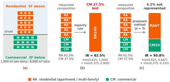
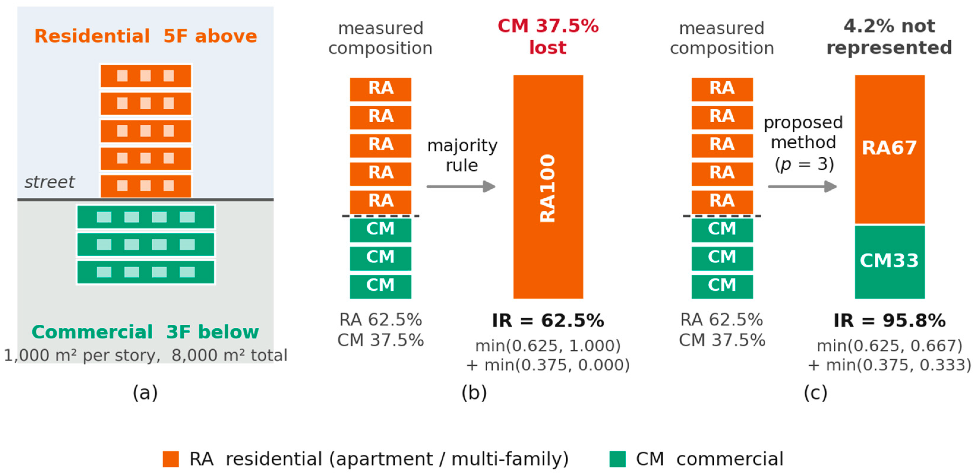
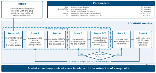
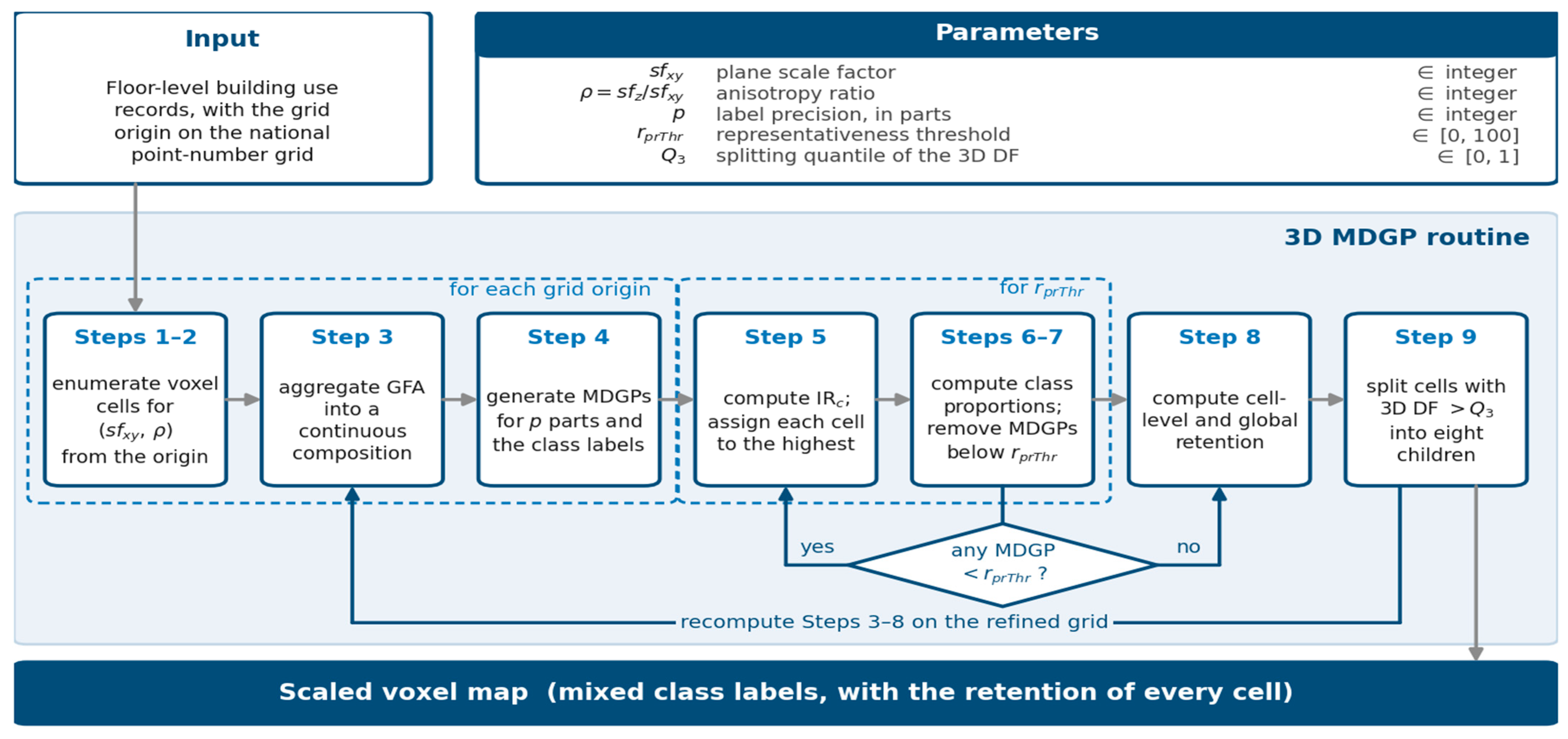
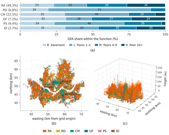
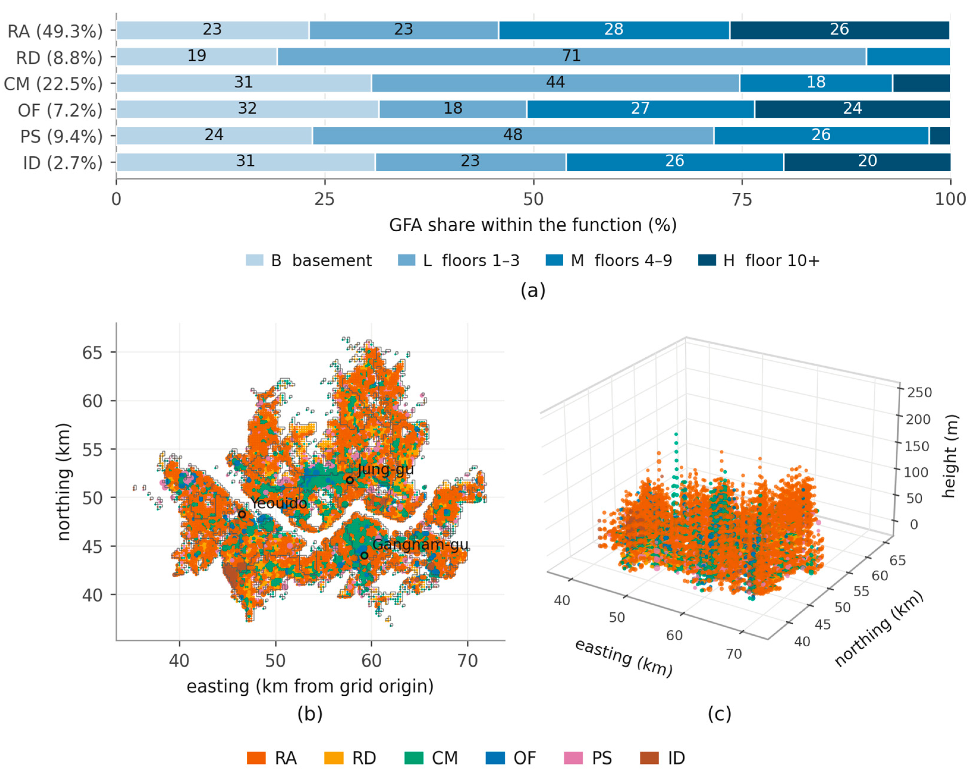
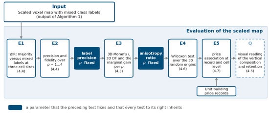
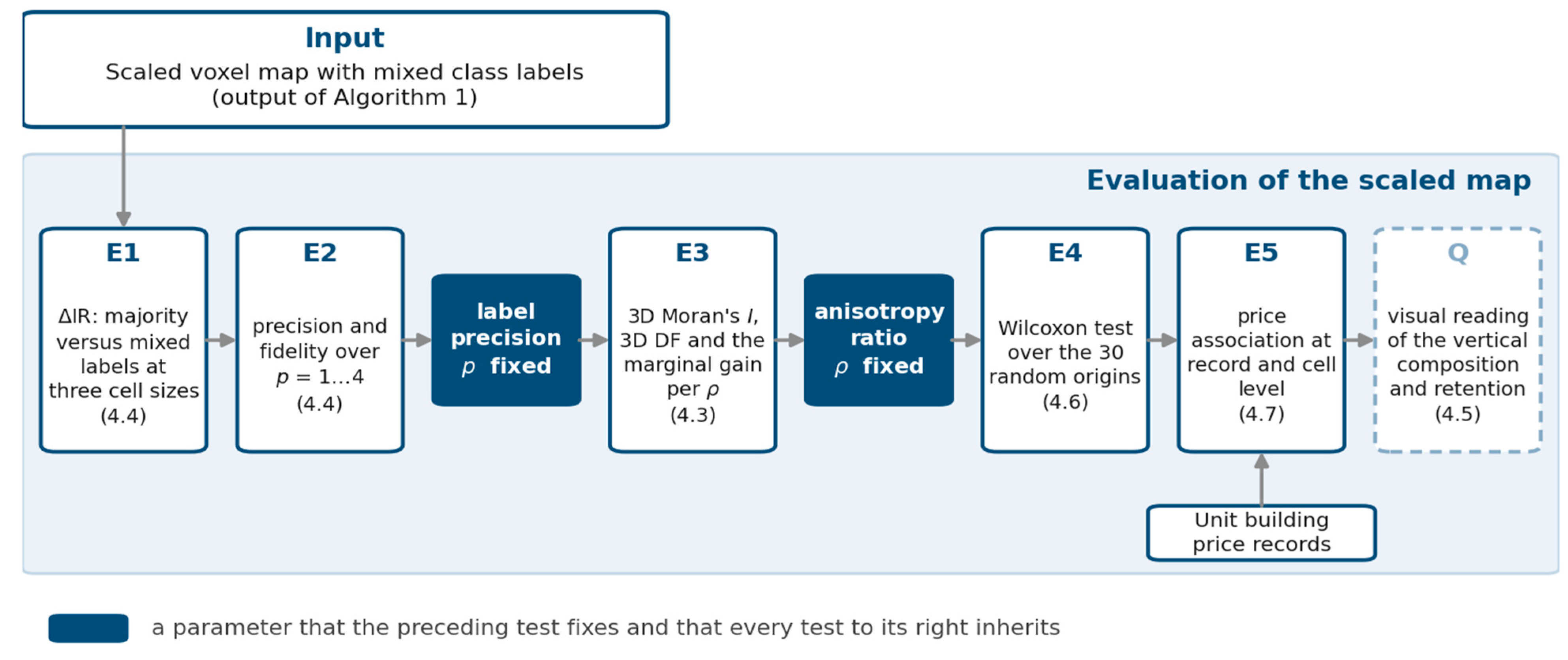
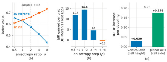
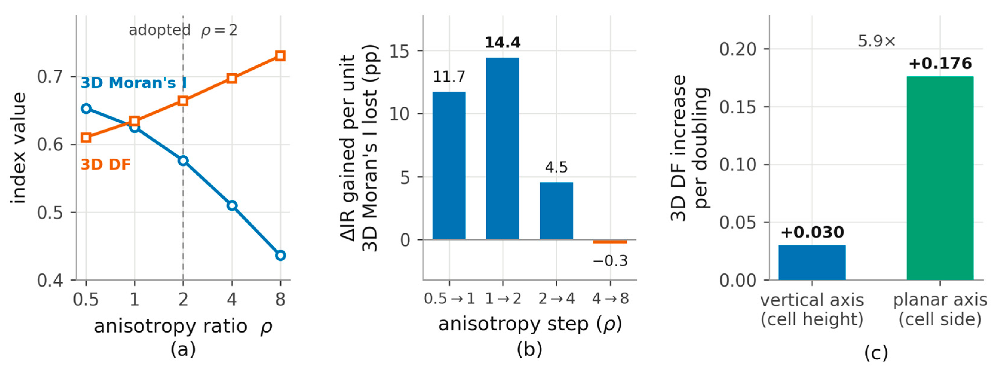
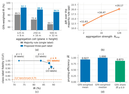
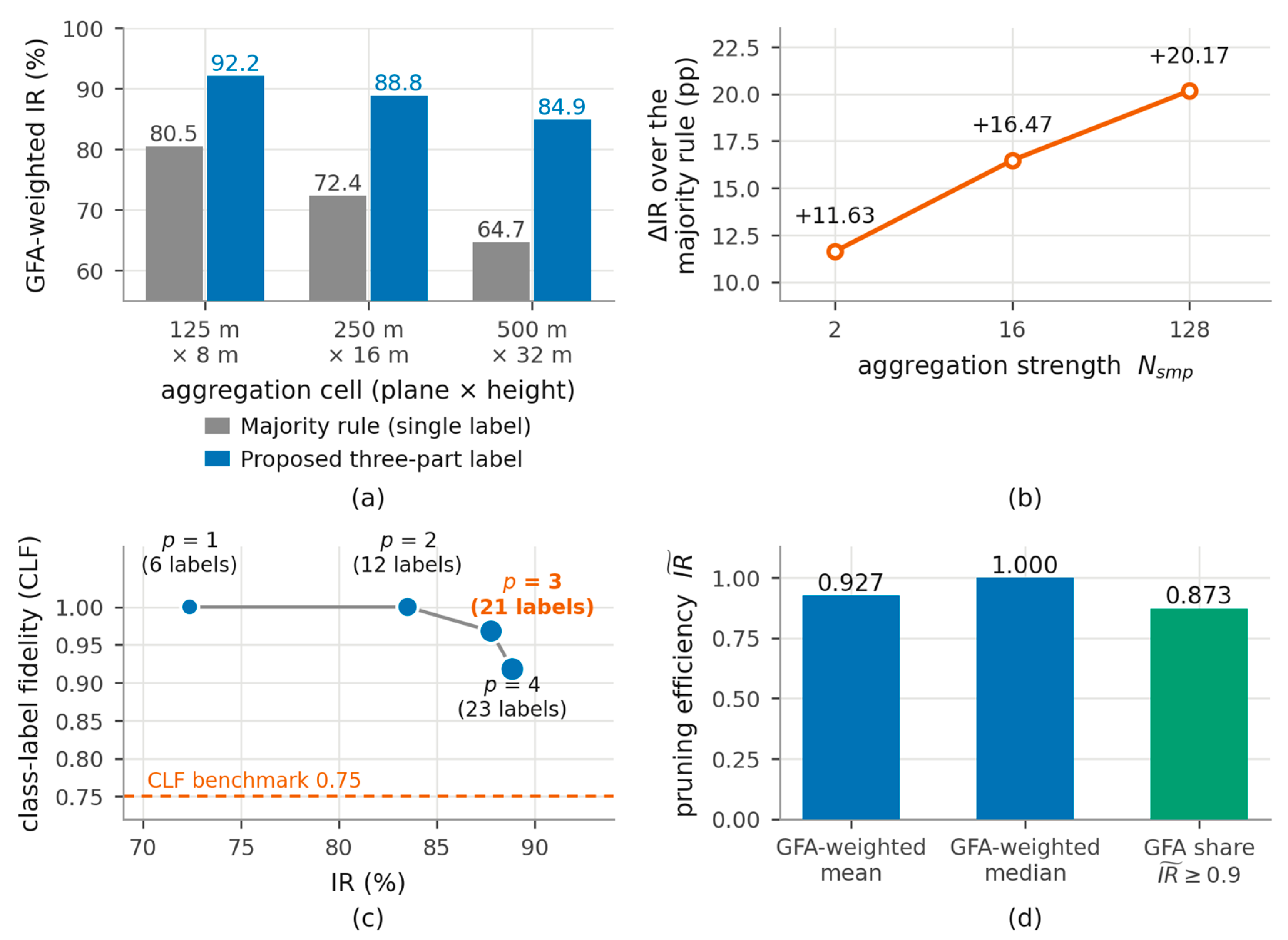
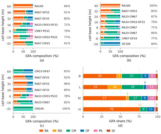
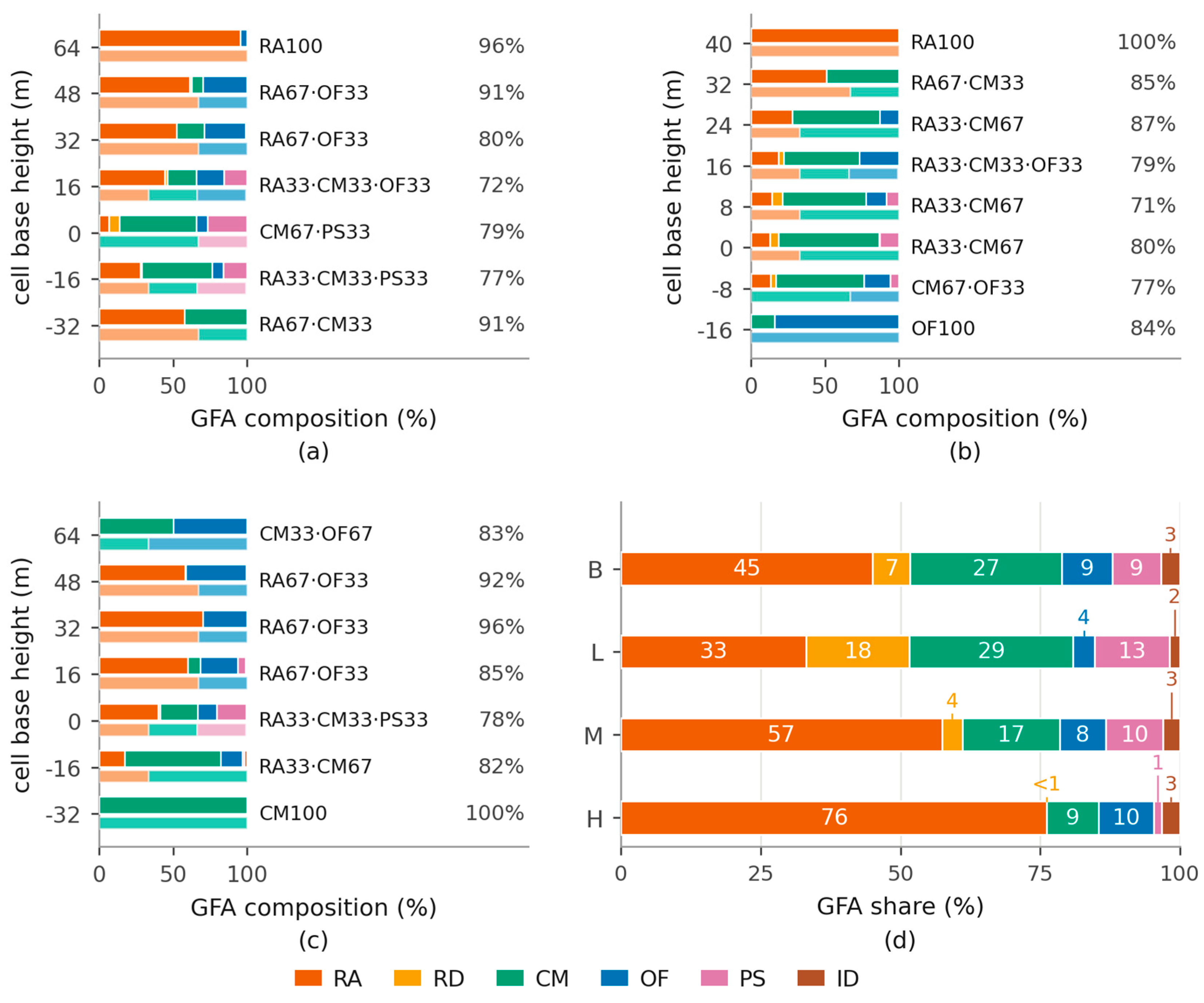
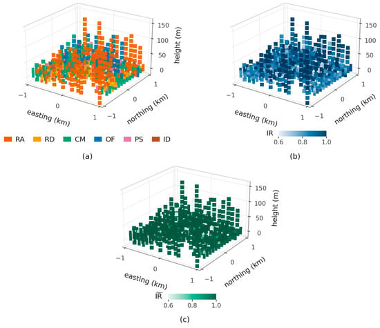
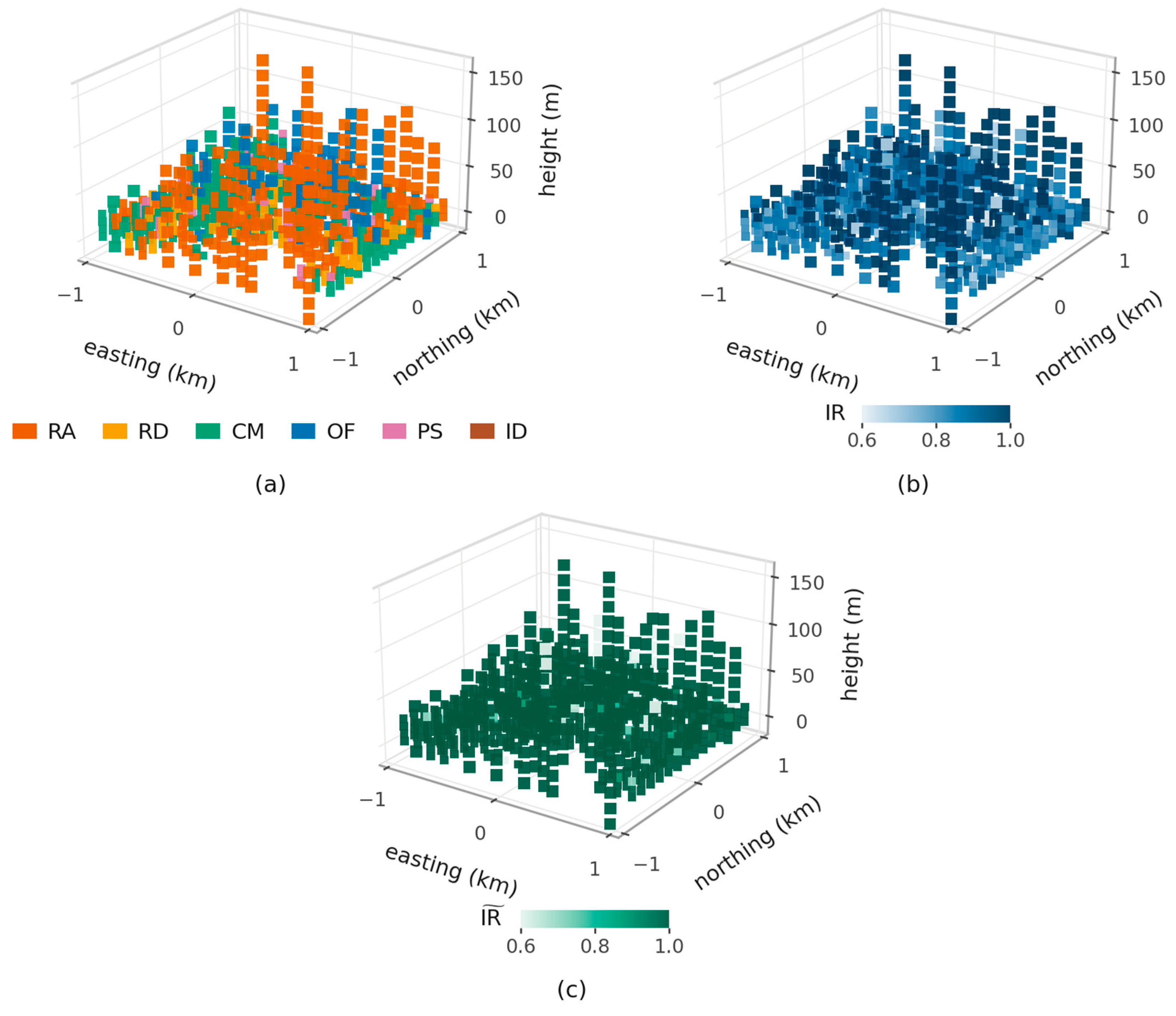
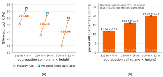
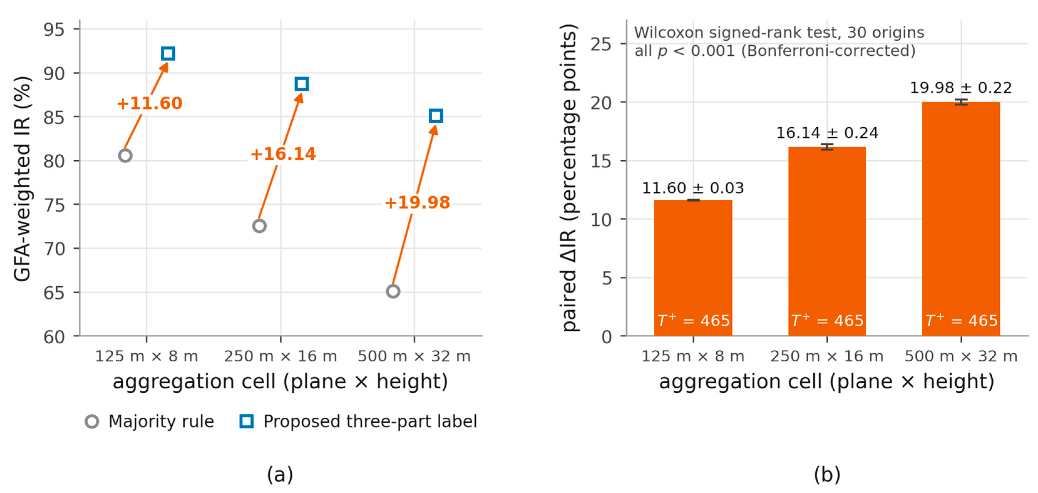
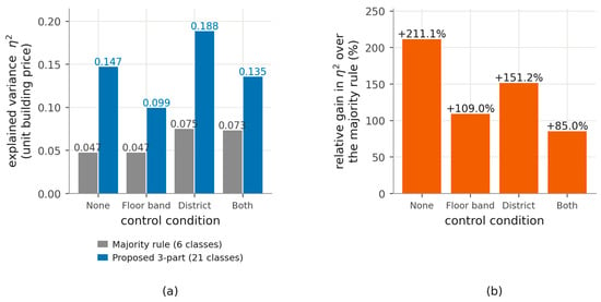
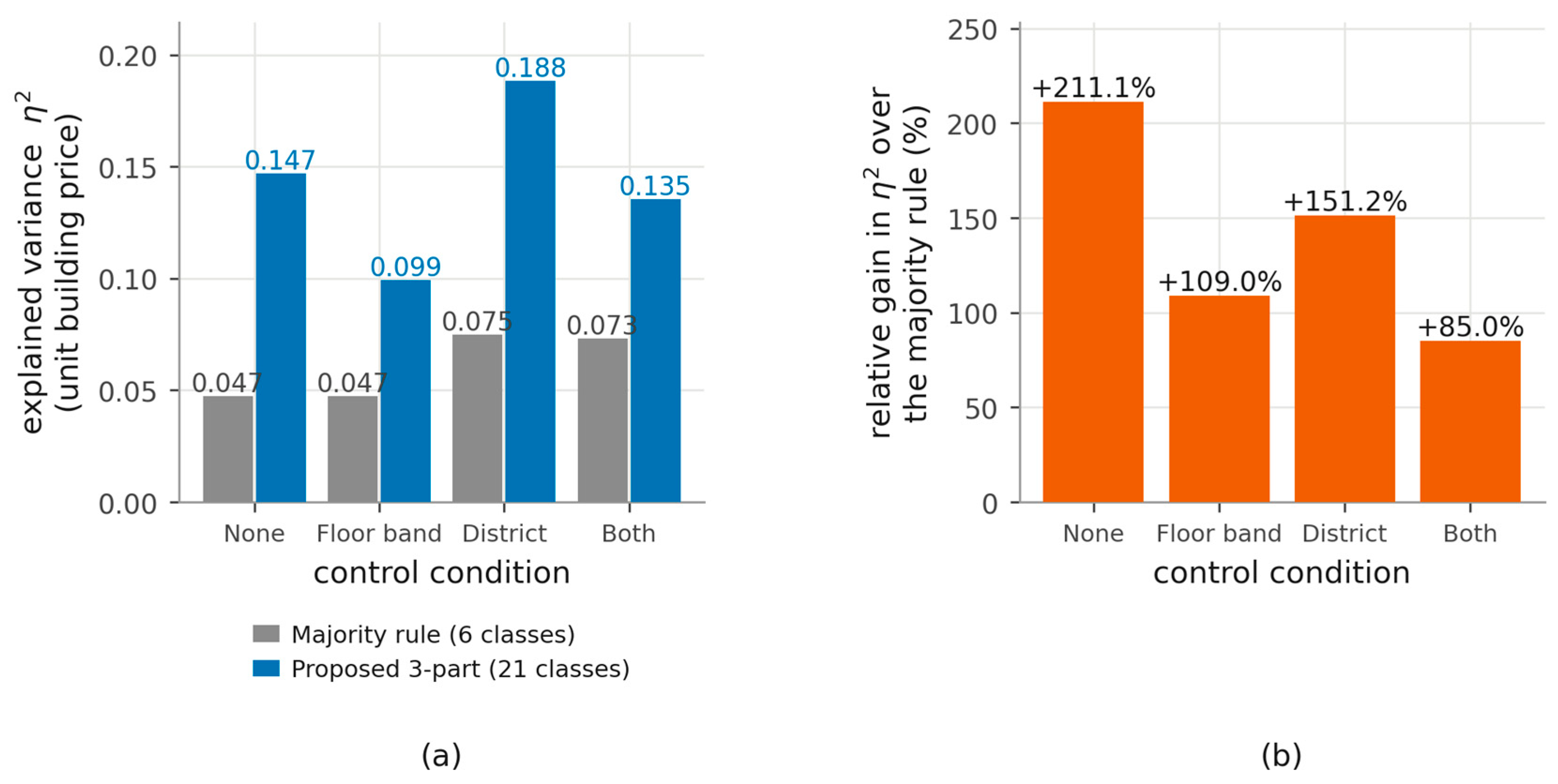

Disclaimer/Publisher’s Note: The statements, opinions and data contained in all publications are solely those of the individual author(s) and contributor(s) and not of MDPI and/or the editor(s). MDPI and/or the editor(s) disclaim responsibility for any injury to people or property resulting from any ideas, methods, instructions or products referred to in the content. |
© 2026 by the authors. Published by MDPI on behalf of the International Society for Photogrammetry and Remote Sensing. Licensee MDPI, Basel, Switzerland. This article is an open access article distributed under the terms and conditions of the Creative Commons Attribution (CC BY) license.