Low-Cost Deep Learning for Building Detection with Application to Informal Urban Planning

Abstract

This article studies the application of deep neural networks for automatic building detection in aerial RGB images. Special focus is put on accuracy robustness in both well-structured and poorly planned urban scenarios, which pose significant challenges due to occlusions, irregular building layouts, and limited contextual cues. The applied methodology considers several CNNs using only RBG images as input, and both validation and transfer capabilities are studied. U-Net-based models achieve the highest single-model accuracy, with an Intersection over Union ($IoU$) of 0.9101. A soft-voting ensemble of the best U-Net models further increases performance, reaching a best ensemble $IoU$ of 0.9665, improving over state-of-the-art building detection methods on standard benchmarks. The approach demonstrates strong generalization using only RGB imagery, supporting scalable, low-cost applications in urban planning and geospatial analysis.

1. Introduction

Cartographic information is a key resource for assisting decision-makers in urban city planning, promoting citizen welfare, and effective resource management [1]. Obtaining high-resolution remote sensing images has become easier and more cost-effective with advancements in satellite and unmanned aerial vehicle (UAV) technologies. Cartographic information can be obtained from aerial images by applying computer vision and artificial intelligence at relatively low costs [2,3] and is crucial to monitor the evolution of regions [4,5] and new applications, such as precision agriculture [6] and population estimation [7].

Despite recent advances, automated building detection in diverse urban morphologies remains a significant challenge, leading to reduced detection accuracy, particularly in regions characterized by informal planning, heterogeneous building geometries, and cluttered backgrounds [8,9,10]. Existing segmentation models often assume regular urban layouts, limiting their effectiveness in underrepresented or poorly planned areas [11,12,13].

Significant research has been carried out on automatic building extraction. However, incomplete cue extraction, sensor data dependency, and scene complexity hinder the success of automatic building extraction and modeling [5]. Furthermore, few automatic models have been developed or evaluated for scenarios with poor or nonexistent urban planning, such as those found in Latin American urbanization. Nowadays, popular methods to address automatic building detection are based on deep artificial neural networks (DNNs) that allow learning representations of data samples with several levels of abstraction [14,15], overcoming the main challenges of automatic building detection.

This article focuses on automatic building detection from remote sensing images using RGB-only aerial imagery, applied to locations with both good and poor urban planning. A particular emphasis is placed on generalization across heterogeneous urban conditions. The proposed approach is evaluated on diverse benchmark datasets, including a new manually annotated dataset from San José de las Matas (SJM), Dominican Republic, with irregular planning, to assess transfer learning performance. Three DNNs are evaluated: fully convolutional neural network (FCN), residual neural network (ResNet), and U-Net convolutional neural network. Moreover, ensembles of these deep learning models are studied. The analysis considers four aerial image datasets: Massachusetts Buildings (MBD) [16], INRIA Aerial Image Labeling (IAD) [17], WHU Building [18], and Satellite dataset II East Asia [18]. In addition, a transfer learning approach is examined by evaluating the trained models in SJM.

The studied DNNs were able to learn building extraction tasks in different contexts. The U-Net architecture outperformed FCN variants. The best (highest) Intersection over Union ($IoU$) value by U-Net models was 0.9101, improving over FCN (0.9064). Better results were achieved by training models with larger image cutouts and applying soft-voting ensembling. These competitive results were achieved using RGB-based images, without relying on more complex data. U-Net also outperformed three state-of-the-art automatic methods for building detection in a comparative analysis.

Overall, this article contributes with a robust methodology for building detection using DNNs. The studied methods have been developed to be useful in good and poor urban-planned locations and evaluated in real case studies in Latin America. This article extends a previous conference paper in which the authors explored initial approaches for automatic building extraction from urban aerial images [19]. The current work significantly expands upon it by incorporating new datasets, improved architectures, and ensemble methods. New scientific contents include (i) three new datasets included in the analysis: MBD, WHU and EAII; (ii) a new dataset generated for a poorly planned urban area in San José de las Matas, to evaluate the transfer learning capabilities of the proposed approach; (iii) model calibration and ensemble processes; and (iv) a comparison with state-of-the-art methods from the related literature.

The main contributions of this article are as follows:

• The evaluation of deep learning models (U-Net, ResNet, FCN) for building detection across diverse urban morphologies, using only RGB imagery.
• The introduction and use of SJM, a new annotated dataset of a low-planning urban area, to assess transferability.
• The proposal of a soft-voting ensemble method, improving over state-of-the-art results, with an $IoU$ up to 0.9665.

Four research questions are posed:

• RQ1: How can U-Net-based architectures be optimized and tuned to generalize across heterogeneous urban contexts while maintaining high detection accuracy?
• RQ2: To what extent RGB-only input datasets suffice in building detection, traditionally reliant on multi-modal or higher-dimensional data sources (infrared, laser)?
• RQ3: Can pre-trained models adapt to the unique characteristics of underrepresented regions with poor urban planning, without additional data annotations?

The article is organized as follows: The next section describes the problem and reviews relevant related works. Section 2.2 introduces the studied DNN architectures and methodology. Section 4 presents the data, auxiliary methods, and hyperparameters. The experimental evaluation is reported in Section 5. Finally, Section 6 presents the conclusions and the main lines for future work.

2. Problem Definition and Literature Review

This section describes the addressed problem and reviews relevant related works.

2.1. The Automatic Building Detection Problem

The growing availability of high-resolution aerial and satellite imagery has broadened remote sensing applications, particularly in urban mapping and infrastructure monitoring. A key task is automatic building extraction, which aims to identify built structures at the pixel level, generating binary segmentation masks aligned with the resolution of the input image. This is typically framed as a semantic segmentation problem, where models produce a probability map indicating the likelihood of each pixel belonging to a building. A threshold (often 0.5) converts this map into a binary mask [3,20].

This task remains challenging due to visual similarities between buildings and nearby objects, such as tanks, vegetation, or water bodies—especially in informal or low-density areas. While multispectral or hyperspectral imagery can provide enhanced discriminative features through additional spectral bands, processing such data requires significantly higher computational and storage resources, limiting its use in many practical scenarios.

Recent advances in deep learning, particularly convolutional neural networks (CNNs), have transformed the field. Unlike traditional learning approaches based on handcrafted features (e.g., texture or edge descriptors), CNNs automatically learn hierarchical representations from raw image data leading to improved generalization across varied urban settings. CNNs have yielded state-of-the-art results, especially over large annotated datasets.

2.2. Related Work

DNNs have the ability to learn features describing buildings and map them onto output layers that represent the probability that a given pixel in an image belongs to a building. The learning methods employed by DNNs have improved their efficacy and accuracy using parallel computing. Different annotated aerial high-resolution image datasets have been collected, contributing to the continuous improvement of the accuracy and quality of the results because the training process may use more data.

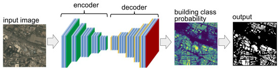
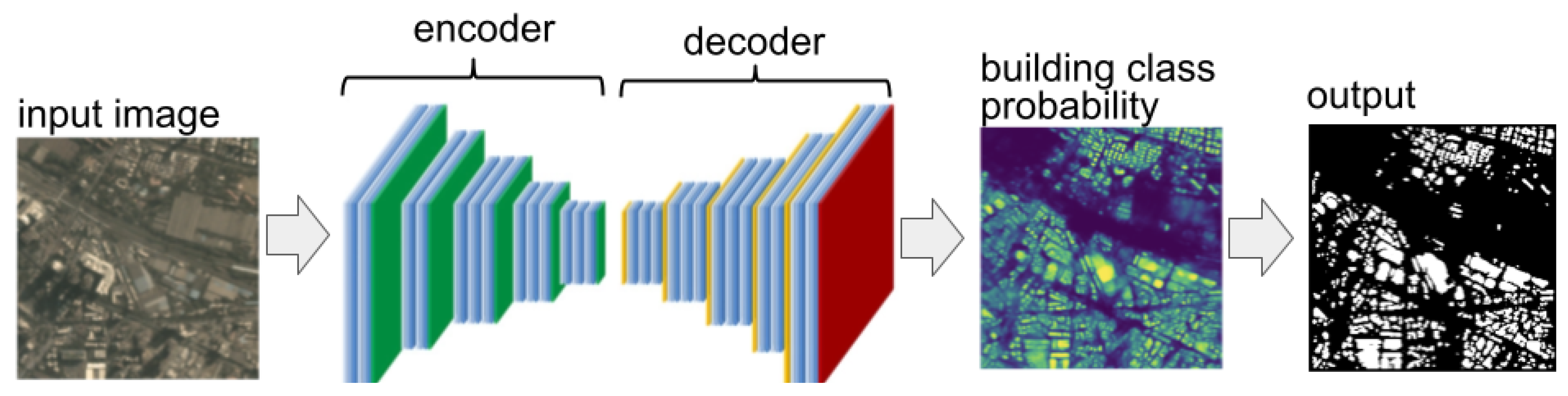
Variations of CNNs are usually applied in the building extraction literature. Figure 1 illustrates the workflow of how a CNN is applied to automatic building extraction. The white pixels in the output indicate that the corresponding pixel in the input image belongs to a building. A representative set of deep CNNs are FCNs, DeepLab, Pyramid Scene Parsing Network, LinkNet, ResNets, ResNetXt, and U-Net [21].

Figure 1. CNN architecture with encoder and decoder applied to automatic building extraction.

U-Net-based DNNs have been the most promising models for building detection. Comparative studies evaluated U-Net against LinkNet on building extraction over the Planet dataset, which covers different areas of Russia [22,23]. The evaluation considered the Sorensen–Dice coefficient (DSC) and concluded that U-Net (DSC = 0.77) was better than LinkNet (DSC = 0.72). U-Net was also applied over the SpaceNet dataset [24], including encoders to accept two separate inputs from the same geographical area: an RGB image and an infrared image. The proposed approach with $IoU$ = 0.67 improved the results provided by the original U-Net for the regions studied. The same approach (using two separate U-Net encoders) was used over the IAD dataset considering multiple loss functions.

A general issue in building detection is that buildings can be located close to each other and be merged into one single object after segmentation. A variation of U-Net proposed to deal with this problem used two encoders for detecting the buildings and for detecting the separation between buildings. The approach was able to extract the buildings and detect their boundaries. The $IoU$ results ranged from 0.60 to 0.80. Li et al. [25] studied five U-Net variations for building detection, focusing on accuracy and computational efficiency. This model variations obtained F1-score values from 0.54 to 0.89. Pan et al. [26] studied U-Net over several types of imagery databases, for example, a combination of aerial imagery with data from geographic information systems (GISs) ($IoU$ from 0.86 to 0.93), a high-resolution imagery dataset by Ahmed et al. [27] ($IoU$ from 0.43 to 0.94), and an ultra-high-resolution imagery dataset captured by UAVs.

Singla and Ramani [28] evaluated standard U-Nets, a U-Net with ResNet-34 backbone, and a U-Net with VGG-19 for building detection on WorldView datasets. A method was proposed based on GIS data from Open Street Map for obtaining datasets. The U-Net with ResNet-34 backbone provided the best $IoU$ results ranging from 0.84 to 0.89. Xu et al. [29] combined U-Net and ResNet for building extraction on multispectral imagery from Vaihingen (2500 × 2500 px, spatial resolution of 9 cm and 16 frames labeled at the pixel level) and Potsdam (orthorectified infrared–RGB images of 6000 × 6000 px, spatial resolution of 5 cm, and 24 samples labeled at the pixel level). The approach was compared with remote sensing, FCN, and CNN + Random Forest. U-Net–ResNet obtained better accuracy and F1 score (from 0.88 to 0.95), improving over the other methods. Robinson et al. [30] applied U-Net with a ResNet-34 encoder for building detection with a minimal quantity of labeled data on high-resolution satellite images (0.5 m/px). The model was trained over images from Jordan with few sparse polygon annotations. The recall on unseen building footprints was 0.87, and the R² in building count in 200 × 200 m areas was 0.93.

Jiwani et al. [31] applied a DeepLabV3+ architecture with a Dilated ResNet backbone for building footprint detection on RGB satellite images. The training included an F-Beta measure to address class imbalance and a weighted boundary loss to enhance separation of adjacent buildings, and a cross-dataset training strategy was used to improve model robustness. A recall of 0.92 and a precision of 0.93 were obtained on the SpaceNet dataset. Gizzini et al. [32] studied five Class Activation Mapping (CAM) explainability methods for semantic building footprint detection. A novel evaluation methodology and an entropy-based metric were introduced to assess model uncertainty and explainability in detection tasks. Seg-Score-CAM computed the best results over the WHU dataset, particularly in highlighting pixels relevant to boundaries and minimizing model uncertainty.

Li et al. [20] developed a framework for generating precise vectorized maps for geospatial applications from very high resolution aerial imagery. The framework combined semantic detection (U-Net), bounding box detection (Cascade R-CNN), and key point detection (Cascade CNN), integrating the outputs through Delaunay triangulation to generate accurate building polygons. The best $IoU$ was 0.851.

Gonzalez et al. [33] proposed a method to automatically identify building typologies relevant to seismic risk assessment using CNNs applied to images from Google Street View. The model achieved high precision and recall in classifying the materials and lateral load-resisting systems of buildings in Medellín, Colombia. Recent advancements in transformer-based architectures have shown competitive performance compared to CNN-based methods. For instance, STransU2Net integrates Swin Transformer Blocks (STBs) within skip connections to enhance global context understanding and local feature extraction, achieving an $IoU$ of 0.91 on the Aerial Imagery dataset [34]. CTANet combines ConvNeXt as an encoder with a Bilateral Hybrid Attention Transformer (BHAT) decoder, capturing both texture edges and background features, achieving $IoU$ values of 0.76 on MBD, 0.92 on WHU, and 0.83 on IAD [35]. These transformer-based models surpass CNNs in accuracy, but their higher computational demands may limit their applicability. In contrast, CNN-based approaches offer a balance between efficiency and accuracy, making them more practical for real-world scenarios.

The main contributions of the research in this article over the previous approaches are as follows:

• This study expands on the use of U-Net architectures for building detection by introducing and benchmarking hybrid U-Net–ResNet and U-Net–ResNeXt models across multiple standard datasets, showcasing their robustness and versatility.
• Exhaustive parameter tuning is performed on the proposed models to achieve the best possible results for building detection.
• An ensemble approach is proposed to address challenges like closely spaced buildings, providing effective solutions without adding computational complexity, unlike methods using dual encoders from the literature.
• Only RGB imagery is used, enhancing the applicability of the models in real-world scenarios where specialized data (infrared imagery, GIS datasets) may not be available.
• The analyzed models demonstrate strong generalization by applying pre-trained architectures on global datasets to diverse scenarios, including the underrepresented San José de las Matas dataset, overcoming the limitations of sparse-label approaches.

3. Methodology

This section describes the studied DNN architectures for building detection and the methodology applied for development and evaluation.

3.1. DNNs Considered in the Study

Residual neural networks: DNNs have been proven to properly learn increasingly complex functions but suffer from the vanishing gradient problem (weights are not updated and no learning is performed [21]). ResNet was developed to mitigate the gradient vanishing problem in dense CNNs by introducing skip connections among residual units to bypass one or more layers. Several variants of ResNet have been proposed, e.g., ResNet34, ResNet50, and ResNet101. The number in the name indicates the number of layers. These CNNs have one MaxPool layer at the beginning, one AveragePool layer at the end, and convolution layers. ResNeXt [36] applies the “split–transform–merge” paradigm to replace the standard residual blocks in ResNet. The block input is projected onto a set of lower-dimensional representations (channels) to which convolutional filters are applied separately to merge the results. In ResNeXt, all the convolution paths have the same topology. The number of paths is a hyperparameter itself, called cardinality (C).

Fully convolutional neural networks: FCNs were proposed to keep the locality in learning, required to deal with image segmentation (i.e., labeling individually each pixel of the input image) [37]. FCNs replace fully connected output layers with 1 × 1 convolutional layers. After performing the CNN downsampling operations to the input image, the 1 × 1 convolutional layers upsample to calculate the pixelwise output (label map). Thus, the classification output and the input image have a one-to-one correspondence at the pixel level: the channel dimension at any output pixel holds the classification results for the input pixel at the same spatial position.

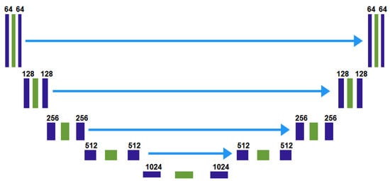
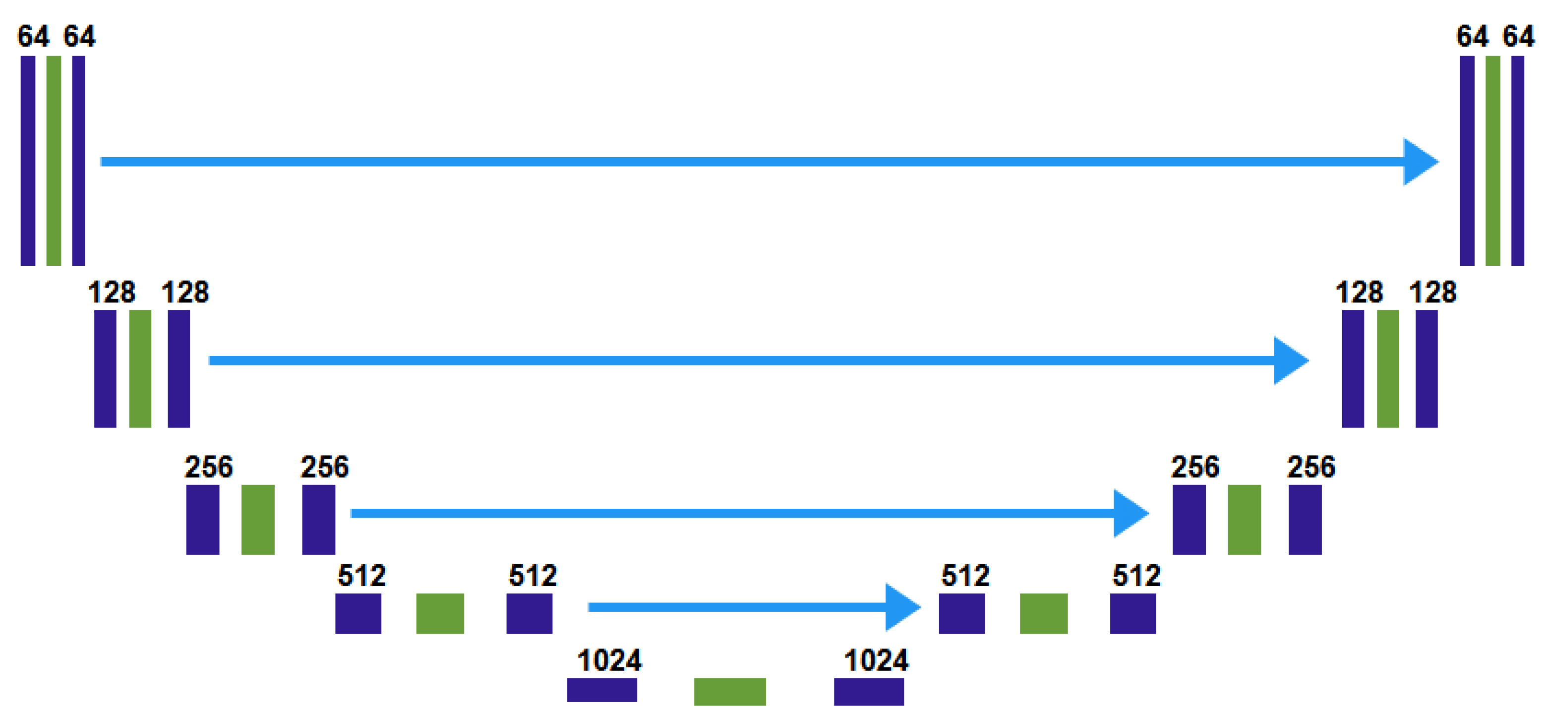
U-Net: The U-Net architecture (Figure 2) has a contraction path (encoder) and an expansive path (decoder). Symmetry on paths yields a U-shaped architecture.

Figure 2. U-Net architecture (example for a 32 × 32 input).

The main goal of the contraction path is to reduce the spatial dimensions of images and capture relevant information. A series of convolution layers (represented in blue in Figure 2) and pooling layers (represented in green) are used to capture relevant features. Five blocks are used: (i) applies two 3 × 3 convolution layers followed by a ReLU layer, the number of channels is increased to 64, and a 2 × 2 max pool layer (stride 2) is applied; (ii) applies two 3 × 3 convolution layers followed by a ReLU layer, the number of channels is doubled to 128, and a 2 × 2 max pool layer is applied; (iii) and (iv) repeat the procedures in the previous blocks, doubling the number of channels; (v) the number of feature channels is doubled again to 1024, and a 3 × 3 convolution layer followed by a ReLU layer is applied.

The expansive path is aimed at upsampling the extracted feature map to generate a useful segmentation map for the input image. Five blocks are used: (v) applies a 3 × 3 convolution layers followed by a ReLU layer and a 2 × 2 up-convolution layer to upsample the spatial dimensions and reduce the number of channels to 512; (iv), (iii), and (ii) apply skip connections, two 3 × 3 convolution layers followed by a ReLU layer, and a 2 × 2 up-convolution layer to reduce the number of channels to 256; (i) applies two 3 × 3 convolution layers followed by a ReLU layer, a 1 × 1 convolution layer, and an activation layer to reduce the number of channels to match the number of classes.

The main benefits of U-Net over other DNNs are due to its simple structure (using convolutional, ReLU activation, and max pooling layers) and it exhibits very competitive results in segmentation by requiring few training data (i.e., labeled images).

3.2. Problem Instances

This section describes the datasets considered for training and evaluation of the proposed DNNs for automatic building extraction from urban aerial images.

3.2.1. Massachusetts Buildings Dataset (MBD)

The dataset consists of 151 aerial images in Boston (USA), each one of 1500 × 1500 px covering an area of 2.25 km². The entire dataset covers 340 km². The data are randomly divided into a training set of 137 images, a test set of 10 images, and a validation set of 4 images. MBD mainly covers urban and suburban areas and buildings of various sizes, including single houses and garages. The annotated images have the three RGB channels, with values of (255, 0, 0) for the Building class and (0, 0, 0) for the No Building class.

3.2.2. INRIA Aerial Image Labeling Dataset (IAD)

The dataset includes color aerial imagery covering a total area of 810 km², divided into 405 km² for the training set and 405 km² for the testing set. The data cover different regions in the USA and Austria, representing different types of urban areas, from small cities to megacities [17]. The semantic segmentation of images considers two different labels: Building and No Building. Including data (images) from several types of cities allows IAD to evaluate the generalization capabilities of the segmentation algorithms. Thus, the training and test sets do not overlap, i.e., they include images from different cities.

The training dataset has 180 color images of 5000 × 5000 px, each one covering an area of 1500 × 1500 m in Austin, Chicago, Kitsap County, West Tyrol, and Vienna. The test dataset has 180 images with the same features, in Bellingham, Bloomington, Innsbruck, San Francisco, and East Tyrol.

3.2.3. WHU Building Dataset–Christchurch (WHU)

The dataset has over 187,000 individual buildings extracted from aerial images with a spatial resolution of 0.3 over Christchurch, New Zealand. WHU includes 8188 images of size 512 × 512 px. The training set has 4736 (130,500 buildings), the validation set has 1036 (14,500 buildings), and the test set has 2416 (42,000 buildings). The annotated images are single-channel with a value of 255 for the Building class and 0 for the No Building class.

3.2.4. Satellite Dataset II East Asia (EAII)

The dataset consists of six contiguous satellite images covering 550 km² in East Asia with a ground resolution of 2.7 m. Each image is divided into 17,388 mosaics of 512 × 512 px, divided in training (21,556 buildings) and test (7529 buildings) sets. Originally, both training and test sets were divided between images with and without buildings. In this article, only those with at least one positive case in the image were considered. Thus, the training set was reduced to 3135 images and the test set to 903.

Of the presented datasets, WHU has the most rural areas, but the non-built-up territories depicted are mostly covered with trees and green grass of a very similar tone and regular terrain. EAII has much greater variety: from roads and plantations that turn vegetated territory into irregular shapes, to arid and dark appearances seemingly caused by the conditions and quality in which the images were taken, and not only by the elements that make up the terrain. Although many images of residential buildings make up the EAII dataset, many buildings have an irregular distribution, following winding roads or being in isolated areas not seen in any of the previous datasets, so it is estimated that urban planning for EAII is much less than for the previous cases.

3.2.5. San José de las Matas (SJM)

The dataset was created in this research to evaluate building detection models in a city where urban planning was probably absent for its development. San Jose de las Matas is a municipality located in the province of Santiago, Dominican Republic, covering an area of 3.41 km², which is divided into 640 × 640 pxs images. The dataset was generated through satellite images from Google Maps, and annotations were manually generated using the Labelbox tool [38], which allows the drawing of segments on the original images.

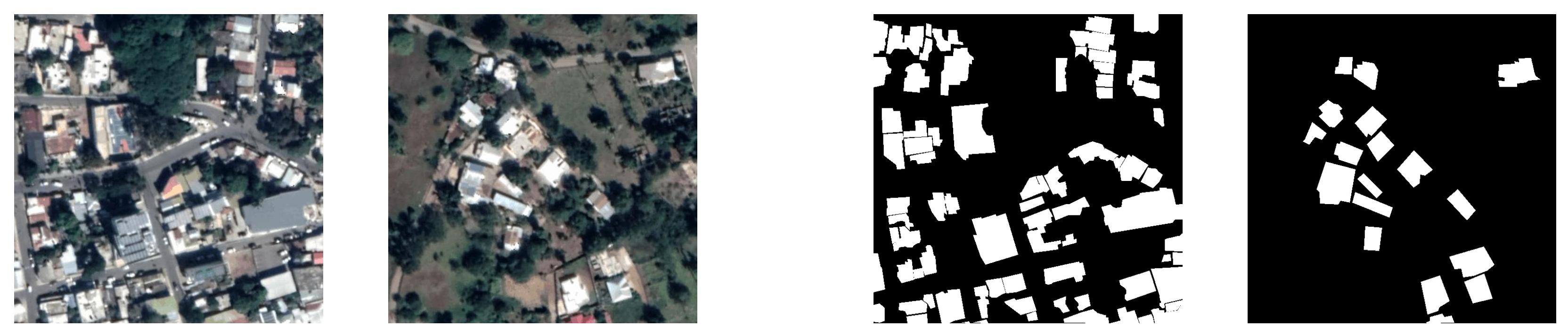
San Jose de las Matas has mainly low-rise residential buildings arranged in different orientations to each other, which contrasts with images in MBD and IAD datasets, where in many cases, the walls of the buildings are aligned (either perpendicular or parallel) with the surrounding streets. Another characteristic of SJM is the significant presence of trees, whose canopies usually exceed the height of the buildings, altering the appearance of their rectangular roofs from a satellite perspective (an example is presented in Figure 3).

Figure 3. Original images from SJM dataset (left) and groud truth for the original images (right).

3.3. Methodological Stages

An iterative development and evaluation methodology was applied. Candidate models were progressively (and eliminatively) analyzed in a pipeline involving five stages, which are described next.

Stage 1, initial architecture selection: The studied DNN architectures were trained and evaluated for each dataset using a learning rate (LR) of 8 × ${10}^{-5}$ and the Dice loss function. The three models with the highest average $IoU$ for all datasets were selected for each approach.

Stage 2, resizing MBD and IAD datasets: The collected datasets have significant differences in the number of images and their quality. WHU and EAII datasets have a large number of small-sized images, whereas MBD and IAD have a much smaller quantity of images but much larger in size. The fact that IAD and MBD images are large implies that very small cuts (480 × 480 px) are generated in each training instance, compared to the original size of the image, so a lot of information would be ignored. Although the loss of information can be mitigated by increasing the number of training epochs, the plan for the later stages was to unify the datasets, so a presumably better approach was to scale the datasets images down to smaller sizes, similar to the WHU and EAII datasets. To address the problem of information loss for large dimension images, the auxiliary datasets IAD2500, IAD1250, IAD1000, MBD750, and MBD500 were generated, to keep an auxiliary dataset for each original dataset. As with the selection of architectures, the best-performing auxiliary dataset was chosen based on the average $IoU$ metric score for the models obtained in stage 1.

Stage 3, hyperparameters for models trained with the unified dataset: The models were trained with the union of the datasets resulting from stage 2 with two variations: using 100% of the images in the dataset and using only 50% to improve computational efficiency. The studied cost functions were Dice loss and a combination of cross-entropy and focal Tversky, $CEFT\left(c\right)=CE\left(c\right)+FT\left(c\right)/2$. In FTL, $\alpha =0.99$ and $\beta =0.01$ were chosen to minimize false negatives. Two values of $\gamma$ (0.25 and 0.1) were studied, $\gamma <1$ was selected because the DNNs were applied to areas with buildings, so it was expected that they would be able to learn the “easy” examples, according to the Tversky index [39]. Three values were studied for LR: 4 × ${10}^{-5}$, 8 × ${10}^{-5}$, and $1.6$ × ${10}^{-4}$. The models were also trained using the union of the datasets and not each dataset separately, to improve their generalization capability and the overall results. However, the union of the datasets resulted in a large number of images (13,301), demanding more training time. To study whether the models were capable of achieving good results with fewer data (and less training time), they were also trained with 50% of the total data and the results were compared. The hyperparameters used to train the candidate models were CEFT with $\gamma =0.25$ (CEFT_0.25) and $\gamma =0.10$ (CEFT_0.1) and dataset proportions of 100 and 50.

Stage 4, models calibration: The three models with the best results in the previous stage were selected for each approach. Then, all models were calibrated using the temperature scaling mechanism.

Stage 5, models voting: Voting was applied over the best models: the class of each pixel was decided based on the classification of each model. The voting considered the three models with the best $IoU$ (the minimum number of models necessary) to validate whether that method yielded better results than those obtained by each model individually. Two types of voting were analyzed: hard vote and soft vote. In all cases, votes from all models were weighted the same.

3.4. Approaches

Two approaches were applied in each stage of the proposed methodology:

• Validation: At each step, the $IoU$ resulting from each model was measured with the test set of the dataset that the model was trained on.
• Transfer: At each step, the $IoU$ resulting from each model was measured with the SJM dataset. In each stage, the models were trained with the IAD, WHU, MBD, and EAII datasets, but the $IoU$ taken into account for selecting the best model was the one obtained when evaluating over the SJM dataset.

4. Experimental Setup

This section describes the DNN architectures analyzed, the evaluation metrics, the hardware platform used to run the experiments, and the software libraries for development.

4.1. Evaluated DNNs Architectures

The experimental analysis studied several DNN architectures to find the best one for the building detection problem. An initial list of candidate architectures was determined to perform the experiments. These architectures were defined by combining the architectures introduced in Section 3.1. The studied architectures were (i) FCN-8, an FCN with a VGG-16 as the backbone (i.e., encoder) [37]; (ii) FCN-ResNet50, an FCN with a ResNet50 as the backbone; (iii) FCN-ResNet101, an FCN with a ResNet101 as the backbone; (iv) U-Net-ResNet34, a U-Net with a ResNet34 as the backbone; (v) U-Net-ResNet50, a U-Net with a ResNet50 as the backbone; (vi) U-Net-ResNet101, a U-Net with a ResNet101 as the backbone; and (vii) U-Net-ResNeXt50, a U-Net with a ResNeXt50 as the backbone.

4.2. Data Augmentation

Data augmentation methods were applied to obtain additional data for model training. Two approaches were taken: (1) generate new files that build a new set from an original one with certain transformations (i.e., offline augmentation), and (2) apply transformations on the image during the training stage (i.e., online augmentation).

Offline augmentation allowed us to obtain sets with smaller images, and in some cases with an RGB-to-BGR channel transformation. The size reduction not only aimed at generating a larger dataset, but for the case of IAD, there was also a limitation due to the image size (5000 × 5000). Experiments revealed that a maximum cut (approximately) of 2016 × 2016 was needed to not run out of memory and to avoid losing significant information. For WHU and EAII, no data were generated as they were sufficiently represented with the original samples. The sets resulting from applying offline augmentation were (i) IAD2500, 2500 × 2500 tiles of original IAD images and RGB to BGR inversion; (ii) IAD1250, 1250 × 1250 tiles of original IAD images and RGB to BGR inversion; (iii) IAD1000, 1000 × 1000 tiles of original IAD images; (iv) MBD750, 750 × 750 tiles of original MBD images; and (v) MBD500, 500 × 500 tiles of original MBD images.

Two online transformations were applied to each training image: a random crop of size 480 × 480; and with a probability of 75%, apply a horizontal inversion, vertical inversion, or random 90° rotation transformation. Full experimental details are provided in the project report [40].

4.3. Performance Metric

The metric used to evaluate the proposed models was the $IoU$, a standard metric used for comparing the similarity between two arbitrary shapes. Given an input image, the $IoU$ provides a measure of the similarity between the predicted region and the input image (ground truth). The $IoU$ is largely preferred in the literature over other metrics, mainly because of its robustness to class imbalance, in a problem where the number of background pixels or regions without buildings often significantly outweighs the number of building pixels.

The $IoU$ is defined as the size of the intersection divided by the size of the union of the two regions (Equation (1), where X is the actual class mapping of an image, given by the ground truth, and Y is the map predicted by the DNN).

$$IoU={\displaystyle \frac{|X\cap Y|}{|X\cup Y|}}$$

(1)

4.4. Calibration Methods

The estimated calibration error ($ECE$) was used to empirically measure the calibration of models. The $ECE$ measures the difference between expected accuracy and expected confidence, resulting in a scalar value. It is calculated as the weighted average of the difference between accuracy and confidence of the intervals (Equation (2), where n is the total number of samples in all bins). Perfect calibration is achieved when $ECE=0$.

$$ECE=\sum _{m=1}^M{\displaystyle \frac{B_m}{n}}|acc\left(B_m\right)-conf\left(B_m\right)|$$

(2)

Temperature scaling [41] was used for calibration. This method takes a model that extends a previous one, to correct the calibration error. The calibrated model is generated after the original model is fully trained. Temperature scaling is applicable to classification tasks for K classes by rescaling the logit vector $z_i$ as expressed by ${\widehat{q}}_i={max}_k\sigma (z_i^k/T)$, where $z_i^k$ is the logit of data element i for class k, T is the temperature parameter to be adjusted, and $\sigma$ is the softmax function. T is trained with a loss function on verification data.

4.5. Development and Execution Platform

The approaches were developed in Python 3.10 using PyTorch 1.9 and the segmentation models library. OpenCV 4.5.1 and Albumentation 1.0.2 were used for image manipulation and data augmentation. Experiments were performed on the high-performance-computing infrastructure of the National Supercomputing Center, Uruguay [42].

5. Experimental Evaluation and Discussion

This section reports and discusses the results of the DNN approaches applied to building extraction.

5.1. Stage 1: Selection of the Best Architectures

Table 1 reports the $IoU$ values for each architecture, dataset, and evaluation approach. The three best average $IoU$ values are marked in bold to identify the selected architectures.

Table 1. $IoU$ values for each architecture, combining validation and transfer approaches.

Architecture	Validation					Transfer
	IAD	MBD	WHU	EAII	Average	IAD	MBD	WHU	EAII	Average
FCN-8	0.8386	0.7803	0.9572	0.9450	0.8803	0.8342	0.8293	0.8161	0.8709	0.8376
FCN+ResNet50	0.8965	0.8172	0.9700	0.9629	0.9117	0.8706	0.8128	0.8445	0.8655	0.8484
FCN+ResNet101	0.8848	0.8130	0.9685	0.9624	0.9072	0.8704	0.8398	0.8297	0.8891	0.8573
U-Net+ResNet34	0.8715	0.8267	0.9692	0.9619	0.9073	0.8738	0.8185	0.8390	0.8846	0.8540
U-Net+ResNet50	0.8780	0.8097	0.9693	0.9615	0.9046	0.7727	0.8255	0.8553	0.8865	0.8350
U-Net+ResNet101	0.9177	0.8279	0.9690	0.9597	0.9186	0.8781	0.8188	0.8270	0.8869	0.8527
U-Net+ResNeXt50	0.8965	0.8147	0.9720	0.9612	0.9111	0.8805	0.8281	0.8212	0.8733	0.8508

Results in Table 1 indicate that all models produced similar results except for FCN-8. The three architectures that produced the highest $IoU$ values for validation were FCN+ResNet50, U-Net+ResNet101, and U-Net+ResNeXt50, and for transfer, they were FCN+ResNet101, U-Net+ResNet34, and U-Net+ResNet101. Thus, U-Net+ResNet101 provided highly competitive results for both validation and transfer.

5.2. Stage 2: Resizing MBD and IAD Datasets

Table 2 reports the $IoU$ results for architecture, approach, and resized dataset. In IAD, the highest $IoU$ for validation was obtained when training with IAD2500. For transfer, the most competitive results were achieved by IAD and IAD1000 (with a slight $IoU$ difference, lower than 0.01). IAD1000 was selected to train the models because the online image transformation (to 480 × 480 images) applied during the training would have a worse impact on the results for IAD, which has the largest image size (5000 × 5000 px images). Focusing on MBD, the best $IoU$ was achieved on MBD500 for validation. For transfer, the best results were obtained when using MBD. Based on the results, two datasets for training the models were defined by combining IAD2500, WHU, MBD500, and EAII for validation, and IAD1000, WHU, MBD, and EAII for transfer. These two datasets had a high number of images, which led to a significant computational cost during the training process.

Table 2. $IoU$ values for each auxiliary dataset and approach in stage 2. The best average $IoU$ values are marked in bold.

Validation
Dataset	Architecture				Dataset	Architecture
	FCN+ ResNet50	U-Net+ ResNet101	U-Net+ ResNeXt50	Average		FCN+ ResNet50	U-Net+ ResNet101	U-Net+ ResNeXt50	Average
IAD1000	0.8469	0.8802	0.8694	0.8694	MBD500	0.8185	0.8232	0.8274	0.8230
IAD1250	0.8666	0.8611	0.8771	0.8683	MBD750	0.8100	0.8145	0.8235	0.8160
IAD2500	0.9181	0.9057	0.9102	0.9113	MBD	0.8172	0.8279	0.8147	0.8199
IAD	0.8965	0.9177	0.8965	0.9036
Transfer
Dataset	Architecture				Dataset	Architecture
	FCN+ ResNet50	U-Net+ ResNet101	U-Net+ ResNeXt50	Average		FCN+ ResNet50	U-Net+ ResNet101	U-Net+ ResNeXt50	Average
IAD1000	0.8782	0.8441	0.8757	0.8660	MBD500	0.8116	0.8056	0.8051	0.8074
IAD1250	0.8071	0.8374	0.7861	0.8102	MBD750	0.8272	0.7354	0.7877	0.7834
IAD2500	0.8571	0.8207	0.8443	0.8407	MBD	0.8398	0.8185	0.8270	0.8284
IAD	0.8704	0.8738	0.8781	0.8741

5.3. Stage 3: Hyperparameters for Models Trained with the Unified Dataset

The reported hyperparameter configuration results consider the architectures selected in previous stages, the cost function and LR values presented in Section 2.2, and the created datasets with 100% and 50% of images.

5.3.1. Validation

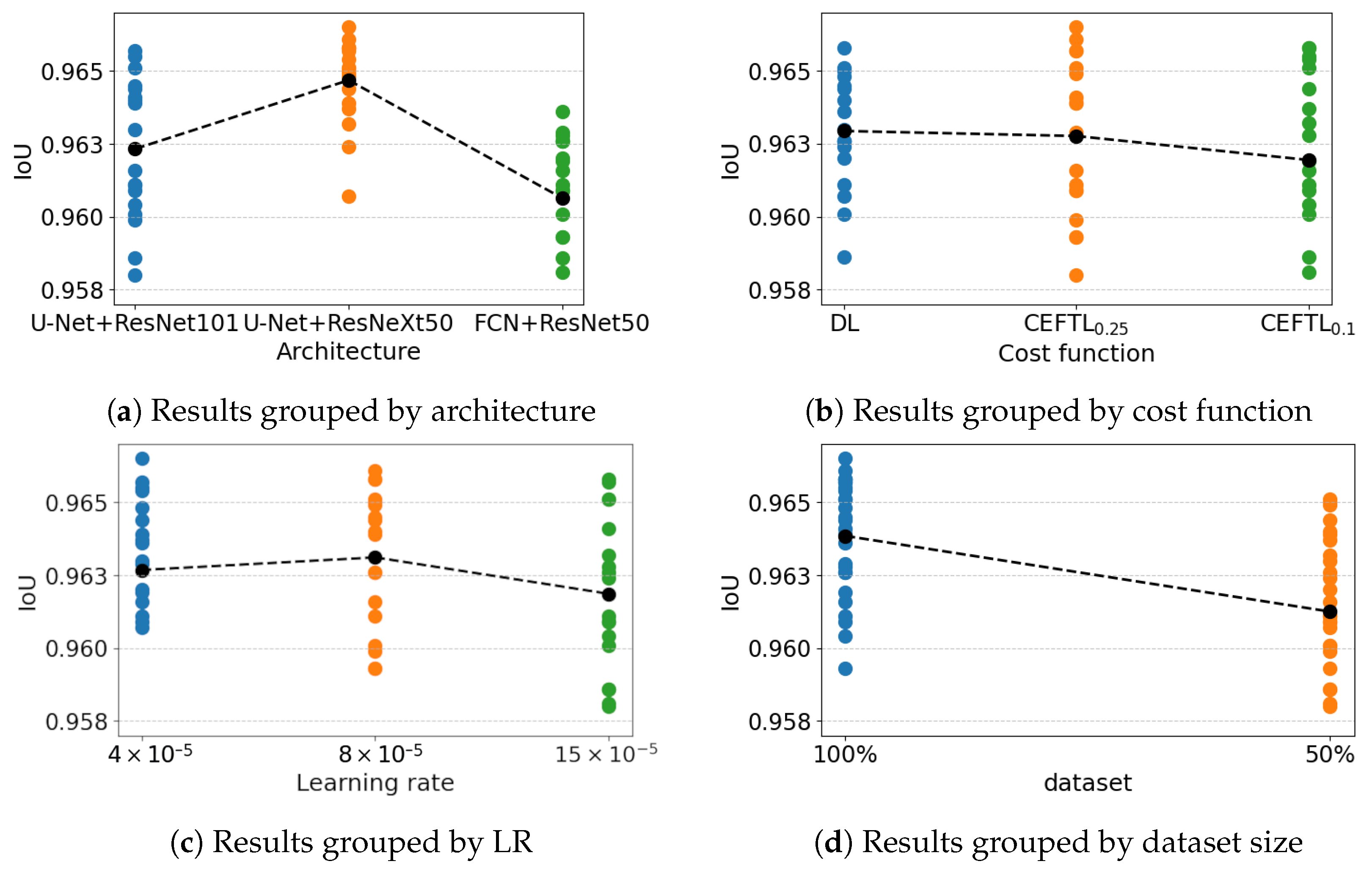
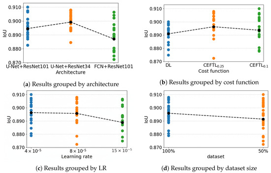
Figure 4 shows the distribution of results grouped by each studied hyperparameter (architecture, cost function, LR, and dataset size). The outline solution with a value of 0.9506 is excluded to better represent the overall distributions. U-Net+ResNeXt50 computed the highest $IoU$ ($0.9665$) and average $IoU$ ($0.9646$) values (Figure 4a). In contrast, the architecture using FCN as an encoder showed the lowest $IoU$ (average $IoU$ = $0.9607$).

Figure 4. $IoU$ values for hyperparameter configuration experiments for validation, grouped by each configuration parameter.

The highest $IoU$ was achieved using CEFT_0.25. The average $IoU$ value for Dice, CEFT_0.25, and CEFT_0.1 were $0.9629$, $0.9628$, and $0.9619$, respectively. According to these results, no considerable variations in $IoU$ results for the evaluated cost functions were shown. Regarding LR, the best $IoU$ was obtained with the 4 × ${10}^{-5}$ rate. Figure 4c illustrates that the least competitive results were achieved by the highest LR value evaluated in these experiments. The best average $IoU$ value ($0.9633$) was obtained by using LR 8 × ${10}^{-5}$.

Models trained with the full dataset obtained the best $IoU$ results, with an average $IoU$ of $0.9639$, over the dataset with 50% of images ($0.9028$). Obtaining better $IoU$ from models that train with more data was expected because more data allow the models to avoid overfitting problems. Considering the computational time, training with the full dataset took 66% longer than training with 50% of images, which represents a significant computational cost reduction when reducing the dataset size.

5.3.2. Transfer

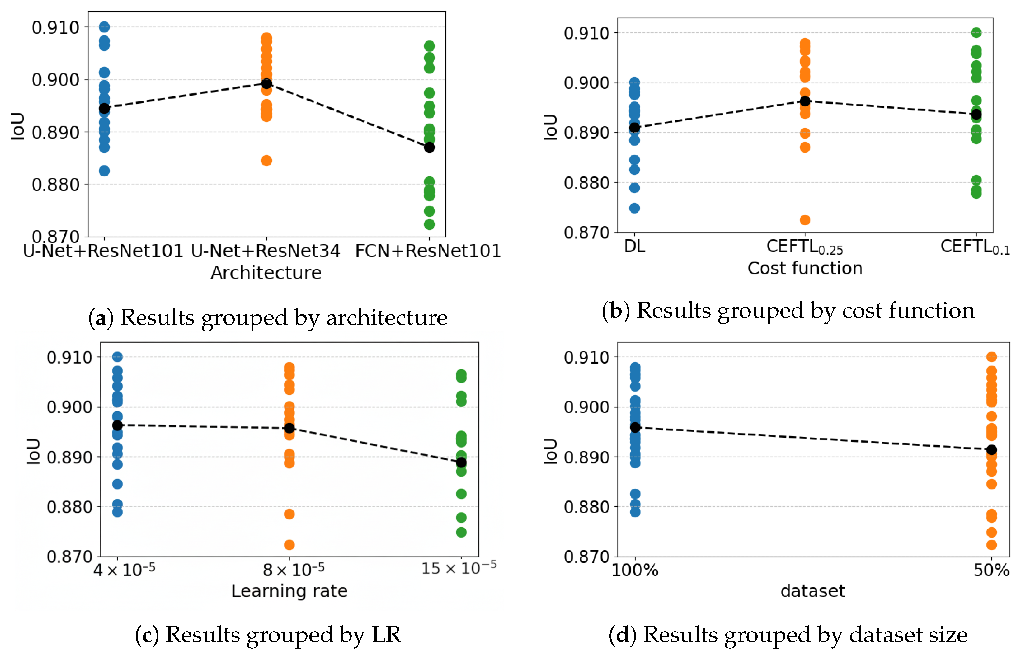
Figure 5 shows the distribution of results grouped by the each studied hyperparameter.

Figure 5. $IoU$ values in hyperparameter configuration experiments for transfer. Each plot shows the results grouped by each configuration parameter.

The best average $IoU$ results were achieved by U-Net+ResNet architectures (Figure 5a). U-Net+ResNet34 obtained the highest average $IoU$ ($0.8992$). In contrast, the architecture that used FCN as an encoder showed the least competitive results (average $IoU$ of $0.8871$). Although there appeared to be a difference between the results of the models with U-Net and FCN as encoders (Figure 5a), the difference between their $IoU$ average was only around one hundredth.

Better $IoU$ values were obtained when using CEFT than deep learning. In turn, the best $IoU$ was obtained with an LR of 4 × ${10}^{-5}$. The least competitive results were achieved by 15 × ${10}^{-5}$. The best average $IoU$ ($0.8958$) was obtained by using an LR of 4 × ${10}^{-5}$.

Regarding the dataset size, training the models with the entire dataset resulted in more robust models than training with only 50% of the images (Figure 5d). The $IoU$ results when using 100% of the samples were less scattered, ranging from 0.8805 to 0.9079, compared to the results when using only 50% of the images, which ranged from 0.8579 to 0.9101. The most competitive $IoU$ when training with the entire dataset was 0.9079, which was achieved by using the U-Net+ResNet34 architecture applying the CEFT_0.25 cost function and an LR of 8 × ${10}^{-5}$. The highest $IoU$ when training with 50% of the dataset was 0.9101, which was obtained by using the U-Net+ResNet101 architecture and applying the CEFT_0.1 cost function and an LR of 4 × ${10}^{-5}$.

5.3.3. Comparative Analysis: Validation vs. Transfer

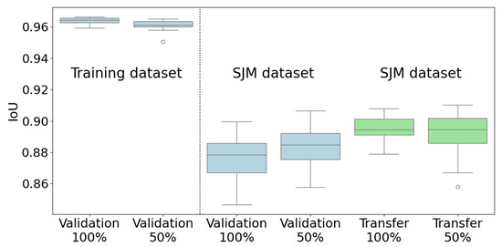
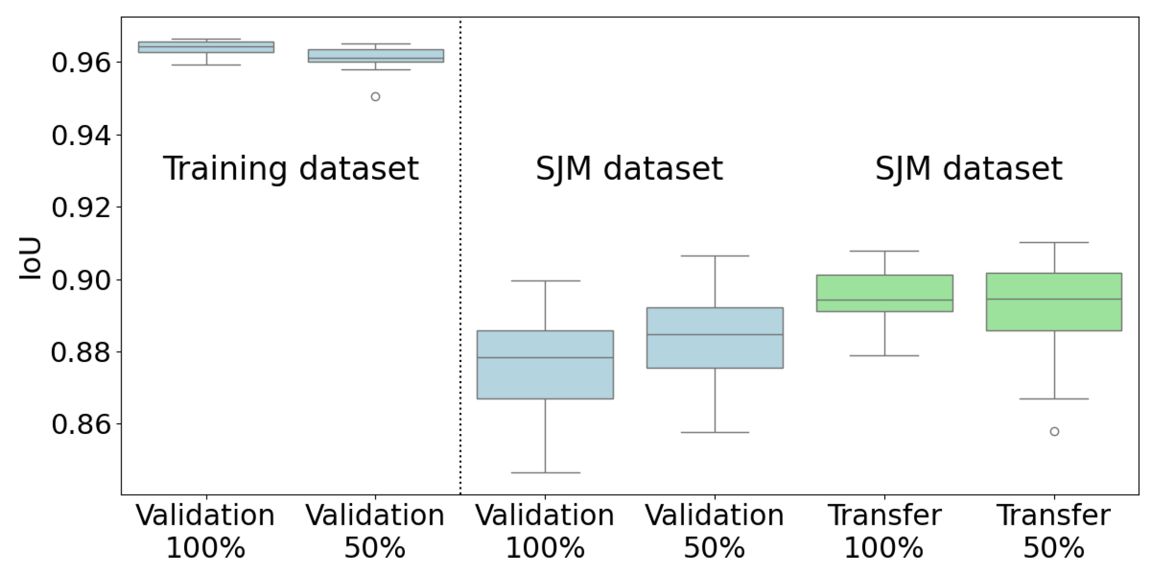
Figure 6 compares $IoU$ values between models evaluated on the SJM dataset and their validation counterparts on the training dataset. Transfer models achieved more competitive results, with higher $IoU$ values and lower dispersion than validation models. These results highlight the importance of selecting architectures suited to the target dataset.

Figure 6. Comparison of $IoU$ values obtained for validation and transfer models on their training dataset and the SJM dataset.

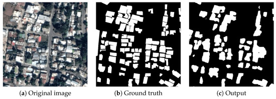
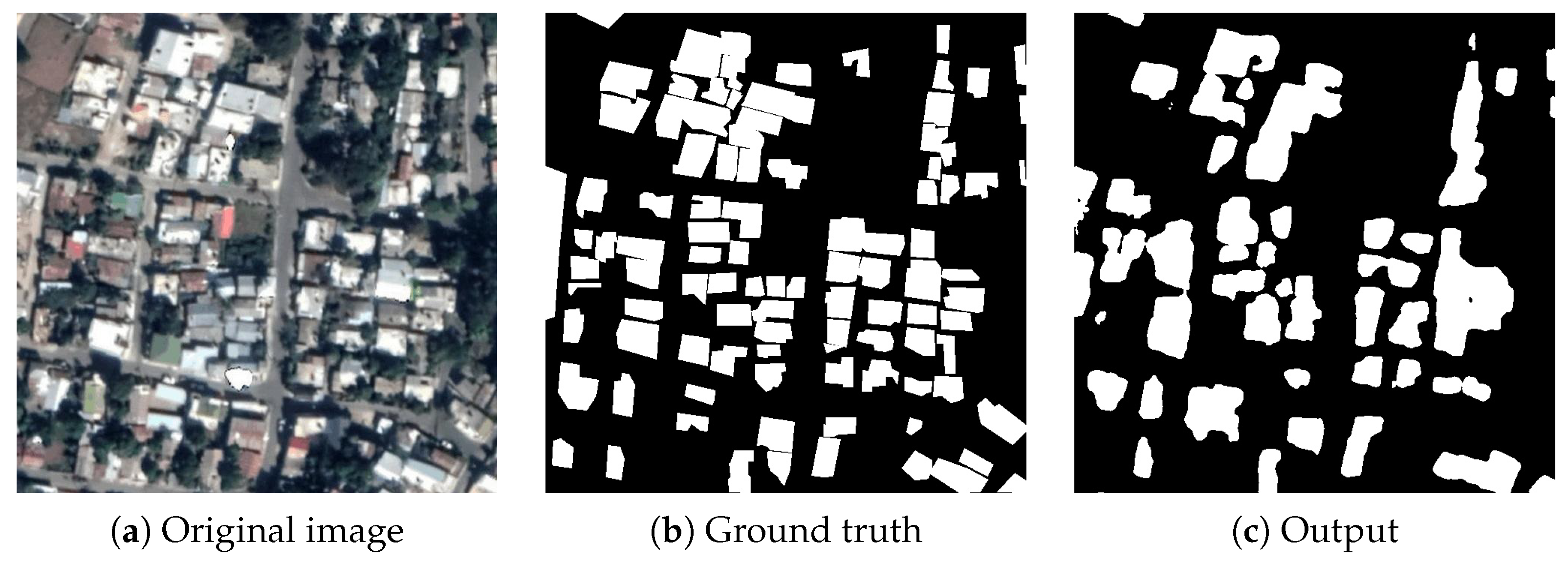
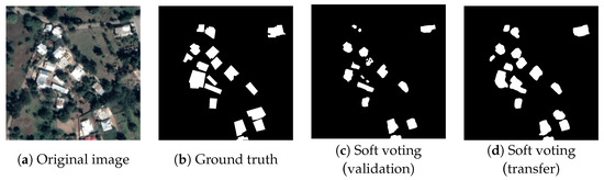
Regarding validation models, the $IoU$ results on the training dataset were significantly better than on the SJM dataset. Results worsened when using 50% of the images. However, the results on the SJM dataset improved when training on fewer images, which might be because the models generalized better (i.e., models trained with the entire dataset probably suffered from overfitting). An illustrative example is the U-Net+ResNet101 architecture using the CEFT_0.25 cost function and an LR of 15 × ${10}^{-5}$. The $IoU$ results for training datasets was lower than the other models, but the $IoU$ obtained for the SJM dataset was one of the highest. Figure 7 shows an example of the original input image, the ground truth, and the output computed by this best transfer model on the SJM dataset.

Figure 7. Example of validation results on the SJM dataset.

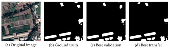
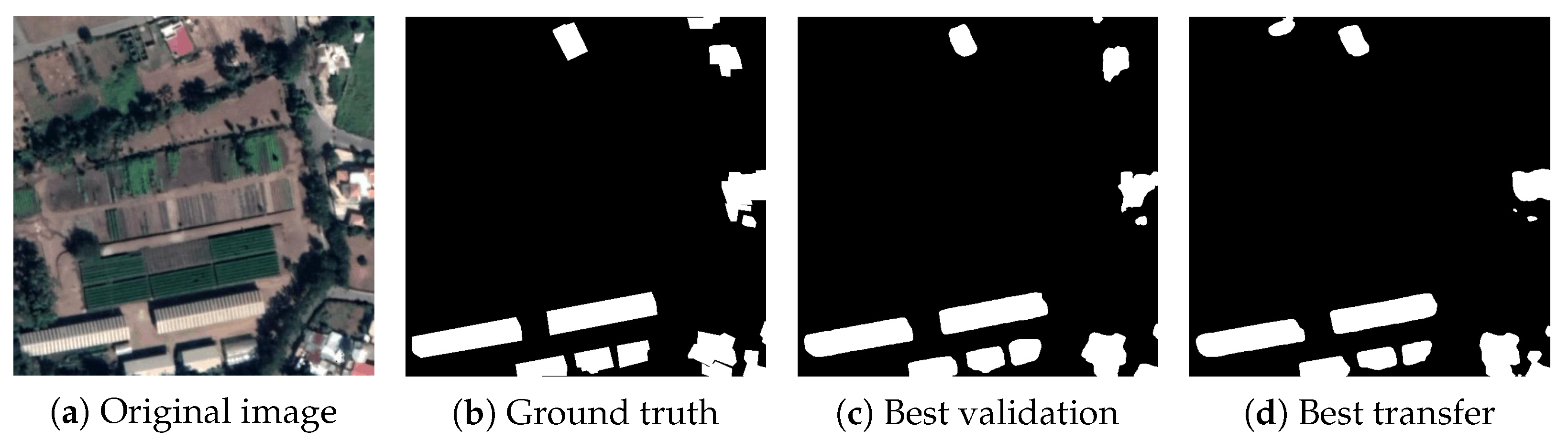
Figure 8 presents another example of an SJM input image, the ground truth, and the computed outputs with the best $IoU$ results for validation and transfer experiments.

Figure 8. Sample results of the best validation and transfer models.

The area in Figure 8 shows several constructions at the bottom, top, and right ends of the image. Both models produced good results, but with some disparities: (a) the best validation model correctly detected the buildings in the top right, and the best transfer model did not; (b) the best transfer model provided more accurate shapes of the buildings in the bottom right than the best validation model. Thus, the best way to obtain the most accurate building extraction model was to combine several models by applying voting [43]. Voting combines multiple machine learning models to create a model that returns a unique output. The ensemble of learning models applying voting improves the accuracy of each model separately. Voting strategies were studied in stage 5.

5.4. Stage 4—Models Calibration

Table 3 reports the results of the calibration of the best models from the previous stage, applying the temperature scaling method. The studied temperature values were in the interval $[1,10]$ with a step of $0.01$. For each model, the temperature $T_{min}$ that minimized $ECE$, the $IoU$ before and after applying temperature scaling, the improvement in $IoU$ (${\Delta }_{\mathrm{IoU}}$), and the percentage of improvement regarding the ideal improvement (${\Delta }^{*}$) are reported.

Table 3. $IoU$ values, before and after applying temperature scaling.

Validation
Model	Cost	LR	% Dataset	${\mathit{T}}_{min}$	$\mathit{IoU}$  pre TS	$\mathit{IoU}$  post TS	${\Delta }_{\mathrm{IoU}}$	${\Delta }^{*}$
U-Net+ResNeXt50	CEFT0.25	4 × 10−5	100%	2.842	0.9665	0.9679	0.0014	4.18%
U-Net+ResNeXt50	CEFT0.25	8 × 10−5	100%	3.150	0.9661	0.9676	0.0015	4.42%
U-Net+ResNeXt50	Dice	8 × 10−5	100%	3564	0.9658	0.9676	0.0018	5.26%
Transfer
Model	Cost	LR	% Dataset	${\mathit{T}}_{min}$	$\mathit{IoU}$  pre TS	$\mathit{IoU}$  post TS	${\Delta }_{\mathrm{IoU}}$	${\Delta }^{*}$
U-Net+ResNet101	CEFT0.1	4 × 10−5	50%	1980	0.9593	0.9604	0.0011	2.70%
U-Net+ResNet34	CEFT0.25	8 × 10−5	100%	2790	0.9557	0.9577	0.0020	4.51%
U-Net+ResNet101	CEFT0.25	8 × 10−5	100%	3564	0.9592	0.9607	0.0015	3.68%

Slight improvements were obtained after applying temperature scaling. The best improvement was 0.002 for the U-Net+ResNet34 model with the CEFT_0.25 cost function and an LR of 8 × 10⁻⁵, using the full dataset. However, when considering that the best methods had high $IoU$ values, the ideal improvement was always as low as 4.4%. The percentage of improvement considering the ideal case was between 2.70% and a maximum value of 5.26%.

All methods underestimated low probabilities, i.e., $[0.2,0.5)$, and overestimated high probabilities, i.e., $[0.6,1.0)$, before calibration. In samples where the models indicated a prediction probability of being positive of around 0.3, the actual results exceeded 0.4 in all cases. Conversely, when the models predicted a probability of being positive near of around 0.9, the outcomes were below 0.6 in all instances. After calibration, samples in the lower intervals were shifted towards higher ones, increasing the correct predictions of positive samples (confidence greater than $0.5$) and improving the final $IoU$.

Although it is expected that a calibrated model’s accuracy changes with respect to its uncalibrated version, the variation may not always be in favor of the metric and may even degrade it. For the studied problem, the computed $IoU$ values improved, were robust, and were close to the optimum values.

5.5. Stage 5—Model Voting

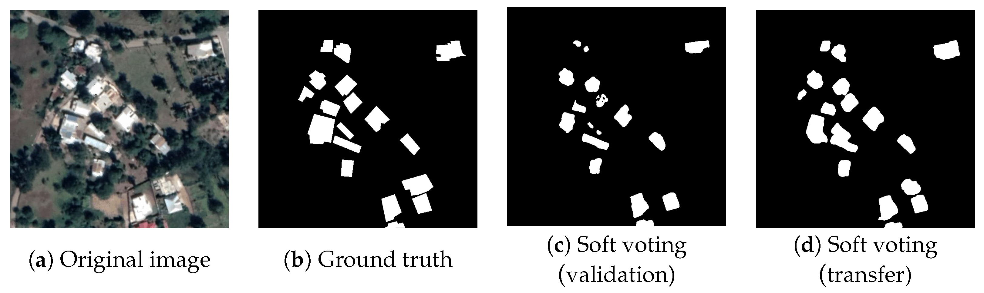
For the soft-voting model, $IoU$ results were 0.8850 for validation and 0.9163 for transfer. The hard-voting model yielded $IoU$ results of 0.8774 for validation and 0.9089 for transfer. Soft voting computed slightly better results than hard voting, and the transfer approach improved over the standard validation approach.

Mixed results were obtained in the comparison between model voting and individual models. For the validation approach, soft voting was better than individual $IoU$ for models U-Net+ResNeXt50 with the CEFT_0.25 cost function and an LR of 4 × 10⁻⁵ and for U-Net+ResNeXt50 with the Dice cost function and an LR of 8 × 10⁻⁵ but did not improve over U-Net+ResNet50 with the CEFT_0.25 cost function and an LR of 8 × 10⁻⁵ model. For the transfer approach, the soft-voting model improved over the individual results of all studied models. Hard voting improved over the studied models, except for U-Net+ResNet101 with the CEFT_0.1 cost function and an LR of 4 × 10⁻⁵. Figure 9 shows an example of soft-voting outcome for both approaches.

Figure 9. Soft voting results for validation and transfer approaches on the SJM dataset.

5.6. Examples of Building Detection

This subsection presents representative examples of building detection results for a set of six images belonging to the SJM dataset with different characteristics, from residential areas with closely spaced houses to rural areas or with other types of constructions.

5.6.1. Validation

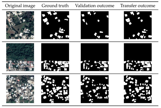
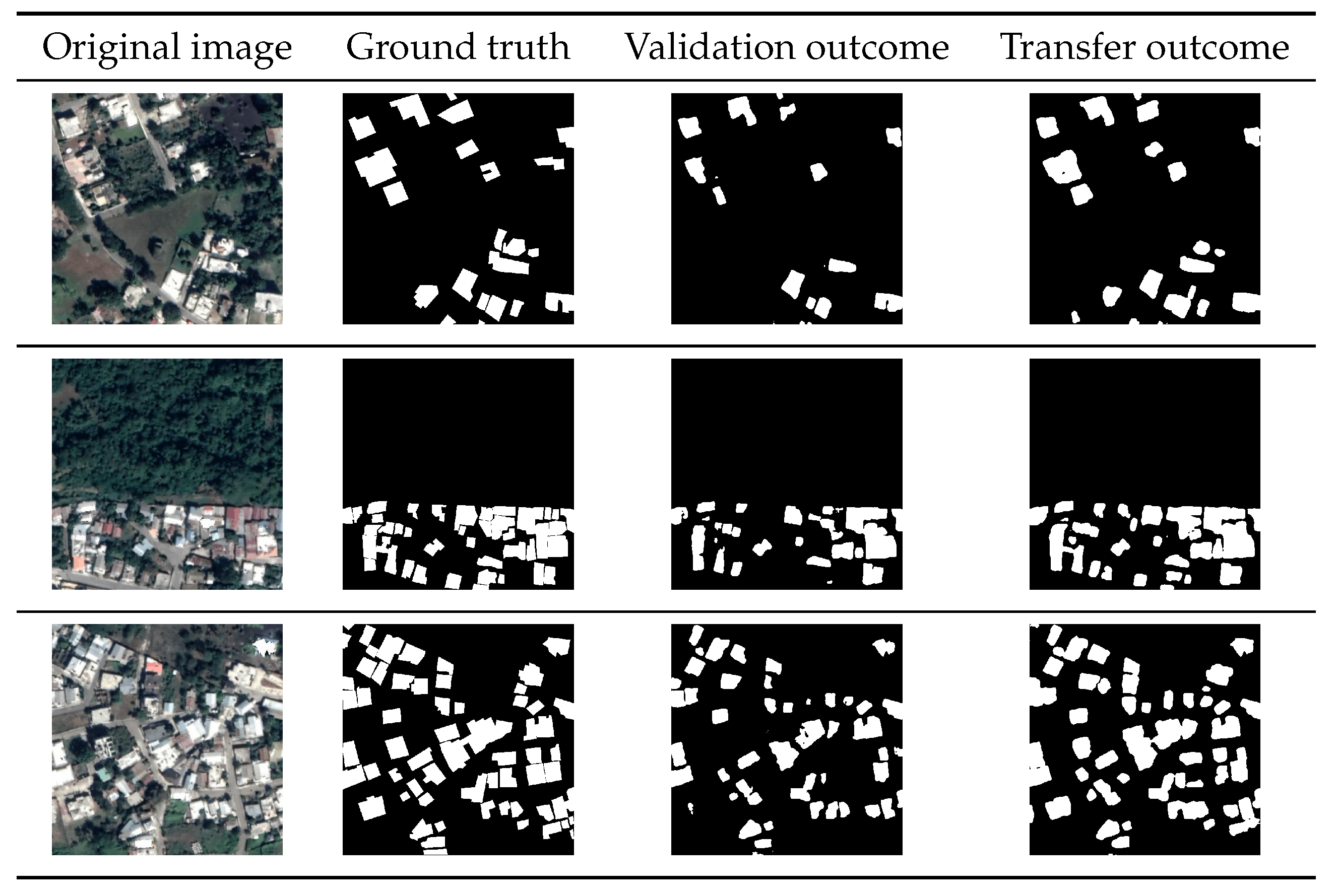
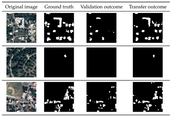
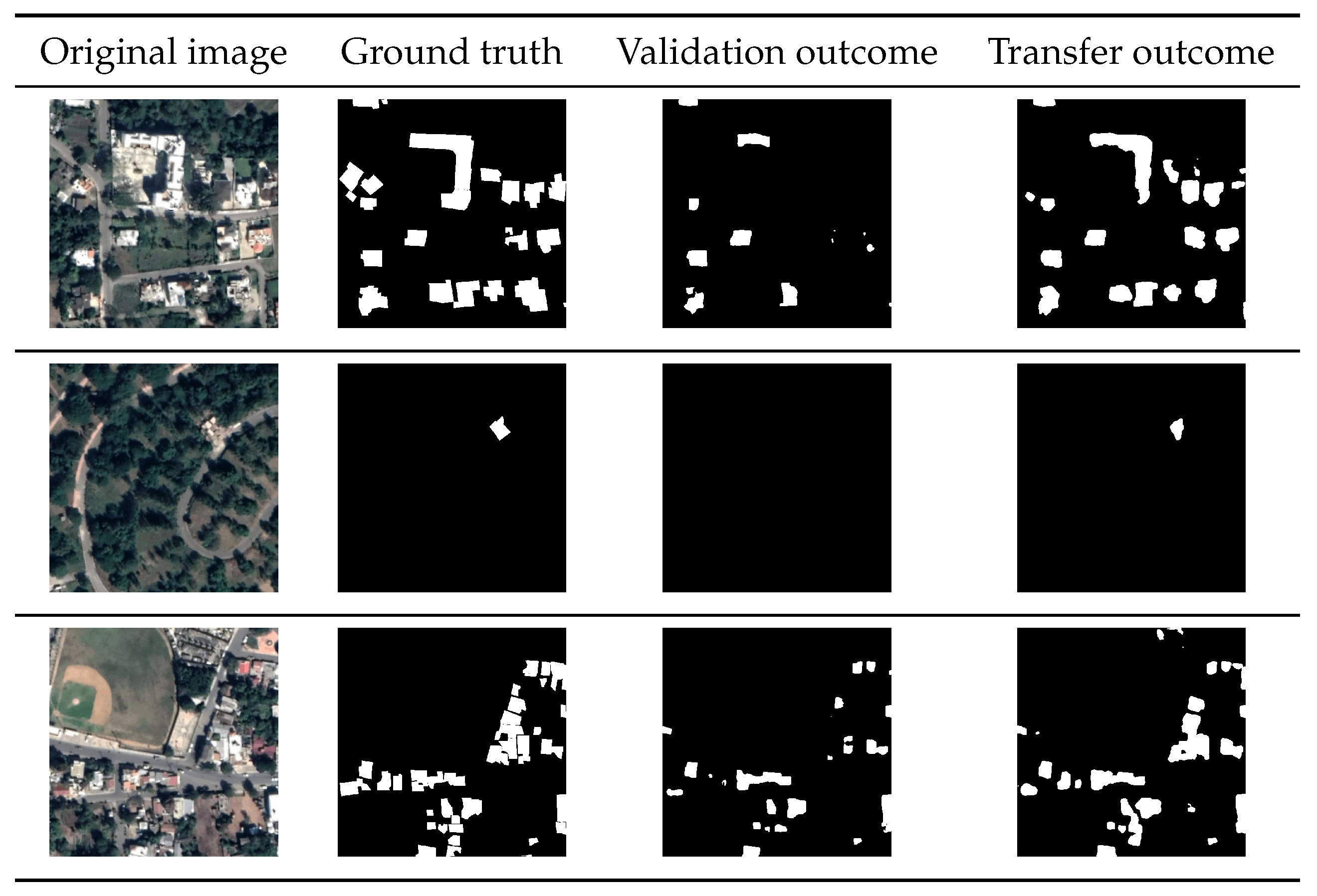
Figure 10 and Figure 11 display representative examples of building detection results applying the soft-voting mechanism for three models: (i) U-Net+ResNeXt50 with Dice cost and an LR of 8 × 10⁻⁵; (ii) U-Net+ResNeXt50 with CEFT_0.25 cost and an LR of 4 × 10⁻⁵; and (iii) U-Net+ResNeXt50 with CEFT_0.25 cost and an LR of 8 × 10⁻⁵. Although validation models were able to extract most of the buildings in Figure 10, outcomes were less accurate for the contexts in Figure 11.

Figure 10. Examples of validation and transfer results: residential buildings distributed in different ways in an environment with vegetation.

Figure 11. Examples of validation and transfer outcomes for different buildings: atypical shapes and sizes, isolated structures, and alongside a baseball field.

5.6.2. Transfer

The last columns in Figure 10 and Figure 11 present the outcome of soft voting for three transfer models: (i) U-Net+ResNet101 with CEFT_0.1 cost, an LR of 4 × 10⁻⁵, and using 50% of the dataset for training; (ii) U-Net+ResNeXt50 with CEFT_0.25 cost and an LR of 4 × 10⁻⁵; and (iii) U-Net+ResNet101 with CEFT_0.25 cost and an LR of 8 × 10⁻⁵ on images from the SJM dataset. Transfer models showed better accuracy than validation models, i.e., the outcomes were more similar to ground truth. For example, transfer models were able to detect the large white building in image #1, correctly identified the isolated building in image #2, and extracted more buildings adjacent to the baseball field in image #3.

5.7. Comparison with Existing Methods for Building Detection

This subsection reports a comparative analysis of the proposed DNNs with state-of-the-art building detection methods.

5.7.1. Baseline Methods and Datasets

Two relevant comparisons were performed. First, the obtained results on standard datasets (including IAD, MBD, WHU, and others) were compared with related works reviewed in Section 2.2. Then, the transfer learning capabilities were compared with existing automated building detection algorithms with publicly available source code over SJM. Four state-of-the-art automatic methods for building detection were considered:

• DlinkNet34 [30], an encoder–decoder DNN including dilated convolution and a pre-trained encoder (Linknet).
• RefiNet [30], a multi-scale refinement DNN that progressively enhances segmentation masks using feature pyramid representations and residual connections.
• The DeeplabV3+ module, [31] which integrates atrous spatial pyramid pooling and a dilated ResNet backbone to capture multi-scale contextual information.
• The Grad-CAM-XAI method [32], using a U-Net architecture combined with gradient-weighted class activation mapping, enabling both segmentation and interpretability by highlighting relevant regions in input images.

The analysis was performed over the SJM dataset, to determine the capabilities of the methods to deal with new, unseen data, in scenarios with a poor urbanistic planning.

5.7.2. Methodology

The DlinkNet34 and RefiNet implementations in the building-footprint-segmentation library [30] and the suggested pre-trained methods were used. The code was adapted to include the extract and run functions for execution on the SJM dataset. Class torch.utils.data.Dataset was used as data loader and iterator.

The DeeplabV3+ module was evaluated using three different pre-trained weights, obtained in training processes over different urban datasets from the crowdAI (www.crowdai.com, accessed on 7 January 2024), SpaceNet (www.spacenet.ai, accessed on 7 January 2024), and urban3d (https://urban3dchallenge.github.io/, accessed on 7 January 2024), repositories. The best $IoU$ results were computed using the weights of the urban3d dataset. A specific variant of the torch.utils.data.Dataset class was used for DeeplabV3+.

Grad-CAM-XAI methods were smoothly integrated by adapting the source project and modifying its visualization tools to support the target dataset metric. In all cases, the $IoU$ metric was computed as described in Section 4.

5.7.3. Results and Samples

Table 4 reports the $IoU$ comparison with previous DNN-based building detection approaches over standard datasets. The last column (${\Delta }_{\mathrm{IoU}}$) summarizes the improvements obtained when applying the proposed soft-voting DNN approach (‘+’ indicates that soft voting computed better results than the corresponding baseline approach).

Table 4. $IoU$ comparison with previous DNN-based building detection approaches.

Article	Method	Dataset	$\mathit{IoU}$ Results	${\Delta }_{\mathbf{IoU}}$
Khryashchev et al. [23]	U-Net, LinkNet	IAD RGB/infrared	0.67	+0.294
Pasquali et al. [44]	U-Net + dual encoders	SpaceNet	0.60 to 0.80	+0.166 to +0.366
Pan et al. [26]	U-Net	aerial imagery + GIS	0.86 to 0.93	+0.036 to +0.106
Ahmed et al. [27]	U-Net	HR images	0.43 to 0.94	+0.026 to +0.536
Jiwani et al. [31]	DeepLabV3+, ResNet	Urban3D, SpaceNet, AICrowd	0.702 to 0.922	+0.044 to +0.264
Li et al. [20]	U-Net, Cascade CNN, Cascade R-CNN	WHU, ISPRS Vaihingen	0.851	+0.114
Liu et al. [34]	U-Net + transformers	AID	0.910	+0.056
Chang et al. [35]	ConvNeXt + BHAT	MBD, WHU, IAD	MBD: 0.765, WHU: 0.918, IAD: 0.827	MBD: +0.201, WHU: +0.048, IAD: +0.139
Yu et al. [45]	Attention U-Net	WHU, IAD	WHU: 0.855, IAD: +0.682	WHU: +0.110, IAD: +0.284

Results in Table 4 indicate that the proposed soft-voting approach computed accurate results, improving over all baseline methods on standard datasets. Notable improvements were obtained over other approaches when applying U-Net (+0.294 over U-Net, LinkNet [23], +0.366 over U-Net + dual encoders [44]) and minor improvements over other sophisticated models (+0.114 over U-Net + Cascade [20], +0.110 to +0.284 over U-Net using attention mechanisms [45]). The obtained results are relevant, considering that only RGB images were used as input, whereas other approaches work on more sophisticated pieces of information (including infrared, LIDAR, and others).

Table 5 reports the average, standard deviation, minimum, maximum, and range of $IoU$ values computed by the proposed approach using U-Net, ResNet, and soft voting, and the four baseline automatic building detection methods considered in the comparison, for the SJM dataset. The average $IoU$ values for the building class are also reported.

Table 5. Comparative $IoU$ results: U-Net+ResNet (soft voting) vs. baseline building detection methods on the SJM dataset.

Model	Average	St. Dev.	Min.	Max.	Range	Building Class
U-Net+ResNet (soft voting)	0.9163	0.0720	0.7592	1.000	0.2408	0.6883
DlinkNet34 [30]	0.7836	0.2541	0.4861	1.000	0.5139	0.1441
RefiNet [30]	0.8180	0.1360	0.5709	1.000	0.4291	0.2646
DeeplabV3+ [31]	0.8247	0.1394	0.5073	1.000	0.4927	0.3270
Grad-CAM-XAI [32]	0.7824	0.1653	0.4618	1.000	0.5382	0.2760

U-Net+ResNet model with soft voting was able to outperform all the baseline building detection methods on the SJM dataset. The average $IoU$ of U-Net+ResNet was 0.9163, i.e., 10% better than the best baseline method (DeeplabV3+). U-Net+ResNet was also the most robust method overall, with an standard deviation of 0.07, half of the best standard deviation of the baseline methods. Regarding the $IoU$ for the building class, the improvements of U-Net+ResNet over the other methods were over 30% in all cases. The proposed soft-voting model properly handled the building detection problem in areas with poor urban planning and significantly outperformed state-of-the-art models.

Table 6 reports the global $IoU$ results (for both classes) and the building class for three problematic scenarios in the SJM dataset (identified by a baseball court, a diagonal street, and sparse houses in the images).

Table 6. Comparative $IoU$ results for problematic scenarios in the SJM dataset.

Scenario	U-Net+ResNet		DlinkNet34 [30]		RefiNet [30]		DeeplabV3+ [31]		Grad-CAM-XAI [32]
	Global	Building	Global	Building	Global	Building	Global	Building	Global	Building
baseball court	0.9102	0.6541	0.5017	0.0726	0.7918	0.1068	0.8094	0.2646	0.7942	0.1512
diagonal street	0.8124	0.6384	0.3102	0.0688	0.6575	0.1922	0.6714	0.2320	0.6069	0.1153
sparse houses	0.8957	0.6652	0.5713	0.0747	0.7096	0.2341	0.8002	0.2029	0.7641	0.0799

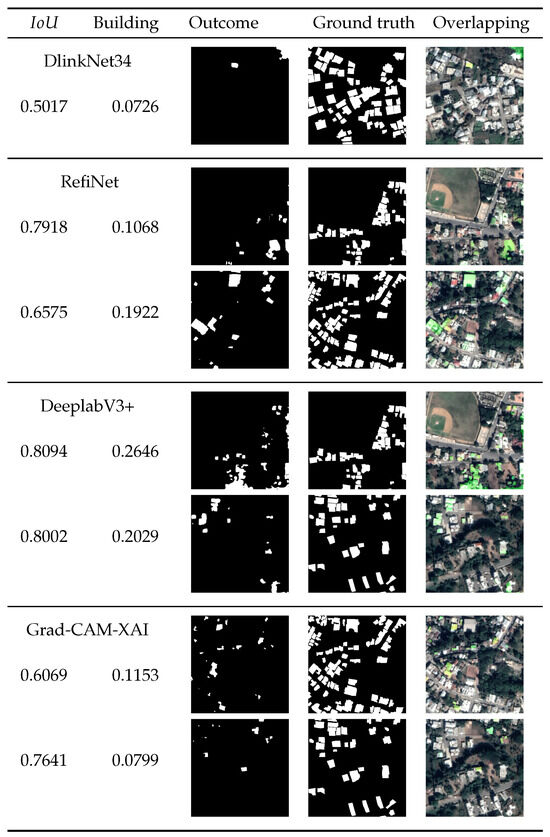
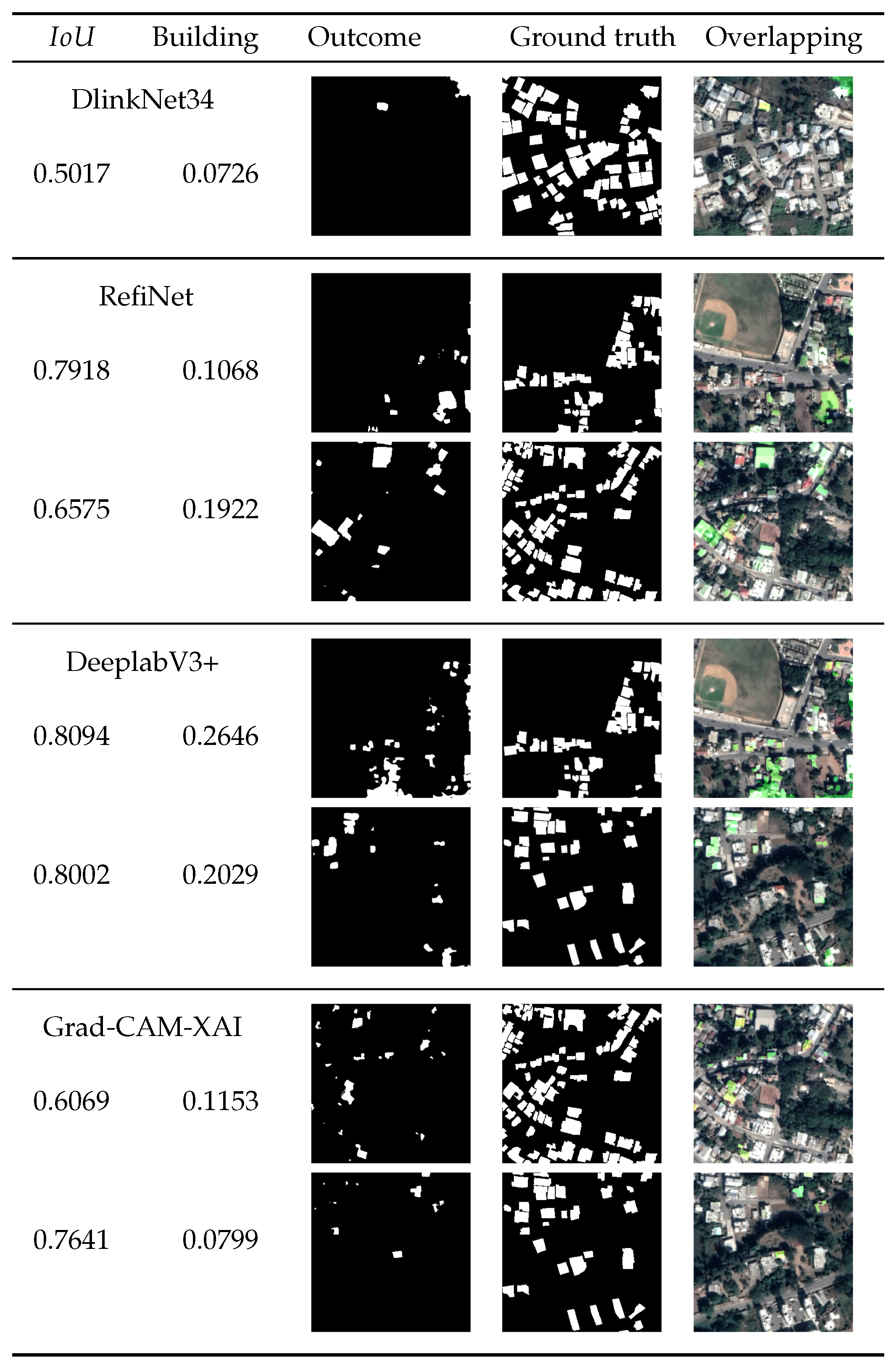
U-Net+ResNet was able to handle those problematic scenarios and computed global $IoU$ values over 0.81 and a maximum of 0.91, whereas the baseline methods fared worst, with $IoU$ values as low as 0.50 and not better than 0.81 in any case. In the building class, the improvements of U-Net+ResNet were noteworthy, with $IoU$ values in the range of 0.65, whereas the baseline methods were below 0.27. Figure 12 presents examples of problematic images that posed a hard challenge to the baseline building detection methods.

Figure 12. Samples of problematic images for the considered baseline methods.

6. Conclusions and Future Work

This article presented a comprehensive methodology for automated building detection using only high-resolution RGB aerial imagery. U-Net and FCN variants with ResNet and ResNeXt backbones were studied and we introduced an ensemble strategy with temperature scaling to enhance predictive robustness.

Unlike many prior studies that rely on multispectral, infrared, or GIS datasets [24,25,29], our approach demonstrates state-of-the-art performance using only RGB inputs. On multiple public datasets, the models achieved Intersection over Union ($IoU$) values exceeding $0.91$ and notably reached $0.9101$ on a newly introduced dataset for San José de las Matas (SJM), an informal urban area characterized by low structural regularity. With calibrated ensemble voting, performance further improved to $0.9163$, surpassing existing methods in both generalizability and efficiency.

This study also contributes a manually annotated, open dataset for SJM, designed to evaluate transferability in underrepresented regions. The SJM dataset addresses a pressing need in geospatial AI research: the lack of benchmarks from informal or low-income urban settlements. Despite promising results, certain limitations remain. The reliance on high-resolution imagery constrains applicability in low-resource settings. Additionally, ensemble-based models, while accurate, increase computational overhead and may require simplification for large-scale or real-time deployment.

Future research will explore the following directions: (i) incorporating advanced DNN architectures such as DeepLabV3 [46], Gated-SCNN [47], and transformer-based networks like Swin Transformers [48] to enhance segmentation accuracy while reducing model complexity; (ii) addressing data imbalance and regional variability through adaptive augmentation strategies and synthetic data generation; and applying the proposed methodology to practical problems, such as population estimation, integrating auxiliary geospatial or temporal data to model dynamic urban analytics and longitudinal studies.

Overall, the proposed methodology provides a scalable, cost-effective solution for building detection, tailored for deployment in real-world, heterogeneous urban environments. It offers a meaningful contribution to the intersection of deep learning, Earth observation, and smart city development.

References

- Donnay, J.; Barnsley, M.; Longley, P. Remote Sensing and Urban Analysis: GISDATA 9; CRC Press: Boca Raton, FL, USA, 2000. [Google Scholar]
- Weng, Q.; Quattrochi, D.A. Urban Remote Sensing; CRC Press: Boca Raton, FL, USA, 2018. [Google Scholar]
- Daranagama, S.; Witayangkurn, A. Automatic building detection with polygonizing and attribute extraction from high-resolution images. ISPRS Int. J. Geo-Inf. 2021, 10, 606. [Google Scholar] [CrossRef] [Scilit]
- Asokan, A.; Anitha, J. Change detection techniques for remote sensing applications: A survey. Earth Sci. Inform. 2019, 12, 143–160. [Google Scholar] [CrossRef] [Scilit]
- Jahan, F.; Zhou, J.; Awrangjeb, M.; Gao, Y. Fusion of hyperspectral and LiDAR data using discriminant correlation analysis for land cover classification. IEEE J. Sel. Top. Appl. Earth Obs. Remote Sens. 2018, 11, 3905–3917. [Google Scholar] [CrossRef] [Scilit]
- Sishodia, R.; Ray, R.; Singh, S. Applications of remote sensing in precision agriculture: A review. Remote Sens. 2020, 12, 3136. [Google Scholar] [CrossRef] [Scilit]
- Doda, S.; Wang, Y.; Kahl, M.; Hoffmann, E.; Taubenböck, H.; Zhu, X. So2Sat POP—A Curated Benchmark Data Set for Population Estimation from Space on a Continental Scale. arXiv 2022, arXiv:2204.08524. [Google Scholar] [CrossRef] [Scilit]
- Mboga, N.; Persello, C.; Bergado, J.R.; Stein, A. Detection of Informal Settlements from VHR Images Using Convolutional Neural Networks. Remote Sens. 2017, 9, 1106. [Google Scholar] [CrossRef] [Scilit]
- Alshawabkeh, Z.; Hasan, A.; Kim, S.C. Identifying Informal Settlements Using Contourlet Assisted Deep Learning. Sensors 2020, 20, 2733. [Google Scholar] [CrossRef] [Scilit]
- Raj, A.; Mitra, A.; Sinha, M. Deep Learning for Slum Mapping in Remote Sensing Images: A Meta-analysis and Review. arXiv 2024, arXiv:2406.08031. [Google Scholar] [CrossRef] [Scilit]
- Li, J.; Huang, X.; Tu, L.; Zhang, T.; Wang, L. A review of building detection from very high resolution optical remote sensing images. GIScience Remote Sens. 2022, 59, 1199–1225. [Google Scholar] [CrossRef] [Scilit]
- Wang, L.; Fang, S.; Li, R.; Meng, X. Building Extraction with Vision Transformer. arXiv 2021, arXiv:2111.15637. [Google Scholar] [CrossRef] [Scilit]
- Liu, H.; Wang, W.; Tang, J.; Deng, M.; Ding, C. A Building Group Recognition Method Integrating Spatial and Semantic Similarity. ISPRS Int. J. Geo-Inf. 2025, 14, 154. [Google Scholar] [CrossRef] [Scilit]
- Goodfellow, I.; Bengio, Y.; Courville, A. Deep Learning; MIT Press: Cambridge, MA, USA, 2016. [Google Scholar]
- Wang, X.; Qian, H.; Xie, L.; Wang, X.; Li, B. Recognition and classification of typical building shapes based on YOLO object detection models. ISPRS Int. J. Geo-Inf. 2024, 13, 433. [Google Scholar] [CrossRef] [Scilit]
- Mnih, V. Road and Building Detection Datasets. Available online: https://www.cs.toronto.edu/~vmnih/data/ (accessed on 7 January 2024).
- Maggiori, E.; Tarabalka, Y.; Charpiat, G.; Alliez, P. Can semantic labeling methods generalize to any city? the INRIA aerial image labeling benchmark. In Proceedings of the IEEE International Geoscience and Remote Sensing Symposium; IEEE: New York, NY, USA, 2017; pp. 3226–3229. [Google Scholar]
- Ji, S.; Wei, S.; Lu, M. Fully building segmentation fromConvolutional Networks for Multi-Source Building Extraction from An Open Aerial and Satellite Imagery Dataset. IEEE Trans. Geosci. Remote Sens. 2018, 57, 574–586. [Google Scholar] [CrossRef] [Scilit]
- González, L.; Toutouh, J.; Nesmachnow, S. Artificial Intelligence for Automatic Building Extraction from Urban Aerial Images. In Smart Cities; Springer Nature: Cham, Switzerland, 2023; pp. 31–45. [Google Scholar]
- Li, Z.; Xin, Q.; Sun, Y.; Cao, M. A deep learning-based framework for automated extraction of building footprint polygons from very high-resolution aerial imagery. Remote Sens. 2021, 13, 3630. [Google Scholar] [CrossRef] [Scilit]
- Minaee, S.; Boykov, Y.; Porikli, F.; Plaza, A.; Kehtarnavaz, N.; Terzopoulos, D. Image Segmentation Using Deep Learning: A Survey. IEEE Trans. Pattern Anal. Mach. Intell. 2022, 44, 3523–3542. [Google Scholar] [CrossRef] [Scilit]
- Ivanovsky, L.; Khryashchev, V.; Pavlov, V.; Ostrovskaya, A. Building Detection on Aerial Images Using U-Net Neural Networks. In Proceedings of the 24th Conference of Open Innovations Association, Moscow, Russia, 8–12 April 2019; pp. 116–122. [Google Scholar]
- Khryaschev, V.; Ivanovsky, L. Urban areas analysis using satellite image segmentation and deep neural network. E3S Web Conf. 2019, 135, 01064. [Google Scholar] [CrossRef] [Scilit]
- Khryashchev, V.; Larionov, R.; Ostrovskaya, A.; Semenov, A. Modification of U-Net neural network in the task of multichannel satellite images segmentation. In Proceedings of the East-West Design & Test Symposium, Batumi, Georgia, 13–16 September 2019; pp. 1–4. [Google Scholar]
- Li, W.; He, C.; Fang, J.; Zheng, J.; Fu, H.; Yu, L. Semantic segmentation-based building footprint extraction using very high-resolution satellite images and multi-source GIS data. Remote Sens. 2019, 11, 403. [Google Scholar] [CrossRef] [Scilit]
- Pan, Z.; Xu, J.; Guo, Y.; Hu, Y.; Wang, G. Deep learning segmentation and classification for urban village using a worldview satellite image based on U-Net. Remote Sens. 2020, 12, 1574. [Google Scholar] [CrossRef] [Scilit]
- Ahmed, N.; Mahbub, R.B.; Rahman, R.M. Learning to extract buildings from ultra-high-resolution drone images and noisy labels. Int. J. Remote Sens. 2020, 41, 8216–8237. [Google Scholar] [CrossRef] [Scilit]
- Singla, J.G.; Ramani, B. Automatic Building Footprint Extraction using Deep Learning. In Proceedings of the International Conference on Computational Intelligence, Communication Technology and Networking; IEEE: New York, NY, USA, 2023; pp. 9–14. [Google Scholar]
- Xu, Y.; Wu, L.; Xie, Z.; Chen, Z. Building extraction in very high resolution remote sensing imagery using deep learning and guided filters. Remote Sens. 2018, 10, 144. [Google Scholar] [CrossRef] [Scilit]
- Robinson, C.; Ortiz, A.; Park, H.; Lozano, N.; Kaw, J.K.; Sederholm, T.; Dodhia, R.; Ferres, J. Fast building segmentation from satellite imagery and few local labels. In Proceedings of the IEEE Conference on Computer Vision and Pattern Recognition, New Orleans, LA, USA, 18–24 June 2022; pp. 1463–1471. [Google Scholar]
- Jiwani, A.; Ganguly, S.; Ding, C.; Zhou, N.; Chan, D.M. A semantic segmentation network for urban-scale building footprint extraction using rgb satellite imagery. arXiv 2021, arXiv:2104.01263. [Google Scholar] [CrossRef] [Scilit]
- Gizzini, A.K.; Shukor, M.; Ghandour, A.J. Extending cam-based xai methods for remote sensing imagery segmentation. arXiv 2023, arXiv:2310.01837. [Google Scholar] [CrossRef] [Scilit]
- Gonzalez, D.; Rueda-Plata, D.; Acevedo, A.B.; Duque, J.C.; Ramos-Pollán, R.; Betancourt, A.; García, S. Automatic detection of building typology using deep learning methods on street level images. Build. Environ. 2020, 177, 106805. [Google Scholar] [CrossRef] [Scilit]
- Liu, G.; Diao, K.; Zhu, J.; Wang, Q.; Li, M. STransU2Net: Transformer based hybrid model for building segmentation in detailed satellite imagery. PLoS ONE 2024, 19, e0299732. [Google Scholar] [CrossRef] [Scilit]
- Chang, J.; Cen, Y.; Cen, G. Asymmetric Network Combining CNN and Transformer for Building Extraction from Remote Sensing Images. Sensors 2024, 24, 6198. [Google Scholar] [CrossRef] [Scilit]
- Xie, S.; Girshick, R.; Dollár, P.; Tu, Z.; He, K. Aggregated Residual Transformations for Deep Neural Networks. In Proceedings of the IEEE Conference on Computer Vision and Pattern Recognition, Honolulu, HI, USA, 21–26 July 2017; pp. 5987–5995. [Google Scholar]
- Long, J.; Shelhamer, E.; Darrell, T. Fully Convolutional Networks for Semantic Segmentation. In Proceedings of the IEEE Conference on Computer Vision and Pattern Recognition, Boston, MA, USA, 7–12 June 2015. [Google Scholar]
- Labelbox. The Data-Centric AI Platform. Available online: https://labelbox.com/ (accessed on 8 March 2024).
- Salehi, S.S.M.; Erdogmus, D.; Gholipour, A. Tversky loss function for image segmentation using 3D fully convolutional deep networks. In Machine Learning in Medical Imaging; Lecture Notes in Computer Science; Springer: Cham, Switzerland, 2017. [Google Scholar]
- González Petti, L.; Nesmachnow, S.; Toutouh, J. Aprendizaje Profundo para la Extracción de Edificios en Ciudades sin Planificación Urbana. Tesis de Grado, Ingeniero en Computación, Universidad de la República (Uruguay). Facultad de Ingeniería, Montevideo, Uruguay, 2021. Available online: https://hdl.handle.net/20.500.12008/34130 (accessed on 10 March 2024).
- Mozafari, A.S.; Siqueira, H.; Leão, W.; Janny, S.; Gagné, C. Attended Temperature Scaling: A Practical Approach for Calibrating Deep Neural Networks. arXiv 2019, arXiv:1810.11586v3. [Google Scholar] [CrossRef] [Scilit]
- Nesmachnow, S.; Iturriaga, S. Cluster-UY: Collaborative Scientific High Performance Computing in Uruguay. In Supercomputing; Communications in Computer and Information Science; Springer: Cham, Switzerland, 2019; Volume 1151, pp. 188–202. [Google Scholar]
- Rojarath, A.; Songpan, W.; Pong-inwong, C. Improved ensemble learning for classification techniques based on majority voting. In Proceedings of the 2016 7th IEEE International Conference on Software Engineering and Service Science (ICSESS), Beijing, China, 26–28 August 2016; IEEE: New York, NY, USA, 2016; pp. 107–110. [Google Scholar]
- Pasquali, G.; Iannelli, G.; Dell’Acqua, F. Building footprint extraction from multispectral, spaceborne earth observation datasets using a structurally optimized U-Net convolutional neural network. Remote Sens. 2019, 11, 2803. [Google Scholar] [CrossRef] [Scilit]
- Yu, M.; Chen, X.; Zhang, W.; Liu, Y. AGs-Unet: Building Extraction Model for High Resolution Remote Sensing Images Based on Attention Gates U Network. Sensors 2022, 22, 2932. [Google Scholar] [CrossRef] [Scilit]
- Chen, L.; Papandreou, G.; Schroff, F.; Adam, H. Rethinking Atrous Convolution for Semantic Image Segmentation. arXiv 2017, arXiv:1706.05587. [Google Scholar] [CrossRef] [Scilit]
- Takikawa, T.; Acuna, D.; Jampani, V.; Fidler, S. Gated-SCNN: Gated Shape CNNs for Semantic Segmentation. arXiv 2019, arXiv:1907.05740. [Google Scholar] [CrossRef] [Scilit]
- Liu, Z.; Lin, Y.; Cao, Y.; Hu, H.; Wei, Y.; Zhang, Z.; Lin, S.; Guo, B. Swin transformer: Hierarchical vision transformer using shifted windows. In Proceedings of the IEEE International Conference on Computer Vision; IEEE: New York, NY, USA, 2021; pp. 10012–10022. [Google Scholar]
Disclaimer/Publisher’s Note: The statements, opinions and data contained in all publications are solely those of the individual author(s) and contributor(s) and not of MDPI and/or the editor(s). MDPI and/or the editor(s) disclaim responsibility for any injury to people or property resulting from any ideas, methods, instructions or products referred to in the content. |
© 2026 by the authors. Published by MDPI on behalf of the International Society for Photogrammetry and Remote Sensing. Licensee MDPI, Basel, Switzerland. This article is an open access article distributed under the terms and conditions of the Creative Commons Attribution (CC BY) license.