Constrained Close Loop Model Predictive Control Architecture for Deformable Linear Objects for Dynamic Motions

Abstract

Deformable linear objects (DLOs) exhibit highly nonlinear dynamic behavior, complicating their control during high-speed maneuvers. Furthermore, the lack of a generic spatial representation and the difficulty of real-time state estimation hinder effective closed-loop manipulation. Building upon our previously established state estimation framework and control architecture, this paper introduces a constrained, closed-loop model predictive control (MPC) approach for highly dynamic DLO manipulation. We integrate hardware and environmental limits into the MPC as soft constraints, enabling tasks like dynamic tracking with endpoint wall avoidance. Additionally, we demonstrate challenging maneuvers, such as swinging a DLO through a narrow slot in open-loop. Furthermore, we enhance our prior state estimation method by incorporating mid-object via points, significantly improving shape reconstruction and enabling the prediction of non-monotonically curved geometries. Finally, we present an extensive evaluation of the complete control architecture using two simulated and five physical DLOs. This analysis assesses the critical influence of kinematic segment discretization, object dynamics, and distribution shifts on overall tracking performance, thereby validating the efficacy and robustness of the approach.

1. Introduction

Manipulating deformable objects remains a highly challenging yet essential aspect of robotics. Challenges arise across the entire application stack, including state representation selection, perception, state estimation, dynamics modeling, control, and the diverse behavioral characteristics of deformable objects [1,2]. Nevertheless, because many common objects are deformable, robots must be capable of controlling objects such as medical needles, tubes, industrial foams, ropes, and cables [1]. These objects belong to a specific category characterized by one dimension being significantly larger than the other two, commonly referred to as deformable linear objects (DLOs).

A common simplification involves interacting with DLOs in a slow-motion regime, where the object moves quasi-statically, rendering the nonlinear effects of deformation dynamics negligible. Conversely, fast motions require accurate state estimation at high frequency, a dynamics model capable of capturing nonlinear deformation dynamics, and a controller that anticipates long-term dynamic behavior while managing the diverse characteristics of these objects.

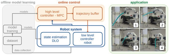
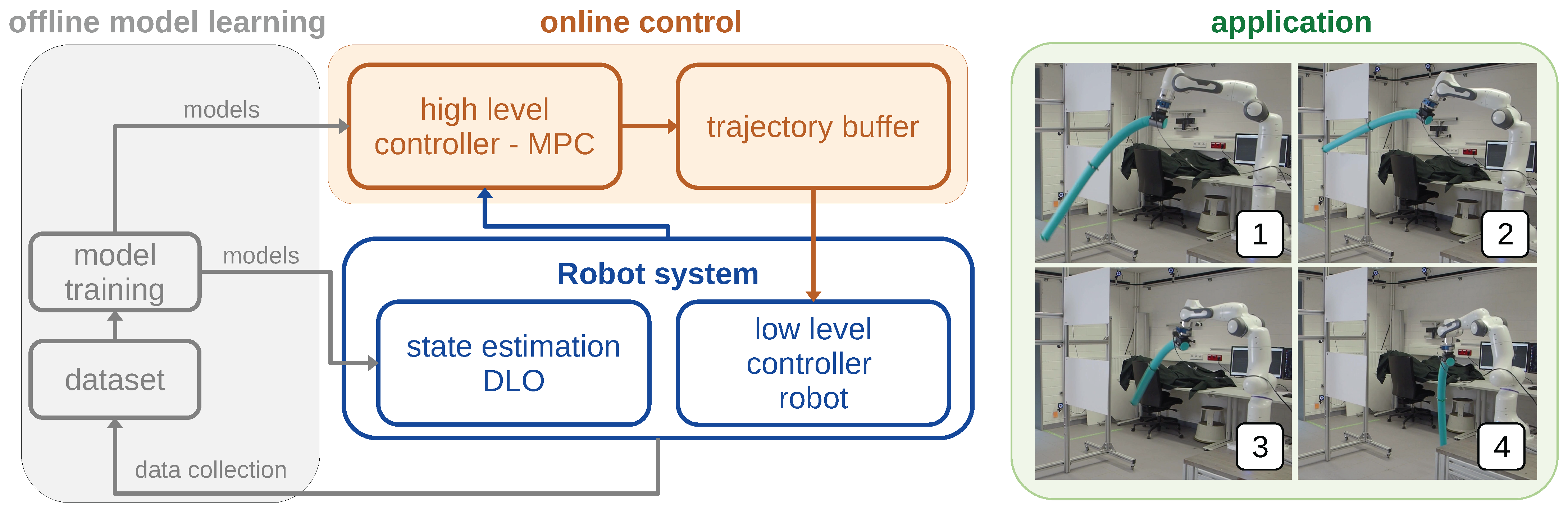
Our research aims to enable constrained closed-loop control of DLOs during dynamic motions, accounting for both hardware and environmental constraints. We target DLOs with a particularly high bending stiffness that maintain a consistent shape, distinguishing them from ropes that exhibit a wide range of configurations. Examples include maneuvering a DLO within a constraint environment or swinging a foam cylinder through a slot, as illustrated in Figure 1.

Figure 1. Overview of the control application architecture presented in [3]. Desired application of a robot swinging the DLO through a slot (trajectory shown in sequence 1–4).

In previous works [3,4], we introduced the preliminary elements of a closed-loop architecture for solving unconstrained trajectory optimization (TO) to track dynamic motions using the DLO tip position. This architecture represents the DLO as a floating-base kinematic chain. State estimation for this chain is performed using a Kalman filter architecture [4], which relies on data-driven inverse kinematics (DDIK) solvers [5] and a data-driven approximation of hybrid dynamics as the dynamics model [6]. These data-driven models are trained on a pre-recorded dataset containing DLO motion data. For closed-loop TO, the coupled robot-DLO dynamical system is formulated into an Optimal Control Problem (OCP), which is solved via Differential Dynamic Programming (DDP). The solved trajectory is then sent to a trajectory buffer, performing interpolation and trajectory blending and tracked via a low-level controller as seen in Figure 1.

However, these early approaches exhibited major shortcomings that prevented the execution of complex motions, such as the swing maneuver illustrated in Figure 1. Specifically, the DDIK solvers relied solely on partial observations of the DLO base and tip, which forced their learning regularization to predict only monotonically curved shapes. This inability to learn general, accurate shape representations and the absence of a constraint-aware Model Predictive Control (MPC) architecture served as a critical bottleneck. Ultimately, this inaccurate shape modeling and lack of constraint handling severely limited generalization to complex configurations and restricted applications that demand high shape accuracy, such as obstacle avoidance.

In this paper, we significantly enhance the approach by introducing crucial advancements that overcome these limitations. First, we improve the state and shape estimation by proposing the use of additional via points, such as the DLO midpoint. This enables the accurate reconstruction and prediction of complex, non-monotonically curved shapes. Second, we integrate closed-loop MPC into our control architecture, extending the unconstrained approach in [3] to solve tasks subject to hardware and environmental constraints.

While our previous works lacked a holistic evaluation of the overall architecture and its underlying parameters, we now present a comprehensive assessment of the complete system. Specifically, we investigate how the physical characteristics of the DLO impact controller performance, and analyze how parameters, such as the number of modeled segments, influence the accuracy of the entire control stack. This extensive experimental study was conducted across two simulated objects and five real DLOs with diverse physical properties. In summary, we provide the following core contributions:

• The incorporation of additional via points to enhance state and shape estimation, enabling accurate prediction of non-monotonically curved DLO shapes.
• Closed-loop control via MPC in the presence of environmental obstacles and hardware limits.
• A comprehensive, in-depth evaluation of the enhanced control application architecture on two simulated and five real-world objects.

The remainder of this paper is structured as follows: Section 2 discusses related works, and Section 3 provides essential background information. Section 4 describes the overall experimental setting. In Section 5, we introduce and evaluate the learning of the inverse kinematics solvers using additional via points and continue in Section 6, evaluating the control architecture in constraint MPC tasks by introducing hardware and environmental constraints. Section 7 provides a comprehensive analysis of the complete control architecture using different real-world objects. Finally, Section 8 concludes the paper.

2. Related Works

While research extensively covers deformable object modeling and control—with broader overviews in [1,2], this section focuses specifically on dynamic DLO control where the quasi-static assumption fails. The components of our control architecture are reviewed in the following subsections: DLO representation and state estimation (Section 2.1), dynamic modeling (Section 2.2), and control design (Section 2.3).

2.1. DLO Modeling and State Estimation

Under the rigid-body assumption, objects are uniquely defined by a 6D pose in space. Deformable objects lack this generic spatial representation, motivating the development of diverse methods to model their shape and configuration. Mesh representations are among the most powerful and commonly used methods for modeling deformable objects. In [7,8], mesh representations are used to model various foam materials for dynamic manipulation and whipping, respectively. Mesh models are preferred when high state accuracy is required, but this accuracy comes at the cost of high dimensionality and state estimation challenges. For instance, neither [7] nor [8] employs active state estimation; instead, they initialize experiments from known starting configurations. Furthermore, highly accurate object representations demand a large number of modeled degrees of freedom (DoFs), specifically mesh nodes. The authors of [8] utilized 68 to 160 nodes, depending on the object, while [7] employed a significantly larger dimension of 1472 nodes.

Alternative configurational representations can significantly reduce dimensionality and facilitate sufficient state estimation. For example, refs. [9,10] used spatial curves and differential geometry to describe the shape of the DLO backbone. In [9], they employed a polynomial curvature functional parameterization and a Taylor expansion to reduce the state dimension from infinite to a finite degree, dependent on the number of expansion terms. To estimate the object’s state, they utilized a camera-based system operating at 30 Hz to extract target points at the base, midpoint, and tip. These points were mapped into a 2D Cartesian space and processed algorithmically.

In this work, a floating-base kinematic chain representation is used. Here, the number of DoFs corresponds to the joints forming the chain, which often provides reasonably accurate representations with fewer DoFs. In [11,12], the authors modeled the DLO as a kinematic chain composed of rigid cylindrical segments connected by ball joints. For hardware experiments, ref. [11] used a five-cylinder chain, substantially reducing the state dimensionality. Both works employed image-based sensors to capture a DLO point cloud. While [11] conducted final experiments in an open-loop fashion, ref. [12] used the point cloud as input to an observer.

This paper adopts the state representation and estimation framework introduced in [4,5], which utilizes a floating-base kinematic chain model with 2D rotational joints between segments, neglecting axial rotations along the links to reduce each joint by one DoF. These approaches utilized a tracking system to measure base and tip positions, training a DDIK solver to map task-space observations into the joint space of the kinematic chain [5]. In [4], a Kalman filter operating in joint space was proposed to estimate states from multiple DDIK sources, ensuring reliable state estimation. Compared to the camera-based approach in [11], tracking systems provide significantly higher measurement frequencies (approximately 240 Hz); by incorporating the Kalman filter, the state estimation frequency can be further increased to 1 kHz.

While most works employ a physically meaningful state representation, ref. [13] utilized a black-box approach. The authors learned the DLO dynamics using a Recurrent Neural Network (RNN) and initialized all experiments from a common configuration, allowing the DLO state to be implicitly represented by the RNN’s hidden state. They tracked the DLO tip position and applied an extended Kalman filter to estimate this hidden state. While this black-box representation is powerful for control applications, it precludes the introduction of state constraints and provides no explicit shape information.

2.2. Dynamic Modeling

DLO dynamics are notoriously difficult to model due to complex nonlinear effects, including hyperelasticity, viscoelasticity, plasticity, anisotropy, and incompressibility [2]. Consequently, most approaches require parameter identification procedures or utilize machine learning methods.

First-principle models, such as those in [8,9,10], frequently employ parameter identification methods. In [9], the authors estimated dynamic parameters, such as the spring and damping coefficients of their strain model. In [8], the authors used a Finite Element Method (FEM) model based on a mesh representation and a Neo-Hookean material law, estimating the model parameters using experimental data. The authors of [8] note that identifying parameters for dynamic motions remains significantly more challenging than identifying quasi-static parameters.

To address this challenge, learning techniques are frequently employed to represent the object’s dynamics using a universal function approximator. Previous works [4,5] learned DLO dynamics using a floating-base kinematic chain approximation, training various neural network architectures to predict dynamics within the model’s joint space. They utilized a discrete mapping from the current joint state to the next, providing the DLO base trajectory as a network input. Following a similar approach, ref. [14] utilized a hybrid method where the chain was represented by a pseudo-rigid-body model, identifying both dynamic parameters and spring-damper coefficients from data. The hybrid dynamics algorithm [6], which is a combination of inverse and forward dynamics, is then applied to numerically integrate the DLO state based on the base trajectory of the kinematic chain. To account for remaining model mismatches, a small Multi-Layer Perceptron (MLP) was trained to predict residual torques, thereby improving prediction performance.

In this work, we adopt the approach from our previous study [3], where the complete hybrid dynamics function was approximated via a single MLP to eliminate the need for explicit parameter identification. This provides a reasonable tradeoff between high dynamic modeling accuracy, fast evaluation, and the rapid differentiation required for MPC.

2.3. Control

The majority of existing works [3,9,11,12,13] aim to control the DLO endpoint via a fixed grasp at its base, while a few target multiple grasping or contact locations [7,8].

In [12], a model-based kinematic trajectory controller was developed to track the DLO shape utilizing point cloud feedback. In [11], a nonlinear, partially input–output linearizing controller was proposed to handle DLO tip position tracking in dynamic scenarios using the equations of motion. Both works utilized a physics engine for simulation, which natively handles physical collision constraints; however, no additional constraints were explicitly introduced. These instantaneous controllers are specialized functions that do not utilize optimization-based techniques, limiting their ability to incorporate more diverse constraints.

Optimization-based control laws were employed in [7,9]. In [9], a high-level controller solved a model-constrained nonlinear optimization problem for feedforward shape regularization, which was then executed by a low-level PD controller. To ensure feasible solutions, they introduced constraints on the DLO’s floating-base coordinates. In [7], soft barrier functions were used to avoid robot self-collisions and to enforce joint limits. All of these works rely on instantaneous controllers that operate solely on sensor feedback and the system model at the current time step.

MPC offers a powerful alternative by combining optimization with model preview, incorporating the future impact of control actions to better account for nonlinear and time-delayed object behaviors. In [13], an MPC problem was formulated using a learned RNN model to track dynamic 2D DLO shapes in space. They solved the MPC problem using gradient descent without introducing additional state constraints. Because the RNN hidden state serves as an abstract representation of the DLO, straightforward integration of physical constraints is not possible. In [8], offline trajectory optimization was used to plan and execute a path for the DLO tip. Here, constraints such as state and control limits could be introduced via interior-point methods. However, the underlying computationally expensive FEM model complicates real-time closed-loop control, and no online state estimation was performed. Further, ref. [10] demonstrated MPC for rigid–soft systems using the Differentiable Geometrically Variable Strain approach, but their evaluation was limited to simulation, leaving validation on physical hardware as an open challenge.

We addressed these limitations in [3], leveraging the high-frequency state estimation from [4] to perform closed-loop TO, albeit without considering additional constraints. In this work, we extend the approach of [3] by introducing constraints that account for both robot hardware limits and environmental obstacles. Furthermore, the solver and model have been improved to significantly reduce computation time, enabling closed-loop MPC.

3. Background

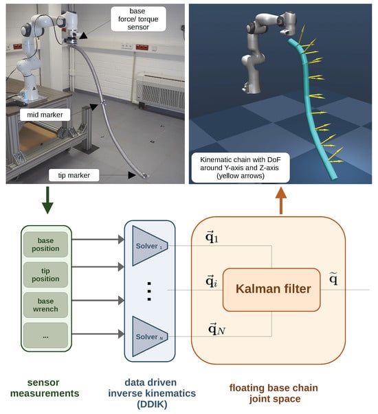
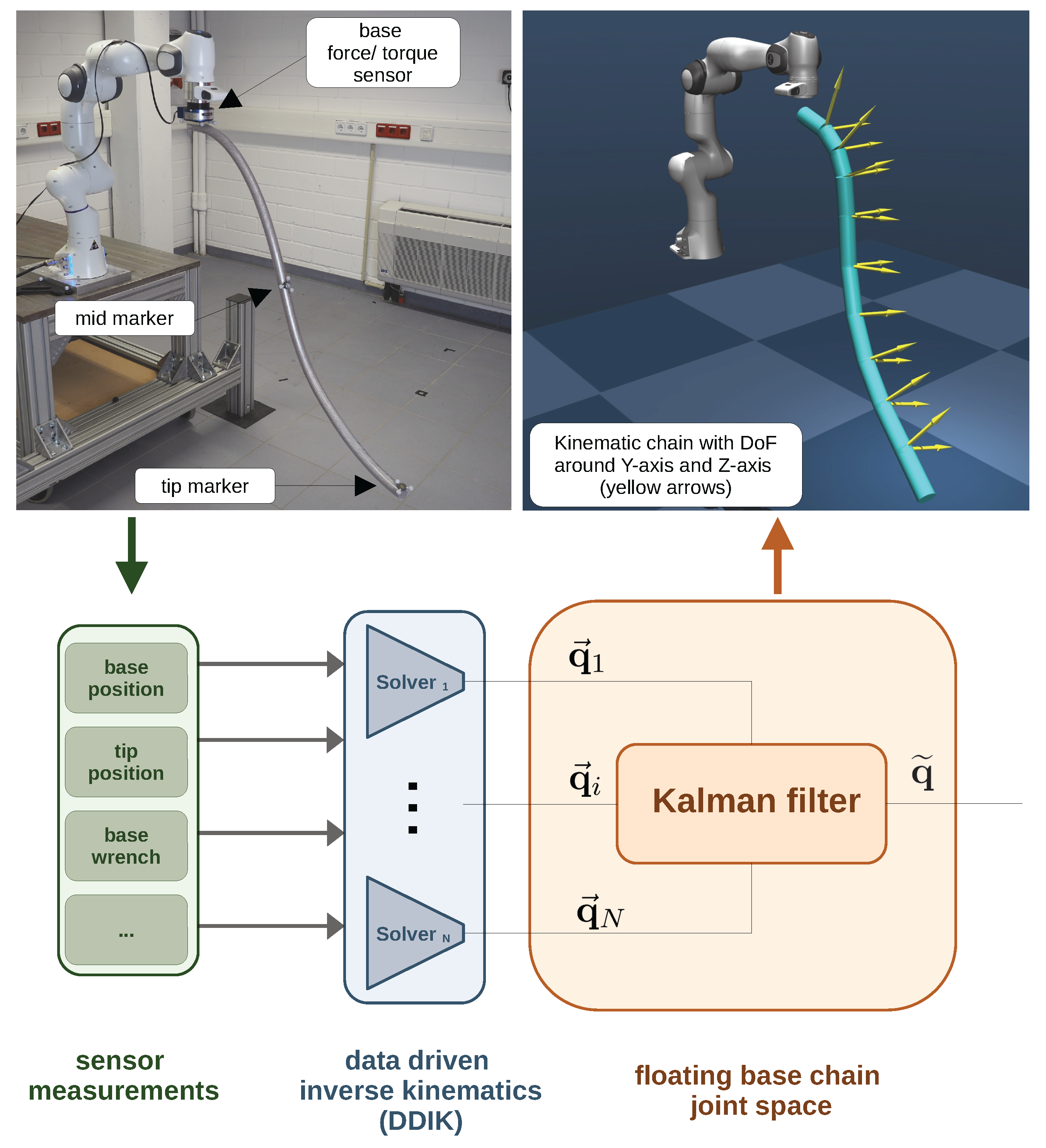
This section introduces relevant information about the components of the control application architecture of [3]. The DLO is modeled as a floating-base kinematic chain with its full state defined as $\overrightarrow{\mathbf{s}}=\left[\overrightarrow{\mathbf{x}},\overrightarrow{\mathbf{q}}\right]$. The floating-base state $\overrightarrow{\mathbf{x}}$ comprises the base pose $\mathbf{x}$ and its spatial velocity $\dot{\mathbf{x}}$, while the joint state $\overrightarrow{\mathbf{q}}$ consists of the positions $\mathbf{q}$ and velocities $\dot{\mathbf{q}}$ of the joints forming the kinematic chain, as illustrated in Figure 2.

Figure 2. Modeling the DLO as a floating-base kinematic chain and estimating its state via Kalman filtering, as introduced in [4]. Figure adapted from [3].

First, the state of the kinematic chain model $\overrightarrow{\mathbf{s}}$ is predicted using various DDIK solvers. Based on these predictions, a Kalman filter estimates the DLO state $\overrightarrow{\mathbf{s}}$. Second, the dynamics of the representative kinematic chain model are formulated using a data-driven approximation of hybrid dynamics. Throughout this work, the DLO base state $\overrightarrow{\mathbf{x}}$ is assumed to be continuously available, for instance, via the forward kinematics of the grasping robot manipulator. The following sections provide a brief overview of the DDIK approach, state estimation, dynamics modeling, and the control strategy.

3.1. State Estimation via Kalman Filter

In [4], we proposed a multichannel sensor-fusion-based approach for state estimation. Multiple DDIK solvers, referred to as encoders, predict the current joint state ${\overrightarrow{\mathbf{q}}}_i$ of the kinematic chain based on various observations of the DLO. This encoder-based, data-driven inverse kinematics was introduced in [5], utilizing partial observations of the DLO base state $\overrightarrow{\mathbf{x}}$ and the DLO tip state $\overrightarrow{\mathbf{t}}$. In [4], the inverse kinematics additionally incorporated the DLO base state $\overrightarrow{\mathbf{x}}$ and the wrench acting at the DLO base ${\mathbf{F}}_b$. The distinct joint state predictions were then provided as inputs to a linear Kalman filter to estimate the overall joint state $\overrightarrow{\tilde{\mathbf{q}}}$.

This Kalman filtering approach requires the encoders to map into a shared joint space. Consequently, ref. [4] proposed training a single teacher encoder that learns a mapping from the observations to a joint space. During training, not only is the encoder trained, but the optimal individual segment lengths of the kinematic chain model are also identified. The cost function comprises three components:

$$\mathcal{L}={\displaystyle \frac{1}{N}}{\displaystyle \sum _{j=1}^N}({\mathcal{L}}_{pred,j}+{\mathcal{L}}_{req,j}+{\mathcal{L}}_{FK}),$$

(1)

where N is the number of data points. The ${\mathcal{L}}_{pred,j}$ accounts for the loss of predicting the tip position correctly.

$${\mathcal{L}}_{pred,j}=w_k{\parallel {\overrightarrow{\mathbf{t}}}_j-{\widehat{\overrightarrow{\mathbf{t}}}}_j\parallel }_{{\mathbf{W}}_{\mathbf{y}}}^2,$$

(2)

where $w_k$ is the weight for the ${\mathbf{W}}_{\mathbf{y}}$ weighted error of the predicted tip state ${\widehat{\overrightarrow{\mathbf{t}}}}_j$ and the true tip state ${\overrightarrow{\mathbf{t}}}_j$.

The kinematic chain representing the DLO is mostly highly redundant, such that multiple predicted joint configurations ${\widehat{\mathbf{q}}}_j$ can yield identical positions of the tip ${\widehat{\overrightarrow{\mathbf{t}}}}_j$. Therefore, ${\mathcal{L}}_{reg,j}$ regularizes the predicted latent joint states by adding a prior toward smaller joint positions and velocities, which resolves this redundancy by consistently favoring the minimum-norm configuration among all configurations consistent with the observations.

$${\mathcal{L}}_{req,j}={\alpha }_q\parallel {\widehat{\mathbf{q}}}_j{\parallel }_2^2+{\alpha }_{\dot{q}}{\parallel {\widehat{\dot{\mathbf{q}}}}_j\parallel }_2^2,$$

(3)

where ${\alpha }_q$ is the regularization weight for the squared 2-norm of the predicted latent joint positions ${\widehat{\mathit{q}}}_{\mathit{j}}$, and ${\alpha }_{dq}$ for the predicted joint velocities ${\widehat{\dot{\mathit{q}}}}_{\mathit{j}}$. We use the following ${\mathcal{L}}_{FK}$ term that regularizes the identification of the segment lengths ${\Theta }_{el}$ of the latent kinematic chain model:

$$\begin{array}{cc}\hfill {\mathcal{L}}_{FK}=& {\alpha }_L(\sum {\Theta }_{el}-L)+{\alpha }_{el}{\parallel {\Theta }_{el}-{\Theta }_{el}^{\prime }\parallel }_2^2\hfill \end{array}$$

(4)

where ${\alpha }_L$ weights the error of the sum of the individual segment lengths $\sum {\Theta }_{el}$ from the actual DLO length L. The scalar ${\alpha }_{el}$ weights the deviation from the initial segment lengths ${\Theta }_{el}^{\prime }$.

After training the teacher encoder model and identifying the segment lengths of the kinematic chain model, all subsequent encoders must map to this shared joint space and optimally predict identical joint states at any given instant. This alignment is achieved by training the student encoders using the following loss function:

$$\begin{array}{cc}\hfill {\mathcal{L}}_s=& {\displaystyle \sum _{j+1}^N}{w}_y\parallel {\overrightarrow{\mathbf{t}}}_j-{\widehat{\overrightarrow{\mathbf{t}}}}_j{\parallel }_2^2+{\mathbf{W}}_{q,rec}{\parallel {\widehat{\overrightarrow{\mathbf{q}}}}_{t,j}-{\widehat{\overrightarrow{\mathbf{q}}}}_{s,j}\parallel }_2^2,\hfill \end{array}$$

(5)

where $w_y$ is the weight for the estimated tip state error, ${\mathbf{W}}_{q,rec}$ is the weighting matrix for the reconstruction error of the teacher’s ${\widehat{\overrightarrow{\mathbf{q}}}}_{t,j}$ and the student’s joint states ${\widehat{\overrightarrow{\mathbf{q}}}}_{s,j}$, respectively.

A Kalman filter is employed to estimate the current joint state, utilizing the teacher and student encoder predictions as measurements during the update step. However, a dynamics model of the DLO is still required for the prediction step.

3.2. Dynamics Modeling

Following our earlier approach in [3], this study builds upon the data-driven approximation of hybrid dynamics developed for DLO modeling. In hybrid dynamics, the accelerations of certain joints are known, requiring the computation of the corresponding generalized forces, while for the remaining joints, the generalized forces are given and the resulting accelerations must be computed [6]. Throughout this study, the base acceleration of the DLO is known, and the objective is to calculate both the resulting wrench at the DLO base and the joint accelerations of the kinematic chain:

$$\left[\begin{array}{c}{\mathbf{F}}_b\\ {\ddot{\mathbf{q}}}_{joints}\end{array}\right]={\mathbf{F}}_{HD}\left(\left[\begin{array}{c}\overrightarrow{\mathbf{x}}\\ \overrightarrow{\mathbf{q}}\end{array}\right],\left[\begin{array}{c}{\ddot{\mathbf{x}}}_{base}\\ {\tau }_{joints}\end{array}\right]\right)$$

(6)

Hybrid dynamics requires precise knowledge of the dynamic parameters of the rigid bodies as well as the acting joint torques. These parameters are challenging to identify and may fail to capture the full nonlinear dynamics of a DLO. Therefore, this entire function is approximated by a neural network:

$$\left[\begin{array}{c}{\mathbf{F}}_b\\ {\ddot{\mathbf{q}}}_{joints}\end{array}\right]=\mathbf{NN}\left(\left[\begin{array}{c}\overrightarrow{\mathbf{x}}\\ \overrightarrow{\mathbf{q}}\\ {\ddot{\mathbf{x}}}_{base}\end{array}\right]\right),$$

(7)

By this approximation, the joint state trajectory can be rolled out over time by the DLO base state $\overrightarrow{\mathbf{x}}$, the current joint state $\overrightarrow{\mathbf{q}}$ and DLO base acceleration ${\ddot{\mathbf{x}}}_{base}$.

The loss function for learning the data-driven approximation of hybrid dynamics for a single trajectory is defined by:

$$\begin{array}{cc}\hfill {\mathcal{L}}_{dyn}={\displaystyle \frac{1}{2T}}{\displaystyle \sum _{t=1}^T}& \left(\parallel {\widehat{\overrightarrow{\mathbf{q}}}}_t-{\overrightarrow{\mathbf{q}}}_{\mathrm{ref},t}{\parallel }_{{\mathbf{W}}_{\mathbf{q},\mathbf{t}}}^2+{\parallel {\widehat{\overrightarrow{\mathbf{t}}}}_t-{\overrightarrow{\mathbf{t}}}_{\mathrm{ref},t}\parallel }_{{\mathbf{W}}_{\overrightarrow{\mathbf{t}},\mathbf{t}}}^2\right)+{\parallel {\widehat{\overrightarrow{\mathbf{F}}}}_b-{\overrightarrow{\mathbf{F}}}_b\parallel }_{{\mathbf{W}}_F}^2\hfill \end{array}$$

The first part of the loss is a sum over the whole trajectory of the reconstruction error of the predicted joint space state ${\widehat{\overrightarrow{\mathbf{q}}}}_t$ and the reference joint state ${\overrightarrow{\mathbf{q}}}_{\mathrm{ref},t}$, which is obtained via the data-driven inverse kinematics solvers of Section 3.1, and the tip state error of the predicted tip state ${\widehat{\overrightarrow{\mathbf{t}}}}_t$ and the real tip state ${\overrightarrow{\mathbf{t}}}_{\mathrm{ref},t}$. Further, the acting base wrench at the current time step can be learned using the ${\mathbf{W}}_{\mathbf{F}}$ weighted square norm of the measured base wrench ${\overrightarrow{\mathbf{F}}}_b$ and the predicted base wrench ${\widehat{\overrightarrow{\mathbf{F}}}}_b$.

3.3. Optimal Control Problem

The DLO is modeled as a second-order system, where the state vector $\overrightarrow{\mathbf{s}}$ of the kinematic chain model is integrated over time using the following differential equation [3]:

$$\begin{array}{cc}\hfill \overrightarrow{\dot{\mathbf{s}}}& =\mathbf{f}(\overrightarrow{\mathbf{s}},\overrightarrow{\mathbf{u}})\hfill \\ \hfill \left[\begin{array}{c}\dot{\mathbf{x}}\\ \ddot{\mathbf{x}}\\ \dot{\mathbf{q}}\\ \ddot{\mathbf{q}}\end{array}\right]& =\left[\begin{array}{c}\dot{\mathbf{x}}\\ \overrightarrow{\mathbf{u}}\\ \dot{\mathbf{q}}\\ \mathbf{NN}(\overrightarrow{\mathbf{x}},\overrightarrow{\mathbf{q}},\overrightarrow{\mathbf{u}})\end{array}\right]\hfill \end{array}$$

(8)

where we only consider the predicted joint acceleration ${\ddot{\mathbf{q}}}_{joints}$ of the $\mathbf{NN}(\overrightarrow{\mathbf{x}},\overrightarrow{\mathbf{q}},\overrightarrow{\mathbf{u}})$ network. The control input $\overrightarrow{\mathbf{u}}$ is the floating-base acceleration $\ddot{\mathbf{x}}$.

Based on the state vector $\overrightarrow{\mathbf{s}}$, we want to solve the optimal control problem of the following form:

$$\begin{array}{cc}\hfill {\overrightarrow{{\mathbf{u}}^{\ast }}}_{t:t+N-1}=& \underset{{\overrightarrow{\mathbf{u}}}_{t:t+N-1}}{argmin}{\displaystyle \frac{1}{2}}\left({\overrightarrow{\mathbf{e}}}_N^T\mathbf{T}{\overrightarrow{\mathbf{e}}}_N\right)+{\displaystyle \frac{1}{2}}{\displaystyle \sum _{i=1}^{N-1}}\left({\overrightarrow{\mathbf{e}}}_i^T\mathbf{S}{\overrightarrow{\mathbf{e}}}_i+{\overrightarrow{\mathbf{u}}}_i^T\mathbf{R}{\overrightarrow{\mathbf{u}}}_i\right)\hfill \\ \hfill \mathit{such}& \mathit{that}:\mathbf{H}\left({\overrightarrow{\mathbf{s}}}_j\right)=0,\mathbf{G}\left({\overrightarrow{\mathbf{s}}}_j\right)\ge 0\hfill \\ \hfill & \mathit{with}:{\overrightarrow{\mathbf{e}}}_j={\overrightarrow{\mathbf{s}}}_j-{\overrightarrow{\mathbf{s}}}_{\mathrm{goal},j}\forall j=1,\dots ,N\hfill \end{array}$$

(9)

Here, ${\overrightarrow{\mathbf{s}}}_{\mathrm{goal},j}$ is the desired state at time index t. ${\mathbf{u}}_i$ is the control input, in our case, the floating base acceleration, while $\mathbf{S}$ and $\mathbf{R}$ are weighting matrices and $\mathbf{T}$ is the conventional terminal weight for the final state ${\overrightarrow{\mathbf{s}}}_{t,N}$. The functions $\mathbf{H}\left(\right)$ and $\mathbf{G}\left(\right)$ introduce constraints to the optimization problem.

4. Experimental Setting and Implementation

The following evaluations are performed using simulation and hardware experiments. The experimental robotic platform is a 7-DoF Franka robotic arm.

4.1. Experimental Setting

Simulation: In the Gazebo simulation, we model the DLO as a six-segment kinematic chain with lengths of 0.1 m, 0.1 m, 0.1 m, 0.2 m, 0.2 m and 0.3 m. We model two DLOs: one relatively stiff and the other relatively soft. To achieve appropriate deformation behavior, the dynamics are governed by heuristically tuned spring-damper parameters at the kinematic chain joints.

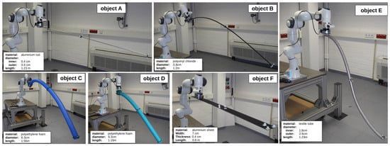
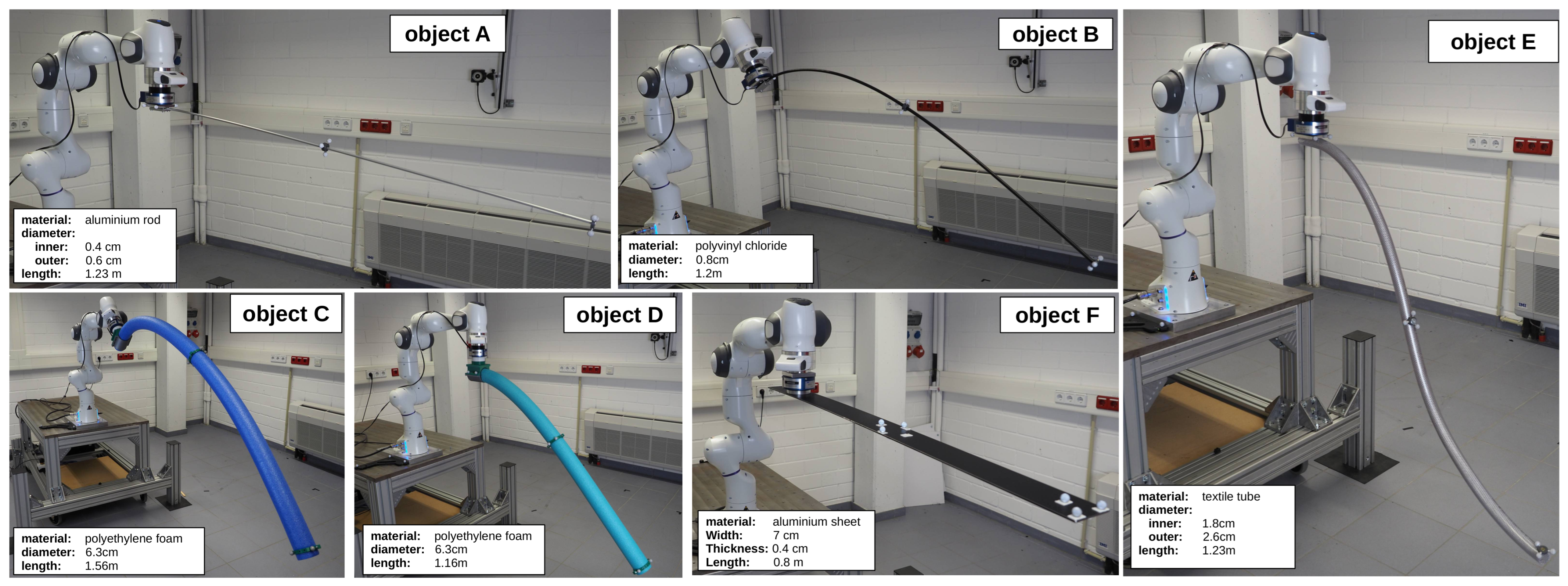
Hardware: We evaluate the approach using five different DLOs (A–E), as depicted in Figure 3, while object F is reserved for proof-of-concept validation. These objects exhibit a wide range of physical properties, from relatively rigid (object A) to highly flexible (object B). Additionally, object E features a non-monotonically curved shape. Reflective markers are attached to the objects to visually track the base, mid, and tip positions of the DLO using an OptiTrack motion capture system. Furthermore, a JR3 85M35A-140-D 200N12 force-torque sensor measures the wrench between the robot and the DLO base.

Figure 3. Overview of used DLO test objects.

Data Collection: We collect data from the simulated and physical objects by executing 40 randomly sampled sinusoidal joint trajectories. Each trajectory consists of an initial 2 s wait time, a 15 s moving period, and a 7 s resting phase. Each movement incorporates a smooth 4 s ramp-up and ramp-down phase. Of the 40 recorded trajectories, 10 were held out for later evaluation. The remaining 30 trajectories were divided into training and validation sets using an 80–20 split.

Data Preparation: All measured poses are transformed into a common reference frame, chosen as the robot base frame. Derivatives of unmeasurable quantities are calculated using central differences and smoothed via a rolling average with an adjusted window size.

Shape Tracking: The dynamic tracking of the tip position is evaluated using three different reference shapes with different shape completion times for slow, middle and fast reference motions: A Lissajous figure with a shape duration of 1.9 s, 2.25 s and 4.0 s; a rectangular shape with a shape duration of 1.25 s, 1.75 s and 4.0 s and finally a circle with shape durations of 1.25 s, 1.5 s and 2.2 s.

4.2. Implementation

The neural networks are trained in Python 3.12 using JAX [15] and the FLAX library [16]. The networks utilize a tanh activation function. The neural network representing the DLO dynamics model is trained using a time step of 10 ms over a horizon of $N=100$ steps.

The Kalman filter for state estimation is implemented in C++ and runs at 1 kHz. It utilizes data-driven inverse kinematics solvers and a DLO dynamics network, which are trained with a time step of 1 ms over a horizon of $N=100$. The state estimation parameters of the Kalman filter, such as the covariance matrices, are tuned via hyperparameter optimization.

5. Enhanced State Estimation via Additional Marker

This section introduces the incorporation of additional marker information into the training of the data-driven inverse kinematics solver to better account for the complete shape of the DLO.

5.1. Methodology

The loss function (1) must be adapted to accommodate one or more additional markers. The prediction loss ${\mathcal{L}}_{pred}$ is augmented by a sum to account for the prediction of M additional points:

$${\mathcal{L}}_{pred,j}+={\displaystyle \sum _i^M}\left(w_{m,i}{\parallel {\overrightarrow{\mathbf{m}}}_{i,j}-{\overrightarrow{\widehat{\mathbf{m}}}}_{i,j}\parallel }_{{\mathbf{W}}_{m,i}}^2\right)$$

(10)

where $w_{m,i}$ is the weight for the ${\mathbf{W}}_{m,i}$ weighted error of the predicted via point position ${\overrightarrow{\widehat{\mathbf{m}}}}_{\mathbf{i},\mathbf{j}}$ from the true via point position ${\overrightarrow{\mathbf{m}}}_{\mathbf{i},\mathbf{j}}$.

The locations of the additional markers are computed using the forward kinematics function, considering only the segment length up to each marker’s position. We introduce a factor ${\gamma }_{mid}$ representing the fractional position of the marker along the total length of the DLO to account for inaccurate physical attachment of the markers. This factor is identified during the training process. Consequently, ${\mathcal{L}}_{FK}$ is augmented by:

$$\begin{array}{c}\hfill {\mathcal{L}}_{FK}+={\displaystyle \sum _i^M}\left({\alpha }_{f,i}{\parallel {\gamma }_{mid,i}-{\gamma }_{init,i}\parallel }_2\right)\end{array}$$

(11)

where ${\alpha }_{f,i}$ is the weighting factor regularizing the L2 norm from the current mid-factor ${\gamma }_{mid,i}$ from the initial value ${\gamma }_{init,i}$ for a particular via point.

The loss function for the student encoder remains as defined in Section 3.1. However, additional marker locations can be incorporated using the same technique.

5.2. Evaluation: Enhanced State Estimation

We evaluate our approach for incorporating additional via points by training three encoder networks with distinct inputs and labels for each DLO object. These experiments utilize one additional marker positioned midway between the base and tip, corresponding to ${\gamma }_{init}=0.5$.

The baseline encoder uses only the base state $\overrightarrow{\mathbf{x}}$ and tip state $\overrightarrow{\mathbf{t}}$. It is similar to the encoders presented in [4,5] and lacks information regarding the additional marker position. A second encoder also relies solely on $\overrightarrow{\mathbf{x}}$ and $\overrightarrow{\mathbf{t}}$ but is trained with an extra loss term for the additional marker, incorporating the mid-position as an auxiliary label during training. Finally, the third encoder uses $\overrightarrow{\mathbf{x}}$, the additional marker position $\mathbf{m}$, and $\overrightarrow{\mathbf{t}}$ as inputs, while also utilizing $\mathbf{m}$ as a training label. We configure the objects with the following number of segments: 6 for Object A, 7 for Objects B, C, and D, and 10 for Object E. The network architecture consists of two hidden layers with 100 neurons each. The results are presented in Table 1.

Table 1. Prediction performance of data-driven inverse kinematics solvers. The table reports the mean ± standard deviation and the maximum error.

Object	Mid Info	Tip Position Error in cm	Mid Position Error in cm	Tip Velocity Error in cm/s
A	None	0.1 ± 0.1 (0.5)	0.9 ± 0.3 (2.0)	0.7 ± 0.7 (5.0)
	label	0.1 ± 0.1 (0.6)	1.2 ± 0.2 (1.6)	0.8 ± 0.7 (5.0)
	label + input	0.1 ± 0.1 (0.5)	1.0 ± 0.1 (1.3)	0.7 ± 0.6 (4.7)
B	None	0.4 ± 0.3 (2.6)	2.1 ± 1.7 (9.1)	1.7 ± 2.1 (17.7)
	label	0.3 ± 0.3 (2.9)	0.7 ± 0.5 (3.5)	1.5 ± 1.9 (20.9)
	label + input	0.2 ± 0.2 (1.9)	0.4 ± 0.3 (1.9)	1.6 ± 1.7 (14.2)
C	None	0.3 ± 0.3 (2.3)	3.6 ± 1.3 (8.6)	1.4 ± 1.6 (12.8)
	label	0.3 ± 0.3 (2.3)	0.5 ± 0.6 (4.7)	1.5 ± 1.5 (12.1)
	label + input	0.3 ± 0.2 (1.6)	0.3 ± 0.2 (1.1)	1.6 ± 1.7 (12.9)
D	None	0.3 ± 0.2 (1.2)	2.1 ± 0.4 (3.3)	0.9 ± 1.1 (8.4)
	label	0.3 ± 0.2 (1.4)	0.7 ± 0.2 (1.6)	1.5 ± 1.7 (13.0)
	label + input	0.2 ± 0.1 (1.0)	0.7 ± 0.2 (1.4)	1.0 ± 1.1 (7.6)
E	None	0.7 ± 0.6 (3.8)	15.6 ± 5.2 (31.6)	2.8 ± 3.6 (26.0)
	label	0.5 ± 0.6 (3.7)	1.3 ± 0.6 (7.7)	3.0 ± 3.5 (30.0)
	label + input	0.5 ± 0.5 (3.7)	0.8 ± 0.4 (2.8)	2.7 ± 3.7 (33.3)

Since some encoders do not predict the mid-position factor ${\gamma }_i$, we measure the mid-position error using the shortest distance from the predicted shape. Note that this shortest-path metric may underestimate the true arc-position error.

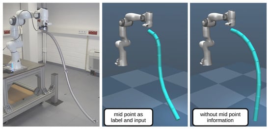
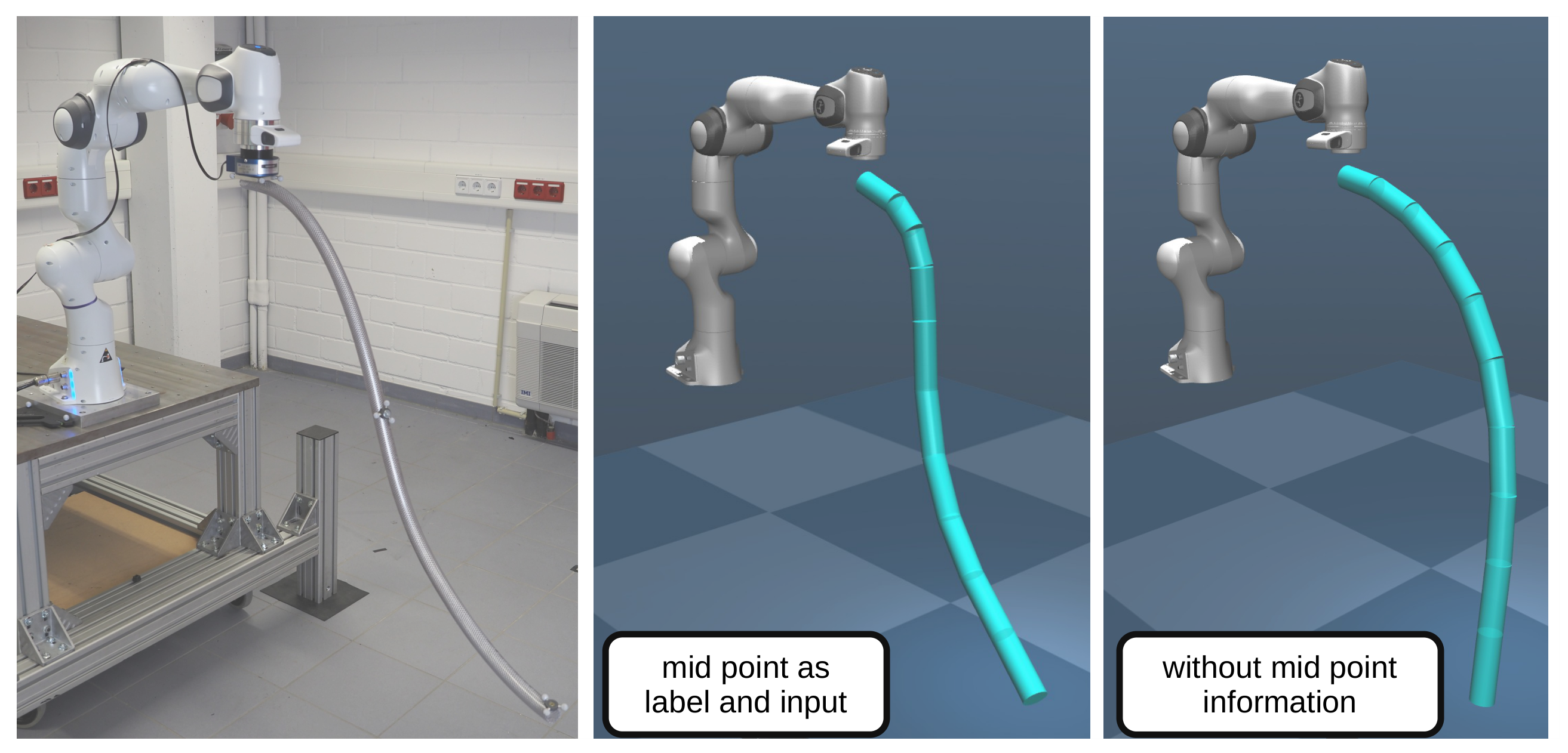
Except for Object A, incorporating mid-point information reduces the distance error between the predicted shape and the mid-position. Adding the mid-position as a training label is sufficient to significantly reduce the error, and this performance is further improved by including it as an encoder input. As expected, the most substantial improvement is observed for Object E, which features a non-monotonic curvature and reducing the mean error from 15 $\mathrm{c}$$\mathrm{m}$ to approximately 1 $\mathrm{c}$$\mathrm{m}$. Without mid-position information, the predicted shape is solely influenced by the tip position and the regularization of the joint position vector, resulting in a monotonically shaped prediction, as depicted in Figure 4.

Figure 4. Comparison of predicted shape of the DLO when using the mid-point information.

With this added information, however, the encoder is forced to predict a shape that respects the mid-position and therefore passes through the mid-point. The additional mid-position information has a bigger influence on the prediction of the tip position and tip velocity.

6. Constrained Model Predictive Control for Dynamic Manipulation

This chapter introduces the approach to achieve constrained model predictive control and provides experiments for evaluating it by introducing hardware and environmental constraints.

6.1. Approach

The DLO system model (8) and OCP (9) only consider the DLO represented as a floating base kinematic chain model. For the control via a robotic manipulator, we augment the state vector in the OCP (9) to include the robot joint state ${\overrightarrow{\mathbf{q}}}_r$ to control a combined robot-DLO system. Assuming a rigid connection between the DLO base and the robot’s end-effector, the base trajectory required by the dynamics model can be obtained directly via forward kinematics. With this formulation, the control input for the combined robot-DLO system becomes the robot joint acceleration $\ddot{\mathbf{q}}$.

To facilitate tracking and constraint evaluation, further information is augmented into the state vector, such as the tip positions, as well as the positions of joint or link frames within the kinematic chain model. This allows constraints to be formulated on discrete points on the kinematic chain model, which is critical for complex maneuvers such as swinging the DLO through a narrow slot.

We solve the resulting OCP using a custom Differential Dynamic Programming (DDP) solver implemented in C++ that employs the iterative Linear Quadratic Regulator (iLQR) variant rather than the full-Newton method and uses analytic derivatives. MPC requires high control frequencies to be effective, so we configure the solver to run for a maximum of three iterations, or when a gradient stopping criterion is met. Since the DDP algorithm does not allow us to formulate constraints natively, constraints are introduced as soft constraints while more detailed information is presented in the evaluation sections.

We keep the general control architecture of [3]. The MPC runs in a high-level controller component and uses the current system state information from the robot DLO system to optimize the robot joint state trajectory to follow a reference. The solved trajectory is then sent to a trajectory buffer, which performs interpolation to sample the trajectory down to the control frequency of the low-level controller. Further, the buffer can perform trajectory blending between consecutive solutions to avoid discontinuous jumps. The final interpolated joint space trajectory is sent as references to a low-level inverse dynamics controller with PD error compensation.

6.2. Evaluation

First, Section 6.2.1 introduces hardware-level limits on joint position, velocity, and acceleration. Subsequently, Section 6.2.2 evaluates the approach under environmental constraints through two scenarios: one restricting the DLO tip position, and a more complex task involving constraints at multiple points along the DLO’s backbone.

6.2.1. Hardware Constraints

To account for hardware, we incorporate soft constraints into the DDP formulation using a relaxed logarithmic barrier method. Concretely, the barrier cost $J_{\mathrm{barrier}}$ (Equation (A2)) is constructed from the relaxed one-sided barrier function $B(·)$ (Equation (A1)) applied to both lower and upper constraint bounds, thereby penalizing violations on either side of the admissible interval. The full formulation is given in Appendix B.1.

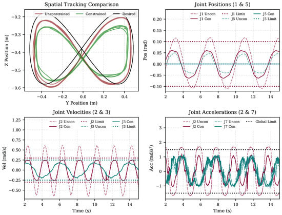
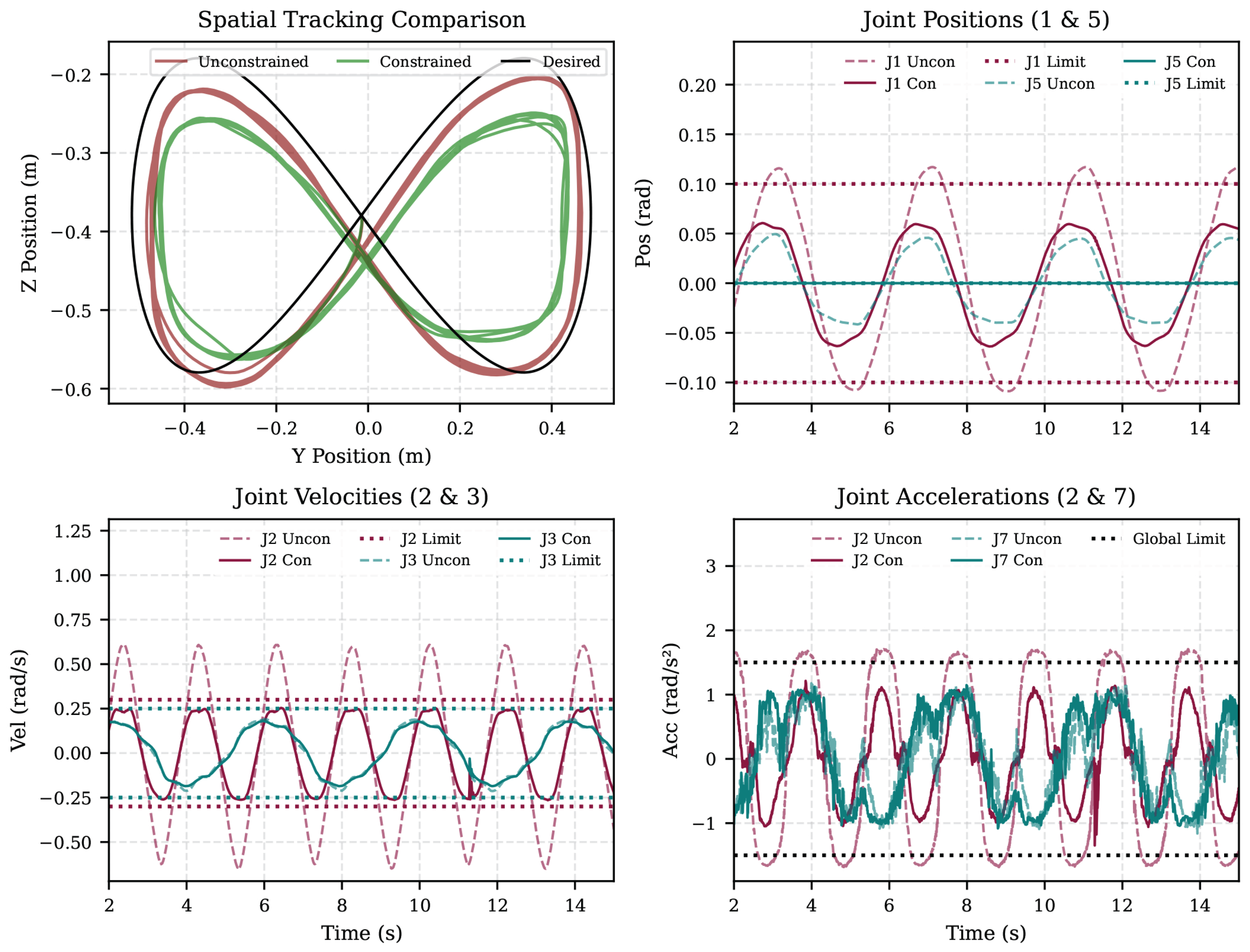
In this experiment, we compare the unconstrained tracking of Object D against a scenario with artificially introduced hardware constraints. Specifically, we restrict the position of joint one to a range of [−0.1, 0.1] $\mathrm{rad}$ and effectively disable joint five by setting its equality constraints to zero $\mathrm{rad}$. Additionally, the velocity of joint two is limited to 0.3 $\mathrm{rad}$ ${\mathrm{s}}^{-1}$, and joint three is limited to 0.25 $\mathrm{rad}$ ${\mathrm{s}}^{-1}$. All joint accelerations are capped at 1.5 $\mathrm{rad}$ ${\mathrm{s}}^{-2}$. Here, we use the Lissajous figure with medium shape completion time, while a more detailed overview over all Figures and speeds is available in Appendix C. As illustrated in Figure 5, the solver successfully respects these constraints, which were otherwise violated in the unconstrained case. Appendix C summarizes the observed soft-constrained violations and the corresponding mean tracking errors for all shapes and speeds. Overall, the results show that the selected penalty weights yield predominantly constraint-compliant behavior and substantially reduce the frequency of violations compared with the unconstrained case. In most settings, violations are eliminated entirely, while residual violations remain only in a few challenging scenarios, most notably for joint 1 during high-speed tracking of the Lissajous trajectory and in isolated acceleration peaks.

Figure 5. Experimental results of tracking the Lissajous figure with artificially defined hardware constraint using Object D.

In general, the soft constraints were tuned conservatively to prioritize practical constraint satisfaction. This conservative tuning, however, can increase the tracking error due to the trade-off between constraint satisfaction and dynamic tracking performance, and because overly large penalty weights may restrict the controller more than necessary.

Similarly, other constraints, such as those acting on the end effector or the DLO base, can be integrated. Theoretically, it is also possible to incorporate the DLO base wrench into the state vector, leveraging the data-driven approximation of the hybrid dynamics, or to impose constraints directly on the DLO joint states. However, in our experiments, these values proved difficult to constrain effectively. They significantly restricted the range of executable motions for dynamic tasks, as they often conflicted with the requirements for high-speed shape tracking, which inherently necessitates larger end-effector wrenches and benefits from natural DLO oscillations.

6.2.2. Environmental Constraints

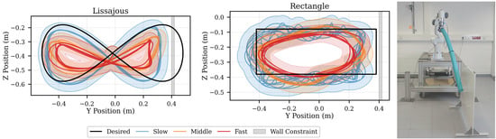
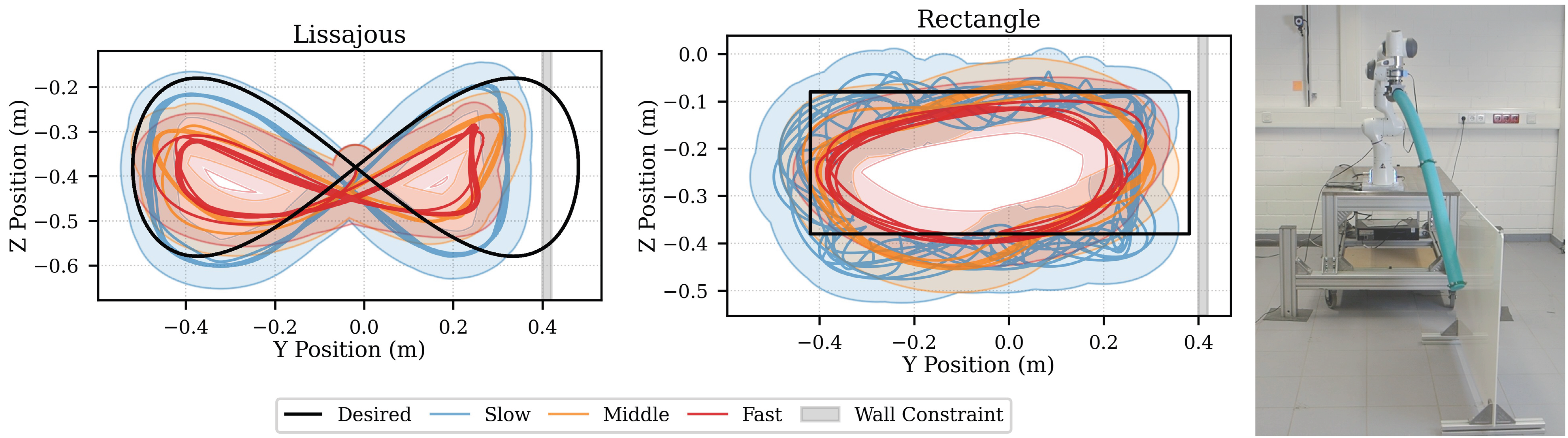
Next, we introduce environmental constraints during the tracking of various shapes. We evaluate the tracking of the Lissajous and rectangular figures across all speeds while placing a wall-like obstacle at y = 0.4 $\mathrm{m}$. This constraint is modeled as a tip-position soft constraint using the same relaxed logarithmic barrier formulation as for the hardware constraints, see Appendix B.1. We validated this approach on physical hardware using Object D. The constraint boundary was set to 0.35 $\mathrm{m}$ to account for the object’s radius and the additional volume of the tracking markers. Figure 6 displays the tip position (solid line) and the space occupied by the tip (envelope). As observed, the system successfully avoids the wall, even when the reference trajectory penetrates the obstacle. Please note that, analogous to the robotic hardware constraints, the tip-related soft constraints were tuned conservatively to prioritize practical constraint satisfaction. In this case, the achieved constraint compliance also depends on the accuracy of the learned dynamics model, while a more detailed analysis of this interaction is beyond the scope of this work.

Figure 6. Tracking the Lissajous and rectangle figure for Object D in the presence of an obstacle.

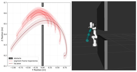
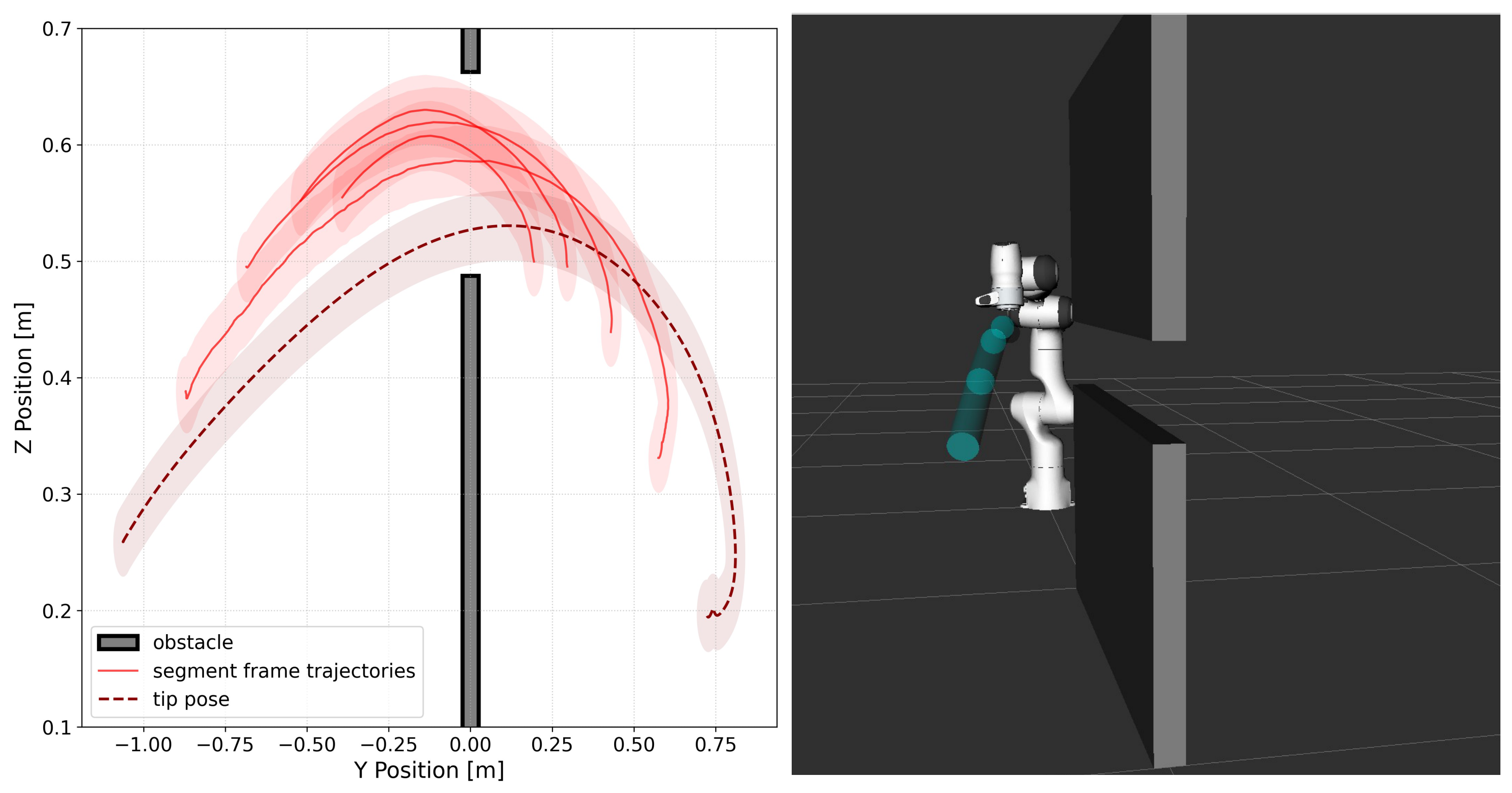
In a separate experiment, we modify the task to command a tip position located on the opposite side of a wall. To reach the target, the robot must maneuver the DLO through a slot between two walls, as illustrated in Figure 7. To enforce collision avoidance, the walls are modeled using continuous artificial potential fields. Specifically, a multivariate Gaussian repulsive term $J_{\mathrm{obs}}$ (Equation (A4)) is centered on each axis-aligned obstacle, yielding a smooth, exponentially decaying penalty around the obstacle whose spatial extent is scaled according to the obstacle dimensions. The exact formulation is given in Appendix B.2. In this setup, the state vector is expanded to include the positions of all joint frames in the kinematic chain model. This ensures that obstacle avoidance is enforced along the entire length of the DLO, rather than just at the tip. In contrast to previous experiments, we adopt an open-loop trajectory optimization approach for this specific task rather than closed-loop MPC. The high-level model predictive controller computes the optimal trajectory once from an initial state, which the low-level controller then tracks. We required this methodological shift because the problem’s increased complexity demands significantly more solver iterations (capped at 30) to achieve convergence to a locally optimal solution.

Figure 7. Simulation results of swinging a DLO object through a slot in a wall.

Initial validation was performed in simulation with a 20 $\mathrm{c}$$\mathrm{m}$ slot. Figure 7 confirms that all considered positions pass through the slot without colliding with the wall.

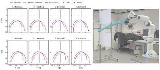
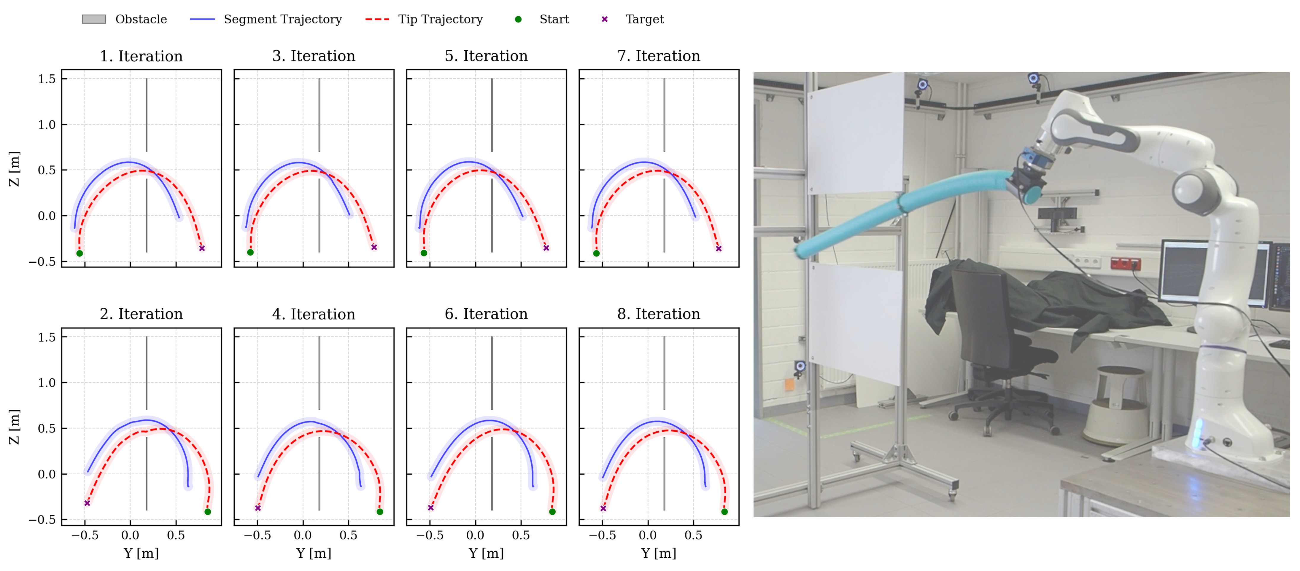
In simulation, the slot-crossing experiment considers obstacle-avoidance constraints along the full DLO backbone. In the following hardware experiment, the physical slot measured 30 $\mathrm{c}$$\mathrm{m}$ in height and 63 $\mathrm{c}$$\mathrm{m}$ in length, and was therefore substantially shorter than the slot considered in simulation. As a result, the slot constraint was applied only to the DLO tip and the terminal joint frame, i.e., to the points that are required to pass through the wall opening. This formulation reduces the constrained set and thereby facilitates the identification of feasible solutions in the hardware experiments. We evaluated the approach with Object D over four cycles, moving the DLO from the left side to the right and back again through the slot. Figure 8 demonstrates that the robot effectively maneuvers the DLO through the opening. However, both the simulation and hardware experiments indicated that this task requires precise tuning of the MPC formulation, especially the tuning of the soft constrained weights, representing the wall obstacles.

Figure 8. Hardware results of swinging Object D repetitively through a slot.

7. Comprehensive Evaluation of the Closed-Loop Control Architecture

Since only a limited number of closely related control approaches are available and these differ in task formulation, assumptions, and implementation details, a strict quantitative comparison with external baselines is not straightforward in the present setting. Accordingly, this section focuses on a comprehensive internal evaluation of the proposed closed-loop control architecture, analyzing performance and computational characteristics across system configurations and object instances.

The overall control architecture consists of different system components, like the model learning of the encoder and dynamic models, state estimation via Kalman filtering and the actual control using the models and state estimations, which all feature a larger number of hyperparameters influencing the final control performance. We begin by evaluating how the number of segments creating the kinematic chain affects the prediction capabilities of the encoders and dynamic networks. Next, we evaluate state estimation via the Kalman filter, comparing it against a baseline, different failure modes and evaluating manual versus hyperparameter search-based filter tuning. Furthermore, we investigate the influence of the number of modeled kinematic chain segments and the size of the neural network modeling its dynamics on controller performance. Finally, we provide an extensive evaluation of the controller across various test objects solving constrained and unconstrained tasks.

7.1. Influence of Number of Segments on Model Learning

The most critical design decision that affects the whole control application architecture is selecting the number of segments that form the kinematic chain representing the DLO. To gain insight into how this discretization affects the prediction capabilities of the encoder and dynamic networks, we conduct the following experiments.

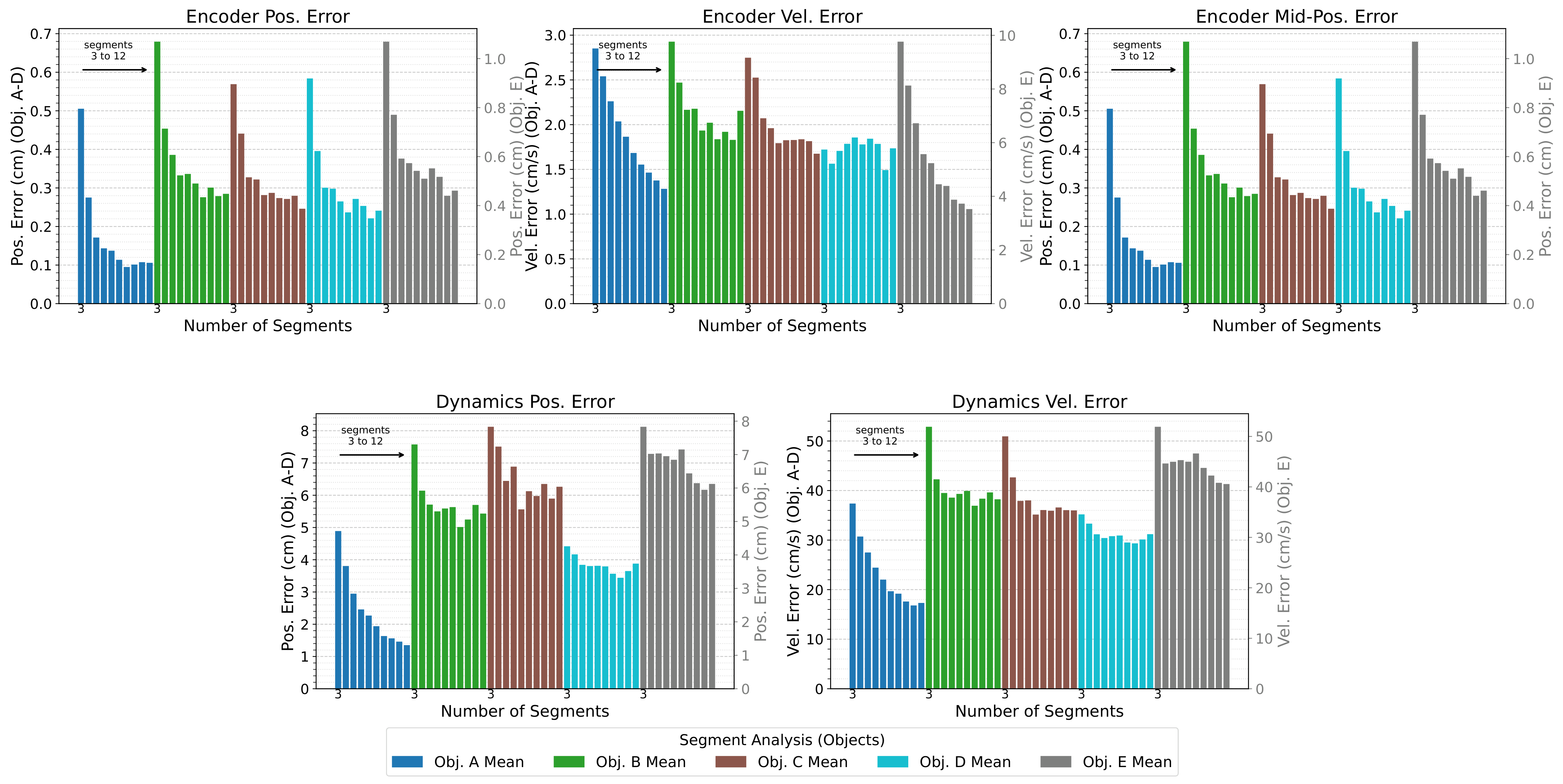
We train various encoder and dynamics models with a varying number of segments. The model architecture remains fixed: two hidden layers with 100 neurons per layer for the encoder, and 128 neurons for the dynamics network. Meanwhile, we vary the number of segments from 3 to 12.

We compare the networks’ ability to predict the tip position, tip velocity, and mid-position across varying numbers of segments in the encoder models. For the dynamics models, we compare the mean tip position and velocity errors over the trained prediction horizon. The results are displayed in Figure 9.

Figure 9. Influence of the number of segments for different DLO objects. The upper row shows the influence on the state estimation, while the lower row shows the influence on the dynamics model.

As the number of segments increases, the encoder results generally show lower prediction errors for the tip position, tip velocity, and mid-position. Using five to six segments significantly reduces the error, while adding more segments beyond this point does not substantially improve the mean prediction accuracy. For the dynamics networks, the mean prediction error is less affected by the number of segments, particularly for configurations with more than five segments. Only Object A exhibits a clear reduction in prediction error with a higher number of segments for both the encoder and dynamics networks.

7.2. State Estimation

This subsection analyzes the practical parameterization and sensitivity of the Kalman filter within the complete control architecture. To gain more insights into the benefits and performance of the Kalman filter, we conducted a comprehensive analysis of the state estimation using the Kalman filter. This section provides evaluations using different objects, failure modes, and hyperparameter selection methods and compares them against a baseline. This evaluation was performed offline using the test datasets collected from the physical hardware.

We assume that the base-wrench-dependent encoders and the Kalman filter’s internal dynamics network remain continuously operational, as they rely on reliably available data. We define four distinct failure modes. In the ’baseline’ scenario, the system operates without failures, providing complete visual information at 240 $\mathrm{Hz}$. In the ’occlusion’ scenario, markers exit the traceable region or become occluded whenever their measured y-position exceeds zero. In the ’short marker loss’ scenario, an unreliable tracking system is simulated: after three seconds into each trajectory, the tip markers are lost during the 0.1–0.2 $\mathrm{s}$ interval of every second, and the mid-marker is lost during the 0.6–0.7 $\mathrm{s}$ interval. In the final ’sensor failure’ scenario, the OptiTrack system ceases operation after 10 $\mathrm{s}$, resulting in a complete loss of tracking information. Whereas the ’occlusion’ and ’short marker loss’ scenarios represent comparatively short interruptions of visual information, the sensor failure scenario leads to a prolonged loss of optical feedback exceeding 14 $\mathrm{s}$, of which 7 $\mathrm{s}$ occur during active motion.

Furthermore, we compare our Kalman filtering (KF) approach against an alternative strategy. One potential solution is to consistently employ the most accurate inverse kinematics solver available. We implement this as a ’relaxed-best policy’ (Best) and evaluate it against our KF method. Under the Best policy, the state prediction from the most accurate inverse kinematics solver is selected at each time step. Because visual information is only acquired at 240 $\mathrm{Hz}$, this policy would inherently cause constant switching between the marker-based and wrench-based solvers. To mitigate this, the best state estimation is held for N time steps. In our implementation, we retain this estimation for five Kalman filter cycles, corresponding to a duration of 5 $\mathrm{m}$$\mathrm{s}$.

For these experiments, we train four distinct encoders. All encoders utilize the DLO base state $\overrightarrow{\mathbf{x}}$ combined with one of the following inputs: (1) the tip state $\overrightarrow{\mathbf{t}}$ and the mid-position $\mathbf{m}$, (2) the tip state $\overrightarrow{\mathbf{t}}$ alone, (3) the mid-position $\mathbf{m}$ alone, or (4) the DLO base wrench ${\mathbf{F}}_b$. Additionally, all objects are modeled using a six-segment kinematic chain.

Further, we compare the performance of the Kalman filter, once with manually tuned filter gains (Manual) and with filter gains obtained via hyperparameter search (Search), which searches for parameters minimizing the prediction error over all scenarios. All the evaluation results are summarized in Table 2. The same set of trajectories and fault scenarios was used for both hyperparameter search and the performance summary in Table 2. Thus, the reported errors may be mildly optimistic and should be interpreted as part of an in-study parameterization analysis rather than as a fully independent held-out evaluation.

Table 2. Comparing the Kalman filter using manual (Manual) and hyperparameter-search-based (Search) filter gains with the Relaxed Best Policy (Best). The table reports the mean ± standard deviation and the maximum error. Hyperparameter search and evaluation were performed on the same trajectory and fault-scenario set.

	Tip Position Error in cm			Mid Position Error in cm			Tip Velocity Error in cm/s
Obj.	Manual	Search	Best	Manual	Search	Best	Manual	Search	Best
Scenario: baseline
A	$\mathbf{0.08}\pm \mathbf{0.1}\left(\mathbf{1}\right)$	$0.09\pm 0.1\left(1\right)$	$0.19\pm 0.2\left(1\right)$	$0.38\pm 0.2\left(1\right)$	$\mathbf{0.29}\pm \mathbf{0.1}\left(\mathbf{1}\right)$	$0.30\pm 0.1\left(1\right)$	$\mathbf{1.37}\pm \mathbf{1.4}\left(\mathbf{9}\right)$	$1.38\pm 1.4\left(10\right)$	$2.58\pm 2.9\left(18\right)$
B	$0.41\pm \mathbf{0.4}\left(\mathbf{4}\right)$	$\mathbf{0.39}\pm 0.5\left(4\right)$	$0.58\pm 0.6\left(4\right)$	$0.50\pm 0.3\left(2\right)$	$\mathbf{0.41}\pm \mathbf{0.3}\left(\mathbf{2}\right)$	$0.43\pm 0.3\left(2\right)$	$\mathbf{3}.\mathbf{45}\pm \mathbf{4}.\mathbf{7}\left(\mathbf{36}\right)$	$3.63\pm 4.9\left(37\right)$	$4.63\pm 5.6\left(40\right)$
C	$0.25\pm \mathbf{0.3}\left(2\right)$	$\mathbf{0.23}\pm 0.3\left(\mathbf{1}\right)$	$0.45\pm 0.5\left(2\right)$	$0.28\pm 0.2\left(1\right)$	$\mathbf{0.20}\pm \mathbf{0.2}\left(\mathbf{1}\right)$	$0.25\pm 0.2\left(1\right)$	$\mathbf{2.13}\pm \mathbf{2.4}\left(\mathbf{13}\right)$	$2.20\pm 2.6\left(14\right)$	$3.67\pm 4.3\left(20\right)$
D	$0.17\pm 0.2\left(1\right)$	$\mathbf{0.17}\pm \mathbf{0.2}\left(\mathbf{1}\right)$	$0.34\pm 0.4\left(2\right)$	$0.32\pm 0.1\left(1\right)$	$\mathbf{0.32}\pm \mathbf{0.1}\left(\mathbf{1}\right)$	$0.35\pm 0.1\left(1\right)$	$\mathbf{1.57}\pm \mathbf{2.0}\left(\mathbf{14}\right)$	$1.81\pm 2.3\left(18\right)$	$3.14\pm 3.8\left(20\right)$
E	$0.28\pm 0.2\left(2\right)$	$\mathbf{0.28}\pm \mathbf{0.2}\left(\mathbf{2}\right)$	$0.41\pm 0.4\left(2\right)$	$0.74\pm 0.2\left(2\right)$	$\mathbf{0.69}\pm 0.2\left(1\right)$	$0.70\pm \mathbf{0.2}\left(\mathbf{1}\right)$	$\mathbf{1.87}\pm \mathbf{2}.\mathbf{3}\left(\mathbf{15}\right)$	$2.21\pm 2.7\left(18\right)$	$2.78\pm 3.1\left(17\right)$
Scenario: occlusion
A	$1.01\pm \mathbf{0.8}\left(\mathbf{5}\right)$	$\mathbf{0.99}\pm 0.9\left(5\right)$	$1.19\pm 1.3\left(8\right)$	$0.69\pm 0.5\left(3\right)$	$\mathbf{0.60}\pm \mathbf{0.4}\left(\mathbf{3}\right)$	$0.64\pm 0.5\left(4\right)$	$8.95\pm 10.9\left(68\right)$	$\mathbf{7.02}\pm \mathbf{6.5}\left(\mathbf{37}\right)$	$8.15\pm 7.3\left(47\right)$
B	$2.60\pm 3.2\left(23\right)$	$\mathbf{2.18}\pm \mathbf{2.1}\left(\mathbf{14}\right)$	$2.41\pm 2.3\left(14\right)$	$1.51\pm 1.7\left(12\right)$	$1.16\pm 1.0\left(6\right)$	$\mathbf{1.08}\pm \mathbf{0.8}\left(\mathbf{5}\right)$	$18.68\pm 26.5\left(174\right)$	$\mathbf{16.71}\pm \mathbf{19.9}\left(\mathbf{134}\right)$	$20.02\pm 23.1\left(139\right)$
C	$\mathbf{2.05}\pm 2.3\left(13\right)$	$2.08\pm \mathbf{2.1}\left(\mathbf{11}\right)$	$2.36\pm 2.3\left(11\right)$	$1.37\pm 1.6\left(9\right)$	$0.98\pm 0.9\left(4\right)$	$\mathbf{0.94}\pm \mathbf{0.8}\left(\mathbf{4}\right)$	$13.89\pm 14.8\left(81\right)$	$\mathbf{13.43}\pm \mathbf{13.6}\left(\mathbf{64}\right)$	$16.42\pm 16.3\left(79\right)$
D	$1.35\pm 1.4\left(8\right)$	$\mathbf{1.30}\pm \mathbf{1.3}\left(\mathbf{8}\right)$	$1.42\pm 1.4\left(9\right)$	$0.99\pm 1.1\left(6\right)$	$0.80\pm 0.7\left(4\right)$	$\mathbf{0.65}\pm \mathbf{0.5}\left(\mathbf{3}\right)$	$9.24\pm 11.1\left(65\right)$	$\mathbf{8.69}\pm \mathbf{10.4}\left(\mathbf{59}\right)$	$9.45\pm 12.4\left(65\right)$
E	$\mathbf{1.36}\pm \mathbf{1.8}\left(\mathbf{11}\right)$	$1.40\pm 1.8\left(11\right)$	$1.68\pm 2.0\left(12\right)$	$1.24\pm 0.9\left(6\right)$	$1.08\pm 0.7\left(5\right)$	$\mathbf{1.00}\pm \mathbf{0.6}\left(\mathbf{4}\right)$	$\mathbf{9.87}\pm \mathbf{11.9}\left(\mathbf{69}\right)$	$9.97\pm 12.1\left(72\right)$	$11.79\pm 14.2\left(91\right)$
Scenario: sensor failure
A	$1.18\pm \mathbf{0.8}\left(\mathbf{5}\right)$	$\mathbf{1.14}\pm 1.0\left(6\right)$	$1.28\pm 1.4\left(9\right)$	$0.69\pm 0.5\left(3\right)$	$\mathbf{0.63}\pm \mathbf{0.4}\left(\mathbf{3}\right)$	$0.68\pm 0.6\left(4\right)$	$7.72\pm 10.1\left(65\right)$	$\mathbf{7.11}\pm \mathbf{6.7}\left(\mathbf{43}\right)$	$8.76\pm 7.7\left(51\right)$
B	$3.78\pm 4.1\left(27\right)$	$\mathbf{2.78}\pm \mathbf{2.2}\left(\mathbf{13}\right)$	$2.83\pm 2.3\left(14\right)$	$1.82\pm 1.7\left(10\right)$	$1.36\pm 1.1\left(6\right)$	$\mathbf{1.23}\pm \mathbf{0.9}\left(\mathbf{6}\right)$	$22.14\pm 29.0\left(182\right)$	$\mathbf{18.53}\pm \mathbf{20.0}\left(\mathbf{107}\right)$	$21.23\pm 23.2\left(125\right)$
C	$2.61\pm 2.8\left(17\right)$	$\mathbf{2.20}\pm \mathbf{2.1}\left(\mathbf{11}\right)$	$2.25\pm 2.2\left(12\right)$	$1.52\pm 1.9\left(11\right)$	$0.98\pm 1.0\left(5\right)$	$\mathbf{0.87}\pm \mathbf{0.8}\left(\mathbf{4}\right)$	$13.60\pm 17.0\left(100\right)$	$\mathbf{12.06}\pm \mathbf{14.0}\left(\mathbf{70}\right)$	$13.13\pm 15.7\left(77\right)$
D	$1.70\pm 1.6\left(\mathbf{8}\right)$	$\mathbf{1.57}\pm \mathbf{1.4}\left(8\right)$	$1.57\pm 1.4\left(9\right)$	$1.17\pm 1.2\left(6\right)$	$0.91\pm 0.8\left(4\right)$	$\mathbf{0.69}\pm \mathbf{0.5}\left(\mathbf{3}\right)$	$10.92\pm 12.2\left(65\right)$	$\mathbf{10.10}\pm \mathbf{11.3}\left(\mathbf{58}\right)$	$10.19\pm 12.6\left(65\right)$
E	$1.65\pm 1.8\left(12\right)$	$\mathbf{1.57}\pm \mathbf{1.6}\left(\mathbf{11}\right)$	$1.63\pm 1.7\left(11\right)$	$1.27\pm 0.8\left(6\right)$	$1.10\pm 0.6\left(4\right)$	$\mathbf{1.00}\pm \mathbf{0.5}\left(\mathbf{4}\right)$	$8.49\pm 10.8\left(67\right)$	$\mathbf{8.13}\pm \mathbf{10.3}\left(\mathbf{64}\right)$	$8.53\pm 11.0\left(64\right)$
Scenario: short marker loss
A	$\mathbf{0.31}\pm \mathbf{0.4}\left(\mathbf{2}\right)$	$0.36\pm 0.4\left(3\right)$	$0.54\pm 0.6\left(3\right)$	$0.50\pm 0.3\left(2\right)$	$\mathbf{0.48}\pm \mathbf{0.3}\left(\mathbf{2}\right)$	$0.48\pm 0.3\left(2\right)$	$6.12\pm 7.8\left(46\right)$	$\mathbf{4.48}\pm \mathbf{5.0}\left(\mathbf{28}\right)$	$5.69\pm 6.0\left(31\right)$
B	$\mathbf{1.12}\pm \mathbf{1.2}\left(\mathbf{10}\right)$	$1.44\pm 1.6\left(12\right)$	$1.53\pm 1.7\left(12\right)$	$\mathbf{0.71}\pm \mathbf{0.6}\left(\mathbf{4}\right)$	$0.73\pm 0.6\left(4\right)$	$0.75\pm 0.6\left(4\right)$	$\mathbf{10.17}\pm \mathbf{14.8}\left(\mathbf{108}\right)$	$15.09\pm 22.0\left(160\right)$	$15.65\pm 21.6\left(158\right)$
C	$\mathbf{0.69}\pm \mathbf{0.8}\left(\mathbf{5}\right)$	$0.75\pm 0.9\left(6\right)$	$1.05\pm 1.1\left(7\right)$	$0.45\pm 0.4\left(2\right)$	$\mathbf{0.41}\pm \mathbf{0.4}\left(\mathbf{2}\right)$	$0.44\pm 0.4\left(2\right)$	$\mathbf{6.20}\pm \mathbf{7.7}\left(\mathbf{44}\right)$	$6.81\pm 9.0\left(53\right)$	$9.41\pm 12.0\left(71\right)$
D	$\mathbf{0.32}\pm \mathbf{0.4}\left(\mathbf{3}\right)$	$0.33\pm 0.4\left(3\right)$	$0.57\pm 0.6\left(4\right)$	$\mathbf{0.39}\pm \mathbf{0.2}\left(1\right)$	$0.40\pm 0.2\left(\mathbf{1}\right)$	$0.40\pm 0.2\left(2\right)$	$4.09\pm 5.1\left(35\right)$	$\mathbf{4.04}\pm \mathbf{4.9}\left(\mathbf{34}\right)$	$5.88\pm 7.2\left(50\right)$
E	$0.67\pm 0.8\left(\mathbf{5}\right)$	$\mathbf{0.64}\pm \mathbf{0.7}\left(5\right)$	$0.95\pm 1.0\left(6\right)$	$0.83\pm 0.3\left(\mathbf{2}\right)$	$\mathbf{0.82}\pm \mathbf{0.3}\left(2\right)$	$0.85\pm 0.3\left(2\right)$	$\mathbf{4.72}\pm \mathbf{6.1}\left(\mathbf{47}\right)$	$5.01\pm 6.7\left(49\right)$	$7.20\pm 9.7\left(64\right)$

For the failure modes, estimation errors are reported exclusively for the duration of the failure, as performance returns to baseline levels once the failure resolves. For comparison, Table 3 presents the performance of the individual encoders.

Table 3. Prediction performance of data-driven inverse kinematics solvers. The table reports the mean ± standard deviation and the maximum error.

Object	Encoder Input	Tip Position Error in cm	Mid Position Error in cm	Tip Velocity Error in cm
A	tip + mid	0.1 ± 0.1 (1)	0.3 ± 0.1 (1)	1.3 ± 1.3 (9)
	tip	0.1 ± 0.2 (1)	0.5 ± 0.4 (2)	1.5 ± 1.6 (10)
	mid	0.7 ± 0.7 (4)	0.4 ± 0.2 (1)	7.5 ± 6.6 (33)
	wrench	1.4 ± 1.5 (9)	0.7 ± 0.7 (4)	9.8 ± 8.7 (56)
B	tip + mid	0.4 ± 0.5 (4)	0.4 ± 0.3 (2)	3.7 ± 4.9 (39)
	tip	0.7 ± 0.7 (6)	0.7 ± 0.5 (4)	5.0 ± 6.8 (51)
	mid	2.1 ± 1.9 (14)	0.6 ± 0.6 (5)	23.3 ± 28.7 (177)
	wrench	2.8 ± 2.2 (14)	1.2 ± 0.9 (5)	22.2 ± 22.8 (132)
C	tip + mid	0.2 ± 0.3 (1)	0.2 ± 0.2 (1)	2.2 ± 2.6 (14)
	tip	0.4 ± 0.4 (2)	0.4 ± 0.3 (2)	2.8 ± 3.0 (16)
	mid	1.3 ± 1.2 (7)	0.4 ± 0.4 (3)	11.6 ± 13.2 (76)
	wrench	2.6 ± 2.3 (12)	1.0 ± 0.9 (4)	16.1 ± 17.0 (82)
D	tip + mid	0.2 ± 0.2 (1)	0.3 ± 0.1 (1)	1.8 ± 1.9 (14)
	tip	0.2 ± 0.3 (2)	0.3 ± 0.1 (1)	2.1 ± 2.7 (20)
	mid	0.4 ± 0.5 (3)	0.3 ± 0.2 (2)	6.2 ± 7.5 (53)
	wrench	1.8 ± 1.6 (9)	0.8 ± 0.6 (3)	12.6 ± 14.4 (72)
E	tip + mid	0.3 ± 0.2 (2)	0.7 ± 0.2 (1)	2.0 ± 2.3 (16)
	tip	0.4 ± 0.4 (3)	0.9 ± 0.3 (2)	2.5 ± 3.4 (21)
	mid	1.2 ± 1.1 (7)	0.8 ± 0.3 (2)	9.1 ± 11.8 (75)
	wrench	1.8 ± 2.0 (12)	1.0 ± 0.6 (5)	10.5 ± 13.0 (84)

Across all scenarios and objects, the Kalman filter approach demonstrates slightly improved performance compared to the relaxed-best policy, particularly regarding tip velocity prediction. However, the prediction of the mid-position is not consistently superior using the Kalman filter, although the performance difference is marginal. This discrepancy occurs because the prediction of tip quantities was weighted more heavily than the mid-position during the training process and hyperparameter search for the Kalman filter. The manually tuned filter gains tend to perform similarly to the gains obtained via hyperparameter search in scenarios with small tracking errors. When more failure cases occur in the tracking system, as emulated by the occlusion and sensor-failure scenarios, the tracking performance of the manually obtained filter gains is worse, but still better than the Best policy.

The Kalman filter introduces only minor improvements compared to the Best policy. These gains are beneficial but appear not to be critical for the control application under reliable tracking conditions. Nevertheless, the Kalman filter remains attractive in our architecture because it enables principled recursive fusion, provides an explicit uncertainty representation through the covariance, and allows a straightforward incorporation of the learned dynamics model into the state-estimation process. This comes at the cost of additional tuning effort for the filter covariance parameters, which represents the main practical overhead compared to simpler fusion strategies.

7.3. Study: Hyperparameter Influence on Control Approach

While the two previous investigations focused solely on individual components of the control architecture, all components collectively influence final task performance. Specifically, the number of segments and the size of the dynamics network are critical for the computation times and controller performances. Therefore, before conducting the primary control experiments, we present a preliminary study to evaluate how these parameters influence the performance and computational requirements of the MPC. We simulate a tracking task in which the robot follows ten Lissajous figures using the DLO tip. Encoder and dynamics models are trained using 4, 8, and 12 segments. Additionally, we evaluate dynamics models utilizing two hidden layers with 32, 128, or 256 neurons per layer. All experiments are conducted in simulation on a computing hardware equipped with an AMD Ryzen 9 9950X3D.

We evaluate the tracking performance by evaluating the mean error of the tip from the reference and only consider the error in the y–z plane. Furthermore, we measure the computation time for a single DDP iteration and the time for evaluating the robot-DLO dynamical system with the augmented tip state by solving Equation (8) and applying an explicit Euler integration step to map to the next state, a process denoted as the forward step. Because this system must be linearized within the DDP solvers’ backward step, we record the time required to differentiate the system. Since the MLP approximating the dynamical system is a critical component, we additionally measure the time taken for its forward prediction and network differentiation. Table 4 presents the results of these experiments.

Table 4. Parameter analysis: Influence on the tracking performance and computation.

Number Segments	MLP Neurons per Layer	Tracking Accuracy in cm	Duration DDP Iteration in ms	DLO Dynamics Forward in μs	DLO Dynamics Differentiation in μs	MLP: Forward in μs	MLP: Differentiation in μs
4	32	2.95 ± 1.49 (9.5)	6.07	1.01	8.91	0.61	2.02
	128	2.93 ± 0.82 (5.5)	7.39	3.13	25.15	3.04	15.11
	256	3.20 ± 0.9 (5.6)	8.66	7.05	32.06	6.53	18.68
8	32	6.20 ± 4.5 (19.1)	10.18	1.02	15.3	0.65	4.01
	128	2.80 ± 0.9 (5.4)	11.56	4.01	30.24	3.28	16.15
	256	3.00 ± 1.3 (6.2)	13.4	7.97	209.14	6.97	207.744
12	32	8.74 ± 5.9 (21.1)	16.69	2.01	24.27	0.69	6.03
	128	3.10 ± 1.5 (7.7)	17.88	4.09	78.28	3.50	56.44
	256	2.44 ± 0.9 (4.9)	20.27	8.23	341.45	7.49	338.96

The table reveals several interesting phenomena. First, the optimal performance is achieved using 12 segments and the largest neural network. However, maximizing the network size does not consistently guarantee the best tracking performance. Tracking accuracy is governed by both the number of segments and the network size, which concurrently affect computation times. The state dimension changed by the number of segments has the most significant influence on the computation time per DDP iteration, whereas the network size has only a minor impact.

7.4. Unconstrained MPC

For the controller performance, we use, in total, six different objects and two simulation objects to evaluate how the object characteristics influence the tracking performance. For the control experiments, all objects are modeled as a floating-base kinematic chain with six segments. As a proof of concept, Object F is modeled with only three segments, as it is highly rigid and exhibits minor vibrations in only one direction, and the solver runs 5 DDP iterations for this object.

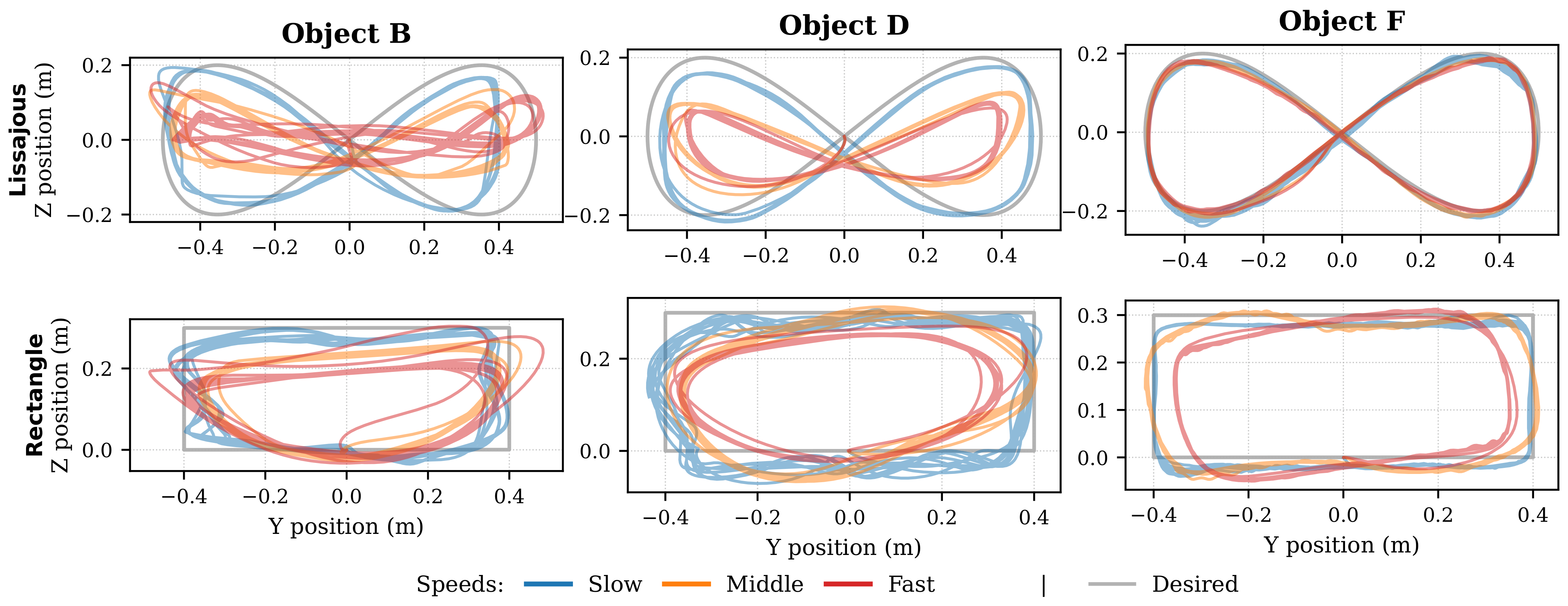
The MPC hyperparameters are tuned to track all shapes and speeds using a single set of parameters per object. The parameters of the OCP in (9) are initialized heuristically using Bryson’s rule and then manually tuned to achieve good task performance and ensure smooth and stable robot motions across all reference speeds. The numerical tracking results are presented in Table 5, while Figure 10 visualizes the tracking performance for the Lissajous and rectangular shapes across select objects.

Table 5. Tracking performance across different objects and shape speeds. The table reports the mean ± standard deviation and the maximum error.

Object	Speed	Tracking Error in cm	Solver Iterations	Solver Time per Iteration in ms
Simulation  Stiff	Slow	$2.3\pm 0.4\left(3.8\right)$	1.8	6.6
	Middle	$2.6\pm 0.9\left(7.3\right)$	2.0	5.9
	Fast	$3.0\pm 1.3\left(10.3\right)$	2.0	5.0
Simulation  Soft	Slow	$1.6\pm 0.7\left(5.0\right)$	1.9	5.7
	Middle	$2.6\pm 1.4\left(9.8\right)$	2.0	5.4
	Fast	$3.8\pm 2.0\left(14.2\right)$	2.2	4.9
Object A	Slow	$10.2\pm 1.9\left(14.5\right)$	2.3	4.8
	Middle	$10.1\pm 2.8\left(16.2\right)$	2.3	4.9
	Fast	$10.2\pm 3.5\left(19.3\right)$	2.3	4.8
Object B	Slow	$5.8\pm 2.9\left(15.1\right)$	2.6	4.9
	Middle	$8.2\pm 3.6\left(18.4\right)$	2.8	5.0
	Fast	$10.4\pm 4.8\left(24.4\right)$	2.9	5.1
Object C	Slow	$11.4\pm 4.7\left(27.2\right)$	2.9	5.2
	Middle	$10.1\pm 3.6\left(26.8\right)$	2.9	5.2
	Fast	$12.8\pm 5.6\left(32.0\right)$	3.0	5.5
Object D	Slow	$4.0\pm 1.5\left(9.6\right)$	2.0	4.7
	Middle	$7.0\pm 2.5\left(15.3\right)$	2.0	4.7
	Fast	$8.5\pm 2.8\left(16.9\right)$	2.1	4.8
Object E	Slow	$10.4\pm 5.7\left(27.1\right)$	3.0	5.7
	Middle	$15.8\pm 7.5\left(67.8\right)$	3.0	6.0
Object F	Slow	$2.3\pm 1.0\left(5.4\right)$	4.0	3.0
	Middle	$2.6\pm 1.1\left(6.4\right)$	4.8	3.5
	Fast	$3.7\pm 1.7\left(13.3\right)$	4.9	3.6

Figure 10. Results of tracking the Lissajous and rectangular shape with different speeds for different objects.

Object E could only be controlled at slow and medium speeds, as the fast speed exceeded the robot’s hardware limits. Overall, both the simulation and Object F demonstrate good tracking performance. However, the deformable objects exhibit significantly poorer performance, even during slow trajectories. Only Objects B and D achieved tracking errors below 10 $\mathrm{c}$$\mathrm{m}$ for the slow and medium speeds. On the real hardware, the solver averages 4.7 to 6.0 $\mathrm{m}$$\mathrm{s}$ per DDP iteration, typically requiring 2–3 iterations. This corresponds to a control frequency of approximately 55.5–106 $\mathrm{Hz}$.

The tracking experiments highlight the remaining challenges in controlling DLOs. Dynamic DLOs constitute highly underactuated systems with many DoF and strongly nonlinear deformation behavior, which makes accurate modeling difficult even when using data-driven black-box approaches. In addition, closed-loop tracking of dynamic endpoint motions imposes strict real-time constraints. To maintain a sufficiently high control rate, the present implementation relies on a reduced-order representation (floating-base kinematic chain), simplified data-driven dynamics, and limited solver iterations per control cycle. These choices improve computational efficiency, but reduce model fidelity and optimization quality. Consequently, the observed tracking performance reflects not only the intrinsic physical difficulty of the task, but also a practical trade-off between accuracy and real-time responsiveness. This trade-off is illustrated by the comparatively better results for Object F. In simulation, the object dynamics are generated from a relatively simple kinematic-chain model, which is well aligned with the reduced representation used by the controller. On hardware, Object F is also comparatively stiff and physically simpler than the other objects. These conditions reduce deformation complexity and make tracking easier. In contrast, for the more deformable objects (B–E), tracking performance is limited by the combination of underactuation, complex deformation dynamics, and the model and solver simplifications required for real-time control. Using a more expressive dynamics model or a larger solver budget could improve prediction accuracy, but would also increase latency and reduce control frequency. For fast dynamic motions, this may offset some of the potential accuracy gains. A more systematic analysis of this trade-off is an important direction for future work.

Another potential improvement involves tuning the MPC specifically for a given shape and speed. However, applying these specialized hyperparameters to different shapes or speeds can induce instabilities, for example, if the controller reacts too aggressively to deviations or material oscillations. This was particularly evident when transitioning from fast to slow motions. Fast motions necessitate high accelerations; however, allowing such high accelerations during slow motions often causes the MPC to overcompensate for errors, injecting high-frequency inputs that trigger resonance within the DLO system.

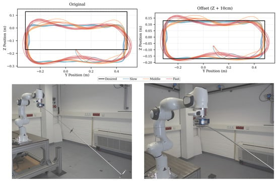
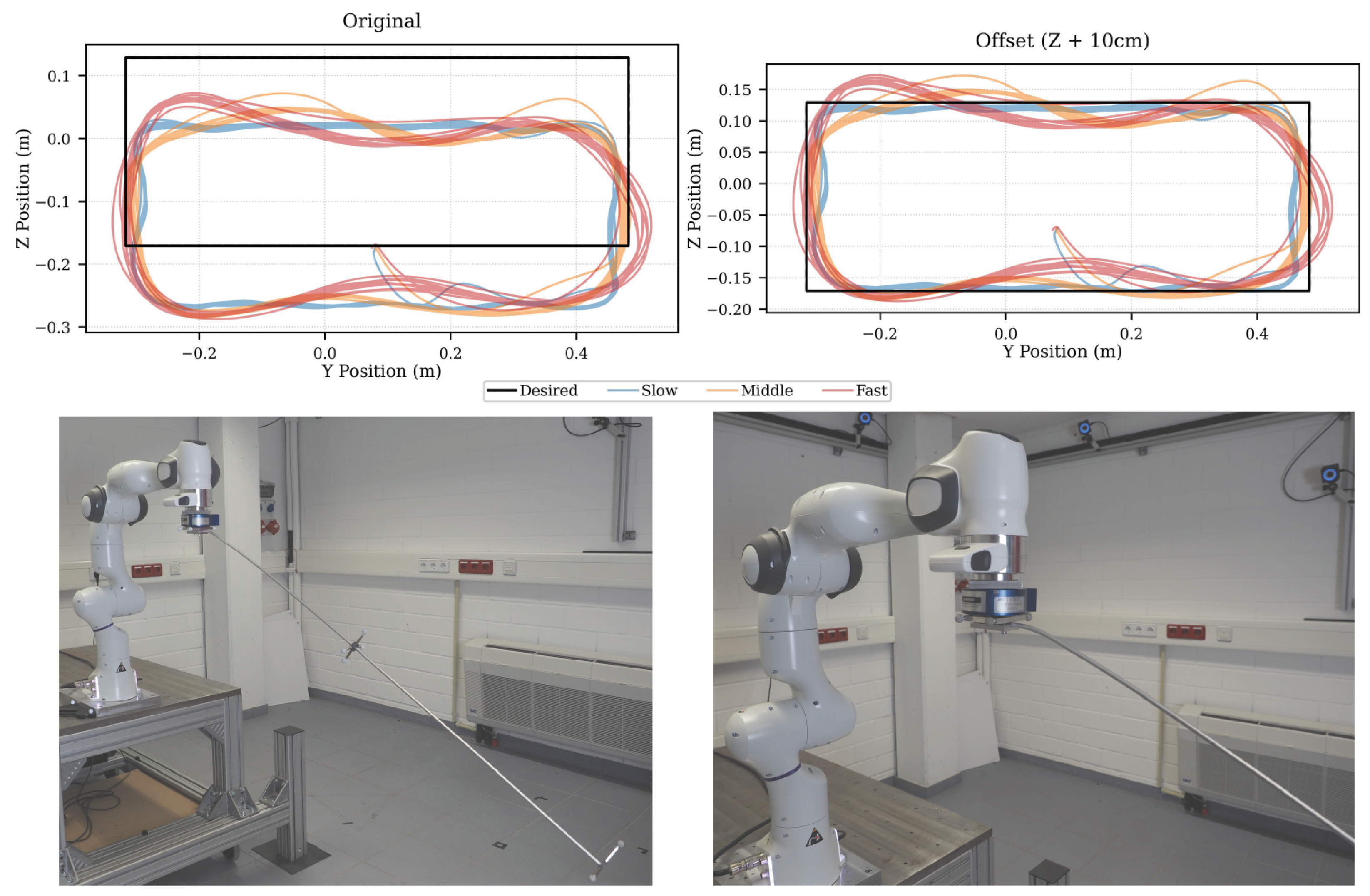
Object A exhibits a large tracking error despite its relative stiffness. This is attributed to plastic deformations that occurred during data collection and hyperparameter tuning. Initially straight, Object A developed a bend near the grasping location, as illustrated in Figure 11.

Figure 11. Tracking results Object A, once with real data on the left side and one with an added offset of 10 $\mathrm{c}$$\mathrm{m}$ in the Z-direction. The lower images show the bending of Object A compared to the starting configuration in Figure 3.

This distribution shift resulted in a tracking error of approximately 10 $\mathrm{c}$$\mathrm{m}$, primarily in the Z-direction. If the actual trajectory is virtually shifted by the mean tracking error in the +Z direction, the average errors drop from around 10 $\mathrm{c}$$\mathrm{m}$ to 2.3 cm, 3.9 cm and 5.4 $\mathrm{c}$$\mathrm{m}$. This indicates that the distribution shift caused by plastic deformation led to the shape being tracked with a consistent offset. In practice, plastic and viscoplastic deformations frequently occur in DLOs. Currently, there is no mechanism within these data-driven models to account for post-training distribution shifts. Therefore, an important avenue for future research is to investigate how these shifts affect the performance of the DDIK, state estimation, and dynamic models, as well as to identify suitable measures to mitigate them.

8. Conclusions

In this paper, we introduced several advancements for manipulating DLOs in highly dynamic situations, beginning with improvements to state estimation. We proposed incorporating additional marker locations on the DLO to enable more accurate state estimation and shape matching. We demonstrated that a single additional via point significantly improves shape prediction for non-monotonically curved objects, while already including the marker position as a training label is sufficient to improve the shape matching.

Building on these estimation improvements, we advanced the control framework by incorporating hardware and environmental constraints into the MPC formulation via soft constraints. We demonstrated the validity of this approach through hardware experiments that successfully constrained robot joint positions, velocities, and accelerations, while simultaneously handling environmental challenges such as obstacle avoidance and swinging a DLO through a narrow slot, while the latter challenging slot passing task was achieved in open-loop fashion.

Finally, we presented an extensive real-world evaluation of our overall control application architecture using five distinct objects to analyze interacting parameters, hyperparameters, and system challenges. We investigated how the number of segments in the floating-base kinematic chain influences the prediction capabilities of data-driven inverse kinematics and the learning of hybrid dynamics approximations. Although all objects exhibit better prediction capabilities with more modeled DoF, we found that five to six segments provide a sufficiently accurate approximation, while increasing this number yields diminishing returns.

Further, we comprehensively analyzed state estimation using our Kalman filter approach across various failure modes, comparing it against a “relaxed best policy” baseline and different hyperparameter selection methods. Although the Kalman filter improves performance, these gains are not critical when an already reliable tracking system is available. Future work should extend this evaluation toward broader benchmarking against external control approaches under harmonized experimental conditions.

The inherent dynamics of deformable objects heavily influence system performance, making the accurate control of underactuated DLOs a fundamental challenge. During fast motions, tracking performance for highly soft objects degrades significantly, as the requisite large, rapid end-effector movements can induce instability. This fragility is exacerbated by distribution shifts, such as the plastic deformations observed in Object A. Because current data-driven models lack mechanisms to handle these post-training physical changes, developing robust strategies to mitigate their impact on state estimation and dynamic modeling remains a critical priority for future research. Ultimately, the successful deployment of this architecture relies on precise, task-specific hyperparameter tuning, particularly regarding the number of segments, the dynamics network size, and the OCP cost function parameters.

Appendix B.1. Relaxed Logarithmic Barrier Method for Two-Side Bounded Constraints

For a constrained state or control component ${\xi }_i\in \{x_k\left[i\right],u_k\left[i\right]\}$ with bounds ${\xi }_i^{min}\le {\xi }_i\le {\xi }_i^{max}$, we define the distances to the bounds $d_i^{+}={\xi }_i^{max}-{\xi }_i$ and $d_i^{-}={\xi }_i-{\xi }_i^{min}$, and penalize each with the relaxed log-barrier

$$B(d;w,\delta )=\left\{\begin{array}{cc}-wln\left(d\right),\hfill & d>\delta \hfill \\ \frac{1}{2}k{d}^2+bd+c,\hfill & d\le \delta ,\hfill \end{array}\right.k=\frac{w}{{\delta }^2},b=-\frac{2w}{\delta },c=w\left(\frac{3}{2}-ln\delta \right),$$

(A1)

where the quadratic branch is matched in value, slope and curvature to the logarithmic branch at $d=\delta$, keeping B finite and $C^2$ even under a transient constraint violation ($d\le 0$). The total barrier cost is

$$J_{\mathrm{barrier}}\left(\xi \right)=\sum _{i\in \mathcal{I}}\left[B(d_i^{+};w_i,{\delta }_i)+B(d_i^{-};w_i,{\delta }_i)\right].$$

(A2)

Appendix B.2. Gaussian Penalty for Obstacle Avoidance

The two walls forming the passing slot are modeled as axis-aligned boxes and enforced as soft constraints through an anisotropic Gaussian repulsive potential, evaluated at every tracked body point p of the DLO (tip and segment frames) with position ${\zeta }_p\in {\mathbb{R}}^3$ given by the corresponding entries of the state vector. For an obstacle with center $c\in {\mathbb{R}}^3$ and full edge lengths $D\in {\mathbb{R}}^3$ along each axis (additionally inflated by twice a safety radius r, i.e., $D_j+=2r$, to account for the DLO thickness), the per-axis standard deviation is

$${\sigma }_j={\displaystyle \frac{D_j}{s}},j\in \{1,2,3\},$$

(A3)

where $s>0$ is a sharpness factor controlling how steeply the potential decays away from the obstacle surface. The resulting cost is a diagonal Gaussian centered at c,

$$J_{\mathrm{obs}}\left({\zeta }_p\right)=wexp\left(-\frac{1}{2}{\displaystyle \sum _{j=1}^3}{\displaystyle \frac{{({\zeta }_{p,j}-c_j)}^2}{{\sigma }_j^2}}\right),$$

(A4)

with weight $w>0$, maximal at the obstacle center and decaying smoothly and exponentially with distance, anisotropically scaled by the (inflated) obstacle’s dimensions. As a smooth $C^{\infty }$ function, it admits closed-form gradients and Hessians and integrates directly into the DDP backward pass.

The total collision-avoidance cost sums this potential over all monitored body points $\mathcal{P}$ and all obstacles $\mathcal{O}$ (the two walls bounding the slot):

$$J_{\mathrm{obs},\mathrm{total}}=\sum _{p\in \mathcal{P}}\sum _{o\in \mathcal{O}}{J}_{\mathrm{obs}}^{\left(o\right)}\left({\zeta }_p\right).$$

(A5)

In the passing-task experiment, $\mathcal{P}$ contains the DLO tip and five segment frames, and $w,s$ are shared across obstacles, so the effective gap width is governed by the wall geometry (inflated by r) and s.

References

- Sanchez, J.; Corrales, J.-A.; Bouzgarrou, B.-C.; Mezouar, Y. Robotic manipulation and sensing of deformable objects in domestic and industrial applications: A survey. Int. J. Robot. Res. 2018, 37, 688–716. [Google Scholar] [CrossRef] [Scilit]
- Arriola-Rios, V.E.; Guler, P.; Ficuciello, F.; Kragic, D.; Siciliano, B.; Wyatt, J.L. Modeling of Deformable Objects for Robotic Manipulation: A Tutorial and Review. Front. Robot. AI 2020, 7, 82. [Google Scholar] [CrossRef] [Scilit] [PubMed]
- Klankers, M.K.; Steil, J.J. Closed-Loop Trajectory Optimization of Deformable Linear Objects for Dynamic Motions. In Proceedings of the 2026 IEEE International Conference on Robotics and Automation (ICRA), Vienna, Austria, 1–5 June 2026. in press. [Google Scholar]
- Klankers, M.K.; Steil, J.J. Modeling of Deformable Linear Objects Under Incomplete State Information. In Proceedings of the 2025 IEEE International Conference on Robotics and Automation (ICRA), Atlanta, GA, USA, 19–23 May 2025; pp. 10965–10972. [Google Scholar] [CrossRef] [Scilit]
- Mamedov, S.; Geist, A.R.; Swevers, J.; Trimpe, S. Pseudo-rigid body networks: Learning interpretable deformable object dynamics from partial observations. In Proceedings of the 2024 IEEE/RSJ International Conference on Intelligent Robots and Systems (IROS), Abu Dhabi, United Arab Emirates, 14–18 October 2024; pp. 9542–9548. [Google Scholar] [CrossRef] [Scilit]
- Featherstone, R. Rigid Body Dynamics Algorithms; Springer: Boston, MA, USA, 2008. [Google Scholar]
- Duenser, S.; Bern, J.M.; Poranne, R.; Coros, S. Interactive Robotic Manipulation of Elastic Objects. In Proceedings of the 2018 IEEE/RSJ International Conference on Intelligent Robots and Systems (IROS), Madrid, Spain, 1–5 October 2018; pp. 3476–3481. [Google Scholar] [CrossRef] [Scilit]
- Zimmermann, S.; Poranne, R.; Coros, S. Dynamic Manipulation of Deformable Objects With Implicit Integration. IEEE Robot. Autom. Lett. 2021, 6, 4209–4216. [Google Scholar] [CrossRef] [Scilit]
- Tiburzio, S.; Coleman, T.; Feliu-Talegon, D.; Della Santina, C. Controlling Deformable Objects with Non-negligible Dynamics: A Shape-Regulation Approach to End-Point Positioning. arXiv 2024, arXiv:2402.16114. [Google Scholar]
- Caradonna, D.; Nair, N.; Mathew, A.T.; Talegaen, D.F.; Afgan, I.; Falotico, E.; Della Santina, C.; Renda, F. Model-based Optimal Control for Rigid-Soft Underactuated Systems. arXiv 2026, arXiv:2602.03435. [Google Scholar]
- Hinze, C.; Zürn, M.; Wnuk, M.; Lechler, A.; Verl, A. Nonlinear Trajectory Control for Deformable Linear Objects based on Physics Simulation. In Proceedings of the IECON 2020 the 46th Annual Conference of the IEEE Industrial Electronics Society, Singapore, 18–21 October 2020; pp. 310–316. [Google Scholar] [CrossRef] [Scilit]
- Zürn, M.; Wnuk, M.; Hinze, C.; Lechler, A.; Verl, A.; Xu, W. Kinematic Trajectory Following Control For Constrained Deformable Linear Objects. In Proceedings of the 2021 IEEE 17th International Conference on Automation Science and Engineering (CASE), Lyon, France, 23–27 August 2021; pp. 1701–1707. [Google Scholar] [CrossRef] [Scilit]
- Preiss, J.A.; Millard, D.; Yao, T.; Sukhatme, G.S. Tracking Fast Trajectories with a Deformable Object using a Learned Model. In Proceedings of the 2022 International Conference on Robotics and Automation (ICRA), Philadelphia, PA, USA, 23–27 May 2022; pp. 1351–1357. [Google Scholar] [CrossRef] [Scilit]
- Mamedov, S.; Geist, A.R.; Viljoen, R.; Trimpe, S.; Swevers, J. Learning Deformable Linear Object Dynamics From a Single Trajectory. IEEE Robot. Autom. Lett. 2025, 10, 7635–7642. [Google Scholar] [CrossRef] [Scilit]
- Bradbury, J.; Frostig, R.; Hawkins, P.; Johnson, M.J.; Leary, C.; Maclaurin, D.; Necula, G.; Paszke, A.; VanderPlas, J.; Wanderman-Milne, S.; et al. JAX: Composable Transformations of Python+NumPy Programs. 2018. Available online: https://github.com/jax-ml/jax (accessed on 11 August 2025).
- Heek, J.; Levskaya, A.; Oliver, A.; Ritter, M.; Rondepierre, B.; Steiner, A.; Van Zee, M. Flax: A Neural Network Library and Ecosystem for JAX. 2024. Available online: https://github.com/google/flax (accessed on 11 August 2025).
Disclaimer/Publisher’s Note: The statements, opinions and data contained in all publications are solely those of the individual author(s) and contributor(s) and not of MDPI and/or the editor(s). MDPI and/or the editor(s) disclaim responsibility for any injury to people or property resulting from any ideas, methods, instructions or products referred to in the content. |
© 2026 by the authors. Licensee MDPI, Basel, Switzerland. This article is an open access article distributed under the terms and conditions of the Creative Commons Attribution (CC BY) license.