


Abstract
Path planning in cluttered environments constitutes a critical challenge for mobile robotics. Although optimal solutions can be obtained by classical methods such as A*, they have the disadvantage of being computationally expensive in complex environments. In this paper, we propose a novel deep learning-based framework for 2D trajectory prediction in grid environments. The framework employs attention mechanisms specifically designed for path planning tasks. In particular, we design an Attention U-Net architecture that employs attention gates for effective path area focusing and residual connections for efficient feature selection. To validate our method, the Attention U-Net architecture is trained on 5000 randomly sampled 40 × 40 environments and tested on a separate test set of 200 environments. The experimental results show that the Attention U-Net architecture significantly outperforms the A* algorithm. It expands 62% fewer nodes (207.6 vs. 543.11) and achieves near-optimal path lengths (99.8% of optimal) and planning speed (0.78 ms vs. 1.19 ms). Furthermore, the Attention U-Net architecture achieves a 100% success rate for A* path planning with the attention heuristic, demonstrating the effectiveness of the attention heuristic for path planning.
1. Introduction
Autonomous mobile robot navigation in cluttered environments constitutes a critical challenge that necessitates efficient path planning algorithms capable of rapidly computing feasible trajectories from a start position to a goal. This fundamental problem has been widely studied, as evidenced by extensive surveys for trajectory planning [1], path planning problems [2,3], and autonomous vehicle navigation systems [4]. Such studies reflect the continued challenges of such problems, including computational complexity, real-time execution, and adaptability. While optimal solutions for such problems have been obtained using traditional graph algorithms such as A* [5] and Dijkstra’s algorithm [6], such algorithms are often computationally intensive. These methods require a significant search over the configuration space, causing computational inefficiencies, particularly in complex environments. For instance, in a 40 × 40 grid map, A* search may require the expansion of hundreds or thousands of nodes to find the shortest path. Although this issue is alleviated by the use of heuristic search, the issue remains: the need for a search over the configuration space is inherent in classical planners, making them inefficient for real-time tasks and complex environments. More recent developments in deep learning present a promising alternative [7,8]. In contrast to search methods, a proper encoding of paths may now be learned directly from the data. Deep learning methods are capable of learning a direct mapping from the environment representation to the trajectory, effectively circumventing the search process altogether [9]. This paradigm shift in planning, from search to learning, presents a wide range of exciting possibilities for real-time robotic path planning. In this paper, we present a novel learning framework for the task of predicting the trajectory for a robot in a two-dimensional grid map environment, using deep learning methods. Using the occupancy grid map, along with the start and goal locations, our goal is to learn to predict a valid path in the form of a binary mask. In contrast to classical planners, our proposed solution learns a direct mapping from the environment to the trajectory, allowing for fast inference for real-time tasks.
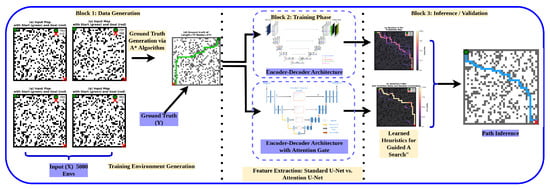
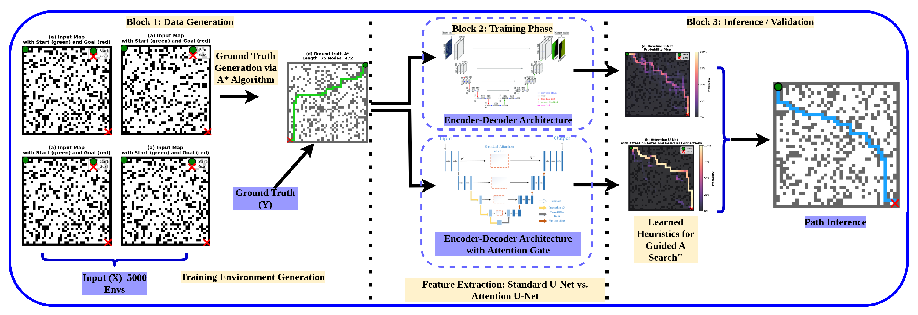
Figure 1 illustrates the overall workflow of our proposed attention-guided path planning framework. Specifically, it depicts the end-to-end pipeline we designed to transform the computational heavy lifting required by classical search into fast learned inference.
Figure 1.
Overview of the proposed attention-guided path planning framework. The workflow illustrates the transformation of classical search into fast learned inference. The left side shows the generation of the synthetic dataset using A*, the middle section depicts the training of the neural network architectures, and the right side demonstrates the final hybrid planning. In the map visualizations, green elements denote start positions, red elements denote goal positions, and blue lines indicate the planned paths.
First, the system generates a synthetic dataset of random occupancy grid maps where the optimal path is computed using A*, acting as an expert demonstrator. This ground truth data is then used to train two deep neural network architectures: a standard U-Net and our proposed Attention U-Net. The models learn to predict a probability map that highlights the optimal traversal area. Finally, these predicted maps serve as learned heuristics to guide the A* search, significantly pruning the exploration space while ensuring optimal pathfinding.
A* is used as the benchmark and expert label generator for three reasons: (i) with an admissible heuristic on grid maps, it provides deterministic shortest-path labels suitable for stable supervision, (ii) compared to Dijkstra, it preserves optimality while reducing unnecessary expansions via heuristic guidance, and (iii) unlike sampling-based planners such as RRT*, it avoids stochastic label variability that can weaken the consistency of pixel-level trajectory supervision.
1.1. Contributions
Our main contributions are:
- Novel Architecture: We propose an Attention U-Net architecture specifically designed for path planning. This architecture combines:
- Attention gates in skip connections for feature selection, enabling the model to focus on path-relevant regions.
- Residual connections in convolutional blocks for improved gradient flow.
- U-Net encoder–decoder structure with skip connections for dense prediction.
- Superior Performance: We demonstrate that Attention U-Net + A* achieves superior performance compared to classical A*: it expands 62% fewer nodes (207.6 vs. 543.11) while maintaining near-optimal path lengths (99.8% of optimal) and faster planning time (0.78 ms vs. 1.19 ms).
- Hybrid Planning Approach: Instead of claiming novelty for learning-guided planning in general, we contribute a task-specific integration for 2D occupancy grids: Attention U-Net probability maps are embedded into weighted A* cost shaping. This hybrid design provides a practical efficiency–optimality trade-off with consistently high success rates and near-optimal paths.
1.2. Paper Organization
The rest of this paper is organized as follows: Section 2 presents related work on path planning and deep learning for robotics. Section 3 describes our approach to path planning using deep learning for robotics. Section 4 describes the experimental setting and outcomes. Section 5 discusses the implications of this work. Section 6 presents concluding remarks on this work and suggestions for further research.
2. Related Work
In this section, we provide a detailed literature review of path planning techniques, both classical and machine learning-based. We discuss the pros and cons of both types of techniques and identify the research gap filled by our study.
2.1. Classical Path Planning
In this context, Kabir et al. [10] have proposed a significant improvement in the A* search strategy by introducing a Robot Motion Block, accompanied by an adaptive cost function, which reduces the number of explored nodes by nearly 94%, thus significantly increasing the rate of convergence compared to traditional A*. At the same time, in order to effectively handle the kinematic constraints associated with robotic motion, a bidirectional A* search strategy has been proposed by Yin et al. [11], which incorporates the scale factor as well as the angle factor in the cost function. Furthermore, in order to eliminate the angular properties associated with the motion planning in a grid-based environment, a cubic B-spline curve smoothing strategy has been integrated with the proposed bidirectional A*. The importance of such a strategy has been highlighted in a previous study by Duchon et al. [12], which discussed the importance of “any-angle” search algorithms, such as Theta* or Phi*, in order to effectively handle the geometric limitations associated with a traditional grid-based motion planning strategy. Considering the limitations associated with the use of deterministic motion planning algorithms in high-dimensional spaces, RRT* has gained significant popularity as a motion planning strategy, as discussed in the literature. However, the limitations associated with the slow rate of convergence have forced researchers to propose directional biases in motion planning algorithms.
Fan et al. [13] suggested the hybrid approach combining rapidly exploring random trees (RRT*) with the artificial potential field (APF) approach for the path planning problem of the UAV. Through the application of the goal-biased approach, the blindness caused by the random approach can be well resolved. With a similar aim of improving environmental adaptability, the DBVSB-P-RRT* algorithm was proposed by Guo et al. [14] and was shown to reduce planning time by more than 40%.
Other researchers have focused on the intrinsic quality of the search tree. Dong et al. [15] proposed the FHQ-RRT* algorithm, which is motivated by dynamic sparse sampling and the generation of “KeyPoints” to optimize the selection of the parents, while Zhu et al. [16] proposed the dual-weighted RRT* algorithm (GAO-RRT*), which directs the search tree towards the goal as well as the proximate obstacles to reduce the path length, contrary to the traditional belief in the advantage of the broader obstacle avoidance.
More recently, the trend with the greatest promise is related to the combination of traditional planners and techniques from artificial intelligence and deep learning. The latter techniques frequently try to address local minimum problems, common in reactive approaches. For example, Zhang et al. [17] proposed a system that integrates A*, the dynamic window approach (DWA), and deep Q-networks (DQNs). In the proposed system, the agent is responsible for making decisions on how the robot can change trajectories in real-time. In other words, the agent is responsible for escaping dead ends, where reactive techniques may fail. In another example, Song et al. [18] proposed an approach related to the integration of obstacle prediction techniques. The authors proposed an approach that integrates a Random Forest classifier, an S-RRT algorithm, and Ant Colony Optimization. The proposed approach demonstrates how supervised learning can be employed to significantly enhance local obstacle avoidance techniques. For 3D environments, another approach related to the combination of enhanced potential fields and B-spline curves has been proposed by Liu et al. [19]. Recent studies also highlight complementary planning directions that are closely related to the present motivation. Menon et al. propose a homotopy-aware, efficiently adaptive state-lattice strategy for cluttered mobile-robot navigation, where the key idea is to preserve topological diversity of feasible route classes while keeping search tractable [20]. Li et al. introduce an obstacle-avoiding manipulator planner based on recursive segmentation point migration combined with progressive inverse kinematics, aiming to improve collision-safe convergence in constrained workspaces [21]. Zhang et al. present a cosine-similarity-based multi-target planning method for cable-driven manipulators, focusing on efficient target ordering and reduced overall traversal cost in multi-goal tasks [22]. Hu et al. develop an efficient RRT-based kinodynamic framework for wheeled robots that jointly targets motion feasibility, smoothness, and path compactness under dynamic constraints [23]. Collectively, these studies reinforce the value of integrating structural priors, optimization mechanisms, and computational efficiency in modern robotic planning systems.
2.2. Machine Learning-Based Approaches
While classical and sampling-based algorithms rely on explicit geometric calculations, the recent paradigm shift toward machine learning (ML) enables robots to learn navigation policies directly from environmental data or expert demonstrations. This change can be best illustrated with regard to the domain of Deep Reinforcement Learning (DRL), wherein agents are able to achieve the best strategies via trial-and-error-based learning. This can be best explained with regard to the initial work done by Lei et al. [24] on the application of the Double Deep Q-Network (DDQN) with regard to the development of dynamic path planning in environments that are not well known. This approach was able to mitigate the instability that often comes with the application of the traditional Q-learning approach, resulting in the development of the path planning approach without the need for any initial maps. Building on the initial work done on the application of the DDQN approach, Zhang et al. [25] were able to address the problems that often come with the application of the initial approach with regard to the development of the path planning approach via the application of the GAP-SAC approach. This approach was able to allow the robots to better attend to the environmental features with the application of the gated attention mechanism, resulting in better performance compared to the application of traditional algorithms like the TD3. Moreover, the work done by Jaramillo-Martínez et al. [26] emphasized the need for the application of the reward shaping approach with regard to the application of the reinforcement learning approach. This was done via the development of the reward function strategy that can help in minimizing not only the distance but also the turns, resulting in the achievement of a 50% reduction in turns with regard to the application of the classical A* approach. Parallel to RL, Supervised Learning and Imitation Learning have been utilized to mimic expert behaviors while reducing computational overhead. Chehelgami et al. [27] introduced a safe global path planning method based on Recurrent Neural Networks (RNNs). They designed a novel loss function that not only learns the path generation but also enforces an adjustable safety margin around obstacles, allowing for the rapid generation of collision-free paths in constant time. Similarly, Waga et al. [28] explored learning from demonstration (LfD) to transfer the optimality of the A* algorithm to a machine learning model. By employing ensemble methods to learn from an “expert” A* planner, they enabled mobile robots to acquire robust navigation policies that mimic optimal behaviors without the heavy runtime search cost associated with classical planners. Most recently, research has expanded into advanced perception and large language models (LLMs) to handle high-level reasoning and complex unstructured environments. In agricultural robotics, Diao et al. [29] proposed a navigation line extraction algorithm based on an improved YOLOv8s network. By combining deep learning-based visual detection with the least squares method, they achieved high adaptability in extracting navigation paths for corn-spraying robots in complex field environments. Pushing the boundaries of cognitive navigation, Waga et al. [30] introduced a hierarchical framework leveraging GPT-4o mini. Their approach utilizes the LLM as a high-level planner to set general waypoints based on contextual reasoning, while an ensemble learning model handles low-level action execution. This hybrid structure combines the semantic understanding of large language models with the precise control of traditional learning methods, marking a significant step toward intelligent, reasoning-capable autonomous navigation.
2.3. Research Gap
Although path planning has been extensively studied, there remain critical gaps that prevent it from being applied well in reality. Based on a review of classical path planning algorithms [10,11,12,13,14,15,16,17,18,19] and learning-based path planners [24,25,26,27,28,29,30], there are three major gaps: (1) classical path planners have computational costs that limit their application to real-time situations, (2) current learning-based path planners do not incorporate attention mechanisms specific to path planning tasks, and (3) hybrid approaches have not been able to achieve both efficiency and near-optimality. Our proposed Attention U-Net model remedies all three gaps by incorporating attention gates, probability maps learned to guide A* searches optimally, and a 62% reduction in node expansions with near-optimal paths. Table 1 summarizes the gaps and our contributions.
Table 1.
Summary of identified research gaps and contributions.
3. Proposed Methodology
In this section, we outline our approach to the learning process in path planning. This begins with a formal definition of the path planning problem and the formulation of the mathematical framework. Next, we introduce the baseline architecture, followed by the proposed architecture incorporating the attention mechanism. Finally, we define the loss functions used for the path planning tasks and the training process used to train the model to learn the heuristics.
3.1. Problem Formulation
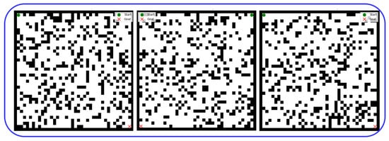
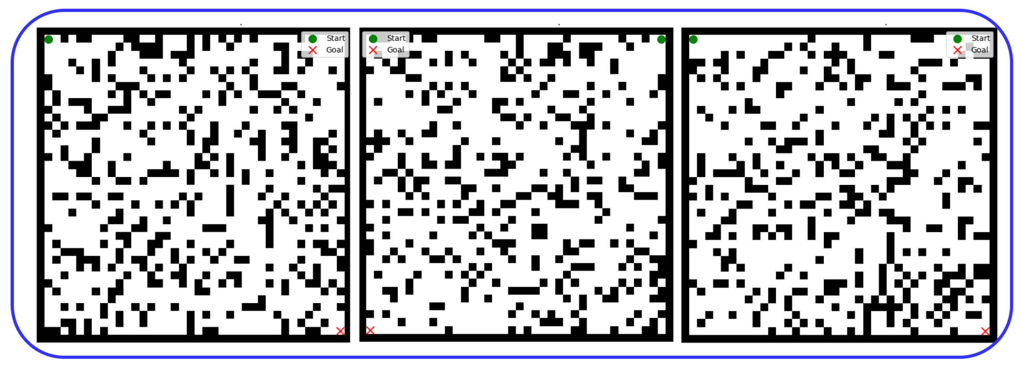
We consider the problem of predicting robot trajectories in 2D grid environments (Figure 2). The input consists of the following:
Figure 2.
Illustrations of binary occupancy grid maps representing 2D environments with robot start and goal locations.
- Occupancy Grid Map : Binary grid where 1 represents free space, and 0 represents obstacles or boundaries. In our experiments, .
- Start Position : Initial robot position, where and (start must be in free space).
- Goal Position : Target position, with the same constraints as the start position.
The output is a trajectory mask where indicates that the cell is part of the predicted path. Ideally, the predicted path should
- Connect the start s to the goal g (connectivity constraint);
- Avoid obstacles: (feasibility constraint);
- Minimize path length (optimality objective).
We encode the input as a 3-channel tensor :
- Channel 0: Occupancy grid G (normalized to ).
- Channel 1: Start position mask S where if , else 0.
- Channel 2: Goal position mask where if , else 0.
The model learns a mapping that predicts the trajectory mask. The output is a probability map where represents the probability that cell is part of the path. We threshold this probability map to obtain the binary trajectory mask: where is a threshold parameter.
3.2. Baseline Architectures
To provide context for our proposed attention-based U-Net, we start by describing a conventional U-Net model, which serves as the reference model for comparison with our proposal. In addition, a complete understanding of the reference model helps us evaluate the improvements offered by attention mechanisms. In this section, we describe a conventional U-Net model and its modification for solving path planning problems, as detailed in Algorithm 1.
| Algorithm 1 U-Net forward pass for path prediction. |
|
The selection of U-Net as the backbone is motivated by three practical considerations in this study. First, trajectory prediction in occupancy grids is a dense pixel-level task, where preserving fine spatial details (obstacle boundaries, narrow passages, start/goal anchors) is essential; U-Net skip connections are well suited to this requirement. Second, this work targets controlled architectural attribution: by keeping the encoder–decoder family fixed and introducing attention/residual modifications incrementally, the measured gain can be directly attributed to the proposed modules rather than to a wholesale backbone change. Third, under the current CPU-oriented experimental setting and training budget, U-Net provides a stable and computationally tractable baseline for fair comparison across variants.
U-Net Baseline
We use a standard U-Net architecture [31] as our deterministic baseline. The U-Net consists of a symmetric encoder–decoder structure with skip connections.
Encoder: The encoder consists of three downsampling blocks. Each block contains:
- Two convolutional layers with a kernel size of 3 × 3 and padding of 1.
- Batch normalization and ReLU activation.
- Max pooling with a stride of 2 for downsampling (except in the last block).
The encoder progressively reduces spatial resolution: , while increasing channel depth: .
Bottleneck: This is a convolutional block that operates at the lowest resolution, which is 5 × 5, with 256 channels.
Decoder: The decoding stage makes use of transposed convolutions (stride of 2) for upsampling, followed by convolutional blocks. Skip connections connect the features of the encoder to those of the decoder at equivalent resolutions.
Output Layer: The channel dimension is reduced to 1 using a convolution, followed by a sigmoid activation to produce probability values ranging from 0 to 1.
The U-Net architecture is especially suited to dense predictions, such as path planning, as the skip connections provide the ability to combine the low-level spatial details (e.g., boundary of obstacles, start/goal points) with the high-level semantic details (e.g., path and connectivity).
3.3. Proposed Attention U-Net
The proposed architecture extends the original U-Net model with attention mechanisms that are carefully designed to improve path planning performance. The key novelty of our approach is the introduction of attention gates in the skip connections, which help the model focus on path information and ignore irrelevant background information. This subsection outlines the architectural design for better performance than the original model, as detailed in Algorithm 2.
We enhance the basic U-Net structure by adding attention gates [32] to the skip connections. The important part is that attention gates enable the decoder to focus on relevant areas of the trajectory using attention coefficients that weight the features of the encoder. An attention gate takes two inputs:
- Gate signal : features from the decoder (upsampled, coarser resolution), where B is the batch size, is the number of gate channels, and is the spatial resolution.
- Skip signal : features from the encoder (finer resolution), where is the number of skip channels and is the spatial resolution.
The attention coefficient is computed through the following steps:
- Feature projection: Both signals are projected to a common intermediate dimension using 1 × 1 convolutions:where and are 1 × 1 convolutional layers with batch normalization.
- Spatial alignment: If and have different spatial dimensions, is upsampled via bilinear interpolation to match :
- Attention coefficient computation: The aligned features are combined and passed through a ReLU activation, followed by a 1 × 1 convolution and sigmoid activation:
The modulated skip connection is then computed via element-wise multiplication:
where ⊙ denotes element-wise multiplication (broadcasting α across the channel dimension). This allows the model to suppress irrelevant background features and focus on path-relevant regions by adaptively weighting encoder features based on decoder context. We also incorporate residual connections within convolutional blocks to improve gradient flow during training. Each convolutional block computes:
This enables training deeper networks and helps preserve important features through the network.
| Algorithm 2 Attention U-Net forward pass. |
|
3.4. Loss Functions
The choice of loss function has a large impact on the quality of predictions of the path. Path planning introduces several unique challenges for loss-function optimization, including class imbalance, because path pixels are a minority, and path continuity. This section describes loss functions to handle these problems, from general loss functions to specially designed loss functions to offer guidance consistent with an A* heuristic.
3.4.1. Standard Losses
We use several loss functions tailored for path planning tasks, each addressing different aspects of the problem. The binary cross-entropy (BCE) [33] loss serves as the standard pixel-wise classification loss, defined as follows:
However, BCE suffers from class imbalance: path pixels are typically less than 5% of the image, causing the model to predict all zeros. To address this limitation, we use Dice loss, which handles class imbalance by focusing on the overlap between predicted and target masks. The Dice loss is defined as follows:
where is the intersection, and are the sums of predicted and target masks, and is a smoothing term. Additionally, we employ a combined loss that integrates multiple objectives through a weighted combination of BCE, Dice, and continuity terms:
where penalizes disconnected paths by measuring the number of connected components, ensuring that predicted paths maintain connectivity from start to goal.
3.4.2. A*-Optimized Loss
In the context of models used as cost heuristics in A*, we introduce a tailored loss function that addresses the unique needs of heuristic search. The basic idea is that A* performance can be enhanced by probability maps that assign high probability to optimal paths with strong peaks and low probability everywhere else to provide a strong contrast, and gradients that transition smoothly to the path rather than making binary predictions. The A*-Optimized Loss combines several components to achieve these goals. To do this, we also include focal loss [34], which focuses on the difficult examples with a high gamma value. The focal loss is given as follows:
where and . The term downweights easy examples (high-confidence correct predictions) and focuses learning on hard examples, which is particularly important for learning precise path boundaries.
To encourage clear probability peaks, we employ sharpness loss, which penalizes flat distributions by measuring the entropy-like term:
This loss is minimized when , encouraging sharp, confident predictions rather than uncertain probability distributions.
Additionally, we use path width loss to penalize overly thick predictions by measuring the average width of predicted paths:
This component encourages the model to predict narrow, precise paths rather than thick regions that may include unnecessary detours.
The total A*-optimized loss integrates all these components through a weighted combination:
with weights , , , and . These weights balance the different objectives, prioritizing focal loss for hard example learning while incorporating Dice loss for overlap maximization, sharpness for clear predictions, and width constraints for path precision, as detailed in Algorithm 3.
| Algorithm 3 A*-optimized loss computation. |
|
3.5. Training Procedure
The training process plays a crucial role in learning useful path planning heuristics. This section outlines the process of dataset generation, training setup, and model evaluation. Each part of the training process is described in depth to guarantee reproducibility. This includes dataset generation, training setup, and model evaluation.
3.5.1. Dataset Generation
In order to train the Attention U-Net model, we create a dataset of 5000 random 40 × 40 grid world environments. This dataset is developed in a systematic manner to ensure the diversity and quality of the training data.
Environment creation follows a multi-step procedure. To begin, an empty grid is created, and obstacles are randomly placed in cells with a given probability in inner cells, while boundary cells are set to obstacles in a deterministic fashion to form confining walls and to ensure that all possible paths stay inside the grid cells. Next, start and end points are chosen from the list of non-obstacle cells; in other words, they are often placed in opposite corners to ensure non-trivial paths requiring navigation around obstacles, but they can be placed anywhere in the free space. The ground truth path is then found using the A* algorithm and Manhattan heuristic, which returns optimal paths useful for training. The obtained path is then represented as a binary mask where path cells have a value of 1, and all other cells have a value of 0.
Each data sample in the dataset is represented as a three-channel tensor, where the channels correspond to the occupancy grid, the start position mask, and the goal position mask. The shape of the input tensor is (3, 40, 40), and the shape of the target is a binary trajectory mask (1, 40, 40). Additional information is stored for every sample, including the start and goal positions, path length, and success flag. The whole dataset is split into a training (80% and 4000 samples) and a validation (20% and 1000 samples) subset, where the validation environments are created with a different random seed to avoid any leakage between the training and validation sets. At this stage, training and test environments are procedurally generated occupancy grids and do not yet include structured floor-plan datasets (e.g., corridor–doorway layouts, office maps, or warehouse maps).
3.5.2. Training Details
Training configuration plays a critical role in achieving good model performance. We use the Adam optimizer [35] with a learning rate of , weight decay of for L2 regularization, and standard beta parameters (, ). The batch size is set to 64 samples per batch, which provides a good balance between training stability and computational efficiency. We tested larger batch sizes (128) but found no significant improvement while requiring more memory.
Training is conducted for a maximum of 50 epochs, with the use of early stopping to prevent overfitting. Training stops automatically if, for 10 successive epochs, the validation loss does not improve (patience = 10), and the model with the lowest validation loss is saved. To better train the model, a ReduceLROnPlateau learning rate scheduler is used to decrease the learning rate by a factor of 0.5 if the validation loss has plateaued for 5 successive epochs.
In order to improve generalization and robustness, data augmentation is performed during the training procedure. This involves randomly flipping the images horizontally and vertically with a probability of 0.5 for both, and randomly rotating them by 90 degrees (choices are 0, 90, 180, and 270 degrees) with the same probability. The start and destination points are transformed based on the data augmentation.
All training is performed on a CPU. The training process is computationally intensive, with typical training time for 50 epochs taking approximately 11 h on a standard CPU. To prevent overfitting and improve generalization, we apply several regularization techniques. Dropout with probability is applied in convolutional blocks, batch normalization is used after each convolution to stabilize training, and weight decay provides L2 regularization where .
3.5.3. Evaluation Metrics
To properly analyze the effectiveness of our Attention U-Net model, we use a variety of evaluation metrics that measure different aspects of path planning. Using these evaluation metrics, we can analyze not only the direct prediction task but also the effectiveness of our model as a heuristic for traditional planning algorithms, as detailed in Algorithm 4.
Success Rate: Percentage of environments where the predicted path connects the start to the goal. A path is considered successful if there exists a connected sequence of cells from start to goal in the predicted mask. We check connectivity using breadth-first search.
Path Length: Average length of successful paths, measured as the number of cells in the path. We compare against the optimal A* path length.
IoU (Intersection over Union): Overlap between predicted and ground-truth masks:
where P and T are predicted and target binary masks (after thresholding).
Node Expansions: For hybrid approaches (learned model + A*), the number of nodes explored by A* during planning. This measures the efficiency of the learned heuristic.
Inference Time: Wall-clock time to compute a prediction, measured in milliseconds. This includes the model forward pass and any post-processing.
| Algorithm 4 Model training pipeline. |
|
4. Experiments and Results
This section presents a thorough analysis of the Attention U-Net technique for path planning. The technique is compared with classical planning algorithms with regard to its performance across a set of parameters. The subsequent subsections cover the experimental environment, direct prediction results, hybrid planning results, and analysis.
4.1. Experimental Setup
We compare all models on a held-out test set of 200 procedurally generated environments. The procedurally generated environments are created in the same way as in the training data, but with a different random number seed. For each model, we measure:
- Direct trajectory prediction performance: How well the model predicts paths directly, without integration with classical planners.
- Performance as cost heuristic: How well the model guides A* planning when used as a cost function.
We compare against classical planners:
- A*: Optimal path with Manhattan heuristic .
- Dijkstra: Optimal path without heuristic (equivalent to A* where ).
- Greedy: Greedy best-first search using only the heuristic (no cost accumulation).
All experiments are conducted on a machine with an Intel i7-9700K CPU. All training and inference operations are performed on the CPU. This CPU-only setup reflects real-world deployment scenarios where a GPU may not be available, making our results directly applicable to resource-constrained environments.
4.2. Direct Trajectory Prediction
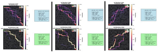
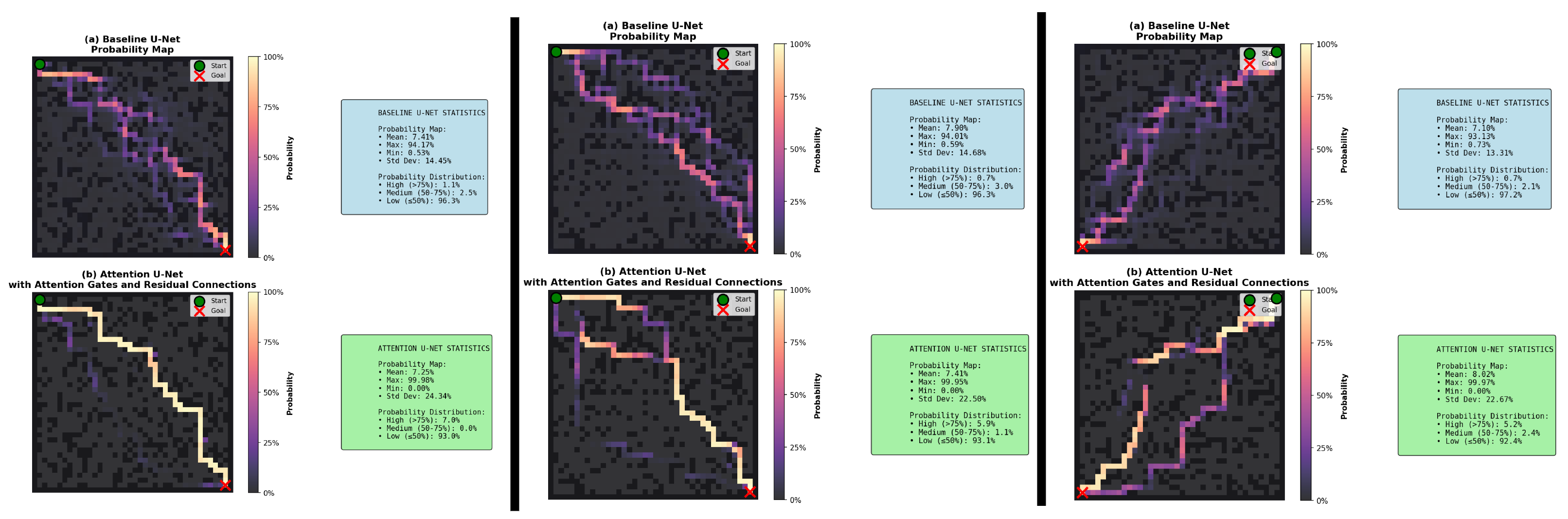
Before integrating our learned model with classical planners, we first evaluate its direct trajectory prediction capability. This analysis helps us understand how well the model can predict paths independently, without assistance from search algorithms, as shown in Figure 3.
Figure 3.
Direct trajectory prediction comparison across three sample environments. For each environment column: (a) the top row shows the probability map generated by the Baseline U-Net; (b) the bottom row displays the highly focused probability map generated by the proposed Attention U-Net. The heatmaps illustrate the predicted probability of a cell belonging to the optimal path, as indicated by the color bars (0% to 100%). Green circles denote start positions, and red stars indicate goals. The accompanying boxes detail the statistical distribution of the predicted probabilities for each respective model.
4.3. Obstacle-Density Shift Robustness
To address robustness under distribution shift, we conducted an additional density-shift experiment using the same 40 × 40 protocol while varying obstacle probability at test time (). For each density, we evaluated 100 solvable environments and compared A*, Baseline U-Net + A*, Attention U-Net + A*, and GNN + A*. As detailed in Table 2.
Table 2.
Density-Shift Evaluation Across Obstacle Probabilities (100 solvable maps per density).
The results indicate that the proposed Attention U-Net guidance remains effective across sparse, nominal, and cluttered settings. Relative to classical A*, node expansions are reduced by 50.4% at p = 0.10, 61.7% at p = 0.25, and 10.5% at p = 0.40. This confirms that the efficiency gain is not restricted to a single obstacle density, while also showing that gains decrease in highly cluttered maps where detours are structurally constrained.
4.4. Ablation Study
To understand the importance of individual architectural elements, we perform an ablation study on attention mechanisms and residual connections. Through this, we are able to determine which elements are of the utmost importance to ensure that there is optimal performance. An ablation study is done to determine the importance of individual elements of the Attention U-Net. Table 3 shows the results when used as A* heuristics.
Table 3.
Ablation study: component contributions (node expansions).
The ablation study focuses on the critical importance of the role of attention mechanisms in achieving better performance. Adding the attention gates to the baseline U-Net significantly decreases the number of node expansions, reducing it by 57% from 480.2 to 207.6. This significant decrease in the number of expansions confirms the effectiveness of the proposed model in utilizing the guidance provided by the A* search by allowing it to focus on the relevant areas, thanks to the feature modulation by the attention gates.
The residual connections, while not directly impacting the reduction of node expansions in this setup, play an important role in the overall quality of the model. The model’s training can benefit from improved gradient flow, which indirectly supports the efficiency of attention mechanisms. The synergy created from the use of attention gates and residual connections creates an efficient framework in which attention is applied to well-learned features.
To strengthen state-of-the-art contextualization, we additionally report a GNN + A* baseline in this section. In our benchmark, GNN + A* expands substantially more nodes than both Baseline U-Net + A* and Attention U-Net + A*. This behavior suggests that, in the current grid setting and training configuration, the tested GNN prior does not provide a sufficiently informative cost surface for A* pruning. In contrast, the attention-gated U-Net produces sharper path-relevant probability maps, yielding stronger search-space reduction.
The key result here is that attention mechanisms are the key reason for the observed boost in performance, allowing Attention U-Net to outperform the classical A* algorithm by a significant 62% in terms of node expansions. This becomes possible as the network focuses its computations on areas that are relevant to the path, unlike the uniformity of spatial locations in the previous approach.
4.5. Sensitivity Analysis of the Cost Weight λ
To justify the selection of λ = 10, we evaluated and measured success rate, average path length, node expansions, and runtime. As detailed in Table 4.
Table 4.
Sensitivity analysis for cost weight λ in learned-guided A*.
The results indicate that λ = 10 offers the best compromise in our setting, with strong search reduction while preserving near-optimal path quality and 100% success.
4.6. Search Space Visualization: Search Cones
To visually demonstrate the efficiency gains of our approach, we visualize the search cones—the set of nodes explored during path planning—for both classical A* and Attention U-Net + A*. These heatmaps provide intuitive evidence of how learned heuristics dramatically reduce the exploration space while maintaining path optimality.
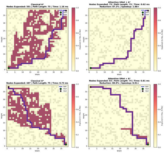
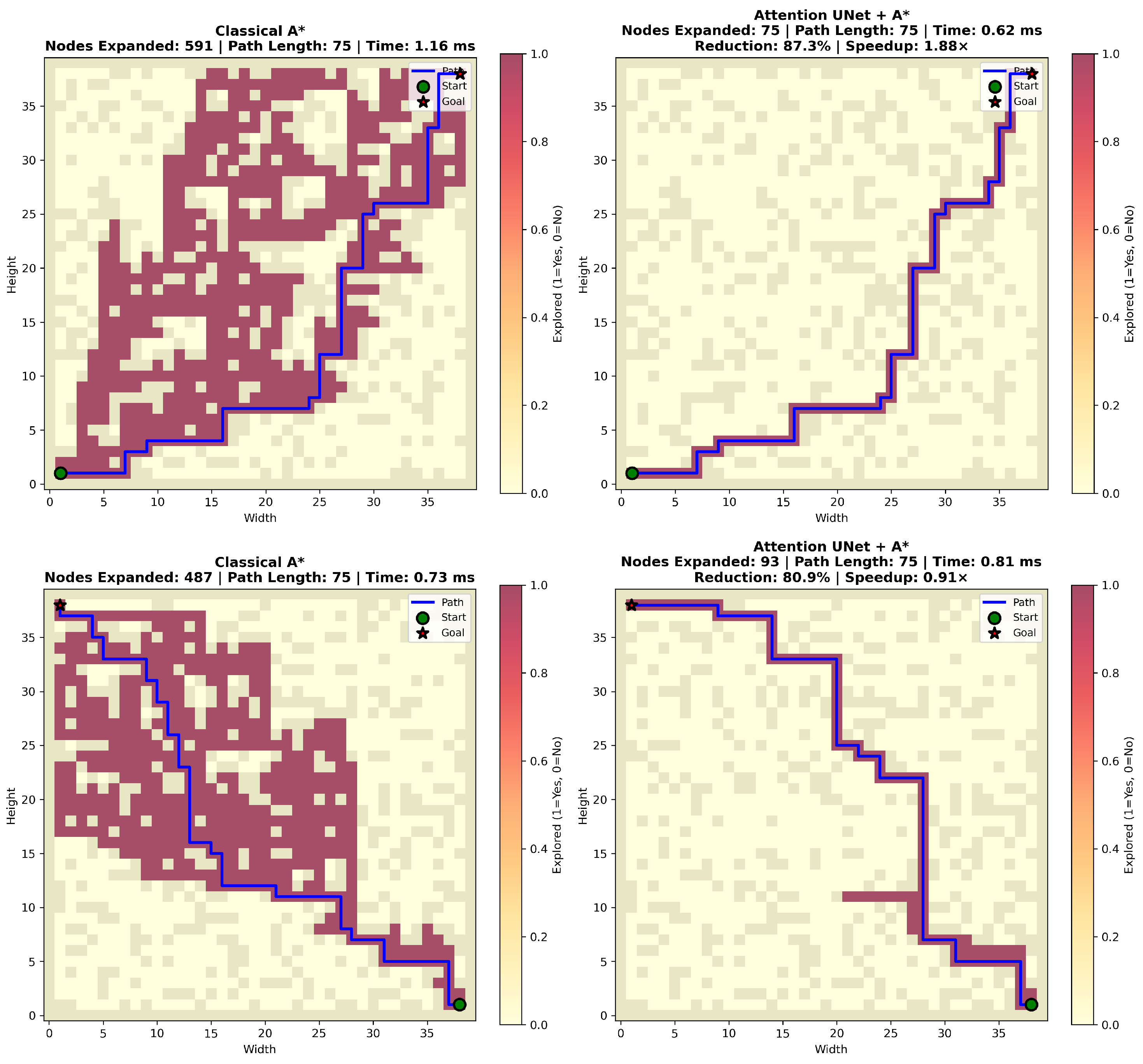
Figure 4 presents side-by-side comparisons of search cones for two representative environments. The heatmaps show explored nodes (red/yellow regions) overlaid on the environment grid, with the optimal path highlighted in blue. Start and goal positions are marked with green circles and red stars, respectively.
Figure 4.
Search cone comparison for two representative environments (top row and bottom row). The left column displays the unconcentrated search space of Classical A* (e.g., exploring 591 nodes), whereas the right column shows the highly focused search space of Attention U-Net + A* (e.g., exploring only 75 nodes, an 87.3% reduction). The heatmap colors (red/yellow) visualize the explored nodes overlaid on the grid. Start positions are marked with green circles, goals with red stars, and optimal paths are highlighted in blue. The intentional overlapping of the heatmap over the grid visualizes exploration density and does not affect scientific understanding.
The classical A* cone (left panel) shows an unconcentrated exploratory pattern, with large areas of the environment explored. In comparison, the Attention U-Net + A* algorithm produces a highly concentrated search cone around the optimal path, with the algorithm exploring only 75 out of 591 possible nodes, representing an 87.3% reduction.
Such visualizations of the explored search cones give us compelling reasons to believe that the superior efficiency of the proposed Attention U-Net + A* method comes from the ability of the method to focus the exploration on the more relevant parts of the paths, thus confirming the findings of the numerical experiments. This significant reduction in the number of explored nodes while maintaining the optimality of the paths clearly proves the efficiency of the learned heuristics.
4.7. Computational Efficiency
Computational efficiency is crucial for real-time robot navigation. We analyze the time complexity and practical performance of our approach compared to classical methods, considering both inference overhead and planning time.
Table 5 compares inference times for different methods.
Table 5.
Computational efficiency comparison.
Attention U-Net + A* achieves faster total planning time (0.78 ms vs. 1.19 ms for A*), despite adding 0.15 ms inference overhead. This is because the reduction in node expansions (62% fewer) more than compensates for the inference cost. Both methods are fast enough for real-time applications (sub-2 ms). Attention U-Net + A* is 34% faster than classical A*, making it particularly suitable for high-frequency control loops.
4.8. Hybrid Planning: Learned Models as Cost Heuristics
The key significance of this research lies in using learning models to guide traditional planning algorithms. This approach combines the efficiency of learned heuristics with the optimality properties of the A* search algorithm. In the next section, we explain the methodology and results related to this approach.
We are aware of the integration of the learned models with A* through the use of predicted probability maps in the cost function. This is achieved through the modification of the cost function in A*:
where is the predicted probability at node n, and λ is a weighting factor (we use λ = 10). This encourages A* to prefer nodes with high predicted probability while still maintaining optimality guarantees (since we add a bounded term to the heuristic), as detailed in Algorithm 5.
The quantitative performance metrics for all evaluated planning methods are detailed in Table 6.
| Algorithm 5 Hybrid planning: learned model + A* |
|
Table 6.
Hybrid planning results: classical and learning-based baselines.
Attention U-Net + A* achieves superior performance compared to classical A* [5,10]: it expands 62% fewer nodes (207.6 vs. 543.11) while maintaining near-optimal path lengths (99.8% of optimal, 75.80 vs. 75.42) and faster planning time (0.78 ms vs. 1.19 ms). The added Baseline U-Net + A* row confirms that the gain is specifically associated with attention-enhanced feature gating, not only with generic learning-based guidance. To address state-of-the-art comparison concerns, we additionally report a GNN + A* baseline in the same table under the same benchmark protocol. All methods achieve 100% success rate, demonstrating robustness. This is expected for A*-based methods, which guarantee finding a path if one exists. The learned heuristics successfully guide A* without causing failures, validating that learned models can be safely integrated with classical planners.
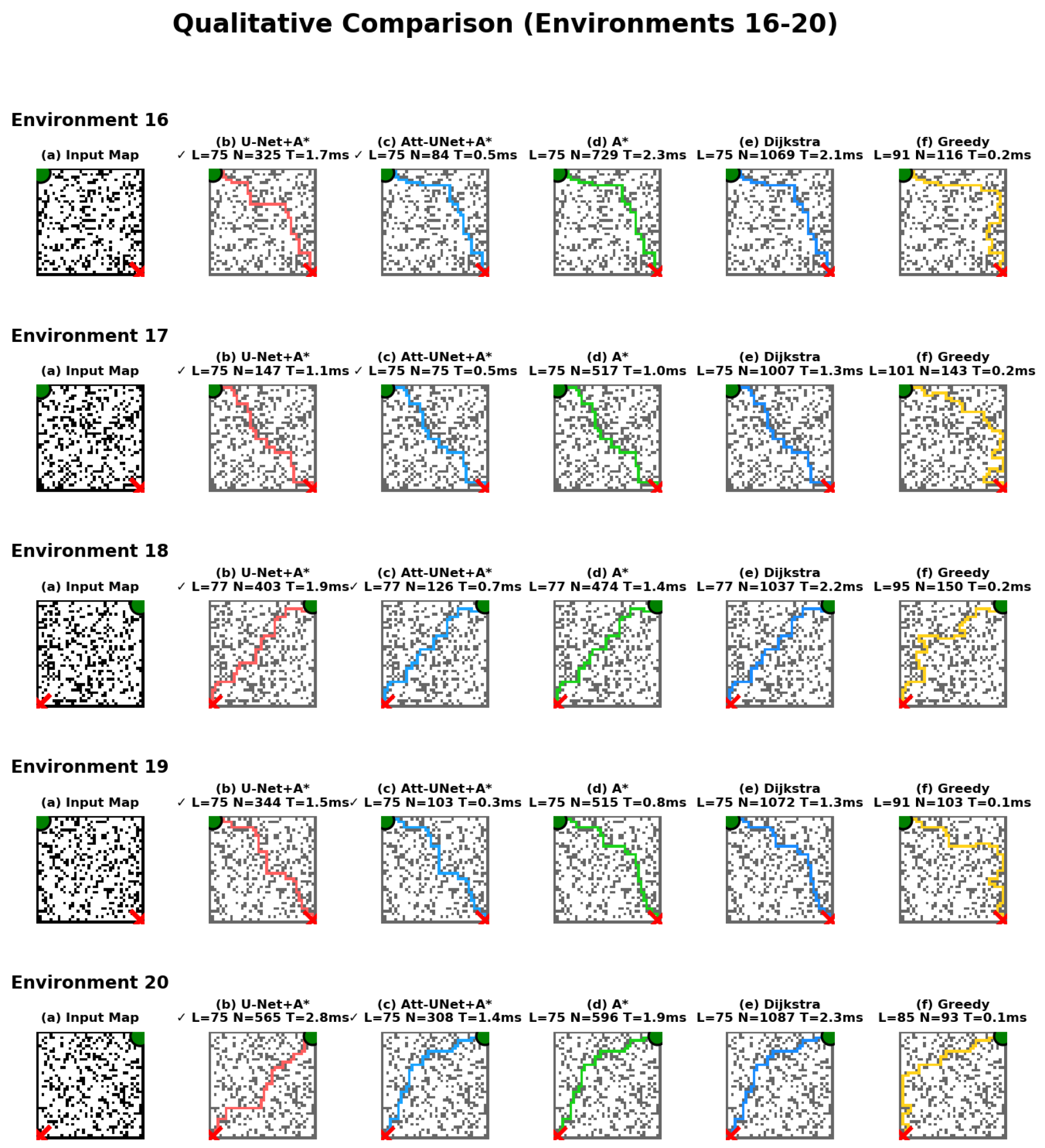
This demonstrates that properly designed learned heuristics with attention mechanisms can outperform classical methods. Attention U-Net + A* achieves superior overall performance: 62% fewer node expansions AND faster planning time. This is because fewer node expansions more than compensate for the model inference overhead. The attention mechanisms enable the model to focus on path-relevant regions, leading to more effective guidance for A*. Attention U-Net + A* maintains near-optimal path lengths (99.8% of optimal), demonstrating that the reduction in node expansions does not come at the cost of path quality. The learned heuristic successfully guides A* toward optimal paths more efficiently than the Manhattan heuristic. The attention mechanisms in skip connections enable the model to focus on path-relevant regions while suppressing irrelevant background features. This selective attention leads to more effective guidance for A*, resulting in fewer node expansions. Further qualitative results, including visualizations of the predicted paths and search spaces across 20 different test environments, are provided in Appendix A.
5. Discussion
This section analyzes our experimental results. We examine classical and learned path planning approaches. We discuss when each approach is most appropriate. We also explore how hybrid integration creates synergistic benefits.
5.1. Performance Analysis and Comparative Advantages
Compared to traditional A*, Attention U-Net performs better. Attention U-Net keeps nearly optimal paths at the cost of exploring 62% fewer nodes. Nonetheless, this is merely one aspect of their comparison. A discussion on the basic differences between these two is justified.
In classical planners, such as A* and Dijkstra, optimality is assured by the use of admissible heuristics. They offer search algorithms that are easy to understand and require no learning. This makes them the best choices in scenarios where optimality is a necessity and ease of interpretation is a priority, for instance, in safety-critical tasks. They are suitable in scenarios where the environment is faced only once. However, in classical planners, the search space has to be searched explicitly, leading to computational complexities proportional to the complexity of the environment. The average number of nodes expanded for the classical A* algorithm in our simulation is 543.11.
In addition to classical heuristics, learned models can find patterns that are indicative of the necessity for specific path configurations. These patterns may not always be visible to human designers, and their use becomes more beneficial as environmental complexity increases. The complex correlations between paths and configurations are hard to represent by human-designed heuristics. Moreover, learned models allow for customization, which helps to adapt to a particular scenario, robot constraints, or tasks by adjusting the loss function or training data, without requiring a change in the planner algorithm.
A* search is still a necessary part of hybrid approaches. Nevertheless, machine-learned models can also provide direct and search-free predictions of paths. This is useful in environments with limited computational capabilities. The development of direct predictions marks a paradigm shift in which prediction-driven planning eclipses search-driven planning. In environments in which search costs are too high, there are new opportunities. As machine learning models continue to evolve and larger training sets become available, machine-learned heuristics promise to be superior to classical heuristics in more challenging environments in which hand-coded heuristics fail. This study establishes a foundation for this future direction.
5.2. Method Selection Criteria and Practical Guidelines
The choice between the learned planner and the classical planner depends on a set of conditions such as performance requirements, availability of data, computational power, and nature of the problem. It helps in recognizing the appropriate approach in methodological considerations.
The synergy of Attention U-Net and A* is beneficial when performance is of utmost importance. This method performs well when dealing with scenarios involving frequent interactions of similar types of environments. Empirical studies show that there is a node expansion reduction of 38–62% compared to traditional A* (207.6–360.9 nodes vs. 543.11 nodes), as well as reduced planning times of 0.78 ms vs. 1.19 ms. In cases involving frequent interaction with the same environment type, the training overhead is justified by the fact that the cost of training is spread across several planning queries. In complex cost environments, the hybrid approach is more beneficial as environments with non-uniform costs are better approximated by learned models compared to traditional heuristics. Transfer learning environments also benefit from the ability of the learned model to generalize, which is more beneficial when dealing with environments that are unfamiliar and have few data samples. In complex path planning problems, which are difficult to approximate using traditional heuristics, learned models can easily incorporate these using training data or loss functions.
Classical A* is still the best choice in situations where training data are not available. It is most appropriate in one-shot planning tasks, especially in situations where the same environment is not likely to be visited more than once, in which case training overheads would not make sense. Classical planning offers solutions immediately, without having to build any model. In addition, concerns over interpretability might make classical planning more attractive, especially in situations such as self-driving cars, in which the reasoning behind the selected route would need to make sense. In classical planning, the search processes are transparent and can thus be checked. In situations where computational infrastructure to infer models is not available, classical A* offers a direct solution. It can also act as a simple baseline, not having any overheads related to model loading or inference.
The hybrid approach represents an optimal compromise. It provides superior performance while maintaining optimality guarantees. The approach achieves 38–62% fewer node expansions than classical A*. It maintains near-optimal paths (99.4–99.8% of optimal). It achieves 100% success rate with learned guidance. Faster planning times (0.78–0.97 ms vs. 1.19 ms for A*) make it suitable for high-frequency control loops. Computational efficiency is critical in such applications.
To better contextualize modern learning baselines, we implemented and integrated a GNN-guided planning comparison under the same environment generation protocol as the U-Net family and classical planners. This additional baseline strengthens the architectural comparison and confirms that the proposed attention-based design remains the most efficient in node expansion reduction. DRL-based comparisons are identified as a dedicated next step and are discussed as future work to avoid over-claiming beyond the currently reported benchmark table.
5.3. Hybrid Planning Architecture: Synergistic Integration
Moreover, the benefits of the learned models and those of the classical A* search algorithms complement each other in a way that is synergistic and exceeds the benefits of each approach individually. The proposed approach of fusing two techniques is expected to take the advantages of each approach, where the efficiency and pattern recognition of the learned models can be leveraged.
The performance advantages are dramatic. Attention U-Net, together with A*, cuts the number of nodes visited by 62% compared to classical A* (207.6 vs. 543.11 nodes), and correspondingly cuts planning times (0.78 ms vs. 1.19 ms). The improved performance is due to the learned model’s ability to focus the A* search on regions of the path that are relevant to the search, thus avoiding unnecessary regions of the configuration space. Notably, all improved models maintain paths of at most 99.4% to 99.8% of optimal cost, showing that improved performance is not at the cost of path quality. The optimality properties of A* guarantee feasibility and optimality despite errors in the learned model. The learned heuristic informs but does not restrict the search, allowing A* to find near-optimal paths. The method obtains 100% success rate and a competitive path cost. The learned model may not always predict the optimal path, but A* can still find the solution given the probabilities learned.
Beyond performance metrics, the hybrid architecture offers additional benefits. The weighting factor λ in the cost function can be tuned. This balances between learned guidance and classical optimality. It provides flexibility to adapt to different application requirements. For λ = 0, the approach reduces to standard A*. For large λ, it relies more heavily on learned predictions. This tunability allows practitioners to adjust the balance between efficiency and optimality. The learned model can be updated or fine-tuned for new environments. This is done without redesigning the planning algorithm. It enables adaptation to changing conditions or new deployment scenarios. Models can learn complex patterns difficult to encode in classical heuristics. This potentially provides greater advantages in complex environments where classical methods struggle. However, the hybrid paradigm involves certain issues. The models require training data and heavy computational power, which may not be justified in the case of a planning task. The training procedure is time-consuming (11 h on a CPU in the current studies). The performance is dependent on the quality and representativeness of the training data. In the case where test scenarios are significantly different from the training set, the performance may decrease, for example, due to the difference in the number and form of obstacles. Despite the aforementioned issues, the results of the experiment confirm the superiority: the number of nodes is reduced by 62% while maintaining the optimal path length and reducing the planning time.
6. Conclusions, Limitations, and Future Work
This final section provides a comprehensive summary of our work, acknowledges the limitations of our approach, and outlines promising directions for future research. We consolidate our findings, discuss the constraints of our method, and propose extensions that could further advance learning-based path planning.
6.1. Conclusions
This paper introduces a path planning framework for mobile robots that applies attention-based deep learning techniques to improve path planning. The Attention U-Net model introduced applies attention gates to focus on path-relevant areas and assist A* path planning compared to traditional methods.
The results obtained from the experiment show that the Attention U-Net approach using A* has a success rate of 100% on graphs where the legal paths are longer than the optimal path by 0.5%. More importantly, the results show that by incorporating the attention mechanism, there is a reduction of 62% in the number of node expansions compared to the standard A* algorithm, although planning times are still faster by 1.19 ms compared to 0.78 ms.
The implications of these results are such that attention mechanisms play an important role in realizing these performance improvements. By allocating computing resources to areas that are related to the path, rather than allocating an equivalent amount to all spatial regions, A* can result in improved efficiency. The open-source nature of this research will encourage more research in this area.
6.2. Limitations
Despite the proposed method’s superior performance, some limitations need to be taken into account. First, while the proposed method achieves superior performance, it is not optimal. Rather, it achieves near-optimal solutions, which amount to 99.8% optimality, according to the results. This implies that for tasks that require mathematical optimality, classical methods can be used. Second, the proposed method’s ability to generalize may be affected by the nature of the data distribution. This implies that if the test environment varies significantly from the training data, such as in the case of a 100 × 100 grid compared to a 40 × 40 grid, or if the environment contains previously unobserved obstacles, the performance may be affected. Third, compared to classical methods, which have clear logic, the proposed method’s logic, which relies on deep learning, may be difficult to interpret. Finally, with regard to the training time, which requires 11 h for completion, this may be a limitation for some environments that have limited resources. An additional limitation is that the present validation does not yet include structured real-world-like map topologies. Consequently, our current conclusions are restricted to the tested occupancy-grid regime, and broader topology-level generalization remains to be confirmed experimentally.
6.3. Future Work
Future work should be directed toward extending the adaptability range of the system in dynamic environments. It will be essential to integrate temporal modeling architectures, such as long short-term memory networks or Transformer encoders. Additionally, it will be important to test the scalability of the algorithm through experiments conducted on much larger grids (200 × 200 to 500 × 500) in order to determine whether the efficiency improvements are maintained at a larger scale. Additionally, it will be important to extend the robustness tests to a broader range of topologies, including mazes and office floor plans. A prioritized next step is structured-map validation using office/warehouse-style layouts and Moving AI-style benchmarks, under matched protocols and identical metrics (success rate, path length, node expansions, and runtime) to quantify topology-level generalization.
In particular, Transformer-style and self-attention-heavy segmentation backbones are recognized as relevant alternatives and will be evaluated in a dedicated follow-up study under matched training budgets and identical benchmark protocols, to preserve fairness and isolate architectural effects.
Author Contributions
Conceptualization, A.W., S.B. and A.B.; Methodology, A.W., S.B., A.B. and A.R.; Software, A.W. and A.R.; Validation, A.W., S.B., A.B., F.Z.S., J.A. and T.M.; Formal Analysis, A.W. and S.B.; Investigation, A.W., S.B. and A.B.; Resources, A.W., S.B., A.B., F.Z.S., J.A. and T.M.; Data Curation, A.W. and A.R.; Writing—Original Draft Preparation, A.W.; Writing—Review & Editing, S.B., A.B., F.Z.S., J.A., T.M. and A.R.; Visualization, A.W. and A.R.; Supervision, S.B. and A.B.; Project Administration, A.W., S.B. and A.B. All authors have read and agreed to the published version of the manuscript.
Funding
This research received no external funding.
Data Availability Statement
The data and experimental configurations used to support the findings of this study are available from the corresponding author upon reasonable request.
Acknowledgments
The authors gratefully acknowledge the Euromed University of Fez (UEMF), Morocco, for institutional support and the research facilities. During the preparation of this manuscript, the authors used Gemini 3 Flash (Google) for language polishing and sentence reformulation. The authors reviewed and edited the output and take full responsibility for the content of this publication.
Conflicts of Interest
The authors declare no conflicts of interest.
Appendix A. Qualitative Comparison on 20 Test Environments
The following figures illustrate the performance of our Attention U-Net + A* framework compared to other baselines across 20 randomly generated test environments.
Figure A1.
Environments 1–5. For each environment row, the columns represent: (a) Input Map; (b) U-Net + A* (red path); (c) Attention U-Net + A* (blue path); (d) A* (green path); (e) Dijkstra (cyan path); (f) Greedy (yellow path). The green circles denote the start positions and the red stars indicate the goals. The check mark (✓) indicates that the algorithm successfully found an optimal path.
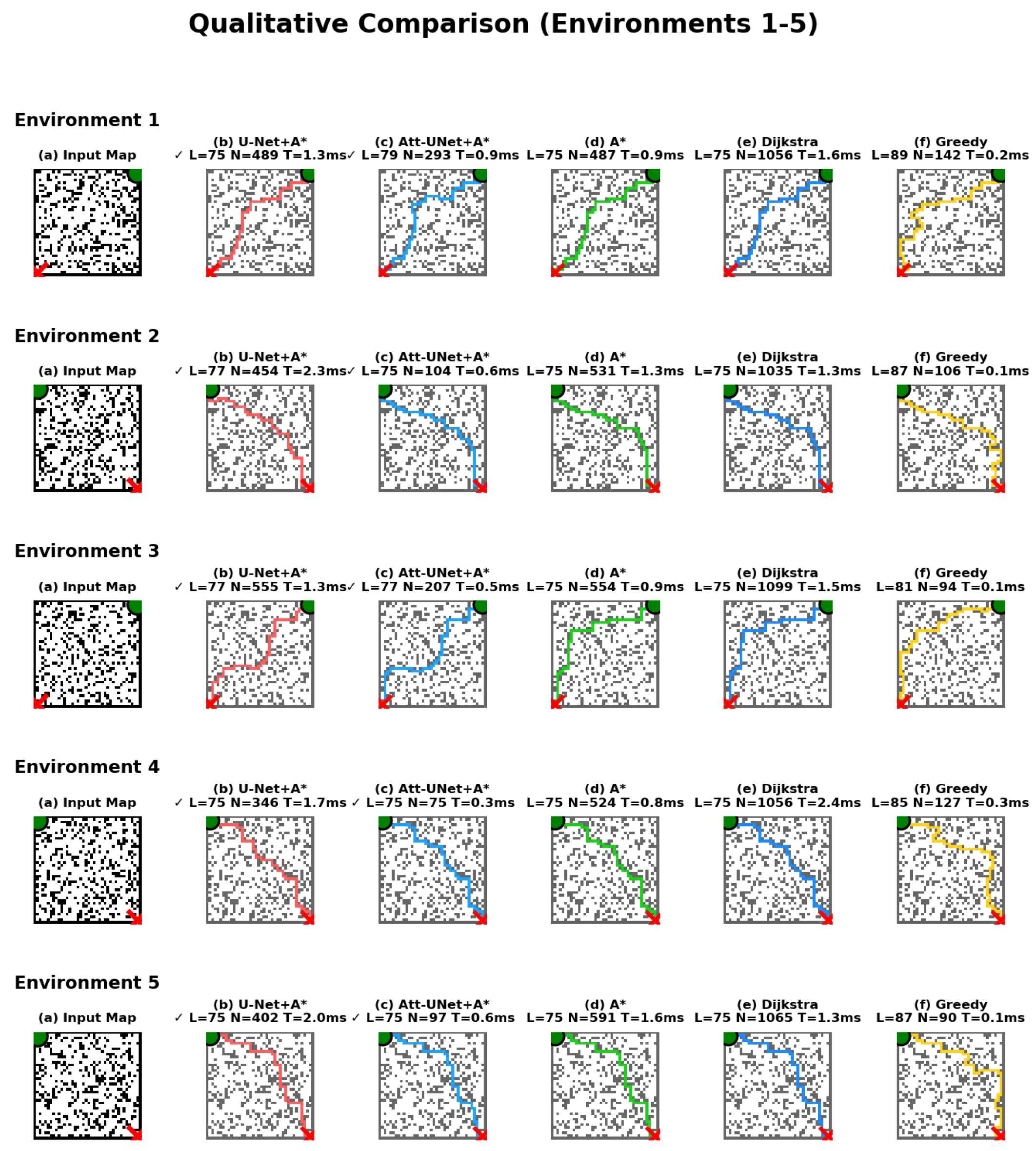
Figure A2.
Environments 6–10. For each environment row, the columns represent: (a) Input Map; (b) U-Net + A* (red path); (c) Attention U-Net + A* (blue path); (d) A* (green path); (e) Dijkstra (cyan path); (f) Greedy (yellow path). The green circles denote the start positions and the red stars indicate the goals. The check mark (✓) indicates that the algorithm successfully found an optimal path.
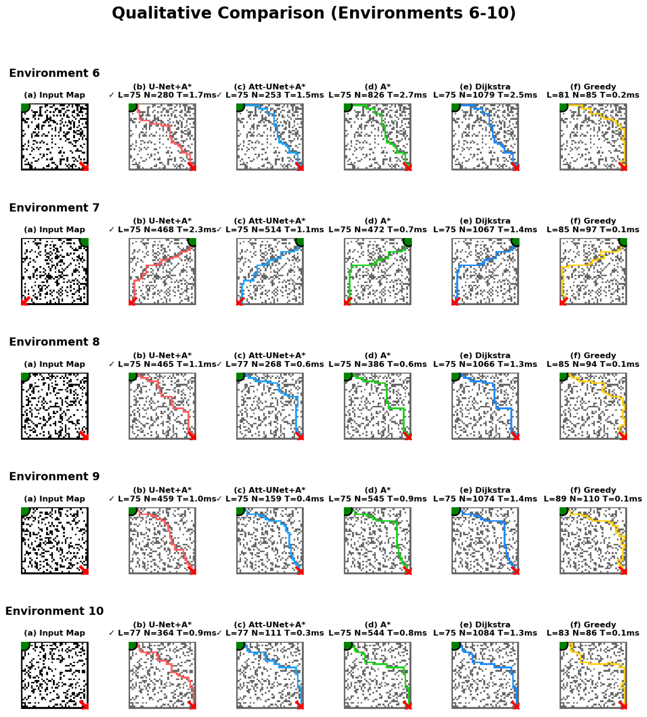
Figure A3.
Environments 11–15. For each environment row, the columns represent: (a) Input Map; (b) U-Net + A* (red path); (c) Attention U-Net + A* (blue path); (d) A* (green path); (e) Dijkstra (cyan path); (f) Greedy (yellow path). The green circles denote the start positions and the red stars indicate the goals. The check mark (✓) indicates that the algorithm successfully found an optimal path.
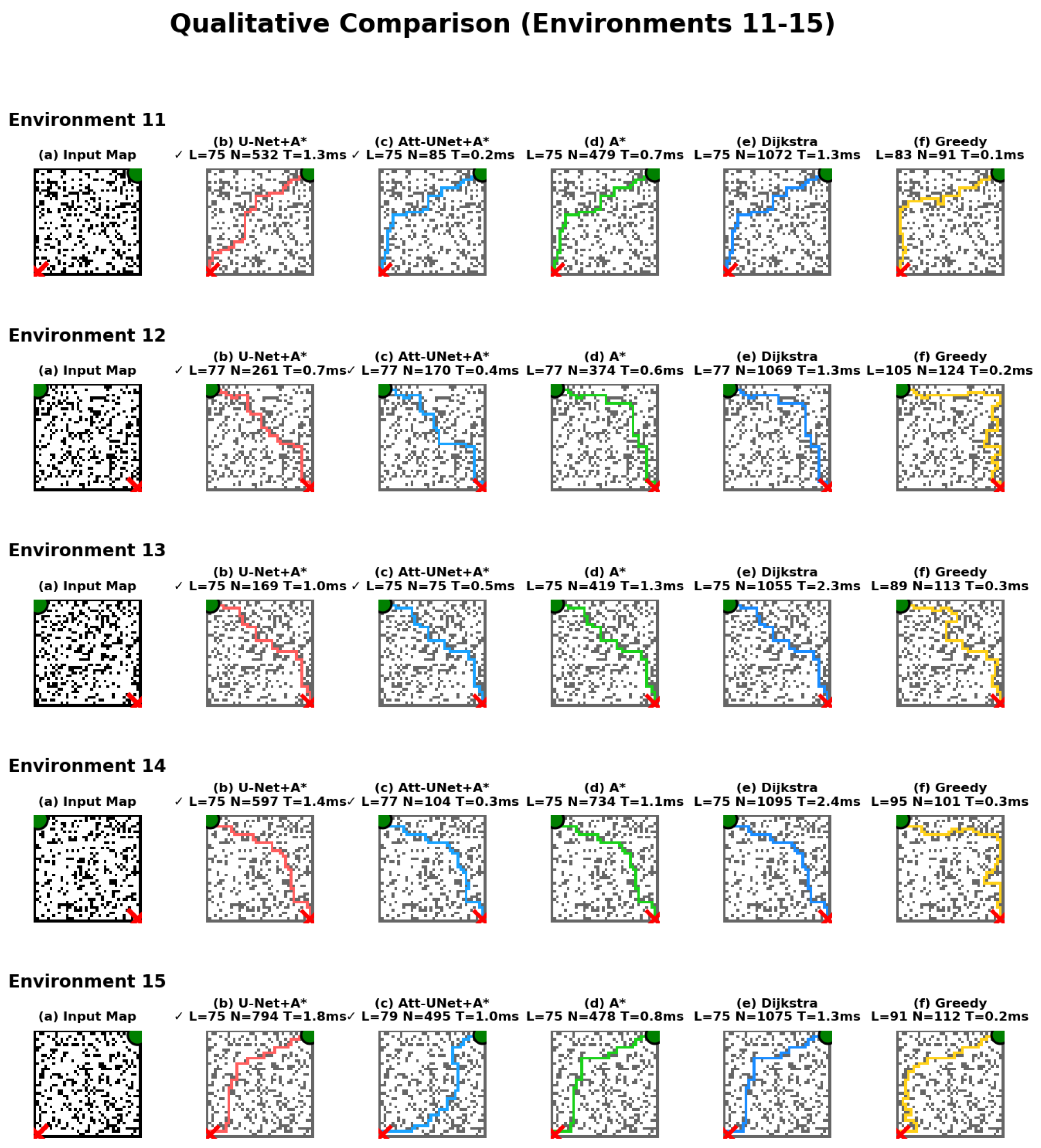
Figure A4.
Environments 16–20. For each environment row, the columns represent: (a) Input Map; (b) U-Net + A* (red path); (c) Attention U-Net + A* (blue path); (d) A* (green path); (e) Dijkstra (cyan path); (f) Greedy (yellow path). The green circles denote the start positions and the red stars indicate the goals. The check mark (✓) indicates that the algorithm successfully found an optimal path.
References
- Tang, Y.; Zakaria, M.A.; Younas, M. Path Planning Trends for Autonomous Mobile Robot Navigation: A Review. Sensors 2025, 25, 1206. [Google Scholar] [CrossRef] [Scilit]
- Waga, A.; Benhlima, S.; Bekri, A.; Abdouni, J.; Saber, F.Z. A survey on autonomous navigation for mobile robots: From traditional techniques to deep learning and large language models. J. King Saud Univ. Comput. Inf. Sci. 2025, 37, 198. [Google Scholar] [CrossRef] [Scilit]
- Regragui, A.; Benhlima, S.; Bekri, A. Vis-To-Nav: Visual Autonomous Navigation for Mobile Robots with a Limited Field of View. In Proceedings of the Intersection of Artificial Intelligence, Data Science, and Cutting-Edge Technologies: From Concepts to Applications in Smart Environment, Errachidia, Morocco, 7–9 November 2024; Farhaoui, Y., Herawan, T., Lucky Imoize, A., Allaoui, A.E., Eds.; Springer: Cham, Switzerland, 2025; pp. 196–201. [Google Scholar]
- Waga, A.; Benhlima, S.; Bekri, A. Enhanced autonomous driving. In Advances in Computational Intelligence and Robotics; IGI Global: Palmdale, PA, USA, 2025; pp. 237–260. [Google Scholar]
- Hart, P.E.; Nilsson, N.J.; Raphael, B. A Formal Basis for the Heuristic Determination of Minimum Cost Paths. IEEE Trans. Syst. Sci. Cybern. 1968, 4, 100–107. [Google Scholar] [CrossRef] [Scilit]
- Dijkstra, E.W. A note on two problems in connexion with graphs. Numer. Math. 1959, 1, 269–271. [Google Scholar] [CrossRef] [Scilit]
- Waga, A.; Benhouria, Y.; Ba-Ichou, A.; Benhlima, S.; Bekri, A.; Abdouni, J. A New Method for Mobile Robots to Learn an Optimal Policy from an Expert Using Deep Imitation Learning. In Proceedings of the Digital Technologies and Applications, Fez, Morocco, 27–28 January 2023; Motahhir, S., Bossoufi, B., Eds.; Springer: Cham, Switzerland, 2023; pp. 873–882. [Google Scholar]
- Wang, W.; Wu, Z.; Luo, H.; Zhang, B. Path Planning Method of Mobile Robot Using Improved Deep Reinforcement Learning. J. Electr. Comput. Eng. 2022, 2022, 5433988. [Google Scholar] [CrossRef] [Scilit]
- Ji, Y.; Sun, R.; Wang, Y.; Zhu, Z.; Liu, Z. Dynamic Path Planning for Unmanned Autonomous Vehicles Based on CAS-UNet and Graph Neural Networks. Sensors 2025, 25, 4283. [Google Scholar] [CrossRef] [Scilit] [PubMed]
- Kabir, R.; Watanobe, Y.; Islam, M.R.; Naruse, K. Enhanced Robot Motion Block of A-Star Algorithm for Robotic Path Planning. Sensors 2024, 24, 1422. [Google Scholar] [CrossRef] [Scilit]
- Yin, C.; Tan, C.; Wang, C.; Shen, F. An Improved A-Star Path Planning Algorithm Based on Mobile Robots in Medical Testing Laboratories. Sensors 2024, 24, 1784. [Google Scholar] [CrossRef] [Scilit]
- Duchoň, F.; Babinec, A.; Kajan, M.; Beňo, P.; Florek, M.; Fico, T.; Jurišica, L. Path planning with modified A star algorithm for a mobile robot. Procedia Eng. 2014, 96, 59–69. [Google Scholar] [CrossRef] [Scilit]
- Fan, J.; Chen, X.; Liang, X. UAV trajectory planning based on bi-directional APF-RRT* algorithm with goal-biased. Expert Syst. Appl. 2023, 213, 119137. [Google Scholar] [CrossRef] [Scilit]
- Guo, S.; Gong, J.; Shen, H.; Yuan, L.; Wei, W.; Long, Y. DBVSB-P-RRT*: A path planning algorithm for mobile robot with high environmental adaptability and ultra-high speed planning. Expert Syst. Appl. 2025, 266, 126123. [Google Scholar] [CrossRef] [Scilit]
- Dong, X.; Wang, Y.; Fang, C.; Ran, K.; Liu, G. FHQ-RRT*: An Improved Path Planning Algorithm for Mobile Robots to Acquire High-Quality Paths Faster. Sensors 2025, 25, 2189. [Google Scholar] [CrossRef] [Scilit]
- Zhu, L.; Duan, P.; Meng, L.; Yang, X. GAO-RRT*: A path planning algorithm for mobile robot with low path cost and fast convergence. AIMS Math. 2024, 9, 12011–12042. [Google Scholar] [CrossRef] [Scilit]
- Zhang, Y.; Cui, C.; Zhao, Q. Path Planning of Mobile Robot Based on A Star Algorithm Combining DQN and DWA in Complex Environment. Appl. Sci. 2025, 15, 4367. [Google Scholar] [CrossRef] [Scilit]
- Song, Q.; Li, S.; Yang, J.; Bai, Q.; Hu, J.; Zhang, X.; Zhang, A. Intelligent Optimization Algorithm-Based Path Planning for a Mobile Robot. Comput. Intell. Neurosci. 2021, 2021, 8025730. [Google Scholar] [CrossRef] [Scilit] [PubMed]
- Liu, M.; Zhang, H.; Yang, J.; Zhang, T.; Zhang, C.; Bo, L. A path planning algorithm for three-dimensional collision avoidance based on potential field and B-spline boundary curve. Aerosp. Sci. Technol. 2024, 144, 108763. [Google Scholar] [CrossRef] [Scilit]
- Menon, A.S.; Damm, E.R.; Howard, T.M. Homotopy-Aware Efficiently Adaptive State Lattices for Mobile Robot Motion Planning in Cluttered Environments. IEEE Robot. Autom. Lett. 2025, 10, 947–954. [Google Scholar] [CrossRef] [Scilit]
- Li, N.; Gao, Z.; Ouyang, Y.; Zeng, Y. Obstacle-Avoiding Path Planning for Robotic Manipulators Based on Recursive Segmentation Point Migration Optimization and Progressive Inverse Kinematics. IEEE Trans. Autom. Sci. Eng. 2025, 22, 20876–20890. [Google Scholar] [CrossRef] [Scilit]
- Zhang, D.; Gai, Y.; Ju, R.; Zhou, M.; Cao, Z. A Cosine Similarity Based Multitarget Path Planning Algorithm for Cable-Driven Manipulators. IEEE/ASME Trans. Mechatron. 2025, 30, 2379–2388. [Google Scholar] [CrossRef] [Scilit]
- Hu, B.; Cao, Z.; Zhou, M. An Efficient RRT-Based Framework for Planning Short and Smooth Wheeled Robot Motion Under Kinodynamic Constraints. IEEE Trans. Ind. Electron. 2021, 68, 3292–3302. [Google Scholar] [CrossRef] [Scilit]
- Lei, X.; Zhang, Z.; Dong, P. Dynamic Path Planning of Unknown Environment Based on Deep Reinforcement Learning. J. Robot. 2018, 2018, 5781591. [Google Scholar] [CrossRef] [Scilit]
- Zhang, Z.; Fu, H.; Yang, J.; Lin, Y. Deep reinforcement learning for path planning of autonomous mobile robots in complicated environments. Complex Intell. Syst. 2025, 11, 277. [Google Scholar] [CrossRef] [Scilit]
- Jaramillo-Martínez, R.; Chavero-Navarrete, E.; Ibarra-Pérez, T. Reinforcement-Learning-Based Path Planning: A Reward Function Strategy. Appl. Sci. 2024, 14, 7654. [Google Scholar] [CrossRef] [Scilit]
- Chehelgami, S.; Ashtari, E.; Basiri, M.A.; Masouleh, M.T.; Kalhor, A. Safe deep learning-based global path planning using a fast collision-free path generator. Robot. Auton. Syst. 2023, 163, 104384. [Google Scholar] [CrossRef] [Scilit]
- Waga, A.; Ba-ichou, A.; Benhlima, S.; Bekri, A.; Abdouni, J. Efficient autonomous navigation for mobile robots using machine learning. IAES Int. J. Artif. Intell. 2024, 13, 3061–3071. [Google Scholar] [CrossRef] [Scilit]
- Diao, Z.; Guo, P.; Zhang, B.; Zhang, D.; Yan, J.; He, Z.; Zhao, S.; Zhao, C.; Zhang, J. Navigation line extraction algorithm for corn spraying robot based on improved YOLOv8s network. Comput. Electron. Agric. 2023, 212, 108049. [Google Scholar] [CrossRef] [Scilit]
- Waga, A.; Benhlima, S.; Bekri, A.; Saber, F.Z.; Abdouni, J.; Mzili, T.; Regragui, A. Waypoint-guided trajectory planning for mobile robots using GPT-4o mini and ensemble learning-based action prediction. Array 2026, 29, 100636. [Google Scholar] [CrossRef] [Scilit]
- Ronneberger, O.; Fischer, P.; Brox, T. U-Net: Convolutional Networks for Biomedical Image Segmentation. arXiv 2015, arXiv:1505.04597. [Google Scholar] [CrossRef] [Scilit]
- Oktay, O.; Schlemper, J.; Folgoc, L.L.; Lee, M.C.H.; Heinrich, M.P.; Misawa, K.; Mori, K.; McDonagh, S.G.; Hammerla, N.Y.; Kainz, B.; et al. Attention U-Net: Learning Where to Look for the Pancreas. arXiv 2018, arXiv:1804.03999. [Google Scholar] [CrossRef] [Scilit]
- Ruby, U.; Yendapalli, V. Binary cross entropy with deep learning technique for Image classification. Int. J. Adv. Trends Comput. Sci. Eng. 2020, 9, 5393–5397. [Google Scholar] [CrossRef] [Scilit]
- Lin, T.; Goyal, P.; Girshick, R.B.; He, K.; Dollár, P. Focal Loss for Dense Object Detection. arXiv 2017, arXiv:1708.02002. [Google Scholar] [CrossRef] [Scilit]
- Kingma, D.P.; Ba, J. Adam: A Method for Stochastic Optimization. arXiv 2017, arXiv:1412.6980. [Google Scholar] [CrossRef] [Scilit]

Disclaimer/Publisher’s Note: The statements, opinions and data contained in all publications are solely those of the individual author(s) and contributor(s) and not of MDPI and/or the editor(s). MDPI and/or the editor(s) disclaim responsibility for any injury to people or property resulting from any ideas, methods, instructions or products referred to in the content. |
© 2026 by the authors. Licensee MDPI, Basel, Switzerland. This article is an open access article distributed under the terms and conditions of the Creative Commons Attribution (CC BY) license.