


Abstract
Construction and demolition waste (CDW) sorting on conveyors requires robots to intercept irregular targets while maintaining alignment under motion constraints. However, CDW research has emphasised perception, grasp generation, and planned trajectory execution, with limited evidence linking reactive velocity control to sorting productivity. This study formulates a control-oriented evaluation framework to characterise target tracking and examine whether conveyor motion compensation improves acquisition and recovery as conveyor speed increases. A Unity–ROS 2 digital twin using data-derived CDW objects and a UR10e manipulator compared feedback (FB) and combined feedforward and feedback (FF+FB) velocity control across three independently seeded 600 s simulation runs per operating condition. FF+FB maintained progressive tracking convergence across conveyor speeds of 0.4–0.6 m/s. At 0.5 m/s, FF+FB increased the mean pick completion rate from 40.8% to 78.1% and recovery throughput from 4.43 to 6.77 objects/min relative to FB. At 0.6 m/s, pick completion increased from 23.0% to 91.7%, while throughput increased from 2.37 to 6.63 objects/min. Despite lower Approach completion rates, FF+FB consistently achieved stronger downstream acquisition and recovery performance. Comparable cycle durations at 0.5 m/s showed that productivity gains arose from successful acquisition and transfer rather than faster cycles. Repeated seed evaluation demonstrated substantial performance differences between the controllers, although the limited number of independent runs constrains formal statistical inference. By linking motion demand and stage outcomes to throughput, the framework shows how reactive moving target control influences CDW sorting productivity across conveyor speeds.
1. Introduction
Construction and demolition waste (CDW) streams contain heterogeneous materials with irregular shapes, sizes, surface conditions, and spatial arrangements, making selective recovery substantially more difficult than handling structured industrial parts [1]. Effective material recovery is important for the transition towards a circular economy, where waste materials are returned to productive use through reuse and recycling rather than being discarded. The environmental benefits of this transition depend not only on improving recovery and recycling rates but also on system conditions that influence associated carbon savings [2]. Although manual sorting remains common, it is labour intensive, difficult to scale, and can expose workers to dust, sharp objects, heavy fragments, and other hazards. Consequently, artificial intelligence (AI) and robotic automation are receiving increasing attention as means of improving material identification, recovery efficiency, and worker safety in CDW management. Recent reviews indicate that research is moving beyond image-based recognition toward integrated robotic sorting systems capable of converting perception outputs into physical material handling actions [3]. A recent systematic mapping review further identified persistent gaps in operational validation, integrated robotic handling, and physical separation, highlighting the need to connect technical developments with measurable sorting outcomes [4].
Recent CDW robotics reflects this transition from identifying waste to determining and executing robotic actions. Wang et al. [5] developed a vision-based robotic prototype using instance segmentation to identify and pick irregular CDW objects. Chen et al. [6] further combined waste recognition with a three-dimensional (3D) object pickup strategy in an autonomous construction site sorting robot. More recently, Prasad and Arashpour [7] introduced the ReCoDeWaste red-green-blue-depth (RGB-D) dataset and a boundary-guided grasp detection method for highly cluttered CDW streams. These developments have substantially advanced object localisation and grasp generation. However, obtaining a valid target or grasp pose does not ensure successful conveyor sorting when the object continues to move while the manipulator approaches it.
Dynamic interception introduces a distinct control requirement because the target position changes continuously during robot motion. The manipulator must reduce tracking error while responding to target velocity and operating within finite joint, workspace, and timing constraints. Moving target control is well established outside the CDW domain. González Huarte and Ibarguren [8] demonstrated that target motion influences positioning error, task completion time, and success in position-based visual servoing, while velocity feedforward (FF) and closed-loop velocity control have been used to improve real-time interception of moving objects [9,10]. Within CDW robotics, however, manipulation research has predominantly emphasised grasp pose generation, motion planning, scheduling, and planned trajectory execution [5,6,11,12]. Comparatively less attention has been given to reactive velocity-level control of moving CDW targets and to how its tracking behaviour propagates to acquisition and sorting productivity.
RaapWaste represents an important step towards system-level CDW manipulation by integrating grasp evaluation, scheduling, motion planning, simulation, and physical validation and reporting sorting throughput and sorting ratio [12]. Its execution remains based on planned trajectories forwarded to the robot controller, leaving reactive control during execution as a separate challenge. This distinction motivates evaluation not only of whether a target can be planned for, but whether closed-loop control can maintain sufficient alignment with an irregular object as it travels through the interception region. To investigate this relationship under repeatable conditions, our previous work introduced a data-derived digital twin framework that converts red–green–blue (RGB) annotations of real CDW scenes into lightweight 3D assets and reproduces them in a Unity conveyor environment coupled with robot operating system 2 (ROS 2) [13]. That study focused on environment generation and computational validation. The present study uses the resulting environment as an experimental platform for control evaluation, with pre-generated target information held fixed so that controller behaviour can be examined independently of perception uncertainty.
This study investigates how conveyor motion compensation influences dynamic interception and sorting performance for irregular CDW targets. It examines whether incorporating target velocity into reactive velocity control improves progression from target tracking to acquisition and recovery, how this behaviour changes with conveyor speed, and how controller-level performance translates into system-level productivity. Using a UR10e manipulator, feedback (FB) and combined feedforward and feedback (FF+FB) control are compared at conveyor speeds of 0.5 and 0.6 m/s, with FF+FB additionally evaluated at 0.4 m/s. The study makes three contributions: (1) a control-oriented evaluation methodology linking moving target tracking with stage-level task outcomes and measured recovery productivity in a data-derived CDW environment; (2) application and systematic evaluation of constrained velocity-level FB and FF+FB control for interception of irregular moving CDW targets; and (3) multilevel performance characterisation connecting tracking convergence, task progression, cycle execution, and robot velocity demand with system-level recovery throughput.
2. Related Work
2.1. AI and Robotic Manipulation for CDW Sorting
Research on automated CDW sorting has progressively moved from material recognition toward spatial localisation and action-oriented perception. Earlier deep learning (DL) studies demonstrated the feasibility of image-level CDW classification [14,15], while semantic segmentation enabled pixel-level estimation of material composition within mixed waste scenes [16]. Object detection subsequently improved localisation of individual recyclable items, although degradation under stacking and adherence highlighted the difficulty of transferring models from isolated objects to realistic waste streams [17]. The introduction of benchmark datasets such as CODD further supported both object detection and instance segmentation for automated CDW sorting [18].
More recent studies have focused on the practical challenges encountered in real CDW streams, including limited annotations, clutter, overlapping objects, and irregular material appearance. Semi-supervised segmentation has been investigated to reduce dependence on extensive manual annotations [19], prompt-guided segmentation has supported interactive recognition in clutter [20], and RGB-D approaches have incorporated geometric information to improve separation of overlapping objects [21]. Despite these advances, deformation, contamination, scale variation, occlusion, and severe clutter continue to affect instance segmentation performance [22]. Shape-aware segmentation has subsequently been introduced to improve both mask and boundary quality for irregular recyclables [23], while dedicated datasets have increasingly sought to represent class-wise segmentation under realistic clutter [24].
The progression toward robotic action is particularly evident in recent grasp-oriented research. Prasad and Arashpour [7] combined RGB-D information with boundary-guided grasp prediction for cluttered CDW, while Deng et al. [11] integrated detection, spatial localisation, grasp estimation, and robotic execution. Similar developments in other waste domains increasingly combine recognition, conveyor tracking, and manipulation [25,26,27,28]. Importantly, these studies show that accurate perception and grasp localisation constitute only part of the sorting problem; mechanical execution can remain limiting even when recognition performance is high [25]. Therefore, for moving conveyor targets, identifying a valid grasp pose is not sufficient by itself. The manipulator must also reach the target and maintain sufficient alignment within the available workspace and interception time. This motivates treating moving target control as a separate problem from perception and grasp generation in the present evaluation.
2.2. Robotic Planning and Control for Moving Object Sorting
Tracking and intercepting moving targets have been studied extensively outside the CDW domain. A common strategy combines FB correction with prediction or FF compensation for target motion. Wang et al. [10] incorporated predicted target velocity as a FF term within visual servo control, while Chen et al. [9] combined estimated velocity FF with refined proportional-integral-derivative (PID) FB for moving object capture and placement. In the latter system, the manipulator operates in velocity control mode so that motion can be updated continuously during interception. Adaptive approaches have also used reinforcement learning to tune visual servo control [29], while dynamic target capture has been addressed through online configuration space planning [30]. Robust control has also been investigated in robotic systems subject to actuation and environmental uncertainties. Chen et al. [31] investigated robust motor control for legged lunar robots, while a subsequent study considered robust control of robotic leg dynamics [32]. Related approaches addressed mechanical leg control [33] and leg–soil interactions under uncertain environmental conditions [34]. Although these studies address different robotic configurations and disturbance sources, they demonstrate complementary approaches to uncertainty-aware control beyond the scope of the present FB and FF+FB comparison.
Recent work has further investigated how interception timing, trajectory generation, and manipulator operating limits affect moving object manipulation. Flores Campos et al. [35] developed prescribed time interception for synchronising a manipulator with moving target trajectories. Other studies have estimated robotic task time to support real-time interception and scheduling of moving pick-and-place targets [36], quantified productivity gains arising from coordinated robotic motion [37], and investigated near time optimal online picking from moving conveyors [38]. More recently, Cao et al. [39] investigated vision-based reinforcement learning for grasping moving conveyor objects in simulation. At the production system level, Ladefoged et al. [40] examined how look-ahead information and multi-conveyor configurations influence robotic pick-and-place performance. Recent trajectory optimisation studies continue to examine the relationship between motion design, dynamic constraints, and handling performance [41]. These studies show that both planned interception and reactive velocity control are established approaches for structured moving object manipulation. The unresolved issue for the present application is how these control principles perform when the targets are irregular CDW objects and whether differences in control strategy translate into meaningful gains in sorting execution.
Current CDW manipulation systems remain primarily pose and trajectory oriented. Wang et al. [5] and Chen et al. [6] determine object location and pickup configurations for robotic collection, while more recent perception-to-action work similarly emphasises grasp localisation and execution [11]. RaapWaste [12] extends this substantially by integrating scheduling, grasp evaluation, trajectory planning, and system-level assessment for conveyor sorting. Its executor forwards the planned trajectories to the robot controller without modifying them during execution, while reactive execution is identified as an extension of the framework. Consequently, reactive velocity-level interception remains comparatively underexplored for CDW sorting, particularly when considered together with application-level outcomes. Accordingly, limited evidence connects closed-loop velocity tracking of irregular moving CDW targets with Approach completion, acquisition, cycle execution, and measured recovery productivity.
2.3. Simulation and Digital Twins for Robotic Control Evaluation
Simulation and digital twin environments provide a practical means of examining controller behaviour under repeatable target and operating conditions. ROS-integrated Unity environments have been used for monitoring and pick-and-place simulation of robotic manufacturing stations [42], while bidirectional Unity-ROS digital twins have been evaluated for communication and kinematic accuracy [43]. Digital twins have also been used to test manipulator control strategies before physical implementation [44].
Comparative studies of Unity and Gazebo have identified complementary strengths in real-time responsiveness, visual fidelity, physics modelling, and ROS integration [45]. Unity–ROS architectures have subsequently been extended to robot path planning and hardware execution [46], while digital twin platforms have been used to implement and evaluate manipulator control algorithms before transferring related control logic to physical systems [47]. These studies establish simulation as a repeatable environment for manipulating operating conditions and examining control behaviour before physical deployment.
Within CDW sorting, our previous work [13] established an RGB-derived Unity–ROS 2 environment in which annotations from real waste images are converted into lightweight 3D assets. The present study uses this environment to investigate reactive velocity control rather than environment generation or perception performance. Target information is treated as known, allowing FB and FF+FB control to be evaluated as conveyor speed changes while retaining irregular data-derived object geometry. Therefore, the literature connects three relevant areas: CDW perception and manipulation, moving target robotic control, and simulation-based control evaluation. Their intersection remains comparatively limited, particularly for velocity-level interception of irregular CDW objects and the relationship between such control and downstream sorting productivity. This motivates the multilevel evaluation framework used in the present study.
3. Methodology
3.1. Control-Oriented Evaluation Framework
The methodology evaluates how moving target control propagates from end effector tracking to application-level CDW sorting outcomes. Figure 1 illustrates the overall workflow. RGB images and corresponding instance annotations are used offline to generate lightweight 3D CDW assets using the data-driven reconstruction procedure developed in our previous work [13]. The resulting objects are spawned on a moving conveyor within Unity and tracked as they pass through the robotic sorting workspace. Unity continuously supplies the current target state to the ROS 2 control system. This communication represents the target state information that would be provided in a physical sorting system by object detection and conveyor tracking, where belt motion can be measured using an encoder to update the target position as it moves along the conveyor. The controller generates task space commands using either FB control or FF+FB control and maps them to UR10e joint velocities through a constrained quadratic program (QP).
Figure 1.
Control-oriented evaluation workflow for conveyor-based CDW sorting.
Performance is evaluated at three connected levels: tracking behaviour during interception, progression through the pick-and-place sequence, and final recovery productivity. Perception uncertainty is intentionally excluded from the experiments by treating object identity and target position, velocity, and orientation as known inputs, while detailed grasp mechanics are abstracted using the geometric acquisition criterion described in Section 3.6. This controlled setup allows the effects of FB and FF+FB velocity control to be compared independently of perception errors, while retaining irregular data-derived target geometry.
3.2. Data-Derived CDW Simulation Environment
The simulated waste stream was constructed using RGB images and instance annotations obtained from the CDW dataset employed in [13]. For each annotated waste instance, the 2D object contour was converted into a lightweight 3D mesh using the previously established reconstruction pipeline. Because depth information was unavailable for the RGB images, object thickness was assigned using predefined height assumptions appropriate to the corresponding waste representation. The reconstruction procedure is detailed in [13] and is not repeated here.
For the present study, these assets were used as irregular robotic targets rather than idealised primitive geometries, retaining image-derived variations in object footprint and shape while remaining computationally suitable for repeated control experiments. During each test, waste assets were spawned on the conveyor and translated at the prescribed belt velocity vb, with the conveyor width set to 0.90 m. To introduce variability in conveyor motion, a time varying speed perturbation bounded within ±0.02 m/s was applied to the nominal conveyor speed across all operating conditions. This represents fluctuations in conveyor motion rather than uncertainty in the perceived target state. No online segmentation or classification model was executed during the experiments. The object identity and state were supplied directly to the control pipeline as defined in Section 3.1.
3.3. Robotic Sorting Cell and ROS 2–Unity Integration
The virtual sorting cell consisted of a moving conveyor, a six-axis UR10e manipulator (Universal Robots A/S, Odense, Denmark) equipped with a Robotiq 2F-140 adaptive two-finger gripper (Robotiq Inc., Lévis, QC, Canada), and sorting bins positioned within the robot workspace. The UR10e has a nominal reach of 1.3 m and a rated payload of 12.5 kg, while the Robotiq 2F-140 provides a maximum finger stroke of 140 mm and a rated grasp force of 10–125 N. These specifications describe the robotic hardware represented in the simulation. However, physical grasp forces were not modelled, as detailed in Section 3.6. As shown in Figure 2, the system extends our previous UR5e-based simulation framework [13] by using the longer reach UR10e manipulator, providing the workspace required for the 0.90 m conveyor used in the present experiments.
Figure 2.
Unity robotic CDW sorting environment: (a) virtual sorting cell comprising the UR10e manipulator, moving conveyor, sorting bins, and data-derived waste objects, with red callouts illustrating examples of simulated waste objects corresponding to regions in the source RGB image; and (b) representative screenshots from the simulated sorting experiments, showing additional workspace views and the UR10e manipulator with the Robotiq 2F-140 gripper during operation.
The robot was represented in Unity using articulated joints corresponding to the manipulator kinematic chain. The virtual gripper was attached to the manipulator tool frame, with geometric contact detection used to evaluate target acquisition as described in Section 3.6. Robot state and target information were exchanged with the ROS 2 controller through the ROS-Unity transmission control protocol (TCP) interface. At each control iteration, the ROS 2 node received the current joint configuration (six joint positions), denoted by q, and used it to update the MoveIt robot state, from which the current end effector pose was calculated. The target position, translational velocity, and orientation were supplied from Unity as controller inputs. The controller then computed the joint velocity command, denoted by , which was published to the forward velocity controller for execution by the simulated UR10e.
3.4. Velocity Control Formulation
3.4.1. Moving Target Task Space Control
Let pt(t), and pe(t) denote the current Cartesian target supplied to the controller and the current end effector position, respectively. The components of pt are denoted by xt, yt, and zt. The state dependent Cartesian goal supplied to the controller is defined as:
where hh is the configured hover offset (representing tool0 to TCP offset) and zplane is the minimum allowable end effector height. Before the tracking command is calculated, pg is processed by a geometric safety routine that may generate an intermediate target pd when direct motion towards the goal would pass through the keep-out region surrounding the robot base:
where S(∙) denotes the safe target function described in Appendix A.1.
For FB control, the commanded translational velocity before saturation is generated from the instantaneous tracking error as:
where kp is the translational FB gain. FF+FB control additionally incorporates the supplied target velocity
where gff is the FF gain, vt is the target translational velocity expressed in the robot base frame, and d is the distance from the end effector to the actual target goal. The factor progressively activates the FF contribution as the end effector approaches the target. It is zero outside the FF activation distance ds, increases smoothly between ds and the full FF distance df, and becomes one at or within df. The exact activation function is given in Appendix A.2. The activation distances ds = 0.25 m and df = 0.08 m were selected empirically during controller development rather than derived analytically. This distance-dependent activation was introduced to reduce undesirable motion caused by premature FF compensation, particularly when the end effector is positioned downstream of the selected target, where the FF contribution may oppose the FB correction required to approach the target. These parameters were kept fixed across all experimental conditions. Thus, FB responds to position error alone, whereas FF+FB additionally compensates for target motion during convergence. The raw translational command is limited to the configured maximum Cartesian speed vmax, and the resulting command is denoted by vd. The velocity saturation procedure is also provided in Appendix A.2.
Tool orientation is regulated simultaneously using proportional rotational feedback. The desired orientation Rd is constructed from the target orientation angle , while Re denotes the current end effector orientation. These quantities are used with the rotational FB gain kr to obtain the angular velocity command . The construction of Rd and the rotational error formulation are provided in Appendix A.3. The resulting desired Cartesian twist is
3.4.2. Quadratic Programming Joint Velocity Controller
The desired Cartesian twist is mapped to joint velocity using a constrained QP, where the objective balances Cartesian tracking, joint velocity regularisation, and null space posture restoration. Let denote the geometric Jacobian of the UR10e at joint configuration q. The commanded joint velocity is obtained from
subject to
where is the joint velocity regularisation coefficient, wp is the weight assigned to posture restoration, N is the damped task null space projector, and vp is the posture restoration velocity. The construction of N using the damped pseudoinverse of the Jacobian and the calculation of vp are described in Appendix A.4.
In Equation (7), A(q) denotes the constraint matrix, while l(q) and u(q) contain the corresponding lower and upper bounds. These constraints regulate end effector vertical clearance, forearm clearance, self-collision avoidance, and joint position and velocity limits. Their complete formulations are provided in Appendix A.5. The QP is solved online using operator splitting QP (OSQP) with warm starting. Details of the solver implementation and the emergency self-collision response are provided in Appendix A.6. The definitions and values of all controller and safety parameters are summarised in Appendix A.7.
3.5. Pick-and-Place State Machine
Task execution was coordinated by a ROS 2 state machine operating at 20 Hz. The sequence comprised seven states: Idle → Approach → Lower → Grip → Raise → Place → Release. In Idle, the manipulator remained at its safe pose until an eligible target was selected. The selected object ID was then locked for the attempt, and its position, orientation, and conveyor velocity were transformed from Unity into the ROS base frame. Figure 3 illustrates the state sequence and principal recovery transitions.
Figure 3.
State machine for conveyor-based target acquisition and sorting, showing the normal execution sequence and principal recovery transitions.
During Approach, the end effector tracked the moving target at the configured approach height with conveyor velocity supplied as target velocity. Once the planar error remained within tolerance for the required hold period, Lower was entered and planar tracking continued while the tool descended. Grip began when the planar and vertical tolerances were satisfied, and moving target tracking remained active during acquisition. The Grip state terminated upon successful acquisition confirmation or when the maximum interval of 1.0 s was reached, whichever occurred first, and was followed by Raise regardless of the acquisition outcome. Following successful acquisition, the object proceeded to Place after reaching the transport height; following an unsuccessful acquisition, Raise acted as a retraction motion before the system returned to Idle for recovery. During Raise, the planar target was fixed at its acquisition position while the tool moved to the transport height, and conveyor compensation was disabled. The object was then transported to its assigned bin during Place and detached during Release. Completion or recovery cleared the target lock and returned the system to Idle. Detailed transition criteria and executor parameters are provided in Appendix B.
3.6. Geometric Target Acquisition Abstraction
Detailed contact mechanics were excluded because the study evaluated moving target control rather than physical grasp stability. Therefore, acquisition was represented using a geometric mechanism in Unity. Three trigger colliders were located at the tool centre point and two fingertips, and acquisition was considered successful only when all three simultaneously intersected the selected object. This criterion requires simultaneous geometric contact at three locations rather than incidental contact, without evaluating the forces required for grasp stability. Following successful acquisition, the object was made kinematic and attached to the gripper while preserving its pose, allowing it to follow the manipulator through Raise and Place. During Release, it was detached and returned to dynamic simulation, allowing it to fall into the assigned bin, where a bin trigger confirmed successful recovery. Accordingly, reported pick and recovery outcomes represent geometric target acquisition and task execution rather than physical grasp stability. Because frictional slip, unstable contact, and object tipping are not explicitly modelled, the geometric acquisition abstraction may overestimate physically achievable recovery performance. The potential influence of these unmodelled grasp failures on comparative controller performance is therefore examined through a sensitivity analysis using hypothetical grasp retention probabilities in Section 4.2.
3.7. Target Prioritisation and Selection
Tracked waste objects were assigned priority scores according to class and position along the conveyor. For object i, the priority score used in the experiments can be expressed as
where zi is the object position along the conveyor axis, zr is the robot reference position, wc,i is the weight associated with object class i, and controls the spatial decay of the priority. Here, zi, zr, zL, and zU are expressed in the Unity coordinate frame, in which the z axis corresponds to the conveyor direction; this differs from the ROS base frame used in Section 3.4, where z denotes the vertical axis. The active region was bounded by zL = −0.2 m and zU = 1.0 m, with zr = 1.0 m and . Class weights were 0.7 for concrete and brick and 0.6 for wood and rubber. Consequently, priority increased as an object approached the robot reference position, with a small class-dependent preference incorporated through wc,i. At the start of each pick attempt, the highest-priority candidate was selected and its ID locked. Subsequent position and orientation updates were matched using this ID so that the manipulator continued to track the same object throughout the attempt rather than switching to another candidate as priorities changed.
3.8. Experimental Conditions and Evaluation Metrics
Each operating condition was evaluated over three independently seeded simulation runs, with an analysis duration Ttest = 600 s per run. FF+FB control was tested at conveyor speeds of 0.4, 0.5, and 0.6 m/s, whereas FB control was evaluated at 0.5 and 0.6 m/s, resulting in 15 experimental runs. At each common conveyor speed, matched random seeds were used for FB and FF+FB to generate comparable incoming object sequences. Different seeds introduced variation in object selection, geometry, spatial distribution, and arrival patterns, while conveyor speed and controller parameters were held constant within each operating condition. To establish a consistent observation window, the analysis was initiated at the recorded spawning event of a predefined object ID (used ID 25). Only engagements targeting this object or subsequently spawned objects were considered, and attempts that remained incomplete at the end of the 600 s interval were excluded from completed attempt statistics.
Controller-level tracking performance was quantified using the planar error between the moving target and end effector,
where xt and xe are the target and end effector coordinates in the conveyor plane. To examine convergence rather than only the final error, the Approach state was divided into four equal normalised temporal intervals and exy was also evaluated during Lower. For each seed, the mean planar error was calculated within each interval of an individual engagement and subsequently averaged across qualifying engagements. The final results were expressed as mean ± standard deviation across the three seed-level means. This trajectory-level analysis was performed for FF+FB engagements that successfully completed Approach and entered Lower, regardless of subsequent acquisition success. A separate single-seed ablation was conducted under FF+FB control at 0.5 m/s (seed 55), comparing the original posture weight wp = 0.5 against wp = 0, while maintaining the other controller and simulation parameters. For this comparison, mean planar tracking errors were calculated per object for target IDs observed in both runs during the corresponding Approach and Lower states, with orientation tracking error additionally evaluated during Lower.
System progression was evaluated using five event counts: NE, the number of eligible objects available for selection; NT, the number selected for a pick attempt; NL, the number that successfully progressed to Lower; NP, the number successfully acquired; and NR, the number successfully recovered in the assigned bin. The corresponding stage and overall success rates were
Here, , , , , and represent targeting rate (how many eligible objects were selected), Approach completion rate (whether a selected target was reached sufficiently to enter Lower), pick completion rate (successful acquisition after reaching Lower), transfer success rate (successful recovery after acquisition), and overall recovery rate (overall sorting success relative to all eligible objects), respectively. These stage-specific measures allow losses caused by target selection, moving target tracking, acquisition, and transport to be distinguished. Eligible objects were defined as unique objects entering the predefined picking region within the strict observation window, irrespective of whether the robot selected them. Stage progression was determined from actual ROS 2 executor state transition events, while acquisition and recovery were verified using the corresponding simulation events. The recorded object ID was used to associate each attempt with its selected target, and the terminal executor event provided the completion status and failure reason. Counts and rates were first calculated independently for each seed and subsequently summarised as mean ± standard deviation.
Execution efficiency was characterised using the duration of Approach, Lower, Grip, Raise, and Place for complete, successfully recovered cycles. State durations were obtained directly from the recorded executor transitions. For each seed, the mean duration of each state was calculated across successful cycles, and the three seed-level averages were subsequently summarised as mean ± standard deviation. The total cycle duration included the fixed Release interval of approximately 0.55 s, which was omitted from the individual state columns.
System productivity was represented by the measured recovery throughput,
where QR is expressed in objects/min. For the 600 s analysis window, QR = NR/10. This metric represents the number of successfully recovered objects associated with qualifying completed picking attempts within the 600 s analysis window rather than a capacity estimated from mean cycle time. Recovery throughput was calculated independently for each seed as the number of successfully recovered qualifying objects divided by the 10 min analysis duration. The reported throughput represents the mean ± standard deviation of these seed-level measurements. Unlike cycle time-derived capacity estimates, this measure incorporates losses resulting from unsuccessful target engagement, acquisition, and transfer.
Finally, robot velocity demand was characterised for the FF+FB condition at 0.5 m/s using the mean absolute joint velocity and end effector linear speed across successfully completed cycles. For a recorded speed quantity uk over M samples,
where for joint j, and for the end effector. For each seed, mean velocity magnitudes were calculated separately for each robot state. The reported mean and standard deviation were subsequently obtained from the three seed-level means, while the highest observed sampled velocity across all seeds was retained as the maximum. The recorded simulation data were post-processed using Python (version 3.10) scripts to obtain the reported evaluation metrics. OpenAI ChatGPT (GPT-6) was used to assist with drafting selected post-processing scripts, which were manually reviewed and verified by the authors before use in the analyses.
4. Results and Discussion
4.1. Moving Target Tracking Convergence
Figure 4 shows the mean planar tracking error during Approach and Lower for FF+FB control across three simulation seeds. At all three conveyor speeds, the mean tracking error decreased progressively through the four normalised Approach intervals, reaching its lowest value during Lower. At 0.4 m/s, the mean error decreased from 1.116 ± 0.054 m during the first Approach interval to 0.067 ± 0.001 m during Lower. Corresponding reductions from 0.954 ± 0.037 to 0.053 ± 0.002 m and from 0.484 ± 0.018 to 0.053 ± 0.003 m were observed at 0.5 and 0.6 m/s, respectively. The relatively small standard deviations between seeds, particularly towards the end of Approach and during Lower, indicate consistent tracking convergence across the evaluated randomised target sequences.
Figure 4.
Planar tracking error during Approach and Lower under FF+FB control at conveyor speeds of 0.4, 0.5, and 0.6 m/s. Approach is divided into four equal normalised temporal intervals, followed by Lower. Each cell represents the mean ± standard deviation across three simulation seeds. For each seed, tracking errors were first averaged within individual target engagements and then across engagements. Only complete engagements that successfully progressed from Approach to Lower were considered, irrespective of subsequent acquisition success.
The different initial errors across conveyor speeds should not be interpreted as evidence that higher conveyor speed inherently improves tracking. They partly reflect differences in the target conditions associated with the successful engagements included at each speed. Because targets are locked before reaching the manipulator, a faster conveyor may bring the selected object into the interception region more quickly, reducing the time or distance required to establish close tracking. However, the same increase in conveyor speed also shortens the available window for Lower and Grip. Thus, the key observation is that FF+FB maintained progressive tracking convergence across all tested conveyor speeds, with comparable final Lower tracking errors of approximately 0.05–0.07 m. This convergence was evaluated only for engagements that successfully progressed into Lower and therefore does not capture all unsuccessful tracking attempts. As shown subsequently by the stage progression results, the mean Approach completion rate decreased from 100.0% at 0.4 m/s to 55.3% at 0.6 m/s. Thus, the tracking heatmap and the stage progression analysis provide complementary information: the former characterises tracking convergence among successful Approaches, whereas the latter quantifies the proportion of engagements that achieve this progression.
To assess the influence of posture restoration on Cartesian tracking, an additional ablation compared FF+FB control at 0.5 m/s with wp = 0.5 and wp = 0, using seed 55. The comparison considered common object IDs across both runs, comprising 48 objects during Approach and 37 during Lower. With posture restoration enabled, the mean planar tracking error decreased from 0.611 to 0.538 m during Approach and from 0.0581 to 0.0499 m during Lower, corresponding to reductions of 11.9% and 14.2%, respectively. The mean orientation error during Lower increased slightly from 0.225° to 0.265°. These results indicate that the posture term has a measurable influence on Cartesian tracking rather than operating within an exactly decoupled null space. However, differences in engagement timing and the single-seed evaluation limit the generalisability of these findings.
4.2. Stage Progression and Recovery Productivity
Table 1 summarises stage progression and recovery performance across the three simulation seeds. At the common conveyor speed of 0.5 m/s, FB achieved a slightly higher mean Approach completion rate than FF+FB (88.5 ± 1.1% versus 86.1 ± 2.3%). However, this advantage did not persist during acquisition. FF+FB achieved a substantially higher pick completion rate of 78.1 ± 1.2%, compared with 40.8 ± 6.3% for FB. Transfer success remained high for both controllers, reaching 100.0 ± 0.0% for FF+FB and 99.2 ± 1.4% for FB. Consequently, the overall recovery rate increased from 8.8 ± 1.4% under FB to 13.3 ± 0.6% under FF+FB.
Table 1.
Stage progression and recovery performance under FF+FB and FB control across three simulation seeds, each evaluated over a 600 s analysis window.
At 0.6 m/s, the stage behaviour differed more strongly between the controllers. As also shown in Figure 5a, FB achieved a higher mean Approach completion rate than FF+FB (67.3 ± 8.2% versus 55.3 ± 0.4%). However, only 23.0 ± 14.4% of FB engagements reaching Lower resulted in successful acquisition, compared with 91.7 ± 1.6% under FF+FB. Transfer success remained high for both controllers, at 98.9 ± 1.9% for FB and 99.5 ± 0.9% for FF+FB. Consequently, FF+FB achieved an overall recovery rate of 7.8 ± 0.5%, compared with 2.8 ± 1.5% under FB. The greater variability observed for FB across the three simulation runs, particularly in pick completion and recovery, suggests less consistent downstream acquisition performance.
Figure 5.
Influence of conveyor speed on robotic sorting performance under FF+FB and FB control: (a) Approach completion rate and (b) measured recovery throughput over the 600 s analysis window. Markers indicate the mean across three simulation seeds, and error bars represent ±1 standard deviation. Each seed was evaluated over a strict 600 s analysis window.
To further explain these stage losses, recorded termination events were analysed across all operating conditions (counts aggregated across three seeds). At 0.4 m/s, FF+FB failures were mainly attributed to Grip interval expiry without successful acquisition (28 attempts). At 0.5 m/s, targets passing beyond the picking region accounted for most FF+FB failures (97), whereas FB failures were dominated by Grip interval expiry (152), followed by target passage (88). At 0.6 m/s, FF+FB failures occurred primarily when targets passed the picking region during Approach (176). In contrast, of the 343 FB attempts reaching Lower, only 72 achieved acquisition; 171 terminated during Lower (153 target passages, 17 timeouts, and one motion command rejection), while another 100 expired during Grip without successful acquisition. Of the 72 acquired objects, 71 were confirmed as successfully recovered within the observation window. These results identify target passage and unsuccessful acquisition within the permitted time as the principal causes of task losses, with their relative contributions varying across controller configurations and conveyor speeds.
Together, the stage progression and failure analysis results demonstrate that Approach completion alone is not sufficient to characterise moving target sorting performance. Reaching Lower indicates that the manipulator has converged sufficiently to progress beyond Approach, but successful acquisition still requires alignment to be maintained as the target continues to move through Lower and Grip. Under FF+FB, conveyor velocity compensation remained active through these states, which is consistent with the substantially higher pick completion observed at 0.6 m/s. Therefore, the higher Approach completion of FB at this speed should not be interpreted as superior overall control performance. The targeting rate provides a further example of why individual stage measures must be interpreted within the complete pipeline. At 0.6 m/s, FB achieved a higher mean targeting rate than FF+FB (19.7 ± 1.3% versus 15.5 ± 0.8%), yet produced substantially fewer recovered objects. This demonstrates that engaging a larger proportion of eligible objects does not necessarily improve recovery when subsequent acquisition remains unsuccessful.
The system-level consequences are shown in Figure 5b. FF+FB achieved mean recovery throughputs of 6.83 ± 0.06, 6.77 ± 0.12, and 6.63 ± 0.35 objects/min at conveyor speeds of 0.4, 0.5, and 0.6 m/s, respectively. By comparison, FB achieved 4.43 ± 0.42 objects/min at 0.5 m/s and 2.37 ± 1.27 objects/min at 0.6 m/s. Although Figure 5a indicates that Approach completion under FF+FB decreases as conveyor speed increases, recovery throughput remains comparatively stable across the same operating range. The mean number of eligible objects increased from 277.3 ± 29.9 at 0.4 m/s to 847.3 ± 21.2 at 0.6 m/s, whereas the mean number recovered remained approximately 67–69. This behaviour is consistent with the single manipulator approaching a cycle limited operating regime, where increasing target availability does not produce a proportional increase in sorting output. Consequently, the reduction in overall recovery rate with increasing conveyor speed does not correspond to an equivalent reduction in absolute recovery throughput.
To estimate the potential bias introduced by the geometric grasping abstraction, a sensitivity analysis was conducted by applying hypothetical grasp retention probabilities to the simulated recovery throughput. Assuming 80% grasp retention for both controllers, the adjusted throughputs remained higher for FF+FB than FB at 0.5 m/s (5.42 versus 3.54 objects/min) and 0.6 m/s (5.30 versus 1.90 objects/min). Under unequal grasp retention, the FF+FB throughput advantage would disappear if its retention probability fell below approximately 65% and 36% of that of FB at 0.5 and 0.6 m/s, respectively. These estimates illustrate the sensitivity of the observed advantage to unmodelled grasp failures rather than predicting physical grasp performance.
4.3. State Timing and Cycle Execution
Table 2 provides insight into how the stage progression translates into complete cycle execution. At 0.5 m/s, the mean total cycle durations were comparable for FF+FB and FB, at 6.73 ± 0.04 and 6.62 ± 0.15 s, respectively. Therefore, FF+FB did not achieve its higher recovery throughput by executing individual successful cycles faster. Instead, the productivity advantage arose primarily from a greater proportion of attempts progressing successfully through acquisition and recovery. At 0.6 m/s, FF+FB exhibited a lower mean total cycle duration of 5.92 ± 0.22 s, compared with 6.25 ± 0.09 s for FB. The largest state-level difference occurred during Lower, with mean durations of 0.60 ± 0.01 s for FF+FB and 1.25 ± 0.06 s for FB. The longer Lower duration under FB is consistent with the greater difficulty of maintaining alignment with the moving target during descent.
Table 2.
State and total cycle durations for successfully completed pick-and-place cycles under different control methods and conveyor speeds.
The state timing results indicate that Approach and Place account for much of the complete cycle duration. Under FF+FB, mean Approach duration decreased from 2.51 ± 0.16 s at 0.4 m/s to 0.82 ± 0.04 s at 0.6 m/s. This should not be interpreted as an intrinsic increase in robot speed. Instead, the difference may partly reflect changes in the interception geometry, because faster conveyor motion can bring selected targets closer to the manipulator during Approach. Similarly, Place duration varies with the acquisition location and assigned sorting bin. The repeated-seed analysis indicates that these timing patterns are relatively consistent across the evaluated target sequences, although individual cycle durations may exhibit greater variation than the seed-level averages suggest.
Place remained the longest state after acquisition, with mean durations of approximately 2.91–3.16 s across the evaluated conditions. This indicates that transporting the acquired object to its assigned destination accounts for a substantial portion of each successful cycle. Because the same placement logic was used for both controllers, however, the principal distinction between FB and FF+FB remains the ability to convert moving target engagements into successful recoveries. The observed mean Grip durations of 0.14–0.29 s were below the configured maximum interval of 1.0 s because the executor terminated acquisition early when successful object attachment was confirmed. The corresponding robot velocity demand is examined next to determine whether these cycle behaviours were achieved within the imposed motion limits.
4.4. Robot Velocity Demand
Table 3 characterises the joint and end effector velocity demand of FF+FB control at 0.5 m/s across three simulation seeds. Mean joint velocities remained below the configured limits, whereas higher peak velocities were observed during selected manipulation states. In particular, J6 reached approximately 2.51 rad/s during Approach, reaching its effective limit of 2.513 rad/s, while J2 reached approximately 100% during Raise. J4 reached approximately 2.20 rad/s during Raise, corresponding to 87.5% of its effective limit, while J1 reached approximately 1.47 rad/s during Lower, corresponding to 87.7% of its limit. These results demonstrate that joint velocity demand was concentrated in particular states and configurations, rather than remaining uniformly high throughout the complete manipulation cycle.
Table 3.
State-wise joint and end effector velocity demand for FF+FB control at a conveyor speed of 0.5 m/s across three simulation seeds.
The highest observed end effector linear speed was approximately 1.14 m/s during Raise, corresponding to 57.0% of the configured 2.0 m/s Cartesian velocity cap. This indicates that the Cartesian speed limit was not generally the dominant restriction under the analysed condition. Instead, individual joint limits became more influential for particular manipulator configurations, with J2 and J6 approaching their effective velocity limits, while J1 and J4 reached approximately 88% of their respective limits during selected states. At the same time, the relatively low mean velocities indicate that additional controller tuning could increase velocity utilisation during portions of the cycle where greater motion demand is beneficial. However, operating continuously near the allowable joint limits is not inherently required for successful task execution and may conflict with smooth tracking and the imposed QP constraints. Therefore, the controller parameters were tuned to provide stable and smooth motion and then kept fixed across the evaluated conditions, allowing the comparison to focus on the effect of FB versus FF+FB control rather than on condition specific speed optimisation.
Accordingly, the velocity results show that the implemented controller retained unused motion capacity during much of the cycle while approaching the configured joint velocity limits during selected transients. This distinction is important because unused average velocity capacity cannot be interpreted directly as unused sorting capacity. The overall performance also depends on target geometry, interception location, state transition criteria, and successful progression through the moving target acquisition sequence. Because the velocity analysis was performed for FF+FB at 0.5 m/s, these results characterise the motion demand and repeatability of the implemented controller rather than providing a direct comparison of velocity utilisation between FB and FF+FB.
4.5. System-Level Implications of Moving Target Control
The combined results show that moving target sorting performance cannot be adequately characterised using a single metric. Tracking convergence indicates whether the manipulator can approach a moving object, while stage progression determines whether this convergence is maintained sufficiently for acquisition and transfer. Cycle time describes successful executions, whereas recovery throughput also reflects attempts that fail before completion. The results further show that stronger performance at an intermediate stage does not necessarily translate into greater recovery productivity, particularly when downstream acquisition and transfer remain limited. Therefore, the benefit of conveyor motion compensation is expressed through the successful progression of targets across the complete manipulation sequence rather than through any individual tracking, timing, or stage metric. This interpretation is consistent with moving target studies that use velocity FF to compensate for target motion [9,10], while extending that principle to irregular, data-derived CDW targets and linking controller behaviour with application-level recovery performance. By relating losses at individual control and task stages to final recovery productivity, the evaluation provides a more informative basis for assessing conveyor-based CDW sorting than relying on a single endpoint measure.
4.6. Limitations and Future Work
The findings should be interpreted within the scope of the simulation-based control evaluation. Perception uncertainty was intentionally excluded by supplying known object identity, position, velocity, and orientation, allowing the effects of the control strategies to be evaluated independently of detection and localisation errors. Although time varying conveyor speed perturbations of ±0.02 m/s were incorporated, noise and latency in target state estimation were not considered. In practice, localisation errors and delays could affect both controllers, while errors in estimated target velocity could additionally degrade the FF contribution, potentially reducing its observed advantage over FB. Therefore, the relative performance under uncertain perception remains to be established. The controller and QP parameters were tuned to obtain stable and smooth motion and then kept fixed across the evaluated conditions, rather than being optimised individually for maximum speed or throughput. Consequently, the reported performance reflects one consistent controller configuration rather than the best achievable performance under each operating condition. In addition, target prioritisation was based on a fixed class and position-based scoring rule rather than an optimisation of the overall picking sequence.
The experiments were also limited to a single UR10e sorting cell configuration and the tested conveyor speed range, so the results characterise the behaviour of the proposed evaluation framework under these conditions rather than establishing a universal operating envelope. Geometric grasping abstraction may also introduce optimistic recovery estimates by excluding physical grasp instability. Although the sensitivity analysis in Section 4.2 indicates that the observed FF+FB advantage is retained under the examined assumptions, physical validation is required to account for friction, object tipping, and their potential effects on subsequent task execution. Although three matched random seeds were used per operating condition to assess repeatability, the limited number of independent simulation runs restricts the precision of estimated variability and does not establish formal statistical significance for the observed performance differences between the controllers.
Future work will extend the framework to a physical conveyor-based UR10e sorting system and incorporate online perception and object tracking, enabling the effects of measurement noise, estimation delay, and communication latency on the relative performance of FF+FB and FB to be evaluated within a complete end-to-end sorting pipeline. The QP formulation and controller parameters can also be investigated more systematically to determine how velocity scaling, gains, safety constraints, and state transition settings influence tracking, cycle execution, and recovery productivity. A further research direction is to optimise target selection and the picking sequence rather than relying on the current fixed priority rule, allowing the interaction between target scheduling, interception feasibility, and system throughput to be studied jointly. Expanding the evaluation to additional independent random seeds and a broader range of conveyor speeds, object arrival rates, and waste stream distributions would also provide a stronger statistical basis for assessing controller performance and identifying the practical operating limits of the sorting system.
5. Conclusions
This study demonstrates that conveyor-based CDW sorting performance cannot be fully characterised using a single tracking, timing, or productivity metric. Across three independently seeded simulation runs per condition, FF+FB showed substantial improvements in downstream acquisition and recovery compared with FB, particularly at higher conveyor speeds. At 0.6 m/s, FB achieved a higher mean Approach completion rate than FF+FB (67.3% versus 55.3%), but its pick completion rate was substantially lower (23.0% versus 91.7%). Consequently, mean recovery throughput increased from 2.37 objects/min under FB to 6.63 objects/min under FF+FB. These findings indicate that conveyor motion compensation provides its main benefit by maintaining tracking effectiveness throughout the final interception and acquisition stages rather than by improving every intermediate performance metric. At 0.5 m/s, mean successful cycle durations were comparable for FF+FB and FB (6.73 and 6.62 s), whereas recovery throughput was substantially higher under FF+FB (6.77 versus 4.43 objects/min). Therefore, the productivity advantage arose mainly from a larger proportion of attempts completing acquisition and transfer, not from faster successful cycles. For FF+FB, mean recovery throughput remained comparatively stable, decreasing only from 6.83 to 6.63 objects/min as conveyor speed increased from 0.4 to 0.6 m/s, despite a reduction in the overall recovery rate from 24.8% to 7.8%. This pattern is consistent with the single manipulator approaching a cycle limited operating regime, where increasing target availability does not translate directly into higher output.
The velocity analysis further showed that unused average motion capacity should not be interpreted as unused sorting capacity. Although mean joint velocities remained moderate, J2 and J6 approached their effective velocity limits during selected transitions, while the maximum end effector speed reached only 57% of the Cartesian cap. The repeated seed analysis also indicated relatively consistent tracking convergence, state durations, and velocity demand, although greater variability was observed in some FB acquisition and recovery outcomes. Nevertheless, the limited number of independent simulation seeds constrains the strength of statistical inference, and further repetitions are warranted to quantify uncertainty more precisely. Within the tested simulation conditions, the evaluation framework demonstrates how reactive velocity control influences sorting productivity through target tracking, acquisition, and task progression under controlled simulation conditions with known target states and without perception noise or estimation delay. In physical CDW sorting, perception uncertainty, communication latency, and grasp instability are expected to reduce achievable recovery performance and may alter the relative advantage of FF+FB over FB. Accordingly, the reported improvements represent control-level evidence under these assumptions rather than direct predictions of physical sorting performance.
Author Contributions
Conceptualization, S.D., E.A., L.H., H.C., S.S. and G.Z.; Data curation, S.D.; Formal analysis, S.D.; Funding acquisition, G.Z. and S.S.; Investigation, S.D.; Methodology, S.D., E.A., L.H., H.C. and G.Z.; Project administration, G.Z. and S.S.; Resources, E.A., L.H. and G.Z.; Software, S.D.; Supervision, E.A., L.H., G.Z. and S.S.; Validation, S.D.; Visualization, S.D., E.A., L.H., H.C. and G.Z.; Writing—original draft, S.D., E.A., L.H., H.C. and G.Z.; Writing—review & editing, S.D., E.A., L.H., H.C., S.S. and G.Z. All authors have read and agreed to the published version of the manuscript.
Funding
This research was funded by “ARC Industrial Transformation Research Hub for Transformation of Reclaimed Waste Resources to Engineered Materials and Solutions for a Circular Economy”. Grant number: IH200100010.
Data Availability Statement
Dataset available on request from the authors.
Acknowledgments
We extend our appreciation to the “ARC Industrial Transformation Research Hub for Transformation of Reclaimed Waste Resources to Engineered Materials and Solutions for a Circular Economy” for their invaluable financial support. During the preparation of this manuscript, the authors used OpenAI ChatGPT (GPT-6) for grammatical corrections, improving text flow, and assisting with Python scripts for data post-processing. The authors have reviewed and edited the outputs, manually verified the scripts, and take full responsibility for the content of this publication.
Conflicts of Interest
The authors declare no conflicts of interest.
Abbreviations
The following abbreviations are used in this manuscript:
| 3D | Three dimensional |
| AI | Artificial intelligence |
| CDW | Construction and demolition waste |
| DL | Deep learning |
| FB | Feedback |
| FF | Feedforward |
| FF+FB | Combined feedforward and feedback |
| OSQP | Operator Splitting Quadratic Program |
| PID | Proportional integral derivative |
| QP | Quadratic programming |
| RGB | Red-green-blue |
| RGB-D | Red-green-blue-depth |
| ROS 2 | Robot Operating System 2 |
| TCP | Transmission Control Protocol |
Appendix A. Detailed Velocity Controller Implementation
Appendix A.1. Safe Intermediate Target Generation
The safe target function S(pe, pg) prevents the commanded end effector path from passing through a circular keep-out region centred on the robot base in the xy plane. Let pe denote the current end effector position and pg the Cartesian goal defined in Section 3.4.1. The effective keep-out radius rk and the auxiliary routing distance s are defined as
where Rk is the nominal keep-out radius and mk is an additional safety margin. Before testing the direct path, the planar locations of the end effector and goal are assigned to one of four quadrants around the robot base, as illustrated in Figure A1. Selected transitions that would otherwise pass across the rear side of the base are redirected through a temporary routing point outside the keep-out region according to Table A1. The z coordinate of the original goal is retained for all routing points.
Figure A1.
Conceptual quadrant convention used for routing around the robot base. Yellow axes indicate the ROS 2 frame and purple axes indicate the Unity frame. The red line indicates the protected boundary associated with the keep-out region, which the commanded end effector path is prevented from crossing.
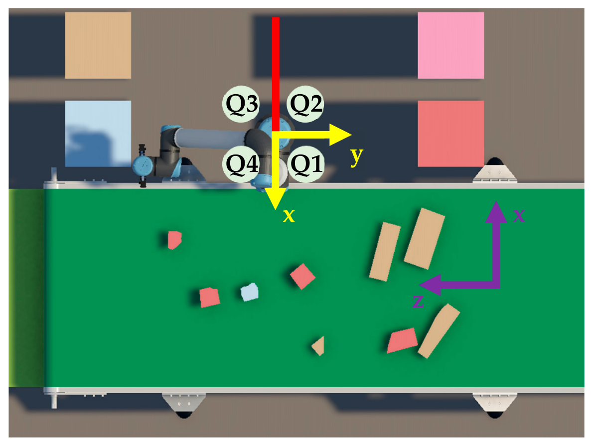
Table A1.
Quadrant-based goal redirection used by the safe target routine.
After any required redirection, let E and G denote the planar (xy plane) end effector and current goal positions relative to the robot base. The minimum distance between the base centre and the line segment joining E and G is calculated as
where clip(∙, 0, 1) constrains the projection to the finite line segment.
Let L denote the Cartesian look-ahead distance and D the detour step. If the remaining distance to the current goal is less than or equal to L, the goal itself is returned. Otherwise, when dseg ≥ rk, the direct path does not intersect the keep-out region, and the intermediate target is selected as distance L towards the goal:
where denotes either the original Cartesian goal or the redirected goal obtained from Table A1.
When dseg < rk, the same look-ahead point ptmp is first evaluated. If its planar distance from the base is already greater than or equal to rk, it is accepted directly. Otherwise, it is redirected towards a point immediately outside the keep-out boundary. Defining
the boundary point is located at planar coordinates , where is a small positive boundary offset. The intermediate target is then advanced by the detour distance D from the current end effector position towards this boundary point. As a final numerical safeguard, any resulting target lying inside rb is projected radially onto the boundary. Therefore, this procedure produces either the original goal, a normal look-ahead target, or a detour target outside the protected base region while preserving the vertical coordinate of the current goal. The values of Rk, mk, L, D, and used in the experiments are reported in Appendix A.7.
Appendix A.2. Feedforward Activation and Cartesian Velocity Saturation
The FF contribution in Equation (4) is activated according to the distance between the current end effector position and the actual Cartesian goal,
The activation factor is defined as
where ds is the distance at which FF compensation begins to activate and df is the distance at which the full FF contribution is applied. The cubic interpolation 3s2 − 2s3 provides a smooth transition between zero and full FF compensation, avoiding an abrupt change in the commanded velocity as the end effector approaches the target.
After either the FB or FF+FB raw translational command is calculated, its magnitude is constrained by the maximum Cartesian velocity vmax. Let vraw denote the corresponding raw command from Equation (3) or Equation (4). The velocity supplied to the Cartesian twist is
This saturation preserves the direction of the requested translational motion while limiting its magnitude to the configured Cartesian velocity bound. The values of ds, df, and vmax used in the experiments are reported in Appendix A.7.
Appendix A.3. Desired Tool Orientation
The desired tool orientation was constructed from the target orientation angle , which represents the yaw of the target long axis in the robot base xy plane. The tool z axis was directed vertically downward towards the conveyor, while the tool x axis was aligned perpendicular to the target long axis. The desired tool frame was therefore defined by
where xd, yd, and zd are the desired unit axes of the tool expressed in the robot base frame. The corresponding desired rotation matrix is formed using these vectors as its columns:
Let Re denote the current end effector rotation matrix expressed in the robot base frame. The commanded angular velocity is obtained from the skew symmetric component of the relative orientation between the desired and current tool frames as
where kr is the rotational FB gain and the vee(∙) operator is defined as
The value of kr used in the experiments is reported in Appendix A.7.
Appendix A.4. Null Space Posture Objective
The posture term in Equation (6) was projected using a damped task null space formulation to reduce its influence on the primary Cartesian tracking objective. The damped pseudoinverse of the Jacobian and the corresponding null space projector are defined as
where is the pseudoinverse damping coefficient and I is the identity matrix.
For the six-axis UR10e controlling a six-dimensional Cartesian twist, the Jacobian generally has no non-trivial exact null space at nonsingular configurations. Furthermore, the damped projector does not guarantee complete decoupling between posture restoration and Cartesian tracking. Therefore, the posture term acts as a soft regularisation objective that may influence the primary tracking task. Its influence is examined through an additional ablation experiment in Section 4.1.
The reference posture qref was initialised from the robot configuration when the controller was first activated and remained fixed during operation. The posture restoration velocity was calculated as
where ∆t is the control interval, sp is the posture velocity scaling factor, and is the effective velocity limit of joint i. The clip(∙) operation constrains each posture velocity component to the corresponding scaled joint velocity bound. The values of , sp, and the joint velocity limits are provided in Appendix A.7.
Appendix A.5. QP Safety Constraints
The generic QP constraint in Equation (7) combines vertical safety, self-collision avoidance, and joint position and velocity limits. Constraints that impose only a minimum allowable motion are represented by a finite lower bound and an unbounded upper bound, while the joint constraints use finite lower and upper bounds. The resulting constraint rows are assembled into A(q), l(q), and u(q).
Appendix A.5.1. End Effector Vertical Constraint
To prevent the end effector from moving below the minimum allowable height zplane, its vertical velocity is constrained by
where Je,z is the row of the end effector linear Jacobian corresponding to motion in the vertical direction, ze is the current end effector height, and is the corresponding safety gain. As the end effector approaches zplane, the allowable downward velocity is progressively reduced.
Appendix A.5.2. Forearm Vertical Constraint
The forearm constraint switches between relative clearance from the end effector and an absolute minimum height according to the current end effector height:
where Jf,z is the vertical component of the forearm point Jacobian, zf is the current forearm height, zswitch is the end effector height at which the constraint formulation changes, zf,min is the minimum allowable forearm height, and is the forearm safety gain. When the end effector is below zswitch, the first condition regulates the vertical separation between the forearm and end effector. Otherwise, the second condition maintains the forearm above its specified minimum height.
Appendix A.5.3. Self-Collision Constraints
Self-collision avoidance is formulated using the closest points between potentially colliding robot links. For candidate link pair i, let p1,i and p2,i denote the closest points on the two links, with separation distance di. The corresponding separation direction and constraint Jacobian are
where and are the linear velocity Jacobians evaluated at the corresponding closest points. The resulting constraint is
where dsafe is the required minimum link separation, regulates the approach towards the safe distance, and kpush specifies the corrective separation rate when the distance falls below dsafe.
Link distances are obtained through MoveIt. Adjacent and identical link pairs are excluded from consideration, candidate pairs are ordered by increasing separation distance, and only the closest Nc constraints are included in the QP at each control iteration. The corresponding parameter values are reported in Appendix A.7.
Appendix A.5.4. Joint Position and Velocity Constraints
Joint position and velocity restrictions are combined into a single allowable velocity interval for each joint. For joint i, the lower and upper velocity bounds are
with
where qi,min and qi,max are the position limits of joint i, mq is the joint limit margin, ∆t is the control interval, and is the effective velocity limit of the joint. This formulation ensures that the commanded motion respects both the joint position margin and the velocity limit within the next control interval. If the calculated lower bound exceeds the upper bound, the implementation sets the admissible velocity for that joint to zero. The numerical values of the safety gains, distance thresholds, joint limit margin, and related controller parameters are provided in Appendix A.7.
Appendix A.6. Solver and Emergency Collision Response
The QP was solved using OSQP at each control iteration. The solver was initialised using fixed Hessian and constraint sparsity patterns, while the numerical values of the objective and constraint matrices were updated according to the current robot state. Warm starting was enabled so that the solution from the preceding control iteration could be used to initialise the subsequent QP solve, reducing the computational overhead of repeated optimisation.
After the QP solution was obtained, an additional collision check was performed using the MoveIt collision model. If an actual self-collision was detected, the computed joint velocity command was replaced by a reduced command in the opposite direction,
where is the joint velocity obtained from the QP. This response acts as a fallback brake and reversal mechanism by attenuating and reversing the QP velocity command when an actual self-collision is detected.
Appendix A.7. Controller Parameters
Table A2.
Controller, safety, and implementation parameters used in the velocity control formulation.
Appendix B. Pick-and-Place Executor Configuration
Table A3.
Pick-and-place executor parameters used in the reported experiments.
References
- Dodampegama, S.; Hou, L.; Asadi, E.; Zhang, G.; Setunge, S. A YOLOv8x-Seg-Based Adversarial Domain Adaptation Approach for Construction and Demolition Waste Instance Segmentation. Int. J. Constr. Manag. 2026, 1–23. [Google Scholar] [CrossRef] [Scilit]
- Zhang, J.; Ma, M.; Zhang, G.; Dodampegama, S.; Li, C.-Q. Modelling System Evolving in Circular Economy Transitions: A Trajectory-Based Analysis of Carbon Saving. Int. J. Constr. Manag. 2025, 26, 2605–2626. [Google Scholar] [CrossRef] [Scilit]
- Dodampegama, S.; Hou, L.; Asadi, E.; Zhang, G.; Setunge, S. Revolutionizing Construction and Demolition Waste Sorting: Insights from Artificial Intelligence and Robotic Applications. Resour. Conserv. Recycl. 2024, 202, 107375. [Google Scholar] [CrossRef] [Scilit]
- Dodampegama, S.; Hou, L.; Asadi, E.; Reza-E-Rabbi, S.; Setunge, S.; Zhang, G. Digital and Intelligent Technologies for Construction and Demolition Waste Sorting: A Systematic Mapping Review of Research Maturity, Circularity Outcomes, and Industry Gaps. Sustainability 2026, 18, 10327. [Google Scholar] [CrossRef] [Scilit]
- Wang, Z.; Li, H.; Yang, X. Vision-Based Robotic System for on-Site Construction and Demolition Waste Sorting and Recycling. J. Build. Eng. 2020, 32, 101769. [Google Scholar] [CrossRef] [Scilit]
- Chen, X.; Huang, H.; Liu, Y.; Li, J.; Liu, M. Robot for Automatic Waste Sorting on Construction Sites. Autom. Constr. 2022, 141, 104387. [Google Scholar] [CrossRef] [Scilit]
- Prasad, V.; Arashpour, M. Enhancing Sorting Efficiency in Cluttered Construction and Demolition Waste Streams via Boundary-Guided Grasp Detection. Waste Manag. 2025, 207, 115123. [Google Scholar] [CrossRef] [Scilit] [PubMed]
- González Huarte, J.; Ibarguren, A. Visual Servoing Architecture of Mobile Manipulators for Precise Industrial Operations on Moving Objects. Robotics 2024, 13, 71. [Google Scholar] [CrossRef] [Scilit]
- Chen, X.; Liu, P.; Ying, R.; Wen, F. Autonomous 6-DOF Manipulator Operation for Moving Target by a Capture and Placement Control System. Sensors 2022, 22, 4836. [Google Scholar] [CrossRef] [Scilit] [PubMed]
- Wang, R.; Liang, C.; Pan, D.; Zhang, X.; Xin, P.; Du, X. Research on a Visual Servo Method of a Manipulator Based on Velocity Feedforward. Space Sci. Technol. 2021, 2021, 9763179. [Google Scholar] [CrossRef] [Scilit]
- Deng, Q.; Li, Z.; Huang, Q.; Yang, Q.; Bai, J. RGB-D Multimodal Fusion Perception-to-Action System for Automated Detection and Robotic Sorting of Construction and Demolition Waste. Autom. Constr. 2026, 192, 107268. [Google Scholar] [CrossRef] [Scilit]
- Kokkalis, K.; Konstantinidis, F.K.; Koskinopoulou, M.; Tsimiklis, G.; Amditis, A.; Frangos, P. RaapWaste: Robot- and Application-Agnostic Planning for Efficient Construction and Demolition Waste Sorting. Sustainability 2025, 17, 7293. [Google Scholar] [CrossRef] [Scilit]
- Dodampegama, S.; Singh, A.; Hou, L.; Asadi, E.; Zhang, K.; Setunge, S. A Digital Twin Simulation Framework for Conveyor-Based Construction Waste Sorting Using RGB-Derived Mesh Assets. In Proceedings of the International Symposium on Automation and Robotics in Construction; International Association for Automation and Robotics in Construction (IAARC): Edinburgh, UK, 2026; pp. 2401–2409. [Google Scholar] [CrossRef] [Scilit] [PubMed]
- Gao, Y.; Wang, J.; Xu, X. Machine Learning in Construction and Demolition Waste Management: Progress, Challenges, and Future Directions. Autom. Constr. 2024, 162, 105380. [Google Scholar] [CrossRef] [Scilit]
- Lin, K.; Zhou, T.; Gao, X.; Li, Z.; Duan, H.; Wu, H.; Lu, G.; Zhao, Y. Deep Convolutional Neural Networks for Construction and Demolition Waste Classification: VGGNet Structures, Cyclical Learning Rate, and Knowledge Transfer. J. Environ. Manag. 2022, 318, 115501. [Google Scholar] [CrossRef] [Scilit] [PubMed]
- Lu, W.; Chen, J.; Xue, F. Using Computer Vision to Recognize Composition of Construction Waste Mixtures: A Semantic Segmentation Approach. Resour. Conserv. Recycl. 2022, 178, 106022. [Google Scholar] [CrossRef] [Scilit]
- Demetriou, D.; Mavromatidis, P.; Robert, P.M.; Papadopoulos, H.; Petrou, M.F.; Nicolaides, D. Real-Time Construction Demolition Waste Detection Using State-of-the-Art Deep Learning Methods; Single-Stage vs Two-Stage Detectors. Waste Manag. 2023, 167, 194–203. [Google Scholar] [CrossRef] [Scilit] [PubMed]
- Demetriou, D.; Mavromatidis, P.; Petrou, M.F.; Nicolaides, D. CODD: A Benchmark Dataset for the Automated Sorting of Construction and Demolition Waste. Waste Manag. 2024, 178, 35–45. [Google Scholar] [CrossRef] [Scilit] [PubMed]
- Sirimewan, D.; Harandi, M.; Peiris, H.; Arashpour, M. Semi-Supervised Segmentation for Construction and Demolition Waste Recognition in-the-Wild: Adversarial Dual-View Networks. Resour. Conserv. Recycl. 2024, 202, 107399. [Google Scholar] [CrossRef] [Scilit]
- Sirimewan, D.; Kunananthaseelan, N.; Raman, S.; Garcia, R.; Arashpour, M. Optimizing Waste Handling with Interactive AI: Prompt-Guided Segmentation of Construction and Demolition Waste Using Computer Vision. Waste Manag. 2024, 190, 149–160. [Google Scholar] [CrossRef] [Scilit] [PubMed]
- Prasad, V.; Arashpour, M. Optimally Leveraging Depth Features to Enhance Segmentation of Recyclables from Cluttered Construction and Demolition Waste Streams. J. Environ. Manag. 2024, 354, 120313. [Google Scholar] [CrossRef] [Scilit] [PubMed]
- Prasad, V.; Arashpour, M. Real-Time Instance Segmentation of Recyclables from Highly Cluttered Construction and Demolition Waste Streams. J. Environ. Manag. 2024, 372, 123365. [Google Scholar] [CrossRef] [Scilit] [PubMed]
- Prasad, V.; Arashpour, M. ShARP-WasteSeg: A Shape-Aware Approach to Real-Time Segmentation of Recyclables from Cluttered Construction and Demolition Waste. Waste Manag. 2025, 195, 231–239. [Google Scholar] [CrossRef] [Scilit] [PubMed]
- Sirimewan, D.; Dayarathna, S.; Raman, S.; Bai, Y.; Arashpour, M. A Benchmark Dataset for Class-Wise Segmentation of Construction and Demolition Waste in Cluttered Environments. Sci. Data 2025, 12, 885. [Google Scholar] [CrossRef] [Scilit] [PubMed]
- Lin, Y.-H.; Mao, W.-L.; Fathurrahman, H.I.K. Development of Intelligent Municipal Solid Waste Sorter for Recyclables. Waste Manag. 2024, 174, 597–604. [Google Scholar] [CrossRef] [Scilit] [PubMed]
- Cheng, T.; Kojima, D.; Hu, H.; Onoda, H.; Pandyaswargo, A.H. Optimizing Waste Sorting for Sustainability: An AI-Powered Robotic Solution for Beverage Container Recycling. Sustainability 2024, 16, 10155. [Google Scholar] [CrossRef] [Scilit]
- Halvorsen, T.S.; Tyapin, I.; Jha, A. Autonomous Textile Sorting Facility and Digital Twin Utilizing an AI-Reinforced Collaborative Robot. Electronics 2025, 14, 2706. [Google Scholar] [CrossRef] [Scilit]
- Sinico, T.; Businaro, D.; Boschetti, G. Integrating Vision–Language–Action Models and RGB-D Sensing for Robotic Waste Sorting on KUKA LBR Iiwa. Robotics 2026, 15, 100. [Google Scholar] [CrossRef] [Scilit]
- Wang, F.; Ren, B.; Liu, Y.; Cui, B. Tracking Moving Target for 6 Degree-of-Freedom Robot Manipulator with Adaptive Visual Servoing Based on Deep Reinforcement Learning PID Controller. Rev. Sci. Instrum. 2022, 93, 045108. [Google Scholar] [CrossRef] [Scilit] [PubMed]
- Pi, J.; Zhang, W.; Zhang, S.; Pi, C.; Xie, C. Capturing the Dynamic Target by the Robot Manipulator in High-Dimensional Configuration Space Map. Int. J. Adv. Robot. Syst. 2020, 17, 1729881420939441. [Google Scholar] [CrossRef] [Scilit]
- Chen, Z.-H.; Xu, Z.-D.; Lu, H.-F.; Yang, J.-Z.; Yu, D.-Y.; Zhu, C.; Zhen, S.-C.; Zheng, H.-M. A New Robust Control Strategy for Axial Flux Permanent Magnet Motor Applied on Legged Lunar Robots. J. Vib. Control 2023, 29, 953–967. [Google Scholar] [CrossRef] [Scilit]
- Chen, Z.-H.; Xu, Z.-D.; Wang, R.-H.; Lu, H.-F.; Yu, D.-Y.; Yang, J.-Z.; Zhao, X.-L.; Hu, Z.-W.; Zhen, S.-C. Robust Control Algorithm Designed for Robotic Legs of Lunar-Based Equipment: Modeling and Experiment. Adv. Space Res. 2024, 74, 3945–3957. [Google Scholar] [CrossRef] [Scilit]
- Chen, Z.-H.; Xu, Z.-D.; Lu, H.-F.; Yu, D.-Y.; Yang, J.-Z.; Pan, B.; Zhao, X.-L.; Hu, Z.-W.; Zhen, S.-C. Novel Robust Control Strategy for the Mechanical Legs of Lunar-Based Equipment. J. Aerosp. Eng. 2023, 36, 04023061. [Google Scholar] [CrossRef] [Scilit]
- Chen, Z.-H.; Xu, Z.-D.; Lu, H.-F.; Yu, D.-Y.; Yang, J.-Z.; Pan, B.; Zhao, X.-L.; Hu, Z.-W. Novel Robust Control Method for Leg-Soil System of Lunar-Based Equipment. Int. J. Struct. Stab. Dyn. 2024, 24, 2450172. [Google Scholar] [CrossRef] [Scilit]
- Flores-Campos, J.A.; Torres-San-Miguel, C.R.; Paredes-Rojas, J.C.; Perrusquía, A. Prescribed Time Interception of Moving Objects’ Trajectories Using Robot Manipulators. Robotics 2024, 13, 145. [Google Scholar] [CrossRef] [Scilit]
- Righettini, P.; Strada, R.; Cortinovis, F. Neural Network Mapping of Industrial Robots’ Task Times for Real-Time Process Optimization. Robotics 2023, 12, 143. [Google Scholar] [CrossRef] [Scilit]
- Carlier, R.; Gillis, J.; De Clercq, P.; Borghesan, G.; Stockman, K.; De Kooning, J.D.M. Performance Gain of Collaborative Versus Sequential Motion in Modular Robotic Manipulators for Pick-and-Place Operations. Machines 2025, 13, 348. [Google Scholar] [CrossRef] [Scilit]
- Marauli, T.; Gratt, F.; Gattringer, H.; Müller, A. Nearly Time-Optimal Online Pick and Place Trajectory Computation Using Quadratic Programming. IFAC-PapersOnLine 2025, 59, 277–282. [Google Scholar] [CrossRef] [Scilit]
- Cao, Y.; Xu, X.; Zhang, Y. Vision-Based Reinforcement Learning for Robotic Grasping of Moving Objects on a Conveyor. Machines 2025, 13, 973. [Google Scholar] [CrossRef] [Scilit]
- Ladefoged, M.B.; Larsen, A.K.; Vasegaard, A.E.; Nielsen, P. The Value of Information in Automated Sorting: Leveraging Look-Ahead in Multi-Conveyor Systems with Articulated Robotics for Pick and Place. J. Ind. Prod. Eng. 2026, 1–18. [Google Scholar] [CrossRef] [Scilit]
- Steinert, G.; Troll, C.; Majschak, J.-P. Bilevel Trajectory Optimization for Vacuum-Based Pick-and-Place Operations: A Numerical Study. Robotics 2026, 15, 126. [Google Scholar] [CrossRef] [Scilit]
- Li, Y.; Zhang, Q.; Xu, H.; Lim, E.; Sun, J. Virtual Monitoring System for a Robotic Manufacturing Station in Intelligent Manufacturing Based on Unity 3D and ROS. Mater. Today Proc. 2022, 70, 24–30. [Google Scholar] [CrossRef] [Scilit]
- Singh, M.; Kapukotuwa, J.; Gouveia, E.L.S.; Fuenmayor, E.; Qiao, Y.; Murry, N.; Devine, D. Unity and ROS as a Digital and Communication Layer for Digital Twin Application: Case Study of Robotic Arm in a Smart Manufacturing Cell. Sensors 2024, 24, 5680. [Google Scholar] [CrossRef] [Scilit] [PubMed]
- Boschetti, G.; Sinico, T. Designing Digital Twins of Robots Using Simscape Multibody. Robotics 2024, 13, 62. [Google Scholar] [CrossRef] [Scilit]
- Singh, M.; Kapukotuwa, J.; Gouveia, E.L.S.; Fuenmayor, E.; Qiao, Y.; Murray, N.; Devine, D. Comparative Study of Digital Twin Developed in Unity and Gazebo. Electronics 2025, 14, 276. [Google Scholar] [CrossRef] [Scilit]
- Kawshan, D.; Peng, Q. Digital Twin Framework for Robot Path Planning and Real-Time Execution Using Unity-ROS Integration: Systems Architecture and Experimental Validation. Machines 2026, 14, 387. [Google Scholar] [CrossRef] [Scilit]
- Pantusin, F.J.; Ortiz, J.S.; Carvajal, C.P.; Andaluz, V.H.; Yar, L.G.; Roberti, F.; Gandolfo, D. Digital Twin Integration for Active Learning in Robotic Manipulator Control Within Engineering 4.0. Symmetry 2025, 17, 1638. [Google Scholar] [CrossRef] [Scilit]
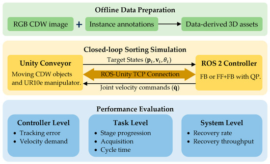
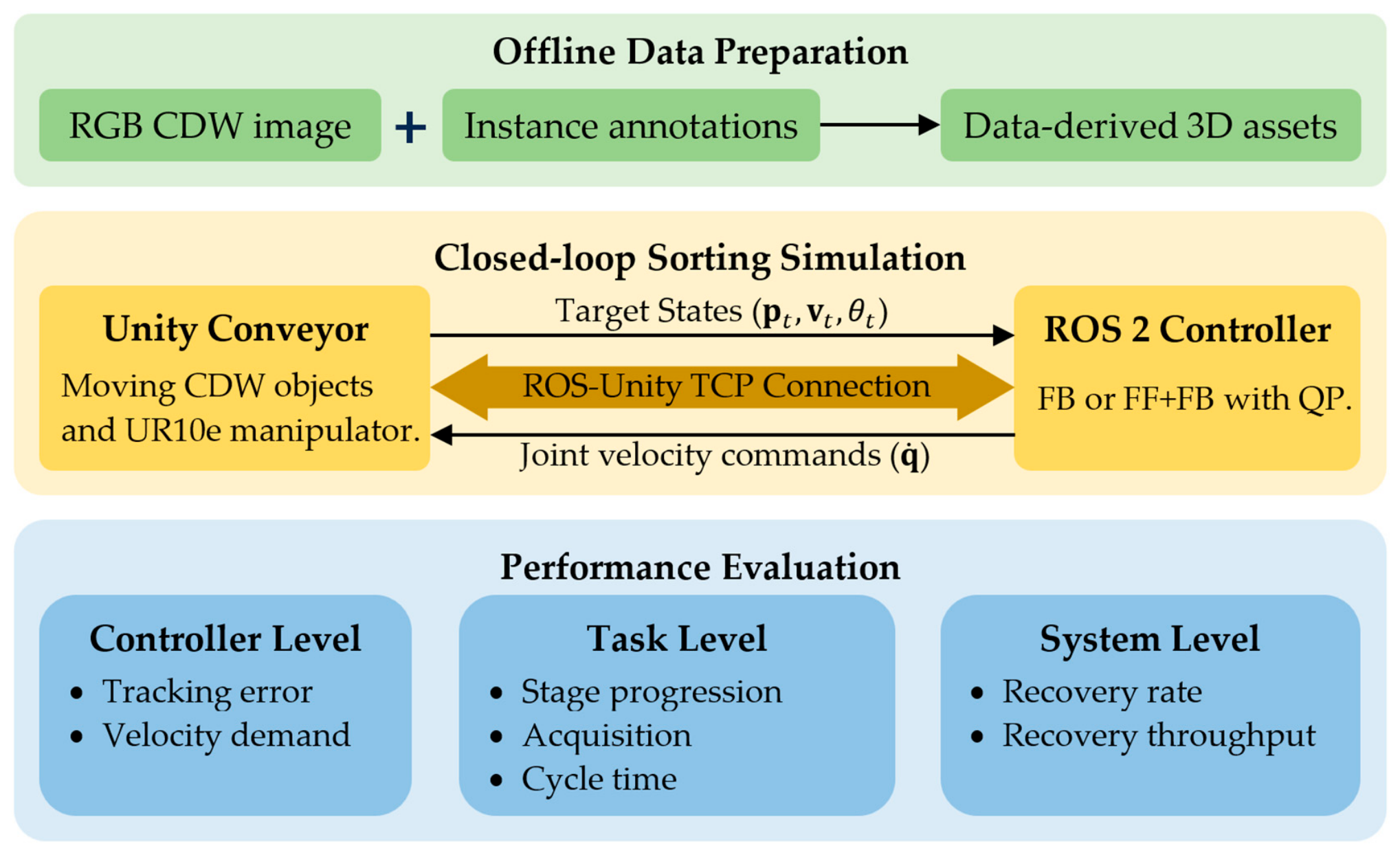
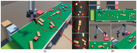
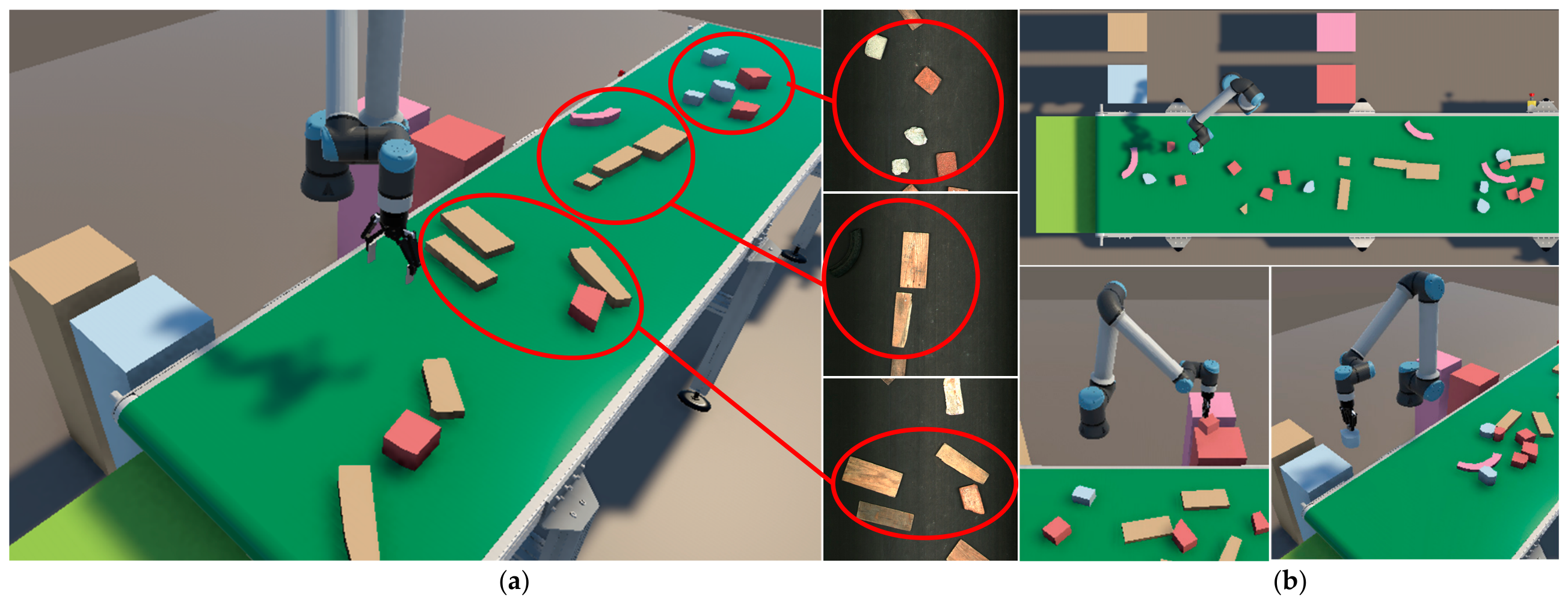
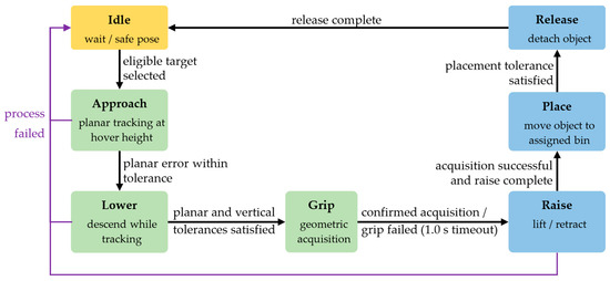
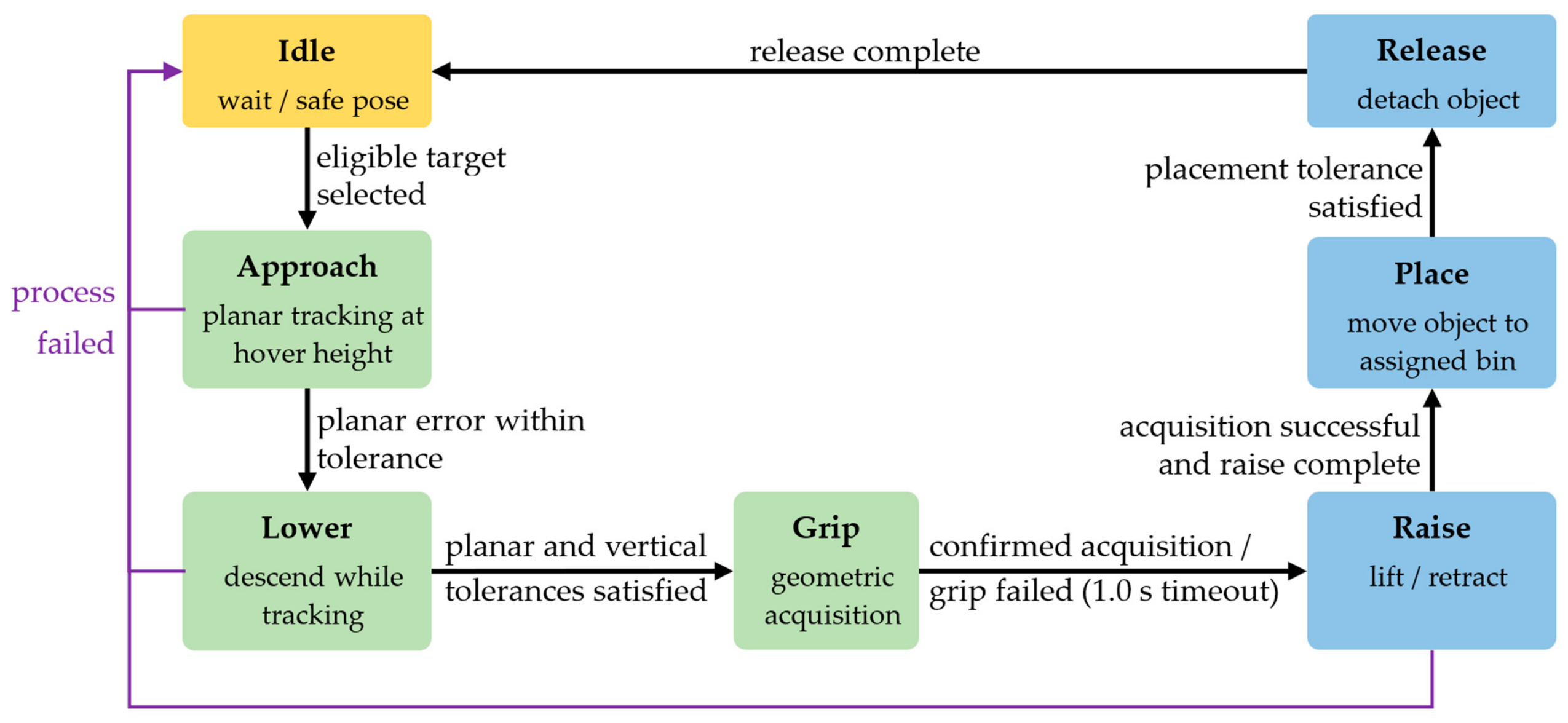
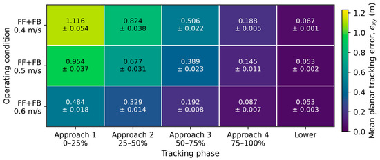
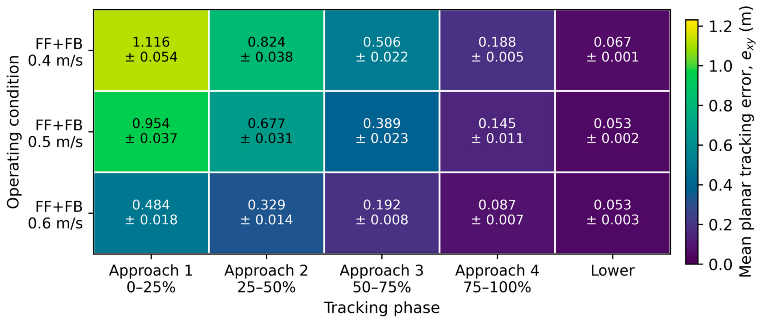
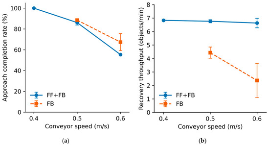
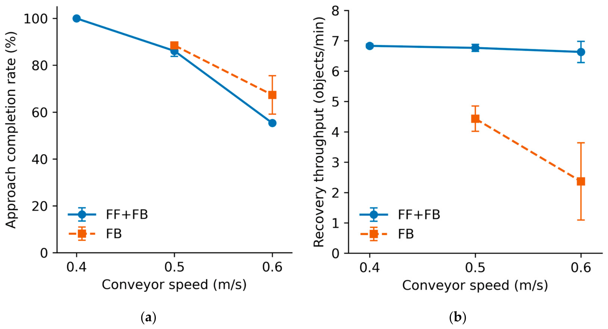

Disclaimer/Publisher’s Note: The statements, opinions and data contained in all publications are solely those of the individual author(s) and contributor(s) and not of MDPI and/or the editor(s). MDPI and/or the editor(s) disclaim responsibility for any injury to people or property resulting from any ideas, methods, instructions or products referred to in the content. |
© 2026 by the authors. Licensee MDPI, Basel, Switzerland. This article is an open access article distributed under the terms and conditions of the Creative Commons Attribution (CC BY) license.