“Square-Root” Klein–Gordon Equation: The Harmonic and Morse Potentials

Abstract

Quantum relativistic solutions of a “square-root” version of the Klein–Gordon equation, for a particle in a one-dimensional Morse potential, are presented using methods previously proposed and applied to a particle in a harmonic oscillator. The methods lead to both numerical and analytical solutions, with the latter allowing smooth variation of the system parameters from non-relativistic to ultra-relativistic limits. Analytical expressions for the energy levels and wavefunctions are obtained, as solutions to a Schrödinger-type equation, including relativistic effects through a state-dependent rescaled mass. The eigenstates of the Morse potential exhibit suitable and smooth behavior and approach the corresponding harmonic oscillator solutions as the depth of the Morse potential well increases, as expected. A comparison is also presented between the relativistic harmonic oscillator obtained with this method and the so-called “Klein–Gordon oscillator”.

1. Introduction

Potentials have wide applicability in atomic, molecular, and physical chemistry physics. Scientists in all of these disciplines routinely use the form of the potential to guide their classical and quantum intuition about how systems behave. But for the most part, this intuition is based on non-relativistic forms of the kinetic energy. How does this situation change in the relativistic context? Even more broadly, one may question the very form of the relativistic Hamiltonian itself—or, as our collaborator L. Grave de Peralta has put it, “Did Schrödinger have other options?”.

A natural test case for addressing such questions is, of course, the quintessential harmonic oscillator potential. Traditionally, the quantum problem of a particle in a harmonic potential enters the relativistic domain through the so-called Dirac [1] and Klein–Gordon oscillators [2]. The Dirac oscillator is defined by applying the non-minimal coupling $\widehat{\mathbf{p}}-im\omega \mathbf{r}$ to the free-particle Dirac equation. With this substitution, the large-component wave equation tends, in the non-relativistic limit, to a Schrödinger-like equation, with the Hamiltonian of a harmonic oscillator of frequency $\omega$ and a spin-orbit coupling of strength $-2\omega /\hslash$. This led the authors to name the model the “Dirac oscillator” (DO) [1]. The DO has attracted attention due to its capability of describing quark confinement [3] and its relevance for quantum optics after noticing its connection with the Jaynes–Cummings model [4]. Recent reports suggest experimental confirmation of the DO [5].

Following the same spirit, the Klein–Gordon oscillator (KGO) was proposed [2] for a spin-0 particle as the solution of the free-particle Klein–Gordon (KG) equation, modified with the non-minimal coupling prescription,

$${\widehat{p}}^2\to \left(\widehat{p}+im\omega x\right)\left(\widehat{p}-im\omega x\right)$$

(1)

where we are now considering the one-dimensional (1D) case (for the general case, see Ref. [2]).

Plugging Equation (1) into the free-particle KG equation leads to a Schrödinger-like equation for a particle of mass m in a harmonic potential of frequency $\omega$. The eigenenergies of this equation are non-linear functions of the corresponding Schrödinger values, which they approach (apart from an additive constant) in the non-relativistic limit. The KGO has attracted interest as a relativistic model in non-commutative spaces [6] and curved space-time [7]. However, it manifests some issues—highlighting the need for something better. Note that in Section 5 of this work, we explicitly compare the KGO results with those of the present methods applied to the harmonic oscillator.

Beyond the harmonic potential, another Schrödinger oscillator problem that has been considered in a relativistic context is that of a particle in a Morse potential (MP) [8]. In 1D, the MP can be written,

$${\widehat{V}}_{\mathrm{M}}\left(x\right)=D{(1-e^{-\alpha x})}^2$$

(2)

The above MP expression describes a bounded well region of depth D and width $(1/\alpha )$, centered around the origin $x=0$, which grows exponentially quickly for $x<0$ and approaches the dissociation energy $V_{\mathrm{M}}\left(x\right)\to D$ with exponential decay as $x\to \infty$. These are recognized qualitative features of the potential energy curve for a covalently bound diatomic molecule as a function of internuclear separation. In this sense, the MP has a reputation as one of the first models to accurately describe the vibrational energy levels of diatomic molecules [8]—including the finiteness of the bound spectrum and the anharmonic decrease in level spacing with increasing energy excitation.

On the other hand, the MP has also found other applications, as a model for surface-surface interactions [9] and to accurately describe spectroscopic data, when generalized to account for long-range molecular forces [10]. Of course, for these nuclear motion applications, relativistic effects are expected to be vanishingly small (an estimate is provided in Section 6). On the other hand, an interesting relativistic application of the MP was recently considered [11], involving a relativistic electron exhibiting Schottky anomalies—which are caused by the finiteness of the discrete spectrum and hence well described by an MP model.

The relativistic MP is defined in [11] by recasting the free-particle KG equation with the ansatz (1) in a transformed coordinate $\eta$ (with non-additive spatial displacement), generated by the coordinate-dependent momentum operator,

$${\widehat{p}}_{\alpha }=-i\hslash (1-\alpha \eta ){\displaystyle \frac{d}{d\eta }}.$$

(3)

This leads to a “deformed” KGO equation [11]. Then, upon applying the particular coordinate transformation,

$$\eta ={\displaystyle \frac{1-e^{-\alpha x}}{\alpha }},$$

(4)

one obtains a Schrödinger-like equation for a particle in an MP. The interested reader is directed to Ref. [11] for further details.

Although it is not clear whether this non-minimal coupling scheme serves to extend any arbitrary potential problem to the relativistic domain, it certainly avoids the pitfalls that are encountered when one instead includes the potential energy in the time-like component of the four-momentum potential operator in the KG equation. In this case, the equation becomes

$$(m^2+{\widehat{p}}^2)\psi ={(E-\widehat{V})}^2\psi .$$

(5)

Note that in Equation (5) above—and throughout this paper—units are adopted for which $c=1$. In effect, this leaves m as the relativistic parameter, with ultra-relativistic and non-relativistic limits corresponding to $m\to 0$ and $m\to \infty$, respectively.

Equation (5) can be written as a non-linear Schrödinger-like equation for a particle with effective energy $(E^2-m^2)/2m$, moving in an effective potential,

$${\widehat{V}}_{\mathrm{eff}}={\displaystyle \frac{2E\widehat{V}-{\widehat{V}}^2}{2m}}.$$

(6)

Thus, any bound oscillator solutions are in fact eigenstates of different energy-dependent Hamiltonians, that are not generally orthogonal. Even more problematic, however, is the fact that if $\widehat{V}\to \pm \infty$ in either asymptotic limit, then the $-{\widehat{V}}^2$ term creates a “hole” that causes ${\widehat{V}}_{\mathrm{eff}}\to -\infty$. The resulting eigensolutions are thus non-square integrable solutions and are in fact shape resonances. More generally, it is not possible to obtain ${\widehat{V}}_{\mathrm{eff}}\to +\infty$ following this approach.

In recent work by the authors, the quantum relativistic problem of a particle in a one-dimensional potential $\widehat{V}\left(x\right)$ [12] has been addressed by taking another, less orthodox path [13,14,15]. In this approach, one solves a so-called “square-root” version of the Klein–Gordon equation (essentially what we have called the “PGP Equation” in previous work [13]),

$$\left[\sqrt{m^2+{\widehat{p}}^2}-m+\widehat{V}\left(x\right)\right]\psi \left(x\right)=E\psi \left(x\right),$$

(7)

where the relativistic rest energy has now been subtracted from both sides in order to result in an energy E that can be directly compared with the usual non-relativistic values. The chief obstacle in Equation (7) is the square-root operator (SRO) $\sqrt{m^2+{\widehat{p}}^2}$, and attempts to bypass this have led to the well-known Klein–Gordon [16,17] and Dirac [18] formulations of relativistic quantum mechanics.

The “chief complaint” about the SRO is that it is evidently non-local in x. Nevertheless, from a strictly mathematical perspective, this does not prevent one from obtaining—for a given bound-well oscillator potential $\widehat{V}\left(x\right)$—square-integrable, orthogonal, physically meaningful, and otherwise well-behaved solutions of Equation (7). This was demonstrated in [14] for the problem of a particle in a harmonic potential.

Several methods have been proposed for solving Equation (7), both exact and approximate [13,14]. First, the SRO can be replaced with an exact continued fraction representation that automatically singles out the correct positive-energy root. The continued fraction form, moreover, gives rise to a mean-field-type form based on expectation values, thus allowing one to write Equation (7) (approximately) as a non-linear (in $\psi$) Schrödinger-type equation. The solutions of the latter approximation can then be obtained using common iterative mean-field-type approaches [13]. The particular version of this approach used here has been called the “GPPP method” [13,14].

Applied to the harmonic oscillator problem, the above GPPP mean-field approximation turned out to be very straightforward—leading to analytical solutions that demonstrate physically correct behaviors in the ultra-relativistic limit [14] (unlike, e.g., the KGO; see Section 5). Second, an algorithm for obtaining numerically exact solutions of Equation (7) was presented [14], taking advantage of the fact that the SRO has diagonal positive-definite analytical matrix representation in a particle-in-box basis set. The numerical solutions, moreover, were found to be bound, orthogonal, etc., and otherwise behaved exactly as expected. Third, it was shown that analytical expressions for the energy values of a particle in a harmonic oscillator can be readily obtained, from the action-quantized condition, as prescribed within the standard Wentzel–Kramers–Brillouin (WKB) semiclassical theory [14]. It is worth noting that all the methods mentioned above show good agreement with each other (but not with the KGO) for variations of system parameters ranging from non-relativistic to ultra-relativistic limits [14].

In this paper, the same techniques will be applied to the problem of a particle in a Morse potential. In particular, this work mainly addresses a comparison between numerically exact solutions of the square-root Klein–Gordon equation and the GPPP approximation. Although the application of the methods appears to be less straightforward in this case, analytical expressions are obtained for the energy levels of the Morse potential that correctly approach the harmonic oscillator solutions as the depth of the MP well increases. An important result concerns the derivation of analytical expressions for the number of MP energy levels, as a function of the well depth and width, to encompass variation of system parameters ranging from non-relativistic to ultra-relativistic limits.

The remainder of this paper is organized as follows. The next section briefly summarizes the GPPP method and presents the main results already published [14] for the harmonic oscillator system. Section 3 is devoted to the application of the GPPP method to the approximate solution of Equation (7), for the Morse potential ${\widehat{V}}_M\left(x\right)$, while the same problem is addressed, in Section 4, using the approximate WKB and exact numerical methods. Section 5 presents a comparison between the approximate GPPP solution of Equation (7) and the corresponding KGO energy eigenvalues. It should be noted that this comparison is limited to the harmonic oscillator system; a detailed study including the MP will be addressed in future work. Finally, some concluding remarks are presented in Section 6.

2. The GPPP Method

2.1. Introduction to the Method

The operation of the particular mean-field approximation alluded to above, which is called the “Grave de Peralta Poveda Poirier (GPPP) approach” [13,14] will be described in this section. We start by writing Equation (7) in the following equivalent form (aka the “Poirier-Grave de Peralta (PGP) Equation”),

$$\left[{\displaystyle \frac{{\widehat{p}}^2}{(1+\widehat{\gamma })m}}+\widehat{V}\right]\psi =E\psi ,$$

(8)

which includes the SRO,

$$\widehat{\gamma }=\sqrt{1+{\displaystyle \frac{{\widehat{p}}^2}{m^2}}}.$$

(9)

Here, the momentum operator has its usual interpretation, i.e., $\widehat{p}=-i\hslash d/dx$. It is worth noting that Equation (8) is the same as Equation (7), obtained by conveniently rearranging the square root (see [13,14] for further details).

In order to avoid the cumbersome SRO $\widehat{\gamma }$, it is replaced with its expectation value $⟨\psi \mid \widehat{\gamma }\mid \psi ⟩$, for each of the eigenstates $\psi$ of Equation (8). Of course, we do not actually know the exact eigenstates. So, in practice, we work with the approximate solution eigenstates ${\psi }_{\mathrm{GPPP}}$, leading to [13]

$$\left({\displaystyle \frac{{\widehat{p}}^2}{2\mu }}+\widehat{V}\right){\psi }_{\mathrm{GPPP}}=E_{\mathrm{GPPP}}{\psi }_{\mathrm{GPPP}},$$

(10)

where

$$\mu ={\displaystyle \frac{1+⟨{\psi }_{\mathrm{GPPP}}\mid \widehat{\gamma }\mid {\psi }_{\mathrm{GPPP}}⟩}{2}}m.$$

(11)

Equation (10) is thus the usual non-relativistic Schrödinger equation, but with a rescaled state-dependent effective mass $\mu$, that accounts for the relativistic kinetic energy of a particular eigenstate in a mean-field sense.

Note that Equation (10) is a non-linear (in ${\psi }_{\mathrm{GPPP}}$) Schrödinger equation, subject to a self-consistency condition, whose solution requires taking the SRO mean field average. A simplification can be obtained for the price of a further approximation,

$$⟨{\psi }_{\mathrm{GPPP}}\mid \widehat{\gamma }\mid {\psi }_{\mathrm{GPPP}}⟩\approx 1+{\displaystyle \frac{E_{\mathrm{GPPP}}-⟨{\psi }_{\mathrm{GPPP}}\mid \widehat{V}\mid {\psi }_{\mathrm{GPPP}}⟩}{m}},$$

(12)

which follows from Equation (7) [14]. Replacing Equation (12) into (11) leads to a rescaled mass

$$\mu \approx m+{\displaystyle \frac{E_{\mathrm{GPPP}}-⟨{\psi }_{\mathrm{GPPP}}\mid \widehat{V}\mid {\psi }_{\mathrm{GPPP}}⟩}{2}},$$

(13)

involving expectation values not of the SRO (as in Equation (11)) but of the much simpler potential operator, $\widehat{V}$.

The significance here is due to the fact that Equation (10) implies that all ${\psi }_{\mathrm{GPPP}}$ solutions are in fact just mass-rescaled versions of the non-relativistic solutions—for which analytical formulas for ${\widehat{p}}^2$ and $\widehat{V}$ are often known. This motivated a new approximation, for which both Equations (12) and (13) are assumed to be exactly true. What in effect this enables one to do is to solve the self-consistency problem directly for the parameter $\mu$ itself, without having to explicitly compute expectation values or perform iterative cycles.

We call this final approach the “self-consistent-GPPP (SC-GPPP) method” [14]. It is easy to show that the energy value associated with a normalized SC-GPPP wavefunction can be written as

$$E_{\mathrm{SC}–\mathrm{GPPP}}=\sqrt{m^2+⟨{\psi }_{\mathrm{SC}–\mathrm{GPPP}}\mid {\widehat{p}}^2\mid {\psi }_{\mathrm{SC}–\mathrm{GPPP}}⟩}-m+⟨{\psi }_{\mathrm{SC}–\mathrm{GPPP}}\mid \widehat{V}\mid {\psi }_{\mathrm{SC}–\mathrm{GPPP}}⟩,$$

(14)

where, again, ${\psi }_{\mathrm{SC}–\mathrm{GPPP}}$ is a mass-rescaled non-relativistic solution. Note that Equation (14) manifests the correct relativistic energy–momentum relation through expectation values. In what follows, unless otherwise stated, the symbols E and $\psi$ refer to the SC-GPPP energy and wavefunctions, respectively.

From Equation (10), with $\mu$ given by Equation (13), the SC-GPPP energy values can be straightforwardly obtained if the corresponding non-relativistic energy value (denoted $\mathcal{E}$) is known in closed form as a function of the particle mass m. Thus, provided that the function $\mathcal{E}=f\left(m\right)$ is known, the corresponding SC-GPPP energy value E will be the fixed points of the function $f\left[\mu \right(E\left)\right]$, or the solutions of the equation,

$$E=f\left(m+{\displaystyle \frac{E-⟨\widehat{V}⟩}{2}}\right).$$

(15)

Once E is determined as above, its associated SC-GPPP wavefunction can then be obtained by replacing the mass m in the familiar Schrödinger wavefunction with the state-dependent rescaled mass $\mu (E,\psi )$.

2.2. SC-GPPP Solutions for the Harmonic Oscillator

In this section, the method is briefly illustrated via application to a harmonic oscillator (HO) potential with force constant k, defined as the product of the square of the oscillator frequency and the mass of the particle. For a detailed discussion, see Ref. [14]. Here, the non-relativistic nth energy eigenvalue is well known to be

$${\mathcal{E}}_n=\left(n+{\displaystyle \frac{1}{2}}\right)\hslash \sqrt{{\displaystyle \frac{k}{m}}}.$$

(16)

The corresponding relativistic SC-GPPP energy is

$$E_n=\left(n+{\displaystyle \frac{1}{2}}\right)\hslash \sqrt{{\displaystyle \frac{k}{{\mu }_n}}},$$

(17)

with ${\mu }_n$ itself a function of the level energy $E_n$, through Equation (13).

In this case, the term $⟨\psi \mid \widehat{V}\mid \psi ⟩$ is very easy to evaluate. Since the corresponding result for the non-relativistic Schrödinger solutions ${\varphi }_n$ are well known to be $⟨{\varphi }_n\mid \widehat{V}\mid {\varphi }_n⟩={\mathcal{E}}_n/2$, this implies that

$$⟨{\psi }_n\mid \widehat{V}\mid {\psi }_n⟩={\displaystyle \frac{E_n}{2}},$$

(18)

which leads to the following equation for the SC-GPPP energy levels of the relativistic HO [14]:

$$E_n={\displaystyle \frac{{\mathcal{E}}_n}{\sqrt{1+{\displaystyle \frac{E_n}{4m}}}}}.$$

(19)

Note that the solutions to the equation above correspond to the fixed points of the function

$$f_n\left(E\right)={\displaystyle \frac{{\mathcal{E}}_n}{\sqrt{1+{\displaystyle \frac{E}{4m}}}}}.$$

(20)

The n-th solution of Equation (19) is well defined for every finite value of the parameter m, including in the ultra-relativistic limit, $m\to 0$. One way to obtain the solution is to start with the non-relativistic results as the zeroth-order guess—i.e., $E^{\left(0\right)}={\mathcal{E}}_n$—and then iterate via $E^{\left(s\right)}=f_n\left[E^{(s-1)}\right]$ until sufficient numerical convergence is achieved. Note that the relativistic increase in effective mass ensures monotonic convergence towards the fixed point $E_n<{\mathcal{E}}_n$. Also note that this fixed point is one of the real roots of the cubic equation,

$$E_n^3+4m{E}_n^2-4m{\mathcal{E}}_n^2=0,$$

(21)

so that, in this case at least, analytic solutions may be easily obtained.

In the non-relativistic limit $m\to \infty$, Equation (21) reduces to

$$E_n={\mathcal{E}}_n-{\displaystyle \frac{{\mathcal{E}}_n^2}{8m}}.$$

(22)

In this manner, the relativistic SC-GPPP energy levels approach the non-relativistic ones as expected, with a small second-order correction. On the other hand, in the ultra-relativistic limit $m\to 0$, mass-independent solutions are obtained [14]:

$$E_n={\left[2\left(n+{\displaystyle \frac{1}{2}}\right)\hslash \right]}^{2/3}{k}^{1/3}.$$

(23)

This behavior is physically correct, but, in any event, the solutions provide a reasonable and unified description throughout the entire range of possible mass values.

The equation above indicates that, in the ultra-relativistic limit, the level energy shows a sub-linear $\sim n^{2/3}$ power law scaling in n, corresponding to a level spacing which decreases in an inverse cubic root dependence with n [14]. The loss of the evenly spaced spectra, when moving to the relativistic domain, has effectively also been observed for a classical relativistic particle moving in a quadratic potential [19]. In this case, the period of oscillation increases with energy due to the time dilation along the world line [19].

3. The Morse Oscillator

3.1. Schrödinger Solution

Considering that GPPP is a Schrödinger-like approach to relativistic quantum mechanics, it is convenient to review the main result of the non-relativistic MP system. The MP was originally proposed [8] to accurately describe the low-lying vibrational energy levels of a diatomic molecule—up to second-order corrections in the excitation level index n [8]. Remarkably, the non-relativistic problem proved to be exactly solvable [8,20] within the wave-mechanical molecular description [21].

The shape of the MP (see Figure 4) implies both a set of discrete bound states for energies $E<D$ and also a continuum of scattering states above the dissociation energy $E=D$. In this work, we are interested only in the former, computing both SC-GPPP and numerically exact solutions. Note that the number of MP bound states is always finite but increases with the mass m, as well as the well depth D and width $(1/\alpha )$.

For the non-relativistic MP, the n-th energy level is found to be given by [8,20]

$${\mathcal{E}}_{\mathrm{M},n}=\left(n+{\displaystyle \frac{1}{2}}\right)\hslash \alpha \sqrt{{\displaystyle \frac{2D}{m}}}-{\left(n+{\displaystyle \frac{1}{2}}\right)}^2{\displaystyle \frac{{\hslash }^2{\alpha }^2}{2m}},$$

(24)

and analytical forms for the corresponding eigenstate wavefunctions are also known in terms of Laguerre polynomials [20]. Using Equation (16), Equation (24) can be written in the following compelling form:

$${\mathcal{E}}_{\mathrm{M},n}={\mathcal{E}}_{\mathrm{H},n}-{\displaystyle \frac{{\mathcal{E}}_{\mathrm{H},n}^2}{4D}}.$$

(25)

Here, ${\mathcal{E}}_{\mathrm{H},n}$ represents the n-th energy level of a harmonic oscillator with force constant $k=2D{\alpha }^2$.

Equation (25) suggests an interesting connection between the Morse and harmonic potentials. For a given MP with parameters D and $\alpha$, a unique HO can be associated with force constant $k=2D{\alpha }^2$ such that the allowed energy levels of the former can be obtained from the corresponding energy levels of the latter. This allows us to replace the MP parameter $\alpha$ with the associated harmonic potential parameter k, which we find convenient for the expressions that follow.

Note that Equation (25) is second order in ${\mathcal{E}}_{\mathrm{H},n}$, indicating that for each value ${\mathcal{E}}_{\mathrm{M},n}$ there are two possible values of ${\mathcal{E}}_{\mathrm{H},n}$. For example, the energy ${\mathcal{E}}_{\mathrm{M},0}=0.4875$, corresponding to the ground state of the MP with $\hslash =k=m=1$ and $D=5$, can be obtained, using Equation (25), from the energy levels ${\mathcal{E}}_{\mathrm{H},0}=0.5$ and ${\mathcal{E}}_{\mathrm{H},19}=19.5$ of the associated HO. In general, the nth level of the MP can be obtained using two energy values of the associated HO, with quantum numbers

$$n_{\pm }=\lfloor {\displaystyle \frac{2D}{\hslash }}\sqrt{{\displaystyle \frac{m}{k}}}\left(1\pm \sqrt{1-{\displaystyle \frac{{\mathcal{E}}_{\mathrm{M},n}}{D}}}\right)-{\displaystyle \frac{1}{2}}\rfloor ,$$

(26)

where $\lfloor ·\rfloor$ represents the floor function, and the negative branch should be taken, considering that when $D\to \infty$, keeping k and m constant, ${\mathcal{E}}_{\mathrm{M},n}\to {\mathcal{E}}_{\mathrm{H},n}$. Thus,

$$\underset{D\to \infty }{\lim }{n}_{-}=\lfloor {\displaystyle \frac{1}{\hslash }}\sqrt{{\displaystyle \frac{m}{k}}}{\mathcal{E}}_{\mathrm{M},n}-{\displaystyle \frac{1}{2}}\rfloor ,$$

(27)

as expected, whereas, ${\lim }_{D\to \infty }{n}_{+}=\infty$.

In turn, from Equation (26), the allowed energy levels for a particle of mass m, in an MP with parameters D and k, run from $n=0$ to the maximum quantum number,

$$n_{\max }=\lfloor {\displaystyle \frac{2D}{\hslash }}\sqrt{{\displaystyle \frac{m}{k}}}-{\displaystyle \frac{1}{2}}\rfloor =\lfloor {\displaystyle \frac{\sqrt{2Dm}}{\hslash \alpha }}-{\displaystyle \frac{1}{2}}\rfloor$$

(28)

indicating that the allowed energy levels of an MP with well depth D are obtained, one-to-one, from the levels of the associated HO, with energies below $2D$. Note also that the latter half of Equation (28) presents $n_{\max }$ in terms of the original Morse parameters; this form indicates that the number of levels increases with m, D, and $(1/\alpha )$, as discussed.

Another notable feature of the MP may be revealed by applying the Hellmann–Feynman theorem [22] with respect to the parameter D [23],

$${\displaystyle \frac{\partial {\mathcal{E}}_{\mathrm{M},n}}{\partial D}}=⟨{\displaystyle \frac{\partial \widehat{H}}{\partial D}}⟩=⟨{\displaystyle \frac{{\widehat{V}}_{\mathrm{M}}}{D}}⟩={\displaystyle \frac{{\mathcal{E}}_{\mathrm{H},n}}{2D}},$$

(29)

highlighting the intertwined relationship between the MP and its associated HO. In turn, the average kinetic energy of a particle in any Schrödinger eigenstate of the MP must be

$$⟨\widehat{K}⟩={\displaystyle \frac{{\mathcal{E}}_{\mathrm{H},n}}{2}}-{\displaystyle \frac{{\mathcal{E}}_{\mathrm{H},n}^2}{4D}},$$

(30)

which highlights the fact that the anharmonicity of the MP energy levels arises exclusively from the kinetic energy contribution.

3.2. SC-GPPP Solution

The formulas discussed in Section 3.1 suffice to obtain the SC-GPPP solutions for the relativistic MP in a straightforward fashion. First, considering that the SC-GPPP solutions are formally the Schrödinger eigenstates but with rescaled masses, we can conclude that the SC-GPPP energy level values must adopt the form

$$E_{\mathrm{M},n}=\left(n+{\displaystyle \frac{1}{2}}\right)\hslash \alpha \sqrt{{\displaystyle \frac{2D}{{\mu }_{\mathrm{M},n}}}}-{\left(n+{\displaystyle \frac{1}{2}}\right)}^2{\displaystyle \frac{{\hslash }^2{\alpha }^2}{2{\mu }_{\mathrm{M},n}}},$$

(31)

where the state-dependent rescaled mass is

$${\mu }_{\mathrm{M},n}=m+{\displaystyle \frac{E_{\mathrm{M},n}-⟨{\psi }_{\mathrm{M},n}\mid {\widehat{V}}_{\mathrm{M}}\mid {\psi }_{\mathrm{M},n}⟩}{2}}.$$

(32)

Here, $E_{\mathrm{M},n}$ and ${\psi }_{\mathrm{M},n}$ represent the nth SC-GPPP solution of Equation (7), with the MP given by Equation (2).

By defining the energy term,

$$E_{\mathrm{H},n}=\left(n+{\displaystyle \frac{1}{2}}\right)\hslash \sqrt{{\displaystyle \frac{k}{{\mu }_{\mathrm{M},n}}}},$$

(33)

Equation (31) can be written in the compact form,

$$E_{\mathrm{M},n}=E_{\mathrm{H},n}-{\displaystyle \frac{E_{\mathrm{H},n}^2}{4D}},$$

(34)

which represents the SC-GPPP version of Equation (25).

It is worth noting that $E_{\mathrm{H},n}$, as defined above, is not the SC-GPPP solution for the associated HO. That is, $E_{\mathrm{H},n}$ is not a solution of Equations (19) or (21) for a particle of mass m in a HO with force constant $k=2D{\alpha }^2$. This is because the rescaled mass ${\mu }_{\mathrm{M},n}$ in Equation (32) involves the SC-GPPP energy and wavefunction of the MP, not the HO. More precisely, $E_{\mathrm{H},n}$ represents an auxiliary energy term that tends to ${\mathcal{E}}_{\mathrm{H},n}$ in the non-relativistic limit as required. Note further that, from Equation (29), for any SC-GPPP Schrödinger-like wavefunction, ${\psi }_{\mathrm{M},n}$, it follows that

$$⟨{\psi }_{\mathrm{M},n}|{\widehat{V}}_{\mathrm{M}}|{\psi }_{\mathrm{M},n}⟩={\displaystyle \frac{E_{\mathrm{H},n}}{2}},$$

(35)

thus leading to a rescaled mass of the form

$${\mu }_{\mathrm{M},n}=m+{\displaystyle \frac{2E_{\mathrm{M},n}-E_{\mathrm{H},n}}{4}}.$$

(36)

Next, by combining Equations (33) and (36), we obtain

$$E_{\mathrm{H},n}={\displaystyle \frac{{\mathcal{E}}_{\mathrm{H},n}}{\sqrt{1+{\displaystyle \frac{1}{4m}}\left(E_{\mathrm{H},n}-{\displaystyle \frac{E_{\mathrm{H},n}^2}{2D}}\right)}}}.$$

(37)

Finally, by substituting the solutions of Equation (37) into Equation (34), we obtain the SC-GPPP energy values for a relativistic particle in the MP.

Note that the solutions of Equation (37) correspond to the fixed points of the function,

$$f_{\mathrm{H},n}\left(E\right)={\displaystyle \frac{{\mathcal{E}}_{\mathrm{H},n}}{\sqrt{1+{\displaystyle \frac{1}{4m}}\left(E-{\displaystyle \frac{E^2}{2D}}\right)}}},$$

(38)

or to one of the real roots of the quartic polynomial,

$$E_{\mathrm{H},n}^4-2D\left(E_{\mathrm{H},n}^3+4m{E}_{\mathrm{H},n}^2-4m{\mathcal{E}}_{\mathrm{H},n}^2\right)=0.$$

(39)

Note further that, when $D\to \infty$, Equations (37)–(39) approach Equations (19)–(21), respectively, and the SC-GPPP energy values for the HO are recovered, as expected.

Although the fixed points of $f_{\mathrm{H},n}\left(E\right)$ can be obtained as the limit of the fixed-point iteration $E^{\left(s\right)}=f_{\mathrm{H},n}\left[E^{(s-1)}\right]$, more care should be taken in the MP case than for the HO system. Unlike the function $f_n\left(E\right)$ for the HO, given by Equation (20), the function $f_{\mathrm{H},n}\left(E\right)$ is convex, symmetric in the interval $[0,2D]$, and has a minimum at $E=D$. In turn, this function reaches its extreme value ${\mathcal{E}}_n$ at the ends of the interval—e.g., $f_{\mathrm{H},n}\left(0\right)=f_{\mathrm{H},n}\left(D\right)={\mathcal{E}}_n$—indicating that if ${\mathcal{E}}_{\mathrm{H},n}\ge 2D$, an extra fixed point appears at the right end of the interval. That being the case, to ensure that the fixed-point iteration converges to the correct limit, a good seed value could be the corresponding SC-GPPP energy of the HO, obtained from Equation (20). A set of selected SC-GPPP energy values, for the $\hslash =k=1,D=5$ MP, are collected in Table 1 for different masses.

Table 1. SC-GPPP bound states for a particle of mass m in a $\hslash =k=1$, $D=5$ MP.

m	${\mathit{E}}_{\mathbf{M},0}$	${\mathit{E}}_{\mathbf{M},1}$	${\mathit{E}}_{\mathbf{M},2}$	${\mathit{E}}_{\mathbf{M},3}$	${\mathit{E}}_{\mathbf{M},4}$	${\mathit{E}}_{\mathbf{M},5}$ a
$0.0001$	$0.983249$	$2.009202$	$2.788682$	$3.461823$	$4.100369$	−
$0.001$	$0.982003$	$2.007873$	$2.787241$	$3.460186$	$4.098181$	−
$0.01$	$0.969728$	$1.994705$	$2.772949$	$3.443974$	$4.076715$	−
$0.1$	$0.863498$	$1.873829$	$2.640675$	$3.295489$	$3.892119$	$4.521666$
$1.0$	$0.462733$	$1.234864$	$1.880814$	$2.443090$	$2.942833$	$3.392301$
$10.0$	$0.156563$	$0.460574$	$0.752833$	$1.033769$	$1.303767$	$1.563164$
$100.0$	$0.049872$	$0.148848$	$0.246801$	$0.343733$	$0.439644$	$0.534538$
$1000.0$	$0.015799$	$0.047321$	$0.078744$	$0.110066$	$0.141288$	$0.172409$

^a The “−” indicates the absence of bound state for the corresponding values of m.

According to the table, as m becomes smaller, each level energy increases, ultimately approaching a constant mass-independent value in the ultra-relativistic limit $m\to 0$. This behavior is exactly what one expects physically [14]. Note, however, that the well depth D is fixed across the entire table. Thus, as the energy of a given level increases with diminishing mass, it may well happen that that bound state becomes unbound, as its energy exceeds D. We thus expect the total number of bound states to decrease steadily below the non-relativistic $n_{\max }$ value predicted by Equation (28) as m is decreased—but only until the levels converge to their ultra-relativistic constant values. Indeed, that is exactly what is observed in Table 1, where we find that for all $m\le 0.01$, we have reached the minimum ultra-relativistic value of $n_{\max }=4$. This number increases with increasing m, ultimately approaching the formula of Equation (28) in the $m\to \infty$ non-relativistic limit.

For the non-relativistic case, the existence of a finite number of energy levels, which diminish with decreasing mass, is expressed in Equation (28). From this equation, an MP is unable to bind a non-relativistic particle with an $m<{\hslash }^{2}k/16D^2$. That means, for example, that an MP with $\hslash =k=1$ and $D=5$ cannot bind a particle with $m\le 0.0025$. However, the current relativistic description predicts the existence of bound states for all m values, including the ultra-relativistic case $m=0$. This follows from Equations (31) and (33), where the energy values depend inversely on the rescaled mass $\mu$ (not m!), which reaches a finite value—even for a massless particle! Thus, as m decreases, the SC-GPPP energy value does not grow indefinitely but tends to a constant value in the limit $m=0$.

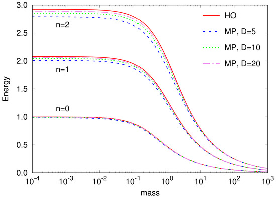
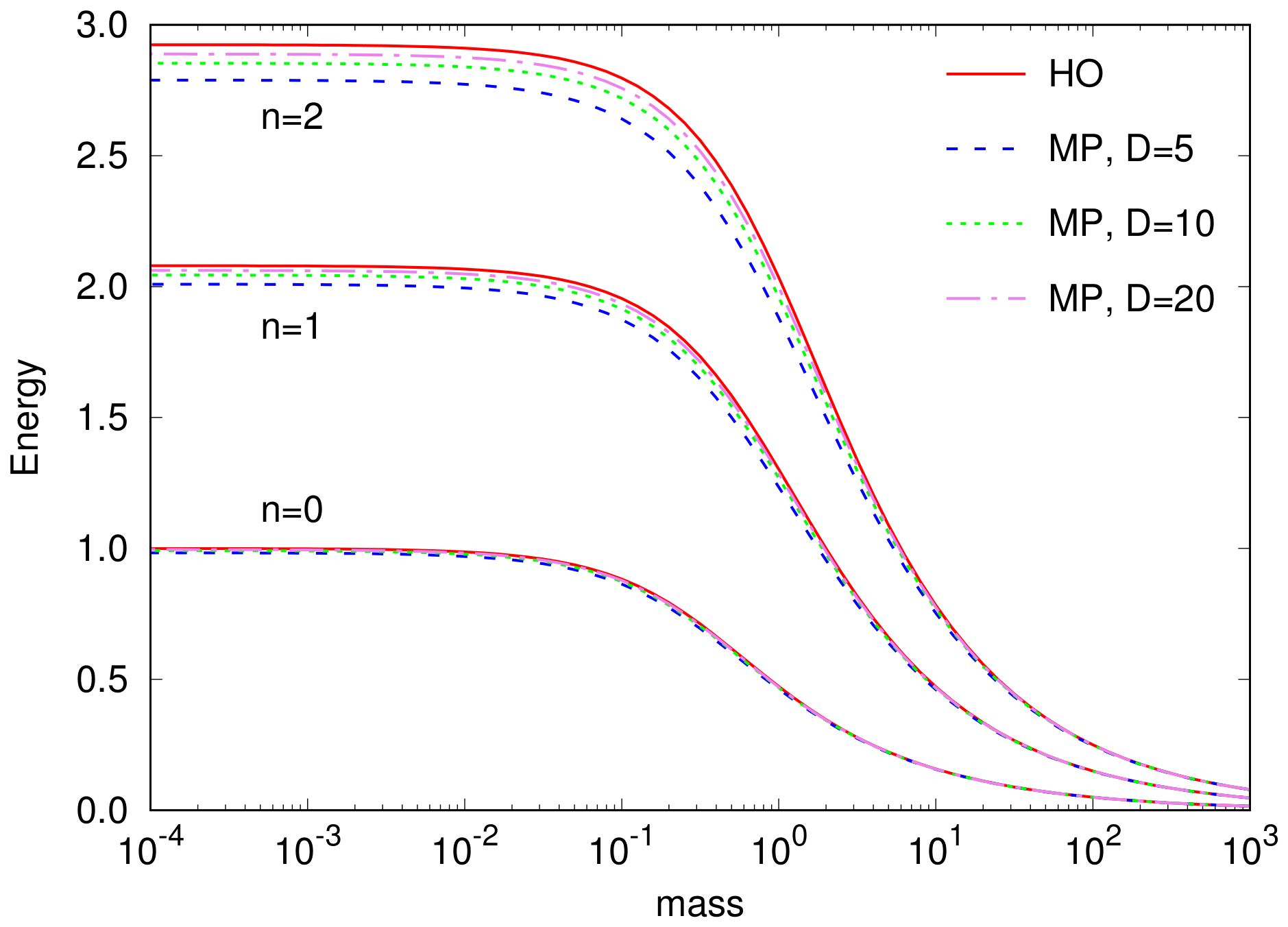
The above behavior with respect to m can be observed in Table 1 but is perhaps better illustrated in Figure 1, which shows the SC-GPPP energies of the first three levels of the $\hslash =k=1$ MP, as a function of m, for three different well depths D. For comparison, the corresponding values for an HO with $k=1$ are also shown. Note that, in addition to manifesting the above mass trends, we observe that as the MP well deepens, the energy values increase, ultimately approaching those of the HO, as expected.

Figure 1. Three lowest-lying energy levels as a function of mass, for $k=1$ MP, with three different well depths. The corresponding energy values for $k=1$ HO [14] are included for comparison. All the values were obtained with the SC-GPPP method. Units where $\hslash =c=1$ were assumed.

3.3. Number of SC-GPPP Bound States

It is of interest to derive a general expression, similar to Equation (28), for the number of allowed SC-GPPP bound states for a particle in an MP. First, note that from Equation (34) and previous discussion on the non-relativistic MP, for $E_{\mathrm{M},n}<D$, it is required that $E_{\mathrm{H},n}<2D$. Then, by setting $E_{\mathrm{H},n}=2D$ in Equation (39) and solving for n, we obtain the Equation (28) expression for $n_{\max }$. However, as discussed above, this expression is not valid in the present relativistic description, which predicts bound states even when $m=0$.

The correct way to obtain the desired expression should involve a counting of the number of real roots of Equation (39) for given values of m, k, and D. Thus, consider the polynomial,

$$P\left(E\right)=E^4-2D{E}^3-8Dm{E}^2+8D{\left(n+{\displaystyle \frac{1}{2}}\right)}^2{\hslash }^{2}k,$$

(40)

with parameters $D,k>0$; $m\ge 0$; and $n=0,1,2,\dots$. This polynomial has two critical points in the non-negative real E-axis: one at the origin, and the other at

$$E_{*}={\displaystyle \frac{3D}{4}}\left(\sqrt{1+{\displaystyle \frac{64m}{9D}}}+1\right).$$

(41)

The latter critical point is a local energy minimum, for all values of $m\ge 0$, while the former is a local maximum for $m>0$, which becomes an inflection point when $m=0$. Note that $P\left(0\right)>0$, while $P\left(E_{*}\right)$ can be positive or negative, depending on n, for given values of $D,k$, and m.

From Equation (41), the minimum $E_{*}$ shifts towards larger values as m increases, such that $E_{*}=2D$ when $m=D/4$. For larger m values, $E_{*}$ lies outside the interval $[0,2D]$, indicating that for $m\ge D/4$, the largest n for which $P\left(E\right)$ still has a root in the interval $[0,2D]$ follows from the condition $P\left(2D\right)=0$. But this leads exactly to Equation (28) for the non-relativistic $n_{\max }$. Thus, for m greater than or equal to one-quarter of the MP well depth, the number of SC-GPPP levels coincides exactly with the non-relativistic number.

On the other hand, for $m<D/4$, the SC-GPPP $n_{\max }$ values start to deviate from Equation (28). In this case, $E_{*}$ lies in the interval $[0,2D]$, and it is necessary that $P\left(E_{*}\right)\le 0$ for there to be a root of the polynomial in the interval, considering that $P\left(0\right)$ is always a positive number. In this case, the largest n for which $P\left(E\right)$ still has a root in the interval $[0,2D]$ follows from the condition $P\left(E_{*}\right)=0$. This leads to the equation

$$n_{\max }=⌊{\displaystyle \frac{\sqrt{8Dm{E}_{*}^2+2D{E}_{*}^3-E_{*}^4}}{\hslash 2\sqrt{2Dk}}}-{\displaystyle \frac{1}{2}}⌋,$$

(42)

which is only valid in the mass range $0\le m<D/4$.

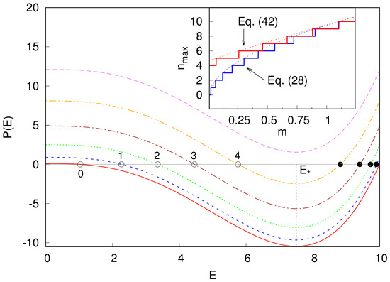
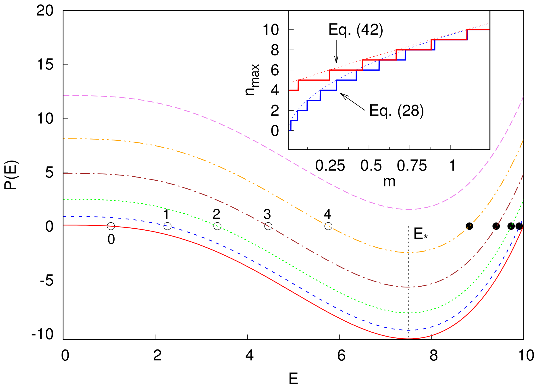
Figure 2 shows the first six profiles of $P\left(E\right)$ for $n=0,1,\dots ,5$, with $\hslash =k=1$, $D=5$, and $m={10}^{-4}$. The roots of the polynomial, corresponding to the values of $E_{\mathrm{H},n}$, are indicated with empty points. In this case, the MP has five levels, with energies given in the first row of Table 1. Note the absence of the sixth level, because $P\left(E\right)$ does not have a root in the interval for $n=5$. The roots above $E_{*}$, indicated with black solid points, do not correspond to valid energy values and should be discarded. The inset of the figure shows the profiles of Equations (28) and (42), in the interval of $0\le m\le D/4$, for an MP with $k=1$ and $D=5$. From the inset of the figure, for the $k=1,D=5$ MP, there are five levels $n_{\max }=4$ at $m=0$. For an arbitrary MP, the maximum number of ultra-relativistic energy levels can be obtained by setting $m=0$ and $E_{*}=3D/2$ in Equation (42), thus leading to,

$$n_{\max }=⌊{\displaystyle \frac{3\sqrt{3}}{8\sqrt{2}}}{\displaystyle \frac{D^{3/2}}{\hslash k^{1/2}}}-{\displaystyle \frac{1}{2}}⌋=⌊{\displaystyle \frac{3\sqrt{3}}{16}}{\displaystyle \frac{D}{\hslash \alpha }}-{\displaystyle \frac{1}{2}}⌋.$$

(43)

Interestingly, in the ultra-relativistic limit, the number of bound states is proportional to both the MP well depth and its width.

Figure 2. First six ($n=0,\dots ,5$) profiles of the polynomial of Equation (40) as a function of E, in the interval $0\le E\le 2D$, for $k=1$, $m=0.0001$, and $D=5$. The empty dots correspond to the roots of $P\left(E\right)$ or the solutions $E_{\mathrm{H},n}$ of Equation (39). The inset shows the profiles of Equations (28) and (42), in the interval of $0\le m\le D/4$, for an MP with $k=1$ and $D=5$. Units where $\hslash =c=1$ were assumed.

Finally, one can easily derive an equation to directly obtain the eigenvalues $E_{\mathrm{M},n}$ by noting that, from Equation (34), for a given $E_{\mathrm{M},n}$, the corresponding value $E_{\mathrm{H},n}$ will be,

$$E_{\mathrm{H},n}=2D\left(1-\sqrt{1-{\displaystyle \frac{E_{\mathrm{M},n}}{D}}}\right).$$

(44)

Then, combining Equations (34), (37), and (44), one obtains

$$\begin{array}{cc}\hfill E_{\mathrm{M},n}={\displaystyle \frac{{\mathcal{E}}_{\mathrm{H},n}}{\sqrt{1+{\displaystyle \frac{1}{2m}}\left[E_{\mathrm{M},n}-D\left(1-\sqrt{1-{\displaystyle \frac{E_{\mathrm{M},n}}{D}}}\right)\right]}}}& -\\ \hfill {\displaystyle \frac{{\mathcal{E}}_{\mathrm{H},n}^2/4D}{1+{\displaystyle \frac{1}{2m}}\left[E_{\mathrm{M},n}-D\left(1-\sqrt{1-{\displaystyle \frac{E_{\mathrm{M},n}}{D}}}\right)\right]}},& \end{array}$$

(45)

which tends to Equation (18) for the HO when $D\to \infty$, as expected.

Note that the corresponding function $f_{\mathrm{M},n}\left(E\right)$ of Equation (45) has a more complicated behavior than $f_{\mathrm{H},n}\left(E\right)$, with more than one fixed point in the domain $[0,D]$, below a certain critical mass. Consequently, even more care should be taken to ensure that the fixed-point iteration $E^{\left(s\right)}=f_{\mathrm{M},n}\left[E^{(s-1)}\right]$ converges to the correct value. In practice, however, there is no need to actually iterate the $f_{\mathrm{M},n}\left(E\right)$ solution directly—since this can always be obtained from the $f_{\mathrm{H},n}\left(E\right)$ fixed-point solution.

4. Approximate WKB and “Exact” Numerical Solutions

4.1. WKB Method

Within the WKB approximation [24,25,26,27], the classical Hamiltonian contours of Equation (7) with the MP given by Equation (2), and energy E, are found to be

$$p\left(x\right)=\pm \sqrt{\left[E-D{\left(1-e^{-\alpha x}\right)}^2\right]\left[E+2m-D{\left(1-e^{-\alpha x}\right)}^2\right]}.$$

(46)

Integrating the above function between the classical turning points, $x_{\mathrm{tp}}=-\ln (1\pm \sqrt{E/D})/\alpha$, leads to the phase space volume $S\left(E\right)$ and the eigenenergies, from the usual half-integer quantized action values, $S_n=2\pi \hslash (n+1/2)$. For an arbitrary finite value of m, the integral over x of Equation (46) can only be performed numerically. On the other hand, an analytical expression can be obtained, for the ultra-relativistic $m=0$ limit, with the Hamiltonian contour adopting the form,

$$p\left(x\right)=\pm \left[E-D{\left(1-e^{-\alpha x}\right)}^2\right],$$

(47)

thus leading to the requisite classical action–energy relationship,

$$S\left(E\right)={\displaystyle \frac{2}{\alpha }}\left[\left(D-E\right)\ln {\displaystyle \frac{\sqrt{D}-\sqrt{E}}{\sqrt{D}+\sqrt{E}}}+2\sqrt{ED}\right].$$

(48)

Note that for $D\to \infty$, the above ultra-relativistic classical action for the MP approaches the ultra-relativistic action of the HO [14], i.e.,

$$S\left(E\right)={\displaystyle \frac{8}{3}}\sqrt{2}\left({\displaystyle \frac{E^{3/2}}{k^{1/2}}}\right),$$

(49)

with $k=2D{\alpha }^2$.

Equation (48) cannot be inverted to obtain a closed-form expression for the WKB energies, but the equation $S_n\left(E\right)=2\pi \hslash (n+1/2)$ can be easily solved numerically. The WKB energy values for the general mass-dependent case were evaluated using a golden-section search method, with the integral numerically evaluated via recursive adaptive Lobatto quadrature.

4.2. “Exact” Numerical Method

Numerical solutions of Equation (7), using the MP of Equation (2), were obtained using the same method reported in Ref. [14] for the HO. The method consists of expanding Equation (7) in a particle-in-a-box basis set, in term of which the kinetic energy matrix representation becomes diagonal and positive-definite. Likewise, the matrix representation of the Morse potential energy—though not diagonal—is nevertheless exact, involving integrals of exponential times trigonometric functions, which can be solved analytically. Using this exact representational method, a perfectly variational convergence with increasing basis size is obtained.

The basis functions used are as follows:

$${\varphi }_N\left(x\right)=\left\{\begin{array}{cc}\sqrt{{\displaystyle \frac{2}{L}}}\sin (N\pi x/L)\hfill & \mathrm{for}N\mathrm{even}\hfill \\ \sqrt{{\displaystyle \frac{2}{L}}}\cos (N\pi x/L)\hfill & \mathrm{for}N\mathrm{odd}\hfill \end{array}\right.$$

(50)

Here, L denotes the width of the box, and $N=1,2,\dots$ runs over the particle-in-a-box eigenstates. In terms of the above basis, the matrix representation of the kinetic energy operator is diagonal, with matrix elements, $K_{NN}$, given by

$$K_{NN}=m\sqrt{1+{\left({\displaystyle \frac{N\pi \hslash }{mL}}\right)}^2}-m.$$

(51)

For a set of mass values lying in the interval ${10}^{-4}\le m\le {10}^3$, the eigenvalues of the matrix $H_{N{N}^{\prime }}=K_{N{N}^{\prime }}{\delta }_{N{N}^{\prime }}+V_{N{N}^{\prime }}$ were computed using a FORTRAN code of the Jacobi eigenvalue algorithm [28]. For all reported energy levels, the box width L and basis size $N_{\max }$ were increased independently until numerical differences were smaller than ${10}^{-6}$. Unlike the HO potential, quadratic in x, the MP is asymmetrical about the origin: $V(x\to -\infty )\to \infty$ and $V(x\to +\infty )\to D$. Consequently, the box was initially placed asymmetrically with respect to $x=0$, such that $L=x_{\max }+\mid x_{\min }\mid$, with $V(x_{\min }<0)=100D$ and $V(x_{\max }\gg 1)\sim {10}^{-6}$. Note that in the increasingly “anharmonic” relativistic limit, numerical convergence becomes increasingly difficult.

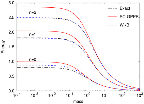
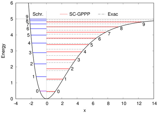
Figure 3 shows a comparison of the lowest three energy levels as a function of m, calculated using the “Exact”, SC-GPPP, and WKB methods, for an MP with $k=m=1$ and $D=10$. The same energy values for selected masses are shown in Table 2. As observed in the previous publication for the HO [14], the SC-GPPP results always turn out to be an overestimate, and the discrepancy increases with increasing n and decreasing m. This is clearly illustrated, also, in Figure 4, where the energy levels obtained from the Schrödinger equation for a $k=m=1,D=5$ MP are placed side by side with those computed with the SC-GPPP method and the exact relativistic numerical solution. Note that for the MP of Figure 4, the SC-GPPP method led to the same number of allowed energy levels as for the non-relativistic case, in accordance with $n_{\max }=9$ from Equation (42). Here, the nth SC-GPPP level is always below the Schrödinger value, as expected from Equation (45), whereas the exact numerical method leads to even lower energy-level values, with at least 14 levels supported by the MP potential well.

Figure 3. Comparison of three lowest-lying energy levels of the $k=1,D=5$ MP system, as a function of mass, as computed using the following: exact numerical method (black dash-dotted lines); SC-GPPP method (red solid lines); WKB method (blue dashed lines). Units where $\hslash =c=1$ were assumed.

Table 2. Comparison of selected energy values for the MP, with $k=1$ and $D=10$.

	$\mathit{n}=0$			$\mathit{n}=1$
$\mathit{m}$	SC-GPPP	WKB	Exact	SC-GPPP	WKB	Exact
$0.0001$	$0.991538$	$0.874670$	$0.799391$	$2.044017$	$1.795132$	$1.808594$
$0.001$	$0.990317$	$0.873766$	$0.798494$	$2.042768$	$1.794223$	$1.807694$
$0.01$	$0.978288$	$0.864976$	$0.789764$	$2.030364$	$1.785354$	$1.798754$
$0.1$	$0.873288$	$0.788545$	$0.718820$	$1.914886$	$1.703301$	$1.714460$
$1.0$	$0.467795$	$0.456901$	$0.436621$	$1.269235$	$1.209206$	$1.205185$
$10.0$	$0.157183$	$0.157024$	$0.156584$	$0.466074$	$0.464740$	$0.464346$
$100.0$	$0.049934$	$0.049932$	$0.049928$	$0.149410$	$0.149397$	$0.149391$
$1000.0$	$0.015805$	$0.015806$	$0.015807$	$0.047378$	$0.047376$	$0.047411$

Figure 4. Schematic representation of the allowed energy levels of the $k=m=1,D=5$ MP systems, as obtained from the Schrödinger solution (Schr.), the SC-GPPP (red solid lines), and exact numerical (black dash-dotted lines) methods. Units where $\hslash =c=1$ were assumed.

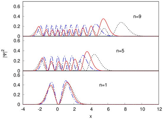
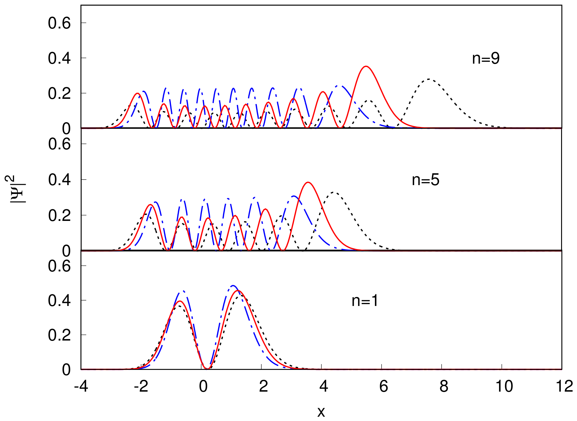
Figure 5 indicates the probability densities of the wavefunction for several different excited eigenstates of the $k=m=1,D=5$ MP—as computed for the non-relativistic, exact numerical relativistic, and SC-GPPP methods. The exact numerical and SC-GPPP eigenstates appear to be more localized in the potential well, due to the larger rescaled mass of the relativistic particle, with the SC-GPPP wavefunction showing a less pronounced compression than that of the exact numerical solution. This trend, also observed for the HO, is related to the “intermediate” role of the SC-GPPP—between the non-relativistic and exact relativistic solutions (and also exhibited in the energy spectrum). Unlike the symmetric harmonic potential, the asymmetrical MP causes the probability density to spread out more toward the dissociation region (larger x), especially for larger excitation numbers n. This feature, well known for the non-relativistic eigenstates, is also observed in the present relativistic description.

Figure 5. Comparison of wavefunction probability densities for several different $k=m=1,D=5$ MP system eigenstates, as computed using the following: exact numerical method (blue dash-dotted lines); SC-GPPP method of Equation (34) (red solid lines); non-relativistic limit (black dotted lines) (color figure online).

The shape of the density plots is also worth commenting on. Given that the SC-GPPP wavefunction is in fact equivalent to a mass-rescaled non-relativistic MP eigenstate, the form of its density is identical to that of the latter—except compressed, in accordance with the larger relativistic effective mass. On the other hand, density plots for the exact numerical solutions are qualitatively different, in that all of the interior peaks are of nearly equal height—as opposed to the familiar non-relativistic form, which drops down gently as one approaches the origin.

The same feature was previously observed in the HO [14] probability densities, and can be attributed to a flattening in the envelope density function, as described within the so-called “bipolar formalism” [29]. The explanation relies on the fact that each “standing-wave” eigenstate solution $\psi \left(x\right)$ comprises two equal and oppositely moving traveling waves, ${\psi }_{\pm }\left(x\right)$, with $\psi \left(x\right)={\psi }_{+}\left(x\right)+{\psi }_{-}\left(x\right)$ [29]. The traveling wave densities, ${\psi }_{\pm }^2\left(x\right)$, are equal and smoothly varying and correspond to the “envelope” of the standing wave. In the classically allowed region of space, these are very nearly inversely proportional to the local classical velocity field, $v\left(x\right)$ [29]. In the relativistic case, the velocity is always smaller than in the non-relativistic case and is, of course, limited by a maximum finite value, c. Relativity thus serves to flatten the variation in the velocity field $v\left(x\right)$—and, thereby, also the corresponding envelope density function.

5. Comparison of Relativistic Harmonic Oscillators

In this section, we present a comparison between the SC-GPPP solutions for a particle in a harmonic oscillator, as discussed in the preceding sections, versus previously reported relativistic HO results obtained using the standard Klein–Gordon equation (i.e, the “KGO”). A similar discussion, for the Morse potential case, will be presented in an upcoming publication. Such a comparison is vital for really bringing home the reasons why a physically reasonable theory, such as any of the Equation (7)-based methods presented here (including the “worst-case” SC-GPPP approximation), can provide sensible results, even when the “standard” approach cannot.

The one-dimensional KGO can be defined via the equation [6]

$$-{\hslash }^2{\displaystyle \frac{{\partial }^2\mathsf{\Psi }\left(x\right)}{\partial t^2}}=\left(\widehat{P}{\widehat{P}}^{†}+m^2\right)\mathsf{\Psi }\left(x\right),$$

(52)

where $\widehat{P}=\widehat{p}-im\omega x$ and $\widehat{P}†=\widehat{p}+im\omega x$. Note that the KGO is arguably the most favorable possible realization of the HO system within a Klein–Gordon context—certainly much better, e.g., than the disastrous Equation (5) would be. Note that Equation (52) above can be rewritten as

$$-{\hslash }^2{\displaystyle \frac{{\partial }^2\mathsf{\Psi }\left(x\right)}{\partial t^2}}=\left[{\widehat{p}}^2+m^2{\omega }^2{x}^2+m\hslash \omega +m^2\right]\mathsf{\Psi }\left(x\right)$$

(53)

or

$$-{\hslash }^2{\displaystyle \frac{{\partial }^2\mathsf{\Psi }\left(x\right)}{\partial t^{\prime 2}}}=\left[{\displaystyle \frac{{\widehat{p}}^2}{2m}}+{\displaystyle \frac{1}{2}}m{\omega }^2{x}^2+{\displaystyle \frac{\hslash \omega }{2}}+{\displaystyle \frac{m}{2}}\right]\mathsf{\Psi }\left(x\right)$$

(54)

where $t^{\prime }=t\sqrt{2m}$.

Equation (54) admits stationary solutions, for which the time-independent contribution satisfies the following Schrödinger-like equation for a particle in a harmonic potential:

$$\left({\displaystyle \frac{{\widehat{p}}^2}{2m}}+{\displaystyle \frac{1}{2}}m{\omega }^2{x}^2+{\displaystyle \frac{\hslash \omega }{2}}\right)\psi \left(x\right)={\displaystyle \frac{E^2-m^2}{2m}}\psi \left(x\right).$$

(55)

The corresponding energy eigenvalues of the KGO then adopt the form [30]

$$E_{\mathrm{KGO},n}=\sqrt{2m\left({\mathcal{E}}_n+{\displaystyle \frac{\hslash \omega }{2}}\right)+m^2}-m,$$

(56)

where ${\mathcal{E}}_n$ is given by Equation (16) and $E_{\mathrm{KGO},n}$ is the energy of the nth KGO level, not including the relativistic rest energy.

In the non-relativistic limit $m\to \infty$, Equation (55) approaches the Schrödinger equation for a particle in a harmonic potential, apart from a constant energy shift of $\hslash \omega /2$. This is the main reason why this model is considered a relativistic limit for a spin-0 particle in a harmonic potential [6]. Indeed, the ansatz$(\widehat{p}-im\omega x)$ is just a suitable “non-minimal coupling”, which leads to the desired particle-in-a-potential problem, in the same way that the problem of a particle in an electromagnetic potential is incorporated by making the usual minimal substitution ${\widehat{p}}_{\mu }-e{A}_{\mu }$ [1,2].

On the other hand, an alternative KGO equation is obtained if the operator ordering ${\widehat{P}}^{†}\widehat{P}$ is used in Equation (52), thus leading to the time-independent equation

$$\left({\widehat{P}}^{†}\widehat{P}+m^2\right)\psi \left(x\right)=E^2\psi \left(x\right),$$

(57)

or

$$\left({\displaystyle \frac{{\widehat{p}}^2}{2m}}+{\displaystyle \frac{1}{2}}m{\omega }^2{x}^2-{\displaystyle \frac{\hslash \omega }{2}}\right)\psi \left(x\right)={\displaystyle \frac{E^2-m^2}{2m}}\psi \left(x\right),$$

(58)

with energy values

$$E_{\mathrm{KGO},n}=\sqrt{2m\left({\mathcal{E}}_n-{\displaystyle \frac{\hslash \omega }{2}}\right)+m^2}-m.$$

(59)

Note that from Equations (55) and (58), the Hamiltonians,

$${\widehat{H}}_{\pm }={\displaystyle \frac{{\widehat{p}}^2}{2m}}+{\displaystyle \frac{1}{2}}m{\omega }^2{x}^2\pm {\displaystyle \frac{\hslash \omega }{2}}$$

(60)

are isospectral with the Schrödinger Hamiltonian for a particle in a harmonic oscillator, apart from an additional vanishing eigenvalue. Consequently, ${\widehat{H}}_{+}$ and ${\widehat{H}}_{-}$ are the partners of the harmonic oscillator Hamiltonian, in the sense of supersymmetric quantum mechanics (SUSY-QM) [31,32,33,34].

Within the SUSY-QM formalism, the operator $\widehat{Q}=\widehat{P}/\sqrt{2m}$ corresponds to the supercharge operator, considering that it yields the superalgebra [31,32],

$${\mathcal{H}}^{\mathrm{HO}}={\displaystyle \frac{1}{2}}\{\widehat{Q},{\widehat{Q}}^{†}\},$$

(61)

where ${\mathcal{H}}^{\mathrm{HO}}$ is the Schrödinger harmonic oscillator Hamiltonian and $\{·\}$ the anticommutator. The corresponding SUSY partner potentials are

$$V_{\pm }={\displaystyle \frac{1}{2}}m{\omega }^2{x}^2\pm {\displaystyle \frac{\hslash \omega }{2}},$$

(62)

which, in terms of the so-called superpotential W, adopt the general form [31,32],

$$V_{\pm }=W^2\pm {\displaystyle \frac{\hslash }{\sqrt{2m}}}{\displaystyle \frac{dW}{dx}}.$$

(63)

It is easy to verify that, for the harmonic oscillator, W takes the form

$$W=\sqrt{{\displaystyle \frac{m}{2}}}\omega x.$$

(64)

The above discussion suggests that the non-minimal coupling of Equation (1) in the free-particle KG equation, introduced to define the KGO model, could be extended to an arbitrary potential within the SUSY-QM formalism [31]. Note that this approach is only valid for shape-invariant potentials—i.e., those for which the corresponding Schrödinger Hamiltonian has a supersymmetric partner [31,32]. Most of the potentials taught in introductory quantum mechanics courses are potentials of this type.

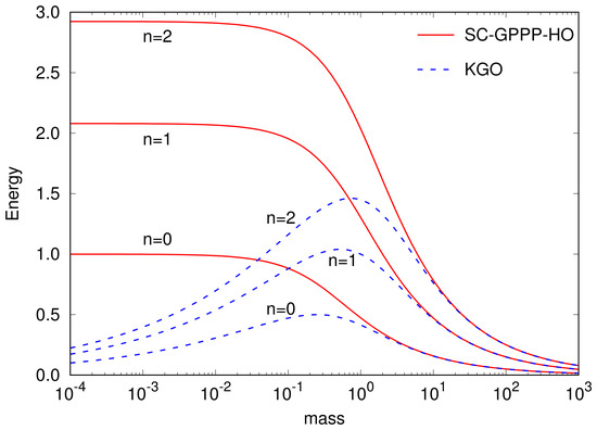
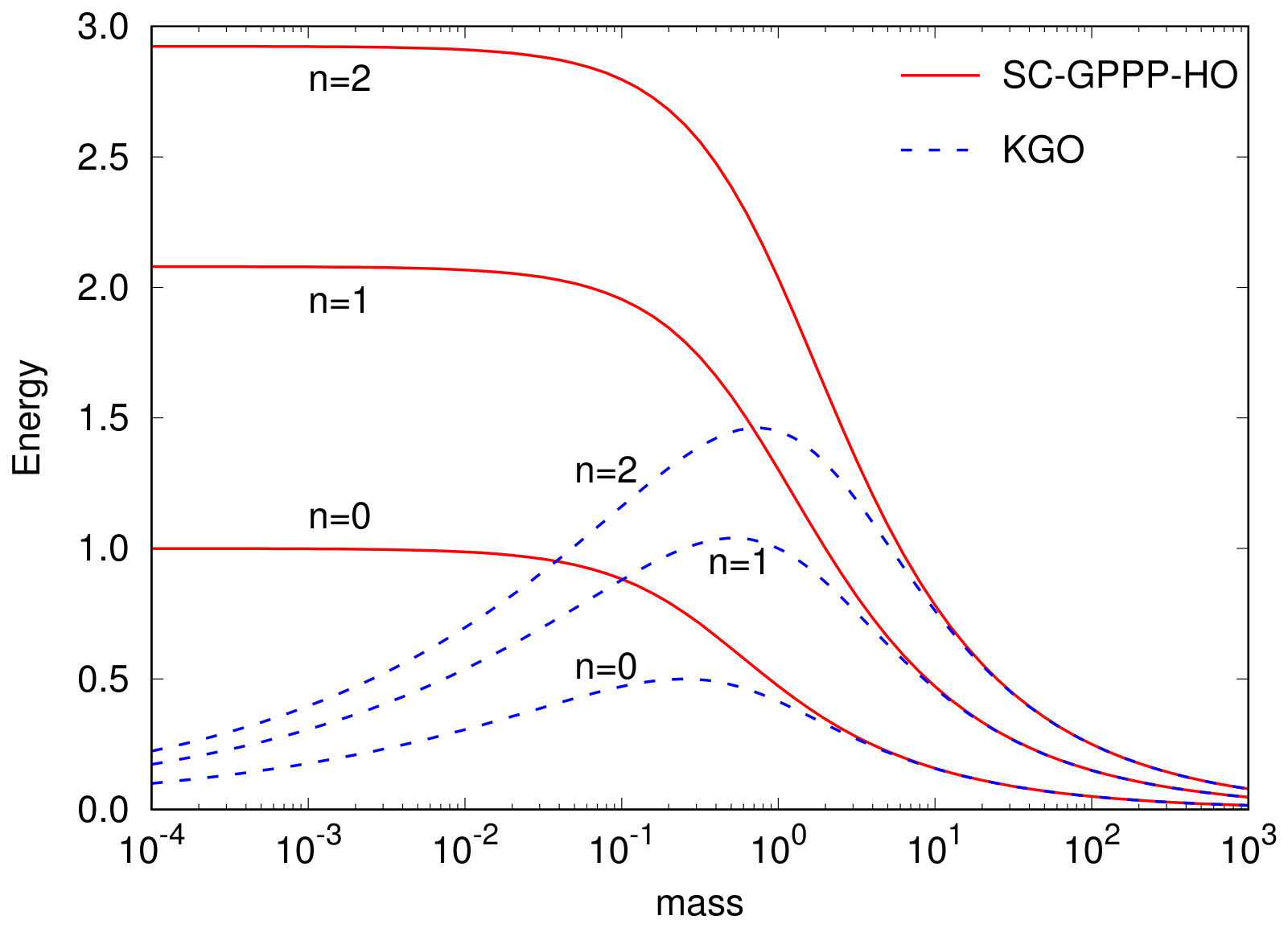
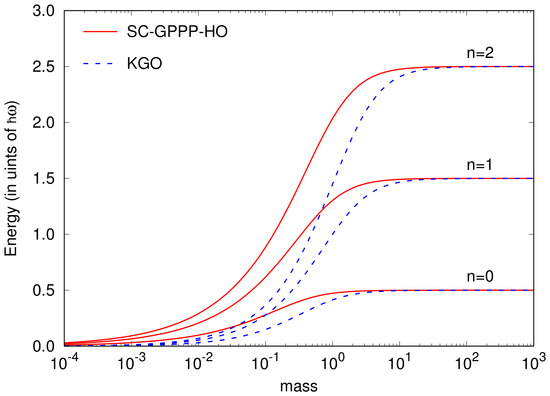
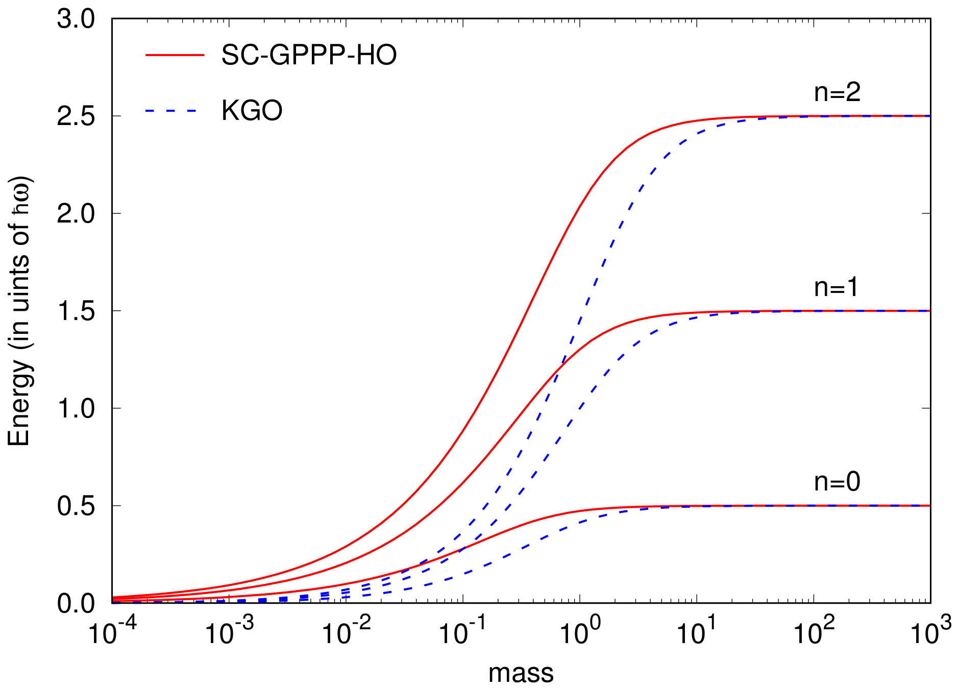
At present, however, the relevant question is whether the KGO oscillator model is the correct relativistic generalization of a particle in a harmonic potential. Although this model turns out to predict truly bound states, which approach the correct non-relativistic limit, a couple of points appear obscure in this formulation. First, the KGO wavefunctions are exactly the Hermite-polynomial-based Schrödinger solutions for the HO. That is, the KGO model predicts that the particle eigenstates remain unchanged—no matter how far the system moves toward the ultra-relativistic limit. Second, consider how the KGO eigenenergies change in the ultra-relativistic limit. This is indicated in Figure 6 and Figure 7, where the first three energy values of the KGO are compared with the corresponding SC-GPPP energies, as a function of m. Note that the dashed curves in Figure 6 and Figure 7 correspond to the KGO expression,

$$E_{\mathrm{KGO},n}=\sqrt{2m{\mathcal{E}}_n+m^2}-m,$$

(65)

where the level shift $\pm \hslash \omega /2$ has been removed from Equations (56) or (59) to better illustrate the comparison in the non-relativistic limit.

Figure 6. Comparison of three lowest-lying energy levels of the $k=1$ HO system, as a function of mass, as computed using the SC-GPPP method and the values obtained from Equation (65) for the Klein–Gordon oscillator. Units where $\hslash =c=1$ were assumed.

Figure 7. The same plot as in Figure 6 but with the vertical axis in units of $\hslash \omega$.

From the figures, it is clear that when $m\to \infty$, both methods approach the correct non-relativistic energy values. However, when approaching the ultra-relativistic limit, the KGO energies reach a maximum and then steadily diminish, approaching zero as $m\to 0$. Such behavior, as discussed, is simply unphysical and will not properly describe massless particles.

6. Conclusions

In its first application to the quantum harmonic oscillator, the (SC)GPPP method proved to be a promising alternative approach for easily extending well-known problems in quantum mechanics to the relativistic limit. By using a continued-fraction representation of the square-root kinetic energy operator, the method allows for a practical treatment of the square-root operator that is even Schrödinger-like. Thus, starting from the well-known non-relativistic solution, the (SC)GPPP solutions to the harmonic oscillator problem turned out to be smooth, well behaved, and fully analytical over the entire range of system parameters, from the non-relativistic to the relativistic limit.

Taking it a step further, the Morse potential provides the next non-harmonic generalization, as the quintessential model for describing covalently bounded molecules in a more realistic way. As such, the problem of a particle in a Morse potential is one of those that has a Schrödinger analytical solution; therefore, one would also expect a closed-form solution within the Schrödinger-type-(SC)GPPP approach. However, as shown in the above results, the present application of the method exceeded our expectations. The simple formulas—and combinations of formulas—that emerge, along with the smoothness of their behavior at various limits, including the harmonic limit, lead us to conclude that the (SC)GPPP is a straightforward method that provides analytical solutions and easy-to-understand trends! It is worth noting the derivation of formulas for calculating the number of allowed energy levels in the Morse potential well for all values of the relativistic parameter m. Thus, the maximum number of ultra-relativistic energy levels increases linearly with the well depth, at a rate faster than the sub-linear $\sim D^{1/2}$ power law observed in the non-relativistic limit. On the other hand, the approximated WKB and “exact numerical” methods, previously developed in the context of the harmonic potential problem, have been readily applied to the particle in the Morse potential. As with the harmonic oscillator case, all these methods show good agreement with each other along the entire mass range.

Of course, given its “usual” molecular physics application, one might well wonder if a relativistic generalization of the MP is indeed useful in this context. To this end, we consider the relativistic corrections to the vibrational energy levels of H₂—arguably the most “relativistic” diatomic molecule (at least in terms of the lowest-lying vibrational bound states). For this system, best-fit Morse parameters are found to be $D=4.7446$ eV, $\alpha =1.9425$ Å, and $m=0.5039$ amu, leading to relativistic corrections to the vibrational energy levels on the order of ten thousandths of a wavenumber. While such small differences are at the edge of what can be achieved experimentally using modern spectroscopic techniques (and are accordingly of great interest in so-called “ultra-high precision” spectroscopy experiments designed to test the fundamental laws of nature), there is no question but that the Morse potential model itself is nowhere near this accurate a model of the actual H₂ vibrational potential. Since relativistic corrections manifest as energy “shifts” rather than say, spectroscopic energy splittings, the present results cannot hope to settle any questions pertaining to the physically “correct” relativistic generalizations—at least not in the molecular physics context. Nevertheless—and as discussed in Section 1—there are already some realistic scenarios where relativistic effects for the MP system may manifest. These may include, for instance, highly energetic relativistic electrons, manifesting transitions in the extreme ultraviolet range, i.e., around $\hslash \omega \approx 100$ eV. Such energies are feasibly significant on the scale of the electron rest energy of 511 keV. In such contexts, the MP may be significant as a model for finite spectra, which give rise to so-called “Schottky anomalies” [11].

Finally, the previous section presents a comparison between the results of the SC-GPPP for the harmonic oscillator and those obtained for the so-called Klein–Gordon oscillator. The comparison reveals that the energy levels of the KGO do not properly describe the ultra-relativistic limit, with the energy levels approaching zero as $m\to 0$. An interesting finding concerns the relationship between the KGO model and supersymmetric quantum mechanics. This and others features of this model will be addressed in a future work.

References

- Moshinski, M.; Szczepaniak, A. The Dirac oscillator. J. Phys. A Math. Gen. 1989, 22, L817–L819. [Google Scholar] [CrossRef]
- Bruce, S.; Minning, P. The Klein-Gordon oscillator. Il Novo C. 1993, 106, 711–713. [Google Scholar] [CrossRef]
- Martínez-y-Romero, R.P.; Núñez-Yépez, H.N.; Salas-Brito, A.L. Relativistic quantum mechanics of a Dirac oscillator. Eur. J. Phys. 1995, 16, 135–141. [Google Scholar] [CrossRef]
- Rozmej, P.; Arvieu, R. The Dirac ocsillator. A relativistic version of the Jayme-Cummings model. J. Phys. A Math. Gen. 1999, 32, 5367–5382. [Google Scholar] [CrossRef]
- Franco-Villafañe, J.A.; Sadurni, E.; Barkhofen, S.; Kuhl, U.; Mortessagne, F.; Seligman, T.H. First Experimental Realization of the Dirac Oscillator. Phys. Rev. Lett. 2013, 111, 170405. [Google Scholar] [CrossRef] [PubMed]
- Mirza, B.; Mohadesi, M. The Klein Gordon and the Dirac Oscillators in a Noncommutative Space. Commun. Theor. Phys. 2004, 42, 664–668. [Google Scholar] [CrossRef]
- Carvalho, J.; Carvalho, A.M.d.M.; Cavalcante, E.; Furtado, C. Klein–Gordon oscillator in Kaluza–Klein theory. Eur. Phys. J. C 2016, 76, 365. [Google Scholar] [CrossRef]
- Morse, P. Diatomic molecules according to the wave mechanics. II. Vibrational levels. Phys. Rev. 1929, 34, 57–64. [Google Scholar] [CrossRef]
- Sierra-Suarez, J.A.; Majumdar, S.; McGaughey, A.J.H.; Malen, J.A.; Higgs, C.F., III. Morse potential-based model for contacting composite rough surfaces: Application to self-assembled monolayer junctions. J. App. Phys. 2016, 119, 145306. [Google Scholar] [CrossRef]
- LeRoy, R.J.; Dattani, N.S.; Coxon, J.A.; Ross, A.J.; Cozet, P.; Linton, C. Accurate analytic potentials for Li2(X1) and Li2(A1) from 2 to 90 Å, and the radiative lifetime of Li(2p). J. Chem. Phys. 2009, 131, 204309. [Google Scholar]
- Gomez, I.S.; Santos, E.S.; Abla, O. Morse potential in relativistic contexts from generalized momentum operator: Schottky anomalies, Pekeris approximation and mapping. Mod. Phys. Lett. A 2021, 36, 2150140. [Google Scholar] [CrossRef]
- Strange, P. Relativistic Quantum Mechanics: With Applications in Condensed Matter and Atomic Physics, 1st ed.; Cambridge University Press: New York, NY, USA, 1998; pp. 64–98. [Google Scholar]
- Grave de Peralta, L.; Poveda, L.A.; Poirier, B. Making relativistic quantum mechanics simple. Eur. J. Phys. 2021, 42, 055404. [Google Scholar] [CrossRef]
- Poveda, L.A.; Grave de Peralta, L.; Pittman, J.; Poirier, B. A Non-relativistic Approach to Relativistic Quantum Mechanics: The Case of the Harmonic Oscillator. Fund. Phys. 2022, 52, 29. [Google Scholar] [CrossRef]
- Grave de Peralta, L. Did Schrödinger have other options? Eur. J. Phys. 2020, 41, 065404. [Google Scholar] [CrossRef]
- Klein, O. Quantentheorie und fünfdimensionale Relativitätstheorie. Z. Phys. 1926, 37, 895–906. [Google Scholar] [CrossRef]
- Gordon, W. Der Comptoneffekt nach der Schrödingerschen Theorie. Z. Phys. 1926, 40, 117–133. [Google Scholar] [CrossRef]
- Dirac, P.M. The Quantum Theory of the Electron. Proc. R. Soc. Lond. A 1928, 117, 610–624. [Google Scholar] [CrossRef]
- Moreau, W.; Easter, R.; Neutze, R. Relativistic (an)harmonic oscillator. Am. J. Phys. 1994, 62, 531–535. [Google Scholar] [CrossRef]
- Dahl, J.P.; Springborg, M. The Morse oscillator in positon space, momentum space, and phase space. J. Chem. Phys. 1988, 88, 4535–4547. [Google Scholar] [CrossRef]
- Born, M.; Oppenheimer, R. Zur Quantentheorie der Molekeln. Ann. Phys. 1927, 84, 457–484. [Google Scholar] [CrossRef]
- Feynman, R. Force in molecules. Phys. Rev. 1939, 56, 340–343. [Google Scholar] [CrossRef]
- Tipping, R.H.; Ogilvie, J.F. Expectation values for Morse oscillator. J. Chem. Phys. 1983, 76, 2537–2540. [Google Scholar] [CrossRef]
- Fröman, N.; Fröman, P.O. JWKB Approximation; North-Holland: Amsterdam, The Netherlands, 1965. [Google Scholar]
- Littlejohn, R.G. Phase Space WKB. Phys. Rev. Lett. 1985, 54, 1742. [Google Scholar] [CrossRef] [PubMed]
- Brack, M.; Bhaduri, R.K. Semiclassical Physics; Addison-Wesley: Boston, MA, USA, 1997. [Google Scholar]
- Semay, C.; Ducobu, L. Quantum and classical probability distributions for arbitrary Hamiltonians. Eur. J. Phys. 2016, 37, 045403. [Google Scholar] [CrossRef]
- Golub, G.H.; Van Loan, C.F. Matrix Computations, 3rd ed.; The Johns Hopkins University Press: Baltimore, MD, USA, 1996. [Google Scholar]
- Poirier, B. Reconciling semiclassical and Bohmian mechanics. I. Stationary states. J. Chem. Phys. 2004, 121, 4501. [Google Scholar] [CrossRef] [PubMed]
- Rao, N.A.; Kagali, B.A. Energy profile of the one-dimensional Klein–Gordon oscillator. Phys. Scr. 2008, 77, 015003. [Google Scholar] [CrossRef]
- Cooper, F.; Khare, A.; Sukhatme, U. Supersymmetry and quantum mechanics. Phys. Rep. 1985, 251, 267–385. [Google Scholar]
- Sukumar, C.V. Supersymmetric quantum mechanics of one-dimensional systems. J. Phys. A Math. Gen. 1985, 18, 2917–2936. [Google Scholar] [CrossRef]
- Pursey, D.L. Isometric operators, isospectral Hamiltonians, and supersymmetric quantum mechanics. Phys. Rev. D 1986, 33, 2267–2279. [Google Scholar] [CrossRef]
- Gendenshtein, L.E. Derivation of exact spectra of the Schrödinger equation by means of supersymmetry. JEPT Lett. 1984, 38, 356–359. [Google Scholar]
Disclaimer/Publisher’s Note: The statements, opinions and data contained in all publications are solely those of the individual author(s) and contributor(s) and not of MDPI and/or the editor(s). MDPI and/or the editor(s) disclaim responsibility for any injury to people or property resulting from any ideas, methods, instructions or products referred to in the content. |
© 2026 by the authors. Licensee MDPI, Basel, Switzerland. This article is an open access article distributed under the terms and conditions of the Creative Commons Attribution (CC BY) license.