


Abstract
Resonant Vacuum Theory (RVT) is a working hypothesis in which matter consists of topologically bound solitons in a single nonlinear vacuum medium that also carries light; the electron is a closed, framed soliton, and the atomic field is a physical standing wave, not a probability amplitude. For hydrogen, this paper takes three steps. First, a closure model: the standing envelope wave on the core line carries integer azimuthal and radial node counts , and minimizing the classical shell energy at fixed reconstructs the Bohr levels Hartree. This is the Bohr–Sommerfeld condition in field language, with ℏ, , and as stated inputs. Second, a Cartesian 3D calibration of the linear envelope sector: the proton potential comes from the lattice Gauss equation and the stationary Klein–Gordon equation is solved without spherical harmonics, angular projectors, or values of ℓ; at every resolution the fourteen lowest modes carry the ; ; content (multiplicities 1, 4, 9), and under refinement their frequencies converge to the Coulomb shell values (extrapolated within of the exact Klein–Gordon–Coulomb level). Third, a consistency test fixes what the classical field can be: letting the envelope source the Gauss equation with its own unit Noether charge reduces the binding from to Hartree and removes the ladder, so an uncompensated envelope cannot be the electron’s charge distribution. The reading adopted is therefore that the charge resides in a compact core and the atomic field is a neutral standing wave that guides it; the external-field calculation is what that reading amounts to at this level, and the coupled core–field dynamics remain the next test.
1. Introduction
The hydrogen spectrum, the series of discrete energy levels , is one of the most precisely measured and successfully predicted phenomena in physics. Quantum mechanics derives it from the Schrödinger equation with a Coulomb potential, yielding the full classification of states and their energies. This derivation is correct, but it treats the electron as a point particle described by a complex wavefunction whose squared modulus gives a probability density.
An alternative tradition, stretching from Bohr and Sommerfeld through de Broglie to modern soliton models, asks whether the discrete spectrum can arise from geometric or topological constraints on an extended, classical configuration, without invoking a probabilistic wavefunction. Within this tradition, Rybakov and Saha [1,2] gave an explicit Einstein–de Broglie soliton model of hydrogen in which a time-harmonic soliton bound to a Coulomb center moves on a stationary orbit of Bohr-radius size without radiating; the present work is a minimal geometric variant of that program, and its relation to it is set out in Section 7. The Bohr–Sommerfeld quantization condition is the prototype of the whole approach: a classical orbit is quantized by requiring an integer number of de Broglie wavelengths along its circumference.
This paper presents a geometric model of the hydrogen atom within Resonant Vacuum Theory [3,4], a working hypothesis in which the vacuum is a single classical nonlinear medium with a mass gap, and matter particles are candidate topological solitons of that medium. The gap frequency is the resonance the name refers to. In this paper its identification with the Compton frequency is an input (Section 2 and Section 2.3), not a result. In this framework, the electron is modeled as a closed, framed configuration: a localized core of Hopf charge whose core line carries an internal orientation. For odd the rotation of the whole soliton is a non-contractible loop in configuration space, which supplies the required kinematics [5]; it does not by itself prove the quantum representation , which requires Finkelstein–Rubinstein (FR) quantization of that configuration space [6] and, ultimately, dynamical selection of the non-trivial sector.
What a soliton-atom model is for. Standard quantum mechanics postulates the action quantum, a complex amplitude with a statistical reading, the spin- representation, and exchange antisymmetry, and then derives the atom from them. A soliton-atom model reverses the order. It starts from one deterministic field and asks how much of that list can be recovered as the dynamics of extended objects: the level ladder as a closure (interference) condition on a real field, the orbital shapes as stationary modes of that field, spin as a topological property of the core, and exclusion as a state-dependent interaction between identical solitons. The prize, if the program succeeds, is not a new hydrogen spectrum but one mechanism behind quantities that are separate postulates in the standard account, together with parameter-free corrections wherever an extended core differs from a point charge. The present paper establishes the first two items in their linear, stationary form and states what the remaining items require.
The internal structure of the proton is outside the scope of this atomic reduction. For the three-dimensional orbital gate below, only its conserved gauge charge is used: the static background is calculated from the lattice Gauss equation rather than inserted as an analytic potential.
The central results of this paper are:
- 1.
- Integer closure → Bohr spectrum. The standing wave on the closed core line must close after one circuit, admitting integer azimuthal windings w and radial node counts q; the spin-related statement concerns the rotation of the whole soliton and is separate from this closure. The sum is identified with the principal quantum number, and minimizing a classical shell energy reconstructs Hartree exactly.
- 2.
- Cartesian three-dimensional orbital gate. Solving the classical charged-field equation on a cubic grid produces the ; ; orbital content and its nodal structures without an angular basis supplied to the solver, with frequencies approaching the nonrelativistic Coulomb shell benchmarks under grid refinement. This gate is a calibration: it runs the no-angular-input Cartesian solver on the one case whose answer is known, including the solver’s failure mode at the point-source cusp, so that the same protocol can be trusted in the coupled nonlinear calculation (H3B, Section 7), where the answer is not known.
- 3.
- Explicit calibration. The model exposes precisely which constants (ℏ, , ) are imported through atomic units and marks their derivation as the open challenge.
- 4.
- A consistency test. A charge-normalized Klein–Gordon–Poisson solve (Section 7.4) shows that an uncompensated envelope cannot be the electron’s charge distribution. This fixes the reading of the field and places the charge in a compact core.
What the computed field is. The algebraic closure derivation of the gross spectrum does not solve the Schrödinger eigenvalue equation: it minimizes a classical shell energy over the closure radius. The independent H3A calculation does solve a stationary-mode eigenproblem, but for the classical charged Klein–Gordon field of Equation (9), and in this framework that field is not a probability amplitude. A stationary mode is a standing wave of a field that lives in ordinary three-dimensional space and has a definite value at every point. RVT is a realist, deterministic field theory. This field is a physical standing wave in a nonlinear medium, not a probability amplitude, and the program does not use the probabilistic interpretation: it asks whether the same spectrum follows from a deterministic field, and it treats the quantum-mechanical results as the standard every such attempt must meet. That premise is the model’s starting point, not a result of the paper, and it raises a question the probabilistic reading never meets: a field that is physical must be something definite, either the electron’s charge distribution, or a neutral wave that guides a compact charged core. The two readings are not equivalent. Section 7.4 lets the envelope source the Gauss equation with its own conserved charge and finds that the first reading destroys half the ground-state binding and the ladder with it, while the second is what the external-field calculation of Section 4 amounts to and reproduces the spectrum at this level; how a neutral guiding wave acquires its Coulomb coupling to the proton is part of the coupled problem (H3B). The reading adopted here is therefore the second: the orbital shapes computed below are standing-wave patterns of a linear, neutral guiding field, and the mode intensity is where the compact core is found over time, a distribution that must follow from the coupled dynamics (H3B) and is not derived here. What the calibration tests is whether such a field, given no angular basis, carries the hydrogen shell structure. The calculation is linear and stationary; it derives neither the Born rule nor the statistics of measurements, and it does not show that nature is not probabilistic. Within these limits the model remains classical and geometric while reconstructing the observed gross levels exactly in its pure closure limit.
The paper is organized as follows. Section 2 defines the candidate core and the closure integers. Section 3 derives the shell energy, identifies its Bohr–Sommerfeld content, and shows that it reproduces the gross spectrum. Section 4 gives the Cartesian three-dimensional orbital test. Section 5 states what the stationary calculation does not yet establish about transitions. Section 6 exposes the calibration that hides ℏ, , and in the choice of atomic units. Section 7 separates the achieved linear gate from the open nonlinear problem, reports the self-field test (Section 7.4), and states the criterion that a distinguishing observable must meet.
Terminology. Throughout, the vacuum medium is the classical field of Equation (1) together with the gauge sector of Equation (7); its gap is the resonance the theory is named for; the core is its localized nonlinear configuration, for which the candidate is a Hopf soliton; the framing is the internal orientation transported around the closed core line, which for the core makes one full twist per circuit; the charged envelope is the linear exterior field of the H3A test, minimally coupled to the gauge field and carrying the rest-frame phase (whether it also carries the electron’s charge is tested in Section 7.4, where the answer is negative, so that in the reading adopted here it is the neutral field that guides the core); the closure counts are node counts of the standing envelope wave on the band; and the action cell is the imported unit of action (here ℏ) in which those counts are measured. H3A denotes the stationary linear test of Section 4, and H3B the coupled nonlinear core–envelope–gauge calculation that this paper specifies but does not perform. The soliton atom of Rybakov and Saha [1,2] describes the electron as a time-harmonic soliton of a nonlinear scalar field whose center, in the Coulomb field of the nucleus, moves on a stationary orbit of the order of the Bohr radius without radiating; the present work keeps that stationary ansatz for the envelope, replaces the scalar core by a candidate topological one, and adds the Cartesian no-angular-input test.
2. Candidate Framed Core and Closure Integers
2.1. Candidate Electron Core
The core sector used in the RVT program is not a lone complex scalar with a Mexican-hat potential. Such a statement would not by itself evade Derrick’s scaling obstruction or establish a stable particle [7]. The concrete candidate is instead an amplitude field coupled to an orientation (equivalently a field), with quadratic-gradient, quartic Faddeev–Skyrme, amplitude-gradient, and symmetry-breaking terms [8,9,10,11]. In dimensionless notation its static energy is
where and in lattice units. The quartic term can balance the quadratic term under spatial rescaling; the potential selects the vacuum direction and gives the transverse field the mass gap ; and the map admits an integer Hopf charge . The gap is fixed in lattice units; its relation to the electron mass is not. Identifying the inverse decay length with the inverse reduced Compton wavelength, , imports the measured mass scale, and it becomes a derivation only if a separate dynamical calculation fixes the conversion and shows that this core mode is the envelope’s mass mode; H3A supplies no such calculation. With the amplitude frozen, , Equation (1) is the functional relaxed in the program’s lattice computations [12]. Axisymmetric relaxations of it have produced converged, finite-size cells [13], but they are neither a free three-dimensional existence proof nor the coupled atomic calculation performed below. We therefore call this a candidate electron core throughout.
Its closed core line carries an internal framing. For the core this framing has one full twist (the self-linking of the framed core line is the Hopf charge), so it closes after a single circuit; the loop relevant to spin is not this circuit but the rotation of the whole soliton (Section 2.2). Dynamical survival of this framed core after coupling to the charged envelope is the H3B question, not an assumption hidden inside H3A.
2.2. Framing and the Rotation Loop
The proposed electron core carries an internal orientation inherited from the sector, while the potential selects a vacuum direction. A closed core line is therefore treated as a framed curve, carrying an internal orientation along the loop; in a smooth field that framing twists an integer number of times per circuit, once for the core.
The spin-related topology belongs to the rotations of the whole soliton, not to this ribbon. The rotation group has : a rotation is a non-contractible loop, whereas its double is contractible, and the covering group closes only after . For Hopf solitons the loop in configuration space generated by a rotation is non-contractible exactly when is odd, so only odd- solitons can be quantized as fermions [5]. This is the topology needed to permit a spinorial Finkelstein–Rubinstein quantization [6] (Appendix A); it neither proves spin- nor makes the configuration fermionic, which requires a choice, or a derivation, of the representation on the configuration space. The present closure model selects the odd sector, , as its electron ansatz; for the classical angular momentum that such a core carries when it isorotates, at its half quantum of isospin, see open problem 1 in Section 7.5. Demonstrating that Equation (1) dynamically supports that core once it is coupled to the charged envelope, and then deriving the non-trivial quantum representation on its configuration space, remain separate open tests. No energy splitting between the two quantization sectors is claimed here.
2.3. The de Broglie Wavenumber as a Phase Gradient
To connect the closure count to physical length, we assume that the charged configuration carries a rest-frame phase frequency normalized to the Compton value . This normalization imports ℏ; it is not derived from Equation (1). A Lorentz boost to velocity v then changes the proper-time phase , with , into
with
Thus is the spatial phase gradient of the imported Compton clock, which is de Broglie’s original kinematic argument [14]. It distinguishes the fast rest-frame clock from the spatial envelope and shows how the latter transforms, but it does not derive either ℏ or the mass–frequency normalization. The closure construction below quantizes the envelope phase conditional on that input.
2.4. Closure Integers
A standing wave is pressed into the band. Two closure conditions apply, on two different objects. The standing wave of the envelope field is single-valued along the core line and must complete an integer number of periods over one circuit, ; this is de Broglie’s condition, and it is what the closure counts below measure. The framing, by contrast, makes one full twist per circuit and fixes the Hopf charge; the spin-related statement belongs to the rotation of the whole soliton (Section 2.2), does not enter the closure counts, and does not select a quantum representation by geometry alone. The construction gives two closure counts:
- Azimuthal winding : the number of complete wave periods over one circuit of the core line, identified with .
- Radial/axial node count : the number of nodes in the radial direction, identified with .
The total closure number is . Table 1 shows the mapping to spectroscopic labels. The symbol w is used deliberately so that this closure count is not confused with the standard magnetic quantum number . Figure 1a,b sketches the framed core line and the standing wave over one circuit of it.
Table 1.
Mapping between closure integers and orbital labels.
Figure 1.
The closure construction. (a) The candidate core line (black) with its framing (red arrows): for the core the internal orientation makes one full turn over one circuit and closes after it. (b) Standing waves with periods over one circuit of the core line (de Broglie’s condition); the framing in (a) does not enter the closure counts. (c) The classical shell energy of Equation (4) for and ; its minima at give Hartree. Panels (a,b) are schematic; panel (c) is the function itself.
The integers are node counts of the standing wave, the number of zeros of the field’s phase and amplitude along the band. As such, they are genuine discrete labels: one cannot remove a node by continuous deformation without passing through a different mode, exactly as for the nodes of a quantum eigenfunction. We stress that this is a property of the field on the band, not of the band’s geometric shape; the distinction becomes decisive in Section 4.
Physically, label resonance modes of the proposed field configuration. A radial excitation (increasing q) adds radial nodes; an azimuthal excitation (increasing w) changes its angular node content. A change of is therefore intended as a reconfiguration of one field, not the creation of additional particles. The present stationary gate tests the mode shapes but not the time-dependent reconfiguration or its radiation (Section 5).
The count w is Sommerfeld’s azimuthal quantum number [15]; like his, this bookkeeping assigns one azimuthal period to the s states, whereas the three-dimensional s modes of Section 4 have , and the exclusion of is taken over from the old quantum theory. The band integers reproduce the Bohr–Sommerfeld level ladder; they are not established here to be the angular quantum numbers of the three-dimensional field, which Section 4 measures independently. The two quantities are different observables: the band integer counts an internal closure condition, while the orbital operator acts on the spatial dependence of the envelope about the nucleus, and an internal winding does not by itself fix that orbital angular momentum. The established WKB treatment of the Coulomb problem makes the same point from the other side: the principal index is the sum of angular and radial actions with half-integer (Langer) corrections [16,17], so recovering the energy as a function of the total index does not fix the internal partition of that index. The identification is a correspondence used by the closure model, not a dynamical result showing how a wound core generates an s envelope; that missing link belongs to H3B. Appendix B shows that the shift is exactly the index of the factorization (shape-invariance) ladder of the Coulomb operator, so that the closure integers coincide with the algebraic labels of that ladder.
3. Shell Energy and the Bohr Spectrum
3.1. Classical Shell Energy
For a closed band of radius R with total closure N, the gradient energy stored in the standing wave is proportional to . In Hartree atomic units (, ),
where is the Coulomb potential of the nucleus. The first term scales as because the gradient energy is quadratic in the phase gradient, ; that the radial count q enters on the same footing as w is taken from the Sommerfeld action sum of Section 3.3, not computed from a band configuration. The coefficient is not a free fit parameter; it is the conversion factor from to Hartree units, as made explicit in Section 6. Consequently Equation (4) is a closure reconstruction of the standard Coulomb kinetic functional, not a first-principles derivation of it from Equation (1). In SI units the first term is : it follows from assigning the envelope the dispersion with and the nonrelativistic kinetic energy , so the action and mass scales enter before the minimization (Section 6). Equation (4) is an effective Bohr–Sommerfeld reconstruction; deriving its coefficient, and the reduction to a single shell radius, from the core functional is an H3B task.
3.2. Energy Minimization
Minimizing Equation (4):
and substituting back,
exactly the Bohr formula Hartree (Figure 1c; Appendix C). For hydrogen () the ground state () gives Hartree eV, and eV, eV, etc.
3.3. Dependence on the Closure Counts
The identification is motivated by the total action of the classical Coulomb orbit; its application to the proposed core–envelope configuration remains a modeling assumption. In the old quantum theory of the Coulomb problem [15], the two closure conditions are separate action integrals, azimuthal and radial , whose sum is the total action . For a potential the energy depends only on this sum, not on how the nodes are partitioned between the azimuthal and radial directions; this single fact is the origin of both the identification and the degeneracy. At this level the energy therefore depends only on . The pairs with supply N labels per shell, not : the magnetic multiplicity is not derived from the band geometry, and the text does not claim it. In the three-dimensional calculation of Section 4, that multiplicity belongs to the rotational field problem and is recovered numerically without an angular basis; combined with the N band labels it gives the orbital degeneracy (/, and //), electron-spin multiplicity being a separate matter outside the counts. In the real atom, the degeneracy is lifted by relativistic (fine-structure) and radiative (Lamb-shift) corrections, with finite nuclear size entering only at the MHz level; none of these is contained in Equation (4), and core-induced shifts remain to be calculated in the coupled model.
3.4. Closure as Action Quantization
The closure statement is simply the field-language form of the Bohr–Sommerfeld condition: an integer phase must accumulate on each closed cycle, . It is therefore not a second dynamical mechanism and we add no phenomenological “halo energy” to Equation (4). Because , the construction imports the action scale ℏ even when written as “an integer number of wavelengths fits.” A fixed, ℏ-free wavenumber would instead give uniformly spaced radii and the wrong hydrogen ladder. Thus closure explains the integer organization conditional on the de Broglie scale; it does not derive that scale.
4. Cartesian Three-Dimensional RVT Orbital Gate
The closure construction fixes the gross energy law but does not, by itself, generate the three-dimensional angular patterns. We therefore test those patterns directly in a local field sector of the model rather than drawing them from analytic hydrogen functions. The outcome of this test is not in doubt: the equation is the Klein–Gordon equation in a Coulomb field, whose spectrum is known in closed form. That is its purpose. It is a calibration of the no-angular-input Cartesian protocol on the one case with a known answer, including the protocol’s failure mode at the point-source cusp, so that the same solver can be trusted in H3B, where the answer is not known.
4.1. Field Equation and No-Angular-Input Protocol
Let denote the charged, extended envelope of the electron configuration and let be the independent massless gauge sector. The linear exterior action is
The proton is represented only by a normalized static charge density. Its potential is calculated on the same grid from Gauss’s equation,
with isolated-monopole boundary values. Thus no analytic Coulomb potential is passed to the mode solver. In coordinates scaled by the Coulomb length and with , a stationary field obeys the full classical Klein–Gordon equation
The conserved density of this test field, in the same units, differs from only at relative order and is positive on every site of every computed mode (, since is the proton’s potential; Supplementary File S2). Whether this formal charge density is the electron’s physical charge distribution is examined in Section 7.4, where the answer is negative; in H3A the field is a test field in the proton background and does not act on itself. The charge q of Equation (7) enters Equation (9) through the term . In the reading adopted in Section 7.4, in which the envelope is a neutral guiding wave and the charge sits in the compact core, q is retained in H3A as an effective coupling of the envelope to the proton potential, and its origin belongs to the coupled core–envelope problem H3B.
Equation (9) was discretized on a cubic Cartesian lattice. A sparse eigensolver searched the complete grid field; it was given neither spherical harmonics, angular projectors, values of ℓ, nor orbital radii (the Coulomb length is the unit of the scaled coordinates). Only after convergence were inversion parity and
measured as diagnostics. These diagnostics classify a solution; they do not participate in finding it.
Numerical method. The lattice has interior sites (n odd, the source on the central site) at spacing in a cube of half-width L, a seven-point second-order Laplacian, and homogeneous Dirichlet values one layer outside the interior for u; for that boundary layer carries the isolated-monopole values , and Equation (8) is solved by conjugate gradients. Dividing Equation (9) by puts it in the form
the lattice Schrödinger–Coulomb operator plus the Klein–Gordon corrections, with E the energy in Hartree ( as ). The dependence of the operator on its own eigenvalue is handled by a per-mode fixed-point iteration: the lowest fourteen eigenpairs at in the potential term are found by a Lanczos solver (ARPACK, a 24-vector subspace, tolerance ), and is then iterated to self-consistency in the Rayleigh quotient of each mode, a correction of relative order . Nearly degenerate levels could in principle exchange order during that iteration, so it was audited on the pilot grid: the correction is Hartree for and Hartree for ; the differential shift between adjacent distinct levels is at least times smaller than their gap; a full re-diagonalization at each level’s converged changes the energies by at most Hartree; and the ordering of the distinct levels is preserved (Supplementary File S2). The labels do not rest on that ordering in any case, since ℓ is read from and n is the order within one ℓ. Reversing the sign of in the potential term gives no bound state for (lowest eigenvalue Hartree in the box): the Coulomb term changes sign and only the term attracts, too weakly. That negative-frequency branch is a different spectral problem, related to the present one by charge conjugation of the full charged-field system, and lies outside this calibration. The residual quoted below is for the converged pair. The protocol is the standard real-space finite-difference method for atoms [18,19], whose slow convergence of s states at a point nucleus is a known property; what is specific here is the Klein–Gordon operator, the lattice-Gauss source, the post hoc labeling checked by the random-start test, and the use of the run as a calibration for H3B. The solver and its independent re-implementation were written with generative AI tools; the account is given in the Acknowledgments. The run commands are listed in Appendix D.
Continuum targets. Dropping the terms of Equation (11) leaves the Schrödinger–Coulomb operator, whose spectrum , i.e., , is the reference used in the tables below. The exact continuum spectrum of Equation (9) is the Klein–Gordon–Coulomb (spin-0 Sommerfeld) spectrum [20],
which in the energy variable E lies below the Schrödinger value by a relative for ( Hartree), for , for , and by less than for the p and d levels. These shifts are far below every discretization and box error in the tables except for the extrapolated value, where they enter in Section 4.2; at fixed they split the ℓ members of a shell even in the continuum, so the counts refer to orbital content, not to exact frequency degeneracy.
4.2. Emergent Multiplets, Frequencies, and Resolution
All runs used a unit point source for the proton, isolated-monopole boundary values for , and Dirichlet decay for the charged field. The pilot grid (Figure 2) had interior sites in a half-box of 24 Coulomb lengths (Bohr radii, ), i.e., a spacing . To measure the discretization error we repeated the solve on three refinement series: the half-box with – sites (–), which holds all three shells; a half-box with – sites (–) for the modes; and an half-box with – sites (–) for the mode alone, the grids beyond computed with the matrix-free implementation of the random-start test below, which reproduces the audit grids to Hartree. (The box shifts the modes upward by –, visible in the entries, which sets the accuracy floor of that series; the box limits the frequencies to a few tenths of a percent, the hard-sphere bounds at being , , and for , , and , of which the cube realizes roughly a third, as the entries of the series show against their hard-sphere bound of ; the mode is box-independent at the precision of the table.) The relative residual of the lattice Gauss solve was below in every audit, random-start, and anchor run (, its conjugate-gradient tolerance, in the pilot solve of Figure 2 and Figure 3), and the relative residual of Equation (9) was below in every run (the JSON reports list the residual of the Hartree-form operator of Equation (11), which is times larger); the fourteen fields of each run are linearly independent (minimum eigenvalue of their spatial Gram matrix on the pilot grid).
Figure 2.
The first fourteen stationary charged-envelope modes obtained from Equation (9) on a Cartesian grid. The labels and values were assigned after the solve. No angular functions or symmetry sectors were supplied. The plotted quantity is the normalized field intensity (up to a factor 2, the conserved density of the test field; its physical reading is fixed in Section 7.4), not a Born probability for a point particle. Each panel is scaled independently to reveal its nodes. The square-root color scale of each panel runs from black (zero) to yellow-white (the panel maximum). The slices are the plane through the source; the cubic cross at the center of the and panels is the lattice anisotropy at . The frequencies printed above the panels are the pilot-grid values; their convergence to the Coulomb shell values is given in Table 2 and Table 3.
Figure 3.
Three-dimensional isosurfaces of eight of the fourteen pilot-grid eigenfields of Figure 2; the remaining , , and members are rotations and cubic recombinations of the ones shown. Blue and orange are the two signs of u; the isolevel is a fixed percentile of the field amplitude inside the displayed box, and the and fields are cut open to show their nested radial shells. The fields are those computed on the grid (tricubically interpolated for display only), so the octahedral isosurface, which spans only about two sites at , is the cusp error of Table 2 in picture form; the orientation of each degenerate multiplet is whatever the solver returned, since no axis was supplied.
Table 2 lists the pilot-grid frequencies of the fourteen lowest modes together with their post-solve diagnostics and the Coulomb shell values that Equation (9) reproduces at leading order in (Section 4.1). The modes with lie within 2.2% of their targets; the s modes are over-bound by 76% (), 42% (), and 27% (). This is a resolution effect of the point-source cusp: the s modes have finite amplitude at the source and vary on the scale , which a spacing does not resolve, whereas the modes with vanish as at the source and are insensitive to it.
Table 2.
Pilot grid ( sites, half-box , ): the fourteen lowest stationary modes of Equation (9). Labels were assigned only after the solve, from the measured parity and ; n is the order within each ℓ. The target is the Coulomb shell value ; for the family the two entries are its cubic pair and triple.
Table 3 shows the three refinement series. Every frequency converges toward , the dominant s-mode discretization error decreasing as on the grids and as – on the grids (fitted exponents for ), as expected for a second-order stencil on the cusp. The source occupies the central site of the odd grid with density . Smearing it does not change that order: for Gaussian sources of fixed width and , each compared with its own radial continuum target ( and Hartree), the fitted exponents on the three finest grids are – and – with smaller prefactors, whereas a source smeared in proportion to h trades the cusp over-binding for a finite-size under-binding of the same order and converges more slowly (–; Supplementary File S2). A fixed-width source is a numerical control, not a model of the proton radius. Adaptive or locally refined grids, or a regularized potential benchmarked against its own continuum limit, are the standard ways to reduce the cusp error in future lattice implementations [18,19,21,22]; smoothing alone does not raise the order of the seven-point stencil. On the finest grids the () and () frequencies are within 0.17% and 0.14% of their targets. A least-squares fit to the three finest grids gives Hartree, a free power law through the same grids gives with , and a quadratic polynomial in h gives (on the three coarsest grids of the series the fit gives ); the spread of Hartree between the fit forms is the extrapolation uncertainty, and the confinement shift of the box is smaller (below Hartree, the hard-sphere bound). Within this band the extrapolation is consistent with the exact Klein–Gordon value Hartree of Equation (12) and with the Schrödinger value : it fixes the continuum energy to about and does not resolve the relativistic shift between the two. The frequency crosses its target between and ( and ), i.e., within the box floor of that series, so no extrapolation beyond that floor is quoted. The post-solve orbital content is the same at every resolution: the fourteen lowest modes are ; ; (multiplicities 1, 4, and 9 by ℓ-content), with inversion parity for every s and d mode and for every p mode to better than , and with converging to for the compact families (: ; : across the series); the diffuse and values, and in the box, are limited by the cubic box, which admixes higher-ℓ components. The frequency degeneracy of each shell is therefore approached only in the continuum limit, where at fixed it is broken by the relativistic terms of Equation (12); on the pilot grid the s members are still split from their shells by the cusp error, and modes are not grouped by a frequency tolerance. On the cubic lattice the five-dimensional d sector appears as its expected two- plus three-dimensional cubic submultiplets, whose splitting decreases with resolution to below . Figure 2 shows central slices of the raw pilot-grid eigenfields, Figure 3 shows eight of them as three-dimensional isosurfaces, and Figure 4 plots the resolution audit of Table 3.
Table 3.
Resolution audit. Relative error of the mode frequencies with respect to (percent; a positive value is over-binding) and the measured of the and families, for the three refinement series. The grids beyond are from the matrix-free solver of the random-start test (Supplementary File S1); the last row is the range of the three extrapolations of the three finest grids for the mode (least-squares fit, free power law, quadratic polynomial; Section 4.2), relative to the Schrödinger value. The box is used only for and the box only for .
Figure 4.
The resolution audit of Table 3. (a) Magnitude of the relative error of the mode frequencies with respect to against the grid spacing h for the three refinement series (circles: half-box; squares: ; triangles: ); the gray line is . The s modes carry the point-source cusp error; the modes are within about 5% on the coarsest grid and within about 2% from the pilot grid () on, the series flattens at the – box floor of that series, and the V-shaped dips ( in the series, ) are sign changes of the error on the logarithmic scale. (b) Post-solve of the , , and families against h, approaching .
The solve does not depend on how it is started. Repeating the solve of the series from random initial fields (white noise, or sums of Gaussian blobs at random positions with random widths and signs), with the Lanczos solver of the audit and with an independent, preconditioned block solver (3 seeds each) gives the same post-solve labels, parities, and in every run, frequencies that agree with each other and with the audit to a relative , and multiplet subspaces that agree to . The individual members of each degenerate multiplet do not agree: they are rotated within their multiplet from run to run, and the axis of the first mode changes by – between runs. The multiplets are fixed by the operator and their orientation by the start, as it must be for a solver with no axis of its own (Supplementary File S1).
This is a more informative check than reconstructing an atlas from : the nodal structures, the 1; ; orbital content, and, in the continuum limit, the shell frequencies arise in the full Cartesian solve. These features are nevertheless not unique to RVT; they follow from a local charged field in a rotationally invariant Coulomb background and therefore share the same representation structure as quantum mechanics. What H3A establishes is that the explicit classical RVT envelope sector contains the required orbital family without angular input.
The scope boundary is equally important. The proton and gauge background are frozen, and Equation (7) is the linear exterior sector. H3A does not yet show that the nonlinear Hopf core binds, that the non-trivial Finkelstein–Rubinstein sector is dynamically selected, or that core and envelope remain stable when backreaction is enabled. Those are the tests of the next gate, H3B.
5. Transition Dynamics: Scope Boundary
Neither the shell minimization nor H3A is a time-dependent radiation calculation. A linear superposition of two stationary modes contains the standard beat frequency
as in Schrödinger’s semiclassical observation [23]. This identity predicts no dynamics: it neither proves that one nonlinear core relaxes into another nor calculates a radiative matrix element. In particular, this paper does not derive transition rates, polarization, the electric-dipole rules and , or emission as a single quantum . A genuine RVT result would require real-time H3B evolution of the coupled core, envelope, and gauge field, with outgoing flux measured at the boundary. Until that calculation exists, transitions are an open problem rather than a claimed success of the model.
6. Calibration Exposure: Where the Constants Hide
The shell model uses Hartree atomic units, in which . This is a calibration, not a derivation, and it is essential to expose where the physical constants enter.
6.1. The Kinetic Coefficient
In SI units the kinetic energy of a ring with closure N is . With one Hartree, this is , i.e., Equation (4). The coefficient is the exact SI-to-Hartree ratio, not a fit.
6.2. The Fine-Structure Constant
The Bohr radius is , so enters the length scale. In H3A it also appears explicitly in Equation (9), controlling both the gradient coefficient and the gauge coupling in the scaled variables.
6.3. What Is Predicted and What Is Imported
The closure model reconstructs the energy law once the action scale and Coulomb energy functional are supplied. The angular multiplicities and orbital shapes are tested independently in H3A; they do not follow from the choice of units or from the two closure integers alone. The ultimate goal of the program, to derive ℏ, , and from the vacuum field equation, is not accomplished here; the model identifies precisely which constants must be derived. Table 4 summarizes the status of each quantity.
Table 4.
Status of physical constants and features in the soliton-atom shell model.
7. Discussion and Open Problems
7.1. Status of the Model
This is a geometric shell model plus a linear field-sector test, not a complete nonlinear derivation. Its achievements are:
- 1.
- It reconstructs the hydrogen gross spectrum from a classical closure condition on a framed soliton, while exposing the imported action scale.
- 2.
- It identifies the level labels with node integers of a closed band, in Sommerfeld’s bookkeeping.
- 3.
- It derives the proton background from the lattice Gauss equation and obtains, without supplying angular functions to the solver, the ; ; orbital content at every resolution, with mode frequencies approaching the nonrelativistic Coulomb shell benchmarks under refinement.
- 4.
- It shows that the resulting fields have the radial nodes, parities, and measured values of the s, p, and d families, while making explicit that this representation structure is shared with standard theory.
- 5.
- It turns the earlier transition sketch into a scope boundary: the beat identity is not counted as a dynamical derivation of radiation or selection rules.
- 6.
- It exposes the calibration that hides ℏ, , and in atomic units, marking these as the targets for a first-principles derivation.
- 7.
- It shows by calculation that an uncompensated envelope cannot carry the electron’s charge (Section 7.4), which fixes the reading of the field and places the charge on a compact core.
7.2. Relation to Prior Soliton Models
Classical field configurations have been proposed as models of charged particles since Kelvin’s vortex atom. The topological electromagnetism of Rañada, in which knotted (Hopf) solutions of the vacuum Maxwell equations carry quantized helicity [24,25], and the stable knotted solitons of the Faddeev–Niemi model [9,10], on which the present stabilization mechanism rests, are part of this tradition. The most direct precedent, however, is the Einstein–de Broglie soliton model of the atom developed by Rybakov and Saha [1,2], who described the electron as a stable time-harmonic soliton , the same ansatz used here, and showed that, bound to a Coulomb center, its center moves on a stationary orbit of the order of the Bohr radius and that the stationary state does not radiate, the angle-averaged Poynting vector falling off as . More broadly, the idea that the discrete quantum numbers of a soliton arise by quantizing its collective (zero-mode) coordinates was established for baryons in the Skyrme model by Witten and by Adkins, Nappi, and Witten [26,27,28]; the closure integers used here are the analogous mode labels for the electron soliton at atomic scale.
The present work is a deliberately minimal variant within this lineage. It reads the gross levels from two integer closure numbers with an explicit geometric meaning, identifies that construction as a Bohr–Sommerfeld interference condition, and accounts explicitly for every constant it imports. Its odd Hopf charge supplies the non-contractible rotation loop but not, by geometry alone, the quantum representation . Its numerical element, the no-angular-input Cartesian gate of Section 4, uses a standard real-space method as an audited calibration rather than as a new technique. The contribution is therefore not a first soliton model of hydrogen (that priority belongs to Rybakov and Saha) but a concrete closure reconstruction accompanied by an auditable local-field benchmark and an explicit statement of the missing nonlinear dynamics.
Recent independent work frames the comparison. Numerically, the Klein–Gordon–Coulomb bound-state problem has been solved to high precision on Lagrange meshes [21] and by damped relaxation [22]; the Cartesian solver here is a benchmark implementation of a standard real-space method, not a new way to obtain that spectrum, and the shape invariance of the Coulomb problem [29] is the analytic reason the grouping is forced. Interpretively, the quantum Hamilton–Jacobi treatment of hydrogen in complex space [30] and the analysis of wave trajectories within Schrödinger’s hydrogen atom [31] are related reconstructions of the same spectrum from non-probabilistic premises, and de Broglie’s nonlinear double-solution program has been revived as quantum solitodynamics [32]; none of these is independent confirmation of the present model. On the soliton side, the scattering of knotted Hopf solitons [33], the deformation and ansatz limitations found for isospinning baby Skyrmions [34], and the creation and observation of hopfions in magnetic multilayers and chiral magnets [35,36] show both the dynamical richness and the model dependence of the objects proposed here as cores. A geometry-induced Coulomb-like potential in helically twisted systems [37] derives an effective attraction from a prescribed geometry, whereas H3A obtains its potential from Gauss’s law; the mechanisms are different.
7.3. Relation to the Underlying Field Theory
The calculation now separates two sectors that must not be conflated. The exterior charged envelope and independent gauge field are explicitly defined by Equations (7) and (8); their Cartesian stationary modes are the H3A result. The localized electron-core candidate belongs to an orientation/amplitude functional containing a (Faddeev–Skyrme) sector. Relaxation of that functional has produced converged finite-size cells [13], but this does not yet establish that such a core is an electron or that it remains bound when coupled to the H3A envelope. The required next calculation is therefore not another schematic equation containing an unspecified “topological term”; it is the coupled variation of one explicit core–envelope–gauge action.
Reading as a physical charge density raises one question that H3A does not meet. In H3A the envelope does not act on itself: the Gauss equation (8) is sourced by the proton alone. A spread-out charge would also feel its own field; for a unit-normalized hydrogenic density the Coulomb double integral is Hartree, i.e., an electrostatic self-energy of Hartree after the pair-counting factor , of the order of the binding energy itself. This is the classic objection to the charge-density reading of Schrödinger’s . The coupled theory must therefore either carry the charge on the envelope, with its self-field present, or carry it on the localized core, with the envelope as the neutral field that guides the core; in the second case describes where the core is found over time, a distribution that has to follow from the dynamics rather than be postulated. Section 7.4 decides between the two by calculation: with the envelope’s own conserved charge in the Gauss source the hydrogen spectrum does not survive. The model therefore adopts the second reading, and the question of where Born statistics would come from moves with it: from the motion of the core, whose long-time position distribution must be shown to follow . That derivation is not attempted here.
Radiative transitions and single-photon emission (Section 5) likewise lie outside this reduction. Even a successful classical H3B evolution would establish only classical outgoing flux; the discreteness and statistics of emission remain unexplained. A deterministic RVT account would have to derive discrete energy transfer and detection statistics from the coupled dynamics; quantizing fluctuations is the conventional quantum-field route, not an ingredient established or assumed in this classical calculation.
7.4. A Charge-Normalized Electrostatic Self-Field Test
The linear calibration does not establish that its envelope is the physical electric-charge distribution of an electron. To test the simplest such identification we solve the electrostatic Klein–Gordon–Poisson system
in Coulomb units. The source is the conserved Noether density with unit charge magnitude, not an independently normalized intensity; the sign of the electron’s coupling is in . The parameter scales the self-interaction as a continuation parameter: is the external-proton limit of Section 4 and the uncompensated charged envelope. It is not a charge fraction. Mass, coupling, and unit charge remain inputs; this test derives no electric charge from the core.
Three energies must be kept apart: the spectral variable of Equation (11), the rest-subtracted frequency , and the total binding energy. With and , so that , and the fixed nuclear self-energy excluded, the stationary unit-charge total energy in Hartree is
the second equality following from the stationary equation integrated against with . Both evaluations are kept as a numerical consistency check (they agree to Hartree). Neither E nor is the total binding, and no energy difference below is a photon energy.
Table 5 and Figure 5 give the result. At the collocation solver reproduces the exact Klein–Gordon–Coulomb value Hartree of Equation (12). At the total binding is Hartree, a loss of ; the nonrelativistic (Hartree) limit gives Hartree, so the full Klein–Gordon dynamics changes the result by only Hartree, and a scaled-exponential trial function gives the variational bound Hartree, consistent with both. The density expands ( from to ), so the first-order self-energy Hartree of the unrelaxed density is not the final one; the weak-field slope is recovered as . Cartesian Klein–Gordon–Poisson solves with the seven-point field and Gauss operators of Section 4 (– sites, half-box 16–) give , , , and Hartree and approach the radial result under refinement with the same point-source cusp error as Table 3.
Table 5.
Charged-envelope self-field test at physical . The s results are from adaptive collocation of the coupled radial equations and agree with an independent uniform-grid iteration; the value is a radial extrapolation in a converged angular basis, quoted with a conservative total-energy precision of Hartree. These are stationary configurations of the diagnostic model, not predictions for physical hydrogen.
Figure 5.
The self-field test. Top left: total binding energy and rest-subtracted frequency of the configuration against the self-interaction strength ; the two coincide at and separate as the self-field grows, which is why neither E nor may be read as the binding energy. Top right: difference between the uniform-grid solution and the independent adaptive collocation against the radial spacing h (second-order convergence). Bottom left: residual in the omitted angular channels of the continuation against the largest retained odd ℓ. Bottom right: logarithmic cross-section of the self-consistent charge density, with its nodal plane. Scripts, JSON results, and the 18 numerical checks are in Supplementary File S2.
The continuations do not retain the Coulomb energy either. The branch keeps its radial node; the real axisymmetric branch is continued from the Coulomb configuration with its anisotropic density retained (odd field components and the corresponding even Poisson multipoles; angular quadrature, truncation, radial spacing, and outer radius controlled independently). Its spatial field is real, so its stationary current vanishes and the electrostatic reduction needs no magnetostatic field. The coupled equations remain rotationally covariant, but an individual oriented p configuration has an anisotropic self-potential and is no longer a pure mode (; a spherically averaged density gives Hartree instead of ). The and configurations differ by Hartree in total energy: the linear shell classification cannot simply be assumed for a nonlinear stationary configuration. No dynamical stability, emission process, or Hopf core is established by this test.
The result rejects the simplest reading, in which the Bohr-scale envelope carries the full electron charge and sources its ordinary Coulomb field without compensation while retaining the hydrogen spectrum. It is not a no-go theorem for classical soliton models: a different charge carrier or a compensating interaction remains possible, but either must be derived from a specified coupled action and tested independently, and more lattice points in this envelope model cannot supply the missing ingredient. The reading adopted in this paper is accordingly the one in which the charge sits on the compact core and the envelope is neutral (Section 1 and Section 7.3); the self-field problem then moves to the Compton scale of the core, where it is part of H3B.
7.5. Open Problems
- 1.
- H3B (core/envelope coupling): specify one gauge-invariant local coupling between Equation (1), the charged envelope, and the gauge field; then insert a resolved core, vary all fields together, and test topology, binding, and stationarity without imposing . The concrete route has three steps. (i) The static core carries no charge under the unbroken that rotates about the vacuum direction selected by ; a core that isorotates about that direction at frequency does, and the same motion supplies the rest-frame clock of Section 2.3. Classically isospinning Hopf solitons are the reference construction [38]. Step (i) has been carried out for the axisymmetric cell [13]: the isorotating cell has a bounded isospin charge (the Noether charge of the isorotation), the half quantum is reached at a finite value of the model’s one dimensionless invariant, and the canonical angular momentum about the symmetry axis is , where k is the azimuthal winding, so that the half quantum carries ; at that point the ungauged cell is a saddle of the frozen functional [12,13]. (ii) Minimal coupling relates the effective electromagnetic coupling to the charge normalization and gauge stiffness. It would replace the imported of Equation (9) with a prediction only if those quantities were independently fixed. (iii) Because the Bohr radius exceeds the reduced Compton wavelength by , a direct three-dimensional solve at the physical coupling is out of reach (a box resolved at ten sites per reduced Compton wavelength needs of order sites); the coupled test is therefore run first in axial symmetry at an artificially large coupling (, where reduced Compton wavelengths), and the scaling of the spectrum is checked over a range of rather than at the physical value. The measurable criterion that carries from the H3A calibration to H3B is spectral: the change of the – separation relative to the Klein–Gordon–Coulomb baseline of Equation (12), together with any orientation-dependent splitting, which must persist under grid and box refinement and exceed the numerical uncertainty; a coupled solution must in addition preserve its prescribed charge and topology and satisfy the coupled field equations, and its stability requires a separate perturbation or time-evolution test. Section 7.4 shows why these checks matter: nonlinear and configurations need not share a shell.
- 2.
- Many-electron atoms: the reduction to a single closure radius relies on separability, which holds for one electron in a central Coulomb field. Multi-electron atoms introduce the non-central electron–electron repulsion , which couples the electron coordinates and breaks this separability; the present model is therefore single-particle by construction and does not extend to helium without a genuine two-soliton treatment at the field level. Finkelstein–Rubinstein quantization offers a possible route to fermionic exchange signs, but neither antisymmetrization nor Pauli exclusion has been derived here. The first calculation is nevertheless well defined: two charged envelopes in the field of a source, coupled through the same lattice Gauss equation, test whether the failure of separability is quantitatively the term of the standard treatment; the exclusion structure would then enter through the dependence of the interaction of two identical envelopes on their relative phase, with a dynamical selection rule still to be derived; imposing a Finkelstein–Rubinstein sign would instead supply a quantum condition externally. A two-dimensional surrogate of that phase-dependent interaction, and the pair channels of the isorotating cell, are studied in [12,13].
- 3.
- Constants prediction: the decisive normalization test is whether and the common action cell follow from independently fixed vacuum parameters rather than atomic calibration.
- 4.
- Relativistic and radiative precision: H3A is a scalar relativistic envelope equation, not a derivation of spinor dynamics. It therefore does not supply the spin–orbit and Darwin structure of the Dirac spectrum, and it does not calculate the Lamb shift. A Lorentz-covariant coupled core action and an explicit account of radiation must be specified and tested. Quantized fluctuations supply radiative corrections in the conventional quantum-field treatment; a classical RVT account must derive the corresponding observables from its own dynamics. The first radiative calculation is the real-time evolution of a superposition of two H3A modes with the gauge field dynamical, the outgoing flux at the boundary being measured against the classical dipole rate; its dependence on the mode pair would fix the selection structure at the classical level, while discrete emission would require both the action scale of item 3 and a dynamical mechanism for transfer in discrete amounts.
- 5.
- Distinctive prediction: the closure law and the H3A orbital family do not distinguish RVT from standard Coulomb theory, and the self-field test of Section 7.4 constrains the model without yet separating it from quantum mechanics: the surviving reading reproduces the same spectrum. Spectroscopy also says where a difference cannot be sought: a quartic self-interaction of the Bohr-scale envelope would shift the – separation by at first order (the self-consistent nonlinear solutions follow this law to ; Supplementary File S3), and the kHz-level agreement between the measured Lamb shift and QED bounds atomic units, so the envelope is linear to that precision and any nonlinearity of the model resides in the core at Compton scale. The convention is in atomic units, so that u coincides with the hydrogenic and a level shifts by , with and . The candidate observable is the residual contact term of a compact charged core. For a static, spherically symmetric charge distribution of normalized second moment the leading form-factor shift of an level is in atomic units; for this is Hartree for (about 1 meV, or 234 GHz). This is a scale, not a prediction: a static radius cannot be equated to the Dirac Darwin term, a complete spin- description requires consistent matching of the electric and magnetic form factors and the other contact contributions [39], the Lamb shift is a separate radiative contribution and not an allowed tolerance, and the meaningful quantity is the residual after that matching and the subtraction of the standard baseline. Its sign and magnitude are not fixed by the present calculation. H3B must fix them before the construction becomes an experimentally competing theory rather than an alternative field representation.
8. Conclusions
We have presented a geometric hydrogen model in which a candidate framed electron configuration carries integer closure numbers . Minimizing the classical shell energy reconstructs the Bohr formula . Independently, the classical charged-envelope equation on a Cartesian 3D lattice produces the first three hydrogenic mode families (orbital content ; ; , i.e., multiplicities 1, 4, and 9), with correct inversion parities, measured angular contents approaching , 2, and 6, and frequencies approaching the nonrelativistic Coulomb shell benchmarks under grid refinement. These shapes were not generated from or from angularly separated equations, and in the reading this paper starts from they are standing-wave patterns of a classical field rather than probability clouds.
The self-field test of Section 7.4 fixes what that field can be. With the envelope’s own unit charge in the Gauss source the binding falls from to Hartree and the branches leave the Coulomb energy: the envelope is not the electron’s charge distribution. The charge therefore resides in a compact core, and the atomic field is a neutral standing wave that guides it. This is the price a realist reading of the field pays: the field must be something definite, and the calculation says which.
The model is a structural reduction with an explicit accounting of its inputs: ℏ, , and enter as calibrated constants, and the closure law is the Bohr–Sommerfeld condition in field language. The Cartesian gate is a calibration of the no-angular-input protocol on the linear envelope, the one sector whose answer is known; it establishes that the RVT envelope sector is the Klein–Gordon–Coulomb problem and that the solver sees it, and it stops, by construction, at one charged field in a frozen proton background.
The decisive next test is H3B: one explicit local action must simultaneously retain a nonlinear core, bind it to the Cartesian envelope, and test whether the mode organization survives backreaction. Concretely, it must show whether the – separation moves from its Klein–Gordon–Coulomb value by more than the numerical uncertainty, and what residual contact term the core leaves after the standard baseline is subtracted. Deriving the physical exchange and rotation behavior associated with the non-trivial FR sector is a further task; imposing FR quantization would not constitute a classical derivation. Success would promote the present closure reconstruction into a dynamical soliton model; failure of any one of those requirements would locate precisely where that interpretation breaks.
Use of generative AI tools. Generative AI tools (ChatGPT, Claude, and, in minor roles, DeepSeek and Gemini) were used in this work as programmers, numerical auditors, and drafting assistants, and part of the code and part of the text were produced with them. All physical content is the author’s own. The author ran every AI-written script, checked its output against independent runs, and edited and approved every passage. The full account, with the tool used for each part, the author’s control, and the limitations, is given in the declaration in the Acknowledgments.
Supplementary Materials
The following supporting information can be downloaded at https://www.mdpi.com/article/10.3390/atoms1010000/s1. File S1: hydrogen_closure_h3a_supplementary.zip, containing the Cartesian H3A solver (rvt_h3a_cartesian_orbitals.py, rvt_h3a_finalize.py), the independent re-implementation used for the resolution audit (rvt_h3a_check.py), the random-start test and high-resolution anchor of Section 4.2 (rvt_h3a_random_start.py), the machine-readable JSON reports of every run in Table 2 and Table 3 and of the random-start test, the saved pilot-grid mode fields (h3a_modes.npz), the shell-energy solver rvt_atom_shell.py, and a README with run instructions. File S2: hydrogen_closure_revision_tests.zip, containing the -iteration, , Hartree, and smeared-source tests of Section 4.1 and Section 4.2 with their JSON outputs, and the Klein–Gordon–Poisson self-field package of Section 7.4 (radial, collocation, axisymmetric, and Cartesian solvers, JSON results, the 18-check verification script, and a README). File S3: hydrogen_closure_envelope_bound.zip, the envelope-nonlinearity script of open problem 5, its JSON output, and a figure.
Funding
This research was funded by LOGIHOUSE A/S, Copenhagen. The funder had no role in the design, execution, or interpretation of the work.
Data Availability Statement
The manuscript, the shell-model code, the Cartesian H3A solver, the resolution-audit re-implementation, the random-start test, the JSON reports of all runs, and the saved mode fields are archived in the Zenodo record https://doi.org/10.5281/zenodo.23036787 (version 2 of https://doi.org/10.5281/zenodo.21096511, whose version 1 holds the earlier manuscript); the H3A material is also provided as Supplementary Material, and Files S2 and S3 are included in version 3 of the record, https://doi.org/10.5281/zenodo.24334229. The research note on the isorotating cell is archived at https://doi.org/10.5281/zenodo.23036586.
Acknowledgments
The author thanks the independent research community for critical feedback and the developers of the open-source numerical tools used in this work. Use of generative AI tools. During the preparation of this work, the author used ChatGPT (OpenAI), Claude (Anthropic), DeepSeek, and Gemini (Google) for the purposes of drafting and revising the manuscript text, writing the numerical scripts, and auditing the numerical results. The author works as an independent researcher without an institution. In this work the AI tools took the place that colleagues, students, and a computing center would otherwise take, as discussion partners, programmers, and auditors, and they are therefore accounted for with the same care as those contributions would be. The work was carried out in several rounds over about a year. The tools went through successive model releases during that time, and the individual versions were not recorded, so the tools are named at product level. Part of the code and part of the text were produced with them. (i) ChatGPT (OpenAI) drafted the 13 September 2026 version of the manuscript from the author’s model, derivations, and results. The author revised that draft in several rounds. ChatGPT also made a wording revision of the near-final text on 29 September 2026, parts of which were kept. It wrote the Cartesian H3A solver (rvt_h3a_cartesian_orbitals.py, rvt_h3a_finalize.py), which produced the pilot run of Table 2 and Figure 2, and the shell-energy solver rvt_atom_shell.py of Appendix C. (ii) Claude (Anthropic) was used as an independent numerical auditor and as a coding assistant. It wrote rvt_h3a_check.py, an independent re-implementation of the solver. That script reproduced the pilot values to all printed digits, identified the point-source cusp error in the s-state frequencies and a tolerance artifact in an earlier near-degeneracy claim, and produced the resolution series, Table 3, and the extrapolation of Section 4.2. It also wrote rvt_h3a_random_start.py, which performs the random-start test and the high-resolution anchor, and the plotting script make_figures_v4.py, which draws Figure 1, Figure 3 and Figure 4 from the stored data (h3a_modes.npz and the JSON reports). Figure 2 is written by the H3A solver itself. No figure was produced by an image-generating AI. Claude was also used as a critical reader and drafting assistant. In several rounds of critical reading before submission (23–29 September 2026) it drafted or revised, on the author’s instructions, passages in most sections: the abstract, the introduction (the paragraphs on the purpose of a soliton-atom model, on the computed field, and on terminology), Section 2.2 and Section 2.4, the numerical-method and continuum-target paragraphs of Section 4.1, Section 7, Appendix A, and the figure captions. The results text of Section 4.2, with Table 2 and Table 3, was generated from the JSON reports by a build script that Claude wrote. This account of AI use was also drafted by Claude from the author’s record of the work and edited by the author. (iii) DeepSeek was used for exploratory idea generation at an early stage. No text or results from it appear in the manuscript. (iv) Self-field and control tests. The Klein–Gordon–Poisson self-field package of Section 7.4 (Supplementary File S2: kgp_radial.py, kgp_bvp.py, kgp_axisym.py, kgp_cartesian.py, verify.py) was written with the assistance of ChatGPT (OpenAI). Its results were reproduced independently in Claude’s environment, with 18 numerical checks and a separate radial Hartree solver. The -iteration, , Hartree, and smeared-source tests (h3a_revision_tests.py, hartree_radial.py) were written by Claude. The envelope-nonlinearity script of Supplementary File S3 (open problem 5) was drafted by Gemini (Google), corrected and validated by Claude, and run by the author on his own machine with identical output. The text of Section 7.4 and Appendix B, the present abstract, and the passages elsewhere in the paper that draw on these tests were drafted with ChatGPT and Claude from the author’s decisions and were edited by the author. Human control. All physical content is the author’s own: the model, the equations, the interpretation, and the conclusions. The author read and ran every AI-written script and checked its output against independent runs. Table 2 and Table 3 reproduce exactly from the scripts in Supplementary File S1. The author read, edited, and approved every AI-drafted or AI-revised passage and takes full responsibility for the content. Limitations. AI-generated code can contain errors that inspection does not catch, and AI-drafted text can state a result more firmly than the computation supports. For these reasons the complete scripts, raw data, and convergence audit are deposited (Zenodo, https://doi.org/10.5281/zenodo.23036787), so that every number can be reproduced independently, and the status of each result (read, reconstructed, or computed) is stated in the text (Section 6, Table 4). The AI tools do not meet authorship criteria and are not listed as authors.
Conflicts of Interest
The author declares no conflicts of interest. LOGIHOUSE A/S, the funder, is owned by the author; it had no role in the work.
Appendix A. Framing, the 2π Rotation Loop, and the Missing FR Step
The rotation group has fundamental group : a loop of rotations by is not contractible, whereas its double is. Its universal cover is , and half-integer-spin representations change sign under a rotation and return after .
The candidate electron core carries a framing: an internal orientation transported around its closed centerline. In a smooth field the framing twists an integer number of times per circuit (a half-twist would require a line field, not a unit vector), and for the core it twists once: the self-linking of the framed core line is the Hopf charge. The non-trivial loop relevant to spin is therefore not the circuit of the centerline but the rotation of the whole soliton by , a loop in configuration space; for Hopf solitons it is non-contractible exactly when is odd [5], and it then has the kinematics of the cover. The further statement that a physical state acquires the phase under this loop is not a property of the classical configuration alone. It is a choice, or derivation, of the non-trivial Finkelstein–Rubinstein representation on the quantum states over configuration space [5,6]. Consequently the appendix establishes only the available topology, not spin- itself; H3B must show that the charged core lies in this sector, and the physical sign would require an additional argument. Standard FR quantization imposes a representation; a classical RVT explanation must derive the corresponding physical behavior rather than assume that quantum prescription.
Appendix B. The Closure Integers as Factorization Indices
The shift has an exact algebraic counterpart in the Coulomb operator itself. In the nonrelativistic limit and atomic units the radial operator for is
With the superpotential and one has , and since ,
The partner of is with the same constant: the Coulomb problem is shape invariant [29,40]. The ground state of is annihilated by and has energy ; the q-th excited state of is obtained from the ground state of by q applications of , so that
This is the factorization method of Schrödinger and Infeld–Hull [41] in the language of supersymmetric quantum mechanics [42,43]. Comparing with Section 2.4, the azimuthal count is the ladder index, , and the radial count is the number of ladder steps, q; the closure number is the principal quantum number because the energy depends on the ladder only through . The appendix therefore locates the shift inside the algebra of the Coulomb operator: the closure integers coincide with the factorization indices, and the paper claims nothing beyond that coincidence. The physical identification of w with an internal winding of the band remains the separate, undemonstrated step stated in Section 2.4.
Appendix C. Minimal Python Solver
The shell-energy solver rvt_atom_shell.py computes for any , reproduces the Bohr spectrum in the pure closure limit, and prints explicitly which constants are imported through the atomic units. It is archived at the Zenodo repository. The script rvt_h3a_cartesian_orbitals.py in Supplementary File S1 performs the independent three-dimensional calculation of Section 4. Both scripts were run with Python 3.11.9.
# rvt_atom_shell.py -- full code at the Zenodo DOI above.
# Usage: python rvt_atom_shell.py
# Prints E_n = -Z^2/2N^2 and the constant accounting.
Appendix D. Cartesian H3A Reproduction
Run:
python rvt_h3a_cartesian_orbitals.py \
--n 55 --half-box 24 --alpha 0.0072973525693 \
--proton-sigma 0 --modes 14 --subspace 24 \
--cluster-tol 3e-6
The program first solves the discrete Gauss equation, then solves the stationary Klein–Gordon problem of Equation (11) on the full grid (the potential is sourced by the proton only; the quadratic frequency condition is met by a Ritz root search), and finally measures parity, density moments, and . It writes the raw mode cube, a JSON audit report, and Figure 2. None of the diagnostic angular quantities enters the eigensolve, and the –cluster-tol option only groups the printed frequencies in the program’s report: no label in this paper depends on it (ℓ is read from and n is the order within each ℓ).
The refinement series of Table 3 were produced with rvt_h3a_check.py, an independent re-implementation (same lattice Laplacian, point source, boundary values, and post-solve diagnostics; the quadratic frequency condition is handled by a per-mode fixed-point iteration instead of a Ritz root search). On the pilot grid it reproduces the frequencies of rvt_h3a_cartesian_orbitals.py to all printed digits, and it reports every frequency against :
python rvt_h3a_check.py --n 95 --half-box 24 --modes 14 \
--out check_n95_L24.json
python rvt_h3a_check.py --n 161 --half-box 12 --modes 5 \
--subspace 12 --out check_n161_L12.json
The random-start test and the anchor use rvt_h3a_random_start.py, which imports the discretization and diagnostics of rvt_h3a_check.py:
python rvt_h3a_random_start.py --suite --n 95 \
--half-box 24 --modes 14 --seeds 3 \
--solvers arpack,lobpcg \
--audit-json audit/check_n95_L24.json \
--out rs_n95_L24.json
python rvt_h3a_random_start.py --anchor --half-box 8 \
--grids 81 121 161 201 241 281 321 \
--audit-dir audit --out anchor_1s_L8.json
References
- Rybakov, Y.P.; Saha, B. Soliton model of atom. Found. Phys. 1995, 25, 1723–1731. [Google Scholar] [CrossRef] [Scilit]
- Rybakov, Y.P.; Saha, B. Interaction of a charged 3D soliton with a Coulomb center. Phys. Lett. A 1996, 222, 5–13. [Google Scholar] [CrossRef] [Scilit]
- Riedel, T. Resonant Vacuum Theory: A Falsifiable Research Programme for Unified Physics from Vacuum Topology. Zenodo 2026. [Google Scholar] [CrossRef]
- Riedel, T. Ropelength nuclear binding in a topological soliton model. Particles 2026, 9, 43. [Google Scholar] [CrossRef] [Scilit]
- Krusch, S.; Speight, J.M. Fermionic quantization of Hopf solitons. Commun. Math. Phys. 2006, 264, 391–410. [Google Scholar] [CrossRef] [Scilit]
- Finkelstein, D.; Rubinstein, J. Connection between spin, statistics, and kinks. J. Math. Phys. 1968, 9, 1762–1779. [Google Scholar] [CrossRef] [Scilit]
- Derrick, G.H. Comments on nonlinear wave equations as models for elementary particles. J. Math. Phys. 1964, 5, 1252–1254. [Google Scholar] [CrossRef] [Scilit]
- Skyrme, T.H.R. A unified field theory of mesons and baryons. Nucl. Phys. 1962, 31, 556–569. [Google Scholar] [CrossRef] [Scilit]
- Faddeev, L.; Niemi, A.J. Stable knot-like structures in classical field theory. Nature 1997, 387, 58–61. [Google Scholar] [CrossRef] [Scilit]
- Battye, R.A.; Sutcliffe, P.M. Knots as stable soliton solutions in a three-dimensional classical field theory. Phys. Rev. Lett. 1998, 81, 4798–4801. [Google Scholar] [CrossRef] [Scilit]
- Manton, N.; Sutcliffe, P. Topological Solitons; Cambridge University Press: Cambridge, UK, 2004. [Google Scholar]
- Riedel, T. Toward a microscopic mechanism for Pauli exclusion: A state-selective repulsive wall between identical solitons in a nonlinear medium. Zenodo 2026. [Google Scholar] [CrossRef]
- Riedel, T. The isorotating QH = 1 cell: Far-field audit, isospin capacity, pair force (H3B step (i), research note, code and run logs). Zenodo 2026. [Google Scholar] [CrossRef]
- de Broglie, L. Recherches sur la Théorie des Quanta. Ph.D. Thesis, Université de Paris, Paris, France, 1924. [Google Scholar]
- Sommerfeld, A. Zur Quantentheorie der Spektrallinien. Ann. Phys. 1916, 356, 1–94. [Google Scholar] [CrossRef] [Scilit]
- Langer, R.E. On the connection formulas and the solutions of the wave equation. Phys. Rev. 1937, 51, 669–676. [Google Scholar] [CrossRef] [Scilit]
- Keller, J.B. Corrected Bohr–Sommerfeld quantum conditions for nonseparable systems. Ann. Phys. 1958, 4, 180–188. [Google Scholar] [CrossRef] [Scilit]
- Chelikowsky, J.R.; Troullier, N.; Saad, Y. Finite-difference-pseudopotential method: Electronic structure calculations without a basis. Phys. Rev. Lett. 1994, 72, 1240–1243. [Google Scholar] [CrossRef] [Scilit] [PubMed]
- Beck, T.L. Real-space mesh techniques in density-functional theory. Rev. Mod. Phys. 2000, 72, 1041–1080. [Google Scholar] [CrossRef] [Scilit]
- Greiner, W. Relativistic Quantum Mechanics: Wave Equations, 3rd ed.; Springer: Berlin/Heidelberg, Germany, 2000. [Google Scholar]
- Baye, D. Klein–Gordon equation on a Lagrange mesh. Phys. Rev. E 2024, 109, 045303. [Google Scholar] [CrossRef] [Scilit] [PubMed]
- Ebadi, H. Bound state calculation of two-component Klein–Gordon equation with damped-relaxation technique. Comput. Phys. Commun. 2013, 184, 550–556. [Google Scholar] [CrossRef] [Scilit]
- Schrödinger, E. Quantisierung als Eigenwertproblem (Vierte Mitteilung). Ann. Phys. 1926, 386, 109–139. [Google Scholar]
- Rañada, A.F. A topological theory of the electromagnetic field. Lett. Math. Phys. 1989, 18, 97–106. [Google Scholar] [CrossRef] [Scilit]
- Rañada, A.F. Knotted solutions of the Maxwell equations in vacuum. J. Phys. A Math. Gen. 1990, 23, L815–L820. [Google Scholar] [CrossRef] [Scilit]
- Witten, E. Global aspects of current algebra. Nucl. Phys. B 1983, 223, 422–432. [Google Scholar] [CrossRef] [Scilit]
- Witten, E. Current algebra, baryons, and quark confinement. Nucl. Phys. B 1983, 223, 433–444. [Google Scholar] [CrossRef] [Scilit]
- Adkins, G.S.; Nappi, C.R.; Witten, E. Static properties of nucleons in the Skyrme model. Nucl. Phys. B 1983, 228, 552–566. [Google Scholar] [CrossRef] [Scilit]
- de Lange, O.L.; Welter, A. Shape invariance of Coulomb problems. Am. J. Phys. 1992, 60, 254–257. [Google Scholar] [CrossRef] [Scilit]
- Yang, C.-D. Quantum dynamics of hydrogen atom in complex space. Ann. Phys. 2005, 319, 399–443. [Google Scholar] [CrossRef] [Scilit]
- Smith, L. Electron wave trajectories within Schrödinger’s hydrogen atom, and relativistic consequences. Found. Phys. 2023, 53, 80. [Google Scholar] [CrossRef] [Scilit]
- Drezet, A. Quantum solitodynamics: Non-linear wave mechanics and pilot-wave theory. Found. Phys. 2023, 53, 31. [Google Scholar] [CrossRef] [Scilit]
- Hietarinta, J.; Palmu, J.; Jäykkä, J.; Pakkanen, P. Scattering of knotted vortices (Hopfions) in the Faddeev–Skyrme model. New J. Phys. 2012, 14, 013013. [Google Scholar] [CrossRef] [Scilit]
- Battye, R.A.; Haberichter, M. Isospinning baby Skyrmion solutions. Phys. Rev. D 2013, 88, 125016. [Google Scholar] [CrossRef] [Scilit]
- Kent, N.; Reynolds, N.; Raftrey, D.; Campbell, I.T.G.; Virasawmy, S.; Dhuey, S.; Chopdekar, R.V.; Hierro-Rodriguez, A.; Sorrentino, A.; Pereiro, E.; et al. Creation and observation of Hopfions in magnetic multilayer systems. Nat. Commun. 2021, 12, 1562. [Google Scholar] [CrossRef] [Scilit] [PubMed]
- Zheng, F.; Kiselev, N.S.; Rybakov, F.N.; Yang, L.; Shi, W.; Blügel, S.; Dunin-Borkowski, R.E. Hopfion rings in a cubic chiral magnet. Nature 2023, 623, 718–723. [Google Scholar] [CrossRef] [Scilit] [PubMed]
- Azevedo, F.d.S.; Ahmed, F.; Silva, E.O. Geometry-induced Coulomb-like potential in helically twisted quantum systems. Ann. Phys. 2026, 484, 170295. [Google Scholar] [CrossRef] [Scilit]
- Battye, R.A.; Haberichter, M. Classically isospinning Hopf solitons. Phys. Rev. D 2013, 87, 105003. [Google Scholar] [CrossRef] [Scilit]
- Hill, R.J.; Lee, G.; Paz, G.; Solon, M.P. NRQED Lagrangian at order 1/M4. Phys. Rev. D 2013, 87, 053017. [Google Scholar] [CrossRef] [Scilit]
- Gendenshtein, L.E. Derivation of exact spectra of the Schrödinger equation by means of supersymmetry. JETP Lett. 1983, 38, 356–359. [Google Scholar]
- Infeld, L.; Hull, T.E. The factorization method. Rev. Mod. Phys. 1951, 23, 21–68. [Google Scholar] [CrossRef] [Scilit]
- Witten, E. Dynamical breaking of supersymmetry. Nucl. Phys. B 1981, 188, 513–554. [Google Scholar] [CrossRef] [Scilit]
- Cooper, F.; Khare, A.; Sukhatme, U. Supersymmetry and quantum mechanics. Phys. Rep. 1995, 251, 267–385. [Google Scholar] [CrossRef] [Scilit]
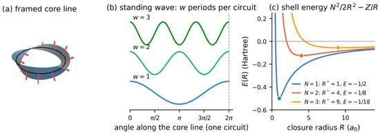
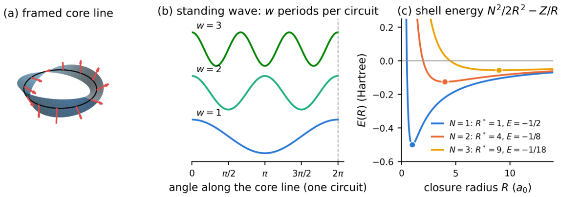
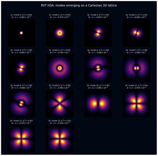
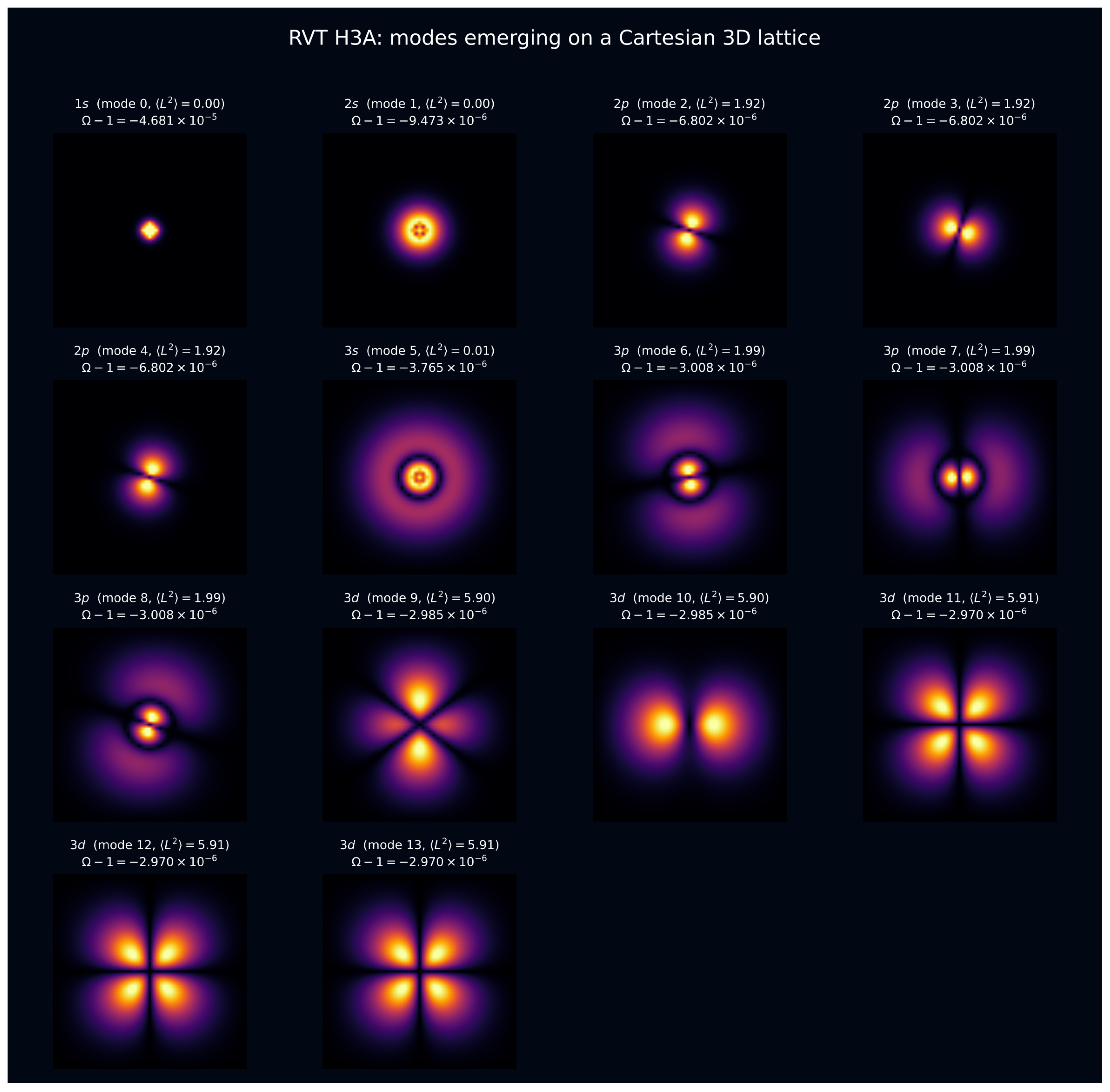
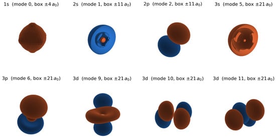
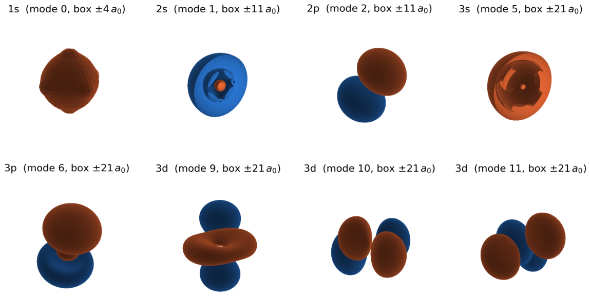
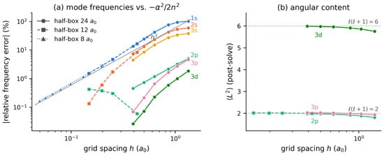
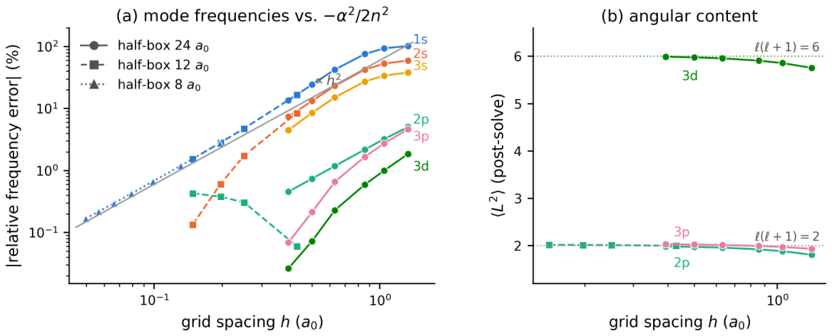
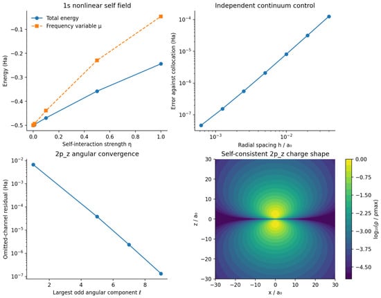
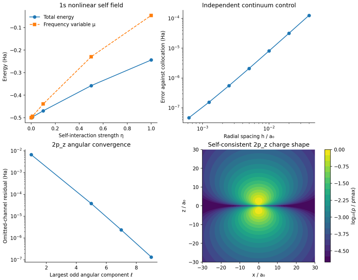

Disclaimer/Publisher’s Note: The statements, opinions and data contained in all publications are solely those of the individual author(s) and contributor(s) and not of MDPI and/or the editor(s). MDPI and/or the editor(s) disclaim responsibility for any injury to people or property resulting from any ideas, methods, instructions or products referred to in the content. |
© 2026 by the author. Licensee MDPI, Basel, Switzerland. This article is an open access article distributed under the terms and conditions of the Creative Commons Attribution (CC BY) license.