


Abstract
The booming data volume of modern time-domain surveys demands fast, robust early classification of sparsely sampled light curves, as newly discovered transients typically have only a handful of observations. We compare classifiers for extremely sparse light curves (3–30 observations) on a benchmark of approximately 1.72 million segments spanning seven astrophysical classes from ZTF and ATLAS. Methods include handcrafted-feature approaches (XGBoost, feature-based Transformers) and end-to-end LSTM and Transformer models. A pre-trained end-to-end Transformer achieves test accuracy of 0.946 (macro F1 0.950), exceeding 90% accuracy with only seven observations, but falls to 0.513 without pre-training. XGBoost-Reduced (38 features, excluding LS descriptors) reaches 0.922, while XGBoost-Full (56 features) reaches 0.913. Reliability diagnostics confirm LS periods and false-alarm probabilities are unreliable on 3–30-point segments; restricting training and evaluation to ≥15 points does not reverse the full-scale preference for the Reduced catalog. On CPU, XGBoost runtime is dominated by feature extraction (ratio ≈ 16:1); adding LS descriptors increases total processing time by ∼7.8% (feature extraction by ∼7.0%) without a commensurate accuracy gain. A lightweight LSTM attains 0.847 accuracy with 0.2 M parameters. These results offer practical guidance for model selection in real-time survey pipelines.
1. Introduction
Variable stars are ubiquitous throughout the Universe and exhibit brightness variations over timescales ranging from minutes to years. These variations originate from diverse physical mechanisms, including stellar pulsation, eclipsing binary interactions, rotational modulation, magnetic activity, and eruptive phenomena. The study of stellar variability provides fundamental insights into stellar structure, evolution, and physical properties, while many classes of variable and transient objects serve as indispensable astrophysical probes. For example, the period–luminosity relation of classical Cepheids forms the foundation of the extragalactic distance scale [1], whereas Type Ia supernovae are widely used as cosmological distance indicators for measuring the expansion history of the Universe [2]. Consequently, accurate identification and classification of variable astronomical sources constitute an essential task in modern time-domain astronomy and play an important role in both stellar astrophysics and observational cosmology.
The rapid development of wide-field time-domain surveys has fundamentally transformed astronomical observations during the past two decades. Modern facilities continuously monitor large fractions of the sky and generate enormous volumes of multi-epoch photometric data, enabling population-scale investigations that were previously impossible. Representative surveys, including the Kepler mission [3], the All-Sky Automated Survey for Supernovae (ASAS-SN; [4,5]), the Gaia survey [6], the Zwicky Transient Facility (ZTF; [7]), and the Transiting Exoplanet Survey Satellite (TESS; [8]) have collectively produced millions of high-quality light curves spanning diverse classes of variable stars and transient phenomena. The unprecedented growth of survey data has simultaneously created an urgent demand for automated classification techniques capable of processing massive alert streams. In modern survey pipelines, newly detected objects are typically represented by only a limited number of early observations, yet rapid preliminary classification is required to prioritize follow-up observations and distinguish known variable stars from genuinely new transient events. This challenge will become even more significant for the Vera C. Rubin Observatory’s Legacy Survey of Space and Time (LSST; [9]), which is expected to generate approximately ten million alerts every night, placing stringent requirements on both the accuracy and computational efficiency of automated classification methods.
Machine-learning techniques have therefore become one of the dominant approaches for astronomical light-curve classification. Conventional methods generally extract handcrafted statistical, temporal, uncertainty-related, and periodic features from light curves before applying supervised learning algorithms such as Random Forests, Support Vector Machines, or gradient boosting methods [10,11,12]. Benefiting from carefully designed feature representations, these approaches have achieved excellent performance for many variable-star classification tasks. More recently, deep-learning models capable of learning feature representations directly from sequential observations have attracted increasing attention. Recurrent and attention-based architectures have been applied to early transient classification and photometric typing [13,14,15,16], including long short-term memory (LSTM) networks [17] and Transformer-based models [18]. Nevertheless, most existing studies have focused on relatively well-sampled light curves or specific model architectures. Early classification based on extremely sparse observations remains substantially more challenging because only limited temporal information is available, many commonly used variability descriptors become unreliable, and sequence-learning models often struggle to extract representative temporal patterns from very short observation sequences. Furthermore, systematic comparisons among different learning paradigms under a shared sparse-light-curve benchmark with a common partition and evaluation protocol remain relatively scarce, particularly with respect to classification robustness, computational efficiency, feature effectiveness, and practical deployment in real-time survey pipelines.
In this work, we present a systematic benchmark comparison for the early classification of extremely sparse astronomical light curves. Rather than emphasizing a single classification algorithm, we investigate representative feature-based and sequence-based learning paradigms under a unified experimental design. This study integrates handcrafted statistical, temporal, uncertainty-related, and periodic features with gradient-boosting models, while also evaluating deep-learning approaches operating directly on raw light-curve sequences. In addition to overall classification performance, we further investigate the influence of observation number, feature contribution, computational efficiency, and model deployment characteristics to provide a comprehensive assessment of different machine-learning strategies for sparse light-curve classification. These results are intended to provide practical guidance for future real-time classification systems in large-scale time-domain surveys.
The remainder of this paper is organized as follows. Section 2 describes the datasets, sparse light-curve construction, and preprocessing procedures. Section 3 introduces the benchmark methodology, including handcrafted feature extraction, machine-learning models, deep-learning architectures, and evaluation metrics. Section 4 presents the experimental results and comparative analyses. Section 5 discusses the implications, limitations, and practical applications of the benchmark. Finally, Section 6 summarizes the conclusions of this work.
2. Data Preparation
The benchmark dataset used in this work consists of variable stars collected from the Zwicky Transient Facility (ZTF) and supernovae obtained from the Asteroid Terrestrial-impact Last Alert System (ATLAS; [19]). These two surveys provide complementary observations of periodic stellar variability and rapidly evolving transient events, enabling the construction of a unified benchmark for early light-curve classification. Instead of directly employing complete light curves, all observations are processed through a unified data preparation pipeline to generate sparse observational segments that emulate the limited information available immediately after source discovery. The following sections describe the survey data, sample selection criteria, sparse light-curve construction procedures, and dataset partition adopted throughout this work.
2.1. ZTF Light Curves
ZTF provides one of the richest publicly available optical time-domain datasets for the study of variable stars. Operating from Palomar Observatory with a 47 field of view, ZTF surveys the northern sky in three custom filters, i.e., , , and , with typical cadences ranging from hours to days [7]. Its high observing cadence and wide sky coverage have made ZTF one of the most widely used datasets for machine-learning studies of stellar variability. We adopt variability classes from the ZTF periodic variable catalog [20,21], which identified 781,602 periodic variables in ZTF DR2 using Lomb–Scargle periodograms and DBSCAN clustering, classifying them into 11 types including Scuti (DSCT), Algol-type (EA) and W Ursae Majoris-type (EW) eclipsing binaries, RR Lyrae (RR and RRc subtypes), classical (CEP) and Type II (CEPII) Cepheids, semiregular (SR) and Mira long-period variables, and rotational variables (BY Dra and RS CVn). In that taxonomy, the label RR denotes fundamental-mode (RRab-like) RR Lyrae, while RRc denotes first-overtone stars; double-mode RRd variables are not present among the catalog labels used here. Our experiments use the following subclasses before merging: BY Dra, CEP, CEPII, CV, DSCT, EA, EW, Mira, RR, RRc, RSCVN, and SR. Here CV denotes cataclysmic variables (accreting white-dwarf binaries such as dwarf novae and related outbursting systems); CV labels are taken from the extended IPAC release and lie outside that 11-type taxonomy. To simulate the sparse observational conditions relevant to real-time classification, we segment each multi-epoch light curve into shorter subsequences containing between 3 and 30 observations, which follows three criteria: (1) each subsequence must be monochromatic (i.e., confined to a single filter); (2) any gap longer than 10 days within a given band triggers a new subsequence; (3) we maximize the number of segments while ensuring a uniform distribution across observation counts (Figure 1). These criteria are designed to preserve temporal continuity while maximizing the number of usable sparse light curves for subsequent machine-learning experiments.
Figure 1.
Three segmentation criteria for sparse light-curve construction (each point denotes one photometric detection: magnitude measured at a given epoch in a ZTF filter). (a) Monochromatic segmentation by filter. (b) Gap-based segmentation within a single band, where a temporal gap exceeding 10 days initiates a new segment. (c) Sliding windows of L consecutive detections (–30) extracted from a monochromatic block; the shaded interval shows one example with .
Figure 2 shows example monochromatic parent blocks together with contiguous sparse excerpts (, 15, and 30) for an RR Lyrae and an eclipsing-binary source.
Figure 2.
Monochromatic parent blocks versus sparse segments used for early classification. (a) RR Lyrae and (b) W UMa-type eclipsing binary (EW). Left: reconstructed single-filter parent block (). Shading marks the excerpt window. Right: sparse segments with , 15, and 30 points from the same block. Connecting lines follow chronological order for visualization only.
Criteria (1)–(2) yield the following numbers of monochromatic parent blocks for each variability class: BY Dra (5880), CEP (4279), CEPII (1238), CV (8591), DSCT (2293), EA (2268), EW (11,704), Mira (3478), RR (4293), RRc (3374), RSCVN (4042), and SR (2274). Criterion (3) then extracts contiguous windows of –30 detections from these blocks, producing the large pool of sparse segments used for training and evaluation; after combination with the SN sample and partial rebalancing, the final train/validation/test sizes are reported in Section 2.3. These windows serve as segment-level training samples under an object-level split, so that multiple segments from the same source remain within a single subset rather than being treated as fully independent objects. To reduce class complexity and mitigate data imbalance, we merge related types as follows:
- RRab and RRc are combined into a single RR Lyrae class;
- EA and EW are grouped as eclipsing binaries;
- Mira and SR are merged into long-period variables (LPVs);
- BY Dra and RSCVN are unified as “active” stars;
- CEP, CEPII, and DSCT are grouped as “pulsating” variables;
- CV is retained as its own cataclysmic-variable class.
The merged ZTF variable-star classes are intentionally coarse, reflecting the goal of rapid very-early classification rather than detailed astrophysical subclassification. They are later combined with the supernova sample (Section 2.2) and rebalanced as described in Section 2.3.
2.2. Supernovae
We identify 2575 objects reported to the Transient Name Server (TNS, https://www.wis-tns.org/) between 2018 and 2025 that have publicly available forced photometry from ATLAS. Of these, 1872 are confirmed supernovae and 703 are Astronomical Transients (AT, transients reported without spectral validation, may be SNe, flare stars or artifacts). Only the confirmed-SN subset enters our SN class; the remaining 703 objects are not used. From the confirmed-SN group, we cross-match ATLAS/TNS sources with ZTF light curves to obtain multi-survey photometry anchored to the discovery epoch; however, only 413 confirmed SNe exhibit sufficiently sampled and high-quality photometric coverage in ZTF.
Anchoring all observations to the discovery Modified Julian Date (MJD), we retain only those light curves satisfying two criteria for early-phase classification: (1) observations span from at least 10 days before to 30 days after the discovery date; (2) the light curve contains at least three detections. This selection yields 146 usable ZTF light curves.
Given the limited size of this sample, we augment it by generating synthetic light curves from ATLAS data, resampled to mimic the typical cadence of ZTF. The median inter-observation interval is about 0.087 days for ZTF and about 0.003 days for ATLAS, motivating a down-sampling strategy to bridge the cadence gap.
For each ZTF light curve, we generate multiple short subsequences containing 3–30 epochs. Sampling prioritizes epochs symmetrically around the discovery date; if data exist on only one side, the nearest observation must fall within 10 days of discovery. We respect the band information and allow for repeated sampling of individual data points. When an observation includes a photometric uncertainty, we perturb its magnitude by a random draw from a Gaussian distribution with equal to the reported error; otherwise, the original magnitude is used. To avoid over-representation, no single epoch is sampled more than five times. This procedure yields 3808 ZTF-derived sparse segments.
We apply a similar resampling scheme to the ATLAS light curves but impose an additional constraint on temporal spacing: consecutive observations in each subsequence must be separated by 0.08 to 0.10 days, closely matching ZTF’s typical cadence. This results in 42,537 ATLAS-resampled sparse segments. All ZTF- and ATLAS-derived supernova light curves are merged into a single “SN” class before dataset partition, comprising 42,537 ATLAS-resampled sparse segments and 3808 ZTF-augmented sparse segments (46,345 SN segments in total) from confirmed-SN TNS/ATLAS photometry and 146 quality-selected ZTF parent light curves, respectively.
2.3. Dataset Partition
We assemble the merged ZTF variable-star segments with the SN segments of Section 2.2. Before splitting, we apply partial class rebalancing once to this combined benchmark: any ZTF variable-star class whose count exceeds four times that of the smallest ZTF class is randomly downsampled to that cap (ratio 4.0, random seed 42); SN segments are not subject to this cap. We then split the dataset into training, validation, and testing subsets at a ratio of 75:10:15. The partition is performed at the object level—rather than at the light-curve level—to ensure that all sparse samples originating from the same source remain within a single subset, thereby preventing information leakage while maintaining comparable class distributions across subsets via stratified sampling. After partial rebalancing and stratified partitioning, the final dataset contains 1,288,707 training samples, 171,828 validation samples, and 257,742 test samples.
Figure 3 summarizes the composition of the benchmark test set. The observation counts are uniformly distributed from 3 to 30 (Figure 3a), with approximately 9200 samples per count, ensuring that model evaluation is not biased toward any particular degree of sparsity. Figure 3b shows the class proportions after partial rebalancing and stratified splitting. The mean number of observations per class is nearly identical across all seven variability types (Figure 3c, –), confirming that class-wise performance comparisons are not confounded by systematic differences in sampling completeness. Test accuracy is used as the primary ranking metric in the main comparison (Section 4.1); macro F1 is also reported.
Figure 3.
Data distribution of the benchmark test set (257,742 samples). (a) Observation count distribution showing uniform coverage from 3 to 30 observations (mean ≈ 16.5). (b) Class distribution after partial rebalancing and stratified splitting. (c) Per-class observation count distribution demonstrating near-identical mean observation numbers across all seven variability types, ruling out sampling completeness as a confounding factor in class-wise performance comparisons.
3. Methods
3.1. Overall Framework
To investigate the influence of different data representations on sparse light-curve classification, we consider both handcrafted feature representations and raw sequential observations under a unified experimental design implemented in Python 3.12 with XGBoost 2.1.3, Optuna 4.8, and PyTorch 2.7.0.
The first strategy follows the conventional feature-engineering paradigm: each sparse light curve is transformed into a fixed-length feature vector through handcrafted feature extraction, which is then used as input to supervised classifiers. The second strategy preserves the original temporal structure of the observations and employs sequence-based neural networks to learn representations directly from raw light-curve data.
For the feature-based pipeline, we evaluate two classifiers: XGBoost, a gradient-boosted tree ensemble, and a Feature-based Transformer encoder. For the sequence-based pipeline, we adopt an End-to-End Transformer (E2E Transformer) and an LSTM network as representative architectures. This design compares four representative model families spanning both representation strategies; Section 4.1 additionally reports feature-ablation variants (XGBoost-Full vs. XGBoost-Reduced) and alternative training regimes (from scratch, pre-training/fine-tuning, and E2E Small).
Both pipelines are trained and evaluated using the identical 75/10/15 stratified split described in Section 2. The following subsections describe the two representation strategies, the classification models, the training protocols, and the evaluation metrics.
3.2. Light-Curve Representation
3.2.1. Handcrafted Feature Extraction
For extremely short light curves, particularly those with only 3 to 5 observations, the raw time series contains minimal information. To mitigate this sparsity and extract discriminative signal, we compute a comprehensive set of handcrafted features that robustly encode statistical, temporal, periodic, and observational properties, even in low-data regimes. Our feature design follows established light-curve characterization practice [10,12] and is guided by the need to capture diverse aspects of photometric behavior while remaining resilient to irregular sampling, heteroscedastic uncertainties, and extreme data sparsity typical of modern surveys such as ZTF [7,22]. The handcrafted feature catalog used by the main models comprises 56 descriptors (grouped into ten categories in Table 1). Definitions of the less self-explanatory descriptors are collected in Appendix B. All main results in Table 2 use this catalog (or the 38-feature subset without Lomb–Scargle columns). Appendix C.1 reports a controlled check that adds ndethist to the otherwise identical Reduced catalog.
Table 1.
The 56 handcrafted features used by the main models in this study, grouped by category. Bold font denotes the summary row.
The Lomb–Scargle periodogram [23] is computed for each sparse segment independently (3–30 epochs per segment, not from the parent multi-epoch light curve), with a period grid adaptively determined by the time baseline and sampling pattern of that segment. From the periodogram, we extract 10 numerical descriptors (Table 1), the binary flag is_periodic (peak FAP threshold 0.01), and seven missing-value indicators for descriptors that cannot be computed from too few epochs. These 18 columns are present only in the 56-feature catalog; the 38-feature subset used by XGBoost-Reduced omits them (Section 3.3.1). The Stetson J variability index [24] is included among the error-aware statistics.
Observational Metadata (band_code)
The main feature catalog includes a single observational metadata column, band_code, which encodes the photometric filter for ZTF variable-star segments (1 for , 2 for , 3 for , 4 for other bands). For SN segments, band_code is sampled from the empirical ZTF variable-star band distribution with a deterministic seed derived from the segment file path. In ZTF alert packets, ndethist denotes the number of spatially coincident difference-image detections at a source position since the start of the survey [7,25]. Because our sparse segment files contain only mjd and mag, parent-level ndethist is unavailable; a fallback that sets ndethist to the segment length for ZTF variables and to zero for ATLAS SN segments correlates strongly with class and survey membership. The main models therefore omit ndethist. Appendix C.1 evaluates a variant that retains this column under the same SN band_code sampling.
Missing Value Handling
Missing values arise when a descriptor cannot be computed from the available epochs. Segments with fewer than three points are discarded at feature extraction. For the 56-feature set, we retain the missingness pattern with seven binary *_is_missing indicators (Table 1), following the missing-indicator method commonly used with constant imputation when missingness itself is informative [26]. Uncomputable numerical entries are set to 0.0 (zero imputation) rather than a training-set mean or median, so that no distributional prior estimated from other objects is injected into the feature values. In the 38-feature baseline set, missing-indicator columns are removed; descriptors that remain undefined for the retained sampling (e.g., kurtosis when ) are likewise set to 0.0, while num_points remains available for the classifier to assess reliability. Zero fill is a practical requirement for feature standardization and tree-based training; combined with missing indicators (56-feature set) or observation count (38-feature set), it preserves sparsity information without median-based prior leakage.
Feature Standardization
All non-binary features are standardized as
where and are the training-set mean and standard deviation of feature i. The same and are applied to the validation and test sets to prevent data leakage. Binary features, including missing-value indicators and is_periodic, are left unstandardized. The standardized feature vectors serve as inputs to the XGBoost classifier.
3.2.2. Raw Sequence Representation
Unlike the feature-based representation, sequence-based models operate directly on the original sparse observations without handcrafted feature extraction. Each sparse light curve is represented as an ordered sequence of photometric measurements that preserves the temporal ordering of the observations.
Each observation is represented by a triplet
where denotes the elapsed time since the first observation of the light curve (i.e., ), is the calibrated magnitude, and is the corresponding photometric band identifier. Since each sparse light-curve segment is constructed within a single photometric filter, the band identifier remains constant throughout an individual sequence.
A sparse light curve containing L observations () is therefore represented as
This representation preserves both the chronological ordering of the observations and the associated photometric-band information, enabling sequential neural networks to learn temporal characteristics directly from the observational data without manually designed statistical descriptors.
Since different light curves contain different numbers of observations, variable-length sequences are retained throughout data preparation. During model training, sequences within each mini-batch are padded to the maximum sequence length of that batch, while the corresponding padding masks ensure that padded positions do not contribute to model computation. This dynamic padding strategy improves computational efficiency while preserving the original temporal structure of individual light curves.
3.3. Classification Models
To comprehensively evaluate different learning paradigms for early classification of sparse astronomical light curves, we investigate four representative model families: XGBoost and a Feature-based Transformer on handcrafted features, and an LSTM and an E2E Transformer on raw sequences. All models are trained and evaluated using the same benchmark dataset, data partition, and evaluation metrics.
3.3.1. XGBoost
XGBoost (Extreme Gradient Boosting) [27] is a supervised ensemble-learning algorithm based on gradient-boosted decision trees and has become one of the most successful machine-learning approaches for structured tabular data. By combining second-order gradient optimization, regularization, and efficient parallel tree construction, XGBoost achieves high predictive accuracy while maintaining relatively low computational cost and strong generalization capability. Owing to these advantages, XGBoost has been widely applied to astronomical classification problems involving heterogeneous feature sets.
In this work, XGBoost is the primary feature-based classifier. We evaluate two input catalogs (Section 3.2.1): XGBoost-Reduced(38 features; no LS columns) as the baseline for main comparisons, and XGBoost-Full (56 features) as a control that adds the 18 Lomb–Scargle-related columns to that baseline. Handcrafted feature vectors are used directly as inputs; tree ensembles are well suited to these heterogeneous, sparsely sampled descriptors.
Rather than manually selecting model hyperparameters, we employ Optuna [28] to automatically optimize the XGBoost configuration using Bayesian hyperparameter optimization. The search space includes the learning rate, maximum tree depth, number of estimators, subsampling ratio, column sampling ratio, minimum child weight, gamma, and regularization parameters. Optuna maximizes three-fold stratified cross-validation accuracy on the training split. Model rankings in the main text are based on test-set accuracy. Following hyperparameter optimization, the final XGBoost classifiers are retrained using the optimized parameter sets and subsequently evaluated on the independent test dataset.
3.3.2. LSTM
To provide a representative recurrent neural-network baseline for sequence-based learning, we employ a two-layer LSTM network [17] (hidden dimension 128, dropout 0.2) to classify sparse light curves directly from the original observational sequences. Unlike feature-based methods, the LSTM does not rely on handcrafted descriptors but instead learns temporal representations from sequential photometric measurements through recurrent memory units.
The input to the network follows the raw sequence representation. Each observation is represented by a three-dimensional vector containing the relative observation time, calibrated magnitude, and photometric band identifier. The LSTM sequentially processes the observations in chronological order while maintaining an internal memory state that summarizes previously observed temporal information. At each time step, the hidden state is updated through three gating mechanisms controlling information propagation. After the final observation has been processed, the last hidden state is fed into a fully connected classification layer followed by a softmax activation to produce the probability distribution over all variability classes.
Since sparse light curves contain only a limited number of observations, variable-length sequences are handled using the padding and masking strategy. Masked positions do not contribute to either hidden-state updates or loss computation, ensuring that sequence lengths do not introduce systematic biases during training. The LSTM serves in this work as a representative sequence-learning baseline against which the Transformer-based models can be systematically compared.
3.3.3. Transformer Models
Transformer is a deep neural network architecture based on the self-attention mechanism, which enables each element in the input sequence to directly interact with every other element without relying on recurrent computations. Compared with recurrent neural networks, Transformer models are capable of capturing long-range dependencies through global attention while allowing efficient parallel computation during training.
In this work, Transformer models are investigated under two complementary data representations:
- Feature-based Transformer: operates on the 56-dimensional handcrafted feature vector for each sparse segment (same inputs as XGBoost-Full). Each feature vector is linearly projected to the model dimension, treated as a length-1 token sequence, processed by the Transformer encoder, and summarized by mean pooling before a classification head (rather than treating each scalar feature as a separate token). This model is evaluated both from scratch and with fine-tuning from a 50-observation pre-trained checkpoint (Table 2).
- End-to-End Transformer (E2E Transformer): directly learns temporal representations from the original observational sequences (time, magnitude, band). Each observation is projected into the embedding space, positional encodings are added to preserve temporal ordering, and a dynamic padding strategy handles variable-length sequences. The model employs a two-stage training strategy: supervised pre-training on light curves with exactly 50 observations (fixed length), followed by fine-tuning on sparse light curves with 3 to 30 observations (variable length). The full E2E Transformer uses the same 18-layer encoder configuration as the feature-based variant (Table 2; architecture details in Table A3). A lightweight E2E Transformer Small variant (10.2 M parameters) is also evaluated.
The feature-based and full E2E Transformers are configured at comparable model capacity to isolate the effect of input representation; they differ only in whether the input is a handcrafted feature vector or a raw photometric sequence.
3.4. Model Training
To ensure a fair comparison among different learning paradigms, all classifiers are trained using the identical training, validation, and testing partitions. Hyperparameter optimization, model selection, and early stopping are performed exclusively in the validation set, while the independent test set is reserved for the final performance evaluation. This unified experimental protocol minimizes potential evaluation bias and enables an objective comparison between feature-based and sequence-based classification methods.
The hyperparameters of the XGBoost classifiers are optimized using the Optuna framework, which performs efficient Bayesian optimization. For the deep-learning models, hyperparameters are selected empirically based on validation performance and remain fixed throughout all experiments. The principal hyperparameters include the embedding dimension, number of Transformer encoder layers, number of attention heads, hidden dimension of the feed-forward network, dropout rate, batch size, learning rate, and weight decay.
For the Transformer models, a two-stage optimization strategy is employed. During the pre-training stage, the model is trained on light curves with a fixed length of exactly 50 observations. After pre-training, the learned model parameters are transferred to the target dataset and fine-tuned using sparse light curves containing only 3–30 observations. To prevent information leakage, the pre-training and fine-tuning datasets are constructed using independent object-level partitions. For comparison, all Transformer models are additionally trained from random initialization without pre-training.
3.5. Evaluation Protocol
To comprehensively evaluate different machine-learning approaches for sparse light-curve classification, we assess all models from multiple perspectives, including classification performance, robustness under different observation numbers, feature contribution, computational efficiency, and training strategy.
3.5.1. Classification Metrics
For multi-class classification, overall accuracy is defined as the ratio of correctly classified samples to the total number of test samples. We use test accuracy as the primary metric for model ranking and comparison throughout this work, including the per-observation-count analyses in Section 4.4. XGBoost hyperparameters are optimized separately with Optuna to maximize three-fold stratified cross-validation accuracy on the training split. We also report macro F1, precision, and recall, and present confusion matrices for class-wise behavior.
3.5.2. Observation-Number Evaluation
Since the primary objective of this work is the early classification of extremely sparse light curves, model performance is further evaluated as a function of the number of available observations. The testing dataset is divided according to the number of observations contained in each sparse light curve, ranging from 3 to 30 epochs. Classification accuracy is calculated independently for each subset. This evaluation quantitatively measures how rapidly different models become reliable as additional observations are accumulated.
3.5.3. Feature Contribution Analysis
For feature-based models, the contribution of handcrafted descriptors is investigated through XGBoost feature-importance scores and feature-ablation experiments. Feature-ablation experiments, conducted on a 50,000-sample random training subset with fixed hyperparameters to isolate per-feature-group contributions, are presented in Appendix C.
3.5.4. Computational Efficiency Evaluation
Besides classification accuracy, computational efficiency is an important consideration for real-time astronomical surveys. Different observational facilities possess substantially different computing resources, ranging from GPU-equipped data centers to CPU-only observatories and local processing systems. Therefore, computational efficiency is evaluated under both GPU and CPU environments. For each model, we record the training time, feature extraction time (if applicable), inference latency, model size, and GPU memory consumption.
4. Results
4.1. Overall Classification Performance
Table 2 presents the overall classification performance of all evaluated models on the independent test set containing 257,742 sparse light curves (3–30 observations).
Table 2.
Overall classification performance of all models on the sparse light-curve test set (257,742 samples, 3–30 observations). Models are ranked by test accuracy. Trainable parameter counts (M) are reported for neural networks; on-disk serialized model file size (MB) is reported for XGBoost models. Bold values indicate the highest test accuracy and the smallest trainable parameter count.
The pre-trained E2E Transformer leads the ranking (accuracy 0.946; macro F1 0.950), whereas the same architecture without pre-training falls to 0.513—a ∼43 percentage-point gap that underscores the role of transfer learning. Among feature-based models, XGBoost-Reduced (0.922) outperforms XGBoost-Full (0.913); the LS comparison is developed in Section 4.2.2. The LSTM reaches 0.847 with only 0.2 M parameters, remaining below XGBoost-Reduced on CPU (Section 5.4). On the same 56 handcrafted features, the Feature-based Transformer (0.878 from scratch; 0.823 fine-tuned) underperforms XGBoost, consistent with tree ensembles on heterogeneous tabular inputs [29] and with negative transfer from 50-observation pre-training features to the 3–30-epoch regime.
Figure 4 shows confusion matrices for four representative models. SN recall is near ceiling for XGBoost-Reduced and the pre-trained E2E Transformer (Figure 4a–c; Section 2.2 for construction caveats); the main residual confusion is among Active stars, Cataclysmic Variables, and Pulsating variables. Figure 4d (E2E without pre-training) exhibits severe cross-class errors among non-SN classes, consistent with its low overall accuracy.
Figure 4.
Confusion matrices for XGBoost-Reduced, the pre-trained E2E Transformer, the LSTM, and the E2E Transformer without pre-training on the sparse light-curve test set (3–30 observations). Values represent row-normalized recall fractions.
4.2. Analysis of Feature-Based Learning
4.2.1. Feature Importance
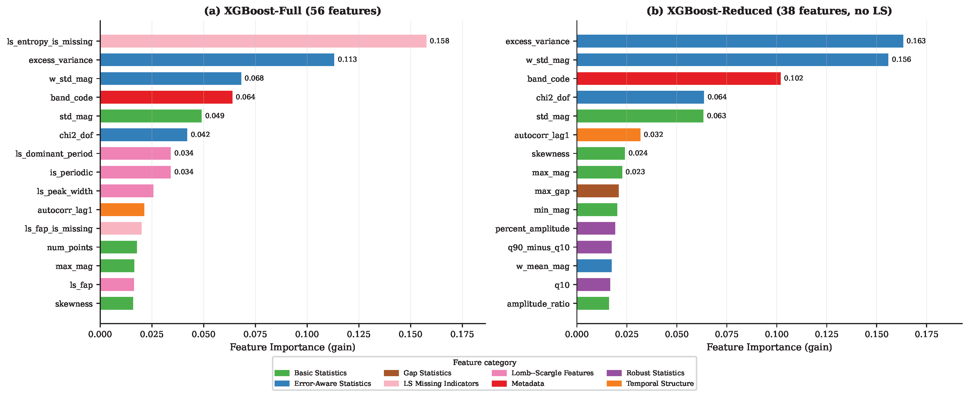
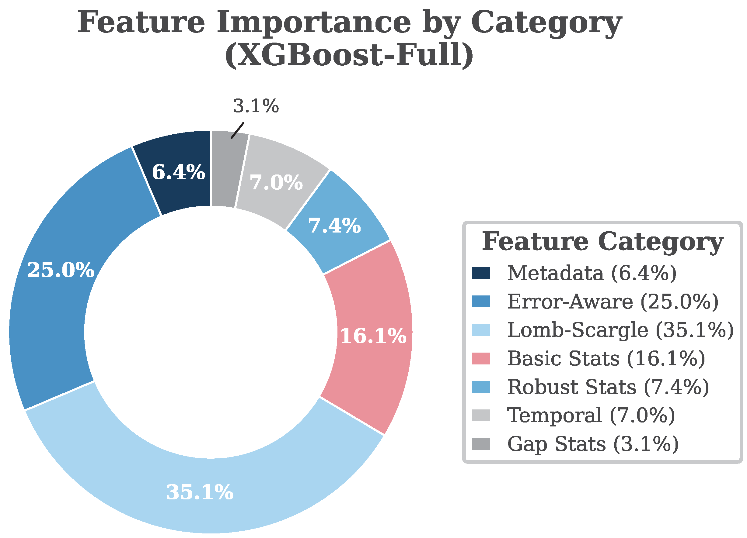
Figure 5 shows the top 15 importances from XGBoost-Full. The leading column is ls_entropy_is_missing (0.158)—a missingness indicator rather than a periodogram amplitude—followed by excess_variance (0.113), w_std_mag (0.068), and band_code (0.064). Impurity rankings can emphasize missingness flags that correlate with sparsity [30,31]; among photometric descriptors, variability-amplitude statistics dominate. The 18 Full-only columns account for 35.1% of total importance, yet removing them improves full-scale accuracy (Section 4.2.2), so importance should not be read as a net gain from sparse period estimates. Appendix C Figure A2 compares Full and Reduced rankings.
Figure 5.
Top 15 XGBoost feature importances from XGBoost-Full (56 features; Table 1), colored by feature category. ls_entropy_is_missing ranks highest; variability and error-aware statistics dominate among photometric descriptors. The 18 columns present only in XGBoost-Full account for 35.1% of total importance.
4.2.2. The Impact of Periodicity Features on Full-Scale Performance
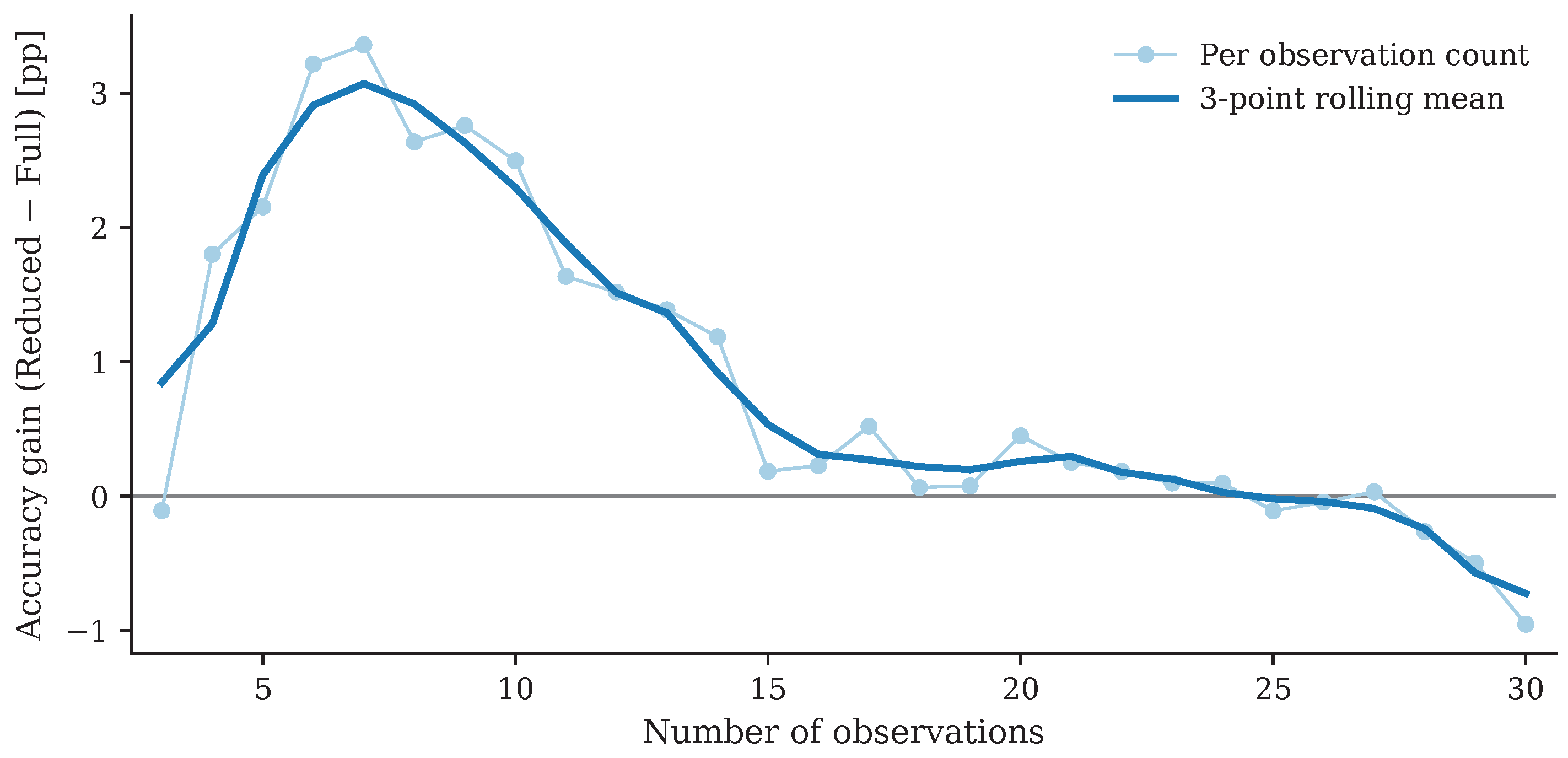
On the full-scale Optuna-tuned benchmark, XGBoost-Reduced outperforms XGBoost-Full by about 0.9 percentage points (0.922 vs. 0.913; macro F1 0.931 vs. 0.923). Figure 6a and Appendix C Figure A4 show that this advantage is concentrated at low observation counts (∼2.2 percentage points at 3–8 observations) and fades by 23–30 observations. (A 50 K fixed-hyperparameter group ablation in Appendix C can rank feature blocks differently and is not interchangeable with this full-scale comparison.)
Figure 6.
Observation count analysis. (a) XGBoost-Reduced versus XGBoost-Full across observation counts (3–30 epochs). (b) Three representative models: the pre-trained E2E Transformer surpasses 90% accuracy at 7 observations and exceeds 99% at 11 observations (annotated); XGBoost-Reduced outperforms the E2E Transformer at 3–4 observations (annotated); LSTM improves steadily. Horizontal dashed lines mark the 90% and 99% reference levels. Per-count Reduced−Full differences are quantified in Appendix C Figure A4.
Figure 7 shows that period recovery is near zero at 3–4 points and that FAP-based flags can be spuriously optimistic near five points. Even restricting training and evaluation to ≥15 observations does not establish a robust Full advantage under the same Optuna hyperparameters (Reduced remains slightly higher by 0.05 percentage points). These results are consistent with the need for adequate phase coverage in periodogram analysis [23] and support the 38-feature baseline as the default feature-based configuration in the 3–30-epoch regime.
Figure 7.
Reliability of Lomb–Scargle summaries on sparse segments (periodic variable-star test segments; SN excluded). (a) Median relative period error versus a longer-segment reference. (b) Fraction of segments with period agreement within 10% and 50%. (c) Fractions with FAP and is_periodic = 1. At low observation counts, periods are poorly recovered while FAP-based flags can be spuriously optimistic.
4.3. Analysis of Sequence-Based Learning
4.3.1. Raw Sequence vs. Feature Input
The comparison between Transformer models using raw sequences vs. handcrafted features (Table 2) reveals that input representation fundamentally determines model capability. The pre-trained E2E Transformer achieves the best overall performance, demonstrating that—with adequate pre-training—deep architectures can learn effective representations directly from sparse photometric sequences. For the handcrafted-feature pipeline (56 dimensions), XGBoost outperforms both Feature-based Transformer variants; tree-based ensembles remain more effective than attention-based architectures on heterogeneous tabular inputs [29]. Fine-tuning the Feature-based Transformer degrades performance relative to training from scratch (Δaccuracy = −0.055), indicating negative transfer when the 50-observation pre-training feature distribution differs from the 3–30 observation target regime, especially for LS-derived quantities. Self-attention is more effective on raw temporal sequences than on pre-compressed descriptors because raw inputs preserve ordering and inter-observation relationships [18].
4.3.2. Effect of Transformer Pre-Training
Figure 8 illustrates the impact of pre-training on Transformer classification performance. For the E2E Transformer, pre-training on 50-observation light curves improves test accuracy from 0.513 to 0.946 (macro F1 from 0.552 to 0.950), a gain of 0.433 in accuracy, yielding the best-performing model in our comparison. The near-perfect pre-training performance (test accuracy ≈ 0.999 on the independent 50-observation test set) should not be interpreted as performance on the early sparse task. It reflects supervised classification on relatively well-sampled, fixed-length (50-epoch) light curves drawn from a separate 50obs data pool, after the same seven-class merging scheme, where class-discriminative variability patterns (period, amplitude, morphology) are substantially more complete than in 3–30-observation segments. The pre-training objects and the 3–30 fine-tuning/test objects are object-disjoint under our 75/10/15 split; they are not different segments sampled from the same parent light curve. The relevant operational result is therefore the fine-tuned performance on the independent 3–30 observation test set (accuracy = 0.946; macro F1 = 0.950; Table 2). During pre-training, the Transformer encoder learns general temporal representations from these relatively complete patterns; when transferred to the sparse regime, these pre-trained representations provide a strong inductive bias that enables the model to extract meaningful features even from very few data points.
Figure 8.
Effect of pre-training on Transformer classification performance (test accuracy). The E2E Transformer improves substantially with pre-training (Δaccuracy = +0.433), while the Feature-based Transformer shows negative transfer (Δaccuracy = −0.055).
For the Feature-based Transformer, the negative transfer effect (fine-tuned worse than from scratch) likely occurs because the pre-trained model learns to attend to feature interactions that are informative for 50-observation light curves but become misleading for 3–30 observation data, where feature distributions—particularly those of LS-derived quantities—shift substantially.
4.4. Robustness Under Sparse Observations
Figure 6b presents the classification accuracy of three representative models as a function of the number of available observations. Several key observations emerge:
- Rapid convergence of pre-trained E2E Transformer: The E2E Transformer with pre-training surpasses 90% accuracy at only 7 observations and exceeds 99% at 11 observations. This rapid convergence is a direct consequence of the pre-trained representations that enable efficient extraction of temporal features from minimal data.
- XGBoost advantage at very few observations: Notably, XGBoost-Reduced outperforms the pre-trained E2E Transformer at three to four observations, where handcrafted statistical descriptors remain informative while sequence-based models have insufficient temporal context. From five observations onward, the E2E Transformer takes the lead.
- Steady LSTM improvement: The LSTM exhibits a gradual, nearly linear improvement with observation count, reflecting the gating mechanisms that provide inherent robustness to short sequences. Unlike the Transformer, it shows no sharp performance cliff at low observation counts.
- Pre-training as a necessity: The E2E Transformer without pre-training barely exceeds 70% accuracy even at 30 observations, performing worse than all other methods at every observation count.
- Diminishing returns beyond ∼20 observations: All models show reduced marginal gains after approximately 20 observations, indicating that the most critical classification information is contained in the first 15–20 observations.
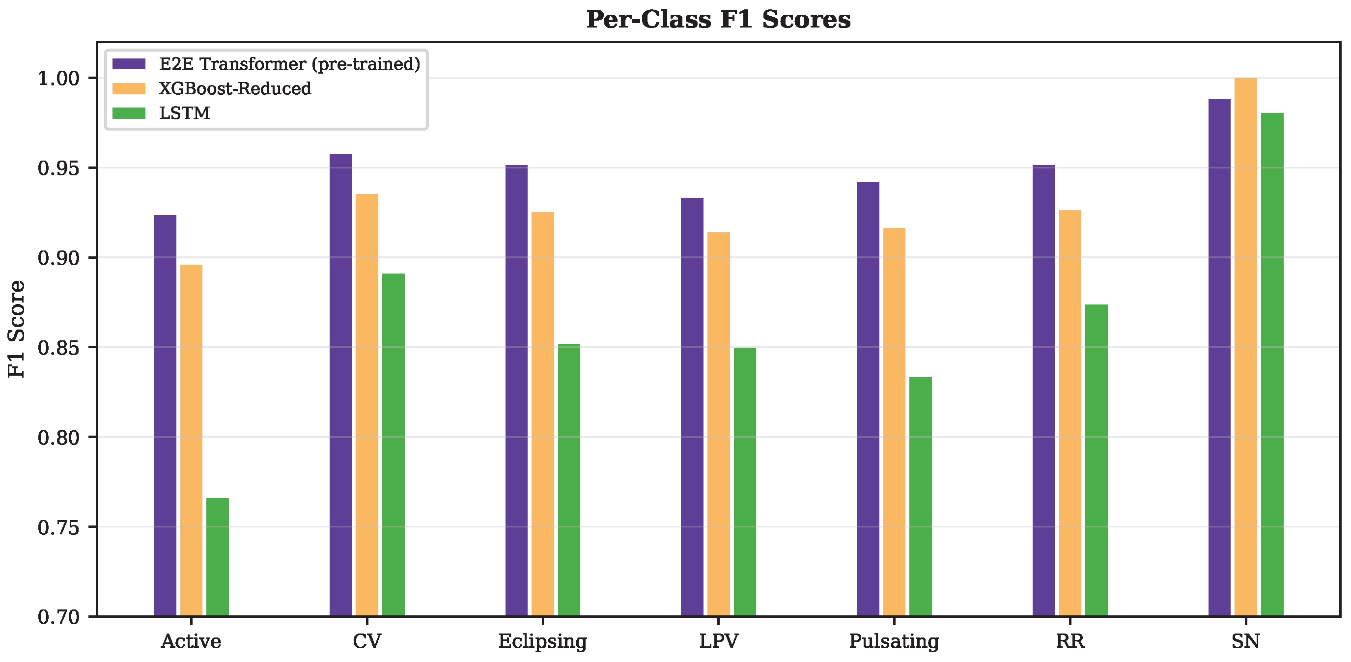
Per-class F1 scores (Appendix D Figure A7) show SN F1 ≥ 0.98 for the three representative architectures; given the resampled SN construction (Section 2.2), these scores characterize separability on the present benchmark rather than guaranteed field performance. The lowest scores are for Active stars and Pulsating variables, where sparse morphology alone is often insufficient [32,33]. Observation-count curves for the remaining models are given in Appendix G Figure A10.
4.5. Computational Efficiency
Beyond classification accuracy, computational efficiency is critical for real-time astronomical survey pipelines. All timing benchmarks were obtained on a Paratera AI Computing Cloud instance with an NVIDIA RTX 4090 GPU (NVIDIA Corporation, Santa Clara, CA, USA; 24 GB VRAM), 10 vCPUs, and 60 GB RAM: PyTorch 2.7.0-based deep-learning models were evaluated on GPU, whereas XGBoost feature extraction and inference were run on CPU. Figure 9 presents the results; complete CPU/GPU benchmark tables and supplementary plots are given in Appendix D.
Figure 9.
Computational efficiency on the full test set ( samples) under the production mixed CPU/GPU deployment setup (Table A9): XGBoost uses CPU for feature extraction and inference; end-to-end neural models use GPU inference; the feature-based Transformer uses CPU feature extraction and GPU inference. Device labels on the vertical axis indicate the hardware used for model inference. (a) Processing time breakdown (feature extraction + model inference) normalized to per 10 k samples. (b) End-to-end throughput in samples per second.
Key findings from the computational analysis:
- XGBoost dominates CPU deployment: With a total processing time of approximately 891 s for 257,742 samples on CPU, XGBoost-Reduced processes approximately 289 samples per second. Its model size (408 MB) is moderate, and it requires no GPU, making it the most practical choice for CPU-only observatories.
- LSTM is the most compact deep-learning model: At 0.77 MB and 0.2 M parameters, the LSTM is orders of magnitude smaller than XGBoost or the E2E Transformer (Figure 10). On GPU it reaches ∼14,700 samples/s (17.5 s for the full test set), the highest deep-learning inference throughput in our benchmarks.Figure 10. Model size vs. classification performance (test accuracy). The LSTM combines moderate accuracy (0.847) with extremely compact model size (0.77 MB).
- E2E Transformer requires GPU but delivers top accuracy: The pre-trained E2E Transformer processes approximately 3500 samples per second on GPU, with a model size of 868 MB. While its computational requirements are highest among the evaluated methods, its classification accuracy justifies the cost for facilities with GPU infrastructure.
- Feature extraction is the bottleneck: For feature-based XGBoost on CPU, feature extraction dominates total processing time (Figure 9; Table A8)—for example, XGBoost-Reduced requires 839.8 s for feature extraction versus 51.4 s for inference, a ratio of approximately 16:1. Adding Lomb–Scargle-related features increases feature extraction time by 58.4 s (+7.0%, from 839.8 to 898.2 s) and total processing time by 69.4 s (+7.8%, from 891.2 to 960.6 s). These timings apply only to the XGBoost pipeline; sequence-based E2E models bypass feature extraction entirely. Although Lomb–Scargle periodogram computation is the most expensive individual feature category among the descriptors evaluated, the modest wall-clock gain from removing LS features reflects the fact that non-LS descriptors and shared pipeline overhead still dominate at survey scale. Combined with the accuracy comparison in Section 4.2.2, this supports omitting LS features by default in the 3–30-epoch window; whether they become useful beyond ∼30–50 observations remains open (Section 5.5).
- CPU vs. GPU trade-off: Deep-learning models benefit from GPU acceleration (10–250× speedup; Figure A5), whereas GPU offloading provides no speedup for the XGBoost pipeline evaluated here (CPU-bound feature extraction and inference). For resource-limited environments, the LSTM achieves competitive accuracy with minimal hardware requirements.
4.6. Model Size vs. Performance
Figure 10 summarizes the size–accuracy trade-off: the LSTM is the most compact (0.77 MB at accuracy 0.847), the pre-trained E2E Transformer is largest and most accurate (868 MB; 0.946), and XGBoost-Reduced occupies an intermediate point (408 MB; 0.922).
4.7. Training Strategy and Convergence
Training wall-clock times range from 1.7 h (LSTM, 100 epochs) to 76 h (E2E Transformer pre-training on 50-observation data). The Feature-based Transformer requires 12.5 h from scratch or 8.0 h for fine-tuning after 50-observation pre-training; XGBoost Optuna tuning requires 27–46 h depending on variant (Full vs. Reduced). Epoch-level timings for all models are shown in Appendix D Figure A6.
5. Discussion
5.1. Handcrafted Features vs. Deep Representations
Model choice depends mainly on pre-training availability and deployment hardware. With longer light curves for pre-training, the E2E Transformer is the most accurate option; without them, XGBoost-Reduced remains preferable to a from-scratch E2E Transformer because handcrafted descriptors stay informative under extreme sparsity and tree ensembles handle heterogeneous tabular inputs well. High SN scores on this benchmark should be read together with the SN construction caveats in Section 2.2 and Appendix C.1; photometric variability descriptors such as w_std_mag and excess_variance remain the strongest morphology-driven contributors.
5.2. The Practical Limitations of Periodicity Features Under Extreme Sparsity
LS periodograms remain central to variability characterization on well-sampled light curves [20]. Here they are computed only from 3–30-epoch segments, where Section 4.2.2 shows that Full-only importance does not translate into a robust accuracy gain. Accordingly, we treat XGBoost-Reduced as the default feature-based configuration and XGBoost-Full as a control rather than a deployment recommendation.
5.3. Transfer Learning for Sparse Light-Curve Classification
Transfer learning strongly improves the E2E Transformer but can harm the Feature-based variant when pre-training and target distributions diverge (Figure 8). This aligns with the broader success of pre-training in deep learning [16] and extends it to irregularly sampled, extremely short photometric sequences. The strategy employed here—supervised classification on longer light curves followed by fine-tuning on sparse data—is particularly valuable because long light curves are abundant in archival survey data, while early sparse observations define the operational regime of alert brokers. For handcrafted features, negative transfer underscores the need to match feature reliability to observation count (Section 4.2.2).
5.4. Practical Implications for Time-Domain Surveys
The deployment recommendations emerging from this work depend on the available computational infrastructure:
- GPU-equipped data centers (e.g., LSST alert brokers; [25]): The pre-trained E2E Transformer is recommended for maximum accuracy. Its GPU throughput of ∼3500 samples/s can support broker-scale batch reclassification, although peak alert rates will still require parallel workers and staged filtering pipelines.
- CPU-only observatories: XGBoost-Reduced (38 features, no LS) provides the best accuracy-to-cost ratio for early classification in the 3–30-epoch regime. At 289 samples/s on CPU, it can handle moderate-scale surveys, and its Optuna tuning wall time (27–46 h, depending on variant) is manageable for periodic model updates. The LS-inclusive 56-feature catalog is not recommended as the default CPU configuration in this sparse setting (Section 5.2).
- Edge deployment: The LSTM offers a compact model (0.77 MB) with competitive but lower test accuracy (0.847; macro F1 = 0.864) than XGBoost-Reduced on CPU. It is best suited to memory-constrained nodes with GPU inference (∼14,700 samples/s); it is not recommended over XGBoost-Reduced for CPU-only, accuracy-first pipelines (item 2 above).
- Hybrid strategies: A practical pipeline could employ XGBoost-Reduced for initial classification upon alert generation and re-classify with the pre-trained E2E Transformer once about 7–11 observations have been accumulated, matching the regime where that model exceeds 90% and approaches 99% accuracy (Section 4.4). Adding LS periodogram features to the XGBoost input within the 3–30-epoch window is not recommended as a default step.
5.5. Limitations and Future Work
Several limitations of the present work should be acknowledged. First, the benchmark dataset uses observations from two optical surveys (ZTF and ATLAS), and validation on other datasets (e.g., Gaia, Kepler) would further assess generalization. We also did not include direct head-to-head comparisons with other published sparse-classification architectures such as those of [15,16]. Second, as detailed in Section 2.2, most SN training examples are resampled or synthetically augmented rather than independent, spectroscopically confirmed multi-survey events; reported SN performance should therefore be interpreted cautiously with respect to field-to-field systematics and cadence mismatch between ATLAS and ZTF. Third, by design, all supernova subclasses are merged into a single “SN” label to emphasize early transient identification rather than photometric typing; extending the benchmark to hierarchical or subtype classification is an important future direction. Fourth, fallback ndethist values written during feature extraction are not true alert-packet metadata (Section 3.2.1; Appendix C.1). Fifth, whether LS features become beneficial beyond ∼30–50 observations remains open. Sixth, object-level splits prevent cross-subset leakage, but multiple segments from the same source may coexist within a split, so metrics may be mildly optimistic relative to single-segment-per-source evaluation.
Self-supervised pre-training, multi-band or contextual inputs, and SN evaluation on independent single-survey holdouts are natural next steps. Lightweight hybrids of handcrafted features and neural representations also remain promising.
6. Conclusions
This work has presented a systematic benchmark comparison for the early classification of variable stars and supernovae from extremely sparse light curves (3–30 observations). Through comparison of feature-based methods (XGBoost, Feature-based Transformer) and sequence-based architectures (LSTM, E2E Transformer) under a shared partition and evaluation protocol—while acknowledging that SN segments follow a different construction path from ZTF variable-star slices (Section 2.2)—we arrive at the following principal conclusions:
- End-to-end Transformer with transfer learning achieves the highest accuracy in our benchmark (test accuracy = 0.946; macro F1 = 0.950). Pre-training on longer light curves is essential; without it, the same architecture remains far below practical performance (0.513 test accuracy). The pre-trained model exceeds 90% and 99% accuracy at 7 and 11 observations, respectively.
- XGBoost-Reduced is the preferred feature-based baseline (accuracy = 0.922; macro F1 = 0.931), outperforming XGBoost-Full and all deep models except the pre-trained E2E Transformer, and remaining strongest at three to four observations. Lomb–Scargle columns are not recommended as default inputs in the 3–30-epoch regime (Section 4.2.2).
- Transfer learning is a double-edged sword for Transformer models: pre-training is essential for the E2E Transformer, whereas the Feature-based variant shows negative transfer under distribution shift between 50-observation pre-training and 3–30 observation fine-tuning.
- LSTM networks offer the best accuracy-to-size ratio, achieving test accuracy of 0.847 with a 0.77 MB model file.
- Classification accuracy improves rapidly up to ∼15–20 observations, after which additional data provide diminishing returns—validating the feasibility of early classification in real-time survey pipelines.
- Feature extraction, not model inference, is the primary CPU bottleneck for feature-based methods (Section 4.5). In the 3–30-epoch window, omitting LS features is therefore the default both for accuracy and for a modest CPU saving; whether LS inputs help beyond ∼30–50 observations remains open.
The systematic comparison presented here provides practical guidance for selecting appropriate machine-learning methods for real-time astronomical classification under different observational and computational scenarios. The benchmark pipeline is survey-agnostic in design and can be adapted to future time-domain facilities, including the Vera C. Rubin Observatory’s Legacy Survey of Space and Time.
Author Contributions
Conceptualization, C.W.; methodology, C.W., X.L. and Z.Q.; software, X.L. and Z.Q.; validation, X.L.; formal analysis, X.L. and Z.Q.; investigation, X.L.; resources, C.W. and Y.L.; data curation, C.W., X.L., Z.Q. and Y.L.; writing—original draft preparation, X.L. and Z.Q.; writing—review and editing, C.W. and X.L.; visualization, X.L.; supervision, C.W. and Y.L.; project administration, C.W.; funding acquisition, C.W. and Y.L. All authors have read and agreed to the published version of the manuscript.
Funding
The support came from the Science and Education Integration Funding of University of Chinese Academy of Sciences. We also received backing from the Strategic Priority Program of the Chinese Academy of Sciences, granted under XDB41000000, XDB0550000, XDB0550100 and XDB0550102. The research is also supported by the National Astronomical Observatories, Chinese Academy of Sciences No. E4TG2001.
Data Availability Statement
The data, model training codes in this study are openly available in GitHub at https://github.com/Yu-Yang-Li/StarWhisper/tree/main, accessed on 31 August 2026.
Acknowledgments
We are grateful to the National Astronomical Observatories, Chinese Academy of Sciences, for the support from the Tianji Experimental Class Program. During the preparation of this manuscript, the authors used DeepSeek-V4-Pro, Qwen3.8-Max, GPT-5.5, and Kimi-2.6 for language polishing, improving the organization and structure of the manuscript, formatting references, and assisting with parts of the code writing. The AI-assisted code was manually checked and verified by the authors. The authors reviewed and edited all AI-assisted outputs and take full responsibility for the content of this publication.
Conflicts of Interest
The authors declare no conflicts of interest.
Abbreviations
The following abbreviations are used in this manuscript:
| ZTF | Zwicky Transient Facility |
| ATLAS | Asteroid Terrestrial-impact Last Alert System |
| LS | Lomb–Scargle |
| LSTM | Long Short-Term Memory |
| E2E Transformer | End-to-End Transformer |
| SN | Supernova |
| LPV | Long-Period Variable |
| CV | Cataclysmic Variable |
| LSST | Legacy Survey of Space and Time |
Appendix A. Hyperparameters and Training Settings
This appendix reports the hyperparameters and training configurations used for the four primary models highlighted in the main text: XGBoost-Full, XGBoost-Reduced, the pre-trained and fine-tuned E2E Transformer, and the LSTM baseline. Both XGBoost variants were tuned with Optuna (50 trials, three-fold cross-validation on the training split; optimization metric: accuracy). Neural models were trained on an NVIDIA RTX 4090 GPU (NVIDIA Corporation, Santa Clara, CA, USA) via the Paratera AI Computing Cloud using PyTorch 2.7.0; XGBoost training and inference used CPU.
Appendix A.1. XGBoost Classifiers
Table A1.
Optuna-optimized hyperparameters for XGBoost-Full (56 features; Table 2). Parameter names are typeset in monospace font.
Table A2.
Optuna-optimized hyperparameters for XGBoost-Reduced (38 features, no LS; Table 2).
Appendix A.2. End-to-End Transformer
Table A3.
Architecture and training settings for the E2E Transformer pre-training stage (fixed 50-observation light curves).
Table A4.
Fine-tuning settings for the E2E Transformer on sparse 3–30 observation light curves (initialized from the pre-trained checkpoint in Table A3).
Appendix A.3. LSTM Classifier
Table A5.
Architecture and training settings for the LSTM baseline (trained from scratch on 3–30 observation sequences).
Other neural baselines (Feature-based Transformer variants and E2E Transformer Small) used the same optimizer family and batch size (128) but differed in input representation or model width; their parameter counts and test-set performance are reported in Table 2.
Appendix B. Definitions of Selected Handcrafted Features
Table 1 lists feature names by category. Table A6 defines the non-standard features; standard moments (mean_mag, std_mag, skewness, kurtosis) and simple order statistics are omitted. Magnitudes follow the astronomical convention (brighter = smaller numerical value), so corresponds to rising (brightening) segments. Unless noted, all definitions match the magnitude-space implementation used for training. Lomb–Scargle columns follow the periodogram summaries described in Section 3.2.1 [23].
Table A6.
Definitions of selected handcrafted features used in Table 1.
Appendix C. Feature Ablation Study on a Limited Training Subset
This appendix reports a controlled group ablation: XGBoost is trained on a random 50,000-sample subset with fixed hyperparameters (, , ) while feature groups are added or removed (Figure A1). The feature catalog matches the main-text 56/38 sets. Top-15 subsets use the XGBoost-Full impurity ranking from the full-scale 56-feature model.
The 50K ablation experiment uses a different protocol (smaller sample, fixed hyperparameters) and is therefore not directly comparable to the full-scale Optuna results. The direction and magnitude of the LS-group effect in this appendix reflect that protocol difference rather than a contradiction. This control experiment is included solely to rank feature-group contributions under controlled conditions; it does not override the deployment-relevant comparison in the main text.
Figure A1.
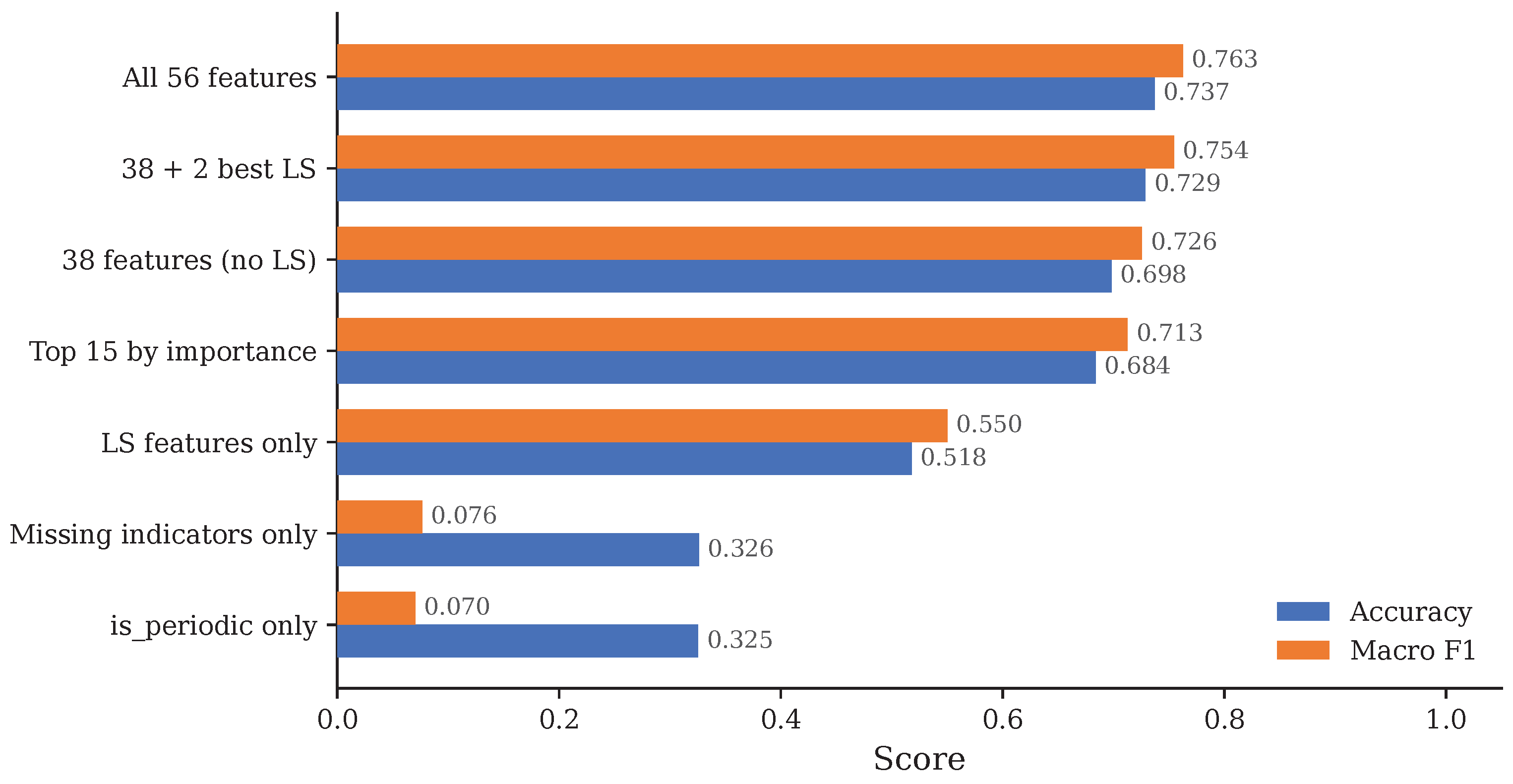
Controlled feature-group ablation (50K subset, fixed hyperparameters, main 56/38 catalogs). Bars show test accuracy and macro F1 for each subset (values annotated). Under this protocol the full 56-feature set is strongest; adding only ls_peak_width and ls_dominant_period to the 38-feature set recovers most of the drop. See Section 4.2.2 for the full-scale comparison.
Under this controlled protocol:
- The full 56-feature set is strongest on the 50K subset (accuracy = 0.737; macro F1 = 0.763). Absolute scores lie well below Table 2 because of the smaller sample and fixed hyperparameters.
- Removing the LS periodogram block, is_periodic, and missing-value indicators decreases accuracy by about 3.9 percentage points (macro F1 by 3.7 percentage points). Adding back only ls_peak_width and ls_dominant_period recovers most of that drop (accuracy = 0.729; macro F1 = 0.754).
- LS periodogram features alone reach accuracy = 0.518 (macro F1 = 0.550)—above chance but insufficient as a standalone classifier.
- Missing-value indicators alone, and the single feature is_periodic, remain near chance (accuracy ≈ 0.33; macro F1 ≈ 0.07), so they are supplementary rather than primary discriminators in this subset study.
Under the same 50K fixed-hyperparameter protocol, adding ndethist changes neither the 56-feature run (0.737 in both cases) nor the 38-feature no-LS run (∼0.698 in both cases). The same conclusion holds on the full Optuna-tuned benchmark; the 38-feature vs. 39-feature comparison is reported in Appendix C.1.
Appendix C.1. Metadata Proxy Analysis
Table A7 shows that adding the fallback ndethist column to XGBoost-Reduced changes test accuracy by less than 0.01 percentage points when both models reuse the Optuna hyperparameters of Table A2 (no re-tuning). This negligible difference, combined with the fact that the column is constructed from segment length and survey origin rather than from photometric morphology, motivates omitting ndethist from the main models.
Table A7.
Effect of adding ndethist to XGBoost-Reduced. Both rows reuse the Optuna hyperparameters of Table A2 (no re-tuning).
Future work should (i) join true ZTF ndethist from alert packets at the parent-source level if exposure-history metadata are desired, and (ii) report SN metrics on independent, single-survey validation sets without resampling augmentation.
Appendix C.2. Feature Importance: Full vs. Reduced Models
Figure A2 compares the top feature importances for XGBoost-Full and XGBoost-Reduced. Removing LS-related descriptors increases the relative weight of variability-amplitude features such as excess_variance and w_std_mag.
Figure A2.
Top 15 XGBoost feature importances for XGBoost-Full (56 features; left) and XGBoost-Reduced (38 features, no LS; right). Removing LS-related descriptors increases the relative weight of variability-amplitude features such as excess_variance and w_std_mag.
Appendix C.3. Feature Category Importance
Figure A3 presents the aggregated feature importance by category from XGBoost-Full (56 features). The 18 columns present only in XGBoost-Full account for 35.1% of total importance. As shown in Section 4.2.2, this share does not yield a robust full-scale accuracy gain.
Figure A3.
Aggregated feature importance by category from XGBoost-Full (56 features). The 18 columns present only relative to XGBoost-Reduced account for 35.1% of total importance. Displayed percentages sum to 100.1% due to rounding.
Appendix C.4. LS Feature Reliability Across Observation Regimes
Figure A4 quantifies how the impact of LS features evolves with observation count. The per-count Reduced − Full gap is largest near 3–8 observations (mean about percentage points) and falls to near zero (slightly negative) by 23–30 observations, showing that any LS contribution is strongly sampling dependent. This trend is consistent with the need for adequate phase coverage in periodogram analysis [23]. Our benchmark is restricted to 3–30 epochs. The ≥15-point control summarized in Section 4.2.2 likewise finds no robust Full advantage. Whether LS descriptors become net beneficial beyond 30 epochs remains an open question for future work.
Figure A4.
LS feature impact across observation counts (38 vs. 56 features). Per-count accuracy difference (Reduced − Full; light) and three-point rolling mean (dark). The advantage of omitting LS descriptors is largest at low observation counts and fades toward zero by 23–30 observations.
Appendix D. Additional Computational Benchmarks
Table A8 provides complete CPU inference benchmarks, and Table A9 provides complete GPU benchmarks for all models.
Table A8.
CPU inference benchmarks (257,742 test samples). Feature extraction times for XGBoost-Full and the Feature-based Transformer are shared because both use the same LS-inclusive varlen feature pipeline (56 features in the main models); timings are from a CPU-only benchmark with 1000-sample extrapolation to the full test set (Appendix D).
For Feature-based Transformer models, feature extraction is performed on CPU and dominates total processing time even when inference runs on GPU. All benchmarks use the full 257,742-sample test set; Figure 9a reports the same totals normalized to per 10k samples.
Figure A5.
CPU vs. GPU inference time comparison. Deep-learning models benefit from GPU acceleration, whereas GPU offloading provides no speedup for the XGBoost pipeline evaluated here.
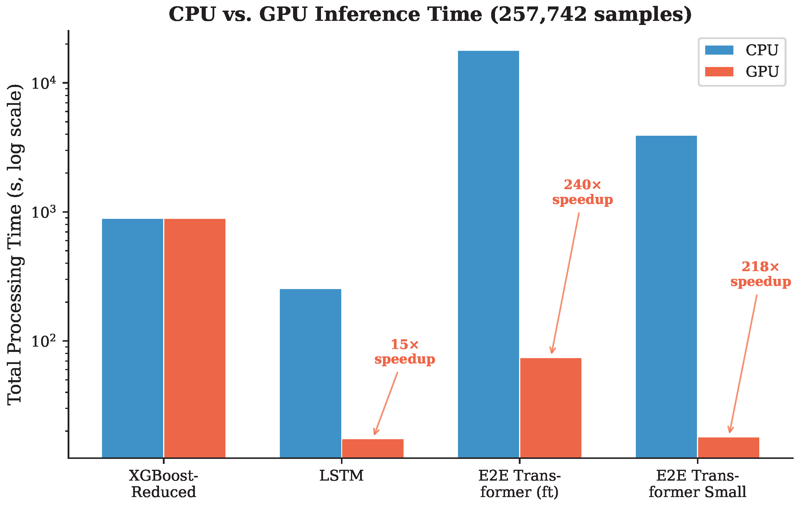
Figure A6.
Training wall-clock time comparison. Times are measured from training-log epoch timestamps (not whole-log file spans). The LSTM completes training fastest (1.7 h for 100 epochs). E2E Transformer 50-observation pre-training is the most expensive single stage (76 h for 89 epochs).
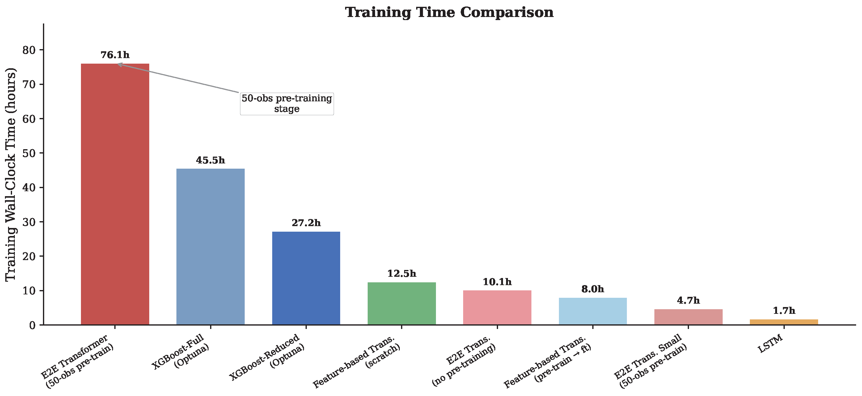
Table A9.
GPU and mixed-deployment inference benchmarks (257,742 test samples). XGBoost rows use CPU for both feature extraction and inference. Feature-based Transformer feature extraction (994.1 s) was measured in a separate end-to-end production benchmark on the full test set (cf. the CPU extrapolation in Table A8).
Per-Class F1 Scores
Figure A7.
Per-class F1 scores for the three best-performing models with distinct architectures. Supernova F1 is near ceiling on this benchmark for all three methods (see Section 2.2 for construction caveats), while Active stars and Pulsating variables remain the most challenging classes.
Appendix E. Confusion Matrix for XGBoost-Full
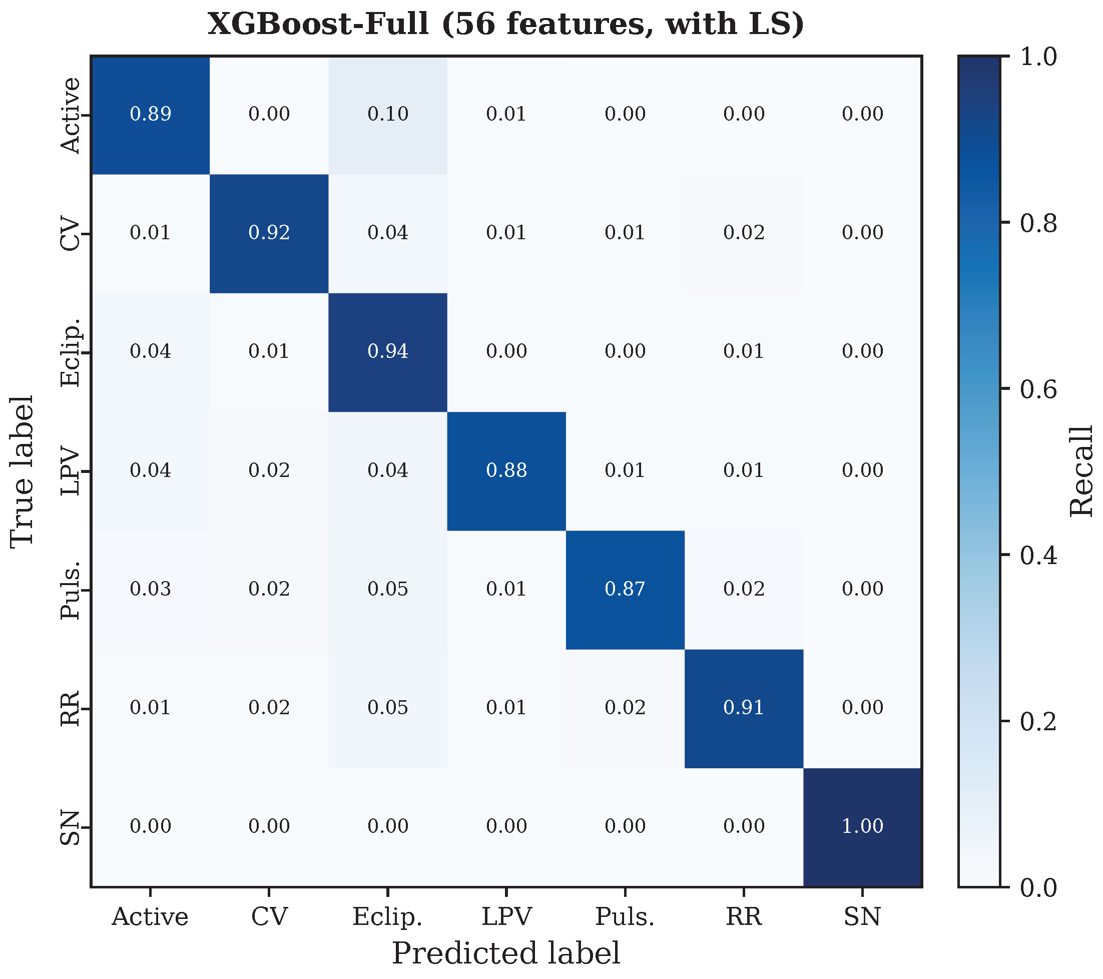
Figure A8 presents the confusion matrix for XGBoost-Full (56 features, including all LS periodogram features and associated missing-value indicators). Compared with XGBoost-Reduced (Figure 4a), the overall pattern is similar and per-class recalls are comparable, with XGBoost-Reduced equal or slightly higher for Active (0.90 vs. 0.89), CV (0.923 vs. 0.917), and Pulsating (0.89 vs. 0.87). The main difference is somewhat increased Active-to-Eclipsing misclassification in XGBoost-Full (9.8% vs. 8.6%). XGBoost-Full nevertheless achieves a marginally lower macro F1 (0.923 vs. 0.931), consistent with the small full-scale performance gap reported in Table 2.
Figure A8.
Confusion matrix for XGBoost-Full (56 features, with LS). Values represent row-normalized recall fractions. The pattern is broadly similar to XGBoost-Reduced (Figure 4a), with marginally lower test accuracy (0.913 vs. 0.922).
Appendix F. Confusion Matrices for Additional Transformer Models
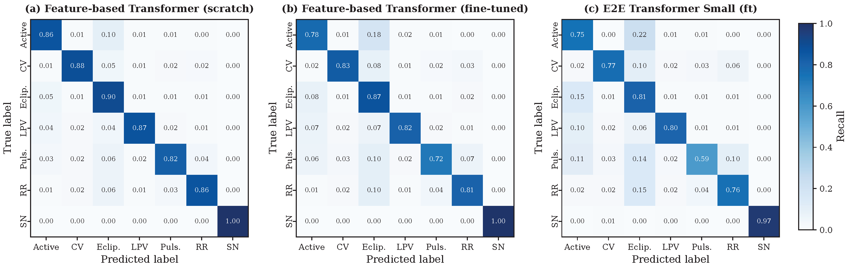
Figure A9 presents row-normalized confusion matrices for the three Transformer variants omitted from Figure 4. The Feature-based Transformer from scratch (Figure A9a) achieves test accuracy 0.878 on the 56-feature inputs, with moderate Active–Eclipsing confusion and near-perfect SN recall. Fine-tuning from a 50-observation pre-trained checkpoint (Figure A9b) degrades performance to 0.823, with increased misclassification among Active, Pulsating, and RR classes—consistent with the negative transfer reported in Table 2. The lightweight E2E Transformer Small (Figure A9c; 10.2 M parameters) reaches test accuracy 0.764 after pre-training and fine-tuning, substantially below the full-size E2E Transformer (Figure 4b; accuracy 0.946).
Figure A9.
Confusion matrices for additional Transformer models. (a) Feature-based Transformer trained from scratch on 56 handcrafted features (test accuracy 0.878). (b) Feature-based Transformer fine-tuned from a 50-observation pre-trained checkpoint (test accuracy 0.823). (c) E2E Transformer Small (10.2 M parameters) after pre-training and fine-tuning on variable-length sequences (test accuracy 0.764). Values represent row-normalized recall fractions; layout and color scale match Figure 4.
Appendix G. Accuracy vs. Observation Count for Additional Models
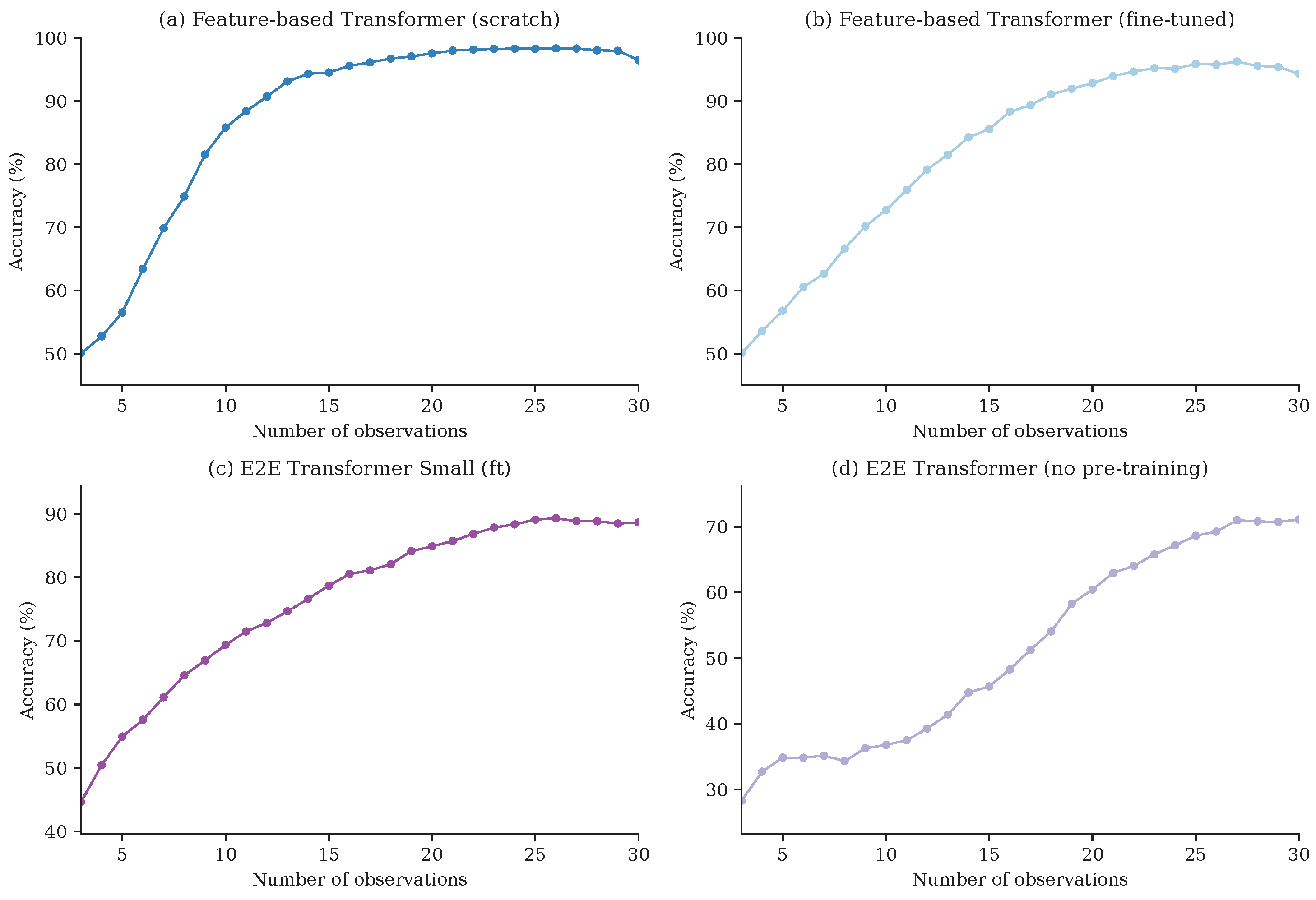
Figure A10 presents the per-observation-count accuracy curves for four additional models, complementing the curves shown in Figure 6 in the main text (which focuses on three representative architectures in Figure 6b and the two XGBoost variants in Figure 6a). Figure A10a shows the Feature-based Transformer trained from scratch on 56-feature inputs, which exhibits a steady improvement from ∼0.50 at 3 observations to ∼0.96 at 30 observations—a ∼46 percentage-point gain, comparable in magnitude to the LSTM baseline (Section 4.4). Figure A10b shows the fine-tuned Feature-based Transformer, which underperforms the from-scratch model on the full test set from five observations upward (by up to ∼13 percentage points at intermediate counts), with only a marginal advantage near four observations. Figure A10c shows the lightweight E2E Transformer Small, which benefits from pre-training (rising from ∼0.45 at 3 obs to ∼0.89 at 30 obs), but remains 10–15 percentage points below the full-size E2E Transformer at every observation count. Figure A10d confirms that the E2E Transformer without pre-training barely exceeds 70% accuracy even at 30 observations, underscoring that model capacity alone is insufficient without transfer learning in the sparse regime.
Figure A10.
Classification accuracy as a function of observation count for four additional models. (a) Feature-based Transformer from scratch. (b) Feature-based Transformer fine-tuned. (c) E2E Transformer Small (pre-trained then fine-tuned). (d) E2E Transformer without pre-training. The y-axis ranges differ between panels to highlight individual trends.
References
- Leavitt, H.S.; Pickering, E.C. Periods of 25 Variable Stars in the Small Magellanic Cloud. Harv. Coll. Obs. Circ. 1912, 173, 1–3. [Google Scholar]
- Riess, A.G.; Filippenko, A.V.; Challis, P.; Clocchiatti, A.; Diercks, A.; Garnavich, P.M.; Gilliland, R.L.; Hogan, C.J.; Jha, S.; Kirshner, R.P.; et al. Observational Evidence from Supernovae for an Accelerating Universe and a Cosmological Constant. Astron. J. 1998, 116, 1009–1038. [Google Scholar] [CrossRef] [Scilit]
- Koch, D.G.; Borucki, W.J.; Basri, G.; Batalha, N.M.; Brown, T.M.; Caldwell, D.; Christensen-Dalsgaard, J.; Cochran, W.D.; DeVore, E.; Dunham, E.W.; et al. Kepler Mission Design, Realized Photometric Performance, and Early Science. Astrophys. J. Lett. 2010, 713, L79–L86. [Google Scholar] [CrossRef] [Scilit]
- Holoien, T.W.-S.; Stanek, K.Z.; Kochanek, C.S.; Shappee, B.J.; Prieto, J.L.; Brimacombe, J.; Bersier, D.; Babusiaux, C.; Bailer-Jones, C.A.L.; Bastian, U.; et al. The ASAS-SN Bright Supernova Catalogue—I. 2013–2014. Mon. Not. R. Astron. Soc. 2017, 464, 2672–2686. [Google Scholar] [CrossRef] [Scilit]
- Kochanek, C.S.; Shappee, B.J.; Stanek, K.Z.; Holoien, T.W.-S.; Thompson, T.A.; Prieto, J.L.; Dong, S.; Shields, J.V.; Will, D.; Britt, C.; et al. The All-Sky Automated Survey for Supernovae (ASAS-SN) Light Curve Server v1.0. Publ. Astron. Soc. Pac. 2017, 129, 104502. [Google Scholar] [CrossRef] [Scilit]
- Gaia Collaboration. Gaia Data Release 1. Summary of the Astrometric, Photometric, and Survey Properties. Astron. Astrophys. 2016, 595, A2. [Google Scholar] [CrossRef] [Scilit]
- Bellm, E.C.; Kulkarni, S.R.; Graham, M.J.; Dekany, R.; Smith, R.M.; Riddle, R.; Masci, F.J.; Helou, G.; Prince, T.A.; Adams, S.M.; et al. The Zwicky Transient Facility: System Overview, Performance, and First Results. Publ. Astron. Soc. Pac. 2019, 131, 018002. [Google Scholar] [CrossRef] [Scilit]
- Ricker, G.R.; Winn, J.N.; Vanderspek, R.; Latham, D.W.; Bakos, G.Á.; Bean, J.L.; Berta-Thompson, Z.K.; Brown, T.M.; Buchhave, L.; Butler, N.R.; et al. Transiting Exoplanet Survey Satellite (TESS). J. Astron. Telesc. Instrum. Syst. 2015, 1, 014003. [Google Scholar] [CrossRef] [Scilit]
- Ivezić, Ž.; Kahn, S.M.; Tyson, J.A.; Abel, B.; Acosta, E.; Allsman, R.; AlSayyad, Y.; Anderson, S.F.; Andrew, J.; Angel, J.R.P.; et al. LSST: From Science Drivers to Reference Design and Anticipated Data Products. Astrophys. J. 2019, 873, 111. [Google Scholar] [CrossRef] [Scilit]
- Richards, J.W.; Starr, D.L.; Butler, N.R.; Bloom, J.S.; Brewer, J.M.; Crellin-Quick, A.; Higgins, J.; Kennedy, R.; Rischard, M. On Machine-learned Classification of Variable Stars with Sparse and Noisy Time-series Data. Astrophys. J. 2011, 733, 10. [Google Scholar] [CrossRef] [Scilit]
- Richards, J.W.; Starr, D.L.; Miller, A.A.; Bloom, J.S.; Butler, N.R.; Brink, H.; Crellin-Quick, A. Construction of a Calibrated Probabilistic Classification Catalog: Application to 50k Variable Sources in the All-Sky Automated Survey. Astrophys. J. Suppl. Ser. 2012, 203, 32. [Google Scholar] [CrossRef] [Scilit][Green Version]
- Nun, I.; Protopapas, P.; Sim, B.; Zhu, M.; Dave, R.; Castro, N.; Pichara, K. FATS: Feature Analysis for Time Series. arXiv 2015, arXiv:1506.00010. [Google Scholar] [CrossRef] [Scilit]
- Muthukrishna, D.; Narayan, G.; Mandel, K.S.; Biswas, R.; Hložek, R. RAPID: Early Classification of Explosive Transients Using Deep Learning. Publ. Astron. Soc. Pac. 2019, 131, 118002. [Google Scholar] [CrossRef] [Scilit]
- Villar, V.A.; Hosseinzadeh, G.; Berger, E.; Ntampaka, M.; Jones, D.O.; Challis, P.; Chornock, R.; Drout, M.R.; Foley, R.J.; Kirshner, R.P. SuperRAENN: A Semisupervised Supernova Photometric Classification Pipeline Trained on Pan-STARRS1 Medium-Deep Survey Supernovae. Astrophys. J. 2020, 905, 94. [Google Scholar] [CrossRef] [Scilit]
- Allam, T.; McEwen, J.D. Paying Attention to Astronomical Transients: Introducing the Time-series Transformer for Photometric Classification. RAS Tech. Instrum. 2024, 3, 209–223. [Google Scholar] [CrossRef] [Scilit]
- Donoso-Oliva, C.; Becker, I.; Protopapas, P.; Cabrera-Vives, G.; Vishnu, M.; Vardhan, H. ASTROMER: A Transformer-based Embedding for the Representation of Light Curves. Astron. Astrophys. 2023, 670, A54. [Google Scholar] [CrossRef] [Scilit]
- Hochreiter, S.; Schmidhuber, J. Long Short-Term Memory. Neural Comput. 1997, 9, 1735–1780. [Google Scholar] [CrossRef] [Scilit] [PubMed]
- Vaswani, A.; Shazeer, N.; Parmar, N.; Uszkoreit, J.; Jones, L.; Gomez, A.N.; Kaiser, Ł.; Polosukhin, I. Attention is All You Need. In Proceedings of the 31st International Conference on Neural Information Processing Systems (NeurIPS); Curran Associates, Inc.: Red Hook, NY, USA, 2017; pp. 5998–6008. [Google Scholar] [CrossRef] [Scilit]
- Tonry, J.L.; Denneau, L.; Heinze, A.N.; Stalder, B.; Smith, K.W.; Smartt, S.J.; Stubbs, C.W.; Weiland, H.J.; Rest, A. ATLAS: A High-cadence All-sky Survey System. Publ. Astron. Soc. Pac. 2018, 130, 064505. [Google Scholar] [CrossRef] [Scilit]
- Chen, X.; Wang, S.; Deng, L.; de Grijs, R.; Yang, M.; Tian, H. The Zwicky Transient Facility Catalog of Periodic Variable Stars. Astrophys. J. Suppl. Ser. 2020, 249, 18. [Google Scholar] [CrossRef] [Scilit]
- ZTF Team. ZTF Lightcurves; IPAC: Pasadena, CA, USA, 2025. [Google Scholar] [CrossRef]
- Masci, F.J.; Laher, R.R.; Rusholme, B.; Shupe, D.L.; Groom, S.; Surace, J.; Jackson, E.; Monkewitz, S.; Beck, R.; Flynn, D.; et al. The Zwicky Transient Facility: Data Processing, Products, and Archive. Publ. Astron. Soc. Pac. 2019, 131, 018003. [Google Scholar] [CrossRef] [Scilit]
- VanderPlas, J.T. Understanding the Lomb–Scargle Periodogram. Astrophys. J. Suppl. Ser. 2018, 236, 16. [Google Scholar] [CrossRef] [Scilit]
- Stetson, P.B. On the Automatic Determination of Light-Curve Parameters for Cepheid Variables. Publ. Astron. Soc. Pac. 1996, 108, 851–866. [Google Scholar] [CrossRef] [Scilit] [PubMed]
- Nordin, J.; Brinnel, V.; van Santen, J.; Bulla, M.; Feindt, U.; Franckowiak, A.; Fremling, C.; Gal-Yam, A.; Giomi, M.; Kowalski, M.; et al. Transient Processing and Analysis Using AMPEL: Alert Management, Photometry, and Evaluation of Light Curves. Astron. Astrophys. 2019, 631, A147. [Google Scholar] [CrossRef] [Scilit]
- Van Ness, M.; Bosschieter, T.M.; Halpin-Gregorio, R.; Udell, M. The Missing Indicator Method: From Low to High Dimensions. In Proceedings of the 29th ACM SIGKDD Conference on Knowledge Discovery and Data Mining; ACM: New York, NY, USA, 2023; pp. 5004–5015. [Google Scholar] [CrossRef] [Scilit]
- Chen, T.; Guestrin, C. XGBoost: A Scalable Tree Boosting System. In Proceedings of the 22nd ACM SIGKDD International Conference on Knowledge Discovery and Data Mining; ACM: New York, NY, USA, 2016; pp. 785–794. [Google Scholar] [CrossRef] [Scilit]
- Akiba, T.; Sano, S.; Yanase, T.; Ohta, T.; Koyama, M. Optuna: A Next-generation Hyperparameter Optimization Framework. In Proceedings of the 25th ACM SIGKDD International Conference on Knowledge Discovery & Data Mining; ACM: New York, NY, USA, 2019; pp. 2623–2631. [Google Scholar] [CrossRef] [Scilit]
- Grinsztajn, L.; Oyallon, E.; Varoquaux, G. Why Do Tree-Based Models Still Outperform Deep Learning on Typical Tabular Data? In Advances in Neural Information Processing Systems 35 (NeurIPS); Curran Associates, Inc.: Red Hook, NY, USA, 2022; pp. 507–520. [Google Scholar] [CrossRef] [Scilit]
- Strobl, C.; Boulesteix, A.-L.; Zeileis, A.; Hothorn, T. Bias in Random Forest Variable Importance Measures: Illustrations, Sources and a Solution. BMC Bioinform. 2007, 8, 25. [Google Scholar] [CrossRef] [Scilit] [PubMed]
- Gregorutti, B.; Michel, B.; Saint-Pierre, P. Correlation and Variable Importance in Random Forests. Stat. Comput. 2017, 27, 659–678. [Google Scholar] [CrossRef] [Scilit]
- Gautschy, A.; Saio, H. Stellar Pulsations Across the HR Diagram. Annu. Rev. Astron. Astrophys. 1995, 33, 75–114. [Google Scholar] [CrossRef]
- Schmidt, E.G. The Behlen Observatory Variable Star Survey: First Results. Astron. J. 1991, 102, 1766–1776. [Google Scholar] [CrossRef] [Scilit] [PubMed][Green Version]
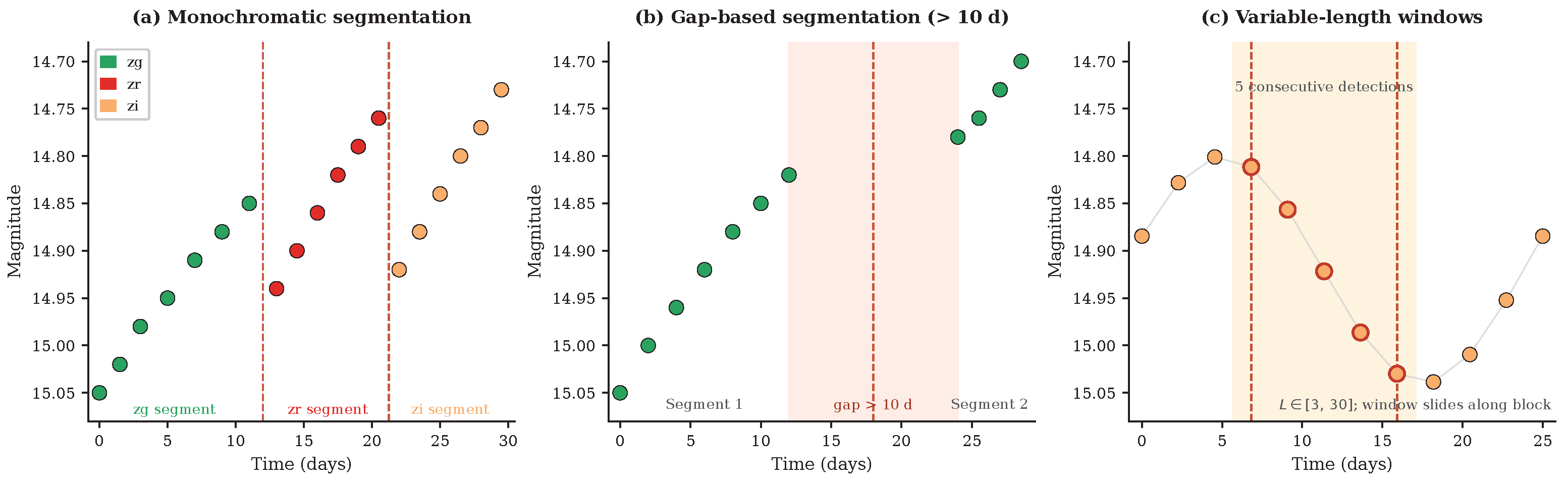
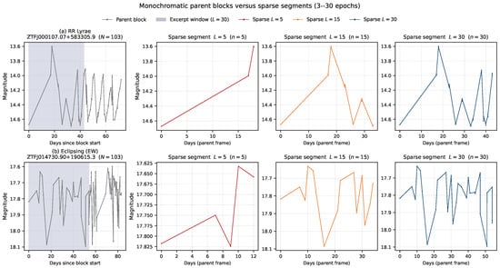
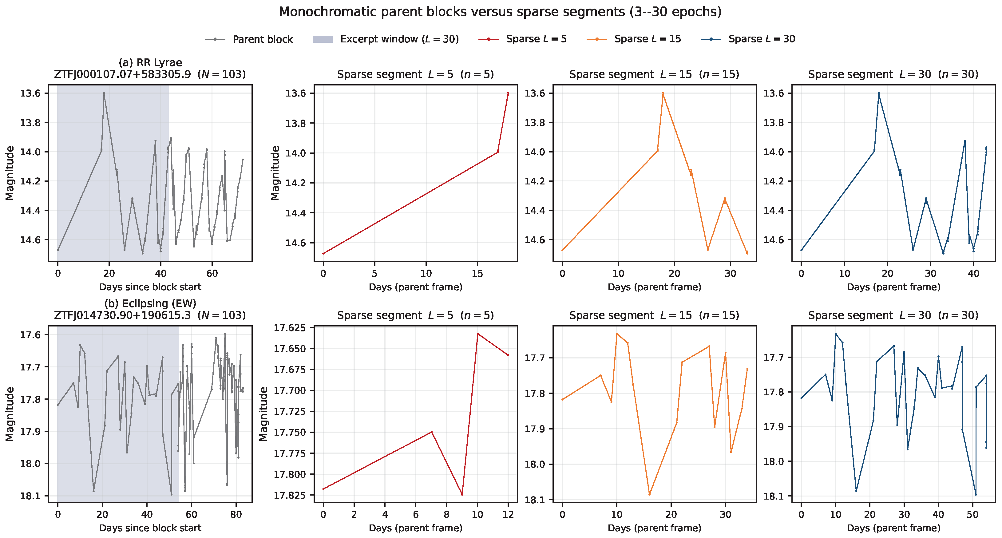
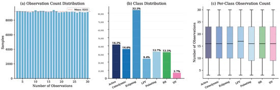
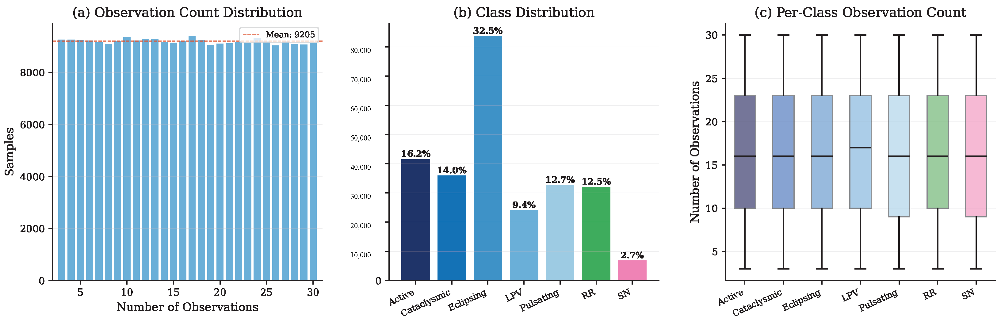
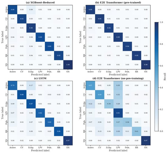
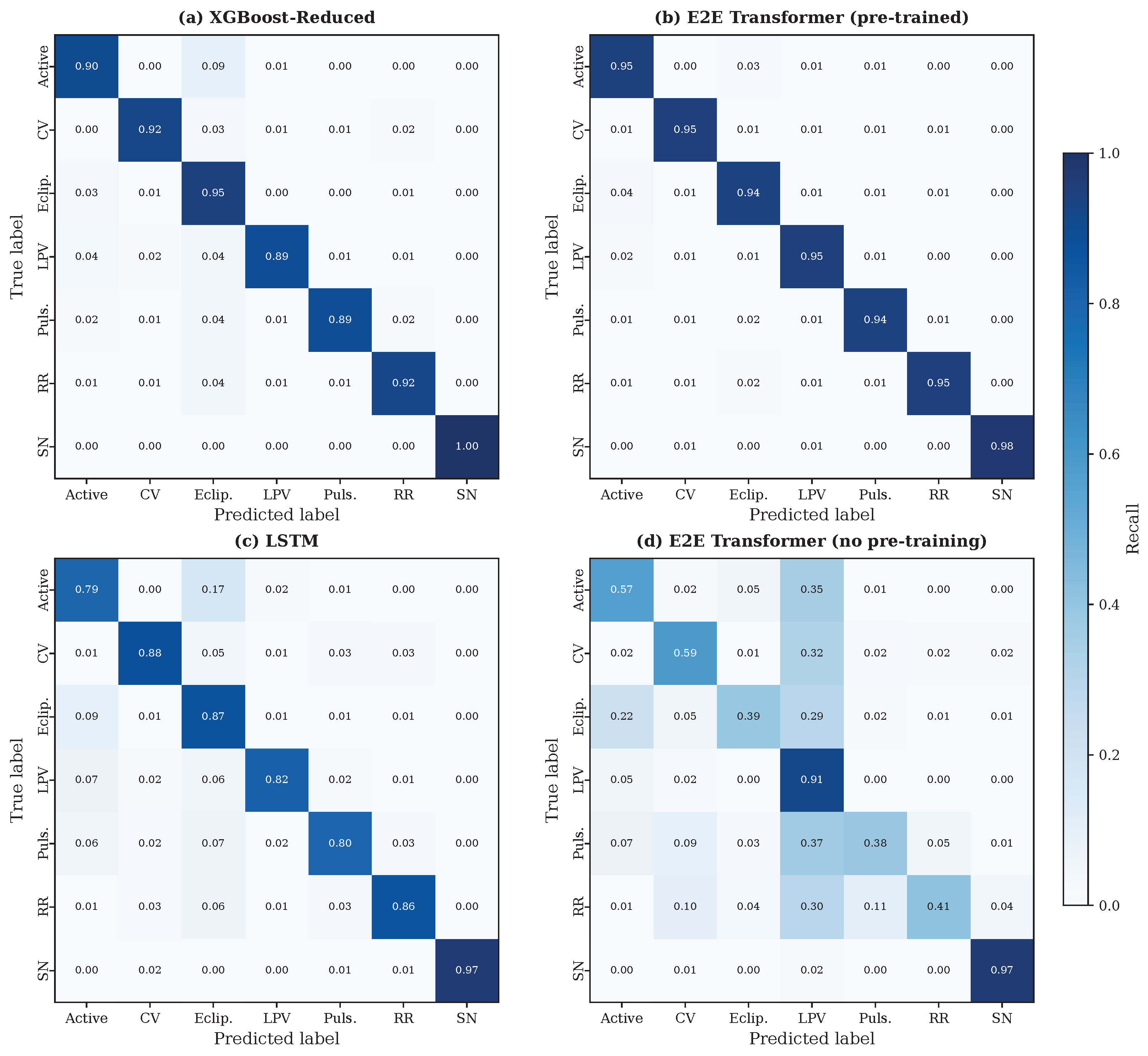
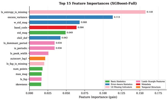
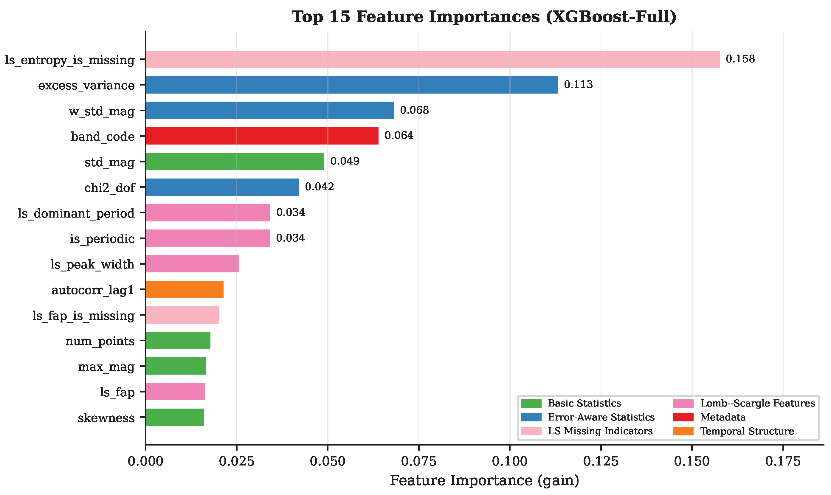
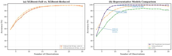
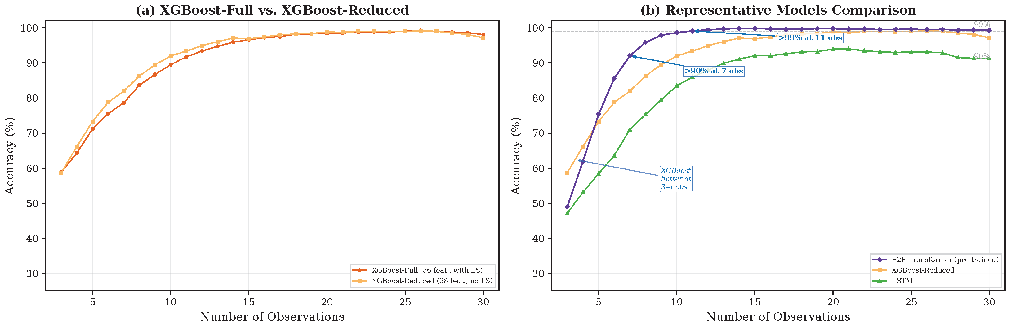
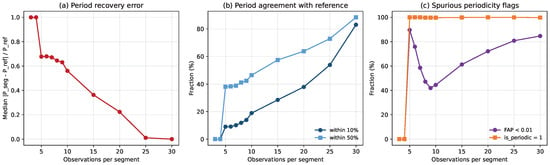
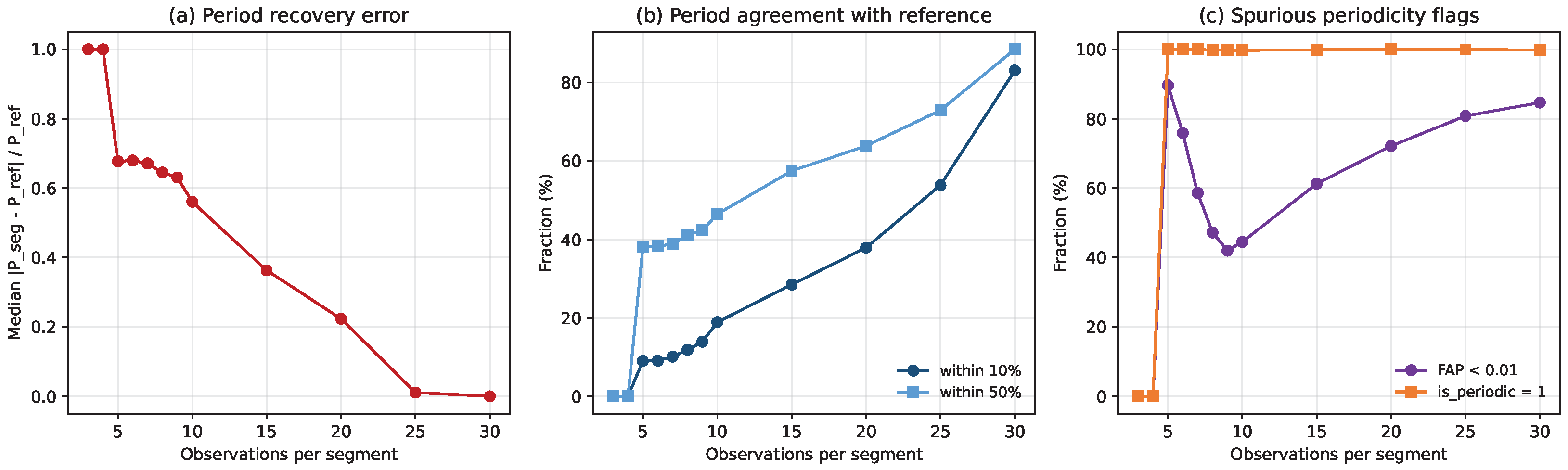
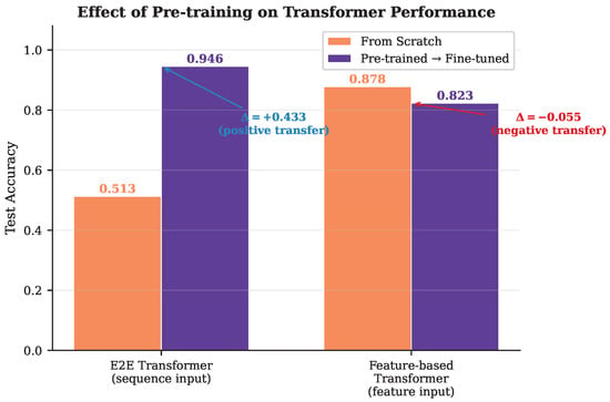
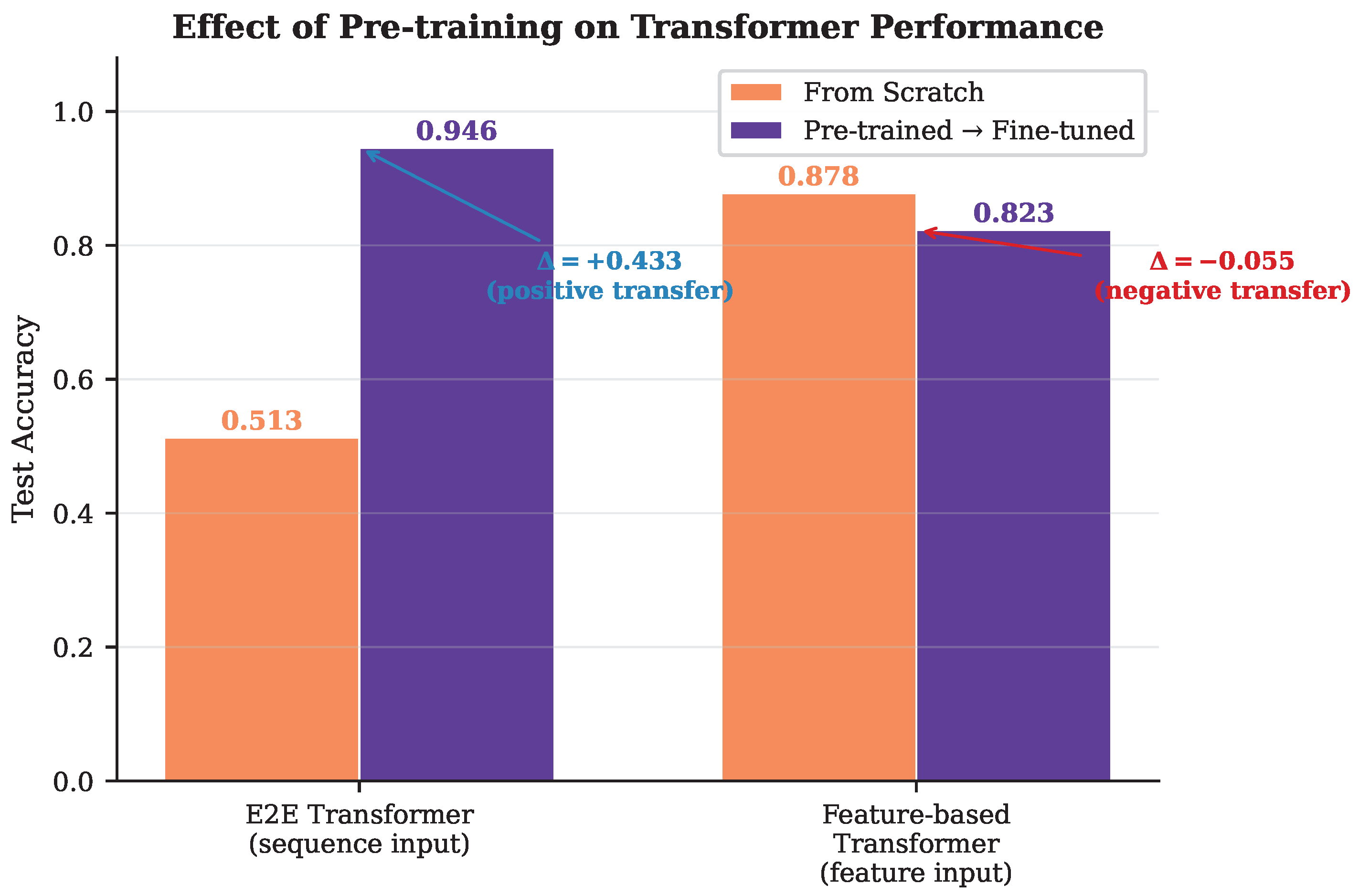
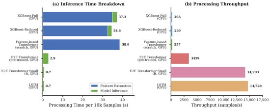
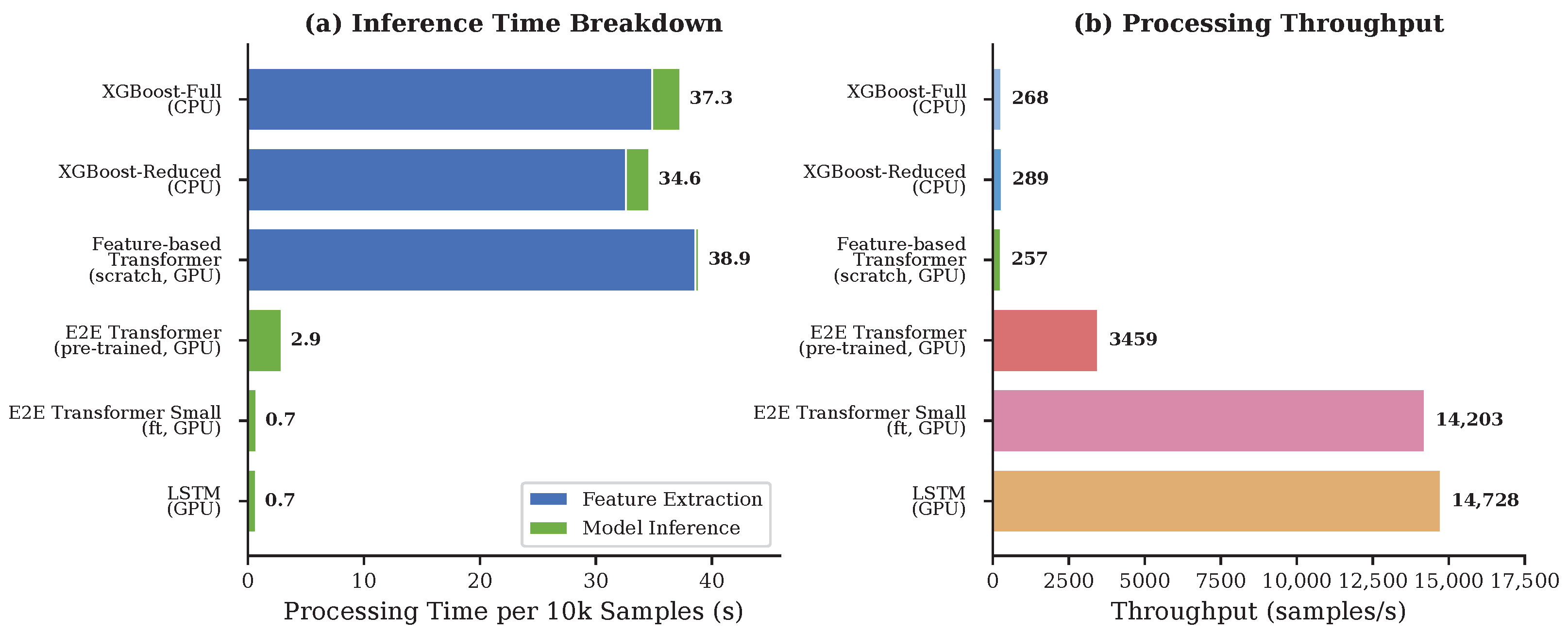
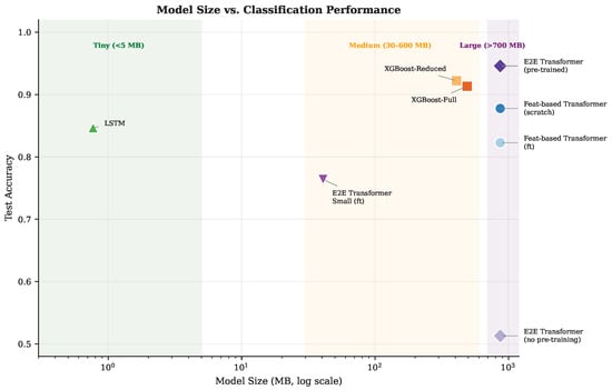
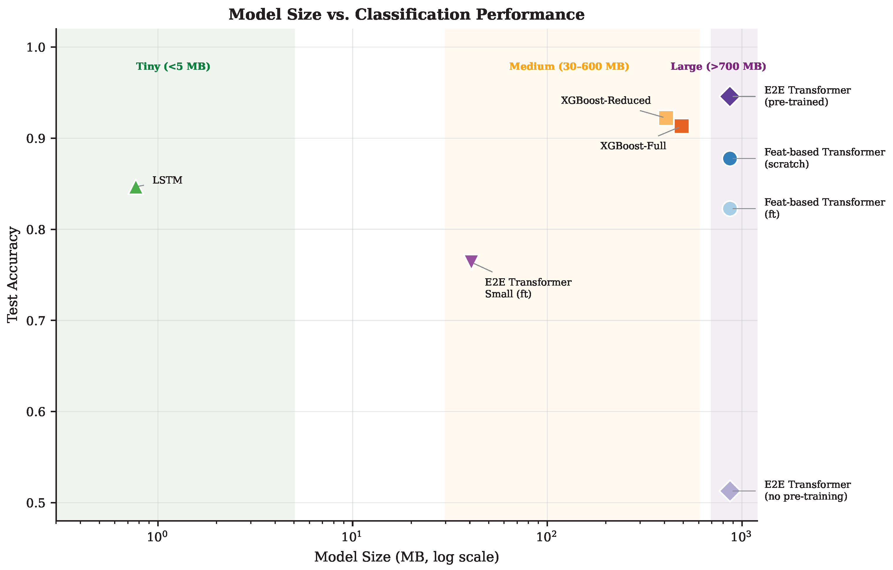

Disclaimer/Publisher’s Note: The statements, opinions and data contained in all publications are solely those of the individual author(s) and contributor(s) and not of MDPI and/or the editor(s). MDPI and/or the editor(s) disclaim responsibility for any injury to people or property resulting from any ideas, methods, instructions or products referred to in the content. |
© 2026 by the authors. Licensee MDPI, Basel, Switzerland. This article is an open access article distributed under the terms and conditions of the Creative Commons Attribution (CC BY) license.