Some Remarks on the Horizon in the Dust Cloud Collapse

Abstract

We examine the existence of an apparent horizon in the collapse of an isolated dust cloud in spherically symmetric spacetime. The interior geometry is expressed in the Lemaître–Tolman–Bondi coordinates, while the outside geometry is the standard Schwarzschild. The novelty of the approach lies in using the Lemaître coordinates for the Schwarzschild part of the geometry when discussing junction conditions. We provide general formulas for expansions in the marginally bound cloud case and use them to determine the position of the apparent horizon. Our results indicate that in the region of spacetime far from the gravitational singularity, the system under consideration has a horizon, and thus the singularity is not naked. The results are expected to be correct away from the singularity, where quantum effects can be neglected. Near the singularity, general relativity breaks down, and quantum gravity would be of primary importance. The classical formulas for expansion scalars can serve as a starting point for more detailed quantum analysis.

1. Introduction

Within a year of Einstein’s equations coming into existence, an exact solution to them were found in Schwarzschild’s solution. And this was a boon and a bane, since it contained a singularity at its center. Despite this result, singularities, for a long time, were considered to be the artifacts of stringent symmetric conditions. Following that, Hawking, Geroch and Penrose’s singularity theorems [1] proved that singularities are fundamental geometric features of all generic spacetimes except the Minkowskian flat spacetime. However fundamental these features are, they are problematic since they are the edges of the otherwise smooth, paracompact, Hausdroff spacetime manifolds [2], and the maximal Cauchy developments of inextendible non-spacelike geodesics on these manifolds are truncated at these edges. Therefore, spacetime singularities are generic and irremovable features of general relativity and the biggest problem surrounding these objects is their genericity and visibility, the latter of which we discuss in this work.

Schwarzschild’s solution and the singularity contained in it is a unique solution for vacuum, asymptotically flat, static, spherically symmetric spacetimes [3]. This specific solution can also be obtained from the collapse of a spherically symmetric, pressureless and homogeneous dust cloud [4,5]. This work also showed that an event horizon1 would form before the formation of this spacelike singularity and so, any causal connection in the direction of the future from this is automatically prohibited: this singularity is a black hole. Also, this singularity is gravitationally strong [6]: any object would be crushed to zero volume on approaching this.

Following the flawless structure of the Schawarzschild black hole, it was hypothesised by Penrose [7,8] that all spacetime singularities should be hidden behind event horizons and no future directed non-spacelike geodesic is allowed to escape from the its neighbourhood. However, there is no proof for this theorem—Cosmic Censorship Conjecture—but it was assumed to be overarchingly true in the classical theory of gravity. It is important to emphasize at this point that the singularity theorems do not necessitate the existence of trapped surfaces or horizons for the existence of an incomplete non-spacelike geodesic, which is a necessary and sufficient condition for a singularity to exist. Following this, multiple different physically reasonable matter fields (of types I and II [1]) were investigated to resolve the issue of visibility in spacetime singularities and some counter-intuitive results were obtained. Christodoulou found that a singularity can be formed from a dust cloud collapse when there are no horizons forming [9]. Later works also confirmed these results [10,11]. It was shown that the inhomogeneous, self-similar, marginally bound, pressureless dust, after going through a continual collapse, produces a singularity where a local or apparent horizon is formed at the same instance when the singularity forms. Investigation of the null geodesics showed that, unlike a black hole, the tangents to the future directed ones were positive definite [12], and thus it was structurally different from a black hole: a naked singularity. Based on these findings, a precise definition of a naked singularity was given: if there exists a family of inextendible outgoing non-spacelike geodesics in a spacetime, whose causal past lies in the neighbourhood of the singularity, then it is at least locally naked. These results were also obtained for non-self-similar cases [13,14] as well as non-marginally bound cases [15]. The results regarding an end-state singularity stayed qualitatively similar when the pressure was turned on in the collapsing cloud [16,17,18,19]. However, these naked singularity results only regard visibility locally, without discussing whether the geodesics are future complete, i.e., whether they will reach an observer at asymptotic distance.

Global visibility is important for observational purposes, since locally naked singularities would be more difficult to locate and gather signals from using distant probes. There are enough examples of globally naked singularities [20,21,22,23,24,25]. More importantly, these models have found relevance in recent observational studies: the central compact object of the Sgr A* was stipulated as either a black-hole or a naked singularity [26]. Naked singularities have found substantial support from different studies involving simulations, for instance, accretion flows [27,28,29], shadows [30,31], precession orbits [32,33], etc.

Naked singularities are globally important since their existence allows very strong gravity regimes to come into causal contact with even asymptotic observers since there is no horizon prohibiting this contact. As quantum gravitational effects are said to become important at such length and energy scales, their direct observation becomes possible if the singularity is globally visible. Quantum approaches have been applied to gravitational collapse scenarios of homogeneous, pressureless, spherically symmetric clouds [34,35]. A similar approach has been applied to a homogeneous collapsing cloud with non-zero isotropic pressure [36], in which the singularity evaporates upon the application of the quantum theory. So, the next natural step would be to apply quantum theory to a more complex collapsing scenario: an inhomogeneous, but pressureless, collapsing cloud. The reason to explore this direction is to find the fate of gravitational singularities at the quantum level. This would also help to construct a satisfactory theory of quantum gravity.

We build on the same premise in the present work and reinvestigate the features of inhomogeneous, pressureless, spherically symmetric, marginally bound dust. The aim of this paper is to examine the existence of the horizon and the trapped region of the isolated collapsing cloud of dust using expansion functions, since we are interested in astrophysically relevant naked singularities, where horizons do not form at all. In what follows, we set $8\pi G/c^4=1.$

2. The LTB Spacetime

The gravitational collapse of a spherically symmetric, inhomogeneous and marginally bound cloud of dust can be described by the Lemaître–Tolman–Bondi Equation [12,14,37]:

$$\begin{array}{c}\hfill d{s}^2=-d{t}^2+{\left(R^{\prime }\right)}^{2}d{r}^2+R^2(d{\theta }^2+{sin}^2\theta d{\varphi }^2),\end{array}$$

(1)

where $R=R(t,r)$ is the area radius at time t of the shell with radial coordinate r, and where $R^{\prime }=\partial R/\partial r$. The energy-momentum tensor $T^{\mu \nu }=\rho (t,r)U^{\mu }{U}^{\nu }$, where $\rho (t,r)$ is the energy density of the cloud and $U^{\mu }$ is the four velocity.

Inserting Equation (1) into the Einstein equations leads to

$${\dot{R}}^2={\displaystyle \frac{F}{R}}$$

(2)

and

$$\rho ={\displaystyle \frac{F^{\prime }}{R^2{R}^{\prime }}},$$

(3)

where $\dot{R}=\partial R/\partial t$, and where $F=F\left(r\right)$ is the mass of the cloud inside the shell of coordinate r.

The case of collapse is described by $R^{\prime }<0$, where R is the physical radius of the collapsing configuration. The shell index r can be calculated using $R(0,r)=r$.

Integrating (2) gives

$$\begin{array}{c}\hfill R^{{\displaystyle \frac{3}{2}}}=r^{{\displaystyle \frac{3}{2}}}-{\displaystyle \frac{3}{2}}t\sqrt{F}.\end{array}$$

(4)

The solution to (3) can be found to be

$$\begin{array}{c}\hfill \rho (t,r)={\displaystyle \frac{4\sqrt{F\left(r\right)}{F}^{\prime }\left(r\right)}{\left(3t\sqrt{F\left(r\right)}-2r^{3/2}\right)}}{\displaystyle \frac{1}{\left(t{F}^{\prime }\left(r\right)-2\sqrt{rF\left(r\right)}\right)}}.\end{array}$$

(5)

For details, see Appendix A.

3. Apparent Horizon

Let $\Sigma$ stand for a codimension-two hypersurface embedded in a four-dimensional spacetime. The normal space for such a surface is spanned by a pair of null vectors $l^{\mu }$ and $n^{\mu }$. Assuming they are cross-normalized, $l·n=-1$, the induced metric on $\Sigma$ reads [38,39,40]

$$\begin{array}{c}\hfill q_{\mu \nu }=g_{\mu \nu }+l_{\mu }{n}_{\nu }+l_{\nu }{n}_{\mu },\end{array}$$

(6)

where $g_{\mu \nu }$ stands for the original metric (1). Suppose that $l^{\mu }$, and $n^{\mu }$ are future-pointing vectors. Let $l^{\mu }$ be an outward pointing to $\Sigma$ while $n^{\mu }$ points inwards. The corresponding expansions are

$$\begin{array}{c}\hfill {\theta }_l=q^{\mu \nu }{l}_{\nu ;\mu },\end{array}$$

(7)

$$\begin{array}{c}\hfill {\theta }_n=q^{\mu \nu }{n}_{\nu ;\mu }.\end{array}$$

(8)

The trapped region is defined as a region where both expansions are strictly negative. The apparent horizon is defined as a boundary of the trapped region by

$$\begin{array}{c}\hfill {\theta }_l=0,{\theta }_n<0.\end{array}$$

(9)

To find the position of the horizon, we restrict ourselves to $t-r$ components and take

$$\begin{array}{c}\hfill l^{\mu }=(l^0,l^1,0,0),\end{array}$$

(10)

$$\begin{array}{c}\hfill n^{\mu }=(n^0,n^1,0,0).\end{array}$$

(11)

This is justified by the spherical symmetry, i.e., the fact that the position of the horizon is not affected by components $\theta$ and $\varphi$. To get the four unknown non-zero components, consider the following conditions:

$$\begin{array}{c}\hfill l_{\mu }{l}^{\mu }=n_{\mu }{n}^{\mu }=0,\end{array}$$

(12)

$$\begin{array}{c}\hfill l_{\mu }{n}^{\mu }=-1,\end{array}$$

(13)

$$\begin{array}{c}\hfill n^1=-\beta l^1,\end{array}$$

(14)

supplemented by the requirement $l^0,n^0>0$ (future-pointing) and $n^1\le 0$, $l^{\mu }\ge 0$. Future-pointing null geodesics fulfill the requirement $l_{\mu }{e}^{\mu }>0$, and similarly, past-pointing ones are expressed by $n_{\mu }{e}^{\mu }<0$ with $e^{\mu }$ being the unit vector in the radial direction. Equations (12) and (13) are basic relations for null vectors (they are null and cross-normalized). The condition (14) is an auxiliary equation used for the convenient parametrization of vectors pointing inwards and outwards with $\beta =\beta (t,r)>0$. Here, we require that the radial components have opposite signs. Solving the system (12)–(14), one finds

$$\begin{array}{c}\hfill l^0={\displaystyle \frac{1}{\sqrt{2\beta }}},l^1={\displaystyle \frac{1}{\sqrt{2\beta }{R}^{\prime }}},\end{array}$$

(15)

$$\begin{array}{c}\hfill n^0={\displaystyle \frac{\sqrt{\beta }}{\sqrt{2}}},n^1=-{\displaystyle \frac{\sqrt{\beta }}{\sqrt{2}{R}^{\prime }}}.\end{array}$$

(16)

Taking this into account, one finds the following non-zero components of the induced metric (6):

$$q_{\theta \theta }=R^2,q_{\varphi \varphi }=R^2{sin}^2\theta .$$

(17)

Together with the form of $l^{\mu }$ and $n^{\mu }$, this leads to

$$\begin{array}{c}\hfill {\theta }_l={\displaystyle \frac{\sqrt{2}(1+\dot{R})}{\sqrt{\beta }R}},\end{array}$$

(18)

$$\begin{array}{c}\hfill {\theta }_n={\displaystyle \frac{\sqrt{2\beta }(-1+\dot{R})}{R}}.\end{array}$$

(19)

It is clear, due to Equation (9), that the apparent horizon corresponds to $\dot{R}=-1$.

Note that the auxiliary function $\beta (t,r)$ does not affect the condition specifying the position of the horizon (assuming that $\beta \ne 0$), but affects the form of both expansions ${\theta }_l$ and ${\theta }_n$.

Supplementing Equations (18) and (19) with the exact solution for dust (4), one finds

$$\begin{array}{cc}\hfill {\theta }_l& ={\displaystyle \frac{\sqrt{2}(\sqrt{R}-\sqrt{F})}{\sqrt{\beta }{R}^{3/2}}},\hfill \end{array}$$

(20)

$$\begin{array}{cc}\hfill {\theta }_n& =-{\displaystyle \frac{\sqrt{2\beta }(\sqrt{R}+\sqrt{F})}{R^{3/2}}}.\hfill \end{array}$$

(21)

Thus, ${\theta }_n<0$ identically. It results from Equation (20) that the trapped region is given by

$$R\le F.$$

(22)

The boundary of the trapped region, the apparent horizon, corresponds to the condition ${\theta }_l=0$, which implies due to (20), that we have

$$R=F.$$

(23)

Equation (23) can be rewritten more explicitly as $R(t,r)=F\left(r\right)$. Consider the outermost shell of the collapsing star. In the LTB coordinate system, $r=r_b$ at that shell. In what follows, Equation (23) determines the moment in time corresponding to the apparent horizon—the boundary of the trapped region.

4. Matching Conditions

To understand the dynamics, the collapsing LTB cloud has to be stitched to an external spacetime. And these two spacetimes, stitched at a boundary, then describe the collapsing inhomogeneous dust cloud surrounded by another static spacetime: the Schwarzschild spacetime (due to Birkhoff’s theorem). To achieve this, we use the Israel–Darmois matching conditions [41]. These conditions require the first fundamental form (induced metric) and the second fundamental form (extrinsic curvature) to be equal at the hypersurface separating two spaces. The junction conditions guarantee the smoothness of the geometry at the boundary separating the two regions. For the matching, we use the LTB metric inside the most external shell, while the exterior geometry is given by the Schwarzschild metric.

4.1. LTB Geometry

The radial coordinate r is fixed at the outermost external shell:

$$r=r_b.$$

(24)

The corresponding hypersurface is defined by

$$R(t,r)=fixed,$$

(25)

where t, r are the LTB coordinates of the metric (1). Equation (25) should be taken at $r=r_b$.

The normal to the hypersurface (25) is

$$n_{\alpha }=-{\partial }_{\alpha }R=\{-\dot{R},-R^{\prime },0,0\}.$$

(26)

Let $y^a$ stand for coordinates on the hypersurface. Because of spherical symmetry, one can chose them to be $\{\lambda ,\theta ,\varphi \}$, where t and r are expected to be a functions of $\lambda$: $t=t\left(\lambda \right)$, $r=r\left(\lambda \right)$. Following the notation of [41], the tangent to the surface reads

$${e^{\alpha }}_a={\displaystyle \frac{\partial x^{\alpha }}{\partial y^a}},$$

(27)

such that $e_a^{\alpha }{n}_{\alpha }=0$, which, for the normal (26), gives

$${\displaystyle \frac{\partial r}{\partial \lambda }}=-{\displaystyle \frac{\dot{R}}{R^{\prime }}}{\displaystyle \frac{\partial t}{\partial \lambda }}.$$

(28)

The induced metric is given by the standard formula

$$G_{ab}=g_{\mu \nu }{\displaystyle \frac{\partial x^{\mu }}{d{y}^a}}{\displaystyle \frac{\partial x^{\nu }}{d{y}^b}},$$

(29)

where $g_{\mu \nu }$ is the metric (1). Using the relation (28), one finds

$$\begin{array}{c}\hfill G_{ab}^{LTB}d{y}^{a}d{y}^b-\left(1-{\dot{R}}^2\right){\left({\displaystyle \frac{\partial t}{\partial \lambda }}\right)}^{2}d{\lambda }^2+R^{2}d{\Omega }^2.\end{array}$$

(30)

Without loosing generality, one can identify $\lambda$ with LTB time t. Letting

$$\lambda =t,$$

(31)

one obtains a simpler form of the induced metric

$$G_{ab}^{LTB}d{y}^{a}d{y}^b=-\left(1-{\dot{R}}^2\right)d{t}^2+R^{2}d{\Omega }^2.$$

(32)

The extrinsic curvature [41] reads

$$K_{ab}=n_{\alpha ;\beta }{e^{\alpha }}_a{e^{\beta }}_b.$$

(33)

There are only three non-zero components of the extrinsic curvature:

$$K_{tt}^{LTB}=-\ddot{R},$$

$$K_{\theta \theta }^{LTB}=-R(1-{\dot{R}}^2),$$

$$K_{\varphi \varphi }^{LTB}=-R(1-{\dot{R}}^2){sin}^2\theta .$$

(34)

4.2. Schwarzschild Geometry

Let $t_s$ and $r_s$ denote the Schwarzschild time and radial coordinates. The exterior metric reads

$$\begin{array}{ccc}\hfill d{s}^2=& -& \left(1-{\displaystyle \frac{2M}{r_s}}\right)d{t}_s^2+{\left(1-{\displaystyle \frac{2M}{r_s}}\right)}^{-1}d{r}_s^2+r_s^{2}d{\Omega }^2.\hfill \end{array}$$

(35)

The metric is singular at $r_s=2M$, causing significant problems with matching. To avoid them, it is customary to consider regular coordinates. To maintain consistency in the coordinates inside and outside $r_b$, we perform the transformation from $(t,r,\theta ,\varphi )$ to $(\tau ,\rho ,\theta ,\varphi )$, with the first set of coordinates assigned to the external Schwarzschild spacetime and the second one assigned to the internal LTB spacetime:

$$\begin{array}{c}\hfill d\tau =dt+\sqrt{{\displaystyle \frac{2M}{r}}}{\left(1-{\displaystyle \frac{2M}{r}}\right)}^{-1}dr,\end{array}$$

(36)

$$\begin{array}{c}\hfill d\rho =dt+\sqrt{{\displaystyle \frac{r}{2M}}}{\left(1-{\displaystyle \frac{2M}{r}}\right)}^{-1}dr.\end{array}$$

(37)

Applying transformations (36) and (37) to the Schwarzschild metric (35) one gets

$$d{s}^2=-d{\tau }^2+{\displaystyle \frac{2M}{r_s}}d{\rho }^2+r_s^{2}d{\Omega }^2,$$

(38)

where

$$r_s={\left(2M\right)}^{1/3}{\left[{\displaystyle \frac{3}{2}}(\rho -\tau )\right]}^{2/3}$$

(39)

is a function of the new coordinates $\tau$, $\rho$. Now, consider a hupersurface $r_s(\tau ,\rho )=const$. This will be an equivalent to the LTB hypersurface $R(t,r)=const$. The normal vector reads

$$n_{\alpha }=-{\partial }_{\alpha }{r}_s=\{-\dot{r_s},-r_s^{\prime },0,0\},$$

(40)

where

$$\dot{r_s}={\displaystyle \frac{\partial r_s}{\partial \tau }},r_s^{\prime }={\displaystyle \frac{\partial r_s}{\partial \rho }}.$$

(41)

As in the case of the LTB metric, we install coordinates at a hypersurface $y^a=\{\lambda ,\theta ,\varphi \}$ such that $\tau =\tau \left(\lambda \right)$, $\rho =\rho \left(\lambda \right)$. The condition $e_a^{\alpha }{n}_{\alpha }=0$ translates into

$${\displaystyle \frac{\partial \rho }{\partial \lambda }}=-{\left({\displaystyle \frac{\partial r_s}{\partial \rho }}\right)}^{-1}{\displaystyle \frac{\partial r_s}{\partial \tau }}{\displaystyle \frac{\partial \tau }{\partial \lambda }}.$$

(42)

Using (42), one finds the induced metric

$$\begin{array}{c}\hfill G_{ab}^{Schw}d{y}^{a}d{y}^b=-\left(1-{\displaystyle \frac{2M}{r_s}}{\left({\displaystyle \frac{\partial r_s}{\partial \rho }}\right)}^{-2}{\left({\displaystyle \frac{\partial r_s}{\partial \tau }}\right)}^2\right){\left({\displaystyle \frac{\partial \tau }{\partial \lambda }}\right)}^{2}d{\lambda }^2+r_s^{2}d{\Omega }^2.\end{array}$$

(43)

Using Equation (39), one gets

$${\left({\displaystyle \frac{\partial r_s}{\partial \rho }}\right)}^{-1}\left({\displaystyle \frac{\partial r_s}{\partial \tau }}\right)=-1.$$

(44)

This simplifies the induced metric

$$\begin{array}{ccc}\hfill G_{ab}^{Schw}d{y}^{a}d{y}^b=& -& \left(1-{\displaystyle \frac{2M}{r_s}}\right){\left({\displaystyle \frac{\partial \tau }{\partial \lambda }}\right)}^{2}d{\lambda }^2+r_s^{2}d{\Omega }^2.\hfill \end{array}$$

(45)

Again, identifying for simplicity

$$\lambda =\tau ,$$

(46)

one gets

$$G_{ab}^{Schw}d{y}^{a}d{y}^b=-\left(1-{\displaystyle \frac{2M}{r_s}}\right)d{\tau }^2+r_s^{2}d{\Omega }^2.$$

(47)

The extrinsic curvature reads

$$K_{\tau \tau }^{Schw}=-{\ddot{r}}_s,$$

$$K_{\theta \theta }^{Schw}=-r_s\left({\displaystyle \frac{r_s{r_s^{\prime }}^2}{2M}}-{\dot{r_s}}^2\right),$$

$$K_{\varphi \varphi }^{Schw}=-r_s\left({\displaystyle \frac{r_s{r_s^{\prime }}^2}{2M}}-{\dot{r_s}}^2\right){sin}^2\theta .$$

(48)

4.3. Matching

Comparing the LTB first fundamental form (32) with (47) gives

$$\tau =t,r_s=R,$$

(49)

and

$${\dot{R}}^2={\displaystyle \frac{2M}{R}}.$$

(50)

Note that $r_s(t,\rho )=R(t,r)$ implies

$$\rho =r.$$

(51)

Taking into account Equation (24) means that $\rho$ is also fixed at the boundary hypersurface, $\rho =r_b$. However, the original Schwarzschild radial coordinate $r_s$ is not constant.

Due to Equation (2), Equation (50) can be alternatively rewritten as

$$F=2M.$$

(52)

Comparing second fundamental forms, i.e., Equations (34) and (48), leads to additional constraint

$${R^{\prime }}^2={\displaystyle \frac{2M}{R}}.$$

(53)

4.4. Solutions

From Equation (50), one finds

$$\dot{R}=-\sqrt{{\displaystyle \frac{2M}{R}}}.$$

(54)

The minus sign reflects the effect of gravitational collapse (R decreases with time). Solving Equation (54), one finds

$$R(t,r_b)={\left({\displaystyle \frac{3}{2}}\right)}^{2/3}{M}^{1/3}{\left(c\left(r_b\right)-\sqrt{2}t\right)}^{2/3},$$

(55)

where $c\left(r_b\right)$ stands for an arbitrary function taken at $r=r_b$ (as required by Equation (24)). It is easy to check that Equation (55) implies

$${\dot{R}}^{2}R=2M$$

(56)

or alternatively

$$F=2M.$$

(57)

Equation (53) gives

$$c^{\prime }{\left(r_b\right)}^2=2,$$

(58)

where we again used the Equation (24).

5. Conclusions

During the collapse, the amount of matter within the outermost shell $r_b$ is constant, since M is constant, as shown by Equations (52) and (57), and reads

$$F\left(r_b\right)=2M.$$

(59)

The existence of the trapped region and the apparent horizon may occur if we have, owing to Equation (22), the following:

$$R(t,r)\le F\left(r\right).$$

(60)

Suppose at the beginning of the star’s collapse, we have

$$R(t,r)>F\left(r\right)$$

(61)

so that there is no apparent horizon. During the evolution to the gravitational singularity (see Appendix B), the radius R of the collapsing star decreases. This is why Equation (61) turns into Equation (60). Therefore, the considered gravitational system becomes a black hole with the trapped region covered by the apparent horizon.

The above reasoning is justified in the region of a collapsing star far away from the vicinity of a gravitational singularity, where general relativity is well-defined. The situation may be different in the neighbourhood of the singularity, as the full applicability of general relativity is expected to be limited due to quantum effects. There, using the expansion functions to derive (22) and (23) may be questionable.

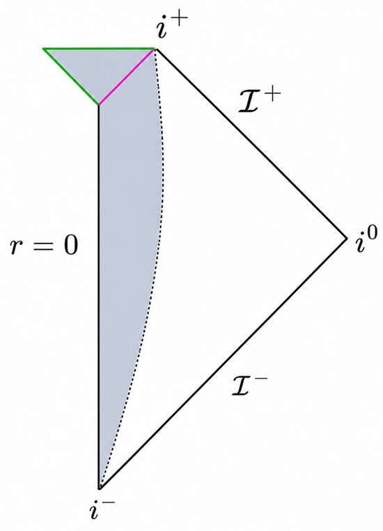
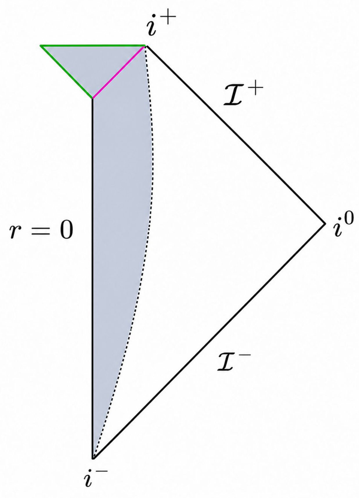
The results we obtained do not match those reported long ago [12,14,37,42]. It was found that the gravitational singularity that occurs during dust cloud collapse may be naked, so it might be seen by an external observer. The method used in these papers is based on the geometry of the neighbourhood of the gravitational singularity. This contradiction arises because the apparent horizon and the singularity form at the same instant in the inhomogeneous dust collapse, and in such cases, the tangent of the null geodesics and the tangent to the apparent horizon need to be investigated in the neighbourhood of the singularity. However, as we mentioned above, general relativity is unlikely to be applicable in that region. It is commonly expected that quantum gravity effects would be of primary importance there. The discussed dynamics of collapsing stars are presented in Figure 1.

Figure 1. Penrose diagram of an inhomogeneous pressureless cloud collapsing continually depicts the formation of the singularity and the apparent horizon: $r=0$ denotes the central shell of the collapsing cloud, $i^{\pm }$ are the future and past time-like infinitinites respectively, ${\mathcal{I}}^{\pm }$ are the future and past null infinities respectively, and $i^0$ denotes the space-like infinity. The shaded region denotes the collapsing LTB cloud, whose boundary is denoted by the dashed black line. This boundary is situated at a comoving radius $r_b$ and the non-shaded region denotes the Schwarzschild spacetime outside the collapsing star. The Israel–Darmois junction conditions ensure the smooth matching of the interior LTB spacetime with the exterior Schwarzschild spacetime at $r=r_b$, thereby completing the global conformal structure shown in the diagram. The green solid lines denote the singularity and the pink solid line denotes the apparent horizon. From this diagram, it becomes clear that at the time of formation, the singularity is not space-like; rather, it is parallel to ${\mathcal{I}}^{+}$, and hence it is null. As the collapse proceeds, the singularity becomes space-like, which is the case for a Schwarzschild singularity. This figure also shows that the time of formation of the singularity exactly coincides with the formation of the apparent horizon. In classical regime, this coincidence of the singularity and the apparent horizon formation enables null geodesics to escape. However, they are trapped within the apparent horizon instantly after, as can be clearly seen from this figure.

We plan to ascribe a quantum system to the gravitational model considered here using integral quantization [43,44,45,46,47,48,49,50,51,52]. Classical observables, such as expansion functions, would be represented by essentially self-adjoint operators acting in a suitable Hilbert space. Examination of the spectra of these operators would enable conclusions to be drawn concerning the trapped region in the context of quantum theory. For preliminary results addressing such an issue within effective loop quantum gravity, we recommend the recent paper by Fei et al. [53]. Such studies are beyond the scope of the present paper but will be carried out elsewhere.

References

- Hawking, S.W.; Ellis, G.F.R. The Large Scale Structure of Spacetime; Cambridge University Press: Cambridge, UK, 1973. [Google Scholar]
- Joshi, P.S. Global Aspects in Gravitation and Cosmology; Oxford University Press: Oxford, UK, 1993. [Google Scholar]
- Goswami, R.; Ellis, G.F.R. Almost Birkhoff Theorem in General Relativity. Gen. Relativ. Gravit. 2011, 43, 2157. [Google Scholar] [CrossRef] [Scilit]
- Oppenheimer, J.R.; Snyder, H. On continued gravitational contraction. Phys. Rev. 1939, 56, 455. [Google Scholar] [CrossRef] [Scilit]
- Datt, S. Über eine Klasse von Lösungen der Gravitationsgleichungen der Relativität. Z. Phys. 1938, 108, 314. [Google Scholar] [CrossRef] [Scilit]
- Tipler, F.J. Singularities in conformally flat spacetimes. Phys. Lett. 1977, 64A, 8. [Google Scholar] [CrossRef] [Scilit]
- Penrose, R. Gravitational Collapse: The Role of General Relativity. Riv. Nuovo C. Numero Spec. I 1969, 1, 252. [Google Scholar]
- Penrose, R. Singularities and Time-Asymmetry. In General Relativity: An Einstein Centenary Survey; Hawking, S.W., Israel, W., Eds.; Cambridge University Press: Cambridge, UK, 1979; pp. 581–638. [Google Scholar]
- Christodoulou, D. Violation of cosmic censorship in the gravitational collapse of a dust cloud. Commun. Math. Phys. 1984, 93, 171–195. [Google Scholar] [CrossRef] [Scilit]
- Newman, R.P.A.C. Strengths of naked singularities in Tolman-Bondi space-times. Class. Quantum Gravity 1986, 3, 527–539. [Google Scholar] [CrossRef] [Scilit]
- Newman, R.P.A.C.; Joshi, P.S. Constraints on the Structure of Naked Singularities in Classical General Relativity. Ann. Phys. 1988, 182, 112–119. [Google Scholar] [CrossRef] [Scilit]
- Joshi, P.S.; Dwivedi, I.H. Naked singularities in spherically symmetric inhomogeneous Tolman-Bondi dust cloud collapse. Phys. Rev. D 1993, 47, 5357. [Google Scholar] [CrossRef] [Scilit]
- Dwivedi, I.H.; Joshi, P.S. On the Occurrence of Naked Singularity in Spherically Symmetric Gravitational Collapse. Commun. Math. Phys. 1994, 166, 117. [Google Scholar] [CrossRef] [Scilit]
- Joshi, P.S.; Singh, T.P. Role of initial data in the gravitational collapse ef inhomogeneus dust. Phys. Rev. D 1995, 51, 6778. [Google Scholar] [CrossRef] [Scilit]
- Mosani, K.; Dey, D.; Joshi, P.S. Global visibility of a strong curvature singularity in nonmarginally bound dust collapse. Phys. Rev. D 2020, 102, 044037. [Google Scholar] [CrossRef] [Scilit]
- Madhav, T.A.; Goswami, R.; Joshi, P.S. Gravitational collapse in asymptotically anti-de Sitter/de Sitter backgrounds. Phys. Rev. D 2005, 72, 084029. [Google Scholar] [CrossRef] [Scilit]
- Goswami, R.; Joshi, P.S. Spherical gravitational collapse in N-dimensions. Phys. Rev. D 2007, 76, 084026. [Google Scholar] [CrossRef] [Scilit]
- Koushiki; Goswami, R.; Joshi, P.S. Universality and Criticality in Mass-less Scalar Field Collapse. arXiv 2025, arXiv:2512.20998. [Google Scholar] [CrossRef] [Scilit]
- Koushiki; Joshi, P.S. Apparent horizon and causal structure of spacetime singularities. arXiv 2025, arXiv:2508.14663. [Google Scholar] [CrossRef] [Scilit]
- Joshi, P.S.; Malafarina, D.; Narayan, R. Equilibrium configurations from gravitational collapse. Class. Quant. Grav. 2011, 28, 235018. [Google Scholar] [CrossRef] [Scilit]
- Joshi, P.S.; Malafarina, D.; Narayan, R. Distinguishing black holes from naked singularities through their accretion disc properties. Class. Quantum Gravity 2014, 31, 015002. [Google Scholar]
- Goswami, R.; Joshi, P.S. Gravitational collapse of a self-interacting scalar field. Mod. Phys. Lett. A 2007, 22, 65–74. [Google Scholar] [CrossRef] [Scilit]
- Mosani, K.; Dey, D.; Joshi, P.S. Globally visible singularity in an astrophysical setup. Mon. Not. Roy. Astron. Soc. 2021, 504, 4743–4750. [Google Scholar] [CrossRef] [Scilit]
- Mosani, K.; Koushiki; Joshi, P.S.; Trivedi, J.V.; Bhanja, T. Gravitational collapse of scalar and vector fields. Phys. Rev. D 2023, 108, 044049. [Google Scholar] [CrossRef] [Scilit]
- Koushiki; Joshi, P.S.; Bhattacharyya, S. On Formation of Primordial Naked Singularities. arXiv 2025, arXiv:2501.14695. [Google Scholar] [CrossRef] [Scilit]
- Akiyama, K. et al. [Event Horizon Telescope Collaboration]. First Sagittarius A* Event Horizon Telescope Results. I. The Shadow of the Supermassive Black Hole in the Center of the Milky Way. Astrophys. J. Lett. 2022, 930, L12. [Google Scholar] [CrossRef] [Scilit]
- Kluźniak, W.; Krajewski, T. Outflows from Naked Singularities, Infall through the Black Hole Horizon: Hydrodynamic Simulations of Accretion in the Reissner-Nordström Space-Time. Phys. Rev. Lett. 2024, 133, 241401. [Google Scholar] [CrossRef] [Scilit] [PubMed]
- Saurabh, S.; Bambhaniya, P.; Joshi, P.S. Imaging ultracompact objects with radiatively inefficient accretion flows. Astron. Astrophys. 2024, 682, A113. [Google Scholar] [CrossRef] [Scilit]
- Uniyal, A.; Dihingia, I.K.; Mizuno, Y.; Kluźniak, W. GRMHD Study of Accretion onto Time-like Naked Singularities. Astrophys. J. 2025, 993, 97. [Google Scholar] [CrossRef] [Scilit]
- Dey, D.; Shaikh, R.; Joshi, P.S. Shadow of nulllike and timelike naked singularities without photon spheres. Phys. Rev. D 2021, 103, 024015. [Google Scholar] [CrossRef] [Scilit]
- Joshi, A.B.; Dey, D.; Joshi, P.S.; Bambhaniya, P. Shadow of a Naked Singularity without Photon Sphere. Phys. Rev. D 2020, 102, 024022. [Google Scholar] [CrossRef] [Scilit]
- Solanki, D.N.; Bambhaniya, P.; Dey, D.; Joshi, P.S.; Pathak, K.N. Shadows and precession of orbits in rotating Janis–Newman–Winicour spacetime. Eur. Phys. J. C 2022, 82, 77. [Google Scholar] [CrossRef] [Scilit]
- Dey, D.; Shaikh, R.; Joshi, P.S. Perihelion precession and shadows near black holes and naked singularities. Phys. Rev. D 2020, 102, 044042. [Google Scholar] [CrossRef] [Scilit]
- Góźdź, A.; Ostrowski, J.J.; Pȩdrak, A.; Piechocki, W. Quantum system ascribed to the Oppenheimer–Snyder model of massive stars. Eur. Phys. J. C 2024, 84, 10. [Google Scholar] [CrossRef] [Scilit]
- Schmitz, T. Towards a quantum Oppenheimer-Snyder model. Phys. Rev. D 2020, 101, 026016. [Google Scholar] [CrossRef] [Scilit]
- Goswami, R.; Joshi, P.S.; Singh, P. Quantum evaporation of a naked singularity. Phys. Rev. Lett. 2006, 96, 031302. [Google Scholar] [CrossRef] [Scilit] [PubMed]
- Barve, S.; Singh, T.P.; Vaz, C.; Witten, L. A simple derivation of the naked singularity in spherical dust collapse. Class. Quantum Gravity 1999, 16, 1727. [Google Scholar] [CrossRef] [Scilit]
- Booth, I.; Heller, M.P.; Plewa, G.; Spalinski, M. On the apparent horizon in fluid-gravity duality. Phys. Rev. D 2011, 83, 106005. [Google Scholar] [CrossRef] [Scilit]
- Ashtekar, A.; Krishnan, B. Dynamical horizons and their properties. Phys. Rev. D 2003, 68, 104030. [Google Scholar] [CrossRef] [Scilit]
- Schnetter, E.; Krishnan, B.; Beyer, F. Introduction to dynamical horizons in numerical relativity. Phys. Rev. D 2006, 74, 024028. [Google Scholar] [CrossRef] [Scilit]
- Poisson, E. A Relativist’s Toolkit: The Mathematics of Black-Hole Mechanics; Cambridge University Press: Cambridge, UK, 2009; p. 12. [Google Scholar]
- Joshi, P.S.; Dadhich, N.; Maartens, R. Why do naked singularities form in gravitational collapse? Phys. Rev. D 2002, 65, 101501. [Google Scholar] [CrossRef] [Scilit]
- Gazeau, J.-P.; Piechocki, W. Coherent state quantization of a particle in de Sitter space. J. Phys. A Math. Gen. 2004, 37, 6977. [Google Scholar] [CrossRef] [Scilit]
- Bergeron, H.; Czuchry, E.; Gazeau, J.-P.; Małkiewicz, P.; Piechocki, W. Smooth Quantum Dynamics of Mixmaster Universe. Phys. Rev. D 2015, 92, 061302. [Google Scholar] [CrossRef] [Scilit]
- Bergeron, H.; Czuchry, E.; Gazeau, J.-P.; Małkiewicz, P.; Piechocki, W. Singularity avoidance in a quantum model of the Mixmaster universe. Phys. Rev. D 2015, 92, 124018. [Google Scholar] [CrossRef] [Scilit]
- Góźdź, A.; Kisielowski, M.; Piechocki, W. Quantum dynamics of gravitational massive shell. Phys. Rev. D 2023, 107, 046019. [Google Scholar] [CrossRef] [Scilit]
- Piechocki, W.; Schmitz, T. Quantum Oppenheimer-Snyder model. Phys. Rev. D 2020, 102, 046004. [Google Scholar] [CrossRef] [Scilit]
- Góźdź, A.; Pȩdrak, A.; Piechocki, W. Ascribing quantum system to Schwarzschild spacetime with naked singularity. Class. Quantum Gravity 2022, 39, 145005. [Google Scholar] [CrossRef] [Scilit]
- Góźdź, A.; Pȩdrak, A.; Piechocki, W. Quantum system ascribed to the Oppenheimer-Snyder model of massive stars. Eur. Phys. J. C 2024, 83, 150. [Google Scholar]
- Góźdź, A.; Piechocki, W.; Plewa, G. Quantum Belinski-Khalatnikov-Lifshitz scenario. Eur. Phys. J. C 2019, 79, 45. [Google Scholar] [CrossRef] [Scilit]
- Góźdź, A.; Piechocki, W. Robustnes of the BKL scenario. Eur. Phys. J. C 2020, 80, 142. [Google Scholar] [CrossRef] [Scilit]
- Góźdź, A.; Pȩdrak, A.; Piechocki, W. Quantum dynamics corresponding to the chaotic BKL scenario. Eur. Phys. J. C 2023, 83, 150. [Google Scholar] [CrossRef] [Scilit]
- Fei, X.; Long, G.; Ma, Y.; Zhang, C. Expansion operators in spherically symmetric loop quantum gravity. arXiv 2026, arXiv:2602.15628. [Google Scholar] [CrossRef] [Scilit]
Disclaimer/Publisher’s Note: The statements, opinions and data contained in all publications are solely those of the individual author(s) and contributor(s) and not of MDPI and/or the editor(s). MDPI and/or the editor(s) disclaim responsibility for any injury to people or property resulting from any ideas, methods, instructions or products referred to in the content. |
© 2026 by the authors. Licensee MDPI, Basel, Switzerland. This article is an open access article distributed under the terms and conditions of the Creative Commons Attribution (CC BY) license.