


Abstract
When high-energy particles of cosmic origin penetrate the atmosphere, they collide with atmospheric atoms and molecules, triggering cascades of secondary particles that can propagate down to the surface. These energetic particles constitute a radiation background in the atmosphere with direct implications for aviation exposure safety and influence atmospheric chemistry through the ionization of ambient air. For these reasons, the development of secondary particle showers has been extensively studied, and considerable effort has been devoted to Monte Carlo-based models capable of computing secondary particle fluxes in the atmosphere. However, the atmospheric models in which particle transport is simulated are generally standard atmospheric models, which can differ substantially from actual atmospheric conditions. In this work, the Atmospheric Radiation Interaction Simulator (AtRIS) is used in conjunction with the NRLMSIS-2.1 atmospheric model to investigate the effects of varying density, pressure, and temperature profiles on secondary particle fluxes at different atmospheric levels. For a given incident radiation spectrum, the AtRIS simulations reveal substantial differences between atmospheric profiles when a uniform vertical cutoff rigidity is prescribed across all latitudes, effectively isolating atmospheric effects from geomagnetic shielding. Below ∼20 km, secondary particle fluxes are consistently higher in the polar atmosphere than at the equator. At ∼7 km, the difference between the equatorial and southern polar winter profiles reaches ∼40% for protons, photons, electrons, and positrons, and ∼30% for neutrons and muons.
1. Introduction
The Earth’s atmosphere is continuously bombarded by particles originating from space, whose nature, energy, and abundance vary significantly depending on their sources. The most energetic of these particles are Galactic Cosmic Rays (GCRs), which have been thought to be accelerated by diffusive shock acceleration in the shock front of Supernova remnants (SNRs) [1]. However, the maximum energy of particles in SNRs is limited and discrepancies between observations and these expectations from SNRs have been reported [2]. New sources of very high energy GCRs are currently investigated, such as star clusters [3] and micro quasars [4]. GCRs are primarily composed of protons and alpha particles; while the bulk of the Galactic component is typically quoted over the range ∼ eV/nucleon to ∼ eV/nucleon [5], Voyager 1 has directly measured the GCR flux down to a few MeV/nucleon in the local interstellar medium [6], below which solar modulation and, closer to Earth, contributions from solar energetic particles increasingly dominate the locally observed spectrum. They form a persistent background source of particles that penetrate the atmosphere. As GCRs propagate through the solar system, they interact with the solar wind, leading to periodic variations in their flux that correlate with the solar cycle. Depending on solar activity, the peak of the GCRs spectrum measured at Earth shifts between ∼200 MeV/nucleon and ∼600 GeV/nucleon [7].
Energetic particles interact with the atoms and molecules in the atmosphere. When their energy is sufficiently high (∼1 GeV/nucleon for protons and alpha particles), the precipitating particles can initiate an atmospheric particle cascade (APC). In this work, we distinguish the APC from extensive air showers (EASs), which share a similar origin but are triggered by much higher energy particles (∼ eV) [8]. APC consists of three main components: the electromagnetic cascade, the muonic cascade, and the hadronic cascade [9]. As the altitude decreases, the number of particles in the APC increases exponentially until it reaches a critical energy threshold, below which it can no longer produce additional particles. At this point, ionization of the ambient air becomes the dominant process through which secondary particles lose their energy, causing the cascade to diminish rapidly [10]. In this context, the precipitating Galactic Cosmic Rays (GCRs) are often referred to as Primary Cosmic Rays (PCRs), while the particles produced in the cascade are termed Secondary Cosmic Rays (SCRs).
The propagation of PCRs and SCRs through the atmosphere has significant implications across multiple domains of physics. For example, cosmogenic radionuclides such as 14C, which are widely used in carbon dating, are produced through collisions involving cosmic rays [11]. Additionally, precipitating radiation from space influences the chemistry of the upper atmosphere, particularly in the mesosphere and upper thermosphere, through direct ionization [12,13]. Energetic particles also represent the primary source of natural radiation exposure at commercial flight altitudes and above [14,15]. Furthermore, SCRs can induce soft errors in semiconductors, posing risks to electronic systems [16].
Currently, the most accurate models for simulating APC are based on Monte Carlo particle transport codes, such as GEANT4 [17], MCNP [18], CORSIKA [19], and FLUKA [20]. Additionally, dedicated toolkits have been developed using these transport codes to simulate APC and their effects in planetary atmospheres, enabling the computation of SCR fluxes, ionization rates, and dose rates [21,22,23,24,25,26]. However, running these models for a full spectrum of PCRs is computationally expensive and time-consuming. To address this challenge, fast-running analytical models have been developed, which use parametrizations of full APC simulations [27,28].
In addition to the nuclear transport code, an essential component in simulating APC is the target material through which the particles propagate. For planetary bodies, these targets are their atmospheres and/or crusts. For Earth-based dosimetric and ionization-rate applications, most simulation toolkits use standard atmospheric models to compute density, pressure, and temperature profiles. In many cases, standard atmospheric models such as the US Standard Atmosphere [29] or the International Standard Atmosphere [30] are employed in APC simulations. However, atmospheric properties vary continuously in both time and space, which standard models cannot fully capture. Variations in atmospheric parameters have been shown to impact APC development, ranging from ∼2% diurnal variations to ∼10% seasonal variations [31,32]. Recently, a study [33] computed muon fluxes using MCNP6 and atmospheric temperature and pressure profiles measured over Brussels. Their findings revealed a complex correlation between temperature and muon flux in the first 20 km of the atmosphere. Nevertheless, the use of realistic atmospheric parameters in practical APC simulations remains limited, and the use of standard atmospheric profiles is still common in dosimetric and ionization-rate applications. In contrast, EAS reconstruction at the Pierre Auger Observatory and the Telescope Array relies on advanced atmospheric monitoring systems (molecular and/or aerosol) that provide accurate, site-specific atmospheric conditions [34,35]. In this work, we use the Atmospheric Radiation Interaction Simulator (AtRIS [36]) and the NRLMSIS-2.1 atmospheric model [37,38] to investigate the impact of varying atmospheric parameter profiles on the fluxes of SCR.
This work is organized as follows: In Section 2, we begin with a brief introduction of AtRIS (Section 2.1), followed by a description of the method used to compute the secondary cosmic ray spectra (Section 2.2). In Section 3.1, we assess the associated spreads and validate the results using PARAM/EXPACS (Section 3.2). Then we investigate the differences in SCR fluxes resulting from simulations set up with different atmospheric profiles (Section 3.3). Finally, we discuss and conclude our findings in Section 4.
2. Methods and Data
2.1. The Atmospheric Radiation Interaction Simulator (AtRIS)
The Atmospheric Radiation Interaction Simulator (AtRIS) is a toolkit designed to simulate the propagation of energetic particles through planetary atmospheres. AtRIS is based on GEANT4, a Monte Carlo toolkit developed at CERN (https://home.cern/) for simulating particle transport through matter [17].
AtRIS enables the computation of ionization rates together with absorbed and equivalent dose rates induced in planetary atmospheres by cosmic radiation. Its modular design offers users significant flexibility in specifying both the planet and the atmosphere under investigation, making it suitable not only for terrestrial applications but also exoplanetary studies [39]. AtRIS has been validated for Earth [36,40] using the NRLMSISE-00 model [41], as well as for Mars [42] and Venus [43].
While AtRIS directly provides ionization and dose rates, the computation of secondary particle fluxes at different atmospheric altitudes requires additional post-processing by the user. AtRIS makes it possible to access the secondary particle data generated throughout the atmospheric cascade and thereby derive the corresponding fluxes.
2.2. Secondary Particle Computation
To compute secondary particle fluxes in the atmosphere, we followed the step-by-step procedure outlined in [42]. This procedure converts the binary data output by AtRIS into two-dimensional histograms, linking the energy of primary particles to that of secondary particles. Such a histogram, denoted as , can be constructed for a specific type of primary particle p, a specific type of secondary particle s, and a given altitude h. Using , we can then derive additional histograms or matrices to calculate the fluxes and spectra of secondary particles in the atmosphere.
2.2.1. Secondary Atmospheric Response Matrix (SARM)
We define the Secondary Atmospheric Response Matrix (SARM), denoted as , in such a way that, given a type of secondary particle and the total flux of primary GCRs, the flux of secondary particle as a function of altitude can be expressed as:
where is the total flux (in []) of primary particle of type p with energy precipitating into the atmosphere. And the SARM can be written as:
where is the number of primary particles simulated in the energy bin whose center is . is the area of the spherical shell at altitude h, with being the radius of the Earth. is a geometric factor corresponding to the integration of the cosine of the zenith angle of secondaries crossing the surface plane. In this case, we consider both downward and upward propagating secondaries, so .
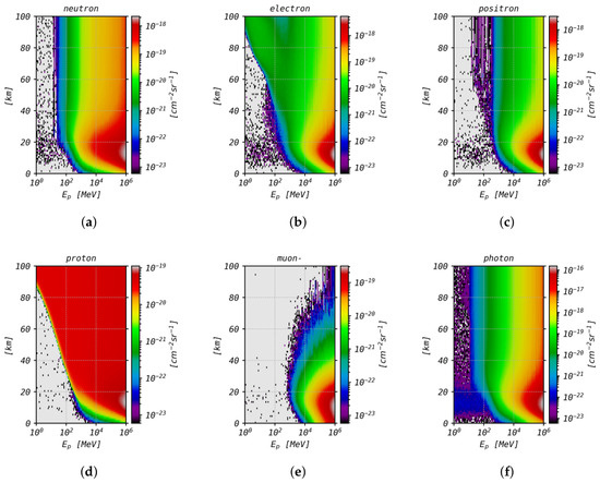
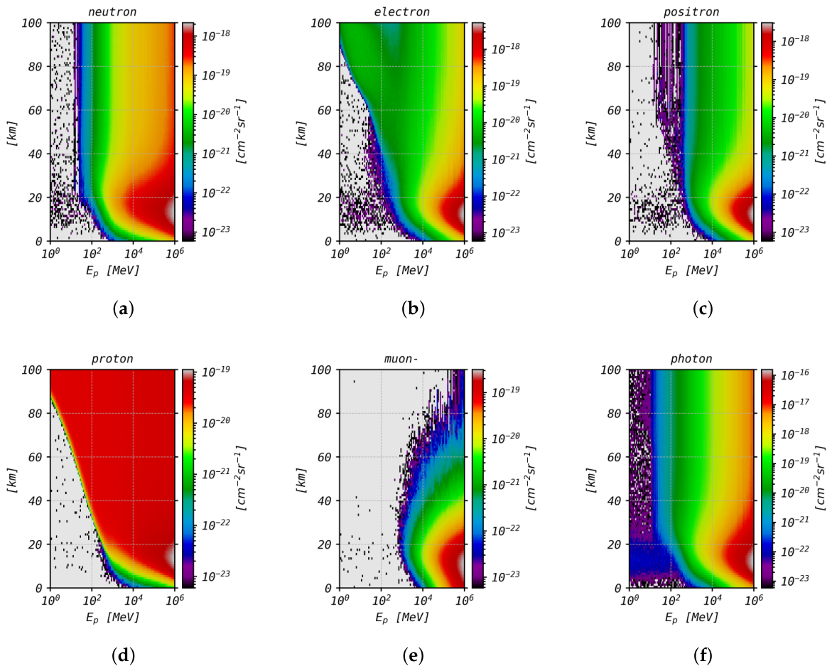
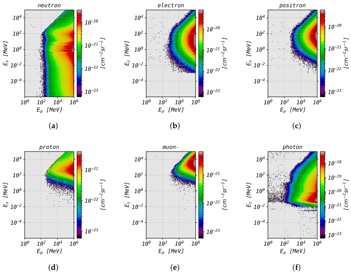
The SARM characterizes the relationship between primary particle energy and the average altitude-dependent production of secondary particles. It is analogous to the atmospheric response matrices described in [36,40] for ionization and dose rates. However, the SARM does not provide information about the energy distribution of secondary particles. SARMs for different particle types are presented in Figure 1.
Figure 1.
The Secondary Atmospheric Response Matrices (SARM) describing the relation between primary particle energy and the resulting average altitude-dependent secondary particle production. Each panel corresponds to the SARM of a specific secondary particle. (a) Neutrons; (b) electrons; (c) positrons; (d) protons; (e) muons-; (f) photons.
2.2.2. Secondary Spectrum Response Matrix (SSRM)
The Secondary Spectrum Response Matrix (SSRM) is defined at a fixed altitude as follows:
The SSRM is similar to the SARM, but it describes the relationship between the primary particle energy and the resulting secondary particle energy rather than the altitude at which they are produced. This means that the SSRM must be recomputed for each altitude. The SSRM can then be used to compute different spectra of secondary particles,
where is the differential spectrum in [],
where is the integral spectrum in [],
where is the lethargy spectrum in [], and in the width of the energy bin.
The total flux of primary particles precipitating into the atmosphere, , can be computed from the GCRs differential spectrum, denoted , as follows:
where is the width of the primary particle energy bins, is the area of the spherical shell corresponding to the top of the atmosphere. is the integration of the cosine of the zenith angle of the source particles. In this case, because they were injected isotropically inward from the source sphere, .
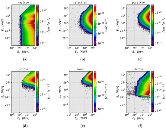
Example of SSRM computed for different secondary particles at 15 km is shown in Figure 2.
Figure 2.
Secondary Spectrum Response Matrices (SSRMs) describing the relationship between primary particle energy and the resulting secondary particle energy. Each panel represents the SSRM for a specific secondary particle at an altitude of 15 km. (a) Neutrons; (b) electrons; (c) positrons; (d) protons; (e) muons-; (f) photons.
2.2.3. Primary Galactic Cosmic Ray Spectrum
To obtain a realistic and meaningful flux of secondary particles, it is also essential to compute a realistic flux of primary GCRs entering the atmosphere. As GCRs propagate through the heliosphere, they interact with the magnetized plasma of the solar wind. The modulation of GCRs in the heliosphere is governed by the Parker transport equation [44]. In this work, we use the force-field approximation (FFA) to calculate the modulated GCRs flux at 1 AU [45]. Within this framework, the modulated differential flux can be expressed as:
denotes the Local Interstellar Spectrum (LIS) of the primary particle (i.e., the differential spectrum outside the heliosphere). is the rest energy of the primary particle, and represents the solar modulation function, given by . Z and A are the charge and mass number of the primary particle, respectively. The modulation potential, , is the only free parameter in this approximation and serves as a direct measure of solar activity. It can be determined using satellite measurements (e.g., PAMELA and BESS) or ground-based neutron monitor and muon detector count rates [46,47,48,49,50]. As shown in Equation (8), the differential spectrum of GCRs depends on the choice of the LIS. In this work, we adopt the LIS parametrization proposed by [51], which incorporates Voyager 1 observations from outside the heliosphere. This parametrization significantly improves the prediction of GCRs proton fluxes at energies below 500 MeV. Note that at those energy levels, primary particles do not have sufficient energy to trigger full APC; however, they can produce electromagnetic cascades from pion decay () limited at high altitude.
3. Results
3.1. Statistical Spread
Most transport models, including AtRIS, do not provide formal estimates of uncertainty for particle fluxes, ionization rates, or dose rates. To address this limitation, we quantified the statistical spread of AtRIS for secondary particle fluxes at various altitudes. This spread arises both from the intrinsic stochasticity of particle transport at low energy and from uncertainties in the underlying physics models used by AtRIS/Geant4 in this regime. Our uncertainty estimate was derived by running AtRIS multiple times under identical conditions, using protons with energies between 1 MeV and 1 TeV. Each of the repeated runs was launched with an independent random seed, ensuring that the resulting spread reflects genuine Monte Carlo sampling variance rather than repeated identical simulations. The energy range was divided into 120 bins, uniformly distributed in logarithmic space. In each simulation, approximately 5000 protons were sampled per energy bin. The FTFP_BERT_HP physics list is used for all runs.
Given that a single simulation and data processing with this setup requires, on average, 27 h on a Linux-based workstation equipped with 104 Intel Xeon Gold 5320 CPU cores operating at 2.20 GHz, we repeated the process ten times (cumulatively totaling 11.3 days). To estimate the uncertainty, we analyzed multiple metrics, including the standard deviation (), the standard error of the mean (), and the 95% confidence interval derived from a t-distribution ().
For all estimates, the uncertainty in secondary particle flux depends on the type of secondary particle, its energy, and its altitude. However, the magnitude of these uncertainties varies significantly. Given the limited number of simulations available for error estimation, we adopted a conservative approach by using the confidence interval as the worst-case scenario. Under the Gaussian assumption, this choice ensures that approximately 99% of the simulated flux values lie within the reported error bounds. Hereafter, we refer to the interval as the standard spread. We acknowledge that in bins where the reported spread exceeds %, the symmetric interval is a poor approximation, since it can extend to unphysical (negative) flux values. This indicates that the underlying distribution of simulated flux values is not well described by a Gaussian in these bins, and the reported percentage should be interpreted as an order-of-magnitude indicator of high run-to-run variability rather than a strict confidence interval in these regions.
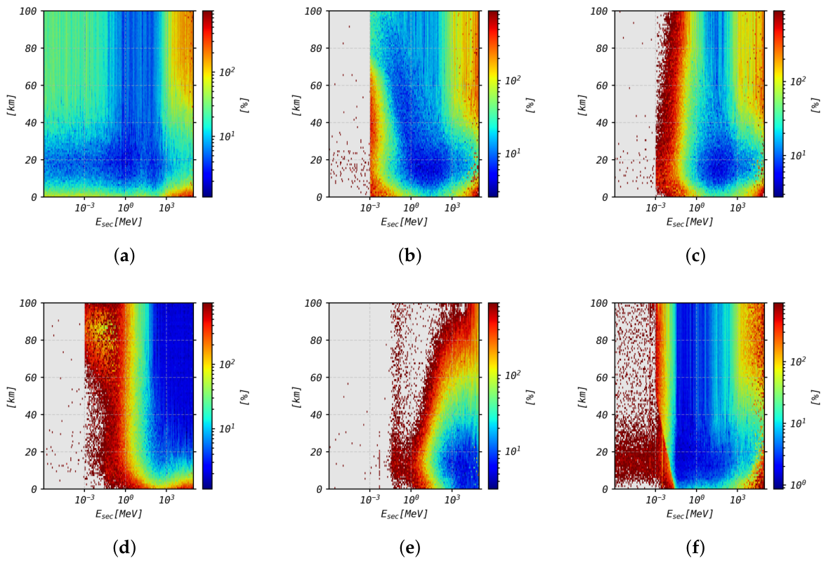
The standard spread of the differential spectra for various secondary particle types at different altitudes are presented in Figure 3. Across all panels (i.e., for all secondary particles), the spread varies dramatically, ranging from ∼3% to ∼500%. The altitude and energy ranges at which the spread is minimized differ for each secondary particle type.
- Neutrons exhibit the smallest overall spread. The spread remains below 25% in an altitude band from ∼5 km to ∼35 km across all energies. However, for energies above ∼103 MeV, the spread increases rapidly above ∼40 km and below ∼5 km.
- For electrons, the energy range in which the spread remains below 25% shifts to higher energies as altitude decreases, down to ∼20 km. Below 10 km, the spread exceeds 100% in the energy ranges of – MeV and – MeV.
- The spread on positron flux closely resembles that of electrons, except above 70 km, where the spread exceeds 100% in the lower energy range (– MeV).
- For protons, the spread is below 25% only at energies above ∼10 MeV and altitudes above 10 km. At lower energies, the spread quickly exceeds 100%.
- Muons differ from other particles, exhibiting the smallest spread at the highest energies near the surface. The spread exceeds 25% at altitudes above 40 km and energies below 100 MeV.
- Photons in the energy range of – MeV show spreads below 25% at all altitudes. Similar to neutrons, the spread for photon flux is also smaller at higher energies within an altitude band of ∼5 km to ∼40 km.
Figure 3.
The standard spread (3) relative to the mean in percent for each secondary particle as a function of energy and altitude. The color bar is in logarithmic scale. (a) Neutrons; (b) electrons; (c) positrons; (d) protons; (e) muons-; (f) photons.
3.2. Validation: Comparison Between AtRIS and PARAM/EXPACS
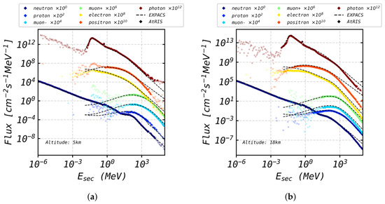
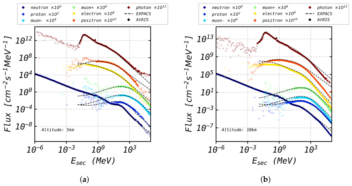
As previously noted, the secondary particle fluxes derived from AtRIS have been validated against observations on Earth and Mars. However, for Earth, only muon and neutron fluxes were reported [36]. In the present study, we compare the differential spectra of secondary particles computed with AtRIS to those from the PARAM/EXPACS analytical model (version 3 [27]). This model employs analytical functions fitted to validated APC simulations generated using the Particle and Heavy Ion Transport code System (PHITS [52]). Figure 4 displays the differential spectra of various secondary particles, as computed by AtRIS and PARAM/EXPACS, at altitudes of 5 km (panel a) and 18 km (panel b). For AtRIS, the portions of the spectra where the spread exceeds 50% were displayed with increased transparency. Note that, for each particle type, the differential spectra shown in the figure are scaled by a constant factor (a multiple of 100). This scaling was applied to visually separate the curves and improve readability. The exact scaling factor for each curve is explicitly indicated in the legend.
Figure 4.
Differential spectra of various secondary particles computed with AtRIS (colored diamonds) and PARAM/EXPACS (black dashed lines) at different altitudes. Each color corresponds to a given type of particle. The differential spectra are scaled by a constant factor given in the legend of the panels. Semi-transparent points correspond to the results from AtRIS where the spread is larger than 50%. (a) Altitude: 5 km; (b) Altitude: 18 km.
A vertical cutoff rigidity of GV is assumed in both AtRIS and PARAM/EXPACS. Overall, they show good agreement for all simulated particles, particularly for neutrons and protons. However, above ∼1 GeV, both models begin to diverge significantly. The discrepancy increases with the energy of the secondary particles, notably for photons, electrons and positrons at 5 km, and for all particles at 18 km. As altitude increases, so do the differences between the models at high energies. In this higher energy range, PARAM/EXPACS systematically predicts larger fluxes than AtRIS, except for photons above 1 GeV, where the AtRIS spectra are slightly higher.
The greatest discrepancy between the models occurs for positrons. At 18 km, the difference reaches three orders of magnitude at 100 GeV. This substantial discrepancy is partly attributable to the parametrization used in PARAM. Ref. [27] demonstrated that, above 1 GeV, the positron parametrization begins to overestimate the results obtained from PHITS. While similar overestimations occur for electrons and photons, they are less pronounced.
3.3. Atmospheric Profiles
3.3.1. Atmospheric Density Profiles
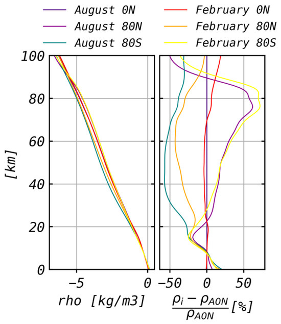
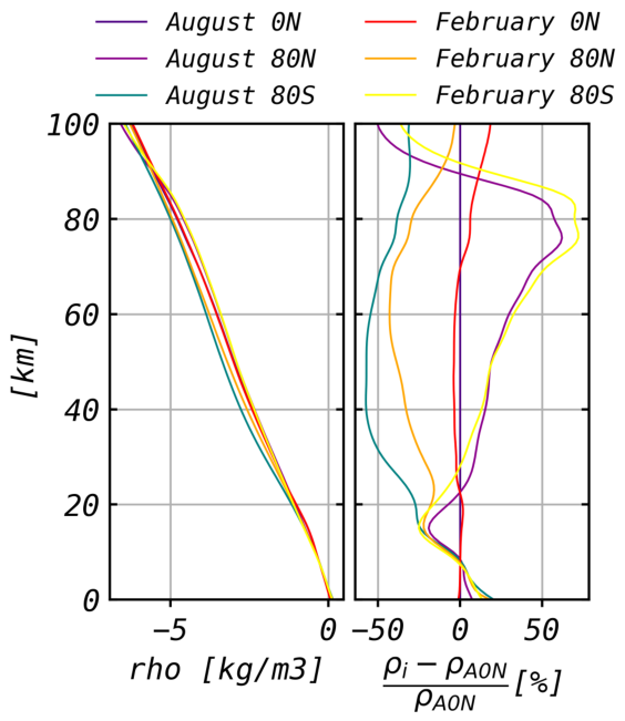
In this section, we investigate the impact of the atmospheric model on secondary particle fluxes. Using the NRLMSISE-2.1 model, we computed atmospheric density, temperature, and composition profiles under varying conditions. Six distinct profiles were generated to capture latitudinal and seasonal effects: August at 80° North (A80N), August at 0° North (A0N), August at 80° South (A80S), February at 80° North (F80N), February at 0° North (F0N), and February at 80° South (F80S). All profiles were calculated at noon, with a longitude of 0°. The resulting vertical density profiles are presented in Figure 5 (left panel).
Figure 5.
The left panel displays the vertical density profiles computed with NRLMSISE-2.1 for various latitudes and dates. The right panel shows the relative differences between those profiles. In this case, the reference profile is the one computed at the equator in August (i.e., A0N).
Since the atmosphere is in hydrostatic equilibrium, the variation in density with altitude follows a similar pattern across all profiles. However, changes in latitude or season do affect the density profiles. The right panel of Figure 5 illustrates the relative difference between these profiles, using the August equatorial density profile (A0N) as a reference.
As would be expected, the difference between the two equatorial density profiles (A0N and F0N) remains minimal at most altitudes, below 5% up to 75 km and below 10% up to 90 km. In contrast, the relative differences with the high-latitude profiles exhibit significant variability with altitude. As shown in the right panel of the figure, the local winter (F80N, A80S) and local summer (F80S, A80N) profiles diverge distinctly above 20 km. During local winter, the atmospheric density above 10 km is consistently lower than at the equator. This effect is most pronounced in the southern hemisphere winter, where the relative difference reaches −57% at 40 km. For the northern hemisphere winter, the maximum relative difference occurs at 60 km, reaching −40%.
In contrast to the local winter profiles, the density during local summer exceeds that of the equator between 25 km and 90 km. Both summer profiles (F80N and A80S) remain close to each other, generally within 5–10%. The largest deviations relative to the equatorial density occur at approximately 80 km, reaching about 60–70%.
Finally, below 18 km, all high-latitude density profiles converge. Between 8 km and 18 km, the density at high latitudes is lower than at the equator. Below 8 km, however, the density at high latitudes becomes greater than at low latitudes.
3.3.2. Effect of Atmospheric Densities on Secondary Particle Flux Profiles
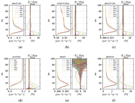
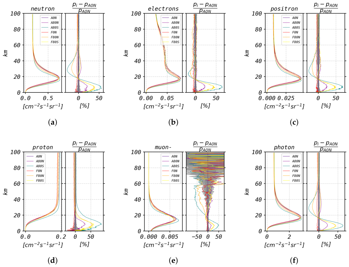
Using AtRIS, we computed the SCR fluxes for each of the aforementioned atmospheric density profiles, while accounting for variations in both temperature and composition. In this case, the atmosphere is divided into 200 layers, from the ground up to 100 km. The layers have a non-uniform vertical resolution. Their thickness is 0.25 km from 0 km–25 km, 0.5 km from 25 km–50 km and 1 km from 50 km to 100 km. All six simulations employed the FTFP_BERT_HP physics list [53]. The energy of the PCRs spans from 1 MeV to 1 TeV, divided into 120 bins uniformly distributed in logarithmic space. The results are presented in Figure 6, where each panel corresponds to a specific type of secondary particle. Each panel displays both the vertical profile of the particle’s integral flux (in ) and the relative difference between the August equatorial profile and the other profiles, analogous to the density profiles discussed earlier.
Figure 6.
Each panel shows the vertical profiles of secondary particle flux () and the relative difference (%) between the August equatorial profile and the other profiles. In the relative difference panel (right), the grayed areas correspond to 1, 2 and 3 (in percent). (a) Neutrons; (b) electrons; (c) positrons; (d) protons; (e) muons-; (f) photons.
The PCRs flux is identical across all six simulations. We adopt solar minimum conditions ( MV) and, to isolate the influence of atmospheric parameters on the SCRs, we deliberately neglect geomagnetic shielding by setting the vertical cutoff rigidity to zero, even for equatorial profiles.
All flux profiles, except for protons, exhibit a maximum at approximately 18 km. This maximum occurs at the altitude where the production and loss of secondary particles reach equilibrium. Above this altitude, the particle cascade is not yet fully developed, whereas below it, decay processes and loss mechanisms dominate. For protons, no such maximum is observed because the flux profiles also include primary protons. Consequently, the vertical proton flux profile can be divided into two distinct regions. Above 30 km, the flux remains dominated by the primary Galactic Cosmic Ray flux precipitating into the atmosphere. Below 30 km, the flux is primarily composed of secondary protons generated within the particle cascade.
While the flux profile of each secondary species retains a similar shape when atmospheric properties are altered in the simulation, notable differences emerge among the profiles. For example, the profile computed for the southern high latitude in winter (A80S) deviates the most from the others. When a secondary particle exhibits a flux maximum, the A80S peak is consistently located approximately 2–3 km lower than in the other profiles. Additionally, for muons and neutrons, the A80S profile systematically yields the highest maximum flux among all profiles.
The relative differences between the August equatorial flux profile (A0N) and the other profiles highlight their discrepancies. Among these, the relative difference between the two equatorial profiles (A0N and F0N) is the smallest across all particle types. Indeed, the seasonal variability in atmospheric structure is comparatively weak relative to high latitudes. As a result, the atmospheric density, temperature, and composition profiles in A0N and F0N remain relatively similar, leading to only minor differences in the production and transport of secondary particles. All relative difference profiles for high-latitude regions exhibit a double-peak structure, except for protons. For protons, only a single positive peak appears at ∼20 km in the relative difference profiles, indicating that the flux of secondary protons is higher at high latitudes than near the equator. For other particles, this peak is also present, but they additionally feature a second peak above ∼20 km, whose sign depends on the season. During local winter (A80S and F80N), this second peak is negative, reflecting a higher flux of secondary particles in equatorial regions. Conversely, during local summer, the peak is positive, indicating greater flux at high latitudes.
Furthermore, the magnitude of the differences between the profiles above 20 km indicates that the reduction in secondary particle flux at high latitudes during winter, compared to the equator, is significantly greater than the increase observed in summer. This effect is particularly pronounced for muons. The maximum values of the relative difference between equatorial and high-latitude secondary particle fluxes below 20 km are presented in Table 1. The table reveals that, for all simulated particles, the largest differences between the equatorial and other profiles occur during the local winter in the southern hemisphere. This corresponds to the density profile that deviates most from the equatorial densities. Conversely, the smallest differences are observed between the equator and the northern hemisphere summer, a trend also reflected in the density differences between these profiles.
Table 1.
Maximum relative difference between the equatorial and high-latitude secondary particle flux profiles below 20 km, with the associated statistical spread (in percentage) given for each value.
To verify that these results are not driven by the noisiest bins identified in Figure 3, we recomputed the maximum relative differences reported in Table 1 restricting the analysis to altitude-energy bins where the statistical spread is below 30%. We find no significant change in the reported values, confirming that the differences between atmospheric profiles are not artifacts of the noisiest, least-constrained bins.
Moreover, to assess whether the atmospheric-density-driven differences reported above are robust to geomagnetic shielding, we repeated the comparison between the equatorial (A0N) and southern polar winter (A80S) profiles under a common vertical cutoff rigidity, applied identically to both profiles and swept from Rc = 0 to Rc = 20 GV (Table 2). For all species, the maximum relative difference below 20 km decreases as Rc increases, but remains well above the associated statistical spread at every cutoff value tested. Protons are the most sensitive species, with the maximum difference decreasing from 80% at Rc = 0 GV to 50% at Rc = 20 GV, a reduction of 30 percent, markedly larger than for any other secondary species (9–15%, Table 2). This is expected, since protons are also the primary particle type in our simulations: raising the cutoff directly removes low-energy primary protons, affecting both the primary and secondary proton populations simultaneously, whereas the other species are only indirectly affected through the resulting change in the secondary particle cascade. These results confirm that the atmospheric-density effect is not an artifact of the unrealistic abundance of low-energy primaries admitted at Rc = 0, but persists across the full range of cutoff conditions tested. We note, however, that this test applies a common cutoff to both profiles and does not reproduce the fully realistic, asymmetric configuration in which the equator (Rc ≈ 15 GV) and poles (Rc ≈ 0 GV) experience markedly different shielding simultaneously.
Table 2.
Maximum relative difference between the equatorial (A0N) and winter polar southern (A80S) secondary particle flux profiles below 20 km for different values of Rc.
3.3.3. Effect of Atmospheric Densities on Secondary Particle Spectra
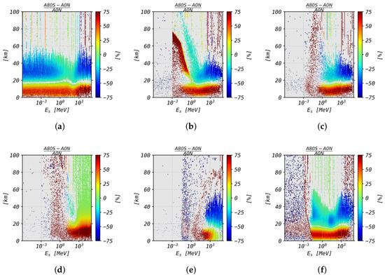
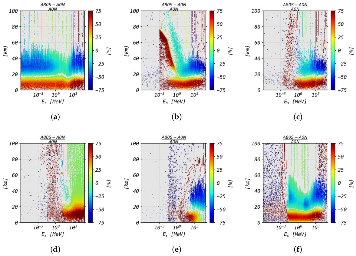
In addition to examining the impact of atmospheric densities on secondary particle flux, we also investigated their effects on secondary particle spectra. Figure 7 presents the results of the comparison between the southern winter (A80S) and equatorial (A0N) secondary particle spectra. Each panel illustrates the relative difference between the A0N and A80S differential spectra across all altitudes for a specific particle type. The shaded areas indicate the energy and altitude ranges where the model spread exceeds the relative differences.
Figure 7.
Relative difference between the August equatorial and the August high latitude secondary differential spectrum for each secondary particle as a function of energy and altitude. (left) Relative difference between the equatorial and the high northern latitude spectra. (right) Relative difference between the equatorial and the high southern latitude spectra. (a) Neutrons; (b) electrons; (c) positrons; (d) protons; (e) muons-; (f) photons.
The panels in this figure align with the relative differences observed between the southern winter and equatorial profiles. Above 20 km, the relative difference is predominantly negative, while it becomes positive below this altitude. However, the panels also clearly demonstrate that the spectral differences are not uniform across all energies.
The differential spectra of secondary particles, when comparing equatorial and high-latitude atmospheric density profiles, can differ by up to 100% at altitudes above 20 km.
For all particles at altitudes below 20 km, except for muons, the relative differences between the southern winter high-latitude and equatorial spectra tend to increase with the energy of the secondary particles. For muons, however, the relative difference in the spectrum below 15 km increases as the energy decreases.
For neutrons, the relative difference between the two spectra above 20 km is consistently negative. At a fixed altitude, the relative differences reach a maximum (∼40%) below ∼1 MeV and above ∼500 MeV. Between these energies, the relative difference in the neutron spectra exhibits a clear minimum centered around ∼50 MeV.
The relative differences between the photon differential spectra follow a similar pattern to that of neutrons. However, above 20 km, the relative differences for photons feature three maxima, compared to two for neutrons.
For muons, the relative differences above 30 km are more uniform across energies, while between 15 km and 30 km, the relative difference between A0N and A80S increases with energy.
For protons, between 20 km and 60 km, the relative difference between the spectra is both negative (∼10 MeV–∼500 MeV) and positive (>1 GeV).
Lastly, the differences between the electron and positron spectra above ∼1 MeV are both negative and share a similar structure between 20 km and 50 km. Below ∼1 MeV, however, panels (b) and (c) differ significantly. For electrons, the relative difference between the A0N and A80S spectra is largely positive (up to ∼50%) in the lower-energy portion of the spectrum, whereas it is negative at ∼1 MeV.
4. Discussion and Conclusions
In this work, AtRIS simulations were performed to compute SCR fluxes in Earth’s atmosphere. For various particle types, the secondary atmospheric response matrix and the secondary spectrum response matrix were derived, enabling retrieval of the SCR flux as a function of altitude and energy, respectively.
To assess simulation performance, the spread of the SCR differential spectra was characterized as a function of altitude in a worst-case scenario. The results show that the spread magnitude depends on energy, altitude, and the type of secondary particle, ranging from a few percent to a few hundred percent. In most cases, the spread is minimized over broader energy bands near the Regener–Pfotzer maximum [54].
Furthermore, our results were compared with EXPACS/PARAM, a model validated against observations. The differential spectra from AtRIS and EXPACS/PARAM show overall good agreement; however, significant deviations of up to three orders of magnitude emerge above 1 GeV. These discrepancies can be partially attributed to the parametrization approach used in EXPACS/PARAM, which is based on APC simulations. As noted by [27], this parametrization tends to slightly overestimate fluxes above 1 GeV, particularly for electrons and positrons. Further discrepancies may arise from differences in the underlying transport codes and atmospheric setups: EXPACS/PARAM relies on PHITS-based APC simulations assuming a US standard atmosphere, whereas AtRIS uses GEANT4 with the atmospheric model and geometry adopted in this work. Collectively, these differences can contribute to the observed mismatch between the two models.
Finally, the influence of varying atmospheric parameters on the resulting SCR profiles and differential spectra was investigated. To this end, SCR fluxes were simulated using six atmospheric profiles corresponding to equatorial and polar latitudes during local summer and winter. Differences in atmospheric density and temperature profiles produce statistically significant variations in the secondary particle flux. Below approximately 20 km, the fluxes of all SCR types are consistently higher in the polar atmosphere (regardless of season) than at the equator, by up to 80%. For the differential spectra, the relative difference between the southern polar winter atmosphere and the equatorial profiles exhibits complex dependencies in both energy and altitude. As PCR and SCR propagate through the atmosphere, they ionize the ambient air and contribute to radiation dose rates. Consequently, variations in atmospheric profiles alter the SCR flux, which in turn affects these quantities [55].
Although geomagnetic shielding of PCR is the dominant factor governing the latitudinal distribution of SCR, the vertical cutoff rigidity was held constant with latitude in our simulations [56]. While physically unrealistic, this choice isolates the effect of atmospheric profiles from that of geomagnetic shielding. We verified that this atmospheric effect persists under cutoff rigidities up to 20 GV (Section 3.3), confirming it is not an artifact of assuming . This result is particularly relevant as it demonstrates that using an equatorial atmospheric profile, the closest analog to the standard atmosphere, to simulate SCR in polar regions, where the vertical cutoff rigidity is zero [57], can result in errors up to 80%.
The qualitative existence of such an atmospheric-density effect is not itself new [31,32]. However, in this work we instead provide a systematic, quantitative characterization of this effect across all commonly modeled secondary species and the full atmospheric column, using a validated full Monte Carlo transport code. This matters in practice because atmospheric radiation-dose and ionization-rate tools still commonly rely on a fixed standard-atmosphere input; our results suggest this community would similarly benefit from realistic, latitude- and season-dependent atmospheric models, particularly for polar flight routes. We emphasize that this reflects a genuine physical sensitivity to atmospheric conditions rather than a deficiency in the AtRIS/Geant4 transport physics itself, as supported by the validation against PARAM/EXPACS presented in Section 3.2.
Author Contributions
Conceptualization, A.W., V.P. and E.B.; methodology, A.W.; software, A.W.; validation, A.W.; formal analysis, A.W.; investigation, A.W.; resources, A.W., V.P. and E.B.; data curation, A.W.; writing—original draft preparation, A.W.; writing—review and editing, A.W., V.P. and E.B.; visualization, A.W.; supervision, V.P.; project administration, V.P.; funding acquisition, V.P. All authors have read and agreed to the published version of the manuscript.
Funding
The project 21GRD02 BIOSPHERE has received funding from the European Partnership on Metrology, co-financed by the European Union’s Horizon Europe Research and Innovation Programme and by the Participating States.
Data Availability Statement
The data used in this work is available at: https://doi.org/10.18758/vxtg8rj6. This data is the processed output from the AtRIS simulations described in this work.
Conflicts of Interest
The authors declare no conflicts of interest.
Abbreviations
The following abbreviations are used in this manuscript:
| A0N | August at 0° North (atmospheric profile label) |
| A80N | August at 80° North (atmospheric profile label) |
| A80S | August at 80° South (atmospheric profile label) |
| AtRIS | Atmospheric Radiation Interaction Simulator |
| CERN | European Organization for Nuclear Research |
| CORSIKA | COsmic Ray SImulations for KAscade |
| APC | Atmospheric Particle Cascade |
| EXPACS | EXcel-based Program for calculating Atmospheric Cosmic-ray Spectrum |
| F0N | February at 0° North (atmospheric profile label) |
| F80N | February at 80° North (atmospheric profile label) |
| F80S | February at 80° South (atmospheric profile label) |
| FFA | Force-Field Approximation |
| GCRs | Galactic Cosmic Ray |
| GEANT4 | GEometry ANd Tracking, version 4 |
| LIS | Local Interstellar Spectrum |
| PAMELA | Payload for Antimatter Matter Exploration and Light-nuclei Astrophysics |
| PARAM | PARticle Radiation Analytical Model |
| PCR | Primary Cosmic Ray |
| PHITS | Particle and Heavy Ion Transport code System |
| PITHIA-NRF | Project acronym (not expanded in manuscript) |
| Rc | (Vertical) cutoff rigidity |
| SARM | Secondary Atmospheric Response Matrix |
| SCR | Secondary Cosmic Ray |
| SSRM | Secondary Spectrum Response Matrix |
References
- Blasi, P. The origin of galactic cosmic rays. Astron. Astrophys. Rev. 2013, 21, 70. [Google Scholar] [CrossRef] [Scilit]
- Gabici, S.; Evoli, C.; Gaggero, D.; Lipari, P.; Mertsch, P.; Orlando, E.; Strong, A.; Vittino, A. The origin of Galactic cosmic rays: Challenges to the standard paradigm. Int. J. Mod. Phys. 2019, 28, 1930022. [Google Scholar] [CrossRef] [Scilit]
- Vieu, T.; Reville, B. Massive star cluster origin for the galactic cosmic ray population at very-high energies. Mon. Not. R. Astron. Soc. 2023, 519, 136–147. [Google Scholar]
- LHAASO Collaboration. Ultrahigh-Energy Gamma-ray Emission Associated with Black Hole-Jet Systems. Natl. Sci. Rev. 2025, 12, nwaf496. [Google Scholar] [CrossRef] [Scilit] [PubMed]
- Alvarez-Muñiz, J.; Cao, Z.; Katz, U.F.; Mertsch, P.; Spiering, C. 30. Cosmic Rays. In Particle Data Group Review of Particle Physics; American Physical Society: College Park, MA, USA, 2024. [Google Scholar]
- Stone, E.; Cummings, A.; McDonald, F.; Heikkila, B.; Lal, N.; Webber, W. Voyager 1 observes low-energy galactic cosmic rays in a region depleted of heliospheric ions. Science 2013, 341, 150–153. [Google Scholar] [CrossRef] [Scilit] [PubMed]
- Rankin, J.S.; Bindi, V.; Bykov, A.M.; Cummings, A.C.; Della Torre, S.; Florinski, V.; Heber, B.; Potgieter, M.S.; Stone, E.C.; Zhang, M. Galactic Cosmic Rays Throughout the Heliosphere and in the Very Local Interstellar Medium. Space Sci. Rev. 2022, 218, 42. [Google Scholar] [CrossRef] [Scilit] [PubMed]
- Anchordoqui, L.; Dova, M.T.; Mariazzi, A.; McCauley, T.; Paul, T.; Reucroft, S.; Swain, J. High energy physics in the atmosphere: Phenomenology of cosmic ray air showers. Ann. Phys. 2004, 314, 145–207. [Google Scholar] [CrossRef] [Scilit]
- Grieder, P.K. Cosmic Rays at EARTH; Gulf Professional Publishing: Houston, TX, USA, 2001. [Google Scholar]
- Dorman, L. Cosmic Rays in the Earth’s Atmosphere and Underground; Springer Science & Business Media: Berlin/Heidelberg, Germany, 2013; Volume 303. [Google Scholar]
- Herbst, K.; Heber, B.; Beer, J.; Tylka, A. Modelling the production of cosmogenic radionuclides due to galactic and solar cosmic rays. In Proceedings of the 34th International Cosmic Ray Conference of Science, The Hague, The Netherlands, 30 July–6 August 2015; Volume 236. [Google Scholar]
- Bazilevskaya, G.; Usoskin, I.; Flückiger, E.; Harrison, R.; Desorgher, L.; Bütikofer, R.; Krainev, M.; Makhmutov, V.; Stozhkov, Y.I.; Svirzhevskaya, A.; et al. Cosmic ray induced ion production in the atmosphere. Space Sci. Rev. 2008, 137, 149–173. [Google Scholar] [CrossRef] [Scilit]
- Jackman, C.H.; Marsh, D.R.; Vitt, F.M.; Garcia, R.R.; Randall, C.E.; Fleming, E.L.; Frith, S.M. Long-term middle atmospheric influence of very large solar proton events. J. Geophys. Res. Atmos. 2009, 114. [Google Scholar] [CrossRef] [Scilit]
- Bagshaw, M. Cosmic radiation in commercial aviation. Travel Med. Infect. Dis. 2008, 6, 125–127. [Google Scholar] [CrossRef] [Scilit] [PubMed]
- Bottollier-Depois, J.; Beck, P.; Bennett, B.; Bennett, L.; Bütikofer, R.; Clairand, I.; Desorgher, L.; Dyer, C.; Felsberger, E.; Flückiger, E.; et al. Comparison of codes assessing galactic cosmic radiation exposure of aircraft crew. Radiat. Prot. Dosim. 2009, 136, 317–323. [Google Scholar] [CrossRef] [Scilit]
- Baumann, R.C. Radiation-induced soft errors in advanced semiconductor technologies. IEEE Trans. Device Mater. Reliab. 2005, 5, 305–316. [Google Scholar] [CrossRef] [Scilit]
- Agostinelli, S.; Allison, J.; Amako, K.; Apostolakis, J.; Araujo, H.; Arce, P.; Asai, M.; Axen, D.; Banerjee, S.; Barrand, G.; et al. Geant4—A simulation toolkit. Nucl. Instrum. Methods Phys. Res. Sect. Accel. Spectrometers Detect. Assoc. Equip. 2003, 506, 250–303. [Google Scholar] [CrossRef] [Scilit]
- Kulesza, J.A.; Adams, T.R.; Armstrong, J.C.; Bolding, S.R.; Brown, F.B.; Bull, J.S.; Burke, T.P.; Clark, A.R.; Forster, R.A., III; Giron, J.F.; et al. MCNP ® Code Version 6.3. 1 Theory & User Manual; Technical Report; Los Alamos National Laboratory (LANL): Los Alamos, NM, USA, 2024. [Google Scholar]
- Heck, D.; Knapp, J.; Capdevielle, J.; Schatz, G.; Thouw, T. CORSIKA: A Monte Carlo code to simulate extensive air showers. Rep. Fzka 1998, 6019. [Google Scholar]
- Fasso, A.; Ferrari, A.; Ranft, J.; Sala, P.R. FLUKA: A Multi-Particle Transport Code; Technical Report; CERN: Geneva, Switzerland, 2005. [Google Scholar]
- Desorgher, L.; Flückiger, E.; Gurtner, M.; Moser, M.; Bütikofer, R. Atmocosmics: A Geant 4 code for computing the interaction of cosmic rays with the Earth’s atmosphere. Int. J. Mod. Phys. 2005, 20, 6802–6804. [Google Scholar] [CrossRef] [Scilit]
- Hakmana Witharana, S. Development of Cosmic Ray Simulation Program: Earth Cosmic Ray Shower (ECRS). Ph.D. Thesis, Georgia State University, Atlanta, GA, USA, 2007. [Google Scholar]
- Latocha, M.; Beck, P.; Rollet, S. AVIDOS—A software package for European accredited aviation dosimetry. Radiat. Prot. Dosim. 2009, 136, 286–290. [Google Scholar] [CrossRef] [Scilit]
- Usoskin, I.G.; Kovaltsov, G.A.; Mironova, I.A. Cosmic ray induced ionization model CRAC: CRII: An extension to the upper atmosphere. J. Geophys. Res. Atmos. 2010, 115. [Google Scholar] [CrossRef] [Scilit]
- Copeland, K. CARI-7A: Development and validation. Radiat. Prot. Dosim. 2017, 175, 419–431. [Google Scholar] [CrossRef] [Scilit]
- Hubert, G.; Aubry, S. Simulation of atmospheric cosmic-rays and their impacts based on pre-calculated databases, physical models and computational methods. J. Comput. Sci. 2021, 51, 101307. [Google Scholar] [CrossRef] [Scilit]
- Sato, T. Analytical model for estimating terrestrial cosmic ray fluxes nearly anytime and anywhere in the world: Extension of PARMA/EXPACS. PLoS ONE 2015, 10, e0144679. [Google Scholar] [CrossRef] [Scilit] [PubMed]
- Artamonov, A.; Mishev, A.; Usoskin, I. Atmospheric ionization induced by precipitating electrons: Comparison of CRAC: EPII model with a parametrization model. J. Atmos.-Sol.-Terr. Phys. 2016, 149, 161–166. [Google Scholar] [CrossRef] [Scilit]
- National Oceanic and Atmospheric Administration. US Standard Atmosphere; National Oceanic and Atmospheric Administration: Washington, DC, USA, 1976.
- Cavcar, M. The International Standard Atmosphere (ISA); Anadolu University: Eskişehir, Turkey, 2000; Volume 30, pp. 1–6. [Google Scholar]
- Keilhauer, B.; Blümer, J.; Engel, R.; Klages, H.; Risse, M. Impact of varying atmospheric profiles on extensive air shower observation: Atmospheric density and primary mass reconstruction. Astropart. Phys. 2004, 22, 249–261. [Google Scholar] [CrossRef] [Scilit]
- Abraham, J.; Abreu, P.; Aglietta, M.; Aguirre, C.; Ahn, E.; Allard, D.; Allekotte, I.; Allen, J.; Allison, P.; Alvarez-Muniz, J.; et al. Atmospheric effects on extensive air showers observed with the surface detector of the Pierre Auger observatory. Astropart. Phys. 2009, 32, 89–99. [Google Scholar] [CrossRef] [Scilit]
- Al-Qaaod, A.; Pierrard, V.; Winant, A.; Stolzenberg, U.; Ambrozova, I.; Sommer, M.; Slegl, J.; Solc, J.; Gkikoudi, A.; Georgakilas, A.G.; et al. Correlation Patterns of Muon Flux with Vertical Atmospheric Profiles: Insights from Monte Carlo Simulations. J. Geophys. Res. Space Phys. 2025, 130, e2025JA034303. [Google Scholar] [CrossRef] [Scilit]
- Pierre Auger Collaboration. Description of Atmospheric Conditions at the Pierre Auger Observatory using the Global Data Assimilation System (GDAS). Astropart. Phys. 2012, 35, 591–607. [Google Scholar] [CrossRef] [Scilit]
- Tomida, T.; Tsuyuguchi, Y.; Arai, T.; Benno, T.; Chikawa, M.; Doura, K.; Fukushima, M.; Hiyama, K.; Honda, K.; Ikeda, D.; et al. The atmospheric transparency measured with a LIDAR system at the Telescope Array experiment. Nucl. Instrum. Methods Phys. Res. Sect. 2011, 654, 653–660. [Google Scholar] [CrossRef] [Scilit]
- Banjac, S.; Herbst, K.; Heber, B. The atmospheric radiation interaction simulator (atris): Description and validation. J. Geophys. Res. Space Phys. 2019, 124, 50–67. [Google Scholar] [CrossRef] [Scilit]
- Emmert, J.T.; Drob, D.P.; Picone, J.M.; Siskind, D.E.; Jones, M., Jr.; Mlynczak, M.G.; Bernath, P.F.; Chu, X.; Doornbos, E.; Funke, B.; et al. NRLMSIS 2.0: A whole-atmosphere empirical model of temperature and neutral species densities. Earth Space Sci. 2021, 8, e2020EA001321. [Google Scholar] [CrossRef] [Scilit]
- Emmert, J.T.; Jones, M., Jr.; Siskind, D.E.; Drob, D.P.; Picone, J.M.; Stevens, M.; Bailey, S.M.; Bender, S.; Bernath, P.; Funke, B.; et al. NRLMSIS 2.1: An empirical model of nitric oxide incorporated into MSIS. J. Geophys. Res. Space Phys. 2022, 127, e2022JA030896. [Google Scholar] [CrossRef] [Scilit]
- Herbst, K.; Bartenschlager, A.; Grenfell, J.L.; Iro, N.; Sinnhuber, M.; Taysum, B.; Wunderlich, F.; Engelbrecht, N.E.; Light, J.; Moloto, K.D.; et al. Impact of Cosmic Rays on Atmospheric Ion Chemistry and Spectral Transmission Features of TRAPPIST-1e. Astrophys. J. 2024, 961, 164. [Google Scholar] [CrossRef] [Scilit]
- Banjac, S.; Heber, B.; Herbst, K.; Berger, L.; Burmeister, S. On-the-Fly Calculation of Absorbed and Equivalent Atmospheric Radiation Dose in A Water Phantom with the Atmospheric Radiation Interaction Simulator (AtRIS). J. Geophys. Res. Space Phys. 2019, 124, 9774–9790. [Google Scholar] [CrossRef] [Scilit]
- Picone, J.; Hedin, A.; Drob, D.P.; Aikin, A. NRLMSISE-00 empirical model of the atmosphere: Statistical comparisons and scientific issues. J. Geophys. Res. Space Phys. 2002, 107, SIA 15-1–SIA 15-16. [Google Scholar] [CrossRef] [Scilit]
- Guo, J.; Banjac, S.; Röstel, L.; Terasa, J.C.; Herbst, K.; Heber, B.; Wimmer-Schweingruber, R.F. Implementation and validation of the GEANT4/AtRIS code to model the radiation environment at Mars. J. Space Weather. Space Clim. 2019, 9, A2. [Google Scholar] [CrossRef] [Scilit]
- Herbst, K.; Banjac, S.; Nordheim, T.A. Revisiting the cosmic-ray induced Venusian ionization with the Atmospheric Radiation Interaction Simulator (AtRIS). Astron. Astrophys. 2019, 624, A124. [Google Scholar] [CrossRef] [Scilit]
- Parker, E.N. The passage of energetic charged particles through interplanetary space. Planet. Space Sci. 1965, 13, 9–49. [Google Scholar] [CrossRef] [Scilit]
- Gleeson, L.; Urch, I. A study of the force-field equation for the propagation of galactic cosmic rays. Astrophys. Space Sci. 1973, 25, 387–404. [Google Scholar] [CrossRef] [Scilit]
- Usoskin, I.G.; Alanko-Huotari, K.; Kovaltsov, G.A.; Mursula, K. Heliospheric modulation of cosmic rays: Monthly reconstruction for 1951–2004. J. Geophys. Res. Space Phys. 2005, 110. [Google Scholar] [CrossRef] [Scilit]
- Maurin, D.; Cheminet, A.; Derome, L.; Ghelfi, A.; Hubert, G. Neutron monitors and muon detectors for solar modulation studies: Interstellar flux, yield function, and assessment of critical parameters in count rate calculations. Adv. Space Res. 2015, 55, 363–389. [Google Scholar] [CrossRef] [Scilit]
- Ghelfi, A.; Barao, F.; Derome, L.; Maurin, D. Non-parametric determination of H and He interstellar fluxes from cosmic-ray data. Astron. Astrophys. 2016, 591, A94. [Google Scholar] [CrossRef] [Scilit]
- Usoskin, I.G.; Gil, A.; Kovaltsov, G.A.; Mishev, A.L.; Mikhailov, V.V. Heliospheric modulation of cosmic rays during the neutron monitor era: Calibration using PAMELA data for 2006–2010. J. Geophys. Res. Space Phys. 2017, 122, 3875–3887. [Google Scholar] [CrossRef] [Scilit]
- Ghelfi, A.; Maurin, D.; Cheminet, A.; Derome, L.; Hubert, G.; Melot, F. Neutron monitors and muon detectors for solar modulation studies: 2. ϕ time series. Adv. Space Res. 2017, 60, 833–847. [Google Scholar] [CrossRef] [Scilit]
- Herbst, K.; Muscheler, R.; Heber, B. The new local interstellar spectra and their influence on the production rates of the cosmogenic radionuclides 10Be and 14C. J. Geophys. Res. Space Phys. 2017, 122, 23–34. [Google Scholar] [CrossRef] [Scilit]
- Sato, T.; Niita, K.; Matsuda, N.; Hashimoto, S.; Iwamoto, Y.; Noda, S.; Ogawa, T.; Iwase, H.; Nakashima, H.; Fukahori, T.; et al. Particle and heavy ion transport code system, PHITS, version 2.52. J. Nucl. Sci. Technol. 2013, 50, 913–923. [Google Scholar] [CrossRef] [Scilit]
- Geant4 Collaboration. Guide for Physics Lists; Geant4, Release 11.4 ed.; CERN: Geneva, Switzerland, 2024. [Google Scholar]
- Regener, E.; Pfotzer, G. Intensity of the cosmic ultra-radiation in the stratosphere with the tube-counter. Nature 1934, 134, 325. [Google Scholar] [CrossRef] [Scilit]
- Winant, A.; Pierrard, V.; Botek, E.; Herbst, K. The atmospheric influence on cosmic-ray-induced ionization and absorbed dose rates. Universe 2023, 9, 502. [Google Scholar] [CrossRef] [Scilit]
- Smart, D.; Shea, M. Fifty years of progress in geomagnetic cutoff rigidity determinations. Adv. Space Res. 2009, 44, 1107–1123. [Google Scholar] [CrossRef] [Scilit]
- Shea, M.; Smart, D. The influence of the changing geomagnetic field on cosmic ray measurements. J. Geomagn. Geoelectr. 1990, 42, 1107–1121. [Google Scholar] [CrossRef] [Scilit]

Disclaimer/Publisher’s Note: The statements, opinions and data contained in all publications are solely those of the individual author(s) and contributor(s) and not of MDPI and/or the editor(s). MDPI and/or the editor(s) disclaim responsibility for any injury to people or property resulting from any ideas, methods, instructions or products referred to in the content. |
© 2026 by the authors. Licensee MDPI, Basel, Switzerland. This article is an open access article distributed under the terms and conditions of the Creative Commons Attribution (CC BY) license.