Holographic Inflation and Slow-Roll Inflation Within Rényi Entropic Framework in the Light of ACT DR6

Abstract

Based on the Rényi entropy, Rényi holographic dark energy has been proposed to explain the current accelerated expansion of the universe. In this paper, we analyze holographic inflation and slow-roll inflation within the framework of Rényi holographic dark energy (RHDE) using ACT DR6. Our results show that holographic inflation is ruled out by the data, while slow-roll inflation with power-law potentials for $n={\displaystyle \frac{1}{2}}$ and $n={\displaystyle \frac{1}{3}}$ is viable for a suitable choice of N and C. We also analyze the inflationary attractor and confirm its existence. In addition, we compute the primordial power spectrum and find it falls well within the observational bounds. Thus, slow-roll inflation is favored in RHDE, but holographic inflation is not.

1. Introduction

Inflation, an exponentially accelerating expansion in the early universe, successfully resolves the horizon and flatness problems encountered in the standard big bang model [1,2]. Inflation creates adiabatic, Gaussian, and nearly scale-invariant scalar perturbations. These perturbations then seed the Cosmic Microwave Background (CMB) temperature anisotropies and the formation of Large-Scale Structure [3,4,5]. This inflationary picture is strongly supported by observational results from COBE [6], WMAP [7], Planck [8], and ACT DR6 [9]. The simplest inflation model, called slow-roll inflation [10,11], features a canonical scalar field slowly rolling down its potential to drive exponential expansion. After inflation, the primordial scalar power spectrum encodes all information about scalar perturbations, with the scalar spectral index $n_s$ describing its scale dependence [12]. Meanwhile, tensor perturbations generated during this epoch give rise to primordial gravitational waves, whose amplitude is characterized by the tensor-to-scalar ratio r [12,13]. With these two measurable quantities, $n_s$ and r, one can tightly constrain slow-roll inflation models using the current observational data [12]. Under this observational framework, numerous slow-roll inflation models [14,15,16,17,18,19,20,21,22,23,24,25,26,27,28,29,30,31,32,33,34,35,36,37,38,39,40,41,42,43,44,45,46,47,48,49,50,51,52,53,54,55] and potentials [56,57,58,59,60,61,62,63,64,65,66,67,68] have subsequently been developed. Beyond the slow-roll paradigm, other models including constant-roll inflation [69,70,71,72,73,74,75,76,77,78,79,80,81], curved inflation [82,83,84,85], and slow expansion [86,87,88] have also been constructed. These alternatives can generate nearly scale-invariant primordial power spectra in agreement with observations.

Holographic dark energy (HDE) has emerged as a compelling candidate to explain the nature of dark energy [89]. This scenario originates from applying the holographic principle [90,91], a profound conjecture rooted in black hole thermodynamics and quantum gravity, to the cosmological framework. However, the original HDE model does not produce a viable late-time acceleration and thus fails to describe the current expansion history of the universe [92,93]. To rectify this situation, several new HDE models have been proposed, establishing the HDE framework as a physically viable dark energy candidate that has attracted extensive study. For the HDE, horizon entropy provides the foundation, with different choices of horizon entropy giving rise to distinct HDE models [94]. Based on the Rényi entropy, Rényi holographic dark energy (RHDE) has been proposed [95]. Compared to the original HDE model [92], this model has succeeded in explaining the current accelerated phase of the universe, and has received extensive attention in both theoretical [96,97,98,99,100,101,102,103,104,105,106] and observational studies [107].

Recently, holographic dark energy (HDE) drives an inflationary model called holographic inflation [108], which also generates nearly scale-invariant primordial power spectra and receives support from observations. In slow-roll inflation, the near exponential expansion is driven by a canonical scalar field that rolls slowly down a nearly flat potential. In contrast, holographic inflation does not introduce any scalar field or an explicit potential. Instead, the accelerated expansion is driven by HDE, whose specific energy density evolution replaces the role of the scalar potential. The resulting slow-roll parameters are controlled by the IR cutoff scale rather than by the shape of a potential. In the original holographic inflation model, the particle horizon and the future event horizon were adopted as the IR cutoff. Later studies moved beyond the particle or future event horizon by adopting the Granda and Oliveros (GO) length scale [109,110] as the IR cutoff. Within this IR cutoff, holographic inflation proves viable for both HDE [111] and Tsallis HDE [112]. In contrast, in the framework of anti-de Sitter black hole entropy with the Hubble horizon as the IR cutoff, a specific HDE model is constructed, but holographic inflation within this model cannot be supported by observations [18]. However, when slow-roll inflation is studied in this framework, the power-law potential can be supported by observations [18], whereas in general relativity it is excluded by Planck 2018 results [12] and disfavored by ACT DR6 [113].

Under the Rényi cosmology framework, which was previously used to describe late-time acceleration, the vacuum case yields a de Sitter inflationary expansion without requiring an inflaton field [96]. Within the RHDE framework, questions arise as to whether holographic inflation is supported by observations and whether slow-roll inflation with a power-law potential is supported by observations. This paper will address these issues. This paper has two main objectives: to investigate holographic inflation and to examine slow-roll inflation in the RHDE model. The paper is organized as follows: In Section II, we examine holographic inflation in the RHDE framework. In Section III, we analyze slow-roll inflation in the same model. Finally, our main conclusions are presented in Section IV.

2. Holographic Inflation

By employing the Rényi entropy, the energy density of RHDE is given as [95]

$${\rho }_{de}={\displaystyle \frac{3C^2{H}^2}{{\kappa }^2\left(1+\frac{8{\pi }^2\delta }{{\kappa }^2{H}^2}\right)}},$$

(1)

with ${\kappa }^2=8\pi G$, C being a dimensionless constant and $\delta$ being the model parameter. Here, under ${\kappa }^2=1$ with $c=1$, $\delta$ has the same dimension as $H^2$. To explain the current accelerated phase of the universe, $\delta$ takes a value in the range from $-1400$ to $-900$ [95]. For $\delta =0$, the energy density of RHDE reduces to that of the original HDE [92].

We consider a spatially flat, homogeneous, and isotropic Friedmann–Robertson–Walker universe described by the metric

$$d{s}^2=-d{t}^2+a^2\left(t\right)(d{r}^2+r^{2}d{\Omega }^2),$$

(2)

with $a\left(t\right)$ denoting the scale factor and t the cosmic time. The Friedmann equations can be expressed as

$$\begin{array}{cc}& {\displaystyle H^2=\frac{{\kappa }^2}{3}\left({\rho }_{\varphi }+{\rho }_{de}\right),}\end{array}$$

(3)

$$\begin{array}{cc}& 2\dot{H}+3H^2=-{\kappa }^2(p_{\varphi }+p_{de}),\end{array}$$

(4)

with ${\rho }_{\varphi }={\displaystyle \frac{1}{2}}{\dot{\varphi }}^2+V\left(\varphi \right)$ and $p_{\varphi }={\displaystyle \frac{1}{2}}{\dot{\varphi }}^2-V\left(\varphi \right)$ being the energy density and pressure of a scalar field that obeys

$$\ddot{\varphi }+3H\dot{\varphi }+V_{,\varphi }=0.$$

(5)

Similarly, ${\rho }_{de}$ and $p_{de}$ are the energy density and pressure of RHDE, which satisfy the conservation equation

$${\dot{\rho }}_{de}+3H({\rho }_{de}+p_{de})=0,$$

(6)

where $p_{de}={\omega }_{de}{\rho }_{de}$, with ${\omega }_{de}$ being the equation of state parameter.

To investigate holographic inflation in the framework of RHDE, we consider inflation driven exclusively by HDE, with the scalar field $\varphi$ being negligible. Thus, the Friedmann Equations (3) and (4) take the form

$$\begin{array}{cc}& {\displaystyle H^2=\frac{{\kappa }^2}{3}{\rho }_{de},}\end{array}$$

(7)

$$\begin{array}{cc}& 2\dot{H}+3H^2=-{\kappa }^2{p}_{de},\end{array}$$

(8)

from which $\dot{H}$ can be derived as

$$\dot{H}=-{\displaystyle \frac{3}{2}}{H}^2\left(1+{\displaystyle \frac{C^2}{1+\lambda }}{\omega }_{de}\right).$$

(9)

with

$$\lambda ={\displaystyle \frac{8{\pi }^2\delta }{{\kappa }^2{H}^2}}.$$

(10)

Combining Equation (1) with Equation (6) leads to

$${\omega }_{de}=-1-{\displaystyle \frac{2}{3}}\left(1+{\displaystyle \frac{{\kappa }^2\lambda {\rho }_{de}}{3C^2}}\right){\displaystyle \frac{\dot{H}}{H^2}}.$$

(11)

Substituting the relation from Equation (11) into Equation (9) yields

$$\dot{H}=-{\displaystyle \frac{3}{2}}{H}^2\left[{\displaystyle \frac{1+\lambda +(1-C^2)(1+\frac{1}{\lambda })}{1+\lambda +(1-C^2)(1+\frac{1}{\lambda })-C^2}}\right].$$

(12)

To investigate the inflation model, one can directly calculate the slow-roll parameters ${ϵ}_n$, which are expressed in terms of the Hubble parameters H and $\dot{H}$ [114]. Then, following Refs. [18,108,111,112], by means of Equation (12), the first and second slow-roll parameters can be derived and expressed as

$$\begin{array}{cc}& {\displaystyle {ϵ}_1=\frac{3}{2}\left[\frac{1+\lambda +(1-C^2)(1+\frac{1}{\lambda })}{1+\lambda +(1-C^2)(1+\frac{1}{\lambda })-C^2}\right],}\end{array}$$

(13)

$$\begin{array}{cc}& {\displaystyle {ϵ}_2=\frac{3C^2\left[(1-C^2)\frac{1}{\lambda }-\lambda \right]}{{\left[1-C^2+\lambda +(1-C^2)\left(1+\frac{1}{\lambda }\right)\right]}^2}.}\end{array}$$

(14)

With these slow-roll parameters, the inflationary observables, namely the scalar spectral index $n_s$ and the tensor-to-scalar ratio r, are expressed as [114]

$$\begin{array}{cc}& n_s=1-2{ϵ}_1-{ϵ}_2,\end{array}$$

(15)

$$\begin{array}{cc}& r=16{ϵ}_1.\end{array}$$

(16)

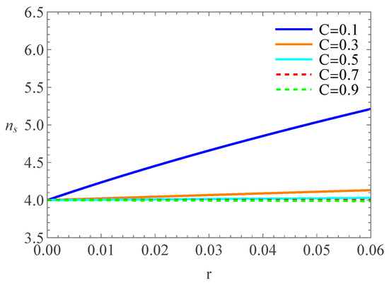
Solving Equation (16) yields the solution for $\lambda$; then, by substituting $\lambda$ into Equation (15), one can write $n_s$ as a function of r. The relation between $n_s$ and r is plotted in Figure 1, with C being the only free parameter. This figure shows that as C increases, the lines overlap and become indistinguishable for $C>0.7$. As can be seen in this figure, $n_s$ is larger than $4.0$, which is significantly higher than the Planck 2018 constraint $n_s=0.9668\pm 0.0037$ [8] and the ACT DR6 constraint $n_s=0.9743\pm 0.0034$ [9], indicating that this model is ruled out by observations. Consequently, similar to the case in the HDE model based on anti-de Sitter black hole entropy [18], within the framework of RHDE, holographic inflation is also not observationally viable. It should be noted, however, that holographic inflation is realized in other HDE models employing different IR cutoffs [108,111,112].

Figure 1. Relation between $n_s$ and r for holographic inflation within RHDE.

3. Slow-Roll Inflation

In the previous section, we have demonstrated that holographic inflation in the RHDE model is inconsistent with observations from Planck 2018 results and ACT DR6. In this section, we examine whether slow-roll inflation within RHDE is consistent with observational constraints.

3.1. Slow-Roll Dynamics

In the standard slow-roll inflation, under the slow-roll approximations ${\displaystyle \frac{1}{2}}{\dot{\varphi }}^2\ll V\left(\varphi \right)$ and $|\ddot{\varphi }|\ll |3H\dot{\varphi }|$, one can obtain the relation $H^2$∼$V\left(\varphi \right)$, which indicates $V\left(\varphi \right)$ is of the same order of magnitude as $H^2$. Then, in the framework of RHDE, under the slow-roll approximations, Equations (3) and (5) can be expressed as

$$\begin{array}{cc}& {\displaystyle H^2\approx \frac{{\kappa }^2}{3}V+\frac{C^2{H}^2}{1+\frac{8{\pi }^2\delta }{{\kappa }^2{H}^2}},}\end{array}$$

(17)

$$\begin{array}{cc}& 3H\dot{\varphi }+V_{,\varphi }\approx 0.\end{array}$$

(18)

From the above equation, and given that $\delta$ is much smaller than the inflationary scale $H^2$, we can conclude $\delta \ll H^2$ as a self-consistency condition. Under this condition, the dynamical equations for RHDE approximately reduce to those in the standard HDE. Therefore, the effect of $\delta$ is negligible, and the perturbation equations are the same as in the standard HDE. In the standard HDE, it is assumed that inflation is driven by the scalar field and that the HDE only affects the background dynamics without influencing the perturbations [94,115]. Under this assumption, the scalar spectral index $n_s$ and the tensor-to-scalar ratio r are expressed as [115]

$$\begin{array}{cc}& n_s=1-8ϵ+2\eta +2\sigma ,\end{array}$$

(19)

$$\begin{array}{cc}& r=16ϵ.\end{array}$$

(20)

with

$$\begin{array}{c}\hfill {\displaystyle ϵ=-\frac{\dot{H}}{H^2},\eta =-\frac{\ddot{\varphi }}{H\dot{\varphi }},\sigma =\frac{{\kappa }^2{\dot{\varphi }}^2}{H^2}.}\end{array}$$

(21)

Based on the above discussion, in order to study slow-roll inflation within the framework of RHDE, we adopt the same scalar spectral index (19) and the tensor-to-scalar ratio (20).

Then, differentiating Equation (17) yields

$$\dot{H}=-{\displaystyle \frac{{\kappa }^2}{4(1-C^2)}}\left[1+{\displaystyle \frac{48(1-2C^2){\pi }^2\delta +2{\kappa }^{4}V}{2\sqrt{576{\pi }^4{\delta }^2+48{\kappa }^4(1-2C^2){\pi }^2\delta V+{\kappa }^8{V}^2}}}\right]{\left({\displaystyle \frac{V_{,\varphi }}{3H}}\right)}^2.$$

(22)

Using Equations (17), (18) and (22), the slow-roll parameters $ϵ$, $\eta$ and $\sigma$ can be expressed as

$$\begin{array}{cc}& {\displaystyle ϵ=\frac{{\kappa }^2}{4(1-C^2)}\left[1+\frac{48(1-2C^2){\pi }^2\delta +2{\kappa }^{4}V}{2\sqrt{576{\pi }^4{\delta }^2+48{\kappa }^4(1-2C^2){\pi }^2\delta V+{\kappa }^8{V}^2}}\right]{\left(\frac{V_{,\varphi }}{3H^2}\right)}^2,}\end{array}$$

(23)

$$\begin{array}{cc}& {\displaystyle \eta =-ϵ+\frac{V_{,\varphi \varphi }}{3H^2},}\end{array}$$

(24)

$$\begin{array}{cc}& {\displaystyle \sigma ={\kappa }^2{\left(\frac{V_{,\varphi }}{3H^2}\right)}^2.}\end{array}$$

(25)

To compute the values of $n_s$ and r, we take the power-law potential $V\left(\varphi \right)$ to be of the form

$$V=V_0{\varphi }^n,$$

(26)

which is known as the chaotic potential, with both $V_0$ and n being positive parameters. Then, the slow-roll parameters $ϵ$, $\eta$ and $\sigma$ become

$$\begin{array}{cc}& {\displaystyle ϵ=\frac{{\kappa }^2}{4(1-C^2)}\left[1+\frac{48(1-2C^2){\pi }^2\left(\frac{\delta }{V_0}\right)+2{\kappa }^4{\varphi }^n}{2\xi }\right]{\left[\frac{2{\kappa }^2(1-C^2)n{\varphi }^{n-1}}{{\kappa }^4{\varphi }^n-24{\pi }^2\left(\frac{\delta }{V_0}\right)+\xi }\right]}^2,}\end{array}$$

(27)

$$\begin{array}{cc}& {\displaystyle \eta =-ϵ+\frac{2{\kappa }^2(1-C^2)n(n-1){\varphi }^{n-2}}{{\kappa }^4{\varphi }^n-24{\pi }^2\left(\frac{\delta }{V_0}\right)+\xi },}\end{array}$$

(28)

$$\begin{array}{cc}& {\displaystyle \sigma ={\kappa }^2{\left[\frac{2{\kappa }^2(1-C^2)n{\varphi }^{n-1}}{{\kappa }^4{\varphi }^n-24{\pi }^2\left(\frac{\delta }{V_0}\right)+\xi }\right]}^2,}\end{array}$$

(29)

with

$$\xi =\sqrt{576{\pi }^4{\left({\displaystyle \frac{\delta }{V_0}}\right)}^2+48{\kappa }^4(1-2C^2){\pi }^2\left({\displaystyle \frac{\delta }{V_0}}\right){\varphi }^n+{\kappa }^8{\varphi }^{2n}}$$

(30)

Then, substituting Equations (27), (28) and (29) into (19) and (20), the scalar spectral index $n_s$ and the tensor-to-scalar ratio r can be calculated. By considering $\delta \ll H^2$, we obtain $\delta \ll V$ and adopt ${10}^{-4}<{\displaystyle \frac{\delta }{V_0}}<{10}^{-2}$ for the following discussion, a range which ensures that the RHDE correction to the standard HDE is small but non-negligible, allowing us to study its observational implications for inflation. For HDE, without CMB data the parameter C is constrained to $C>1$, while the inclusion of CMB data forces $C<1$ [116]. Moreover, for ${\displaystyle \frac{\delta }{V_0}}\ll 1$, RHDE approximates HDE. Since this paper uses CMB data (ACT DR6) to analyze inflation, the constraints that include CMB data are more applicable. For these reasons, we adopt $C<1$ in the following discussion.

To examine the e-folds number N during inflation, we adopt the range $50\le N\le 70$, from which N can be expressed as

$$N=ln\left({\displaystyle \frac{a_e}{a_i}}\right)={\int }_{t_i}^{t_e}Hdt=-{\int }_{{\varphi }_i}^{{\varphi }_e}{\displaystyle \frac{3H^2}{V_{,\varphi }}}d\varphi .$$

(31)

where the subscript _e and _i denote the times when inflation ended and began, respectively. ${\varphi }_e$ is the scalar field at the end of inflation and can be solved from the relation ${ϵ}_e\simeq 1$. By inserting ${\varphi }_e$ into Equation (31), we obtain ${\varphi }_i$ as a function of N, but owing to the power exponent n, this function does not admit an analytical form and must be evaluated numerically. Then, substituting ${\varphi }_i$ into the calculated expressions for $n_s$ and r, we can express $n_s$ and r in terms of N. Different from the holographic inflation in the previous section, the expressions for $n_s$, and r in slow-roll inflation depend on the parameters $C^2$, ${\displaystyle \frac{\delta }{V_0}}$, n, and N, and cannot be expressed analytically. Accordingly, we perform numerical calculations for the cases $n={\displaystyle \frac{1}{2}}$ and $n={\displaystyle \frac{1}{3}}$ and display their relationships using figures.

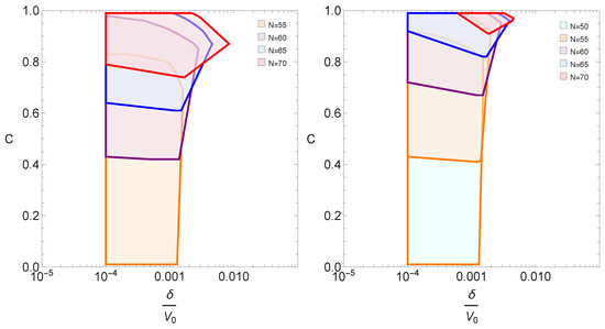
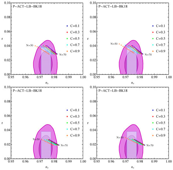
To determine the values of the parameters and match our results with the observations, we adopt the constraints $r<0.038$ [113] and $n_s=0.9743\pm 0.0034$ [9]. Then, for the cases $n={\displaystyle \frac{1}{2}}$ and $n={\displaystyle \frac{1}{3}}$, we plot the prediction regions in the $C-{\displaystyle \frac{\delta }{V_0}}$ plane with different e-fold numbers N, as shown in Figure 2; in the left panel, the case $n={\displaystyle \frac{1}{2}}$ is plotted with $N=55,60,65,70$ since $N=50$ in the parameter space does not satisfy the constraints $r<0.038$ and $n_s=0.9743\pm 0.0034$. These figures show that with the decrease in N, a larger C is required, and the allowed region in the $C-{\displaystyle \frac{\delta }{V_0}}$ plane becomes smaller; as n decreases, the allowed region for a given N shifts upward. Specifically, for $n={\displaystyle \frac{1}{2}}$ with $N=60$, $C>0.42$ is required; while for $n={\displaystyle \frac{1}{3}}$ with $N=60$, $C>0.67$ is needed. Within the adopted range ${10}^{-4}<{\displaystyle \frac{\delta }{V_0}}<{10}^{-2}$, the results prefer a smaller value of ${\displaystyle \frac{\delta }{V_0}}$.

Figure 2. Prediction regions in $C-{\displaystyle \frac{\delta }{V_0}}$ plane for slow-roll inflation within RHDE. The left panel is plotted for $n={\displaystyle \frac{1}{2}}$, while the right one is for $n={\displaystyle \frac{1}{3}}$.

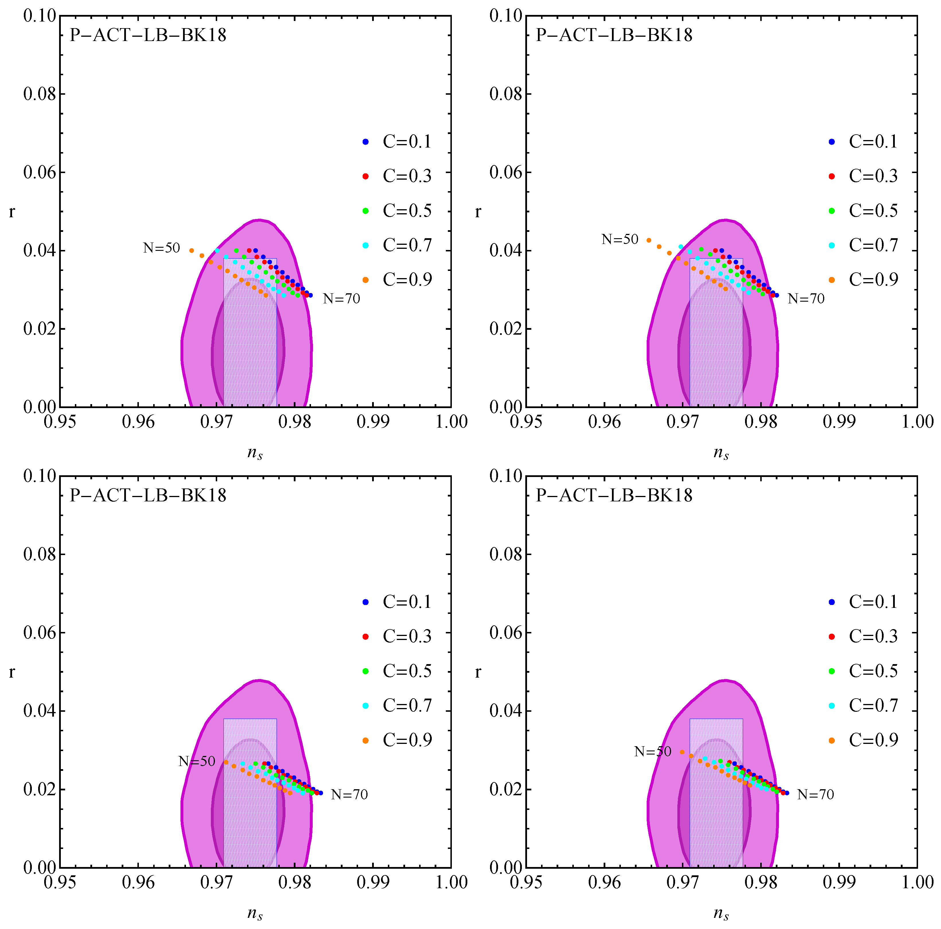
By fixing the parameters ${\displaystyle \frac{\delta }{V_0}}$ and n, we plot the predictions of the power-law potential (26) in the r-$n_s$ plane for four parameter sets in Figure 2, where we overlay our numerical results with the observational constraints from P-ACT-LB-BK18 [113], and the light blue rectangle denotes the constraints $r<0.038$ and $n_s=0.9743\pm 0.0034$. Compared to the first and second panels, the results favor a smaller ${\displaystyle \frac{\delta }{V_0}}$; the third and fourth panels also show this preference. Compared to the first and third panels, the results favor a smaller n; the second and fourth panels also show this preference. Compared to the cases $n={\displaystyle \frac{1}{2}}$ and $n={\displaystyle \frac{1}{3}}$, it can be seen from Figure 3 that an increase in n causes $n_s$ to shift to lower values and r to shift to higher values. As is shown in all panels, an increase in N leads to $n_s$ increasing and r decreasing and an increase in C leads to $n_s$ decreasing. In comparison with the observational constraints from P-ACT-LB-BK18, the results favor a larger C and a smaller n. It is evident that an increasing n or a decreasing C could cause a mismatch with the observations. Nevertheless, for both cases $n={\displaystyle \frac{1}{2}}$ and $n={\displaystyle \frac{1}{3}}$, a suitable choice of N and C remains favored by the observational data. Notably, the power-law potential (26) in standard slow-roll inflation is ruled out by the Planck 2018 results [12] and is disfavored by ACT DR6 [113]. However, slow-roll inflation is realized within RHDE and is supported by ACT DR6.

Figure 3. Predictions of the power-law potential (26) in the r-$n_s$ plane for four parameter sets: (1) $n={\displaystyle \frac{1}{2}},{\displaystyle \frac{\delta }{V_0}}={10}^{-4}$, (2) $n={\displaystyle \frac{1}{2}},{\displaystyle \frac{\delta }{V_0}}={10}^{-3}$, (3) $n={\displaystyle \frac{1}{3}},{\displaystyle \frac{\delta }{V_0}}={10}^{-4}$, (4) $n={\displaystyle \frac{1}{3}},{\displaystyle \frac{\delta }{V_0}}={10}^{-3}$.

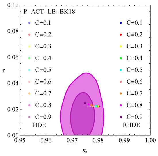
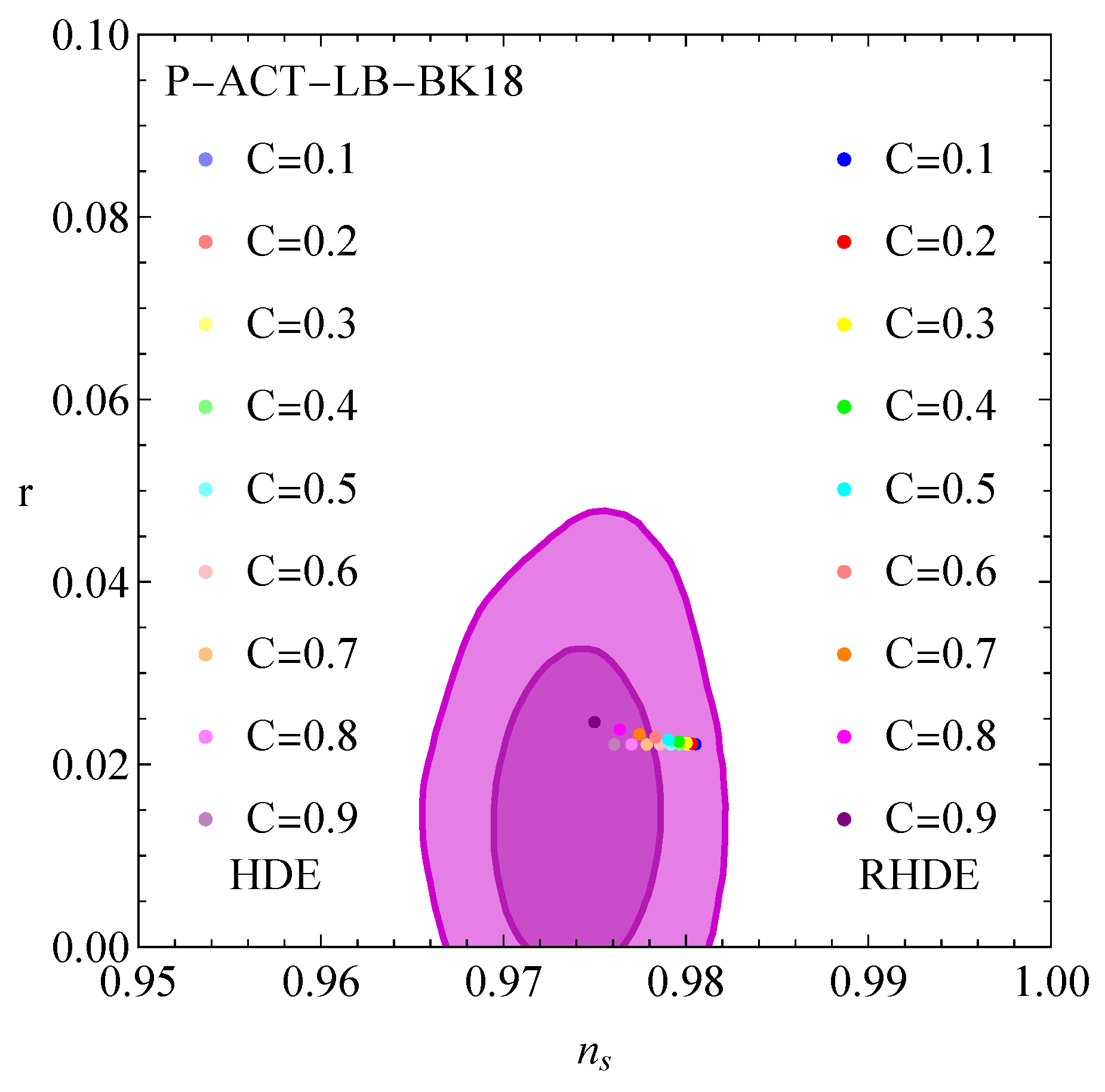
In Figure 4, we compare the results for HDE and RHDE in the r-$n_s$ plane, for which we take $N=60$; light-colored points denote the results obtained from HDE, while dark-colored points correspond to RHDE results with ${\displaystyle \frac{\delta }{V_0}}={10}^{-3}$. This figure shows that with the increase in C, the difference between RHDE and HDE becomes obvious, and RHDE has a larger r and a smaller $n_s$.

Figure 4. Predictions of the power-law potential (26) for slow-roll inflation with $N=60$ within HDE and RHDE in the r-$n_s$ plane. Light-colored points denote the results obtained from HDE, while dark-colored points correspond to RHDE results with ${\displaystyle \frac{\delta }{V_0}}={10}^{-3}$.

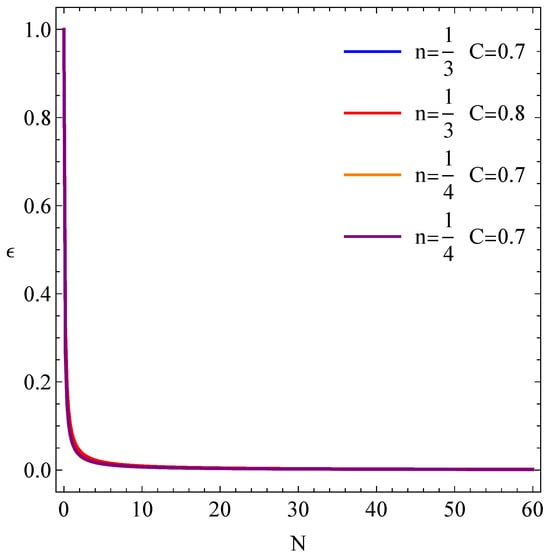
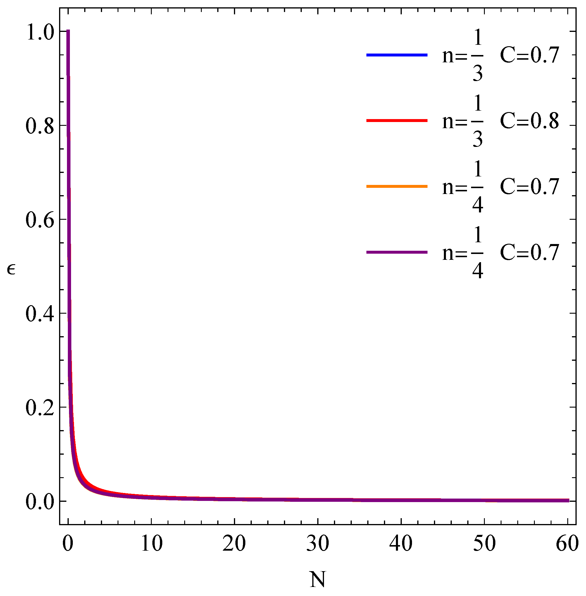
To examine whether inflation ends naturally within the RHDE framework, we plot the evolutionary curves for the slow-roll parameter $ϵ$ as a function of N, as shown in Figure 5. Here, N denotes the remaining e-folds, $N=60$ corresponds to the onset of the slow-roll regime, while $N=0$ denotes the end of inflation. With the decrease in N, $ϵ$ increases and becomes equal to 1 at $N=0$, indicating that the slow-roll approximation gradually breaks down and inflation terminates naturally. This behavior is consistent with the standard slow-roll inflation scenario and confirms that the RHDE framework does not prevent a graceful exit from inflation.

Figure 5. Slow-roll parameter $ϵ$ versus N with ${\displaystyle \frac{\delta }{V_0}}={10}^{-3}$. Here, N represents the remaining e-folds.

After inflation ended, the universe evolved into the hot expansion era, successively undergoing the radiation-dominated, matter-dominated, and dark energy-dominated epochs. To describe the evolution of the universe after inflation, dynamical analysis is proposed and widely used as a method for studying this process [117,118,119,120,121,122,123,124,125,126,127,128]. For RHDE, statefinder diagnostic [98] and phase space analysis [105] have been successfully used to analyze the evolution of the universe after inflation.

3.2. Inflationary Attractor

It is well known that inflationary models with canonical scalar fields exhibit cosmological attractor behavior [129]. This behavior plays a crucial role in viable scenarios by ensuring theoretical consistency across different initial conditions. The attractor behavior of the solution can be studied using both analytical and numerical methods. In this subsection, we analyze the attractor behavior within RHDE and examine whether our analytical solution acts as an attractor.

Using Equations (17) and (18), we obtain the analytical solutions for the slow-roll inflation within RHDE as follows

$$\dot{\varphi }=-{\displaystyle \frac{n{V}_0{\varphi }^{n-1}}{3}}{\left[{\displaystyle \frac{6{\kappa }^2(1-C^2)}{{\kappa }^4{V}_0{\varphi }^n-24{\pi }^2\delta +\sqrt{576{\pi }^4{\delta }^2+48{\kappa }^4(1-2C^2){\pi }^2\delta V_0{\varphi }^n+{\kappa }^8{V}_0^2{\varphi }^{2n}}}}\right]}^{{\displaystyle \frac{1}{2}}}.$$

(32)

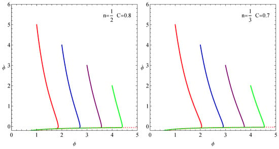
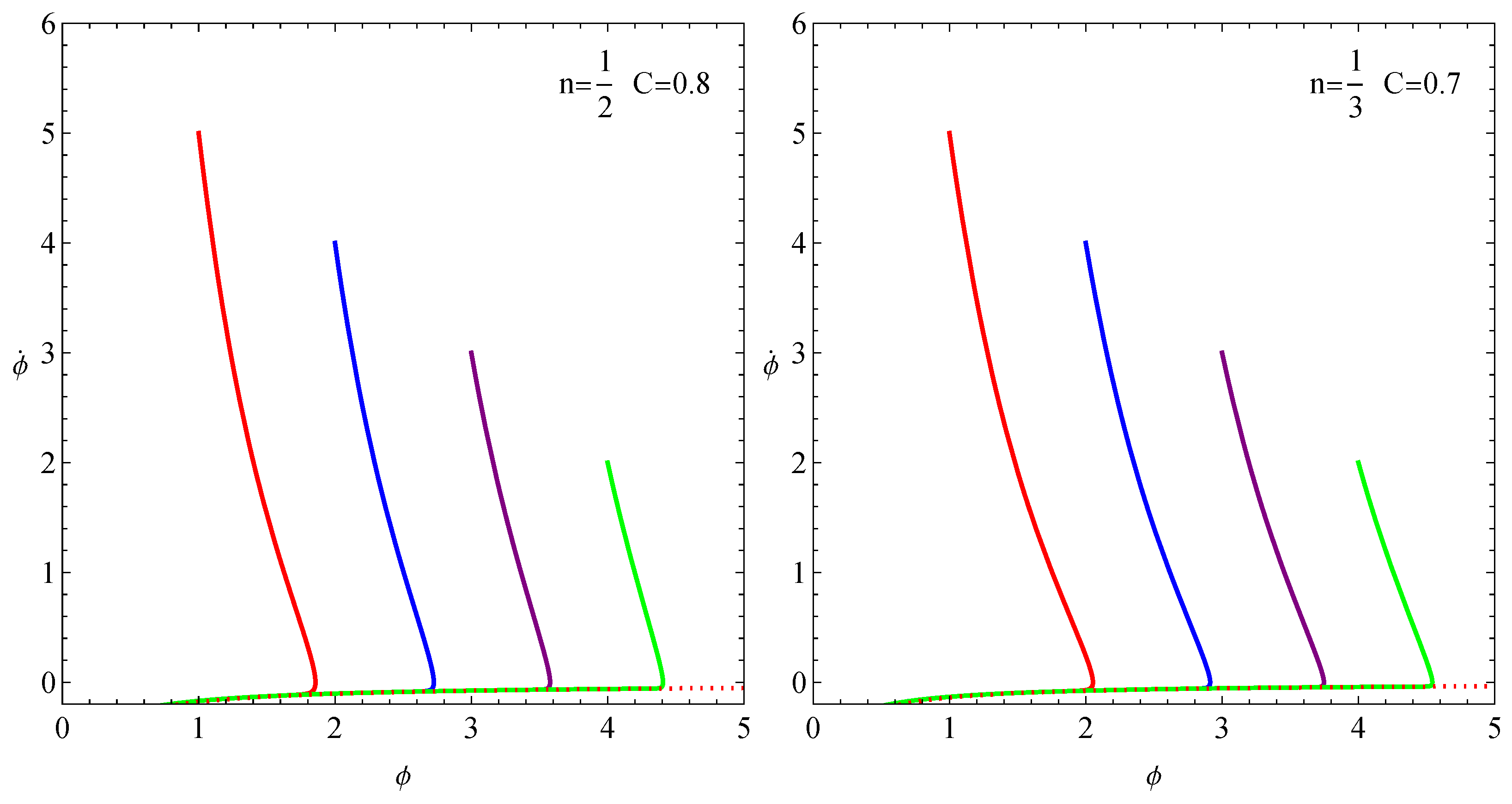
With different initial conditions, we numerically solve Equations (3) and (5) and present the resulting phase space diagram in Figure 6, where the dotted lines represent the corresponding analytical solutions. These figures demonstrate that, regardless of the initial conditions, the kinetic energy rapidly decays to a negligible value, thereby driving the inflation field into a potential-dominated slow-roll state. The evolutionary trajectories exhibit strong convergence and ultimately approach the analytical solution indicated by the red-dotted lines. Consequently, within the framework of RHDE, the analytical solution serves as an attractor.

Figure 6. Phase space diagram for the power-law potential (26) within RHDE. The red dotted lines represent the analytical solution of the attractor, while the solid lines denote the evolutionary curves of the numerical solutions with different initial conditions.

3.3. Primordial Power Spectrum

In the first subsection, we analyze the slow-roll inflation within RHDE and adopt the CMB pivot scale $k_{CMB}=0.05Mp{c}^{-1}$. In this subsection, we present the full shape of the curvature power spectrum on all scales. To achieve this goal, under the slow-roll condition, we numerically solve the background Equations (3) and (5) together with the Mukhanov–Sasaki equation

$$v_k^{\prime \prime }+\left(k^2-{\displaystyle \frac{z^{″}}{z}}\right)v_k=0,$$

(33)

where a prime ′ denotes the derivative with respect to conformal time $\eta$, and $z={\displaystyle \frac{a\dot{\varphi }}{H}}$. Then, the power spectrum of primordial curvature perturbations ${\mathcal{P}}_{\mathcal{R}}\left(k\right)$ is given by

$${\mathcal{P}}_{\mathcal{R}}\left(k\right)={\displaystyle \frac{k^3}{2{\pi }^2}}{\left|{\displaystyle \frac{v_k}{z}}\right|}^2.$$

(34)

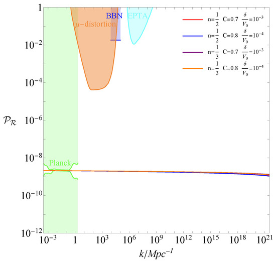
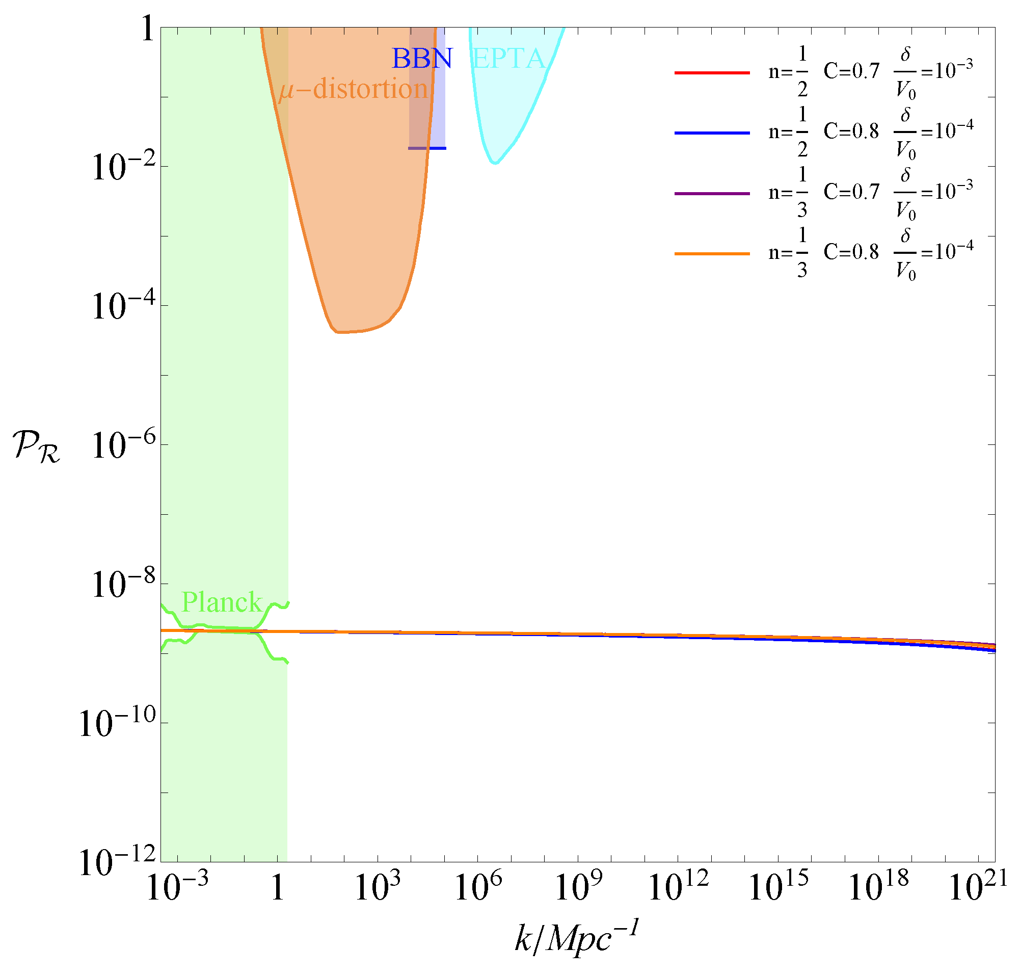
Adopting the initial conditions listed in Table 1, which are chosen according to the results in the first subsection, we numerically solve these equations to obtain the primordial power spectrum. Our numerical results are listed in Table 1 and shown in Figure 7, where they are superimposed on the observational data from CMB [8], $\mu$-distortion of CMB [130], big-bang nucleosynthesis (BBN [131]), and the European Pulsar Timing Array (EPTA [132]). It can be seen that our numerical results for the primordial curvature power spectra fall well within the bounds set by current observations. This confirms that the RHDE model, with the considered parameter space, is fully compatible with current multi-probe observational data. Therefore, the inflationary predictions derived from the RHDE framework are observationally viable and warrant further investigation in light of future high-precision measurements.

Table 1. Model parameters and the numerical results for primordial power spectrum within RHDE.

Model	n	C	$\mathit{\delta }$	${\mathit{V}}_0$	$\frac{\mathit{\delta }}{{\mathit{V}}_0}$	${\mathit{N}}_{*}$	${\mathit{n}}_{\mathit{s}}$	r	${\mathcal{P}}_{\mathcal{R}}\left({\mathit{k}}_{*}\right)$
A	${\displaystyle \frac{1}{2}}$	$0.7$	$1.28\times {10}^{-10}$	$1.28\times {10}^{-7}$	${10}^{-3}$	$59.53$	$0.9748$	$0.0342$	$2.108\times {10}^{-9}$
B	${\displaystyle \frac{1}{2}}$	$0.8$	$9.60\times {10}^{-12}$	$9.60\times {10}^{-8}$	${10}^{-4}$	$59.35$	$0.9735$	$0.0338$	$2.103\times {10}^{-9}$
C	${\displaystyle \frac{1}{3}}$	$0.7$	$4.18\times {10}^{-10}$	$4.18\times {10}^{-7}$	${10}^{-3}$	$59.77$	$0.9773$	$0.0234$	$2.108\times {10}^{-9}$
D	${\displaystyle \frac{1}{3}}$	$0.8$	$3.00\times {10}^{-11}$	$3.00\times {10}^{-7}$	${10}^{-4}$	$57.27$	$0.9762$	$0.0231$	$2.105\times {10}^{-9}$

Figure 7. Results for the primordial curvature perturbation power spectrum ${\mathcal{P}}_{\mathcal{R}}\left(k\right)$ within RHDE.

4. Conclusions

Based on the Rényi entropy, Rényi holographic dark energy has been proposed to explain the current accelerated phase of the universe. In this paper, we analyze holographic inflation and slow-roll inflation within the framework of RHDE. For the holographic inflation, we find it is ruled out by ACT DR6, since for $r<0.06$, the predicted $n_s$ exceeds the observationally allowed range. For slow-roll inflation with the power-law potential $V_0{\varphi }^n$, we find that the observational constraints from P-ACT-LB-BK18 favor a larger C and a smaller n, while for both cases $n={\displaystyle \frac{1}{2}}$ and $n={\displaystyle \frac{1}{3}}$, a suitable choice of N and C is favored by the observational data.

Then, we analyze the inflationary attractor within RHDE. By solving the background dynamical equation and plotting the evolutionary curves in $\dot{\varphi }-\varphi$ plane, we find that the evolutionary trajectories exhibit strong convergence and ultimately approach the analytical solution. This indicates that the analytical solution acts as an attractor. Additionally, we adopt the value of model parameters constrained by the observational data and numerically solve the background equations together with the Mukhanov–Sasaki equation, we plot the curves for the primordial curvature power spectrum and find our numerical results fall well within the bounds set by the observational data from CMB, $\mu$-distortion of CMB, big-bang nucleosynthesis, and the European Pulsar Timing Array. All results demonstrate that within the RHDE framework, slow-roll inflation is observationally viable, while holographic inflation is not supported by current observational data.

References

- Guth, A. The Inflationary Universe: A Possible Solution to the Horizon and Flatness Problems. Phys. Rev. D 1981, 23, 347. [Google Scholar] [CrossRef] [Scilit]
- Linde, A. A New Inflationary Universe Scenario: A Possible Solution of the Horizon, Flatness, Homogeneity, Isotropy and Primordial Monopole Problems. Phys. Lett. B 1982, 108, 389. [Google Scholar] [CrossRef] [Scilit]
- Mukhanov, V.; Chibisov, G. Quantum Fluctuations and a Nonsingular Universe. JETP Lett. 1981, 33, 532. [Google Scholar]
- Lewis, A.; Challinor, A.; Lasenby, A. Efficient computation of CMB anisotropies in closed FRW models. Astrophys. J. 2000, 538, 473. [Google Scholar] [CrossRef] [Scilit]
- Bernardeau, F.; Colombi, S.; Gaztanaga, E.; Scoccimarro, R. Large scale structure of the universe and cosmological perturbation theory. Phys. Rep. 2002, 367, 1. [Google Scholar] [CrossRef] [Scilit]
- Smoot, G.; Bennett, C.; Kogut, A.; Wright, E.; Aymon, J.; Boggess, N.; Cheng, E.; Amici, G.D.; Gulkis, S.; Hauser, M.; et al. Structure in the COBE differential microwave radiometer first year maps. Astrophys. J. 1992, 396, L1. [Google Scholar] [CrossRef] [Scilit]
- Hinshaw, G.; Larson, D.; Komatsu, E.; Spergel, D.; Bennett, C.; Dunkley, J.; Nolta, M.; Halpern, M.; Hill, R.; Odegard, N.; et al. Nine-Year Wilkinson Microwave Anisotropy Probe (WMAP) Observations: Cosmological parameter results. Astrophys. J. Suppl. Ser. 2013, 208, 19. [Google Scholar] [CrossRef] [Scilit]
- Planck Collaboration. Planck 2018 results. VI. Cosmological parameters. Astron. Astrophys. 2020, 641, A6. [Google Scholar] [CrossRef] [Scilit]
- Louis, T.; Posta, A.; Atkins, Z.; Jense, H.; Abril-Cabezas, I.; Addison, G.; Ade, P.; Aiola, S.; Alford, T.; Alonso, D.; et al. The Atacama Cosmology Telescope: DR6 power spectra, likelihoods and ΛCDM parameters. J. Cosmol. Astropart. Phys. 2025, 11, 062. [Google Scholar] [CrossRef] [Scilit]
- Noh, H.; Hwang, J. Inflationary spectra in generalized gravity: Unified forms. Phys. Lett. B 2001, 515, 231. [Google Scholar] [CrossRef] [Scilit]
- Weinberg, S. Cosmology; Oxford University Press: Oxford, UK, 2008. [Google Scholar]
- Planck Collaboration. Planck 2018 results. X. Constraints on inflation. Astron. Astrophys. 2020, 641, A10. [Google Scholar] [CrossRef] [Scilit]
- Maggiore, M. Gravitational Waves; Oxford University Press: Oxford, UK, 2018. [Google Scholar]
- Ellis, J.; Garcia, M.; Olive, K.; Verner, S. Constraints on attractor models of inflation and reheating from Planck, BICEP/Keck, ACT DR6, and SPT-3G data. Phys. Rev. D 2026, 113, 063571. [Google Scholar] [CrossRef] [Scilit]
- Yuennan, J.; Eadkhong, T.; Atamurotov, F.; Channuie, P. Constraining non-minimally coupled squared-quartic hilltop inflation in light of ACT observations. Phys. Dark Universe 2026, 52, 102282. [Google Scholar] [CrossRef] [Scilit]
- Ketov, S.; Pozdeeva, E.; Vernov, S. Inflation in F(R) gravity models revisited after ACT. J. Cosmol. Astropart. Phys. 2025, 12, 040. [Google Scholar] [CrossRef] [Scilit]
- Keskin, A.; Canpolat, L.; Kurt, K. Slow-rolling and quintessence inflation with the D-brane KKLT potential in Barrow entropy. Eur. Phys. J. C 2025, 85, 634. [Google Scholar] [CrossRef] [Scilit]
- Huang, Q.; Huang, H.; Xu, B.; Zhang, K. Holographic inflation and holographic dark energy from entropy of the anti-de Sitter black hole. Eur. Phys. J. C 2025, 85, 395. [Google Scholar] [CrossRef] [Scilit]
- Ding, G.; Jiang, S.; Zhao, W. Modular invariant slow roll inflation. J. Cosmol. Astropart. Phys. 2024, 10, 016. [Google Scholar] [CrossRef] [Scilit]
- Ragavendra, H.; Sarkar, A.; Sethi, S. Constraining ultra slow roll inflation using cosmological datasets. J. Cosmol. Astropart. Phys. 2024, 7, 088. [Google Scholar] [CrossRef] [Scilit]
- Pozdeeva, E.; Skugoreva, M.; Toporensky, A.; Vernov, S. New slow-roll approximations for inflation in Einstein-Gauss-Bonnet gravity. J. Cosmol. Astropart. Phys. 2024, 9, 050. [Google Scholar] [CrossRef] [Scilit]
- Zhang, F.; Yu, H.; Lin, W. Inflation and reheating predictions in f(T)-gravity. Phys. Dark Universe 2024, 44, 101482. [Google Scholar] [CrossRef] [Scilit]
- Marco, A.; Orazi, E.; Pradisi, G. Introduction to the Number of e-Folds in Slow-Roll Inflation. Universe 2024, 10, 284. [Google Scholar] [CrossRef] [Scilit]
- Lambiase, G.; Luciano, G.; Sheykhi, A. Slow-roll inflation and growth of perturbations in Kaniadakis modification of Friedmann cosmology. Eur. Phys. J. C 2023, 83, 936. [Google Scholar] [CrossRef] [Scilit]
- Afshar, B.; Moradpour, H.; Shabani, H. Slow-roll inflation and reheating in Rastall theory. Phys. Dark Universe 2023, 42, 101357. [Google Scholar] [CrossRef] [Scilit]
- Bhat, A.; Mandal, S.; Sahoo, P. Slow-roll inflation in f(T,) modified gravity. Chin. Phys. C 2023, 47, 125104. [Google Scholar] [CrossRef] [Scilit]
- Dioguardi, C.; Racioppi, A.; Tomberg, E. Slow-roll inflation in Palatini F(R) gravity. J. High Energy Phys. 2022, 6, 106. [Google Scholar] [CrossRef] [Scilit]
- Karciauskas, M.; Diaz, J. Slow-roll inflation in the Jordan frame. Phys. Rev. D 2022, 106, 083526. [Google Scholar] [CrossRef] [Scilit]
- Chen, C.; Reyimuaji, Y.; Zhang, X. Slow-roll inflation in f(R,T) gravity with a RT mixing term. Phys. Dark Universe 2022, 38, 101130. [Google Scholar] [CrossRef] [Scilit]
- Capozziello, S.; Shokri, M. Slow-roll inflation in f(Q) non-metric gravity. Phys. Dark Universe 2022, 37, 101113. [Google Scholar] [CrossRef] [Scilit]
- Forconi, M.; Giare, W.; Valentino, E.; Melchiorri, A. Cosmological constraints on slow roll inflation: An update. Phys. Rev. D 2021, 104, 103528. [Google Scholar] [CrossRef] [Scilit]
- Cai, R.; Chen, C.; Fu, C. Primordial black holes and stochastic gravitational wave background from inflation with a noncanonical spectator field. Phys. Rev. D 2021, 104, 083537. [Google Scholar] [CrossRef] [Scilit]
- Gamonal, M. Slow-roll inflation in f(R,T) gravity and a modified Starobinsky-like inflationary model. Phys. Dark Universe 2021, 31, 100768. [Google Scholar] [CrossRef] [Scilit]
- Fu, C.; Wu, P.; Yu, H. Primordial black holes and oscillating gravitational waves in slow-roll and slow-climb inflation with an intermediate noninflationary phase. Phys. Rev. D 2020, 102, 043527. [Google Scholar] [CrossRef] [Scilit]
- Akin, K.; Arapoglu, A.; Yukselci, A. Formalizing slow-roll inflation in scalar-tensor theories of gravitation. Phys. Dark Universe 2020, 30, 100691. [Google Scholar] [CrossRef] [Scilit]
- Fu, C.; Wu, P.; Yu, H. Primordial Black Holes from Inflation with Nonminimal Derivative Coupling. Phys. Rev. D 2019, 100, 063532. [Google Scholar] [CrossRef] [Scilit]
- Granda, L.; Jimenez, D. Slow-Roll Inflation in Scalar-Tensor Models. J. Cosmol. Astropart. Phys. 2019, 9, 007. [Google Scholar] [CrossRef] [Scilit]
- Gonzalez-Espinoza, M.; Otalora, G.; Videla, N.; Saavedra, J. Slow-roll inflation in generalized scalar-torsion gravity. J. Cosmol. Astropart. Phys. 2019, 8, 029. [Google Scholar] [CrossRef] [Scilit]
- Granda, L.; Jimenez, D. Slow-Roll Inflation with Exponential Potential in Scalar-Tensor Models. Eur. Phys. J. C 2019, 79, 772. [Google Scholar] [CrossRef] [Scilit]
- Yi, Z.; Gong, Y.; Sabir, M. Inflation with Gauss-Bonnet coupling. Phys. Rev. D 2018, 98, 083521. [Google Scholar] [CrossRef] [Scilit]
- Casadio, R.; Giugno, A.; Giusti, A. Corpuscular slow-roll inflation. Phys. Rev. D 2018, 97, 024041. [Google Scholar] [CrossRef] [Scilit]
- Odintsov, S.; Oikonomou, V. Reconstruction of Slow-roll F(R) Gravity Inflation from the Observational Indices. Ann. Phys. 2018, 388, 267. [Google Scholar] [CrossRef] [Scilit]
- Tahmasebzadeh, B.; Rezazadeh, K.; Karami, K. Brans-Dicke inflation in light of the Planck 2015 data. J. Cosmol. Astropart. Phys. 2016, 7, 006. [Google Scholar] [CrossRef] [Scilit]
- Yang, N.; Gao, Q.; Gong, Y. Inflation with non-minimally derivative coupling. Int. J. Mode. Phys. A 2015, 30, 1545004. [Google Scholar] [CrossRef] [Scilit]
- Koh, S. Observational constraints on slow-roll inflation coupled to a Gauss-Bonnet term. Phys. Rev. D 2014, 90, 063527. [Google Scholar] [CrossRef] [Scilit]
- Gao, Q.; Gong, Y.; Li, T.; Ye, T. Simple single field inflation models and the running of spectral index. Sci. China Phys. Mech. Astron. 2014, 57, 1442. [Google Scholar] [CrossRef] [Scilit]
- Antusch, S.; Nolde, D. BICEP2 implications for single-field slow-roll inflation revisited. J. Cosmol. Astropart. Phys. 2014, 5, 035. [Google Scholar] [CrossRef] [Scilit]
- Guo, Z.; Schwarz, D. Slow-roll inflation with a Gauss-Bonnet correction. Phys. Rev. D 2010, 81, 123520. [Google Scholar] [CrossRef] [Scilit]
- Satoh, M. Slow-roll Inflation with the Gauss-Bonnet and Chern-Simons Corrections. J. Cosmol. Astropart. Phys. 2010, 11, 024. [Google Scholar] [CrossRef] [Scilit]
- Kaneda, S.; Ketov, S.; Watanabe, N. Slow-roll inflation in (R+R4) gravity. Class. Quantum Grav. 2010, 27, 145016. [Google Scholar] [CrossRef] [Scilit]
- Brax, P.; Bruck, C.; Hall, L.; Weller, J. Slow-Roll Inflation in the Presence of a Dark Energy Coupling. Phys. Rev. D 2009, 79, 103508. [Google Scholar] [CrossRef] [Scilit]
- Tzirakis, K.; Kinney, W. Non-canonical generalizations of slow-roll inflation models. J. Cosmol. Astropart. Phys. 2009, 1, 028. [Google Scholar] [CrossRef] [Scilit]
- Barenboim, G.; Kinney, W. Slow roll in simple non-canonical inflation. J. Cosmol. Astropart. Phys. 2007, 3, 014. [Google Scholar] [CrossRef] [Scilit]
- Peiris, H.; Easther, R. Slow Roll Reconstruction: Constraints on Inflation from the 3 Year WMAP Dataset. J. Cosmol. Astropart. Phys. 2006, 10, 017. [Google Scholar] [CrossRef] [Scilit]
- Gong, Y. Constraints on inflation in Einstein-Brans-Dicke frame. Phys. Rev. D 1999, 59, 083507. [Google Scholar] [CrossRef] [Scilit]
- Yi, Z.; Wang, X.; Gao, Q.; Gong, Y. Approximate reconstruction of inflationary potential with ACT observations. Phys. Lett. B 2025, 871, 140002. [Google Scholar] [CrossRef] [Scilit]
- Choudhury, S. Reconstructing inflationary potential from NANOGrav 15-year data: A robust study using Non-Bunch Davies initial condition. J. High Energy Astrophys. 2024, 44, 220. [Google Scholar] [CrossRef] [Scilit]
- Choi, K.; Gong, J.; Kang, S.; Raveendran, R. Potential reconstruction from general power spectrum in single-field inflation. J. Cosmol. Astropart. Phys. 2022, 1, 012. [Google Scholar] [CrossRef] [Scilit]
- Fei, Q.; Yi, Z.; Yang, Y. The Reconstruction of Non-Minimal Derivative Coupling Inflationary Potentials. Universe 2020, 6, 213. [Google Scholar] [CrossRef] [Scilit]
- Barrow, J.; Paliathanasis, A. Reconstructions of the dark-energy equation of state and the inflationary potential. Gen. Relativ. Gravit. 2018, 50, 82. [Google Scholar] [CrossRef] [Scilit]
- Gao, Q.; Gong, Y. Reconstruction of extended inflationary potentials for attractors. Eur. Phys. J. Plus 2018, 133, 491. [Google Scholar] [CrossRef] [Scilit]
- Koh, S.; Lee, B.; Tumurtushaa, G. Reconstruction of the Scalar Field Potential in Inflationary Models with a Gauss-Bonnet term. Phys. Rev. D 2017, 95, 123509. [Google Scholar] [CrossRef] [Scilit]
- Fei, Q.; Gong, Y.; Lin, J.; Yi, Z. The reconstruction of tachyon inflationary potentials. J. Cosmol. Astropart. Phys. 2017, 8, 018. [Google Scholar] [CrossRef] [Scilit]
- Lin, J.; Gao, Q.; Gong, Y. The reconstruction of inflationary potentials. Mon. Not. Roy. Astron. Soc. 2016, 459, 4029. [Google Scholar] [CrossRef] [Scilit]
- Cline, J.; Hoi, L. Inflationary potential reconstruction for a wmap running power spectrum. J. Cosmol. Astropart. Phys. 2006, 6, 007. [Google Scholar] [CrossRef] [Scilit]
- Easther, R.; Kinney, W. Monte Carlo reconstruction of the inflationary potential. Phys. Rev. D 2003, 67, 043511. [Google Scholar] [CrossRef] [Scilit]
- Adams, F.; Freese, K. The Scalar field potential in inflationary models: Reconstruction and further constraints. Phys. Rev. D 1995, 51, 6722. [Google Scholar] [CrossRef] [Scilit]
- Liddle, A.; Turner, M. Second order reconstruction of the inflationary potential. Phys. Rev. D 1994, 50, 758. [Google Scholar] [CrossRef] [Scilit]
- Motohashi, H.; Starobinsky, A.; Yokoyama, J. Inflation with a constant rate of roll. J. Cosmol. Astropart. Phys. 2015, 9, 018. [Google Scholar] [CrossRef] [Scilit]
- Gao, Q. Reconstruction of constant slow-roll inflation. Sci. China Phys. Mech. Astron. 2017, 60, 090411. [Google Scholar] [CrossRef] [Scilit]
- Gao, Q.; Gong, Y.; Fei, Q. Constant-roll tachyon inflation and observational constraints. J. Cosmol. Astropart. Phys. 2018, 5, 005. [Google Scholar] [CrossRef] [Scilit]
- Yi, Z.; Gong, Y. On the constant-roll inflation. J. Cosmol. Astropart. Phys. 2018, 3, 052. [Google Scholar] [CrossRef] [Scilit]
- Gao, Q. The observational constraint on constant-roll inflation. Sci. China Phys. Mech. Astron. 2018, 61, 70411. [Google Scholar] [CrossRef] [Scilit]
- Motohashi, H.; Starobinsky, A. Constant-roll inflation in scalar-tensor gravity. J. Cosmol. Astropart. Phys. 2019, 11, 025. [Google Scholar] [CrossRef] [Scilit]
- Gao, Q.; Gong, Y.; Yi, Z. On the constant-roll inflation with large and small ηH. Universe 2019, 5, 215. [Google Scholar] [CrossRef] [Scilit]
- Ravanpak, A.; Fadakar, G. Constant-roll inflation in brane induced gravity cosmology. Eur. Phys. J. C 2022, 82, 924. [Google Scholar] [CrossRef] [Scilit]
- Mohammadi, A. Constant-roll inflation driven by holographic dark energy. Phys. Dark Universe 2022, 36, 101055. [Google Scholar] [CrossRef] [Scilit]
- Shokri, M.; Sadeghi, J.; Gashti, S. Quintessential constant-roll inflation. Phys. Dark Universe 2022, 35, 100923. [Google Scholar] [CrossRef] [Scilit]
- Panda, S.; Rana, A.; Thakur, R. Constant-roll inflation in modified f(R,ϕ) gravity model using Palatini formalism. Eur. Phys. J. C 2023, 83, 297. [Google Scholar] [CrossRef] [Scilit]
- Liu, J.; Gong, Y.; Yi, Z. Constant-roll inflation with non-minimally derivative coupling. Commun. Theor. Phys. 2024, 76, 095401. [Google Scholar] [CrossRef] [Scilit]
- Huang, Q.; Chen, L.; Huang, H.; Xu, B.; Zhang, K. Constant-roll inflation and primordial black holes within Barrow entropic framework. Phys. Dark Universe 2025, 50, 102072. [Google Scholar] [CrossRef] [Scilit]
- Thavanesan, A.; Werth, D.; Handley, W. Analytical approximations for curved primordial power spectra. Phys. Rev. D 2021, 103, 023519. [Google Scholar] [CrossRef] [Scilit]
- Shumaylov, Z.; Handley, W. Primordial power spectra from k-inflation with curvature. Phys. Rev. D 2022, 105, 123532. [Google Scholar] [CrossRef] [Scilit]
- Huang, Q.; Zhang, K.; Fang, Z.; Tu, F. Analytical approximations for primordial power spectra in a spatially closed emergent universe. Phys. Dark Universe 2022, 38, 101124. [Google Scholar] [CrossRef] [Scilit]
- Huang, Q.; Huang, H.; Xu, B. CMB power spectrum for emergent scenario and slow expansion in scalar-tensor theory of gravity. Phys. Dark Universe 2023, 41, 101262. [Google Scholar] [CrossRef] [Scilit]
- Liu, Z.; Zhang, J.; Piao, Y. A Galileon Design of Slow Expansion. Phys. Rev. D 2011, 84, 063508. [Google Scholar] [CrossRef] [Scilit]
- Liu, Z.; Piao, Y. A Galileon Design of Slow Expansion: Emergent universe. Phys. Lett. B 2013, 718, 734. [Google Scholar] [CrossRef] [Scilit]
- Cai, Y.; Piao, Y. The slow expansion with nonminimal derivative coupling and its conformal dual. J. High Energy Phys. 2016, 3, 134. [Google Scholar] [CrossRef] [Scilit]
- Cohen, A.; Kaplan, D.; Nelson, A. Effective field theory, black holes, and the cosmological constant. Phys. Rev. Lett. 1999, 82, 4971. [Google Scholar] [CrossRef] [Scilit]
- Susskind, L. The World as a hologram. J. Math. Phys. 1995, 36, 6377. [Google Scholar] [CrossRef] [Scilit]
- Bousso, R. The Holographic principle. Rev. Mod. Phys. 2002, 74, 825. [Google Scholar] [CrossRef] [Scilit]
- Hsu, S. Entropy bounds and dark energy. Phys. Lett. B 2004, 594, 13. [Google Scholar] [CrossRef] [Scilit]
- Li, M. A Model of holographic dark energy. Phys. Lett. B 2004, 603, 1. [Google Scholar] [CrossRef] [Scilit]
- Wang, S.; Wang, Y.; Li, M. Holographic Dark Energy. Phys. Rep. 2017, 696, 1. [Google Scholar] [CrossRef] [Scilit]
- Moradpour, H.; Moosavi, S.; Lobo, I.; Graca, J.M.; Jawad, A.; Salako, I. Thermodynamic approach to holographic dark energy and the Rényi entropy. Eur. Phys. J. C 2018, 78, 829. [Google Scholar] [CrossRef] [Scilit]
- Ghaffari, S.; Ziaie, A.; Bezerra, V.; Moradpour, H. Inflation in the Rényi cosmology. Mod. Phys. Lett. A 2019, 35, 1950341. [Google Scholar] [CrossRef] [Scilit]
- Iqbal, A.; Jawad, A. Tsallis, Renyi and Sharma-Mittal holographic dark energy models in DGP brane-world. Phys. Dark Universe 2019, 26, 100349. [Google Scholar] [CrossRef] [Scilit]
- Sharma, U.; Dubey, V. Rényi holographic dark energy in the Brans-Dicke cosmology. Mod. Phys. Lett. A 2020, 35, 2050281. [Google Scholar] [CrossRef] [Scilit]
- Sharma, U.; Dubey, V. Statefinder diagnostic for the Rényi holographic dark energy. New Astron. 2020, 80, 101419. [Google Scholar] [CrossRef] [Scilit]
- Saha, A.; Ghose, S.; Chanda, A.; Paul, B. Rényi Holographic Dark Energy in Higher Dimension Cosmology. Ann. Phys. 2021, 426, 168403. [Google Scholar] [CrossRef] [Scilit]
- Shekh, S.; Moraes, P.; Sahoo, P. Physical Acceptability of the Renyi, Tsallis and Sharma-Mittal Holographic Dark Energy Models in the f(T,B) Gravity under Hubble’s Cutoff. Universe 2021, 7, 67. [Google Scholar] [CrossRef] [Scilit]
- Sardar, A.; Debnath, U. Cosmological consequences of Rényi, Sharma-Mittal holographic and new agegraphic dark energy models in generalized Rastall gravity. Mod. Phys. Lett. A 2021, 36, 2150180. [Google Scholar] [CrossRef] [Scilit]
- Saha, A.; Chanda, A.; Dey, S.; Ghose, S.; Paul, B. Interacting and non-interacting Rényi holographic dark energy models in DGP braneworld. Mod. Phys. Lett. A 2023, 38, 2350024. [Google Scholar] [CrossRef] [Scilit]
- Manoharan, M.; Shaji, N.; Mathew, T. Holographic dark energy from the laws of thermodynamics with Rényi entropy. Eur. Phys. J. C 2023, 83, 19. [Google Scholar] [CrossRef] [Scilit]
- Das, S.; Mahata, N. Phase space analysis of Rényi Holographic dark energy model. Gen. Rel. Grav. 2025, 57, 120. [Google Scholar] [CrossRef] [Scilit]
- Abdelrashied, M.; Aly, A.; Selim, M. Studying Thermal and Dynamical Stability of Interacting Rényi and Tsallis Holographic Dark Energy Models in LTB Inhomogeneous Universe. Res. Astron. Astrophys. 2025, 25, 025012. [Google Scholar] [CrossRef] [Scilit]
- Prasanthi, U.D.; Aditya, Y. Observational constraints on Renyi holographic dark energy in Kantowski–Sachs universe. Phys. Dark Universe 2021, 31, 100782. [Google Scholar] [CrossRef] [Scilit]
- Nojiri, S.; Odintsov, S.; Saridakis, E. Holographic inflation. Phys. Lett. B 2019, 797, 134829. [Google Scholar] [CrossRef] [Scilit]
- Granda, L.; Oliveros, A. Infrared cut-off proposal for the Holographic density. Phys. Lett. B 2008, 669, 275. [Google Scholar] [CrossRef] [Scilit]
- Granda, L.; Oliveros, A. New infrared cut-off for the holographic scalar fields models of dark energy. Phys. Lett. B 2009, 671, 199. [Google Scholar] [CrossRef] [Scilit]
- Oliveros, A.; Acero, M. Inflation driven by a holographic energy density. Europhys. Lett. 2019, 128, 59001. [Google Scholar] [CrossRef] [Scilit]
- Mohammadi, A.; Golanbari, T.; Bamba, K.; Lobo, I. Tsallis holographic dark energy for inflation. Phys. Rev. D 2021, 103, 083505. [Google Scholar] [CrossRef] [Scilit]
- Calabrese, E.; Hill, J.; Jense, H.; Posta, A.; Abril-Cabezas, I.; Addison, G.; Ade, P.; Aiola, S.; Alford, T.; Alonso, D.; et al. The Atacama Cosmology Telescope: DR6 Constraints on Extended Cosmological Models. J. Cosmol. Astropart. Phys. 2025, 11, 063. [Google Scholar] [CrossRef] [Scilit]
- Martin, J.; Ringeval, C.; Vennin, V. Encyclopædia Inflationaris. Phys. Dark Universe 2014, 5–6, 75. [Google Scholar] [CrossRef] [Scilit]
- Chen, B.; Li, M.; Wang, Y. Inflation with Holographic Dark Energy. Nucl. Phys. B 2007, 774, 256. [Google Scholar] [CrossRef] [Scilit]
- Li, T.; Li, Y.; Du, G.; Wu, P.; Feng, L.; Zhang, J.; Zhang, X. Revisiting holographic dark energy after DESI 2024. Eur. Phys. J. C 2025, 85, 608. [Google Scholar] [CrossRef] [Scilit]
- Bahamonde, S.; Bohmer, C.; Carloni, S.; Copeland, E.; Fang, W.; Tamanini, N. Dynamical systems applied to cosmology: Dark energy and modified gravity. Phys. Rep. 2018, 775–777, 1. [Google Scholar] [CrossRef] [Scilit]
- Huang, Q.; Huang, H.; Chen, J.; Zhang, L.; Tu, F. Stability analysis of a Tsallis holographic dark energy model. Class. Quantum Grav. 2019, 36, 175001. [Google Scholar] [CrossRef] [Scilit]
- Huang, Q.; Huang, H.; Xu, B.; Tu, F.; Chen, J. Dynamical analysis and statefinder of Barrow holographic dark energy. Eur. Phys. J. C 2021, 81, 686. [Google Scholar] [CrossRef] [Scilit]
- Wu, P.; Yu, H. The dynamical behavior of f(T) theory. Phys. Lett. B 2010, 692, 176. [Google Scholar] [CrossRef] [Scilit]
- Wu, P.; Zhang, S. Cosmological evolution of interacting phantom (quintessence) model in Loop Quantum Gravity. J. Cosmol. Astropart. Phys. 2008, 6, 7. [Google Scholar] [CrossRef] [Scilit]
- Wu, P.; Yu, H. Class. Interacting generalized Chaplygin gas. Quant. Grav. 2007, 24, 4661. [Google Scholar] [CrossRef] [Scilit]
- Dutta, J.; Khyllep, W.; Tamanini, N. Cosmological dynamics of scalar fields with kinetic corrections: Beyond the exponential potential. Phys. Rev. D 2016, 93, 063004. [Google Scholar] [CrossRef] [Scilit]
- Dutta, J.; Khyllep, W.; Tamanini, N. Scalar-Fluid interacting dark energy: Cosmological dynamics beyond the exponential potential. Phys. Rev. D 2017, 95, 023515. [Google Scholar] [CrossRef] [Scilit]
- Dutta, J.; Khyllep, W.; Zonunmawia, H. Cosmological dynamics of the general non-canonical scalar field models. Eur. Phys. J. C 2019, 79, 359. [Google Scholar] [CrossRef] [Scilit]
- Huang, Y.; Gao, Q.; Gong, Y. The Phase-space analysis of scalar fields with non-minimally derivative coupling. Eur. Phys. J. C 2015, 75, 143. [Google Scholar] [CrossRef] [Scilit]
- Chen, X.; Gong, Y.; Saridakis, E. Phase-space analysis of interacting phantom cosmology. J. Cosmol. Astropart. Phys. 2009, 4, 001. [Google Scholar] [CrossRef] [Scilit]
- Chatterjee, A.; Gong, Y. Understanding curvature–matter interaction in viable f(R) dark energy models: A dynamical analysis approach. Ann. Phys. 2025, 478, 170036. [Google Scholar] [CrossRef] [Scilit]
- Remmen, G.; Carroll, S. Attractor Solutions in Scalar-Field Cosmology. Phys. Rev. D 2013, 88, 083518. [Google Scholar] [CrossRef] [Scilit]
- Fixsen, D.; Cheng, E.; Gales, J.; Mather, J.; Shafer, R.; Wright, E. The Cosmic Microwave Background spectrum from the full COBE FIRAS data set. Astrophys. J. 1996, 473, 576. [Google Scholar] [CrossRef] [Scilit]
- Inomata, K.; Kawasaki, M.; Tada, Y. Revisiting constraints on small scale perturbations from big-bang nucleosynthesis. Phys. Rev. D 2016, 94, 043527. [Google Scholar] [CrossRef] [Scilit]
- Inomata, K.; Nakama, T. Gravitational waves induced by scalar perturbations as probes of the small-scale primordial spectrum. Phys. Rev. D 2019, 99, 043511. [Google Scholar] [CrossRef] [Scilit]
Disclaimer/Publisher’s Note: The statements, opinions and data contained in all publications are solely those of the individual author(s) and contributor(s) and not of MDPI and/or the editor(s). MDPI and/or the editor(s) disclaim responsibility for any injury to people or property resulting from any ideas, methods, instructions or products referred to in the content. |
© 2026 by the authors. Licensee MDPI, Basel, Switzerland. This article is an open access article distributed under the terms and conditions of the Creative Commons Attribution (CC BY) license.