Chaotic Motion of Strings in a Quantum-Corrected AdS Reissner–Nordström Black Hole

Abstract

It has been reported that quantum correction modifies the topological charges of Anti-de-Sitter Reissner–Nordström (AdS-RN) black holes in Kiselev spacetime, yielding new perspectives on topological classification. This leads us to focus on how quantum corrections and other parameters collectively influence the long-term dynamic evolution of strings. First, we analytically examine whether the strings’ motion violates the Maldacena–Shenker–Stanford (MSS) bound. Then, we employ numerical integration to study the influence of various parameters on string chaotic dynamics. Our results demonstrate that the quantum-correction parameter a, the normalization factor c, and black-hole charge Q significantly influence chaotic behavior and the violation of the MSS bound. In particular, as a increases, the system undergoes an order–chaos–order transition, whereas an increase in c or a decrease in Q drives the system from order to chaos.

1. Introduction

Chaos is a hallmark of deterministic nonlinear dynamical systems, characterized by long-term unpredictability due to extreme sensitivity to initial conditions. Investigating chaotic dynamics in strong gravitational fields, particularly in the highly curved spacetime of black holes, not only elucidates the nonlinear interplay between gravity and matter but also bridges general relativity, quantum gravity, and dynamical systems theory [1,2,3,4,5,6,7,8,9,10,11,12,13,14,15,16,17,18,19,20,21,22,23,24,25]. The chaotic nature of the motion of matter near a black-hole horizon directly impacts the theoretical interpretation of astrophysical phenomena such as accretion, gravitational lensing, and gravitational-wave emission. In a fixed curved spacetime, the geodesic motion of structureless test particles is often integrable; for instance, in typical Kerr–Newman black hole backgrounds, sufficient conserved quantities ensure regularity [26]. By contrast, relativistic strings—one-dimensional extended objects—possess infinitely many vibrational degrees of freedom, and their dynamics are governed by a two-dimensional worldsheet, offering a far richer potential for nonlinearity and chaos. This complexity stems not only from the string’s self-interaction but also from its deep connections to quantum-gravity frameworks such as the AdS/CFT correspondence. Hence, the chaotic behavior of strings reflects the combined nonlinearities of the background spacetime geometry and the extended structure of the string itself. Even in flat spacetime, string-vibration equations exhibit nonlinear traits; in extreme gravitational environments like black holes, their motion is expected to display highly complex chaotic dynamics [14,27,28,29,30,31]. Consequently, strings serve as a unique probe for exploring the microscopic structure of spacetime, testing the limits of classical determinism, and seeking signatures of quantum-gravity effects.

Quantifying chaos is a central theoretical challenge. The Maldacena–Shenker–Stanford (MSS) bound sets a universal upper limit on the Lyapunov exponent for finite-temperature quantum systems [6], forging a deep link between quantum chaos and black-hole thermodynamics. This bound provides a key benchmark for understanding chaotic properties in strongly coupled many-body systems within the holographic-duality framework. As a result, studying how the chaotic behavior of gravitational or quantum systems approaches or violates this bound has emerged as an important research direction [24,32,33]. Yet most existing work concentrates on classical black-hole backgrounds; the influence of quantum corrections—typically encoded in deformation parameters—on chaotic dynamics and possible MSS-bound violations remains largely unexplored. Quantum corrections offer a crucial route to addressing the singularity problem of classical general relativity and probing spacetime microstructure. For example, the classical Schwarzschild solution possesses a curvature singularity at $r=0$. By including spherical quantum fluctuations of the metric and matter fields, Kazakov and Solodukhin built an effective two-dimensional quantum-gravity model whose quantum-corrected Schwarzschild solution replaces the singularity with a region of finite curvature with a minimal radius of Planck-scale order, thus resolving the classical singularity and yielding a finite scalar curvature [34]. Such corrections show that quantum effects can eliminate classical singularities while substantially modifying black-hole thermodynamics, phase structure, and geometry. These modifications give rise to novel phenomena in black-hole criticality and thermodynamic responses (e.g., the Joule–Thomson effect) [35,36,37,38,39]. Studying chaotic dynamics in quantum-corrected black-hole spacetimes—especially with respect to how quantum-correction parameters affect the onset, evolution, and possible violation of bounds such as the MSS bound—is therefore a natural and necessary theoretical extension. This approach not only yields a more realistic picture of potential quantum-gravity imprints in strong-field regimes but also opens a new avenue for systematically exploring the interrelations among quantum geometry, matter fields, and chaotic dynamics in a semi-classical gravitational setting.

Kiselev spacetime furnishes an important framework for studying black holes surrounded by anisotropic matter fields. Its metric describes a central gravitational source embedded in a fluid with a prescribed equation of state. Within this framework, chaotic dynamics and thermodynamic properties around black holes have been examined from various angles. For example, Gao et al. [7] used Lyapunov exponents to analyze test-particle motion in a Kiselev black-hole background, showing that angular momentum and black-hole charge strongly influence the violation of the chaos bound. Simultaneously, Sadeghi et al. [40] built a quantum-corrected Anti-de Sitter Reissner–Nordström (AdS-RN) black hole in this setting and studied its thermodynamic topology via the generalized off-shell Helmholtz free-energy method, finding that the quantum-correction term plays a key role in the topological classification of black holes. These studies illustrate that the AdS-RN black hole in Kiselev spacetime provides a comprehensive model incorporating anisotropic matter, electric charge, and a cosmological constant. It thus offers a fertile ground for investigating non-asymptotically flat spacetimes with complex matter–energy distributions. Adding quantum corrections further enables a more realistic simulation of semi-classical gravitational effects within the model, creating a platform that blends physical richness with theoretical self-consistency for studying the chaotic dynamical evolution of strings (as opposed to point particles) in such complex geometries.

Because string motion is inherently nonlinear, numerical methods are essential for characterizing its chaotic dynamics. Simulating chaotic string dynamics in Kiselev spacetime poses two main challenges: (1) Traditional numerical schemes tend to accumulate energy errors during long-term integration, potentially generating spurious chaos [41]. (2) The equations of motion are highly nonlinear and admit no analytical solution. Hence, choosing an integrator that yields reliable results over long integration times is critical. Fortunately, a symplectic algorithm can preserve the geometric structure of Hamiltonian systems; it is the tool of choice for conservative systems [42,43,44,45,46,47,48,49,50]. These algorithms conserve energy and momentum exactly at the numerical level, thereby avoiding the spurious chaos caused by energy drift in traditional methods like the Runge–Kutta method during long-term simulations [51]. It has been reported that implicit symplectic algorithms (e.g., the high-order methods developed by Feng based on the implicit-midpoint rule [52]) are usually more computationally costly and less efficient in implementation than explicit symplectic algorithms of the same order. Their advantage is that they can be applied directly to general systems without Hamiltonian splitting, and all phase-space variables are solved fully implicitly, making them particularly suited for non-separable Hamiltonians. Conversely, explicit symplectic algorithms, such as those introduced by Ruth et al., require that the Hamiltonian be split into kinetic and potential parts [53]. Extensive work has demonstrated that explicit symplectic algorithms are generally not directly applicable to non-separable systems. For separable Hamiltonian systems, explicit symplectic algorithms are more favorable, as they strike a balance between accuracy and computational efficiency. Explicit symplectic algorithms usually decompose the Hamiltonian into exactly integrable pieces ($H_A$) and perturbative pieces ($H_B$) and then build iterative schemes via symmetric operators (e.g., ${\Phi }_h=e^{h{L}_{H_A}/2}\circ e^{h{L}_{H_B}/2}\circ e^{h{L}_{H_A}/2}$, where L denotes the Lie derivative and h denotes step size). The construction of such integrators for dynamics in black-hole backgrounds has progressed considerably. In particular, the multi-part splitting method has been successfully used in various curved spacetimes. For example, Wang et al. [45] split the Hamiltonian for charged-particle motion near a magnetized Schwarzschild black hole into four terms, designing a four-part explicit symplectic integrator. For the Reissner–Nordström case, the Hamiltonian splits into five parts, which are likewise amenable to use with explicit symplectic methods [46]. For a magnetized Anti-de Sitter Reissner–Nordström black hole, the Hamiltonian requires a six-term split [47]. Moreover, Wu et al. [48] built an explicit symplectic integrator for a Kerr black hole using the time-transformation technique developed by [49]. These developments have greatly advanced explicit symplectic integration in curved, strong-field spacetimes and spurred subsequent applications to dynamical evolution in more complex systems.

The motion of particles around charged black holes—including scenarios involving electromagnetic interactions between charged particles and background fields—has been extensively discussed in the literature. For instance, while particle motion around a Schwarzschild black hole is typically periodic, the inclusion of charge or magnetic fields, as in magnetized or charged Schwarzschild black holes, can induce chaotic behavior [54]. In Kerr–Newman spacetime, trajectories are generally quasi-periodic, whereas multi-black-hole configurations are known to readily lead to chaos [1,26,55]. Chaotic motion of charged particles has also been observed in the Melvin cosmological model [56]. Johannsen and Psaltis examined how the radii of innermost stable circular orbits and circular photon orbits vary with increasing spin and displacement parameters in rapidly rotating black holes [57]. Studies using Hořava–Lifshitz gravity have shown that an external magnetic field influences the radial motion of charged test particles and can give rise to chaotic dynamics [58]. Similar analyses have explored chaotic behavior around Schwarzschild-like black holes with deformation parameters under the influence of external magnetic fields [59]. Toshmatov et al. further investigated the motion of charged particles around Schwarzschild-like or Kerr-like black holes immersed in uniform external magnetic fields [60]. Hu and Huang [50] reported chaotic behavior in a magnetized brane-world spacetime, while Zhou et al. [61] examined irregular motion of charged particles around a magnetized Schwarzschild black hole. Cao et al. [62], in turn, explored electromagnetic configurations and chaotic signatures of charged particles near hairy black holes in Horndeski gravity. Moreover, Lu and Wu [63] assessed the role of two quantum-correction parameters in shaping the chaotic dynamics of particles near a modified Schwarzschild black hole within the re-normalization group approach. Recently, Xu et al. investigated the chaotic behavior of charged particles in Kerr–MOG black holes [64] and Gibbons–Maeda–Garfinkle–Horowitz–Strominger black holes [65]. Beyond the role of electromagnetic fields in driving chaos among charged particles, various astrophysically relevant scenarios have also attracted significant attention. For example, Ruffini and Wilson [66] discussed relativistic magnetohydrodynamic effects in plasma accretion onto black holes, while Stuchlík et al. [67] investigated the combined influence of cosmic repulsion and magnetic fields on accretion disks orbiting Kerr black holes.

The chaotic dynamics of strings parallel those of charged particles moving in a black hole’s magnetic field. In our previous work, we investigated the chaotic dynamics of strings in three distinct black hole backgrounds: a Gauss–Bonnet black hole in $Ad{S}_5$ space [12], a charged black brane with hyperscaling violation [13], and a regular black hole [14]. Our results showed that string motion exhibits significantly more pronounced chaotic behavior than particle motion, with ordered orbits being extremely rare—indeed, nearly all trajectories are chaotic. Building on these findings, this study shifts focus from a comparative analysis of particle and string dynamics to two primary objectives. First, we examine whether the string motion can surpass the MSS limit, a question typically approached through analytical methods centered on radial motion. Second, we explore the full spatial dynamical evolution of the string.

The paper is organized as follows. In Section 2, we provide the black-hole model and use analytical methods to discuss whether the motion of strings will exceed the MSS limit. In Section 3, we use a symplectic algorithm as a numerical integration tool to study the influence of various parameters on the chaotic dynamics of strings. Finally, Section 4 summarizes the results and conclusions.

2. The Black Hole and MSS Boundary Problem

2.1. Quantum-Corrected AdS Reissner–Nordstrom Black Holes in Kiselev Spacetime

Consistent with the description in [39,40], the metric for a quantum-corrected AdS-RN black hole embedded in Kiselev spacetime is expressed as follows:

$$d{s}^2=f\left(r\right)d{t}^2-{\displaystyle \frac{d{r}^2}{f\left(r\right)}}-r^2\left(d{\theta }^2+{sin}^2\theta d{\varphi }^2\right),$$

(1)

with

$$f\left(r\right)=-{\displaystyle \frac{2M}{r}}+{\displaystyle \frac{\sqrt{r^2-a^2}}{r}}+{\displaystyle \frac{r^2}{{\ell }^2}}-{\displaystyle \frac{c}{r^{3\omega +1}}}+{\displaystyle \frac{Q^2}{r^2}}.$$

(2)

Here, M denotes the black hole’s mass, Q is the charge, and ℓ is the AdS length scale (fixed at $\ell =15$). The parameter c represents a normalization factor, while a quantifies quantum corrections to the black hole’s mass. Theoretically, a may assume any value within the range [34,68] but must satisfy $a<r$ to ensure metric reality, consistent with its interpretation as a small quantum correction. Notably, setting $a=0$ recovers the standard AdS-RN black hole surrounded by a cosmological fluid.

The equation-of-state parameter $\omega$, characterizing the anisotropic fluid surrounding the black hole, determines the ambient matter’s nature: $\omega =0$ (ideal gas), $\omega ={\displaystyle \frac{1}{3}}$ (ultra-relativistic particles), $-1<\omega <-{\displaystyle \frac{1}{3}}$ (dark energy), $\omega =-1$ (the cosmological constant, in the isotropic case), and $\omega <-1$ (phantom dark energy). In this work, we focus on $\omega =-{\displaystyle \frac{1}{3}}$. This parameter spans key physical phases of the background fluid. Its associated exponential terms create couplings between the Kiselev fluid and quantum corrections that exhibit distinct characteristics, enabling us to explore how quantum corrections influence strings’ chaotic motion and modify the MSS bound [40,69,70].

For Equation (2), neglecting quantum corrections ($a=0$) and the Kiselev background yields the RN solution in AdS₄ spacetime:

$$f\left(r\right)=1-{\displaystyle \frac{2M}{r}}+{\displaystyle \frac{Q^2}{r^2}}+{\displaystyle \frac{r^2}{{\ell }^2}}.$$

(3)

Further disregarding the AdS background ($\ell \to \infty$), Equation (3) yields the asymptotically flat RN metric:

$$f\left(r\right)=1-{\displaystyle \frac{2M}{r}}+{\displaystyle \frac{Q^2}{r^2}}.$$

(4)

Now, we consider the motion of a string around the quantum-corrected AdS-RN black hole. Based on the Polyakov action [14],

$$\mathcal{L}=-{\displaystyle \frac{1}{2\pi {\alpha }^{\prime }}}\sqrt{-g}{g}^{\mu \nu }{G}_{ab}{\partial }_{\mu }{X}^a{\partial }_{\nu }{X}^b.$$

(5)

Here, the coupling constant ${\alpha }^{\prime }$ is connected to string length $l_s$ through the relation $l_s^2={\alpha }^{\prime }$; in this work, we set ${\alpha }^{\prime }={\displaystyle \frac{1}{\pi }}$. The symbol $X^a$ stands for the target-space coordinates, with $G_{ab}$ being the associated metric. Worldsheet coordinates are taken as ${\sigma }^{\mu }=(\tau ,\sigma )$, and the induced metric on the worldsheet is denoted by $g_{\mu \nu }$. We find it advantageous to impose the conformal gauge—i.e., $g_{\mu \nu }={\eta }_{\mu \nu }$. The following ansatz is then employed:

$$t=t\left(\tau \right),r=r\left(\tau \right),\theta =\theta \left(\tau \right),\varphi =\alpha \sigma .$$

(6)

The winding number $\alpha$ encodes the difference between string and point-particle behavior. Under the conditions chosen, the Hamiltonian takes the explicit form:

$$H={\displaystyle \frac{\pi {\alpha }^{\prime }}{2}}\left[f\left(r\right)p_r^2+{\displaystyle \frac{p_{\theta }^2}{r^2}}-{\displaystyle \frac{p_t^2}{f\left(r\right)}}\right]+{\displaystyle \frac{1}{2\pi {\alpha }^{\prime }}}{r}^2{\alpha }^2{sin}^2\theta .$$

(7)

It is worth noting that the Hamiltonian for a string closely resembles that of a relativistic particle in an electromagnetic field [45,46,47,48]. In this analogy, the string effectively plays the role of the electromagnetic potential in particle models. Naturally, the black hole solution $f\left(r\right)$ considered here also incorporates the effects of additional physical factors. As discussed in [44], the absence of a fourth integral—analogous to the Carter constant—can lead to chaotic behavior in particle motion. This conclusion also holds for the motion of strings.

2.2. Lyapunov Exponent

Lyapunov exponents are fundamental tools for characterizing chaotic behavior and have been extensively investigated in the literature [5,6,71,72,73,74,75,76], primarily through eigenvalue computations of the Jacobian matrix.

The analytical procedure commences with the string’s equations of motion:

$${\displaystyle \frac{d{X}_i\left(t\right)}{dt}}=F_i\left(X^j\right).$$

(8)

Linearization yields

$${\displaystyle \frac{d\delta X_i\left(t\right)}{dt}}=K_{ij}\left(t\right)\delta X_j\left(t\right),$$

(9)

where $K_{ij}\left(t\right)$ denotes the Jacobian matrix, defined as

$$K_{ij}\left(t\right)={\displaystyle \frac{\partial F_i}{\partial X_j}}{|}_{X_i\left(t\right)}.$$

(10)

Solutions to Equation (9) satisfy

$$\delta X_i\left(t\right)=L_{ij}\left(t\right)\delta X_j\left(0\right),$$

(11)

with $L_{ij}\left(t\right)$ being the evolution matrix, obeying $\dot{L_{ij}\left(t\right)}=K_{im}{L}_{mj}\left(t\right)$ and $L_{ij}\left(0\right)={\delta }_{ij}$. The Lyapunov exponent $\lambda$, quantifying the exponential divergence rate of adjacent trajectories, is then extracted from the eigenvalues of $L_{ij}\left(t\right)$ [5]:

$$\lambda =\underset{t\to \infty }{lim}{\displaystyle \frac{1}{t}}ln\left({\displaystyle \frac{\parallel L_{jj}\left(t\right)\parallel }{\parallel L_{jj}\left(0\right)\parallel }}\right).$$

(12)

Building upon [15], we analyze chaos in the radial momentum phase space $(r,p_r)$. The functional relations are defined as follows:

$$F_1={\displaystyle \frac{dr}{dt}}={\displaystyle \frac{\dot{r}}{\dot{t}}}=-{\displaystyle \frac{f^2{p}_r}{p_t}},$$

(13)

$$F_2={\displaystyle \frac{d{p}_r}{dt}}={\displaystyle \frac{{\dot{p}}_r}{\dot{t}}}={\displaystyle \frac{f^{\prime }{p}_t}{2f}}+{\displaystyle \frac{f{f}^{\prime }{p}_r^2}{2p_t}}-{\displaystyle \frac{p_{\theta }^{2}f}{r^3{p}_t}}+{\displaystyle \frac{{\alpha }^{2}r{sin}^2\theta f}{p_t}},$$

(14)

with $p_t=E$ (energy). Here, the dot denotes differentiation with respect to proper time $\tau$, while the prime denotes differentiation with respect to the radial coordinate r. The Jacobian matrix elements in this subspace are

$$\begin{array}{cc}\hfill K_{11}& ={\displaystyle \frac{\partial F_1}{\partial r}}=-{\displaystyle \frac{{\left(f^2\right)}^{\prime }{p}_r}{E}},\hfill \\ \hfill K_{12}& ={\displaystyle \frac{\partial F_1}{\partial p_r}}=-{\displaystyle \frac{f^2}{E}},\hfill \\ \hfill K_{21}& ={\displaystyle \frac{\partial F_2}{\partial r}}={\displaystyle \frac{f^{″}E}{2f}}-{\displaystyle \frac{f^{\prime 2}E}{2f^2}}+{\displaystyle \frac{\left(f^{\prime }f\right)p_r^2}{2E}}-{\displaystyle \frac{p_{\theta }^2{f}^{\prime }}{r^{3}E}}+{\displaystyle \frac{3p_{\theta }^{2}f}{r^{4}E}}+{\displaystyle \frac{{\left({\alpha }^{2}rf\right)}^{\prime }{sin}^2\theta }{E}},\hfill \\ \hfill K_{22}& ={\displaystyle \frac{\partial F_2}{\partial p_r}}={\displaystyle \frac{p_{r}f{f}^{\prime }}{E}}.\hfill \end{array}$$

(15)

Finally, by imposing the radial equilibrium constraints $p_r={\dot{p}}_r=0$, we derive the simplified explicit expression for the Lyapunov exponent:

$${\lambda }^2=-{\displaystyle \frac{f^{″}f}{2}}+{\displaystyle \frac{f^{\prime 2}}{2}}+{\displaystyle \frac{p_{\theta }^2{f}^{\prime }{f}^2}{r^3{E}^2}}-{\displaystyle \frac{3p_{\theta }^2{f}^3}{r^4{E}^2}}-{\displaystyle \frac{f^2{\left({\alpha }^{2}rf\right)}^{\prime }sin\theta }{E^2}}.$$

(16)

2.3. Violation of the MSS Bound

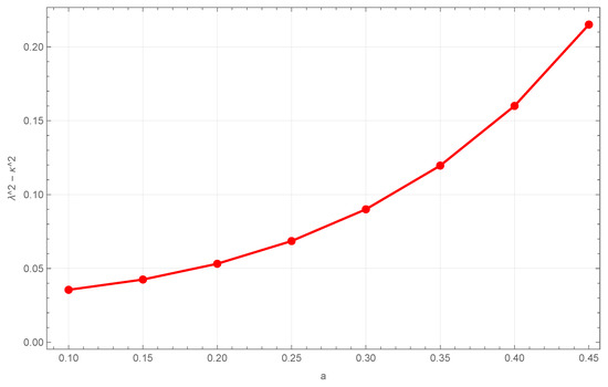
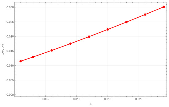
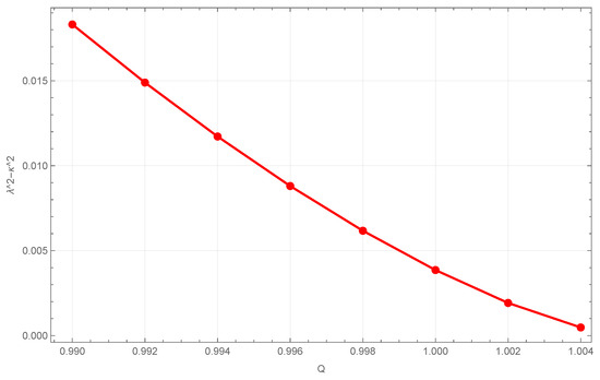
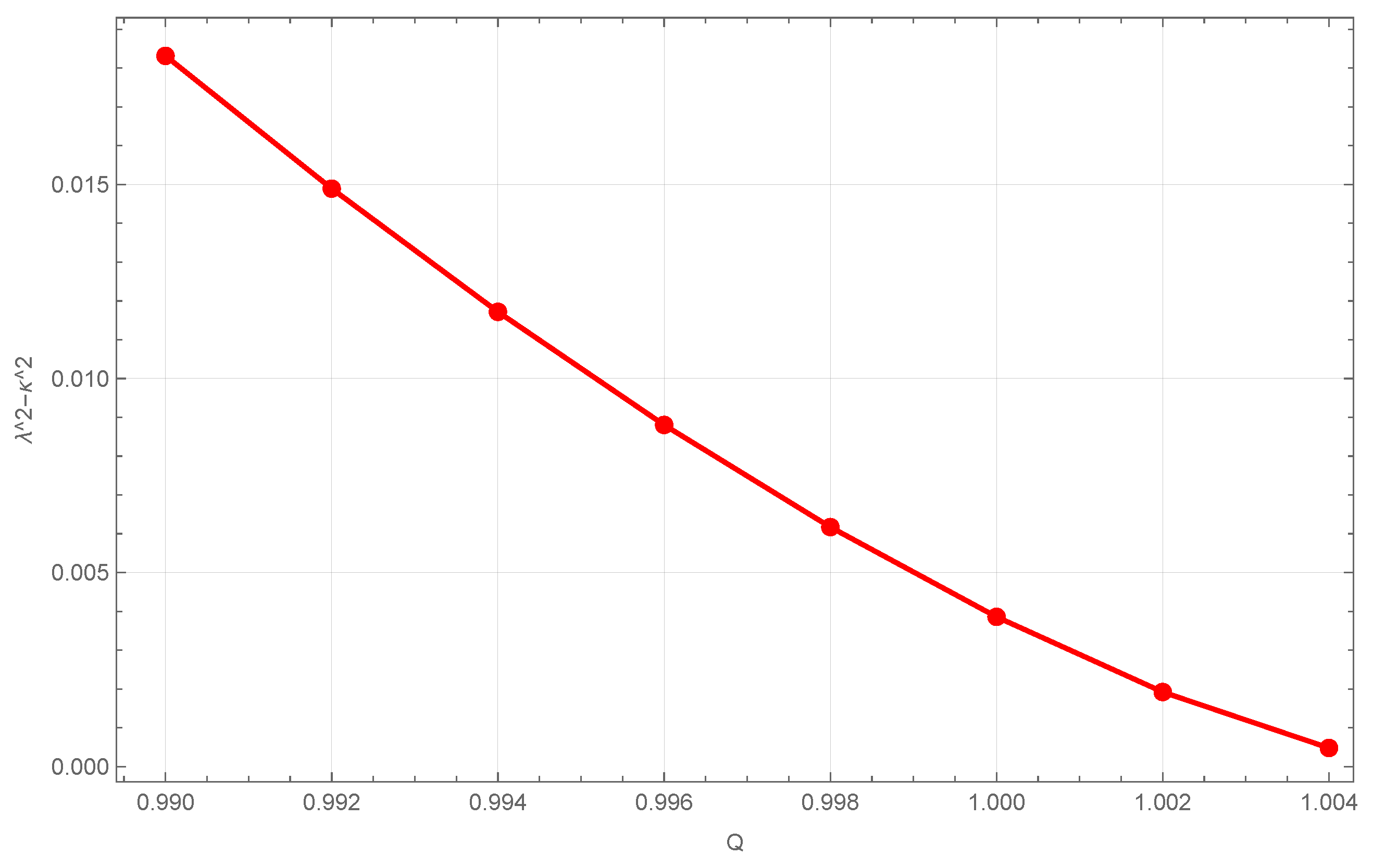
In this section, we investigate the influence of the quantum correction parameter a, the normalization factor c, and the black-hole charge Q on the evolution of string chaos, along with the conditions for violating the MSS bound. The black hole is characterized by Equations (2)–(4), with the event horizon $r_{+}$ defined as the solution to $f\left(r\right)=0$. The surface gravity is given by $\kappa ={\displaystyle \frac{1}{2}}{\left|{\displaystyle \frac{\partial f}{\partial r}}\right|}_{r=r_{+}}$. Using Equation (14), we first calculate the equilibrium orbit radius $r_0$, and then compute the values of the Lyapunov exponent $\lambda$ and the surface gravity $\kappa$. The chaotic dynamics of the string and the violation of the chaos bound are analyzed in Figure 1, Figure 2 and Figure 3. The specific parameter configurations are as follows: Figure 1—$M=1$, $E=14.8$, $c=0.03$, $Q=0.99$, $\theta =0$, and $P_{\theta }=10$; Figure 2—$M=1$, $E=14.8$, $a=0.1$, $Q=0.99$, and $P_{\theta }=10$; and Figure 3—$M=1$, $E=14.8$, $a=0.1$, $c=0.01$, $\theta =0$, and $P_{\theta }=10$. The following phenomena can be observed in these figures.

Figure 1. Effect of parameter a on the MSS bound.

Figure 2. The same as Figure 1, but for parameter c.

Figure 3. The same as Figure 1 and Figure 2, but for Q.

With the energy E, normalization factor c, and charge Q held fixed, different values of the quantum correction parameter a yield different values of ${\lambda }^2-{\kappa }^2$. This quantity is consistently positive, indicating that the system’s chaotic rate exceeds the universal upper bound set by the MSS inequality, signifying an anomalously high chaotic strength. As the parameter a increases, the value of ${\lambda }^2-{\kappa }^2$ also increases. This demonstrates that the violation of the chaotic speed limit becomes more severe, corresponding to a greater degree of anomalous chaotic dynamics.

The normalization factor c influences the MSS bound in a similar manner. Specifically, with other parameters fixed, different values of c also result in distinct ${\lambda }^2-{\kappa }^2$ values. This quantity remains positive and increases with c. The conclusion parallels that of case (1): the system persists in a state of anomalous chaotic intensity, and the value of parameter c modulates the severity of this anomaly and the chaotic rate. A larger c leads to a higher degree of anomalous chaotic dynamics and a faster chaotic rate.

In contrast to the previous parameters, the black-hole charge Q serves to suppress the violation of the MSS bound. For fixed values of the other parameters, an increase in Q causes the value of ${\lambda }^2-{\kappa }^2$ to decrease, although it remains positive. This implies that increasing the charge can mitigate the anomalous chaotic intensity, steering the system dynamics toward the ’normal’ regime constrained by the MSS bound, yet without fully satisfying it. Notably, in Figure 3, ${\lambda }^2-{\kappa }^2$ approaches zero as Q increases. We conjecture that if Q were increased beyond a certain critical charge $Q_c$, a scenario with ${\lambda }^2-{\kappa }^2<0$ might emerge, whereby the system dynamics would comply with the MSS bound. However, our actual calculations show that within the accessible parameter range, the system consistently violates the bound, and the predicted scenario does not occur.

By synthesizing the results from Figure 1, Figure 2 and Figure 3, it becomes evident that the quantum correction parameter a, the normalization factor c, and the black hole’s charge Q significantly influence the system’s chaotic dynamics and the degree of MSS bound violation. Among them, the parameter a exhibits the most pronounced effect in enhancing ${\lambda }^2-{\kappa }^2$ (compare the ordinate scales in Figure 1, Figure 2 and Figure 3). This indicates that quantum correction is the dominant factor in this model responsible for the anomalous chaotic dynamics and the violation of the MSS bound. The condition ${\lambda }^2-{\kappa }^2>0$ in all cases demonstrates that, within the given parameter space, the system cannot satisfy the MSS bound, and its chaotic evolution remains persistently anomalous.

3. The Long-Term Dynamic Evolution of Strings Based on Numerical Methods

3.1. Construction of the Explicit Symplectic Integrators

Building on the analytical investigation of the chaotic dynamics of strings around the black hole and the violation of the MSS bound—which revealed the influence of the quantum correction parameter a, the normalization factor c, and the black hole’s charge Q—this section employs numerical calculations to further examine the impact of these parameters on the system’s chaotic dynamics.

First, an explicit symplectic algorithm for AdS-RN black holes is constructed. In relativistic Hamiltonian systems, the key to constructing explicit symplectic integrators is to require that the Hamiltonian being integrated admits an analytically integrable decomposition—specifically, the analytical solution of each split part must be an explicit function of the proper time $\tau$. However, the Hamiltonian (7) cannot be used to construct an explicit symplectic integrator directly. The reason for this is that the Hamiltonian (7) has two splitting parts: $T={\displaystyle \frac{\pi {\alpha }^{\prime }}{2}}[f\left(r\right)p_r^2+{\displaystyle \frac{p_{\theta }^2}{r^2}}]$ and $V=-{\displaystyle \frac{\pi {\alpha }^{\prime }}{2}}{\displaystyle \frac{E^2}{f\left(r\right)}}+{\displaystyle \frac{1}{2\pi {\alpha }^{\prime }}}{r}^2{\alpha }^2{sin}^2\theta$. The V part is integrable; its analytical solutions are explicit functions of proper time $\tau$. But the T part’s analytical solutions are not [45]. Therefore, it is not possible to construct an explicit symplectic algorithm through two-step decomposition techniques. Consequently, we focus on studying Hamiltonians with more analytically integrable splitting parts using the splitting technique.

We partition the Hamiltonian (7) into eight parts:

$$H=H_1+H_2+H_3+H_4+H_5+H_6+H_7+H_8,$$

(17)

where

$$\begin{array}{cc}\hfill H_1& =-{\displaystyle \frac{E^2}{f\left(r\right)}},\hfill \\ \hfill H_2& ={\displaystyle \frac{\pi {\alpha }^{\prime }}{2}}{\displaystyle \frac{p_{\theta }^2}{r^2}},\hfill \\ \hfill H_3& ={\displaystyle \frac{1}{2\pi {\alpha }^{\prime }}}{r}^2{\alpha }^2{sin}^2\theta ,\hfill \\ \hfill H_4& =-{\displaystyle \frac{\pi {\alpha }^{\prime }{p}_r^2}{2}}{\displaystyle \frac{M}{r}},\hfill \\ \hfill H_5& ={\displaystyle \frac{\pi {\alpha }^{\prime }{p}_r^2}{2}}{\displaystyle \frac{\sqrt{r^2-a^2}}{r}},\hfill \\ \hfill H_6& ={\displaystyle \frac{\pi {\alpha }^{\prime }{p}_r^2}{2}}{\displaystyle \frac{r^2}{{\ell }^2}},\hfill \\ \hfill H_7& =-{\displaystyle \frac{\pi {\alpha }^{\prime }{p}_r^2}{2}}{\displaystyle \frac{c}{r^{3\omega +1}}},\hfill \\ \hfill H_8& ={\displaystyle \frac{\pi {\alpha }^{\prime }}{2}}{\displaystyle \frac{Q^2}{r^2}}.\hfill \end{array}$$

(18)

However, this approach requires that each sub-Hamiltonian system be analytically solvable. For the Hamiltonian in Equation (17), while $H_1-H_4$ and $H_6-H_8$ admit analytical solutions, obtaining an analytical solution for $H_5$ is notably difficult. To address this issue, a time transformation function $d\tau =g\left(r\right)dw$ is introduced, where $\tau$ is the proper time and w is a newly introduced fictitious coordinate time. This method preserves the original dynamics by extending the system into an enlarged phase space. Such an approach forms a foundation for handling time-dependent systems, constrained dynamics, and regularization problems, extending analytical flexibility while preserving physical behavior. Thus, by employing the time transformation function $g\left(r\right)={\displaystyle \frac{1}{r}}$, we extend the phase space and obtain a new Hamiltonian as follows:

$$\mathcal{H}={\displaystyle \frac{1}{r}}(H_1+H_2+H_3+H_4+H_6+H_7+H_8)+{\displaystyle \frac{\pi {\alpha }^{\prime }{p}_r^2}{2}}{\displaystyle \frac{\sqrt{r^2-a^2}}{r^2}},$$

(19)

where $\mathcal{H}$ is limited by the constraint $\mathcal{H}=0$. Due to the presence of the ${\displaystyle \frac{1}{r}}$ term in the new Hamiltonian $\mathcal{H}$, its eighth component has an analytical expression, thereby ensuring the integrability of the entire Hamiltonian $\mathcal{H}$. Thus, the Hamiltonian $\mathcal{H}$ can be further decomposed into the following eight parts:

$$\mathcal{H}={\mathcal{H}}_1+{\mathcal{H}}_2+{\mathcal{H}}_3+{\mathcal{H}}_4+{\mathcal{H}}_5+{\mathcal{H}}_6+{\mathcal{H}}_7+{\mathcal{H}}_8,$$

(20)

Each sub-Hamiltonian can be expressed as follows:

$$\begin{array}{cc}\hfill {\mathcal{H}}_1& =-{\displaystyle \frac{E^2}{rf\left(r\right)}},\hfill \\ \hfill {\mathcal{H}}_2& ={\displaystyle \frac{\pi {\alpha }^{\prime }}{2}}{\displaystyle \frac{p_{\theta }^2}{r^3}},\hfill \\ \hfill {\mathcal{H}}_3& ={\displaystyle \frac{1}{2\pi {\alpha }^{\prime }}}r{\alpha }^2{sin}^2\theta ,\hfill \\ \hfill {\mathcal{H}}_4& =-{\displaystyle \frac{\pi {\alpha }^{\prime }{p}_r^2}{2}}{\displaystyle \frac{M}{r^2}},\hfill \\ \hfill {\mathcal{H}}_5& ={\displaystyle \frac{\pi {\alpha }^{\prime }{p}_r^2}{2}}{\displaystyle \frac{\sqrt{r^2-a^2}}{r^2}},\hfill \\ \hfill {\mathcal{H}}_6& ={\displaystyle \frac{\pi {\alpha }^{\prime }{p}_r^2}{2}}{\displaystyle \frac{r}{{\ell }^2}},\hfill \\ \hfill {\mathcal{H}}_7& =-{\displaystyle \frac{\pi {\alpha }^{\prime }{p}_r^2}{2}}{\displaystyle \frac{c}{r^{3\omega +2}}},\hfill \\ \hfill {\mathcal{H}}_8& ={\displaystyle \frac{\pi {\alpha }^{\prime }}{2}}{\displaystyle \frac{Q^2}{r^3}}.\hfill \end{array}$$

(21)

The canonical equations of the sub-Hamilton are as follows:

$$\begin{array}{cc}\hfill {\mathcal{H}}_1:{\displaystyle \frac{d{P}_r}{dw}}& =-{\displaystyle \frac{\pi {\alpha }^{\prime }{E}^2}{2}}{\displaystyle \frac{[f\left(r\right)+f^{\prime }\left(r\right)r]}{r^2{f}^2\left(r\right)}},\hfill \\ \hfill {\mathcal{H}}_2:{\displaystyle \frac{d\theta }{dw}}& ={\displaystyle \frac{\pi {\alpha }^{\prime }}{2}}{\displaystyle \frac{P_{\theta }}{r^3}},\hfill \\ \hfill {\displaystyle \frac{d{P}_r}{dw}}& ={\displaystyle \frac{3\pi {\alpha }^{\prime }}{2}}{\displaystyle \frac{P_{\theta }^2}{r^4}},\hfill \\ \hfill {\mathcal{H}}_3:{\displaystyle \frac{d{P}_r}{dw}}& =-{\displaystyle \frac{1}{2\pi {\alpha }^{\prime }}}{\alpha }^2{sin}^2\theta ,\hfill \\ \hfill {\displaystyle \frac{d{P}_{\theta }}{dw}}& =-{\displaystyle \frac{1}{\pi {\alpha }^{\prime }}}r{\alpha }^2{sin}^2\theta {cos}^2\theta ,\hfill \\ \hfill {\mathcal{H}}_4:{\displaystyle \frac{dr}{dw}}& =-{\displaystyle \frac{2\pi {\alpha }^{\prime }{P}_{r}M}{r^2}},\hfill \\ \hfill {\displaystyle \frac{d{P}_r}{dw}}& =-{\displaystyle \frac{2\pi {\alpha }^{\prime }{P}_r^{2}M}{r^3}},\hfill \\ \hfill {\mathcal{H}}_5:{\displaystyle \frac{dr}{dw}}& ={\displaystyle \frac{\pi {\alpha }^{\prime }{P}_r\sqrt{r^2-a^2}}{r^2}},\hfill \\ \hfill {\displaystyle \frac{d{P}_r}{dw}}& ={\displaystyle \frac{\pi {\alpha }^{\prime }{P}_r^2(r^2-2a^2)}{2r^3\sqrt{r^2-a^2}}},\hfill \\ \hfill {\mathcal{H}}_6:{\displaystyle \frac{dr}{dw}}& ={\displaystyle \frac{\pi {\alpha }^{\prime }r{P}_r}{{\ell }^2}},\hfill \\ \hfill {\displaystyle \frac{d{P}_r}{dw}}& =-{\displaystyle \frac{\pi {\alpha }^{\prime }{P}_r^2}{2{\ell }^2}},\hfill \\ \hfill {\mathcal{H}}_7:{\displaystyle \frac{dr}{dw}}& =-{\displaystyle \frac{\pi {\alpha }^{\prime }{P}_r}{2}}{\displaystyle \frac{c}{r^{3\omega +2}}},\hfill \\ \hfill {\displaystyle \frac{d{P}_r}{dw}}& =-{\displaystyle \frac{\pi {\alpha }^{\prime }{P}_r^2}{2}}{\displaystyle \frac{c(3\omega +2)}{r^{3\omega +3}}},\hfill \\ \hfill {\mathcal{H}}_8:{\displaystyle \frac{d{P}_r}{dw}}& ={\displaystyle \frac{\pi {\alpha }^{\prime }{P}_{r}Q}{r^3}},\hfill \\ \hfill {\displaystyle \frac{d{P}_r}{dw}}& ={\displaystyle \frac{3\pi {\alpha }^{\prime }{P}_r^{2}Q}{2r^4}}.\hfill \end{array}$$

(22)

The analytical solution to each of these eight split Hamiltonians should be expressed in terms of a new time variable w. Using the given initial conditions ($r_0,P_{r0},{\theta }_0,P_{\theta 0}$), the analytical solution for each part can be written in the following form:

$$\begin{array}{cc}\hfill {\mathcal{H}}_1:& P_r\left(w\right)=P_{r_0}-w{\displaystyle \frac{\pi {\alpha }^{\prime }{E}^2}{2}}{\displaystyle \frac{[f\left(r_0\right)+w{f}^{\prime }\left(r_0\right)r_0]}{r_0^2{f}^2\left(r_0\right)}},\hfill \\ \hfill {\mathcal{H}}_2:& \theta \left(w\right)={\theta }_0+w{\displaystyle \frac{\pi {\alpha }^{\prime }}{2}}{\displaystyle \frac{P_{\theta 0}}{r_0^3}},\hfill \\ \hfill & P_r\left(w\right)=P_{r_0}+w{\displaystyle \frac{3\pi {\alpha }^{\prime }}{2}}{\displaystyle \frac{P_{\theta 0}^2}{r_0^4}},\hfill \\ \hfill {\mathcal{H}}_3:& P_r\left(w\right)=P_{r0}-{\displaystyle \frac{w}{2\pi {\alpha }^{\prime }}}{\alpha }^2{sin}^2{\theta }_0,\hfill \\ \hfill & P_{\theta }\left(w\right)=P_{\theta 0}-{\displaystyle \frac{w}{\pi {\alpha }^{\prime }}}{r}_0{\alpha }^2{sin}^2{\theta }_0{cos}^2{\theta }_0,\hfill \\ \hfill {\mathcal{H}}_4:& r\left(w\right)=\sqrt{r_0^2-{\displaystyle \frac{4M\pi {\alpha }^{\prime }{P}_{r0}w}{r_0}}},\hfill \\ \hfill & P_r\left(w\right)=P_{r0}\sqrt{1-{\displaystyle \frac{4M\pi {\alpha }^{\prime }{P}_{r0}w}{r_0^3}}},\hfill \\ \hfill {\mathcal{H}}_5:& r\left(w\right)=\sqrt{a^2+(r_0^2-a^2){(1+Fw)}^{\frac{4}{3}}},\hfill \\ \hfill & P_r\left(w\right)=P_{r0}r\left(w\right){\displaystyle \frac{(1+Fw)}{r_0}},\hfill \\ \hfill {\mathcal{H}}_6:& r\left(w\right)=r_0{(1+{\displaystyle \frac{\pi {\alpha }^{\prime }{P}_{r}w}{2{\ell }^2}})}^2,\hfill \\ \hfill & P_r\left(w\right)={\displaystyle \frac{2{\ell }^2{P}_{r0}}{w\pi {\alpha }^{\prime }{P}_{r0}+2{\ell }^2}},\hfill \\ \hfill {\mathcal{H}}_7:& r\left(w\right)={[r_0^{\frac{3\omega +4}{2}}-{\displaystyle \frac{c\pi {\alpha }^{\prime }{P}_{r0}(3\omega +4)w}{2r_0^{\frac{3\omega +2}{2}}}}]}^{\frac{2}{3\omega +4}},\hfill \\ \hfill & P_r\left(w\right)=P_{r0}{({\displaystyle \frac{r\left(w\right)}{r_0}})}^{\frac{3\omega +2}{2}},\hfill \\ \hfill {\mathcal{H}}_8:& r\left(w\right)=r_0{(1+{\displaystyle \frac{5Q^2\pi {\alpha }^{\prime }{P}_{r0}w}{2r_0^4}})}^{\frac{2}{5}},\hfill \\ \hfill & P_r\left(w\right)=P_{r0}{(1+{\displaystyle \frac{5Q^2\pi {\alpha }^{\prime }{P}_{r0}w}{2r_0^4}})}^{\frac{3}{5}},\hfill \end{array}$$

(23)

where $F={\displaystyle \frac{3\pi {\alpha }^{\prime }{P}_{r0}}{2r_0\sqrt{r_0^2-a^2}}}$, and $f^{\prime }$ denotes the derivative of f with respect to r.

Next, we construct a second-order explicit symplectic integrator $S_2$ with a fixed time step h, given by the symmetric composition of operators $S_2\left(h\right)$ = ${\mathcal{X}}_{\frac{h}{2}}\circ {{\mathcal{X}}^{\ast }}_{\frac{h}{2}}$, where

$${\mathcal{X}}_h={\mathcal{H}}_8\left(h\right)\circ {\mathcal{H}}_7\left(h\right)\circ {\mathcal{H}}_6\left(h\right)\circ {\mathcal{H}}_5\left(h\right)\circ {\mathcal{H}}_4\left(h\right)\circ {\mathcal{H}}_3\left(h\right)\circ {\mathcal{H}}_2\left(h\right)\circ {\mathcal{H}}_1\left(h\right)$$

(24)

$${{\mathcal{X}}^{\ast }}_h={\mathcal{H}}_1\left(h\right)\circ {\mathcal{H}}_2\left(h\right)\circ {\mathcal{H}}_3\left(h\right)\circ {\mathcal{H}}_4\left(h\right)\circ {\mathcal{H}}_5\left(h\right)\circ {\mathcal{H}}_6\left(h\right)\circ {\mathcal{H}}_7\left(h\right)\circ {\mathcal{H}}_8\left(h\right)$$

(25)

Here, ${\mathcal{X}}_h$ and ${{\mathcal{X}}^{\ast }}_h$ are approximate evolution operators formed by a single combination of the exact evolution operators for the eight decomposed sub-Hamiltonian systems [48]. By applying the composition scheme proposed by Yoshida [77], the accuracy of the algorithm can be raised to the fourth order:

$$S_4=S_2\left(\gamma h\right)\circ S_2\left(\beta h\right)\circ S_2\left(\gamma h\right),$$

where $\gamma =1/(2-{\displaystyle \sqrt[3]{2}})$, and $\beta =1-2\gamma$.

This high-order scheme reduces the global truncation error by eliminating lower-order error terms, making it suitable for high-precision numerical simulations over medium to long time scales.

3.2. Dynamics of Strings

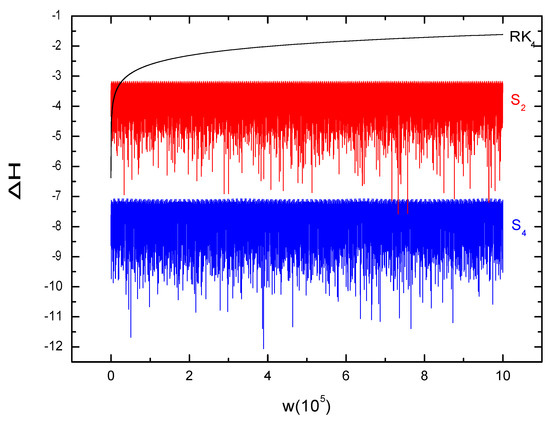
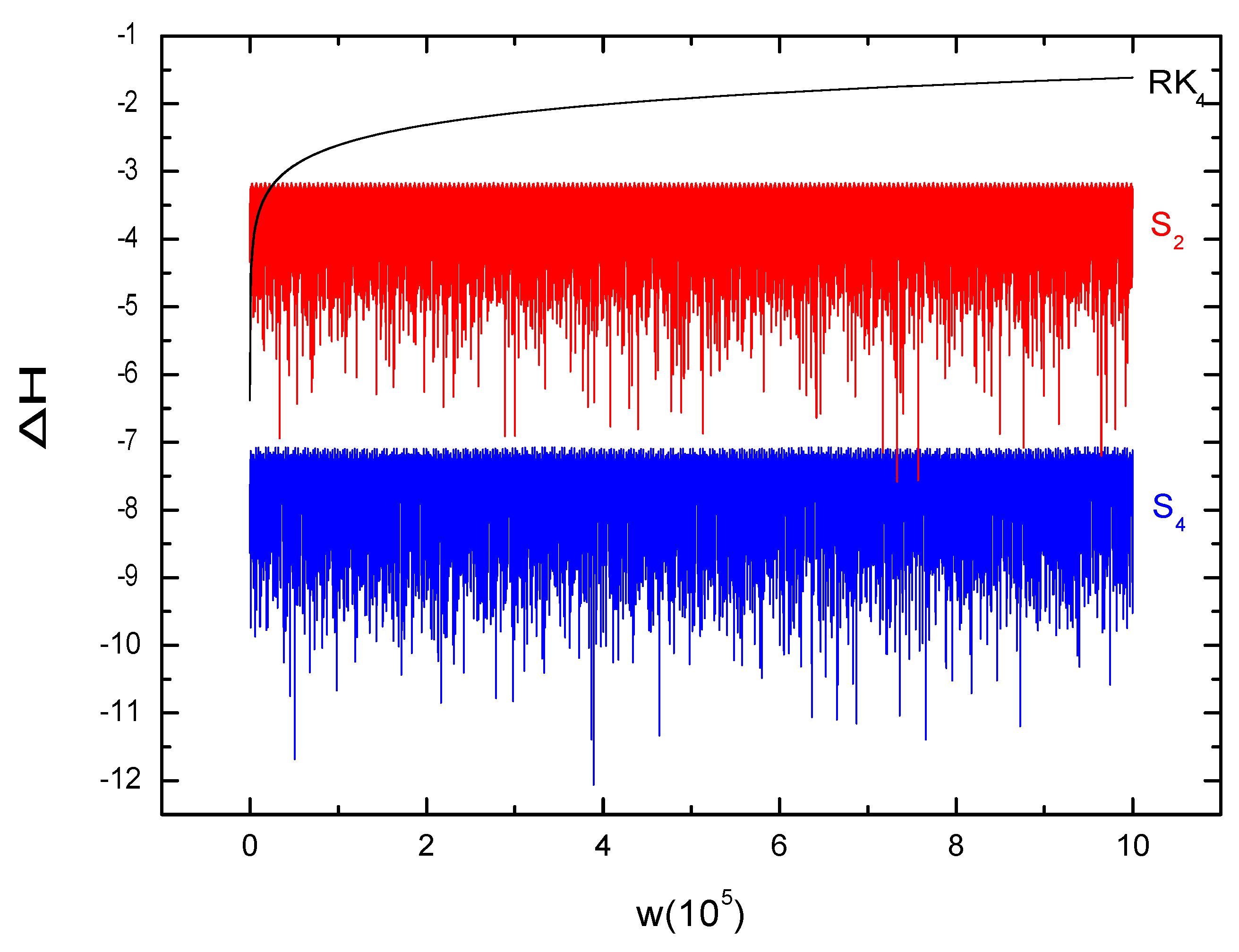
To demonstrate the performance of symplectic integrators, the traditional fourth-order Runge–Kutta integrator ($R{K}_4$), a second-order symplectic integrator ($S_2$), and a fourth-order symplectic integrator ($S_4$) are used for comparison. The parameters were set as follows: $M=1,E=14.8,c=0.01,a=0.1,Q=2.8,r=7,\theta ={\displaystyle \frac{\pi }{4}},P_r=0.01,\alpha =1,{\alpha }^{\prime }={\displaystyle \frac{1}{\pi }}$, and $P_{\theta }$ was obtained from Equation (19). The time step was set to $h=0.02$, and the integration time is ${10}^5$. As shown in Figure 4, which presents the Hamiltonian errors produced by the algorithms $S_2$, $S_4$, and $RK4$, the errors from $S_2$ and $S_4$ are bounded and stable, with $S_4$ exhibiting smaller errors. In contrast, the error from $R{K}_4$ increases linearly with time and is significantly larger. This result is consistent with theoretical expectations, as $R{K}_4$ is not a geometric integrator. After the error characteristics of different integrators were verified through numerical simulations, the advantage of the $S_4$ algorithm in maintaining long-term system stability was confirmed. Subsequently, to study the chaotic behavior of the system, orbit calculations will be performed based on $S_4$, and the identification of chaos will rely on a series of quantitative indicators.

Figure 4. The Hamiltonian error $\Delta$H generated by the fourth-order Runge–Kutta ($R{K}_4$), second-order symplectic ($S_2$), and fourth-order symplectic algorithms $S_4$. Here, the initial parameters are $E=14.8$, $a=0.1$, $c=0.01$, $Q=2.8,r=7,\theta ={\displaystyle \frac{\pi }{4}},P_r=0.01$, and $P_{\theta }$ obtained from Equation (19).

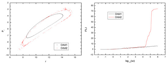
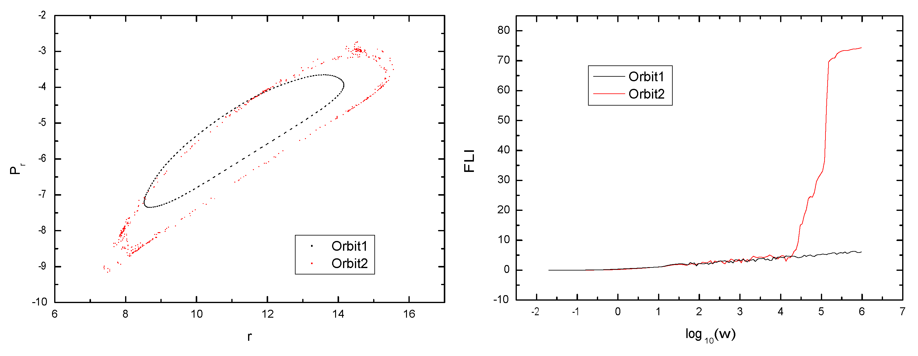
Many chaos indicators have been proposed in the literature, such as the Poincaré section method, Lyapunov exponents, the Fast Lyapunov Indicator (FLI), and spectral analysis. Studies have shown that Poincaré sections and the FLI are straightforward and easy to implement [13,41]. For instance, the initial parameters for orbit 1 can be set to $E=14.5,a=0.1,c=0.01,Q=2.7,r=7,$$\theta ={\displaystyle \frac{\pi }{4}},and{P}_r=0.01$, and $P_{\theta }$ can subsequently be derived from Equation (19), and those for orbit 2 can likewise be set to $E=14.95,$$a=0.5,c=0.01,Q=2.8,r=8,$$\theta ={\displaystyle \frac{\pi }{4}},P_r=0.125$, and $P_{\theta }$ from Equation (19). The results are shown in the left plane of Figure 5. Orbit 1 forms a closed, regular curve, indicating ordered motion, whereas the points associated with orbit 2 are randomly scattered, demonstrating chaotic behavior. The FLI is a widely used chaos indicator. It overcomes the limitations of Poincaré sections in three-dimensional dynamical systems. Moreover, compared to other indicators, the FLI is faster, more sensitive, and more accurate in distinguishing between ordered and chaotic orbits. Using the method of employing two nearby orbits, we obtain the FLI, as shown in the right plane of Figure 5. For the ordered orbit 1, the FLI grows linearly with time, whereas for the chaotic orbit 2, it grows exponentially. By comparing the two subfigures in Figure 5, it can be seen that the conclusions drawn from the Poincaré section can be validated with the FLI—if the Poincaré section of an orbit indicates chaos, its FLI will grow exponentially; if the Poincaré section shows order, the corresponding FLI will grow linearly. Therefore, to more intuitively identify chaotic orbits, the FLI will be used for chaos detection in the following analysis. Additionally, the effects of the quantum correction parameter a, the normalization factor c, and the black hole’s charge Q on string dynamics will be discussed. Based on the numerical results depicting the variation in the FLI with the parameters, as shown in Figure 6, Figure 7 and Figure 8, we have the following findings:

Figure 5. The Poincaré sections (the left plane) and FLIs (the right plane) for the two orbits. For orbit 1, the parameters are $E=14.5,a=0.1,c=0.01,Q=2.7,r=7,\theta ={\displaystyle \frac{\pi }{4}},and{P}_r=0.01$. For orbit 2, the parameters are $E=14.95,a=0.5,c=0.01,Q=2.8,r=8,\theta ={\displaystyle \frac{\pi }{4}},and{P}_r=0.125$. Here, $P_{\theta }$ is derived from Equation (19).

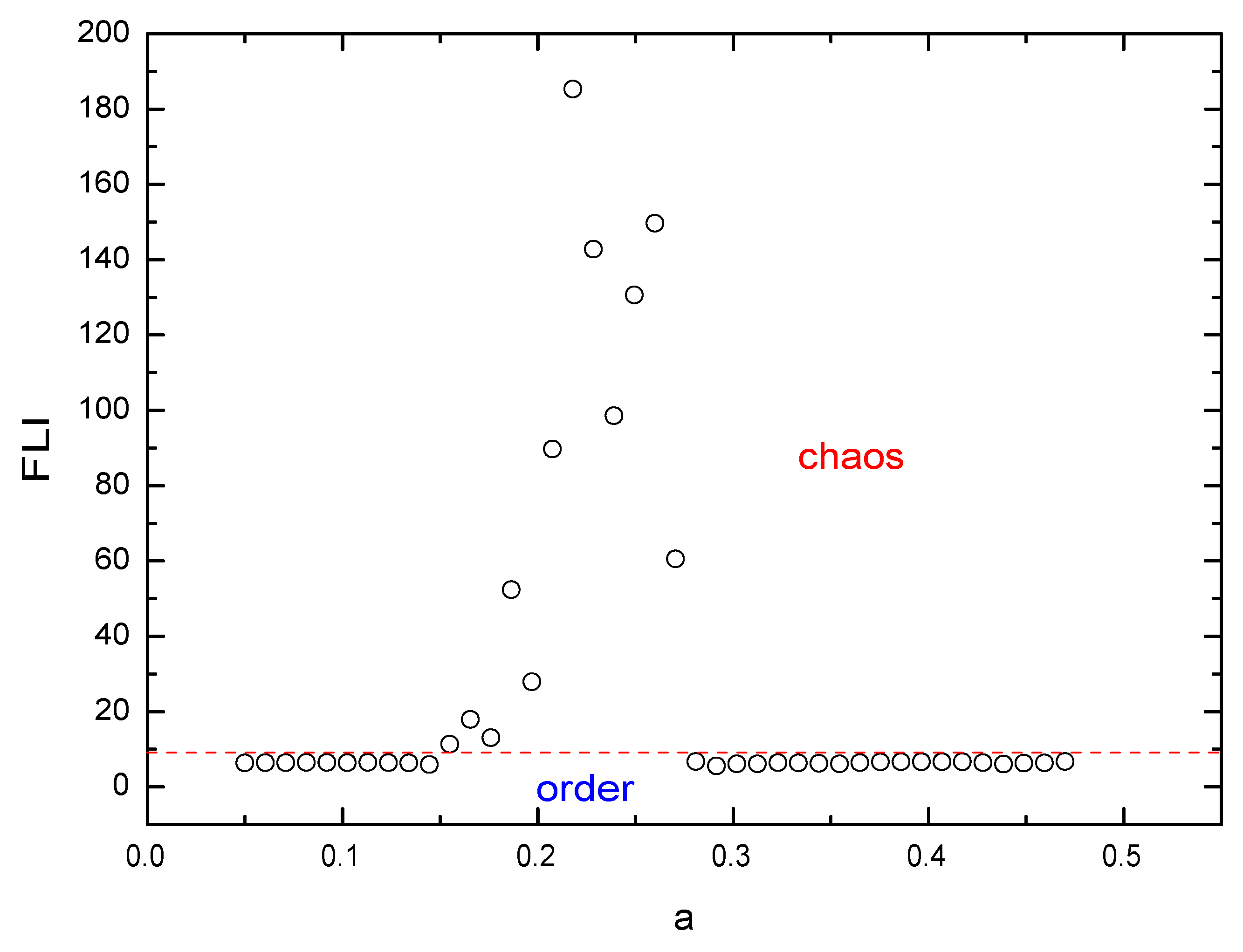
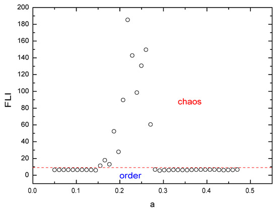
Figure 6. Variation in the FLIs with the quantum correction parameter a. Here, the integration time is ${10}^6$, and the red dash line represents FLI = 9.

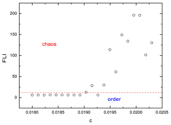
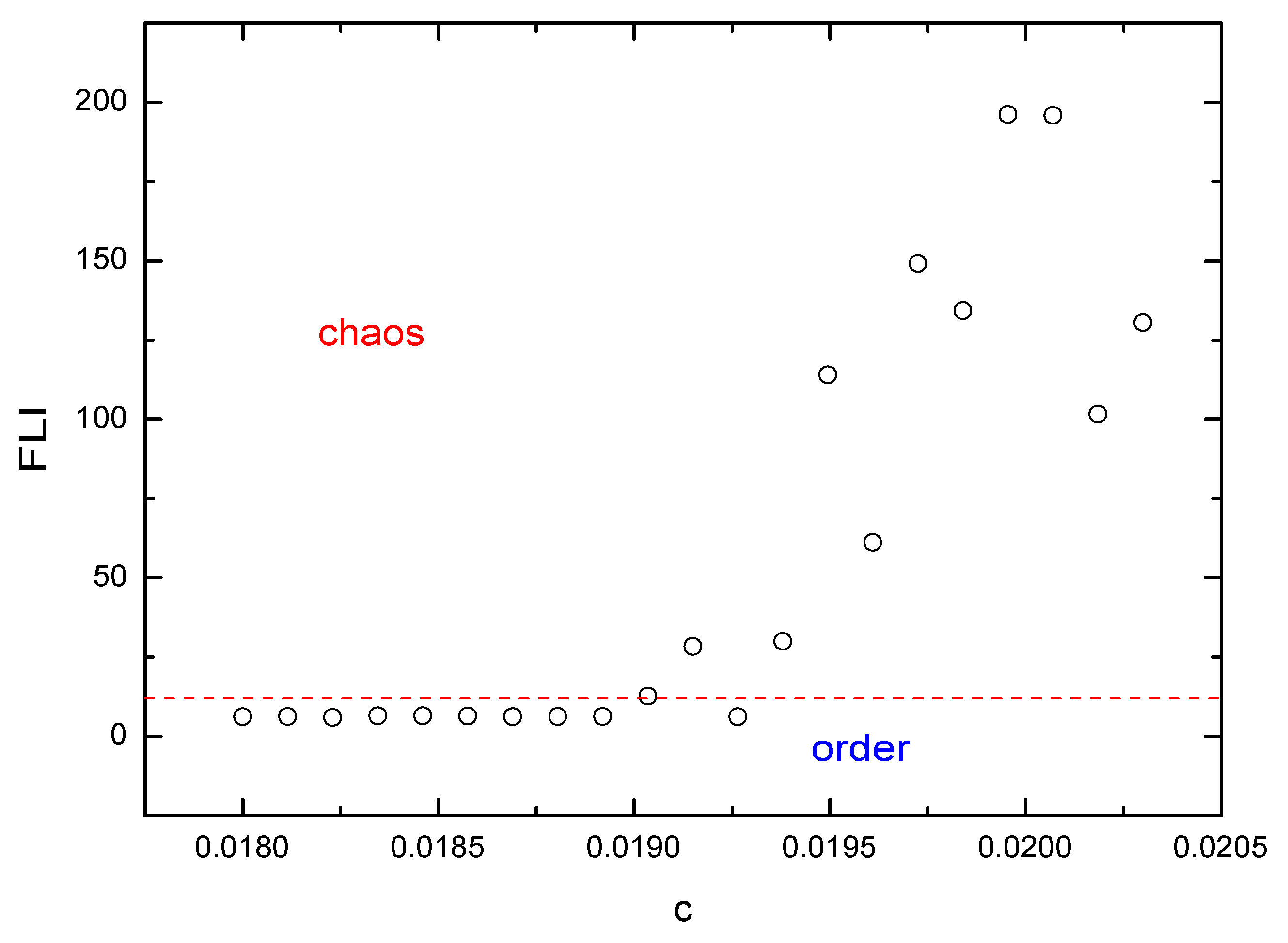
Figure 7. FLI versus the normalization factor c. Here, the integration time and the red dash line are the same as Figure 6.

Figure 8. Variation in the FLI as the black hole’s charge Q changes. Here, the integration time is the same as Figure 6 and Figure 7, but the red dashed line indicating FLI = 15.

The dependence of the FLI on the quantum correction parameter a is shown in Figure 6. The parameters were set as follows: $M=1,E=14.8,Q=2.75,r=7,\theta ={\displaystyle \frac{\pi }{4}},P_r=0.01$, $\alpha =1,{\alpha }^{\prime }={\displaystyle \frac{1}{\pi }}$, and $c=0.02$. Each point in the figure represents an orbit under a different value of a. The FLI is computed for 41 orbits, with the threshold FLI = 9 (indicated by the red dashed line in the figure) used to distinguish between chaotic and ordered orbits: FLI ≥ 9 corresponds to chaotic orbits, while FLI < 9 corresponds to ordered ones.

In Figure 6, it can be observed that when $0.05\le a\le 0.1445$, the system remains in an ordered state. Once a exceeds 0.155, the FLI increases abruptly, indicating that the system begins to transition from order to chaos as a increases. The FLI reaches its maximum at $a=0.218$, suggesting that within this interval, the chaotic behavior strengthens with an increasing a. Subsequently, in the $0.218<a\le 0.2705$ range, the FLI continues to decrease, implying a gradual weakening of chaos, though the system remains chaotic. When a exceeds 0.281, the FLI drops sharply below 9, meaning that once a surpasses this threshold, the system returns to an ordered state. Overall, as the parameter a increases, the system exhibits an evolutionary pattern of “order to chaos to order”.

The variation in the FLI with the normalization factor c is shown in Figure 7, with the parameters set as follows: $M=1,E=14.8,Q=2.747,r=7,\theta ={\displaystyle \frac{\pi }{4}},P_r=0.01,\alpha =1,{\alpha }^{\prime }={\displaystyle \frac{1}{\pi }}$, and $a=0.15$. The FLI was computed for 21 different orbits, and the same criterion as before was adopted: an FLI ≥ 9 indicates chaotic orbits, while an FLI < 9 indicates ordered ones.

As can be seen from Figure 7, the system remains ordered when $c\le 0.01892$. For $c>0.01938$, the system enters a chaotic state, with chaos strengthening as c increases. Within the narrow interval of $0.01892<c<0.01938$, the dynamical behavior of the system is more complex. Specifically, chaos is observed in the $0.01892<c\le 0.01915$ range, whereas in the $0.01927\le c<0.01938$ sub-range, the system transitions from chaos back to order. Overall, as the normalization factor c increases, the system tends to shift from order to chaos.

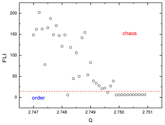
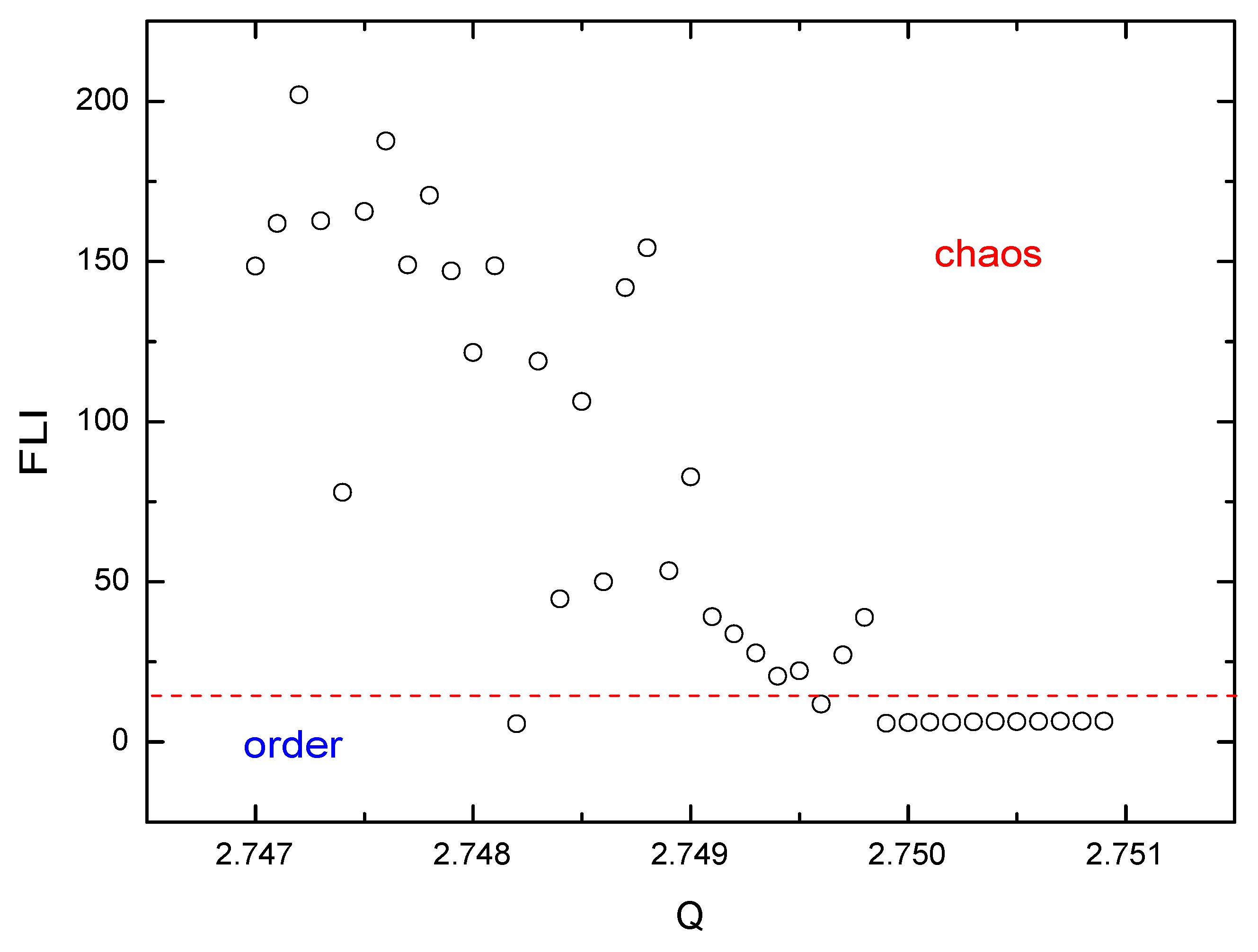
Finally, we examine the influence of black-hole charge Q on the FLI. The parameters are set as follows: $M=1,E=14.8,c=0.02,r=7,\theta ={\displaystyle \frac{\pi }{4}},P_r=0.01,\alpha =1,{\alpha }^{\prime }={\displaystyle \frac{1}{\pi }}$, and $a=0.15$. The FLI is computed for 41 different orbits, with an FLI ≥ 15 and an FLI < 15 used to distinguish chaotic orbits from ordered ones, respectively.

Based on Figure 8, it can be concluded that the overall chaotic behavior of the system weakens as Q decreases. When Q falls below a certain threshold (approximately $Q=2.7499$), the system transitions to an ordered state; in other words, a smaller charge tends to suppress chaos. Notably, while the system is generally chaotic in the $2.7475\le Q\le 2.7498$ range, ordered behavior emerges in two sub-intervals: $2.7481<Q<2.7483$ and $2.7495<Q<2.7497$.

In summary, we find that the chaotic dynamics of the string are significantly influenced by the quantum correction parameter a, the normalization factor c, and the black hole’s charge Q. As the parameter a increases, the system exhibits a transition from order to chaos and back to order. An increase in the normalization factor c drives the system from an ordered state into chaos. Conversely, an increase in black-hole charge Q suppresses chaotic behavior, causing the system to transition from chaos to order.

Our previous research demonstrated that, near the event horizon of an anti-de Sitter Gauss–Bonnet black hole, the chaotic motion of strings is more intense than that of particles, and the degree of chaos strengthens with an increasing Gauss–Bonnet parameter [12]. Moreover, for charged black branes featuring hyperscaling violation (HV), numerical simulations indicate that the chaotic dynamics are collectively influenced by the Hawking temperature, the Lifshitz dynamical exponent, and the HV exponent [13]. Additionally, a study of string chaos around a conformal black hole revealed that its characteristic parameter plays a crucial role in determining chaotic behavior, and a notable transition occurs when the black-hole horizon vanishes [14]. The present results thus provide an important complement to our understanding of string dynamics around charged black holes.

4. Conclusions

In this study, we employed both analytical and numerical methods to investigate the chaotic motion of strings near a quantum-corrected AdS-RN black hole in Kiselev spacetime. Analytically, we derived the Lyapunov exponent of the string dynamics and examined how parameter variations affect the violation of the MSS bound. The results show that the quantum-correction parameter a, the normalization factor c, and black-hole charge Q all influence the magnitude of the Lyapunov exponent $\lambda$ and play a significant role in violating the chaos bound. All three parameters can drive the system to exceed the MSS bound, with a having the most pronounced effect. Variations in a lead to a more severe anomalous chaotic state. Numerically, we transformed the original Hamiltonian via a time-transformation function, split it into eight integrable parts, and constructed a symplectic algorithm to study the chaotic string dynamics. Numerical experiments demonstrated that the $S_4$ algorithm offers the highest accuracy, with notable advantages in stability and precision for long-term integration. Using $S_4$, we computed the FLI and systematically examined the influence of a, c, and Q on chaos. The results indicate that as a increases, the system undergoes an “order–chaos–order” transition; as c increases, it transitions from order to chaos; and as Q increases, it shifts from chaos to order. The findings of this work provide a deeper understanding of string dynamics under quantum corrections and provide a new perspective for analyzing chaotic motion in strong gravitational fields.

References

- Dettmann, C.P.; Frankel, N.E.; Cornish, N.J. Fractal basins and chaotic trajectories in multi-black hole spacetimes. Phys. Rev. D 1994, 50, R618–R621. [Google Scholar] [CrossRef] [Scilit]
- Santoprete, M.; Cicogna, G. Chaos in Black Holes Surrounded by Electromagnetic Fields. Gen. Relativ. Gravit. 2002, 34, 1107–1119. [Google Scholar] [CrossRef] [Scilit]
- Basu, P.; Chaturvedi, P.; Samantray, P. Chaotic dynamics of strings in charged black hole backgrounds. Phys. Rev. D 2017, 95, 066014. [Google Scholar] [CrossRef] [Scilit]
- Levin, J.; Perez-Giz, G. A Periodic Table for Black Hole Orbits. Phys. Rev. D 2008, 77, 103005. [Google Scholar] [CrossRef] [Scilit]
- Cardoso, V.; Miranda, A.S.; Berti, E.; Witek, H.; Zanchin, V.T. Geodesic stability, Lyapunov exponents, and quasinormal modes. Phys. Rev. D 2009, 79, 064016. [Google Scholar] [CrossRef] [Scilit]
- Maldacena, J.; Shenker, S.H.; Stanford, D. A bound on chaos. J. High Energy Phys. 2016, 8, 106. [Google Scholar] [CrossRef] [Scilit]
- Gao, C.; Chen, D.; Yu, C.; Wang, P. Chaos bound and its violation in charged Kiselev black hole. Phys. Lett. B 2022, 833, 137343. [Google Scholar] [CrossRef] [Scilit]
- Chen, S.; Wang, M.; Jing, J. Chaotic motion of particles in the accelerating and rotating black hole spacetime. J. High Energ Phys. 2016, 9, 082. [Google Scholar] [CrossRef] [Scilit]
- Wang, M.; Chen, S.; Jing, J. Chaotic shadow of a non-Kerr rotating compact object with quadrupole mass moment. Phys. Rev. D 2018, 98, 104040. [Google Scholar] [CrossRef] [Scilit]
- Suzuki, S.; Maeda, K.i. Chaos in Schwarzschild spacetime: The motion of a spinning particle. Phys. Rev. D 1997, 55, 4848–4859. [Google Scholar] [CrossRef] [Scilit]
- Levin, J. Chaos and order in models of black hole pairs. Phys. Rev. D 2006, 74, 124027. [Google Scholar] [CrossRef] [Scilit]
- Ma, D.Z.; Wu, J.P.; Zhang, J.F. Chaos from the ring string in Gauss-Bonnet black hole in AdS5 space. Phys. Rev. D 2014, 89, 086011. [Google Scholar] [CrossRef] [Scilit]
- Ma, D.Z.; Zhang, D.; Fu, G.Y.; Wu, J.P. Chaotic dynamics of string around charged black brane with hyperscaling violation. J. High Energ Phys. 2020, 1, 103. [Google Scholar] [CrossRef] [Scilit]
- Ma, D.Z.; Xia, F.; Zhang, D.; Fu, G.Y.; Wu, J.P. Chaotic dynamics of string around the conformal black hole. Eur. Phys. J. C 2022, 82, 372. [Google Scholar] [CrossRef] [Scilit]
- Li, K.; Ma, D.-Z.; Xu, Z.-M. Chaotic dynamics of string around the charged Kiselev black hole. Phys. Lett. B 2025, 860, 139164. [Google Scholar] [CrossRef] [Scilit]
- Chen, D.; Gao, C. Angular momentum and chaos bound of charged particles around Einstein–Euler–Heisenberg AdS black holes. New J. Phys. 2022, 24, 123014. [Google Scholar] [CrossRef] [Scilit]
- Chen, D.; Yang, C.; Liu, Y. Lyapunov exponents as probes for a phase transition of a Kerr-AdS black hole. Phys. Lett. B 2025, 865, 139463. [Google Scholar] [CrossRef] [Scilit]
- He, Y.; Wang, Z.; Chen, D. Report on chaos bound outside Taub-NUT black holes. Phys. Dark Universe 2023, 42, 101325. [Google Scholar] [CrossRef] [Scilit]
- Chen, D.; Tao, J.; Yang, X. Attractive interactions in the microstructures of asymptotically flat black holes. Phys. Dark Universe 2023, 42, 101379. [Google Scholar] [CrossRef] [Scilit]
- Suzuki, S.; Maeda, K.i. Signature of chaos in gravitational waves from a spinning particle. Phys. Rev. D 2000, 61, 024005. [Google Scholar] [CrossRef] [Scilit]
- Szybka, S.J.; Naqvi, S.U. Chaos and Einstein-Rosen gravitational waves. Phys. Rev. D 2023, 108, L081501. [Google Scholar] [CrossRef] [Scilit]
- Mishra, B.; Kluźniak, W.; Fragile, P.C. Breathing oscillations in a global simulation of a thin accretion disc. Mon. Not. R. Astron. Soc. 2019, 483, 4811–4819. [Google Scholar] [CrossRef] [Scilit]
- Karak, B.B.; Dutta, J.; Mukhopadhyay, B. Search for chaos in neutron star systems: Is Cyg X-3 a black hole? Astrophys. J. 2009, 708, 862–867. [Google Scholar] [CrossRef] [Scilit]
- Gwak, B.; Kan, N.; Lee, B.h.; Lee, H. Violation of bound on chaos for charged probe in Kerr-Newman-AdS black hole. J. High Energy Phys. 2022, 9, 026. [Google Scholar] [CrossRef] [Scilit]
- Frolov, A.V.; Larsen, A.L. Chaotic scattering and capture of strings by a black hole. Class. Quantum Gravity 1999, 16, 3717–3724. [Google Scholar] [CrossRef] [Scilit]
- Carter, B. Global structure of the Kerr family of gravitational fields. Phys. Rev. 1968, 174, 1559. [Google Scholar] [CrossRef] [Scilit]
- Dutta, P.; Panigrahi, K.L.; Singh, B. Circular string in a black p-brane leading to chaos. J. High Energy Phys. 2023, 10, 189. [Google Scholar] [CrossRef] [Scilit]
- Shukla, B.; Riyaz, O.; Mahapatra, S. Classical and quantum chaos of closed strings on a charged confining holographic background. Phys. Rev. D 2025, 111, 066019. [Google Scholar] [CrossRef] [Scilit]
- Dutta, P.; Panigrahi, K.L.; Singh, B. Chaos bound and its violation in black p-brane. J. High Energy Phys. 2025, 2, 043. [Google Scholar] [CrossRef] [Scilit]
- Colangelo, P.; Giannuzzi, F.; Losacco, N. Chaotic dynamics of a suspended string in a gravitational background with magnetic field. Phys. Lett. B 2022, 827, 136949. [Google Scholar] [CrossRef] [Scilit]
- Ishii, T.; Kushiro, S.; Yoshida, K. Chaotic string dynamics in deformed T1,1. J. High Energy Phys. 2021, 5, 158. [Google Scholar] [CrossRef] [Scilit]
- Zhao, Q.Q.; Li, Y.; Lu, H.Q. Static equilibria of charged particles around charged black holes: Chaos bound and its violations. Phys. Rev. D 2022, 98, 124001. [Google Scholar] [CrossRef] [Scilit]
- Kan, N.; Gwak, B. Bound on the Lyapunov exponent in Kerr-Newman black holes via a charged particle. Phys. Rev. D 2022, 105, 026006. [Google Scholar] [CrossRef] [Scilit]
- Kazakov, D.I.; Solodukhin, S.N. On quantum deformation of the Schwarzschild solution. Nucl. Phys. B. 1994, 429, 153–176. [Google Scholar] [CrossRef] [Scilit]
- Bezerra, V.B.; Lobo, I.P.; Graça, J.P.M.; Santos, L.C.N. Effects of quantum corrections on the criticality and eficiency of black holes surrounded by a perfect uid. Eur. Phys. J. C 2019, 79, 949. [Google Scholar] [CrossRef] [Scilit]
- Shahjalal, M. Thermodynamics of quantum-corrected Schwarzschild black hole surrounded by quintessence. Nucl. Phys. B. 2019, 940, 63–77. [Google Scholar] [CrossRef] [Scilit]
- Nozari, K.; Hajebrahimi, M.; Saghafi, S. Quantum corrections to the accretion onto a Schwarzschild black hole in the background of quintessence. Eur. Phys. J. C 2020, 80, 1208. [Google Scholar] [CrossRef] [Scilit]
- Konoplya, R.A. Quantum corrected black holes: Quasinormal modes, scattering, shadows. Phys. Lett. B 2020, 804, 135363. [Google Scholar] [CrossRef] [Scilit]
- Graça, J.P.M.; Capossoli, E.F.; Boschi-Filho, H.; Lobo, I.P. Joule-Thomson expansion for quantum corrected AdS-Reissner-Nordström black holes in a Kiselev spacetime. Phys. Rev. D 2023, 107, 024045. [Google Scholar] [CrossRef] [Scilit]
- Sadeghi, J.; Gashti, S.N.; Alipour, M.R.; Afshar, M.A.S. Thermodynamic topology of quantum corrected AdS-Reissner-Nordstrom black holes in Kiselev spacetime. Chin. Phys. C. 2024, 48, 115115. [Google Scholar] [CrossRef] [Scilit]
- Ma, D.Z.; Wu, X.; Zhu, J.F. Velocity Scaling Method to Correct Individual Kepler Energies. New Astron. 2008, 13, 216–223. [Google Scholar] [CrossRef] [Scilit]
- Sanz-Serna, J.M. Symplectic integrators for Hamiltonian problems: An overview. Acta Numer. 1992, 1, 243–286. [Google Scholar] [CrossRef] [Scilit]
- Marsden, J.E.; West, M. Discrete mechanics and variational integrators. Acta Numer. 2001, 10, 357–514. [Google Scholar] [CrossRef] [Scilit]
- Wu, X.; Wang, Y.; Sun, W.; Liu, F.Y.; Ma, D.Z. Explicit Symplectic Integrators with Adaptive Time Steps in Curved Spacetimes. Astrophys. J. Suppl. 2024, 275, 31. [Google Scholar] [CrossRef] [Scilit]
- Wang, Y.; Sun, W.; Liu, F.Y.; Wu, X. Construction of Explicit Symplectic Integrators in General Relativity. I. Schwarzschild Black Holes. Astrophys. J. 2021, 907, 66. [Google Scholar] [CrossRef] [Scilit]
- Wang, Y.; Sun, W.; Liu, F.Y.; Wu, X. Construction of Explicit Symplectic Integrators in General Relativity. II. Reissner–Nordström Black Holes. Astrophys. J. 2021, 909, 22. [Google Scholar] [CrossRef] [Scilit]
- Wang, Y.; Sun, W.; Liu, F.Y.; Wu, X. Construction of Explicit Symplectic Integrators in General Relativity. III. Reissner–Nordström–(anti)-de Sitter Black Holes. Astrophys. J. Suppl. 2021, 254, 8. [Google Scholar] [CrossRef] [Scilit]
- Wu, X.; Wang, Y.; Sun, W.; Liu, F.Y. Construction of Explicit Symplectic Integrators in General Relativity. IV. Kerr Black Holes. Astrophys. J. 2021, 914, 63. [Google Scholar] [CrossRef] [Scilit]
- Mikkola, S. Practical Symplectic Methods with Time Transformation for the Few-body Problem. Celest. Mech. Dyn. Astron. 1997, 67, 145–165. [Google Scholar] [CrossRef] [Scilit]
- Hu, A.R.; Huang, G.Q. Chaos in a Magnetized Brane-world Space-time Using Explicit Symplectic Integrators. Universe 2022, 8, 369. [Google Scholar] [CrossRef] [Scilit]
- Sanz-Serna, J.M.; Calvo, M.P. Numerical Hamiltonian Problems; Chapman & Hall: London, UK, 1994; Volume 7. [Google Scholar]
- Feng, K. On difference schemes and symplectic geometry. In Proceedings of the 5th International Symposium on Differential Geometry and Differential Equations; Science Press: Beijing, China, 1985; pp. 42–58. [Google Scholar]
- Ruth, R.D. A Canonical Integration Technique. IEEE Trans. Nucl. Sci. 1983, 30, 2669–2671. [Google Scholar] [CrossRef] [Scilit]
- Pánis, R.; Kološ, M.; Stuchlík, Z. Determination of chaotic behaviour in time series generated by charged particle motion around magnetized Schwarzschild black holes. Eur. Phys. J. C 2019, 79, 479. [Google Scholar] [CrossRef] [Scilit]
- Hanan, W.; Radu, E. Chaotic motion in multi-black hole spacetimes and holographic screens. Mod. Phys. Lett. A 2007, 22, 399–406. [Google Scholar] [CrossRef] [Scilit]
- Karas, V.; Vokrouhlický, D. Chaotic motion of test particles in the Ernst space-time. Gen. Rel. Grav. 1992, 24, 729–743. [Google Scholar] [CrossRef] [Scilit]
- Johannsen, T.; Psaltis, D. A Metric for Rapidly Spinning Black Holes Suitable for Strong-Field Tests of the No-Hair Theorem. Phys. Rev. D 2011, 83, 124015. [Google Scholar] [CrossRef] [Scilit]
- Abdujabbarov, A.; Ahmedov, B.; Hakimov, A. Particle Motion around Black Hole in Horava-Lifshitz Gravity. Phys. Rev. D 2011, 83, 044053. [Google Scholar] [CrossRef] [Scilit]
- Yi, M.; Wu, X. Dynamics of charged particles around a magnetically deformed Schwarzschild black hole. Phys. Scr. 2020, 95, 085008. [Google Scholar] [CrossRef] [Scilit]
- Turimov, B.; Toshmatov, B.; Ahmedov, B.; Stuchlík, Z. Quasinormal modes of magnetized black hole. Phys. Rev. D 2019, 100, 084038. [Google Scholar] [CrossRef] [Scilit]
- Zhou, N.Y.; Zhang, H.X.; Sun, X.; Liu, W.F.; Li, D. Chaotic Motion of Charged Test Particles in a Magnetized Schwarzschild Black Hole. Acta Astron. Sin. 2023, 64, 39. [Google Scholar]
- Cao, W.F.; Wu, X.; Lyu, J. Electromagnetic field and chaotic charged-particle motion around hairy black holes in Horndeski gravity. Eur. Phys. J. C 2024, 84, 435. [Google Scholar] [CrossRef] [Scilit]
- Lu, J.J.; Wu, X. Effects of Two Quantum Correction Parameters on Chaotic Dynamics of Particles near Renormalized Group Improved Schwarzschild Black Holes. Universe 2024, 10, 277. [Google Scholar] [CrossRef] [Scilit]
- Xu, Z.M.; Ma, D.Z.; Cao, W.F.; Li, K. Chaotic motion of the charged test particle in a Kerr-MOG black hole with explicit symplectic algorithms. Eur. Phys. J. C 2025, 85, 770. [Google Scholar] [CrossRef] [Scilit]
- Xu, Z.M.; Ma, D.Z.; Li, K. Chaos dynamics of charged particles near Gibbons-Maeda-Garfinkle-Horowitz-Strominger black holes. Nucl. Phys. B 2025, 1021, 117199. [Google Scholar] [CrossRef] [Scilit]
- Ruffini, R.; Wilson, J.R. Relativistic magnetohydrodynamical effects of plasma accreting into a black hole. Phys. Rev. D 1975, 12, 2959. [Google Scholar] [CrossRef] [Scilit]
- Stuchlík, Z.; Kološ, M.; Kovář, J.; Slaný, P.; Tursunov, A. Influence of cosmic repulsion and magnetic fields on accretion disks rotating around Kerr black holes. Universe 2020, 6, 26. [Google Scholar] [CrossRef] [Scilit]
- Jawad, A.; Siddique, I.; Lobo, I.P.; Salam, W.U. Effects of Gauss–Bonnet entropy on thermodynamics of Kiselev black hole. Int. J. Mod. Phys. D 2020, 29, 2050101. [Google Scholar] [CrossRef] [Scilit]
- Kiselev, V.V. Quintessence and black holes. Class. Quantum Gravity 2003, 20, 1187–1198. [Google Scholar] [CrossRef] [Scilit]
- Visser, M. The Kiselev black hole is neither perfect fluid, nor is it quintessence. Class. Quantum Gravity 2020, 37, 045001. [Google Scholar] [CrossRef] [Scilit]
- Maldacena, J.; Stanford, D. Remarks on the Sachdev-Ye-Kitaev model. Phys. Rev. D 2016, 94, 106002. [Google Scholar] [CrossRef] [Scilit]
- Lei, Y.; Ge, X.H. Circular motion of charged particles near a charged black hole. Phys. Rev. D 2022, 105, 084011. [Google Scholar] [CrossRef] [Scilit]
- Pradhan, P. Lyapunov exponent and charged myers perry spacetimes. Eur. Phys. J. C 2013, 73, 2477. [Google Scholar] [CrossRef] [Scilit]
- Pradhan, P. Stability analysis and quasinormal modes of Reissner–Nordström space-time via Lyapunov exponent. Pramana 2016, 87, 5. [Google Scholar] [CrossRef] [Scilit]
- Pradhan, P. Circular geodesics in tidal charged black hole. Int. J. Geom. Meth. Mod. Phys. 2017, 15, 1850011. [Google Scholar] [CrossRef] [Scilit]
- Lei, Y.Q.; Ge, X.H.; Ran, C. Chaos of particle motion near the black hole with quasi-topological electromagnetism. Phys. Rev. D 2021, 104, 046020. [Google Scholar] [CrossRef] [Scilit]
- Yoshida, H. Construction of Higher Order Symplectic Integrators. Phys. Lett. A 1990, 150, 262–268. [Google Scholar] [CrossRef] [Scilit]
Disclaimer/Publisher’s Note: The statements, opinions and data contained in all publications are solely those of the individual author(s) and contributor(s) and not of MDPI and/or the editor(s). MDPI and/or the editor(s) disclaim responsibility for any injury to people or property resulting from any ideas, methods, instructions or products referred to in the content. |
© 2026 by the authors. Licensee MDPI, Basel, Switzerland. This article is an open access article distributed under the terms and conditions of the Creative Commons Attribution (CC BY) license.