


Abstract
Sporadic E (Es) layers exhibit strong intermittency and highly skewed intensity distributions, exerting significant impacts on high-frequency communication and navigation systems and posing challenges for data-driven prediction. Conventional single-stage regression models are often dominated by abundant non-event samples and therefore tend to underestimate Es intensity during occurrence periods. To address this issue, this study proposes a unified two-stage neural network framework that decouples the prediction of Es occurrence probability from the estimation of Es intensity. The model is trained using multi-station ionosonde observations, incorporating cyclic representations of seasonal and local time variations together with solar and geomagnetic indices and station-aware encoding to enable unified learning across multiple stations. Results show that the proposed two-stage framework achieves event-only MAE values of 0.53–0.76 MHz and RMSE values of approximately 1.0–1.4 MHz at most mid- and low-latitude stations, with larger errors at the high-latitude Casey station (MAE ≈ 1.45 MHz and RMSE ≈ 2.31 MHz). The consistently bounded MRE values (≈0.18–0.23) observed across multiple stations demonstrate that the framework effectively mitigates severe data imbalance and suppresses spurious high-intensity estimates under non-Es conditions.
1. Introduction
The Es layer is a thin plasma structure characterized by significantly enhanced electron density, typically forming at altitudes between approximately 90 and 120 km. Observations have shown that Es layers exhibit pronounced spatiotemporal variability and may present inhomogeneous, wave-like, or multilayered structures [1,2]. Over recent decades, extensive efforts have been devoted to understanding the formation mechanisms of Es layers, among which the wind shear theory has been widely accepted, particularly at midlatitudes. According to this theory, the combined effects of ion–neutral coupling and the Lorentz force within the 90–120 km altitude range lead to horizontal convergence of metallic ions, resulting in the accumulation of plasma and the formation of thin, dense Es layers [3].
Owing to their significantly enhanced electron density, thin vertical extent, and strong spatiotemporal variability, Es layers play an important role in radio wave propagation. Such localized and rapidly evolving plasma structures can reflect or scatter high-frequency (HF) radio waves, leading to signal fading and degradation of communication quality. Moreover, Es-related irregularities may adversely affect satellite communications and the performance of global navigation satellite systems (GNSSs) [4,5]. Consequently, improving the capability to characterize and predict the intensity and spatial distribution of Es layers is of great importance for the reliable operation of modern communication and navigation systems.
In the equatorial and auroral regions, where the efficiency of the wind shear mechanism is relatively low, plasma instabilities become the dominant mechanism for Es layer formation. In these regions, Es layers are closely associated with phenomena such as the equatorial electrojet and the solar wind-driven processes [6,7]. Although sporadic E layers are also frequently observed at high latitudes and in auroral regions, their formation mechanisms differ substantially from those at low- and mid-latitudes. In this study, the primary focus is placed on low- and mid-to-high-latitude Es outside the auroral oval, where the wind shear mechanism remains the dominant physical driver.
Despite sustained progress, accurate high-resolution prediction of Es layers remains challenging, primarily because of their strong spatiotemporal variability. Existing modeling efforts generally fall into two broad categories. One class of approaches relies on empirical or physics-based formulations derived from statistical relationships, such as the empirical model for mid-latitude Es critical frequency (foEs) proposed by Niu and Fang (2023) [8,9], which was constructed using radio occultation observations and nonlinear polynomial fitting. A second class of approaches adopts machine learning techniques, in which neural networks are used to capture nonlinear relationships between Es intensity and various observational parameters.
The success of data-driven methods has been facilitated by advances in ionospheric observation techniques, particularly radio occultation measurements. Previous studies demonstrated a strong linear correlation between slant total electron content (TEC) perturbations derived from radio occultation data and the foEs measured by ground-based ionosondes [10,11,12], supporting the use of TEC perturbations as an effective proxy for Es intensity. In addition, other representations of Es activity have been explored, including amplitude fluctuations in radio occultation signals, such as the standard deviation of the signal-to-noise ratio (SNR), as well as scintillation indices like S4 [13,14,15]. These indicators broaden the range of observable features that can be exploited for Es modeling.
Nevertheless, each of these representations has inherent limitations when applied to predictive modeling. The S4 index is sensitive to atmospheric conditions and instrumental effects, which can introduce biases in Es intensity estimation [16,17]. Meanwhile, although the SNR standard deviation reflects signal stability, it provides limited information on Es morphology and often lacks sensitivity to strong but localized Es events [18,19]. In contrast, the critical frequency foEs is directly related to the peak electron density of the Es layer and contains more explicit information on both its intensity and structure [15,20]. Analyses based on foEs variability therefore offer a more physically interpretable basis for assessing Es activity and its impact on radio wave propagation [21].
Recent advances in machine learning and deep learning have opened new avenues for ionospheric prediction. Neural network-based models have demonstrated strong capability in handling multivariate, heterogeneous datasets and in capturing complex nonlinear relationships. For example, Yang and Fang (2023) achieved improved ionospheric electron density estimation by incorporating prior physical knowledge into deep learning frameworks [22], while Liu et al. (2020) employed long short-term memory (LSTM) networks to predict the spherical harmonic coefficients used in global ionospheric maps [23]. These studies suggest that appropriately designed learning architectures can substantially enhance ionospheric modeling performance.
Despite these advances, most existing machine learning approaches treat Es prediction as a single-stage regression problem, implicitly assuming that Es occurrence and Es intensity can be modeled simultaneously within a unified framework. Such an assumption often leads to degraded performance when Es events are sparse or when strong Es episodes occur, as the models tend to underestimate extreme values and fail to adequately distinguish between Es occurrence and non-occurrence conditions. Moreover, the complementary physical information embedded in different Es-related parameters has not yet been fully exploited within a coherent modeling strategy.
Motivated by these considerations, this study develops a stage-wise prediction framework for Es layers that explicitly separates Es occurrence identification from intensity estimation. By decoupling the detection of Es events from the regression of foEs, the proposed model aims to improve sensitivity to strong Es layers while retaining physical interpretability. Multiple features derived from radio occultation observations are jointly utilized to capture the spatiotemporal variability of Es activity. Through this hierarchical modeling strategy, the proposed approach seeks to enhance the robustness and accuracy of Es layer prediction, providing new insight into Es dynamics and supporting applications in communication and navigation systems.
2. Data
This section outlines the observational datasets and geophysical indices employed to construct and validate the two-stage prediction framework. The primary dataset consists of long-term critical frequency measurements derived from ground-based ionosondes, which serve as the ground truth for sporadic E intensity. To characterize the background space weather environment driving these ionospheric variations, we incorporate solar radio flux and geomagnetic activity indices. Furthermore, an analysis of the statistical distribution of these observations is presented to support the threshold-based event identification strategy implemented in the subsequent modeling stages.
2.1. Ionosonde Observations
Ground-based ionosonde observations are used in this study to investigate sporadic E (Es) layer activity. A total of eleven ionosonde stations are selected, covering a broad range of geomagnetic latitudes from low to mid-to-high latitudes. The detailed information of these stations, including station codes, station names, and geographic coordinates, is summarized in Table 1. The selected stations are distributed across both the Southern and Northern Hemispheres, providing good latitudinal coverage under different background ionospheric and geomagnetic conditions. This multi-station configuration enables a comparative analysis of Es layer characteristics over a wide range of geophysical environments.
Table 1.
Station code, name, latitude, and longitude of the eleven stations.
The critical frequency of the sporadic E layer (foEs) is defined as the highest radio frequency that can be reflected by the Es layer under vertical incidence. It is directly related to the peak electron density of the Es layer through the well-known plasma frequency relationship and therefore provides a quantitative measure of Es layer intensity. Higher foEs values indicate stronger electron density enhancement and more intense sporadic E activity.
2.2. Solar and Geomagnetic Activity Indices
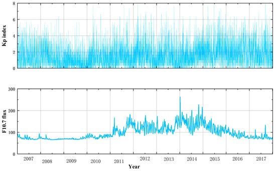
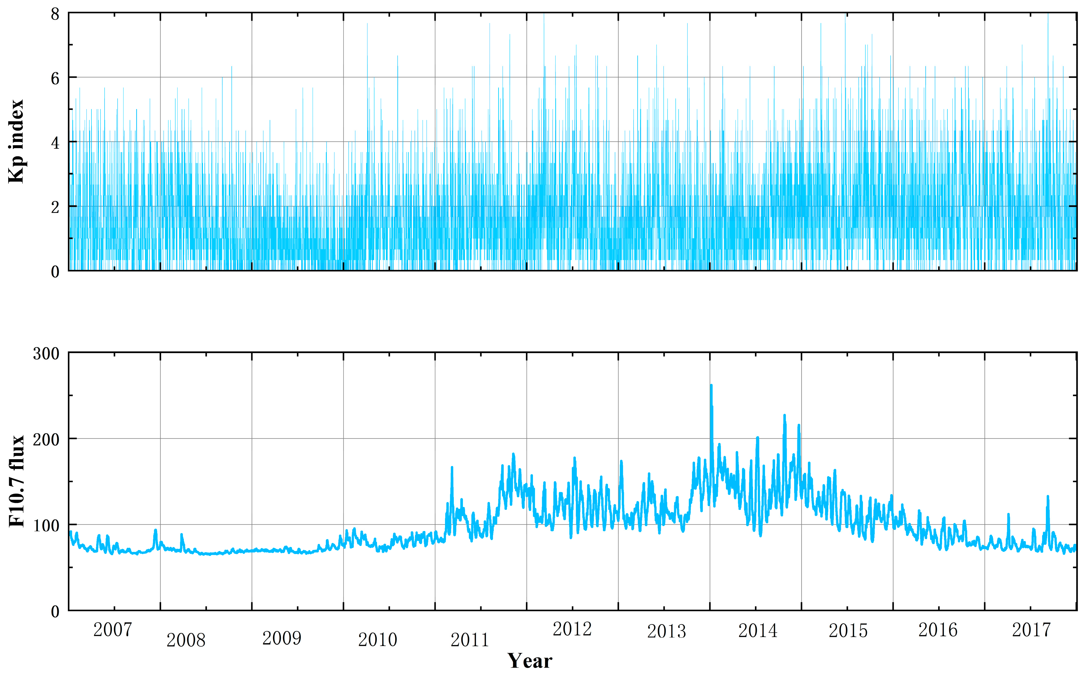
To characterize the background space weather conditions that may influence Es layer variability, two widely used indices describing solar and geomagnetic activity are employed in this study: the daily mean Kp index and the solar radio flux index F10.7. Both indices are used over the period from 2007 to 2017, consistent with the availability of the ionosonde observations analyzed in this work. The temporal variations in these indices during the study period are shown in Figure 1.
Figure 1.
Temporal variations in the daily mean Kp index (top panel) and the solar radio flux index F10.7 (bottom panel) during the study period. The Kp index represents global geomagnetic disturbance levels, while F10.7 serves as a proxy for solar extreme ultraviolet radiation.
2.3. Statistical Distribution of foEs Observations
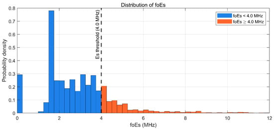
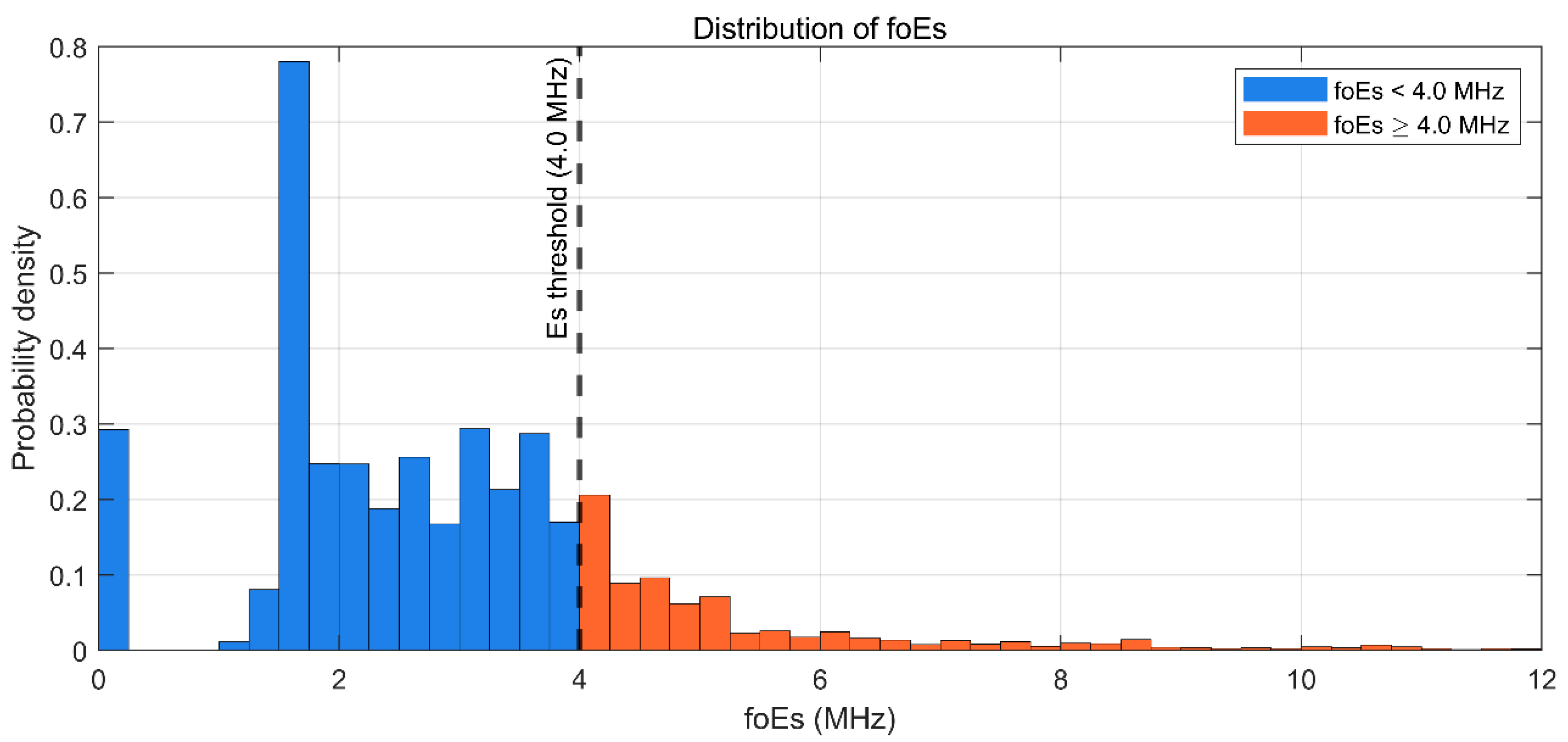
The foEs values collected from all stations exhibit a strongly skewed distribution in Figure 2. Most observations are concentrated at relatively low foEs levels, while events with large foEs values occur much less frequently and form a pronounced long-tailed distribution. In this study, we focus specifically on strong sporadic E (Es) events, which are characterized by substantially enhanced electron density and are known to exert a more pronounced influence on radio wave propagation [24]. Accordingly, a threshold of foEs = 4.0 MHz is adopted to distinguish strong Es events from weaker Es conditions. This threshold is not intended to imply that Es layers with foEs below 4.0 MHz are absent or unimportant in a physical sense; rather, it serves as a practical criterion to exclude background and weak Es conditions whose impact on radio propagation is generally limited.
Figure 2.
Probability density distribution of foEs values aggregated across all observation stations. The dashed vertical line denotes the threshold foEs = 4.0 MHz adopted to separate strong Es events from weak Es and background ionospheric conditions.
3. Method
In this study, a two-stage neural network framework is developed to predict the intensity of ionospheric Es layers. The proposed framework is motivated by the pronounced intermittency of Es occurrence and the severe imbalance between Es and non-Es samples, which often lead to systematic underestimation of strong Es events in conventional single-stage regression models. Observational statistics show that foEs exhibits a highly skewed distribution with a clear separation between background conditions and Es events, and a threshold of strong foEs = 4.0 MHz is therefore adopted to identify Es occurrence. To address this issue, the Es prediction task is decomposed into two successive and complementary processes: strong Es occurrence identification and Es intensity estimation conditioned on occurrence.
3.1. Model Framework
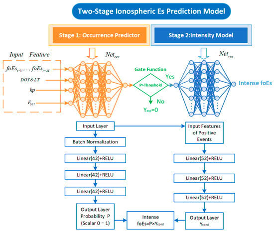
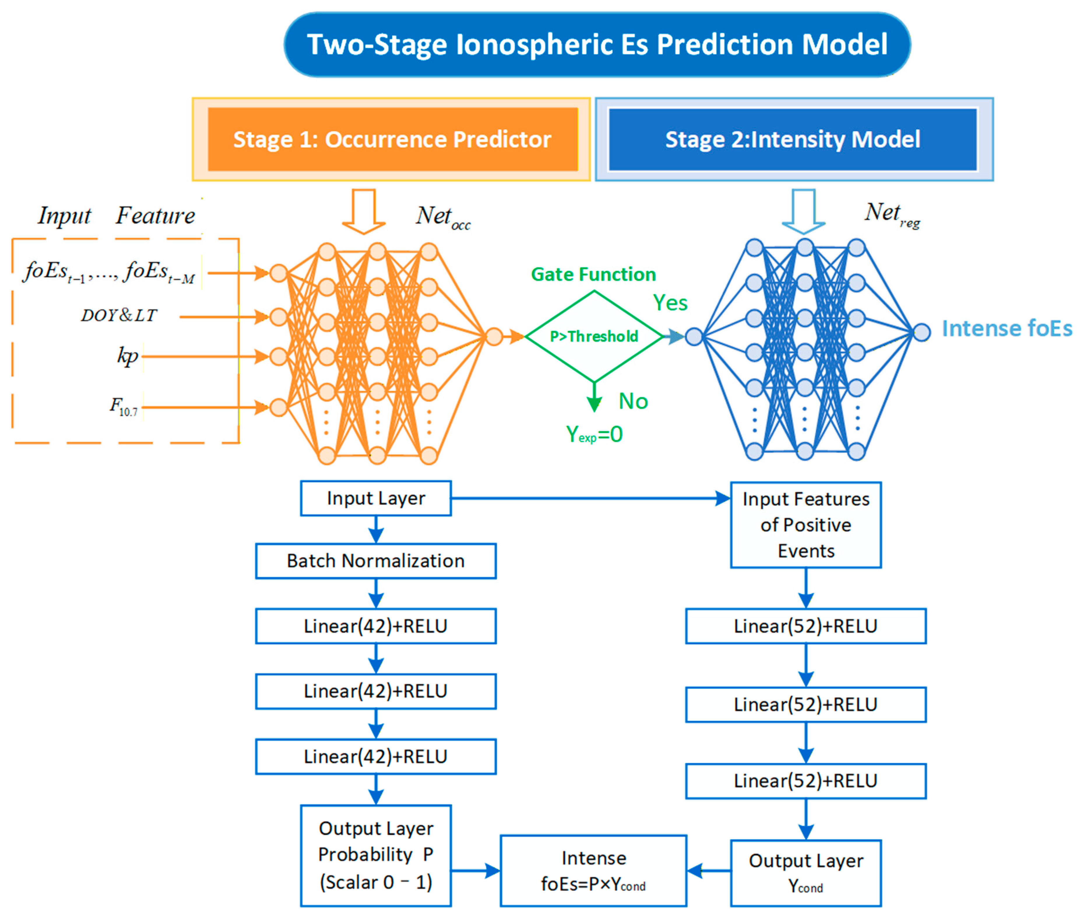
Figure 3 illustrates the architecture of the proposed two-stage ionospheric Es prediction model. The first stage aims to estimate the probability of Es occurrence across all input conditions based on various temporal and geophysical features. The occurrence prediction network, denoted as netocc, employs a fully connected deep learning architecture. It consists of an input layer, a Batch Normalization layer to stabilize and accelerate training, and three hidden linear layers, each containing 42 neurons and integrated with ReLU activation functions. The final layer utilizes a Sigmoid function to output a continuous probability value P in [0, 1], representing the likelihood of an Es event.
Figure 3.
Detailed architecture of the proposed two-stage prediction model. The framework includes Stage 1 netocc for occurrence probability P and Stage 2 netreg for conditional intensity Ycond. Both stages utilize fully connected architectures with Batch Normalization and three hidden linear layers (with 42 and 52 units respectively) followed by ReLU activations. A gating mechanism routes event-only samples to Stage 2 based on a threshold. The final output is calculated as Yexp = P × Ycond.
The input features of netocc include historical foEs information, temporal descriptors (day of year and local time), and space weather indices such as the kp index and the F10.7 solar flux. The use of local time, rather than universal time (UT), is physically motivated and consistent with recent findings emphasizing the LT dependence of sporadic E formation and diurnal variability inferred from ionosonde observations [25]. These features jointly characterize the seasonal variability, diurnal modulation, and solar–geomagnetic forcing associated with Es formation.
To explicitly distinguish Es events from non-events, a gating strategy is applied to the probabilistic output. Samples with predicted probabilities exceeding a predefined threshold are identified as Es events and passed to the second stage. This mechanism effectively mitigates the “dilution effect” caused by the overwhelming number of non-Es samples, allowing the subsequent regression model to focus on physically significant events.
The second stage performs Es intensity estimation conditioned on the occurrence identified in the first stage. The conditional intensity regression network, netreg, is trained exclusively on the Es-event samples. Following a similar structure to the first stage, netreg incorporates Batch Normalization and three hidden linear layers (52 neurons each) with ReLU activations. It outputs the conditional intensity Ycond, which corresponds to the predicted intense foEs given that an event has occurred.
By restricting the regression task to event-only samples, the conditional regression network avoids the dilution effect caused by the overwhelming number of non-Es cases and enhances the model’s capability to capture the amplitude variability and peak characteristics of Es events.
To produce a continuous full-field prediction, the final expected Es intensity Yexp is calculated as
where P is the occurrence probability and Ycond is the conditional intensity. This formulation preserves the probabilistic nature of the prediction while ensuring physically meaningful intensity estimates.
Both neural networks are implemented using fully connected architectures and are trained independently. The occurrence model is optimized using a classification loss function, whereas the intensity model is trained using a regression loss function evaluated only on Es-event samples. The dataset is randomly shuffled and divided into training, validation, and test subsets to ensure robust evaluation. Model performance is assessed using both qualitative comparisons of spatiotemporal distributions and quantitative event-only metrics, including mean absolute error (MAE), root mean square error (RMSE), and mean relative error (MRE). By explicitly separating Es detection from intensity estimation, the proposed two-stage framework improves sensitivity to strong Es events and enhances the robustness of Es intensity prediction across different stations and geophysical conditions.
3.2. Model Training Performance
In this study, ionosonde observations from a total of eleven stations are analyzed. For the Southern Hemisphere stations, data spanning the period 2007–2014 are employed. The datasets from 2007 and 2009–2013 are assigned to the training set, data from 2014 are used for validation, and observations from 2008 are reserved as an independent test set. For the Northern Hemisphere stations, ionosonde data covering 2011–2017 are utilized. Observations from 2011 to 2014 and 2016 constitute the training set, data from 2017 are used for validation, and data from 2015 are designated as the test set. This year-based temporal partitioning ensures strict independence between the training, validation, and test datasets, thereby enabling a robust assessment of the model’s generalization performance under different solar and geomagnetic conditions.
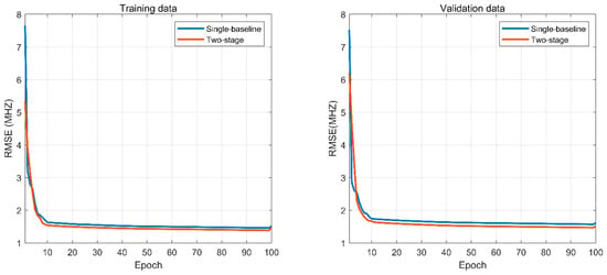
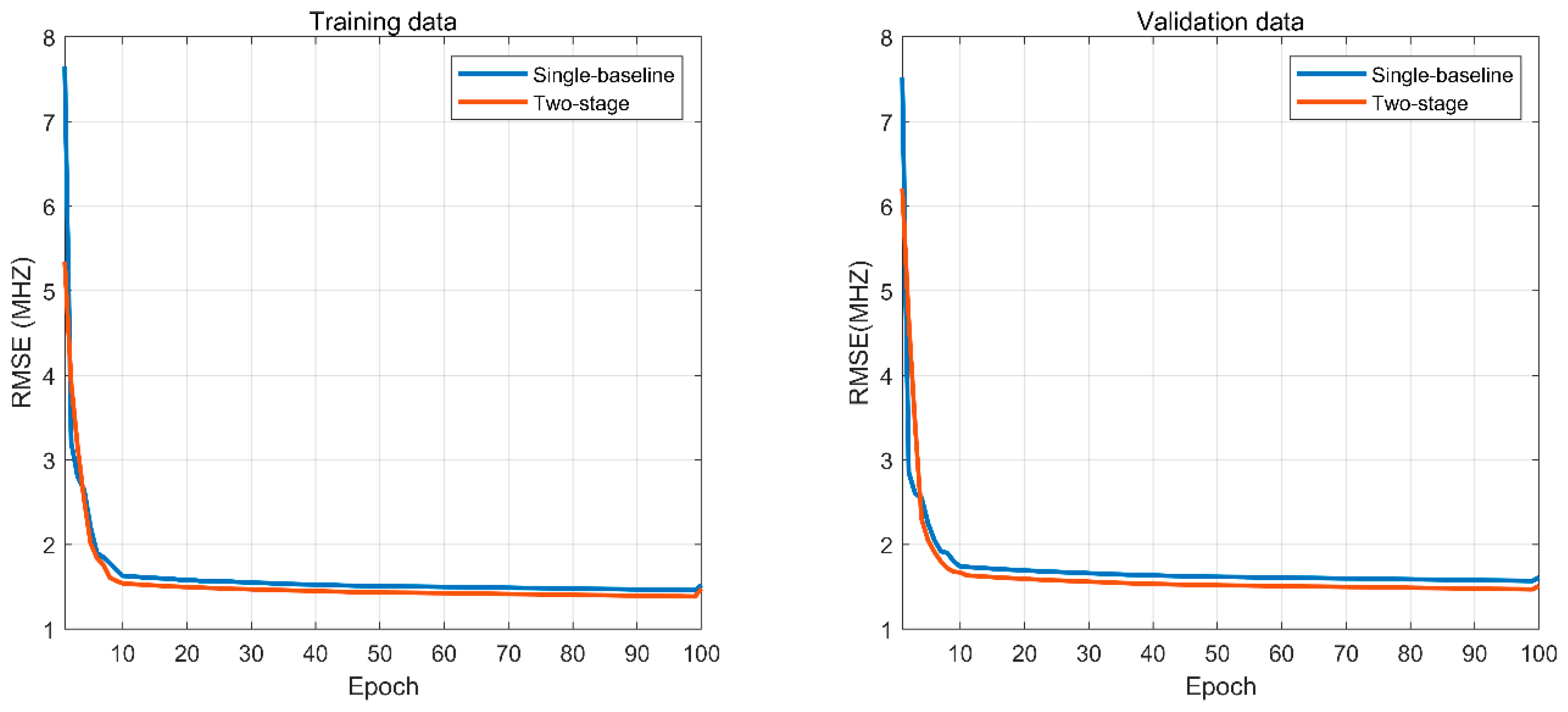
Figure 4 shows the variation in RMSE with training epochs for the single-baseline model and the two-stage model on the training set (left) and the validation set (right). For both models, the RMSE decreases rapidly during the early training stage. For example, on the training set, the RMSE drops from approximately 7.6 MHz (single-baseline) and 5.3 MHz (two-stage) to about 1.6 MHz within the first 10 epochs, after which the decrease becomes gradual and the models converge steadily. Compared with the single-baseline model, the two-stage model converges faster and achieves lower final RMSE values on both the training and validation sets of approximately 1.52 MHz, indicating improved prediction accuracy and generalization performance.
Figure 4.
The RMSEs of the single-baseline model and the two-stage model for the training set (left) and the validation set (right) with the number of epochs. The blue line represents the single-baseline model, and the orange line represents the two-stage model.
4. Results
The performance of the proposed two-stage framework is evaluated using a combination of qualitative and quantitative analyses. The evaluation focuses on the model’s ability to represent Es occurrence, predict conditional Es intensity, and produce full-field expected intensity estimates. Model performance is examined through spatiotemporal distribution maps and event-only statistical metrics across multiple stations and forecast lead times.
4.1. Performance of Strong Es Occurrence Prediction
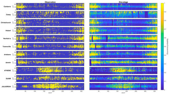
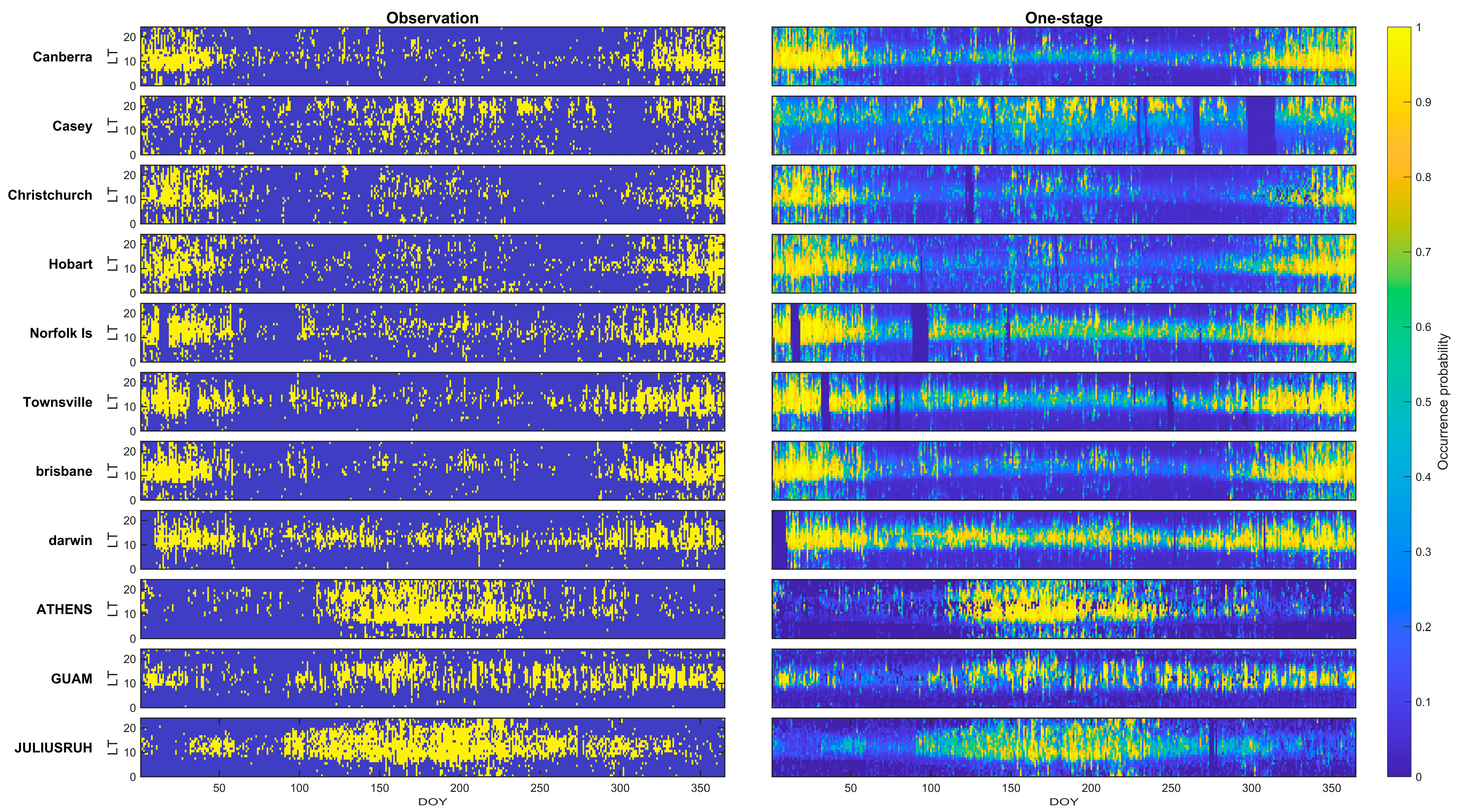
Figure 5 presents a comparison between the observed Es occurrence and the model-predicted Es occurrence probability for all stations in the Day of Year–Local Time (DOY–LT) domain. The left column shows the observed Es occurrence, where Es events are sparsely distributed in time and local time, highlighting the highly intermittent nature of Es. The right column displays the corresponding occurrence probability predicted by the first-stage occurrence network.
Figure 5.
DOY versus LT distributions of observed Es occurrence (left panels) and predicted Es occurrence probability from the first-stage model (right panels) for eight ionosonde stations. Each row corresponds to one station. The predicted probability fields reproduce the main seasonal and diurnal characteristics of Es occurrence and show good agreement with observed occurrence patterns.
Overall, the model successfully captures the large-scale seasonal and diurnal patterns of Es occurrence at most stations, as reflected by the enhanced probabilities during known favorable periods. In contrast to the binary and highly fragmented observation maps, the predicted probability fields exhibit smoother and more continuous structures, indicating that the model learns the underlying climatological tendency of Es occurrence rather than individual isolated events. Discrepancies are evident at some stations, where localized or short-lived observed events are not always associated with pronounced probability enhancements, leading to occasional missed detections. Conversely, the model sometimes produces elevated probabilities during periods with weak or no observed Es activity, suggesting false alarms. These differences reflect the intrinsic difficulty of predicting high-Es events and partly arise from the probabilistic nature of the occurrence modeling.
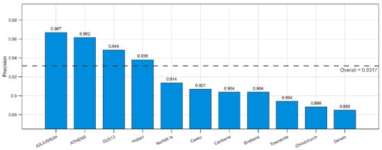
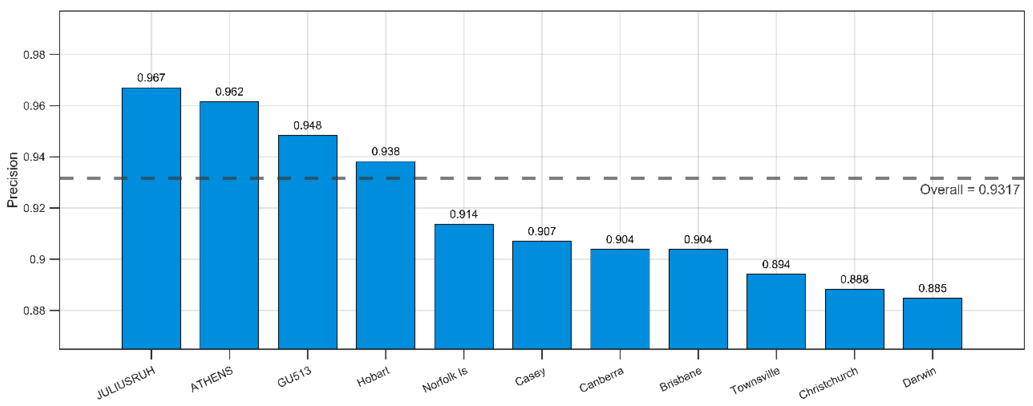
Figure 6 presents a comparison of one-station precision for Es occurrence prediction across different ionosonde stations, providing an assessment of the station-dependent reliability of the model. The horizontal axis lists the stations (from JULIUSRUH to Darwin), while the vertical axis denotes the precision. Each blue bar represents the precision achieved at an individual station, with the exact value annotated on top of the bar, ranging approximately from 0.885 to 0.967. The gray dashed horizontal line indicates the overall mean precision across all stations, which is 0.9317, and serves as a reference level for evaluating individual station performance. Stations such as JULIUSRUH, AT138, and GU513 exhibit precision values well above the overall average, indicating particularly strong predictive reliability, whereas Townsville, Christchurch, and Darwin fall below the mean, with Darwin showing the lowest precision. Overall, the results demonstrate that the model achieves consistently high precision across most stations, while also revealing clear inter-station variability in predictive performance.
Figure 6.
One-station precision of Es occurrence prediction at 11 ionosonde stations. Blue bars show the precision for each station, and the dashed line indicates the overall mean precision.
4.2. Performance of Strong Es Intensity Prediction
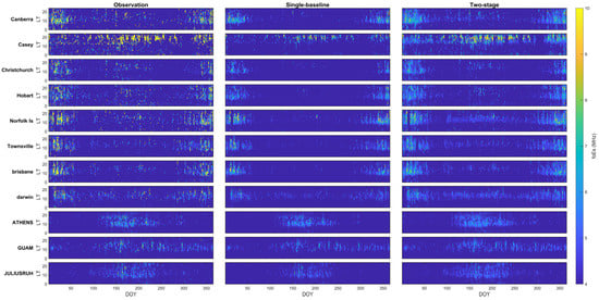
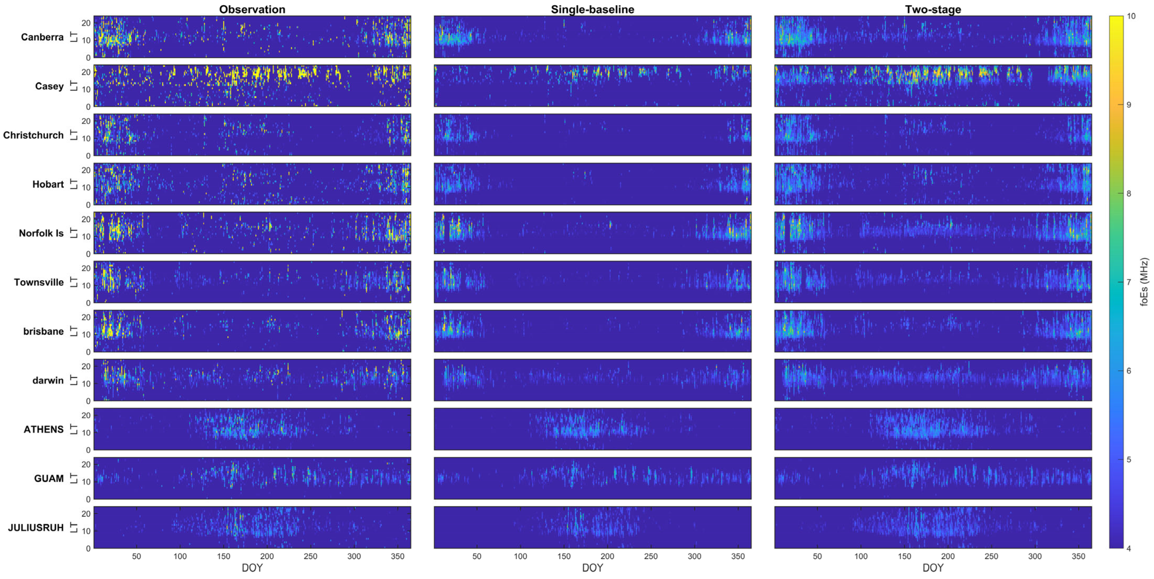
To visually assess the capability of the proposed two-stage framework in reproducing the spatiotemporal characteristics of Es intensity, Figure 7 presents a comparison between ionosonde-observed foEs distributions and model predictions of DOY–LT coordinates for multiple stations. For each station, the left panels show the observed foEs values, while the right panels display the corresponding predictions from the proposed two-stage framework. This qualitative comparison demonstrates that the two-stage model effectively captures the dominant seasonal and diurnal patterns of Es intensity and suppresses spurious high-intensity values under non-Es conditions.
Figure 7.
Comparison of observed (left panels) and model-predicted (right panels) foEs distributions in DOY–LT coordinates for eight ionosonde stations. The model results are obtained from the two-stage framework by combining occurrence probability and conditional intensity predictions. The color scale represents foEs values in MHZ.
It is evident that the single-stage baseline model exhibits a pronounced smoothing effect, largely underestimating the peak intensities of strong Es events and failing to capture the sharp intermittency of the layers. Conversely, the qualitative comparison demonstrates that the two-stage model effectively captures the dominant seasonal and diurnal patterns of Es intensity while preserving the discrete high-intensity structures. By suppressing spurious values under non-Es conditions and recovering extreme values during Es events, the two-stage framework yields a spatiotemporal distribution that is significantly closer to the observational ground truth than the baseline model.
To quantitatively evaluate the improvement introduced by the two-stage design, Table 2 summarizes the performance metrics (MAE, MRE, and RMSE) of the proposed framework in comparison with a conventional single-stage baseline model. For all stations, the two-stage framework consistently outperforms the baseline model, achieving reduced errors across all three metrics. The improvement is particularly pronounced at stations characterized by stronger Es intermittency, where the baseline model tends to overestimate background conditions or underestimate strong Es events.
Table 2.
Performance metrics of foEs prediction at 8 stations.
For most mid- and low-latitude stations, the two-stage model significantly reduces MAE and RMSE relative to the baseline, indicating that explicitly separating Es occurrence detection from conditional intensity regression effectively mitigates the impact of severe sample imbalance and enhances sensitivity to strong Es events. The aggregated results across all stations further confirm this improvement, with overall RMSE decreasing from 2.311 MHz for the baseline model to 1.897 MHz for the two-stage framework.
Despite the overall performance enhancement, degraded prediction accuracy persists at a limited number of stations, most notably at Casey. As a high-latitude station, Casey is subject to more complex and rapidly varying ionospheric conditions, including enhanced geomagnetic activity, auroral forcing, and dynamic electrodynamic processes. These factors increase background variability and the occurrence of short-lived extreme Es events, posing inherent challenges for data-driven prediction models. Consequently, the larger errors at Casey reflect both model limitations and the intrinsic difficulty of forecasting Es intensity in high-latitude environments.
4.3. Seasonal and Local Time Variability of RMSE
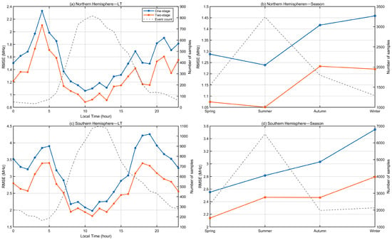
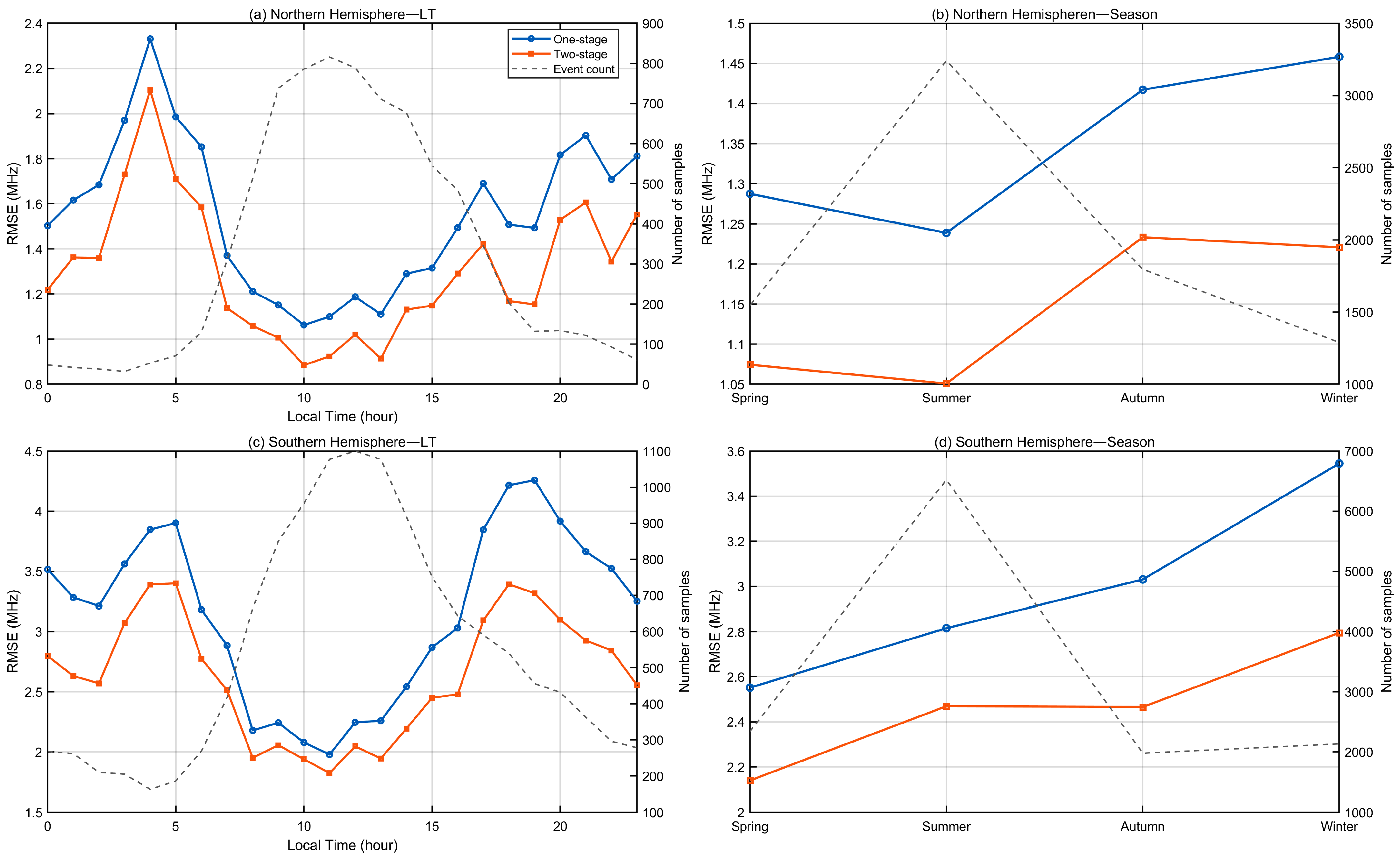
Figure 8 shows the variation in foEs prediction RMSE with local time and season in the Northern and Southern Hemispheres, comparing the performance of the one-stage and two-stage models. In the Northern Hemisphere, the one-stage model exhibits pronounced RMSE peaks during the early morning hours (approximately 03–06 LT), whereas the two-stage model maintains lower errors throughout the entire diurnal cycle, with particularly notable improvements during daytime and evening hours. In the Southern Hemisphere, overall RMSE levels are higher, indicating stronger background variability; nevertheless, the two-stage model consistently outperforms the one-stage model across all local times, with the largest error reductions occurring during nighttime and evening periods. On the seasonal scale, RMSE in the Northern Hemisphere reaches a minimum in summer, coinciding with the largest number of Es-event samples, and increases markedly in autumn and winter, while in the Southern Hemisphere, RMSE shows a gradual increase from spring to winter. Overall, the two-stage model systematically reduces prediction errors under different local time and seasonal conditions, with its advantages being most pronounced during periods characterized by limited Es-event samples, demonstrating its effectiveness in mitigating the impact of sample imbalance on Es intensity prediction.
Figure 8.
Variation in foEs prediction RMSE with local time and season in the Northern and Southern Hemispheres. Panels (a,c) show RMSE variation with local time, and panels (b,d) show RMSE variation with season. The one-stage and two-stage model results are compared, and the gray dashed lines indicate the number of Es-event samples in each bin.
5. Conclusions
This study developed a unified two-stage neural network framework for forecasting Es occurrence and intensity using multi-station ionosonde foEs observations and space weather drivers. By decomposing the prediction problem into (i) probabilistic Es occurrence modeling and (ii) intensity regression conditioned on Es presence, the framework explicitly addresses the strong intermittency of Es and the severe imbalance between Es and non-Es samples. The occurrence network produces smooth and physically interpretable probability fields that capture the dominant seasonal and local time tendencies of Es activity across stations. The conditional intensity network focuses on Es-present conditions and provides intensity estimates that better represent the variability of foEs when events occur. Combining the occurrence probability with the conditional intensity yields a continuous expected-intensity prediction, which suppresses spurious high-intensity outputs under non-Es conditions while retaining event-related enhancements. Overall, the proposed framework offers a practical strategy for probabilistic and conditional prediction of Es layers within a single model across multiple stations.
Several limitations should be addressed in future work. First, prediction skill in high-latitude environments remains comparatively degraded, suggesting that additional drivers related to auroral forcing and electrodynamic variability are needed. Second, the coupling between occurrence and intensity can be further improved through calibration of occurrence probabilities and event-oriented training strategies that emphasize strong Es episodes. Finally, extending the framework to incorporate additional observation modalities (e.g., GNSS radio occultation-based proxies) and to quantify uncertainty would further enhance robustness and applicability for operational communication and navigation support.
Author Contributions
Author Contributions: Conceptualization, L.L. and D.Y.; methodology, L.L.; software, L.L.; validation, L.L.; formal analysis, L.L.; investigation, L.L.; resources, D.Y.; data curation, L.L.; writing—original draft preparation, L.L.; writing—review and editing, D.Y.; visualization, L.L.; supervision, D.Y.; project administration, D.Y.; funding acquisition, D.Y. All authors have read and agreed to the published version of the manuscript.
Funding
This research was funded by the National Natural Science Foundation of China, grant number 42404179, and the Fundamental Research Funds for the Provincial Universities of Zhejiang, grant number GK24990929001-034.
Data Availability Statement
The Australian Bureau of Meteorology—Space Weather Services (SWS, http://www.sws.bom.gov.au/World_Data_Centre, accessed on 12 January 2026) website was used to obtain altimeter data. The Kp index was obtained from NASA’s OMNIWeb portal (https://omniweb.gsfc.nasa.gov/form/dx1.html, accessed on 12 January 2026), and the F10.7 solar flux data were retrieved from NOAA’s Space Weather Prediction Center (https://www.swpc.noaa.gov/products/solar-geophysical-data, accessed on 12 January 2026). To ensure reproducibility, the model was implemented in MATLAB R2024a (MathWorks, Natick, MA, USA). The core model architecture, representative data samples, and the scripts used to generate the figures and tables in this study have been uploaded to GitHub and are publicly available at: https://github.com/liuliccc/A-Two-Stage-Machine-Learning-Framework-for-Predicting-Sporadic-E-Occurrence-and-Intensity (accessed on 12 January 2026).
Acknowledgments
The authors gratefully acknowledge the altimeter data provided by the Australian Bureau of Meteorology—Space Weather Services (SWS) website.
Conflicts of Interest
The authors declare no conflict of interest.
References
- Zeng, Z.; Sokolovskiy, S. Effect of sporadic E clouds on GPS radio occultation signals. Geophys. Res. Lett. 2010, 37, L18817. [Google Scholar] [CrossRef] [Scilit]
- Andoh, S.; Saito, A.; Shinagawa, H.; Ejiri, M.K. First simulations of day-to-day variability of mid-latitude sporadic E layer structures. Earth Planets Space 2020, 72, 165. [Google Scholar] [CrossRef] [Scilit]
- Haldoupis, C. A tutorial review on sporadic E layers. In Aeronomy of the Earth’s Atmosphere and Ionosphere; Springer: Dordrecht, The Netherlands, 2011; pp. 381–394. [Google Scholar]
- Kunduri, B.S.R.; Erickson, P.J.; Baker, J.B.; Ruohoniemi, J.M.; Galkin, I.; Sterne, K. Dynamics of mid-latitude sporadic-E and its impact on HF propagation in the North American sector. J. Geophys. Res. Space Phys. 2023, 128, e2023JA031455. [Google Scholar] [CrossRef] [Scilit]
- Saito, S.; Hosokawa, K.; Sakai, J.; Tomizawa, I. Study of structures of the sporadic E layer by using dense GNSS network observations. NAVIGATION J. Inst. Navig. 2021, 68, 751–758. [Google Scholar] [CrossRef] [Scilit]
- Moro, J.; Resende, L.; Denardini, C.; Xu, J.; Batista, I.; Andrioli, V.; Carrasco, A.; Batista, P.; Schuch, N. Equatorial E region electric fields and sporadic E layer responses to the recovery phase of the November 2004 geomagnetic storm. J. Geophys. Res. Space Phys. 2017, 122, 12517–12533. [Google Scholar] [CrossRef] [Scilit]
- Da Silva, L.A.; Shi, J.; Vieira, L.E.; Agapitov, O.V.; Resende, L.C.A.; Alves, L.R.; Sibeck, D.; Deggeroni, V.; Marchezi, J.P.; Chen, S. Why can the auroral-type sporadic E layer be detected over the South America Magnetic Anomaly (SAMA) region? An investigation of a case study under the influence of the high-speed solar wind stream. Front. Astron. Space Sci. 2023, 10, 1197430. [Google Scholar] [CrossRef] [Scilit]
- Niu, J.; Fang, H.-x. An empirical model of the sporadic E layer intensity based on COSMIC radio occultation observations. Space Weather 2023, 21, e2022SW003280. [Google Scholar] [CrossRef] [Scilit]
- Hodos, T.J.; Nava, O.A.; Dao, E.V.; Emmons, D.J. Global sporadic-E occurrence rate climatology using GPS radio occultation and ionosonde data. J. Geophys. Res. Space Phys. 2022, 127, e2022JA030795. [Google Scholar] [CrossRef] [Scilit]
- Gooch, J.Y.; Colman, J.J.; Nava, O.A.; Emmons, D.J. Global ionosonde and GPS radio occultation sporadic-E intensity and height comparison. J. Atmos. Sol.-Terr. Phys. 2020, 199, 105200. [Google Scholar] [CrossRef] [Scilit]
- Niu, J.; Fang, H.; Wang, X.-x.; Weng, L.; Guo, L. Analysis of the ionosphere irregularities in E region based on COSMIC occultation data. Adv. Space Res. 2015, 56, 1895–1900. [Google Scholar] [CrossRef] [Scilit]
- Niu, J.; Weng, L.; Meng, X.; Fang, H. Morphology of ionospheric sporadic E layer intensity based on COSMIC occultation data in the midlatitude and low-latitude regions. J. Geophys. Res. Space Phys. 2019, 124, 4796–4808. [Google Scholar] [CrossRef] [Scilit]
- Yu, B.; Xue, X.; Scott, C.J.; Yue, X.; Dou, X. An empirical model of the ionospheric sporadic E layer based on GNSS radio occultation data. Space Weather 2022, 20, e2022SW003113. [Google Scholar] [CrossRef] [Scilit]
- Tang, L.; Li, J.; Zhang, F.; Zou, F. Comparative study of ionospheric sporadic E occurrence rates using SNRnstd and S4 derived from GPS radio occultation. GPS Solut. 2023, 27, 120. [Google Scholar] [CrossRef] [Scilit]
- Resende, L.C.; Arras, C.; Batista, I.S.; Denardini, C.M.; Bertollotto, T.O.; Moro, J. Study of sporadic E layers based on GPS radio occultation measurements and digisonde data over the Brazilian region. Ann. Geophys. 2018, 36, 587–593. [Google Scholar] [CrossRef] [Scilit]
- Abadi, P.; Saito, S.; Srigutomo, W. Low-latitude scintillation occurrences around the equatorial anomaly crest over Indonesia. Ann. Geophys. 2014, 32, 7–17. [Google Scholar] [CrossRef] [Scilit]
- Romero, R.; Dovis, F. Effect of interference in the calculation of the amplitude scintillation index S4. In Proceedings of the 2013 International Conference on Localization and GNSS (ICL-GNSS), Turin, Italy, 25–27 June 2013; pp. 1–6. [Google Scholar]
- Arras, C. A Global Survey of Sporadic E Layers Based on GPS Radio Occultations by CHAMP, GRACE and FORMOSAT–3/COSMIC; Deutsches GeoForschungsZentrum GFZ Potsdam: Potsdam, Germany, 2010. [Google Scholar]
- Yue, X.; Schreiner, W.; Zeng, Z.; Kuo, Y.-H.; Xue, X. Case study on complex sporadic E layers observed by GPS radio occultations. Atmos. Meas. Tech. 2015, 8, 225–236. [Google Scholar] [CrossRef] [Scilit]
- Arras, C.; Wickert, J. Estimation of ionospheric sporadic E intensities from GPS radio occultation measurements. J. Atmos. Sol.-Terr. Phys. 2018, 171, 60–63. [Google Scholar] [CrossRef] [Scilit]
- Carmona, R.A.; Nava, O.A.; Dao, E.V.; Emmons, D.J. A comparison of sporadic-E occurrence rates using GPS radio occultation and ionosonde measurements. Remote. Sens. 2022, 14, 581. [Google Scholar] [CrossRef] [Scilit]
- Yang, D.; Fang, H. A low-latitude three-dimensional ionospheric electron density model based on radio occultation data using artificial neural networks with prior knowledge. Space Weather 2023, 21, e2022SW003299. [Google Scholar] [CrossRef] [Scilit]
- Liu, L.; Zou, S.; Yao, Y.; Wang, Z. Forecasting global ionospheric TEC using deep learning approach. Space Weather 2020, 18, e2020SW002501. [Google Scholar] [CrossRef] [Scilit]
- Cameron, T.; Fiori, R.; Themens, D.; Warrington, E.; Thayaparan, T.; Galeschuk, D. Evaluation of the effect of sporadic-E on high frequency radio wave propagation in the Arctic. J. Atmos. Sol.-Terr. Phys. 2022, 228, 105826. [Google Scholar] [CrossRef] [Scilit]
- Haldoupis, C.; Haralambous, H.; Meek, C.; Mathews, J.D. Understanding the diurnal cycle of midlatitude sporadic E. The role of metal atoms. J. Geophys. Res. Space Phys. 2023, 128, e2023JA031336. [Google Scholar] [CrossRef] [Scilit]

Disclaimer/Publisher’s Note: The statements, opinions and data contained in all publications are solely those of the individual author(s) and contributor(s) and not of MDPI and/or the editor(s). MDPI and/or the editor(s) disclaim responsibility for any injury to people or property resulting from any ideas, methods, instructions or products referred to in the content. |
© 2026 by the authors. Licensee MDPI, Basel, Switzerland. This article is an open access article distributed under the terms and conditions of the Creative Commons Attribution (CC BY) license.