Conformal Holographic Dark Energy and the Neutrino-Mass Tension

Abstract

Recent DESI results suggest a preference for evolving dark energy (DE) over a cosmological constant, motivating the exploration of alternative models for the background expansion. These data also lead to neutrino-mass constraints close to the lower bounds permitted by oscillation experiments. In this work, we propose and test a conformal holographic dark energy (CHDE) model in which the DE density depends on a power law of the conformal time, characterized by an exponent n. The model introduces one additional parameter relative to ΛCDM and reduces to it in the limit $n=0$. We confront CHDE with BAO, CMB, and SNe Ia datasets, following the combinations used by DESI, and perform parameter inference in both flat and non-flat cosmologies. We find a consistent preference for $n\simeq -0.25$ to $-0.32$, with uncertainties below $\pm 0.1$, and disfavor the ΛCDM limit at the $4.4$–$4.5\sigma$ level; however, the model-comparison statistics provide no consistent preference for CHDE over ΛCDM. The resulting neutrino-mass constraints remain compatible with terrestrial limits and yield posterior distributions that peak at positive values, avoiding the negative-mass preference found in ΛCDM. The CHDE model is therefore consistent with current observational constraints and provides a viable alternative to constant dark energy.

1. Introduction

The standard model of cosmology is based on a content of baryons, photons, neutrinos, cold dark matter, and dark energy (DE). Although we do not know the origin of cold dark matter, we have characterized its gravitational effects at different astrophysical and cosmological scales [1], which seem consistent with its cold origin, but interesting alternatives have been discussed in the literature, such as warm and fuzzy dark matter [2,3]. On the other hand, we know less about DE, but it is clear that a cosmological constant is the simplest way to account for the cosmic acceleration. For many years, the cosmological constant plus cold dark matter (ΛCDM) model has been remarkably successful in explaining a wide range of cosmological observations, including Type Ia supernova (SNe Ia) distance measurements, cosmic chronometers, the Cosmic Microwave Background (CMB), and large-scale structure clustering statistics. However, the cosmological constant has recently been called into question by the joint analysis of Baryon Acoustic Oscillations (BAO) performed by the Dark Energy Spectroscopic Instrument (DESI) collaboration Year 1 [4,5,6] and Year 2 [7,8], DES final BAO [9], and supernova results: Pantheon+ [10,11], Union3 [12], and the Dark Energy Survey (DES) Year 5 [13]. Their analysis suggests that the DE responsible for the current epoch of cosmic acceleration is decreasing at present. In any case, the results provide evidence in favor of a dynamical form of dark energy rather than a strictly constant one. Because the origin of this behavior remains unclear, numerous alternative explanations have been proposed. These can be broadly classified into fundamental theoretical models and parameterized phenomenological models.

As far as we know, cosmological data does not reveal DE clustering properties, but it mainly manifests its effect in the background dynamics (apart from the integrated Sachs–Wolfe (ISW) effect). Therefore, when thinking of passing from a cosmological constant to a function, it seems appealing to associate a cosmological function with no clustering properties, or, if any, at very large distances such as horizon scales, and that is why a holographic Universe is accommodated in a natural way. Holographic dark energy (HDE) has been a popular model for years, and  different realizations of it have been put forward [14,15,16]. Here, we discuss a holographic model that depends on the conformal time. However, our model is different from the well-known agegraphic models [15,17], in which matter conservation is defined apart from the Einstein equations, which are assumed to be valid. In our case, the cosmological DE function will be explicitly written in the Einstein equations, so energy conservation demands an interaction between our HDE model and dark matter in particular. Our model has the mathematical properties of a vacuum DE model, such as the one presented in refs. [18,19].

On the other hand, recent cosmological measurements of the neutrino mass by the DESI collaboration [7] suggest extremely small values that may conflict with limits established by terrestrial neutrino oscillation experiments; see also [20]. Some DESI data combinations even seem to disfavor both the normal and inverted mass hierarchies, and the preferred values in the statistical analyses tend to lie in nonphysical, negative regions [21]. These tensions motivate the exploration of alternative cosmological scenarios. One proposal is to allow spatial curvature to vary, which weakens the constraints and shifts the inferred values toward more physically plausible ones [22]. However, even in this case, the most likely value remains close to zero, indicating that a full resolution of the issue may require analyses in which effectively negative neutrino masses are allowed. Indeed, this latter analysis suggests that curvature alone does not provide a solution to the tension [23]. In this context, DE models should be examined to assess whether they can resolve, or at least alleviate, the tension in the inferred neutrino mass. For  instance, the $w_0{w}_a$ CDM model [23,24,25] provides partial relief, although it does not fully eliminate the problem once all datasets are included. Other DE models appear to resolve the issue for particular choices of the equation of state that cross the phantom divide ($w=-1$) [26], whereas our model keeps $w=-1$, with the time dependence entering through the interaction term. In this work, we investigate this question within the framework of our proposed model.

The aim of this paper is to develop and observationally test a conformal holographic dark energy (CHDE) model as an alternative to ΛCDM, and to assess whether it can alleviate the tension between cosmological neutrino-mass constraints and the lower bounds inferred from terrestrial oscillation experiments. In this model, the  dark energy density follows a power law in conformal time and exchanges energy with dark matter while retaining an equation of state $w=-1$. We implement the model in the Cosmic Linear Anisotropy Solving System (class) and perform Bayesian parameter inference using Markov chain Monte Carlo (MCMC) sampling with Cobaya, employing combinations of DESI Data Release 2 (DR2) BAO, Planck CMB, Atacama Cosmology Telescope (ACT) lensing, and Type Ia supernova data. We consider both spatially flat and non-flat cosmologies to constrain the model parameters, examine the inferred sum of neutrino masses, and  compare the model’s statistical performance with that of ΛCDM.

This work is organized as follows: In Section 2, we present the CHDE model and derive the relevant equations. In Section 3, we employ different datasets and free parameters to extract the physical information of the model. Finally, in Section 4, we review our results and conclude. One appendix is provided that presents our theoretical implementation in class.

2. The CHDE Model

We start with the Einstein equations with a holographic term given by the following [27]:

$$R^{\mu \nu }-{\displaystyle \frac{1}{2}}R{g}^{\mu \nu }+\mathcal{M}{g}^{\mu \nu }={\kappa }^2{T}^{\mu \nu },$$

(1)

where ${\kappa }^2=8\pi G/c^4$; G is Newton’s gravitational constant, $T^{\mu \nu }$ contains the standard matter pieces of the standard cosmological model (baryons, cold dark matter (DM), and relativistic particles), and $\mathcal{M}$ is a holographic function that will depend on the horizon distance and will play the role of a cosmological dark energy function. One may postulate different holographic functions, see, e.g., [15], which typically depend on the physical horizon. But one can also consider the comoving horizon. In ref. [28], the authors opted for this option, taking $\mathcal{M}\sim {\displaystyle \frac{1}{{\lambda }^2}}$, where $\lambda$ is the cosmological length scale given by $\lambda ={\displaystyle \frac{c}{H_0}}{R}_H$, where $R_H=H_0{\int }_0^{t}d{t}^{\prime }/a\left(t^{\prime }\right)$ is the Friedmann–Robertson–Walker (FRW) comoving horizon, where $a\left(t\right)$ is the scale factor, t the cosmic time and $H_0$ the Hubble constant. This model was motivated by its connection to de Proca gravity and the interpretation that it represents a gravitational wave background [28]. The interpretation of the previous model in terms of a gravitational-wave background motivates exploring whether a dependence of the wave amplitude on the cosmological length scale $\lambda$ could modify the inverse-square scaling. Here, we adopt a phenomenological power-law generalization, rather than a first-principles derivation from that interpretation. Since $R_H=H_0\eta$, it is convenient to express the model in terms of conformal time, defined by $d\eta =dt/a\left(t\right)$. Our conformal holographic dark energy (CHDE) model is

$$\mathcal{M}=const.{\eta }^n,$$

(2)

where the exponent n is a constant and the $const$ is conveniently defined as $const=Q{H}_0^{n+2}$, with Q being a dimensionless constant of order one related to the cosmological function evaluated today, and $H_0^{-1}$ is of the order of the horizon at present that gives the proper units to $\mathcal{M}=Q{H}_0^2{\left(H_0\eta \right)}^n$, given that $H_0\eta$ is dimensionless. Equation (2) is a phenomenological ansatz motivated by the conformal-horizon dependence of the previously studied model. The power-law form provides a simple one-parameter extension of its inverse-square scaling: $n=-2$ recovers the previous model, whereas $n=0$ gives a constant dark energy density and recovers ΛCDM. Allowing n to vary therefore enables an observational test of departures from these two limits. The exponent n is constrained by cosmological observations, while Q is determined through the present-day closure relation, as described below.

Note that it is convenient to define ${\rho }_{\mathcal{M}}=\mathcal{M}/8\pi G$ and therefore

$${\mathrm{\Omega }}_{\mathcal{M}}={\displaystyle \frac{{\rho }_{\mathcal{M}}}{{\rho }_{c0}}}={\mathrm{\Omega }}_{\mathcal{M}}^{\left(0\right)}{\left({\displaystyle \frac{\eta }{{\eta }_0}}\right)}^n,$$

(3)

where ${\mathrm{\Omega }}_{\mathcal{M}}^{\left(0\right)}\equiv {\displaystyle \frac{1}{3}}Q{\left(H_0{\eta }_0\right)}^n$ and ${\rho }_{c0}$ is the standard critical density. Equation (3) is our cosmological function, in which the cosmological scale, ${\eta }_0\sim H_0^{-1}$, is the comoving scale evaluated at present times; in principle, it can be thought of as a fundamental scale responsible for DE. Assuming an FRW background geometry, the gravitational Equation (1) implies

$${\displaystyle \frac{{\mathcal{H}}^2}{H_0^2}}={\displaystyle \frac{{\mathrm{\Omega }}_b^{\left(0\right)}}{a}}+{\displaystyle \frac{{\mathrm{\Omega }}_{\gamma }^{\left(0\right)}}{a^2}}+{\mathrm{\Omega }}_k^{\left(0\right)}+{\mathrm{\Omega }}_{dm}^{\left(0\right)}{\displaystyle \frac{{\rho }_{dm}}{{\rho }_{dm}^{\left(0\right)}}}{a}^2+{\mathrm{\Omega }}_{\mathcal{M}}^{\left(0\right)}{a}^2{\left({\displaystyle \frac{\eta }{{\eta }_0}}\right)}^n,$$

(4)

where $\mathcal{H}\equiv {\displaystyle \frac{a^{\prime }}{a}}={\displaystyle \frac{1}{a}}{\displaystyle \frac{da}{d\eta }}$; we will also consider the curvature that can be added to this equation. For a fixed value of n, the CHDE model has the same number of free parameters as ΛCDM. In the fits presented here, however, n is varied freely, introducing one additional free parameter relative to ΛCDM. Note that one can recover the ΛCDM model for $n=0$; $n=-2$ was used in previous works by one of the authors [27,28]. On the other hand, if there is no interaction between DM and CHDE ($Q=0$), ${\rho }_{dm}\sim 1/a^3$, one recovers the Einstein de Sitter Universe (with no radiation and curvature). But, in general, matter conservation demands

$${\rho }_{dm}^{\prime }+3\mathcal{H}{\rho }_{dm}=-{\rho }_{\mathcal{M}}^{\prime }=-n{\displaystyle \frac{{\rho }_c^{\left(0\right)}}{{\eta }_0}}{\mathrm{\Omega }}_{\mathcal{M}}^{\left(0\right)}{\left({\displaystyle \frac{\eta }{{\eta }_0}}\right)}^{n-1}.$$

(5)

where ${\rho }_c^{\left(0\right)}\equiv 3H_0^2/8\pi G$. This equation specifies the interaction of DM with CHDE, in which one can directly observe that DM is created if $n<0$, and it is sourced by a time-decaying function for $n<1$. The CHDE is a geometric term, but in analogy to the ΛCDM model, it can be thought of as a perfect fluid, so that the r.h.s. of Equation (5) is equal to $-[{\rho }_{\mathcal{M}}^{\prime }+3\mathcal{H}(1+{\mathrm{w}}_{\mathcal{M}}){\rho }_{\mathcal{M}}]$; therefore, this equation shows that ${\mathrm{w}}_{\mathcal{M}}=-1$. This can also be seen from Equation (1): the relationship between ${\rho }_{\mathcal{M}}$ and $p_{\mathcal{M}}$ is given similar to the ΛCDM model, $T_{\mathcal{M}}^{\mu \nu }=-\mathcal{M}{g}^{\mu \nu }/{\kappa }^2$, from which one can read off the equation of state (EoS) for $\mathcal{M}$. This derivation is similar to that presented in references [18,19].

Equation (4), evaluated at present as $\eta ={\eta }_0$, imposes a constraint on the DE,

$$1={\mathrm{\Omega }}_b^{\left(0\right)}+{\mathrm{\Omega }}_{\gamma }^{\left(0\right)}+{\mathrm{\Omega }}_k^{\left(0\right)+}{\mathrm{\Omega }}_{dm}^{\left(0\right)}+{\mathrm{\Omega }}_{\mathcal{M}}^{\left(0\right)}.$$

(6)

The new complexity is that this constraint demands the computation of $H_0{\eta }_0$, so we implement a check of this constraint at every time step.

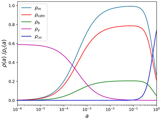
Since we aim to solve the system of Equations (4) and (5), with the constraint Equation (6) and using class [29], we write in Appendix A the corresponding class equations, in which we make use of the conformal and cosmic times, as well as the number-of-e-folds parameter $N(\equiv$$\ln a)$. The last term of Equation (4) (or class version A6) decreases towards the past for $n>0$ but diverges for $n<0$; however, in a matter- or radiation-dominated universe, the energy density diverges too as ${\rho }_{dm}$∼$1/{\eta }^6$ and ${\rho }_{\gamma }$∼$1/{\eta }^4$, respectively. Thus, the final result for n should not diverge faster than $n=-4$ to maintain our CHDE model as subdominant in these Universes’ eras, only becoming dominant at later times, $z<1$. In Figure 1, we show the densities’ evolution, demonstrating the mentioned behavior, where we observe the decrease in dark matter, steeper than baryons, and the rise of dark energy as time evolves.

Figure 1. Density parameter evolution as a function of the scale factor.

We now clarify the perturbative prescription adopted in this work. The standard perturbation equations are retained for photons, baryons, and neutrinos, while the dark-matter continuity equation includes the interaction term derived below. The metric perturbations evolve consistently with these components and the modified background. The background continuity equation alone does not uniquely determine the perturbations: a covariant prescription for the energy transfer is also required [18]. We adopt the covariant energy-transfer prescription

$$Q_{\mu }=Q{u}_{\mu }^{\left(dm\right)},$$

(7)

i.e., the energy flow is parallel to the dark-matter four-velocity. This choice implies that there is no momentum transfer in the dark-matter rest frame. In our case,

$$T_{\mathcal{M}\nu }^{\mu }=-{\rho }_{\mathcal{M}}{{\delta }^{\mu }}_{\nu }.$$

(8)

In particular, the gauge-invariant CHDE density perturbation on hypersurfaces comoving (com) with dark matter satisfies

$$\delta {\rho }_{\mathcal{M},\mathrm{com}}=\delta {\rho }_{\mathcal{M}}+{\rho }_{\mathcal{M}}^{\prime }{\theta }_{dm}=0.$$

(9)

Hence, in the dark-matter-comoving synchronous gauge,

$${\theta }_{dm}=0,\delta {\rho }_{\mathcal{M}}=0.$$

(10)

The CHDE component therefore introduces no independent propagating scalar degree of freedom in this prescription. Nevertheless, the interaction modifies the evolution of the fractional dark-matter density contrast through the time dependence of the background dark-matter density. For pressureless dark matter, the perturbed conservation equation of Ref. [18] reduces, in the dark-matter-comoving synchronous gauge, to 

$$\delta {\rho }_{dm}^{\prime }+3\mathcal{H}\delta {\rho }_{dm}+{\displaystyle \frac{1}{2}}{\rho }_{dm}{h}^{\prime }=0,$$

(11)

where h is the usual scalar metric perturbation in the synchronous gauge. Introducing the fractional contrast

$${\delta }_{dm}\equiv {\displaystyle \frac{\delta {\rho }_{dm}}{{\rho }_{dm}}},$$

(12)

and using Equation (5), one obtains

$${\delta }_{dm}^{\prime }=-{\displaystyle \frac{h^{\prime }}{2}}+{\displaystyle \frac{{\rho }_{\mathcal{M}}^{\prime }}{{\rho }_{dm}}}{\delta }_{dm}.$$

(13)

For the CHDE density, this becomes

$${\delta }_{dm}^{\prime }=-{\displaystyle \frac{h^{\prime }}{2}}+{\displaystyle \frac{n{\rho }_{\mathcal{M}}}{\eta {\rho }_{dm}}}{\delta }_{dm}.$$

(14)

Thus, although the CHDE density perturbation itself vanishes in the dark-matter-comoving synchronous gauge, the vacuum–dark-matter energy exchange changes the growth of the dark-matter density contrast. All other standard species are evolved with their usual perturbation equations. In the limit $n=0$, one has ${\rho }_M^{\prime }=0$, and Equation (14) reduces to the standard CDM result ${\delta }_{dm}^{\prime }=-h^{\prime }/2$. In Appendix A, we include the perturbed Equation (A5).

3. Cosmological Data and Model Testing

3.1. Cosmological Data

We implement the CHDE model in class [29] and perform Bayesian parameter inference through Markov chain Monte Carlo sampling with Cobaya [30]. The observational datasets and their implementation are summarized below.

• DESI DR2 BAO. We use the compressed baryon acoustic oscillation measurements from DESI Data Release 2 [7], or BAO for short. These constrain combinations of the transverse comoving distance $D_M\left(z\right)$, the radial distance $D_H\left(z\right)=c/H\left(z\right)$, and the volume-averaged distance $D_V\left(z\right)={\left[z{D}_M^2\left(z\right)D_H\left(z\right)\right]}^{1/3}$, expressed relative to the sound horizon at the baryon drag epoch, $r_d$. We employ the public DESI DR2 BAO likelihood implemented in Cobaya, with the released compressed distance measurements and their covariance matrix, including statistical and systematic uncertainties [7]. The likelihood is taken to be multivariate Gaussian,

  $$-2\ln {\mathcal{L}}_{\mathrm{BAO}}=\Delta {\mathbf{d}}^T{\mathbf{C}}_{\mathrm{BAO}}^{-1}\Delta \mathbf{d}+\mathrm{const}.,$$

  (15)

  where $\Delta \mathbf{d}={\mathbf{d}}_{\mathrm{th}}-{\mathbf{d}}_{\mathrm{obs}}$ and the theoretical distance ratios are computed with our modified CLASS code.
• Planck CMB. We employ the multipole CamSpec likelihood (version 12.6), based on the Planck PR4/NPIPE maps, using the combined $TT$, $TE$, and $EE$ spectra [31,32]. The theoretical spectra are computed with the modified CLASS code, including the CHDE background evolution and the perturbation prescription described in Section 2.
• ACT lensing. We include the ACT Data Release 6 (DR6) CMB lensing reconstruction [33,34,35]. This dataset constrains the angular power spectrum of the CMB lensing potential, $C_L^{\varphi \varphi }$, providing information on the intervening matter distribution and its growth. We use the public ACT DR6 CMB lensing likelihood, adopting the ACT-only baseline reconstruction, which combines temperature and polarization information. The likelihood assumes Gaussian errors for ten lensing power-spectrum bandpowers over $40<L<763$ and uses the released simulation-based covariance matrix.
• Pantheon+. This compilation combines standardized Type Ia supernova light curves from several surveys [10,11]. We use the Pantheon+ compilation implemented through the standard sn.pantheonplus likelihood in Cobaya. We select objects with Hubble-diagram redshifts $z_{\mathrm{HD}}>0.01$ and adopt the released covariance matrix including statistical and systematic uncertainties, restricted to the selected sample. The likelihood is Gaussian in the corrected apparent-magnitude residuals, with the absolute-magnitude normalization analytically marginalized. We do not include the SH0ES Cepheid calibration.
• Union3. Union3 combines Type Ia supernova observations analyzed with the UNITY1.5 Bayesian hierarchical framework [12]. We use the compressed Union3 distance measurements derived with the UNITY1.5 Bayesian hierarchical framework. We employ the standard sn.union3 likelihood in Cobaya, which compares the released distance–redshift relation with the luminosity distances predicted by the CHDE model. The likelihood adopts a multivariate Gaussian approximation with the supplied covariance matrix, incorporating statistical and systematic uncertainties and correlations between the compressed distance measurements. The overall distance normalization is analytically marginalized, so no external absolute-magnitude calibration is imposed.
• DES Year 5. We use the DES Year 5 supernova sample [13], comprising 1635 photometrically classified supernovae in the range $0.10<z<1.13$, together with 194 external low-redshift Type Ia supernovae at $0.025<z<0.10$. We adopt the released cosmological sample without additional selection cuts and employ the standard sn.desy5 likelihood in Cobaya. The likelihood is Gaussian in the distance-modulus residuals relative to the CHDE prediction. Its covariance combines the released systematic covariance matrix with the diagonal statistical variances supplied with the distance measurements. The overall magnitude normalization is analytically marginalized, without imposing an external absolute-magnitude calibration.

For the supernova datasets, the predicted distance modulus is

$${\mu }_{\mathrm{th}}\left(z\right)=5{\log }_{10}\left[{\displaystyle \frac{D_L\left(z\right)}{\mathrm{Mpc}}}\right]+25,$$

(16)

where $D_L\left(z\right)$ is the luminosity distance in the CHDE cosmology. Pantheon+, Union3, and DES Year 5 are considered as alternative supernova compilations, rather than combined into a single supernova likelihood. The dataset combinations used in each analysis are specified in sets A–E below.

3.2. Model Testing

To understand the role of the new DE model, we performed different parameter inferences, one with fixed massive neutrinos to $0.06$ eV (a single massive and two massless neutrinos) and the other with $\sum m_{\nu }$ as a free parameter. We also run inferences for a flat Universe and for curvature as a free parameter (again with a single massive neutrino). The inclusion of massive neutrinos and curvature as free parameters is motivated by the recent debate regarding the negative mass posterior probability [21,36,37] and curvature as a possible solution to this issue [22].

We opted to use the same priors as in the DESI BAO DR2 cosmological analysis [7] in order to compare their results for the ΛCDM model with ours for the CHDE model. Our priors are displayed in Table 1, where we also vary the CHDE exponent n; see Equation (3). The CHDE strength parameter Q (or ${\mathrm{\Omega }}_{\mathcal{M}}^{\left(0\right)}$) is a derived parameter obtained from the constraint Equation (6), similar, as it happens, in the ΛCDM model to determine ${\mathrm{\Omega }}_{\mathrm{\Lambda }}$.

Table 1. Priors of the relevant fitting parameters. Here, $\mathcal{U}$ and $\mathcal{G}$ denote uniform and Gaussian priors, respectively.

Parameters	Priors
$n$	$\mathcal{U}(-1,1)$
${\mathrm{\Omega }}_k$	$\mathcal{U}(-0.3,0.3)$
$H_0$ [km/s/Mpc]	$\mathcal{U}(20,150)$
${\omega }_{\mathrm{b}}$	$\mathcal{G}(0.0222,0.{0005}^2)$
${\omega }_{\mathrm{cdm}}$	$\mathcal{U}(0.001,0.99)$
$\ln \left({10}^{10}{A}_s\right)$	$\mathcal{U}(1.61,3.91)$
$n_{\mathrm{s}}$	$\mathcal{U}(0.8,1.2)$
${\tau }_{\mathrm{reio}}$	$\mathcal{U}(0.01,0.8)$
$\sum m_{\nu }$ [eV]	$\mathcal{U}(0,5)$

For the analysis, we consider the following set of data and models:

(A)

Individual data of DESI BAO DR2, Planck, Pantheon+, DESY5, and Union3. For these datasets, we perform the inference, allowing spatial curvature to vary while keeping the neutrino mass fixed, since, when treated as a free parameter, it is better constrained with the ACT lensing information that will be included in the subsequent datasets. Results of this set are in Table 2.

Table 2. Parameter inference for the relevant cosmological parameters using independent BAO DESI DR2, Planck, and SNe Ia data. Results correspond to set A, as explained in the main text.

	BAO	Planck	Pantheon+	DESY5	Union3
Parameter	68% Limits	68% Limits	68% Limits	68% Limits	68% Limits
n	$-0.{15}_{-0.37}^{+0.31}$	$-0.312\pm 0.056$	$-0.{28}_{-0.49}^{+0.30}$	$-0.{41}_{-0.50}^{+0.22}$	$-0.{40}_{-0.55}^{+0.18}$
${\mathrm{\Omega }}_k$	$0.{107}_{-0.10}^{+0.069}$	$-0.{0041}_{-0.0068}^{+0.0060}$	$0.{149}_{-0.077}^{+0.11}$	$0.{151}_{-0.075}^{+0.10}$	$0.{148}_{-0.078}^{+0.098}$
${\mathrm{\Omega }}_{\mathrm{b}}{h}^2$	$0.02222\pm 0.00050$	$0.{02226}_{-0.00017}^{+0.00041}$	$0.02222\pm 0.00050$	$0.02222\pm 0.00050$	$0.02223\pm 0.00050$
${\mathrm{\Omega }}_{\mathrm{m}}$	$0.{302}_{-0.025}^{+0.033}$	$0.{374}_{-0.048}^{+0.023}$	$0.318\pm 0.024$	$0.344\pm 0.022$	$0.352\pm 0.032$
$H_0\left[\mathrm{km}{\mathrm{s}}^{-1}{\mathrm{Mpc}}^{-1}\right]$	$73.7_{-7.5}^{+4.6}$	$66.7\pm 3.5$	${108}_{-40}^{+40}$	${109}_{-40}^{+40}$	${109}_{-40}^{+40}$
${\mathrm{\Omega }}_{\mathcal{M}}$	$0.{592}_{-0.073}^{+0.12}$	$0.{630}_{-0.019}^{+0.045}$	$0.533\pm 0.084$	$0.505\pm 0.082$	$0.{500}_{-0.094}^{+0.085}$

(B)

DESI BAO DR2 + SNe Ia for a model with free curvature and a fixed neutrino mass, as in A, but now we use two datasets for the inference. Results of this set are in Table 3.

Table 3. Results for the joint analysis of BAO DR2 + SNe Ia data. Results from set B.

	BAO-Pantheon+	BAO-DESY5	BAO-Union3
Parameter	68% Limits	68% Limits	68% Limits
n	$-0.30\pm 0.24$	$-0.52\pm 0.24$	$-0.44\pm 0.28$
${\mathrm{\Omega }}_k$	$0.{129}_{-0.10}^{+0.080}$	$0.156\pm 0.078$	$0.146\pm 0.081$
${\mathrm{\Omega }}_{\mathrm{b}}{h}^2$	$0.02222\pm 0.00050$	$0.02223\pm 0.00050$	$0.02223\pm 0.00050$
${\mathrm{\Omega }}_{\mathrm{m}}$	$0.314\pm 0.019$	$0.332\pm 0.017$	$0.326\pm 0.021$
$H_0$ [km/s/Mpc]	$75.0_{-7.9}^{+6.2}$	$74.3_{-8.0}^{+6.9}$	$74.4_{-8.0}^{+6.7}$
${\mathrm{\Omega }}_{\mathcal{M}}$	$0.{556}_{-0.073}^{+0.10}$	$0.511\pm 0.081$	$0.528\pm 0.086$

(C)

DESI BAO DR2 + Planck data + SNe Ia for a model with free curvature and a fixed neutrino mass, as in A, but now we use three datasets for the inference. Results of this set are in Table 4.

Table 4. Results for the joint analysis employing BAO DR2 + Planck + SNe Ia data. Results from set C.

	BAO-Pantheon+-Planck	BAO-DESY5-Planck	BAO-Union3-Planck
Parameter	68% Limits	68% Limits	68% Limits
n	$-0.285\pm 0.061$	$-0.284\pm 0.052$	$-0.280\pm 0.054$
${\mathrm{\Omega }}_k$	$0.{0027}_{-0.0033}^{+0.0016}$	$0.{0021}_{-0.0024}^{+0.0015}$	$0.{0023}_{-0.0024}^{+0.0016}$
${\mathrm{\Omega }}_{\mathrm{b}}{h}^2$	$0.{02250}_{-0.00015}^{+0.00018}$	$0.02249\pm 0.00016$	$0.02248\pm 0.00016$
${\mathrm{\Omega }}_{\mathrm{m}}$	$0.{3295}_{-0.0076}^{+0.0066}$	$0.3304\pm 0.0063$	$0.{3296}_{-0.0070}^{+0.0062}$
$H_0$ [km/s/Mpc]	$70.{75}_{-1.2}^{+0.81}$	$70.{43}_{-0.85}^{+0.74}$	$70.{43}_{-0.87}^{+0.70}$
${\mathrm{\Omega }}_{\mathcal{M}}$	$0.{6678}_{-0.0068}^{+0.0096}$	$0.{6674}_{-0.0063}^{+0.0074}$	$0.{6680}_{-0.0064}^{+0.0081}$

(D)

DESI BAO DR2 + Planck + ACT + Union3 SNe Ia for both curvature and neutrino mass as free parameters. Results of this set are in Table 5.

Table 5. Results for the joint analysis employing Planck + ACT DR6 and BAO DR2 + Planck + ACT DR6 data for a non-flat model. Neutrino masses are given in eV and reported with 95% C.L., as standard. Results from set D.

	Planck-ACT	BAO-Planck-ACT	BAO-Union3-Planck-ACT
Parameter	68% Limits	68% Limits	68% Limits
n	$-0.321\pm 0.080$	$-0.279\pm 0.064$	$-0.239\pm 0.072$
${\mathrm{\Omega }}_k$	$-0.0176\pm 0.0079$	$0.{0038}_{-0.0022}^{+0.0017}$	$0.{0032}_{-0.0018}^{+0.0015}$
${\mathrm{\Omega }}_{\mathrm{b}}{h}^2$	$0.02215\pm 0.00016$	$0.02220\pm 0.00013$	$0.02219\pm 0.00013$
${\mathrm{\Omega }}_{\mathrm{m}}$	$0.{462}_{-0.059}^{+0.050}$	$0.3344\pm 0.0086$	$0.3310\pm 0.0091$
$H_0$	$57.8\pm 3.4$	$67.68\pm 0.39$	$67.70\pm 0.40$
${\mathrm{\Omega }}_{\mathcal{M}}$	$0.{556}_{-0.044}^{+0.052}$	$0.6618\pm 0.0096$	$0.{666}_{-0.0098}^{+0.011}$
$\sum m_{\nu }$ [eV]   (95% C.L.)	$0.{34}_{-0.30}^{+0.34}$	$0.{037}_{-0.052}^{+0.070}$	$0.{033}_{-0.044}^{+0.062}$

(E)

DESI BAO DR2 + Planck + ACT + Union3 SNe Ia for a flat model and a free neutrino parameter. Results of this set are in Table 6.

Table 6. Results for the joint analysis employing Planck + ACT DR6 and BAO DR2 + Planck + ACT DR6 data for a flat model. Neutrino masses are given in eV and reported with 95% C.L., as standard. Results from set E.

	Planck-ACT	BAO-Planck-ACT	BAO-Union3-Planck-ACT
Parameter	68% Limits	68% Limits	68% Limits
n	$-0.322\pm 0.074$	$-0.{279}_{-0.052}^{+0.065}$	$-0.{262}_{-0.11}^{+0.089}$
${\mathrm{\Omega }}_{\mathrm{b}}{h}^2$	$0.{02196}_{-0.00017}^{+0.00021}$	$0.02233\pm 0.00012$	$0.02231\pm 0.00012$
${\mathrm{\Omega }}_{\mathrm{m}}$	$0.{412}_{-0.054}^{+0.036}$	$0.{3327}_{-0.0086}^{+0.0073}$	$0.{3320}_{-0.011}^{+0.0062}$
$H_0$	$61.9_{-2.4}^{+3.3}$	$67.40\pm 0.36$	$67.{37}_{-0.33}^{+0.38}$
${\mathrm{\Omega }}_{\mathcal{M}}$	$0.{588}_{-0.036}^{+0.054}$	$0.{6672}_{-0.0073}^{+0.0086}$	$0.{668}_{-0.0062}^{+0.011}$
$\sum m_{\nu }$ [eV]   (95% C.L.)	$0.{39}_{-0.39}^{+0.46}$	$0.{021}_{-0.029}^{+0.040}$	$0.{018}_{-0.024}^{+0.033}$

We clarify that Pantheon+, Union3, and DES Year 5 are treated as alternative supernova datasets and are analyzed separately. We never combine two or more of these compilations within the same likelihood. For each analysis involving supernovae, we include only one compilation, either alone or together with the BAO and CMB datasets specified in sets A–E. In particular, the neutrino-mass analyses in sets D and E use Union3 as their sole supernova dataset.

For each compilation, we evaluate its respective Cobaya likelihood using the CHDE luminosity-distance prediction and the corresponding covariance matrix, including statistical and systematic uncertainties. The overall magnitude normalization is analytically marginalized. For a joint analysis, the selected supernova likelihood is multiplied by the likelihoods of the other cosmological probes included in that dataset combination.

We emphasize that the BAO likelihoods used in this work correspond to compressed distance measurements and therefore constrain the background distance–redshift relation and the sound-horizon scale. The CMB likelihoods, on the other hand, require the Boltzmann evolution of the cosmological perturbations in the modified CHDE background. In  particular, for the analyses including massive neutrinos, where the inferred neutrino-mass constraints may be especially sensitive to the evolution of cosmological perturbations, we implement the covariant energy-transfer prescription for the CHDE–dark-matter sector described above. In the dark-matter-comoving synchronous gauge, the CHDE component carries no independent density perturbation, while the dark-matter continuity equation is modified by the energy exchange with the CHDE component. The perturbations of all other standard cosmological species, including massive neutrinos, as well as the metric perturbations, are evolved consistently within the Boltzmann calculation.

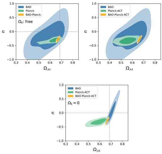
The inferred cosmological parameters are summarized in the following tables and figures. Our results report best-fitted parameters with $68\%$ confidence levels (C.L.), except  for $\Sigma m_{\nu }$, for which we report $95\%$ C.L. Table 2 presents the results obtained for dataset A. We analyze each dataset separately to characterize their constraining power and parameter degeneracies within CHDE, assess consistency between probes, and identify their contributions to the joint constraints. In particular, uncalibrated supernova distances constrain the shape of the distance–redshift relation but do not independently determine $H_0$. The broad, prior-dependent $H_0$ intervals from supernova-only analyses should be interpreted accordingly. Independent analyses of BAO and SNe Ia allow for a relatively broad range of parameter values within our model, indicating that the CHDE scenario remains partially consistent with the standard ΛCDM model, which is recovered for the specific parameter choices (${\mathrm{\Omega }}_{\mathcal{M}}^{\left(0\right)}={\mathrm{\Omega }}_{\mathrm{\Lambda }},n=0$). However, results from Planck data alone exclude ΛCDM. Also, the joint analysis of BAO and SNe Ia displayed in Table 3 disfavors the ΛCDM model. Next, Table 4 reports the parameter constraints derived from the combined BAO + Planck + SNe Ia data. In this case, the  ΛCDM model is disfavored with even greater statistical precision: the non-flat model is disfavored by 4.4$\sigma$, whereas the flat model is $4.5\sigma$ away from ΛCDM1. These results are presented more visually in Figure 2, which shows contour plots for the best-fitted parameters of the model (${\mathrm{\Omega }}_{\mathcal{M}}^{\left(0\right)}$, n) for the analysis combining the different sets. The joint analysis clearly excludes the ΛCDM model (dashed lines) as the best fit. Note that the apparent position of the joint BAO+CMB contour should be interpreted with some care, since it is obtained from the full multidimensional joint likelihood and then projected onto the $({\mathrm{\Omega }}_{\mathcal{M}}^{\left(0\right)},n)$ plane. Therefore, it does not necessarily coincide with the visual overlap of the independently marginalized BAO and CMB contours.

Figure 2. Contour plots of the CHDE model parameters: The dark energy density parameter ${\mathrm{\Omega }}_{\mathcal{M}}^{\left(0\right)}$ and the power-law exponent n, cf. Equation (3). The left panel shows BAO, Planck, and BAO + Planck constraints with curvature as a free parameter. The upper-right panel shows BAO, Planck + ACT, and BAO + Planck + ACT constraints, also allowing curvature to vary. The lower panel shows the corresponding BAO, Planck + ACT, and BAO + Planck + ACT constraints for the flat model. Our results exclude the ΛCDM limit, ${\mathrm{\Omega }}_{\mathcal{M}}^{\left(0\right)}={\mathrm{\Omega }}_{\mathrm{\Lambda }}$ and $n=0$, as the best-fit solution when CMB data are included.

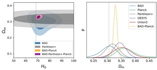
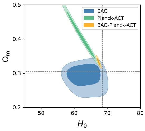
As it happens in the ΛCDM model, ${\mathrm{\Omega }}_m$ is smaller for BAO than for Planck, but the discrepancy is larger in our CHDE model. Figure 3 shows the matter density parameter vs the Hubble constant (left panel) and one-dimensional (1D) marginalized posteriors when using different datasets (right panel). Also, in this figure, one observes a shift in the value of the Hubble constant towards larger values than in ΛCDM (vertical dashed line). The reported value in Table 4 for BAO–Planck–Pantheon+ data is $H_0=70.{75}_{-1.2}^{+0.81}$ km${\mathrm{s}}^{-1}$${\mathrm{Mpc}}^{-1}$ when ${\mathrm{\Omega }}_k$ is a free parameter, whereas in ΛCDM, it is $63.3\pm 2.1$ km${\mathrm{s}}^{-1}$${\mathrm{Mpc}}^{-1}$ [7]. For a flat cosmology, we report in Table 6 a value of $67.40\pm 0.36$ km${\mathrm{s}}^{-1}$${\mathrm{Mpc}}^{-1}$, and the ΛCDM for the Planck data is $67.36\pm 0.54$ km${\mathrm{s}}^{-1}$${\mathrm{Mpc}}^{-1}$ [38], compatible values to 1$\sigma$. These results are shown in Figure 4. Thus, the results for $H_0$ do not solve the Hubble tension using early universe physics (CMB and BAO).

Figure 3. Contour plots of matter density parameter vs. the Hubble constant for the CHDE model (left) and the marginalized 1D posteriors probabilities (P) for different datasets (right). As a reference, the black dashed line points to the best-fit values for the ΛCDM model using Planck data.

Figure 4. Contour plots of matter density parameter vs the Hubble constant for the flat CHDE model. As a reference, the black dashed line points to the best-fit values for the ΛCDM model using Planck data.

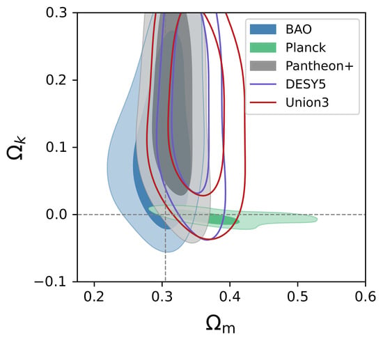
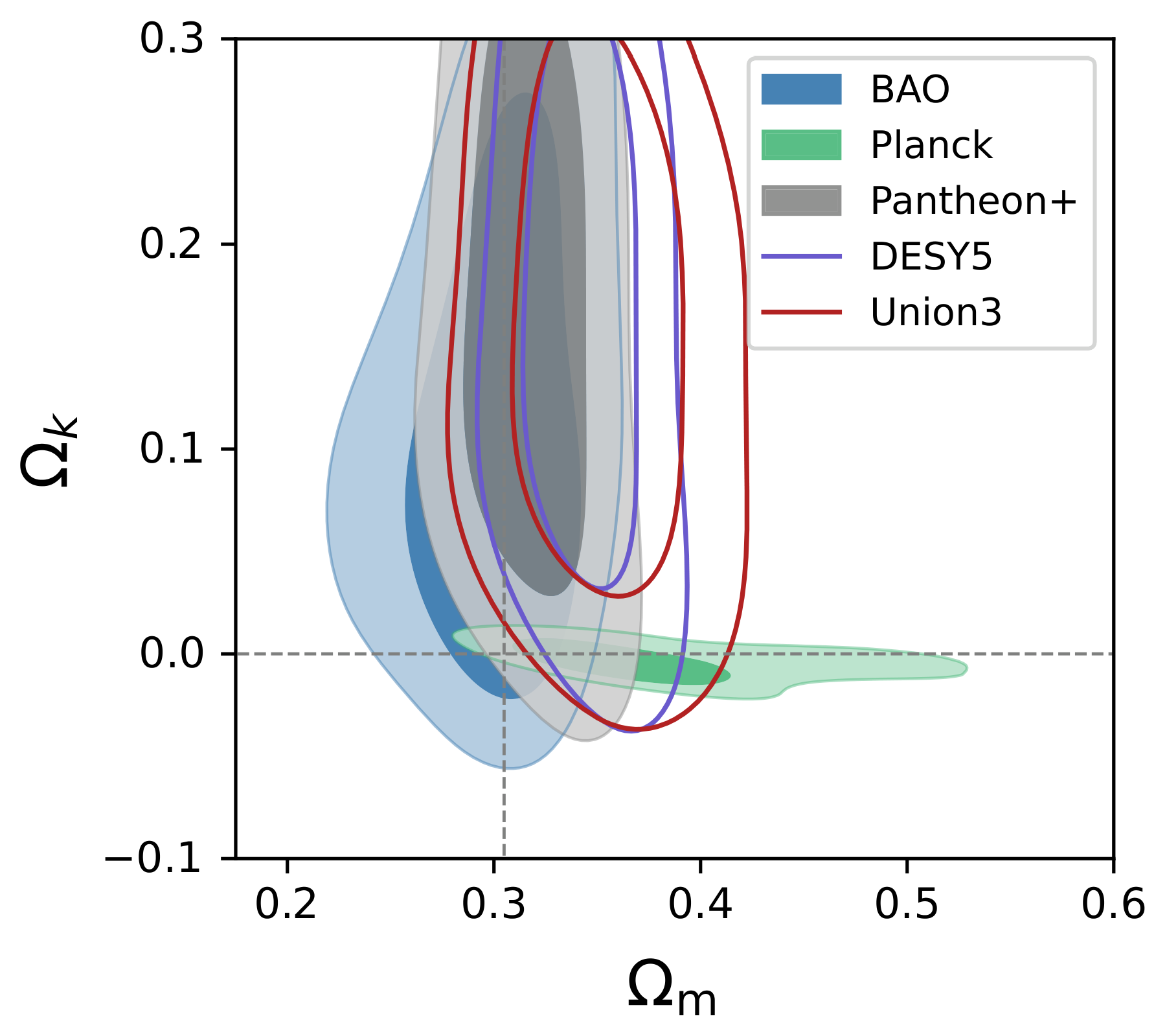
With runs A–D, we explore the role of curvature in our CHDE model. The curvature behaves similar to the ΛCDM model’s: Planck fitting results in a small negative ${\mathrm{\Omega }}_k$ [32], whereas DESI BAO fitting favors a positive value [7], although in our case, ${\mathrm{\Omega }}_k$ is larger and has greater uncertainties, since we include an additional parameter. These results are shown in Table 2, and  Figure 5 shows the contour plots of the curvature vs. the matter parameter. Further fittings that include BAO data in Table 3, Table 4 and Table 5 show a preference for a positive ${\mathrm{\Omega }}_k$. The low $H_0$ values inferred from Planck + ACT illustrate the model dependence of the CMB-based determination of the present expansion rate. The modified CHDE evolution, together with free neutrino mass and spatial curvature where applicable, permits parameter combinations with low $H_0$ and higher matter density. Since low $H_0$ also occurs in the flat analysis, curvature is not the sole explanation. Adding BAO constrains the distance–redshift relation at several epochs, restricts these degeneracies, and shifts the posterior toward higher $H_0$ with smaller uncertainties. We do not attribute this shift to a specific observational systematic.

Figure 5. Contour plots of the curvature and matter density parameters for the CHDE model.

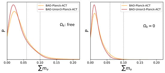
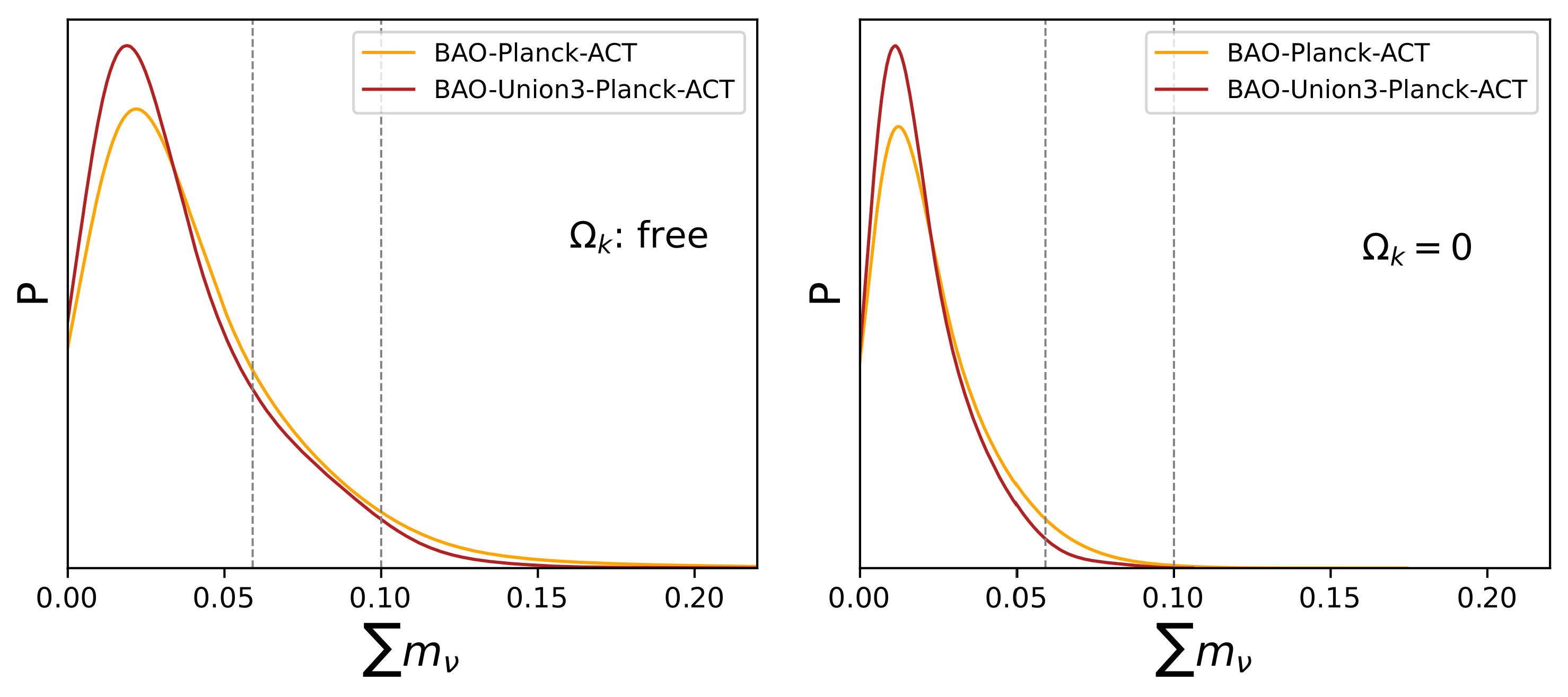
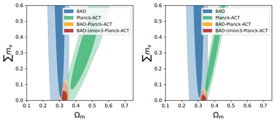
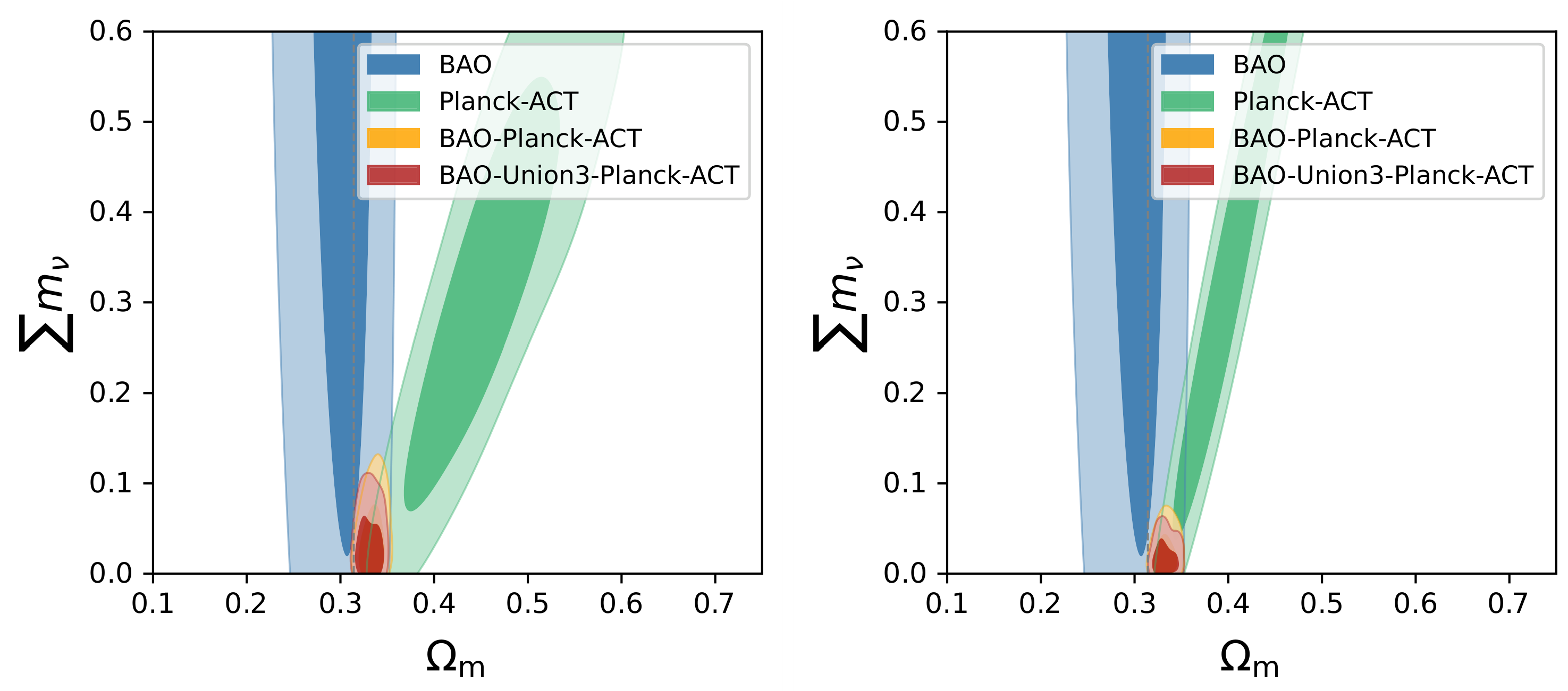
In recent determinations of the summed neutrino mass ($\sum m_{\nu }$), the DESI collaboration reports very small values that may eventually come into tension with terrestrial oscillation experiments, which establish a lower bound on this quantity of $\sum m_{\nu }>0.059$ eV for normal mass hierarchy (NH) and $\sum m_{\nu }>0.1$ eV for inverted hierarchy (IH) [39]. The result found in the DESI DR2 analysis is, for a flat cosmology, $\sum m_{\nu }<0.0642$ eV ($95\%$ C.L.) [7], and SPT-3G D1 + DESI and CMB-SPA + DESI combinations appear to rule out the normal and inverted hierarchies at $97.9\%$ and $99.9\%$ confidence, respectively [40]. Furthermore, the maximum posterior probability lies at nonphysical, negative values [21]. These conflicting results open the possibility for alternative scenarios. In this sense, reference [22] argues that inclusion of the curvature as a free parameter relaxes the constraint to $\sum m_{\nu }<0.1$ eV ($95\%$ C.L.) and makes the posterior probability more positive, suggesting that curvature may alleviate the problem. However, their maximum probability is around zero, suggesting that a full resolution would require performing an analysis with effective negative neutrino masses [21,23]. In our CHDE model, we compute the neutrino mass using sets D (free curvature) and E (flat model), obtaining the results in Table 5 and Table 6: we obtain $\sum m_{\nu }=0.{34}_{-0.30}^{+0.34}$ eV ($95\%$ C.L.) with a negative ${\mathrm{\Omega }}_k$ when using Planck + ACT data, and $\sum m_{\nu }=0.{037}_{-0.052}^{+0.070}$ eV ($95\%$ C.L.) with BAO+Planck+ACT data, resulting in a positive ${\mathrm{\Omega }}_k$ as in ref. [22]; in addition, we performed the inference including the Union3 SNe Ia dataset, since supernovae are known to shift the neutrino mass toward negative values. We find that in the CHDE model, the neutrino mass remains positive, with a significance similar to that obtained with the previous datasets. For a flat cosmology, we obtain $\sum m_{\nu }=0.{39}_{-0.39}^{+0.46}$ eV ($95\%$ C.L.) when using Planck+ACT data, and $\sum m_{\nu }=0.{021}_{-0.029}^{+0.040}$ eV ($95\%$ C.L.) with BAO + Planck + ACT data; we further include the Union3 SNe Ia dataset and find similar results, with the neutrino mass remaining positive. All these results are compatible with the terrestrial oscillation experiment constraints within $95\%$ C.L. Furthermore, Figure 6 depicts the marginalized 1D posterior probabilities for non-flat and flat models, clearly showing that, in both cases, the maximum lies at positive values of $\sum m_{\nu }$ in the CHDE model. The flat ΛCDM model provides a clearer indication against the inverted hierarchy (IH). On the other hand, as discussed above, DESI data favor a lower value of ${\mathrm{\Omega }}_m$ than Planck data. This mismatch reduces the overlap between the parameter regions preferred by the two datasets when they are combined, particularly in the $\sum m_{\nu }$ direction. Figure 7 shows these results for both flat and non-flat models. The concordance region, where the probability contours overlap, is relatively small, which drives the combined constraint toward a small value of $\sum m_{\nu }$. We caution that the perturbation model used here is a particular one, and that different perturbation settings can change the neutrino mass results, as shown in ref. [41].

Figure 6. Posterior probabilities of the sum of the neutrino masses for non-flat (left panel) and flat (right panel) models for the CHDE model. Both plots show a maximum probability in the positive neutrino masses. For reference, vertical dashed lines indicate the NH and IH experimental limits from terrestrial experiments, at $0.059$ eV and $0.1$ eV, respectively.

Figure 7. Contour plots of the neutrino mass vs the matter density parameter. The left panel is for ${\mathrm{\Omega }}_k$ as a free parameter, and the right panel for a flat model. The region of concordance in the joint analysis is quite narrow, driving the inferred neutrino mass towards very small values.

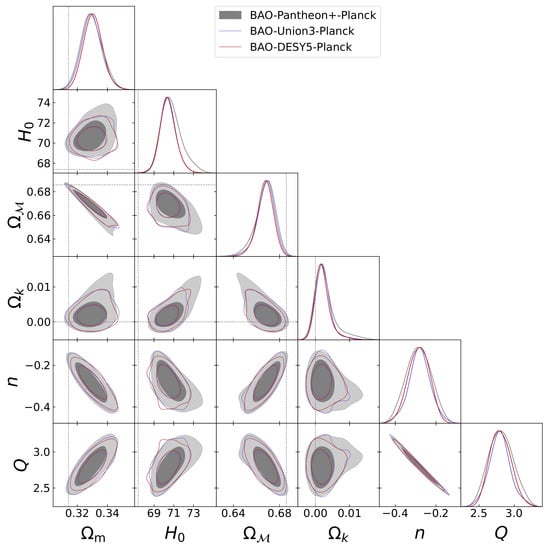
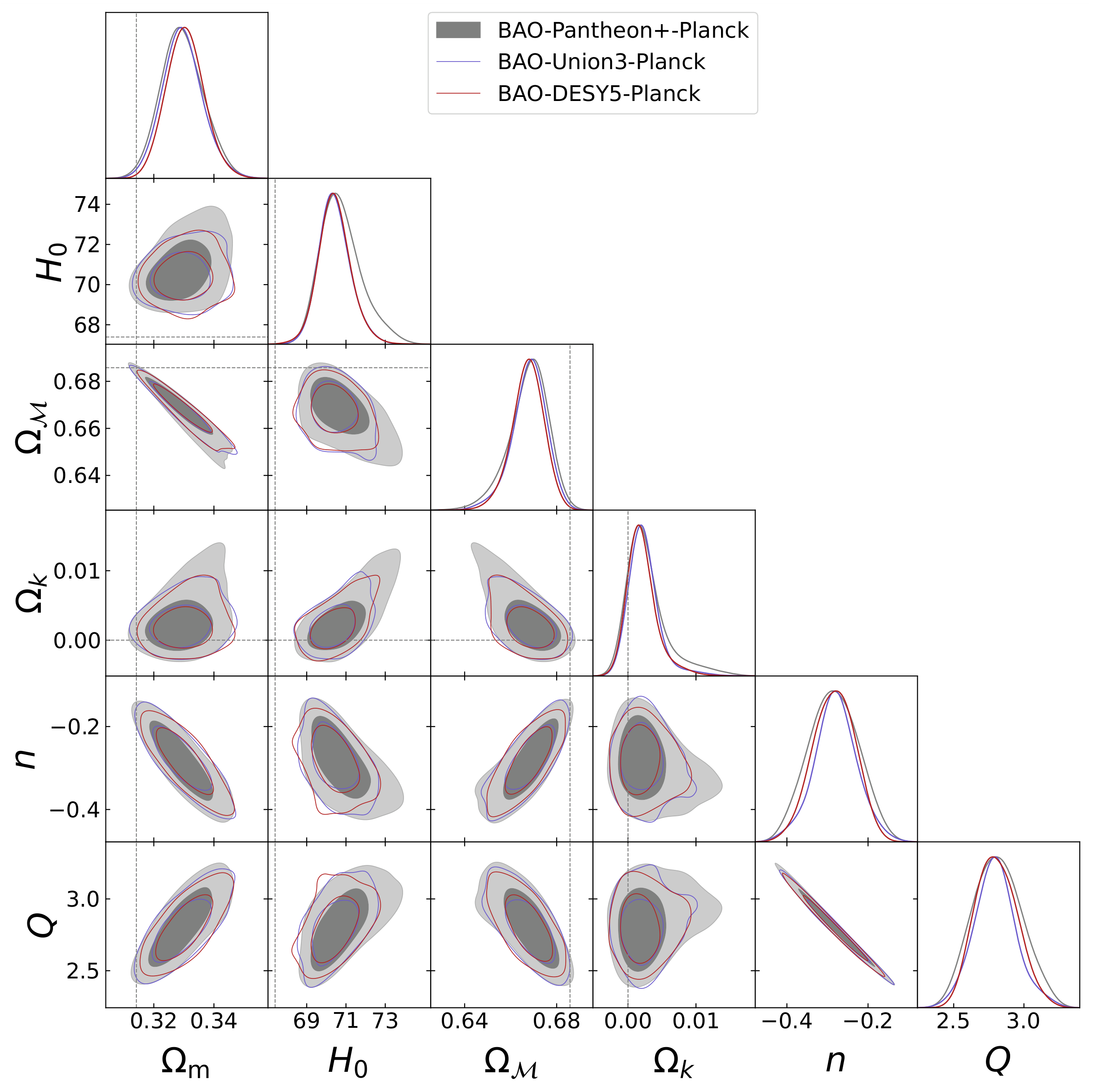
Figure 8, Figure 9 and Figure 10 present the marginalized posterior distributions and joint constraints on the cosmological parameters for sets C–E. Figure 8 shows the results for set C, in which spatial curvature varies and the summed neutrino mass is fixed to $0.06\mathrm{eV}$. The different BAO + Planck + SNe Ia combinations yield mutually consistent constraints, with a preference for a negative CHDE exponent n and a small positive curvature parameter ${\mathrm{\Omega }}_k$. Each combination includes only one supernova compilation.

Figure 8. Contour plots of the relevant parameters for the CHDE model using set C with a free curvature model.

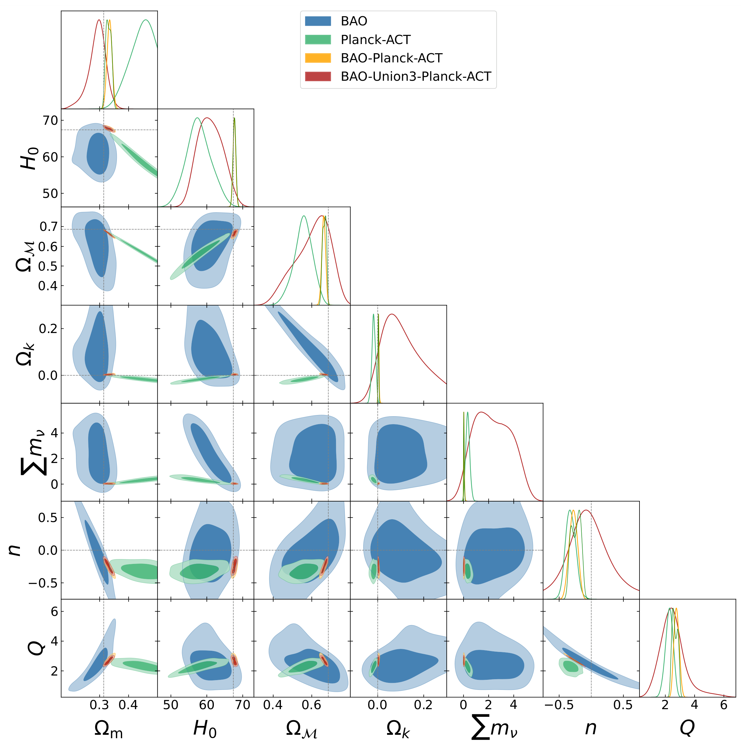
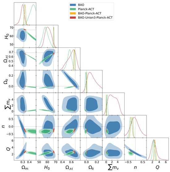
Figure 9. Contour plots of the relevant parameters for the CHDE model using set D with a free curvature model and free neutrino mass.

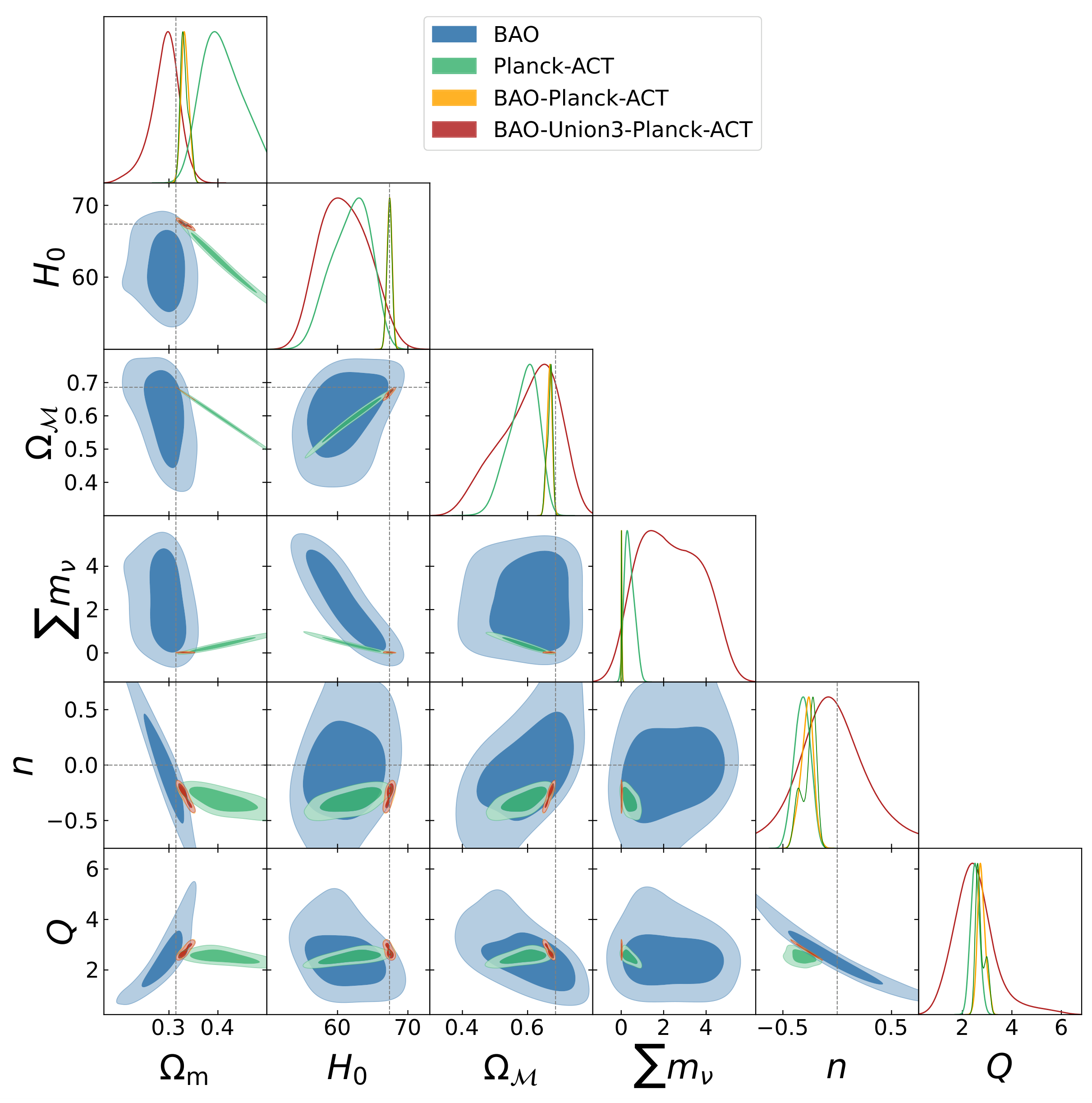
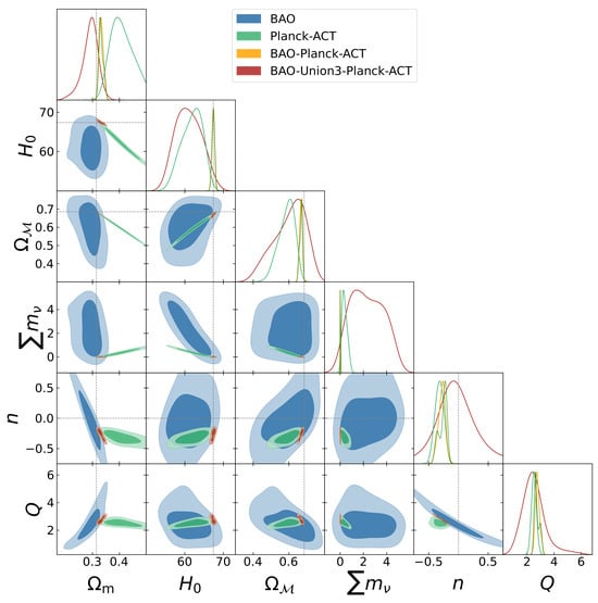
Figure 10. Contour plots of the relevant parameters for the CHDE model using set E for a flat model and free neutrino mass.

Figure 9 presents the results for set D, allowing both spatial curvature and the summed neutrino mass to vary. The comparison between Planck + ACT and the combinations including BAO illustrates the substantial tightening and shifting of the parameter constraints when BAO information is included, particularly for ${\mathrm{\Omega }}_m$, $H_0$, ${\mathrm{\Omega }}_k$, and $\sum m_{\nu }$. Figure 10 shows the corresponding results for set E, which assumes spatial flatness while allowing the summed neutrino mass to vary. In both sets, adding BAO shifts the neutrino-mass constraints toward smaller values, while the further inclusion of Union3 produces comparatively modest changes. The full distributions complement the selected parameter projections discussed above by displaying the correlations and the dependence of the inferred constraints on the dataset combination and the assumed spatial geometry.

3.3. Goodness of Fit

Finally, to assess model performance beyond parameter estimation and compare their goodness of fit and statistical support, we computed three statistical metrics using the maximum a posteriori (MAP) solutions obtained with Cobaya’s BOBYQA optimizer. Specifically, we report $\Delta {\chi }_{\mathrm{MAP}}^2$, together with MAP-based estimates of the Akaike Information Criterion (AIC) and the Bayesian Information Criterion (BIC). We follow the expressions given in [42], but evaluate the likelihood at the MAP rather than at its maximum. Table 7 presents the results for the CHDE model with neutrinos, with and without spatial curvature, relative to the corresponding ΛCDM model. For each criterion $X_i$, we define $\Delta X_i\equiv X_i^{\mathrm{CHDE}}-X_i^{\mathrm{\Lambda }\mathrm{CDM}}$, so that negative values favor CHDE. The CHDE model with curvature provides a slightly better fit according to $\Delta {\chi }_{\mathrm{MAP}}^2$ and is mildly preferred by the ΔAIC, whereas the ΔBIC favors ΛCDM. The flat CHDE model provides a comparable fit to ΛCDM according to $\Delta {\chi }_{\mathrm{MAP}}^2$, while both the ΔAIC and ΔBIC favor ΛCDM.

Table 7. Goodness-of-fit comparison between CHDE and ΛCDM. Differences are CHDE minus ΛCDM.

Criterion	Difference	Assessment
With curvature
$\Delta {\chi }_{\mathrm{MAP}}^2$	$-2.161$	CHDE slightly better fit
$\Delta \mathrm{AIC}$	$-0.161$	CHDE slightly preferred
$\Delta \mathrm{BIC}$	$+7.05$	ΛCDM preferred
Without curvature
$\Delta {\chi }_{\mathrm{MAP}}^2$	$+0.056$	Essentially identical fits
$\Delta \mathrm{AIC}$	$+2.056$	ΛCDM preferred
$\Delta \mathrm{BIC}$	$9.262$	ΛCDM preferred

3.4. Physical Interpretation

The preference for negative n has a direct physical interpretation. Since ${\rho }_{\mathcal{M}}\propto {\eta }^n$, its conformal-time derivative is ${\rho }_{\mathcal{M}}^{\prime }=n{\rho }_{\mathcal{M}}/\eta$. Thus, for positive dark energy density and $n<0$, the CHDE density decreases as the Universe evolves. The dark-matter continuity equation,

$${\rho }_{\mathrm{dm}}^{\prime }+3\mathcal{H}{\rho }_{\mathrm{dm}}=-{\rho }_{\mathcal{M}}^{\prime }=-{\displaystyle \frac{n{\rho }_{\mathcal{M}}}{\eta }},$$

(17)

then contains a positive source term, describing energy transfer from CHDE to dark matter. Equivalently,

$${\left(a^3{\rho }_{\mathrm{dm}}\right)}^{\prime }=-a^3{\rho }_{\mathcal{M}}^{\prime }>0.$$

(18)

The dark-matter energy in a fixed comoving volume therefore increases. This does not necessarily imply that its physical density increases: expansion can still dilute dark matter, but less rapidly than the $a^{-3}$ scaling of a separately conserved pressureless component. The inferred negative exponent consequently identifies a decaying vacuum-like dark-energy component that sources dark matter while retaining $w_{\mathcal{M}}=-1$. Its fractional contribution can nevertheless grow and dominate at late times because the other components dilute more rapidly. In the limit $n=0$, the transfer vanishes and the standard ΛCDM evolution is recovered.

The interaction also affects dark-matter perturbations. In the dark-matter-comoving synchronous gauge, their fractional density contrast obeys

$${\delta }_{\mathrm{dm}}^{\prime }=-{\displaystyle \frac{h^{\prime }}{2}}+{\displaystyle \frac{n{\rho }_{\mathcal{M}}}{\eta {\rho }_{\mathrm{dm}}}}{\delta }_{\mathrm{dm}}.$$

(19)

For $n<0$, the interaction term opposes the growth of overdensities. In the adopted prescription, $\delta {\rho }_{\mathcal{M}}=0$ in this gauge, so the energy transfer increases the mean dark-matter density without a corresponding perturbed source, thereby diluting the fractional contrast. This contribution does not necessarily make ${\delta }_{\mathrm{dm}}$ decrease with time, since gravitational growth can still dominate. This dilution suggests a tendency toward suppressed matter clustering and a lower ${\sigma }_8$, potentially also reducing $S_8\equiv {\sigma }_8\sqrt{{\mathrm{\Omega }}_m/0.3}$, although the net effect depends on the coupled background and perturbation evolution, as well as the inferred cosmological parameters. A dedicated analysis of these quantities and growth-rate observables is left for future work.

4. Conclusions

The striking recent results put forward by the DESI collaboration [4,7] suggest an evolving DE component instead of a constant, motivating the exploration of alternative models for the background expansion. Furthermore, notable discrepancies were identified in the inferred values of the matter density parameter, for which DESI yields a lower value while Planck favors a higher one. Although the neutrino mass determined by DESI appears to be within the range allowed by oscillation experiments, the resulting posterior lies on the negative-mass side.

As an alternative to ΛCDM, we propose a model, the conformal holographic dark energy model, dubbed CHDE, in which dark energy depends on the conformal time through an exponent n, which can be constrained by observations; this represents an extra parameter with respect to the ΛCDM model. The model differs from the standard holographic formulation, but resembles the vacuum dark energy model [18]; its equation of state is $w_{DE}=-1$, but it includes an interaction between dark matter and dark energy through the horizon term. We tested the model using different datasets of BAO and SNe Ia distances and CMB spectra, which were also employed by the DESI collaboration in their recent results. We divided our parameter inference runs into different sets (A–E) to address different questions. First of all, our model theoretically includes the ΛCDM model for the case $n=0$. Our results, however, demonstrate that ΛCDM is not favored as a best fit when using CMB data alone or in joint analysis with BAO and SNe Ia data. Table 4, Table 5 and Table 6 show consistent results for flat and non-flat models separately: using Planck + ACT data alone results in $n\sim -0.32\pm 0.1$, and using BAO + Planck + SNe Ia and BAO + Planck + ACT predicts approximately $n\sim -0.28\pm 0.1$. In general, all our results are consistent with a negative value of the exponent that implies, from Equation (5), a positive source of matter production, implying that our CHDE model is, in fact, a model with dark energy density that begins to dominate, but decays with time following the power law, as shown in Equation (3). The energy exchange also modifies dark-matter perturbations. For the preferred negative values of n, it introduces a damping term in the evolution equation for the fractional density contrast, opposing gravitational growth.

As in ΛCDM, DESI favors a lower ${\mathrm{\Omega }}_m$ than Planck within the CHDE model. The limited overlap between their preferred parameter regions drives the combined constraints toward small neutrino masses, as illustrated in Figure 7. In both flat and non-flat analyses, our neutrino-mass constraints remain compatible with terrestrial oscillation bounds, and the posterior distributions peak at positive values of $\sum m_{\nu }$, rather than exhibiting the negative-mass preference reported in some ΛCDM analyses. These results may depend on the adopted dark-energy perturbation prescription, since alternative treatments can shift the inferred neutrino masses [41].

Finally, while CHDE provides neutrino-mass constraints compatible with terrestrial oscillation bounds, its statistical comparison with ΛCDM yields mixed results. With spatial curvature free, CHDE provides a slightly better fit and is mildly preferred by the AIC, whereas the BIC favors ΛCDM. For flat cosmologies, the fits are comparable and both information criteria favor ΛCDM. Thus, these comparisons provide no consistent statistical preference for CHDE over ΛCDM.

References

- Bertone, G.; Hooper, D. History of dark matter. Rev. Mod. Phys. 2018, 90, 045002. [Google Scholar] [CrossRef] [Scilit]
- Matos, T.; Ureña-López, L.A. Further analysis of a cosmological model with quintessence and scalar dark matter. Phys. Rev. D 2001, 63, 063506. [Google Scholar] [CrossRef] [Scilit]
- Hui, L.; Ostriker, J.P.; Tremaine, S.; Witten, E. Ultralight scalars as cosmological dark matter. Phys. Rev. D 2017, 95, 043541. [Google Scholar] [CrossRef] [Scilit]
- Adame, A.G. et al. [DESI Collaboration] DESI 2024 VI: Cosmological constraints from the measurements of baryon acoustic oscillations. J. Cosmol. Astropart. Phys. 2025, 2, 21. [Google Scholar] [CrossRef] [Scilit]
- Calderon, R. et al. [DESI Collaboration] DESI 2024: Reconstructing dark energy using crossing statistics with DESI DR1 BAO data. J. Cosmol. Astropart. Phys. 2024, 10, 048. [Google Scholar] [CrossRef] [Scilit]
- Lodha, K. et al. [DESI Collaboration] DESI 2024: Constraints on physics-focused aspects of dark energy using DESI DR1 BAO data. Phys. Rev. D 2025, 111, 023532. [Google Scholar] [CrossRef] [Scilit]
- Karim, M.A. et al. [DESI Collaboration] DESI DR2 Results II: Measurements of Baryon Acoustic Oscillations and Cosmological Constraints. arXiv 2025, arXiv:2503.14738. [Google Scholar] [CrossRef] [Scilit]
- Lodha, K. et al. [DESI Collaboration] Extended Dark Energy analysis using DESI DR2 BAO measurements. arXiv 2025, arXiv:2503.14743. [Google Scholar] [CrossRef] [Scilit]
- Abbott, T.M.C.; Acevedo, M.; Adamow, M.; Aguena, M.; Alarcon, A.; Allam, S.; Alves, O.; Andrade-Oliveira, F.; Annis, J.; Armstrong, P.; et al. Dark Energy Survey: Implications for cosmological expansion models from the final DES Baryon Acoustic Oscillation and Supernova data. arXiv 2025, arXiv:2503.06712. [Google Scholar] [CrossRef] [Scilit]
- Scolnic, D.; Brout, D.; Carr, A.; Riess, A.G.; Davis, T.M.; Dwomoh, A.; Jones, D.O.; Ali, N.; Charvu, P.; Chen, R.; et al. The Pantheon+ Analysis: The Full Data Set and Light-curve Release. Astrophys. J. 2022, 938, 113. [Google Scholar] [CrossRef] [Scilit]
- Brout, D.; Scolnic, D.; Popovic, B.; Riess, A.G.; Carr, A.; Zuntz, J.; Kessler, R.; Davis, T.M.; Hinton, S.; Jones, D.; et al. The Pantheon+ Analysis: Cosmological Constraints. Astrophys. J. 2022, 938, 110. [Google Scholar] [CrossRef] [Scilit]
- Rubin, D.; Aldering, G.; Betoule, M.; Fruchter, A.; Huang, X.; Kim, A.G.; Lidman, C.; Linder, E.; Perlmutter, S.; Ruiz-Lapuente, P.; et al. Union Through UNITY: Cosmology with 2000 SNe Using a Unified Bayesian Framework. Astrophys. J. 2025, 986, 231. [Google Scholar] [CrossRef] [Scilit]
- Abbott, T.M.C.; Acevedo, M.; Aguena, M.; Alarcon, A.; Allam, S.; Alves, O.; Amon, A.; Andrade-Oliveira, F.; Annis, J.; Armstrong, P.; et al. The Dark Energy Survey: Cosmology Results with ∼1500 New High-redshift Type Ia Supernovae Using the Full 5 yr Data Set. Astrophys. J. Lett. 2024, 973, L14. [Google Scholar] [CrossRef] [Scilit]
- Nojiri, S.; Odintsov, S.D. Unifying phantom inflation with late-time acceleration: Scalar phantom-non-phantom transition model and generalized holographic dark energy. Gen. Rel. Grav. 2006, 38, 1285–1304. [Google Scholar] [CrossRef] [Scilit]
- Wang, S.; Wang, Y.; Li, M. Holographic Dark Energy. Phys. Rept. 2017, 696, 1–57. [Google Scholar] [CrossRef] [Scilit]
- Nojiri, S.; Odintsov, S.D.; Paul, T. Different Faces of Generalized Holographic Dark Energy. Symmetry 2021, 13, 928. [Google Scholar] [CrossRef] [Scilit]
- Wei, H.; Cai, R.G. A New Model of Agegraphic Dark Energy. Phys. Lett. B 2008, 660, 113–117. [Google Scholar] [CrossRef] [Scilit]
- Wands, D.; De-Santiago, J.; Wang, Y. Inhomogeneous vacuum energy. Class. Quant. Grav. 2012, 29, 145017. [Google Scholar] [CrossRef] [Scilit]
- De-Santiago, J.; Wands, D.; Wang, Y. Inhomogeneous and interacting vacuum energy. In Proceedings of the 6th International Meeting on Gravitation and Cosmology, Guadalajara, Mexico, 9 May 2012. [Google Scholar] [CrossRef] [Scilit]
- Di Valentino, E.; Said, J.L.; Riess, A.; Pollo, A.; Poulin, V.; Gómez-Valent, A.; Weltman, A.; Palmese, A.; Huang, C.D.; van de Bruck, C.; et al. The CosmoVerse White Paper: Addressing observational tensions in cosmology with systematics and fundamental physics. Phys. Dark Univ. 2025, 49, 101965. [Google Scholar] [CrossRef] [Scilit]
- Elbers, W. et al. [DESI Collaboration] Constraints on Neutrino Physics from DESI DR2 BAO and DR1 Full Shape. arXiv 2025, arXiv:2503.14744. [Google Scholar] [CrossRef] [Scilit]
- Chen, S.F.; Zaldarriaga, M. It’s all Ok: Curvature in light of BAO from DESI DR2. J. Cosmol. Astropart. Phys. 2025, 8, 14. [Google Scholar] [CrossRef] [Scilit]
- Pulido-Hernández, H.; Cervantes-Cota, J.L. Negative masses and spatial curvature: Effects on the neutrino mass tension in ΛCDM and extended cosmologies. Phys. Rev. D 2026, 114, 043543. [Google Scholar] [CrossRef] [Scilit]
- Chevallier, M.; Polarski, D. Accelerating universes with scaling dark matter. Int. J. Mod. Phys. D 2001, 10, 213–224. [Google Scholar] [CrossRef] [Scilit]
- Linder, E.V. Exploring the expansion history of the universe. Phys. Rev. Lett. 2003, 90, 091301. [Google Scholar] [CrossRef] [Scilit] [PubMed]
- Yang, W.; Di Valentino, E.; Linder, E.V.; Zhang, S.; Pan, S. When One-Parameter Dark Energy Makes Neutrinos Physical Again. arXiv 2026, arXiv:2603.15422. [Google Scholar] [CrossRef] [Scilit]
- Matos, T.; Escamilla, L.A.; Hernández-Marquez, M.; Vázquez, J.A. Cosmology on a gravitational wave background. Mon. Not. Roy. Astron. Soc. 2024, 529, 3013–3019. [Google Scholar] [CrossRef] [Scilit]
- Matos, T.; L-Parrilla, L. The graviton Compton mass as Dark Energy. Rev. Mex. Fis. 2021, 67, 040703. [Google Scholar] [CrossRef] [Scilit]
- Blas, D.; Lesgourgues, J.; Tram, T. The Cosmic Linear Anisotropy Solving System (CLASS) II: Approximation schemes. J. Cosmol. Astropart. Phys. 2011, 7, 34. [Google Scholar] [CrossRef] [Scilit]
- Torrado, J.; Lewis, A. Cobaya: Code for Bayesian Analysis of hierarchical physical models. J. Cosmol. Astropart. Phys. 2021, 5, 57. [Google Scholar] [CrossRef] [Scilit]
- Efstathiou, G.; Gratton, S. A Detailed Description of the CamSpec Likelihood Pipeline and a Reanalysis of the Planck High Frequency Maps. Open J. Astrophys. 2019, 4, 8. [Google Scholar] [CrossRef] [Scilit]
- Rosenberg, E.; Gratton, S.; Efstathiou, G. CMB power spectra and cosmological parameters from Planck PR4 with CamSpec. Mon. Not. Roy. Astron. Soc. 2022, 517, 4620–4636. [Google Scholar] [CrossRef] [Scilit]
- Madhavacheril, M.S.; Qu, F.J.; Sherwin, B.D.; MacCrann, N.; Li, Y.; Abril-Cabezas, I.; Ade, P.A.R.; Aiola, S.; Alford, T.; Amiri, M.; et al. The Atacama Cosmology Telescope: DR6 Gravitational Lensing Map and Cosmological Parameters. Astrophys. J. 2024, 962, 113. [Google Scholar] [CrossRef] [Scilit]
- Qu, F.J.; Sherwin, B.D.; Madhavacheril, M.S.; Han, D.; Crowley, K.T.; Abril-Cabezas, I.; Ade, P.A.R.; Aiola, S.; Alford, T.; Amiri, M.; et al. The Atacama Cosmology Telescope: A Measurement of the DR6 CMB Lensing Power Spectrum and Its Implications for Structure Growth. Astrophys. J. 2024, 962, 112. [Google Scholar] [CrossRef] [Scilit]
- MacCrann, N.; Sherwin, B.D.; Qu, F.J.; Namikawa, T.; Madhavacheril, M.S.; Abril-Cabezas, I.; An, R.; Austermann, J.E.; Battaglia, N.; Battistelli, E.S.; et al. The Atacama Cosmology Telescope: Mitigating the Impact of Extragalactic Foregrounds for the DR6 Cosmic Microwave Background Lensing Analysis. Astrophys. J. 2024, 966, 138. [Google Scholar] [CrossRef] [Scilit]
- Craig, N.; Green, D.; Meyers, J.; Rajendran, S. No νs is Good News. J. High Energy Phys. 2024, 9, 97. [Google Scholar] [CrossRef] [Scilit]
- Elbers, W.; Frenk, C.S.; Jenkins, A.; Li, B.; Pascoli, S. Negative neutrino masses as a mirage of dark energy. Phys. Rev. D 2025, 111, 063534. [Google Scholar] [CrossRef] [Scilit]
- Aghanim, N.; Akrami, Y.; Ashdown, M.; Aumont, J.; Baccigalupi, C.; Ballardini, M.; Banday, A.J.; Barreiro, R.B.; Bartolo, N.; Basak, S.; et al. Planck 2018 results. VI. Cosmological parameters. Astron. Astrophys. 2020, 641, A6, Erratum in Astron. Astrophys. 2021, 652, C4. [Google Scholar] [CrossRef] [Scilit]
- Esteban, I.; Gonzalez-Garcia, M.C.; Maltoni, M.; Martinez-Soler, I.; Pinheiro, J.P.; Schwetz, T. NuFit-6.0: Updated global analysis of three-flavor neutrino oscillations. J. High Energy Phys. 2024, 12, 216. [Google Scholar] [CrossRef] [Scilit]
- Camphuis, E.; Quan, W.; Balkenhol, L.; Khalife, A.R.; Ge, F.; Guidi, F.; Huang, N.; Lynch, G.P.; Omori, Y.; Trendafilova, C.; et al. SPT-3G D1: CMB temperature and polarization power spectra and cosmology from 2019 and 2020 observations of the SPT-3G Main field. arXiv 2025, arXiv:2506.20707. [Google Scholar] [CrossRef] [Scilit]
- Yang, Y.H.; Saridakis, E.N.; Cai, Y.F.; Yu, H.R. Dark energy perturbations and the robustness of cosmological neutrino-mass constraints. arXiv 2026, arXiv:2606.28074. [Google Scholar] [CrossRef] [Scilit]
- Liddle, A.R. Information criteria for astrophysical model selection. Mon. Not. Roy. Astron. Soc. 2007, 377, L74–L78. [Google Scholar] [CrossRef] [Scilit]
Disclaimer/Publisher’s Note: The statements, opinions and data contained in all publications are solely those of the individual author(s) and contributor(s) and not of MDPI and/or the editor(s). MDPI and/or the editor(s) disclaim responsibility for any injury to people or property resulting from any ideas, methods, instructions or products referred to in the content. |
© 2026 by the authors. Licensee MDPI, Basel, Switzerland. This article is an open access article distributed under the terms and conditions of the Creative Commons Attribution (CC BY) license.