A Dual-Domain Wavelet-Based Spatiotemporal Attention Network for 24-h Global Ionospheric TEC Prediction

Abstract

To address the challenges associated with the complex spatiotemporal variations of global ionospheric total electron content (TEC), this study proposes a Dual-domain Filtered-label Wavelet-based Spatiotemporal Attention Network (DFL-WT-STANet) for global TEC forecasting. The proposed framework integrates wavelet-based multi-scale feature extraction, ConvLSTM-based spatiotemporal modeling, and decoupled temporal and spatial Transformer branches to capture local and global dependencies in TEC variations. A dual-domain optimization strategy is further introduced to jointly constrain prediction errors in the time and frequency domains, enhancing the representation of temporal variations and disturbance-related characteristics. Kp, Dst, F10.7, and SSN are incorporated as auxiliary solar and geomagnetic activity features. The global TEC data from 2003 to 2024 were used for experimental evaluation, with 2015, 2019, and 2024 selected as representative test years under different solar activity conditions. DFL-WT-STANet achieves RMSE values of 2.96 and 4.81 TECU in the high-solar-activity years of 2015 and 2024, respectively, while the RMSE decreases to 1.15 TECU in the low-solar-activity year of 2019. Compared with the CODE 1-day-ahead prediction product (C1PG), DFL-WT-STANet reduces the RMSE by 26.75%, 22.06%, and 25.29% in 2015, 2019, and 2024, respectively. During a severe geomagnetic storm with a minimum Dst of $-406$ nT, the proposed model further reduces the storm-day RMSE and MAE by 8.93% and 11.32%, respectively, compared with WT-STANet. Monthly and latitude-dependent evaluations further show that the forecasting advantage is consistently maintained across different months and a broad range of latitude regions. These results demonstrate that DFL-WT-STANet provides accurate and robust global TEC forecasting under different solar and geomagnetic activity conditions, with particular advantages during pronounced ionospheric disturbances.

1. Introduction

The ionosphere extends approximately 60 to 1000 km above Earth’s surface and is an important component of the near-Earth space environment. The total electron content (TEC) is one of the most widely used parameters to characterize ionospheric conditions and has been extensively applied in satellite communications, space weather forecasting, and ionospheric disturbance monitoring. Because TEC directly affects radio signal propagation, its variations constitute one of the major sources of positioning errors in Global Navigation Satellite Systems (GNSS) [1,2]. TEC observations also provide valuable information for investigating ionospheric disturbances associated with geomagnetic storms, atmospheric waves, and seismic activities. Accurate TEC prediction is therefore essential for improving navigation accuracy, ensuring reliable communication services, and supporting space weather monitoring and early-warning applications.

TEC variations are primarily influenced by solar activity, geomagnetic disturbances, seasonal effects, and thermosphere–ionosphere coupling processes, exhibiting strong nonlinearity, nonstationarity, and complex spatiotemporal dynamics [3]. Traditional TEC prediction approaches can be broadly categorized into empirical, physics-based, and statistical methods. The International Reference Ionosphere (IRI) and NeQuick are among the most representative empirical ionospheric models and have been widely used to characterize the ionospheric variations [4,5]. Although empirical models can effectively characterize the general variation patterns of the ionosphere, their limited adaptability to dynamic ionospheric conditions often leads to degraded performance during periods of pronounced variability. With the rapid development of deep learning, data-driven approaches have become one of the most active research directions and have demonstrated promising performance in both regional and global TEC forecasting tasks [6,7,8,9]. Early studies mainly employed hybrid architectures based on Convolutional Neural Networks (CNNs) and Long Short-Term Memory (LSTM) networks. For instance, Ruwali et al. proposed an LSTM-CNN model that incorporated TEC observations together with solar and geomagnetic parameters [10]. The model leveraged LSTM to learn temporal dependencies and CNN to extract nonlinear feature representations. Ren et al. further developed a mixed CNN-BiLSTM model that used historical TEC observations together with Kp, ap, Dst, and F10.7 indices to predict global TEC over the subsequent 24 h [11]. Similarly, Liu et al. incorporated historical Dst, Kp, F10.7, and SSN indices into a global TEC forecasting framework. These studies demonstrate that historical solar and geomagnetic activity indices can serve as auxiliary inputs for predicting future TEC variations without requiring prior knowledge of future space-weather conditions [12]. They also demonstrated the model’s effectiveness in learning nonlinear spatiotemporal patterns from TEC observations and provided a foundation for subsequent deep-learning-based forecasting models.

Among existing deep learning approaches, Convolutional Long Short-Term Memory (ConvLSTM) has become one of the most widely adopted frameworks because it preserves the spatial structure of TEC maps during temporal modeling [13,14,15,16]. These methods effectively capture local spatiotemporal evolution patterns. However, their spatial representation capability is still constrained by local convolution operations. Modeling long-range spatial dependencies across geographically distant ionospheric regions remains challenging. Recent studies have introduced Transformer architecture into TEC prediction to improve global dependency modeling [17]. Models such as Att-ConvLSTM [18], RA-ConvLSTM [19], CGConvLSTM [20] and U-Net with multi-head attention [21] further employ self-attention mechanisms to establish long-range spatiotemporal relationships and have achieved higher prediction accuracy than conventional recurrent architectures, which are more effective in capturing large-scale spatial correlations. However, the strong coupling between spatial and temporal features increases optimization difficulty and often leads to high computational cost, while the temporal correlations among the predicted TEC values are insufficiently considered [22].

Besides complex spatiotemporal dependencies, TEC also exhibits pronounced multi-scale and non-stationary characteristics due to the combined effects of solar activity, geomagnetic disturbances, seasonal variations, and other ionospheric processes [23]. To capture such variations, various signal decomposition techniques have been increasingly incorporated into TEC forecasting models to address its multi-scale and non-stationary characteristics, such as singular spectrum analysis (SSA) and ensemble empirical mode decomposition (EEMD) [24,25]. More recently, wavelet-based deep learning approaches have provided an effective way to incorporate multi-scale feature extraction into spatiotemporal TEC forecasting [26]. CSA-WTConvLSTM introduced wavelet transform convolution to jointly capture low- and high-frequency TEC features, demonstrating the benefit of multi-scale representations for TEC prediction [27]. Similarly, Zhao et al. employed variational mode decomposition (VMD) to decompose TEC sequences into multiple components with different frequency characteristics and combined them with multiple learning-based models for subsequent forecasting [28]. Li et al. proposed seasonal and trend decomposition using loess (STL) to separate TEC into trend, seasonal, and residual components and developed an NS-iTransformer to model components with different stationarity characteristics [29]. These studies demonstrate that decomposing complex TEC variations and exploiting information at different temporal scales can improve TEC forecasting performance.

However, existing decomposition-based approaches mainly exploit multi-scale or frequency information during signal preprocessing and feature extraction, while less attention has been paid to explicitly constraining the spectral characteristics of predicted TEC sequences during model optimization. Most forecasting models are optimized using point-wise losses such as MSE or MAE, which primarily minimize prediction errors at individual time steps without explicitly regulating the spectral structure of future TEC sequences. In multi-step forecasting, prediction errors may accumulate as the forecast horizon increases, potentially degrading the representation of periodic variations and ionospheric disturbances. Therefore, improving spatiotemporal feature extraction alone may not be sufficient, and incorporating spectral constraints into the optimization of TEC forecasting models remains an important issue.

To address these limitations, this study proposes a novel deep learning framework termed the Dual-domain Filtered-label Wavelet-based Spatiotemporal Attention Network (DFL-WT-STANet) for global ionospheric TEC forecasting. The proposed framework integrates wavelet-based multi-scale feature extraction, spatiotemporal dependency modeling, and frequency-domain optimization within an Encoder–Decoder ConvLSTM architecture. Specifically, a Wavelet Transform Convolution (WTConv) module is introduced to extract multi-scale representations from TEC maps, enabling the network to capture both large-scale background variations and localized disturbance features. The extracted TEC features are then fused with space-weather parameters, including the planetary geomagnetic index (Kp), disturbance storm time index (Dst), solar radio flux index (F10.7), and sunspot number (SSN), and processed by stacked ConvLSTM layers to model local spatiotemporal evolution. To further capture long-range dependencies, separate temporal and spatial attention branches are employed to model temporal evolution and spatial correlations, respectively. Finally, a Dual-domain Filtered-label Loss (DFL) is introduced to incorporate frequency-domain constraints into model optimization. By directly minimizing the complex-valued differences between the Fourier coefficients of predicted and observed TEC sequences, the loss accounts for both amplitude and phase discrepancies, thereby encouraging the preservation of spectral characteristics and temporal alignment during multi-step TEC forecasting.

The main contributions of this study are summarized as follows:

1.

A wavelet-transform-enhanced TEC forecasting framework is proposed. By integrating WTConv into the ED-ConvLSTM architecture, the proposed model effectively captures the multi-scale characteristics of ionospheric TEC variations and improves the representation of both low-frequency background trends and high-frequency disturbance components.

2.

A wavelet-based spatiotemporal attention network, termed WT-STANet, is developed to enhance global dependency modeling. The proposed framework combines ConvLSTM-based local spatiotemporal propagation with a decoupled Spatiotemporal Attention (STA) mechanism, enabling more effective learning of long-range spatial correlations and temporal dependencies in global TEC maps.

3.

A Dual-domain Filtered-label Loss (DFL) is introduced to optimize TEC sequence forecasting. Unlike conventional point-wise loss functions that only constrain prediction errors in the time domain, the proposed loss incorporates frequency-domain consistency constraints to preserve the spectral characteristics of TEC sequences, alleviate long-horizon error accumulation, and further improve prediction stability and forecasting accuracy.

To verify the effectiveness of each component, a progressive ablation study is conducted based on five model variants: CODE’s 1 day-predicted product (C1PG), Encoder–Decoder ConvLSTM (ED-ConvLSTM), Wavelet Transform ConvLSTM (WT-ConvLSTM), Wavelet-based Spatiotemporal Attention Network (WT-STANet), and the proposed Dual-domain Filtered-label Wavelet-based Spatiotemporal Attention Network (DFL-WT-STANet).

2. Data and Methods

This section first introduces the datasets and preprocessing procedures used for global TEC forecasting. The overall architecture of the proposed DFL-WT-STANet is then presented, followed by a detailed description of its key components, including WTConv-based multi-scale feature extraction, ConvLSTM-based spatiotemporal modeling and the frequency-domain hybrid loss function.

2.1. Dataset and Preprocessing

The global ionospheric TEC data used in this study were obtained from the Global Ionospheric Maps (GIMs) provided by the Center for Orbit Determination in Europe (CODE) (https://code.aiub.unibe.ch/s3_script/aiub_s3_bucket_listing.php?path=CODE, accessed on 9 November 2026).

The dataset covers approximately two solar cycles from 2003 to 2024. The temporal resolution was 2 h before 19 October 2014, and 1 h thereafter. Linear interpolation was applied to generate intermediate hourly TEC observations and ensure temporal consistency. The GIM products are provided on a 2.5° × 5° (latitude × longitude) spatial grid, with global TEC maps of 71 × 73 grid points. For missing TEC values, an inverse distance weighting (IDW) method was employed using the two temporally adjacent observations at the same grid location. The interpolation is defined as:

$$TEC\left(t\right)={\displaystyle \frac{{\sum }_{i=1}^N{w}_{i}TE{C}_i}{{\sum }_{i=1}^N{w}_i}},$$

(1)

where $TEC\left(t\right)$ denotes the interpolated TEC value at time t, $TE{C}_i$ represents the TEC value at the i-th temporally adjacent observation, and $w_i=1/d_i^2$ is the corresponding inverse-distance weight. Here, $d_i$ denotes the temporal distance (in hours) between the target time and the i-th neighboring observation.The number of neighboring observations is set to $N=2$, with one observation before and one after the target time.

To evaluate the influence of external space-weather drivers, four commonly used solar and geomagnetic activity indices were collected from the NASA Space Physics Data Facility (SPDF) OMNIWeb (https://omniweb.gsfc.nasa.gov/, accessed on 9 November 2026), namely Kp, Dst, F10.7, and SSN. F10.7 and SSN primarily characterize solar activity conditions, whereas Kp and Dst describe geomagnetic activity and storm intensity. These indices provide complementary information for characterizing ionospheric variability and are incorporated as auxiliary features in the proposed model. Since these indices have different temporal resolutions, they were aligned with the hourly TEC data before constructing the model inputs. Specifically, the three-hourly Kp values were extended to hourly resolution using forward filling, whereby each observed value was assigned to the subsequent hourly time steps within the corresponding three-hour interval. For the daily F10.7 and SSN indices, each daily value was repeated across the corresponding 24 hourly time steps. This procedure ensured consistent temporal alignment between the auxiliary features and the hourly TEC observations. Since TEC and the auxiliary indices differ substantially in magnitude and variability, all variables were normalized using the Z-score normalization method:

$$TE{C}^{norm}={\displaystyle \frac{TEC-{\mu }_{TEC}}{{\sigma }_{TEC}}},$$

(2)

where $TEC$ and $TE{C}^{norm}$ denote the original and normalized TEC values, respectively, while ${\mu }_{TEC}$ and ${\sigma }_{TEC}$ represent the mean and standard deviation calculated from the training set.

2.2. Sample Preparation

The TEC dataset used in this study spans from 2003 to 2024, covering nearly two complete solar activity cycles. Since ionospheric variability is strongly influenced by solar activity, the forecasting performance of TEC prediction models may vary substantially under different space-weather conditions. To comprehensively evaluate the robustness and generalization capability of the proposed model, three representative years corresponding to distinct solar activity phases were selected as independent test periods.

Specifically, 2015 and 2024 were chosen to represent periods of relatively high solar activity, corresponding to the maximum phases of Solar Cycles 24 and 25, respectively, whereas 2019 was selected as a representative solar minimum year. For each experimental scenario, approximately one complete solar activity cycle was used for training, followed by one year for validation and one year for testing, as shown in Table 1. It enables the model to learn long-term ionospheric evolution patterns associated with different solar activity phases while providing a comprehensive evaluation under both active and quiet ionospheric conditions.

Table 1. Dataset division under different solar activity conditions.

Period	Training Set (11 Years)	Validation Set (1 Year)	Test Set (1 Year)
SC24 Maximum	2003–2013	2014	2015
Solar Minimum	2007–2017	2018	2019
SC25 Maximum	2012–2022	2023	2024

A sliding-window strategy was employed to construct training and testing samples. Before sample construction, all auxiliary space-weather indices were aligned with the hourly TEC observations using the procedures described in Section 2.1. Specifically, the three-hourly Kp values were extended to hourly resolution through forward filling, while the daily F10.7 and SSN values were repeated across the corresponding 24 hourly time steps. The previous 48 h of TEC maps together with the corresponding auxiliary space-weather indices were used as model inputs, while the TEC maps of the subsequent 24 h were used as prediction targets. All input features were restricted to observations available up to the current time t, without using any information from subsequent time steps. For a given time instant t, the input sequence and the corresponding target sequence are defined as:

$${\mathbf{X}}_t=\left\{{\mathbf{x}}_{t-47},{\mathbf{x}}_{t-46},\dots ,{\mathbf{x}}_t\right\},$$

(3)

$${\mathbf{Y}}_t=\left\{{\mathbf{y}}_{t+1},{\mathbf{y}}_{t+2},\dots ,{\mathbf{y}}_{t+24}\right\},$$

(4)

where ${\mathbf{x}}_t$ denotes the model input at time step t, consisting of the TEC map and the corresponding auxiliary space-weather features, while ${\mathbf{y}}_t$ represents the target TEC map at the prediction time step. The predicting task can be formulated as learning a nonlinear mapping from the historical observation sequence ${\mathbf{X}}_t$ to the future TEC sequence ${\mathbf{Y}}_t$:

$${\widehat{\mathbf{Y}}}_t=F\left({\mathbf{X}}_t;\Theta \right),$$

(5)

where $F(·)$ denotes the predicting model and $\Theta$ represents the learnable model parameters. The objective of the model is to accurately predict the spatial distribution and temporal evolution of TEC over the next 24 h based on the previous 48 h of observations and auxiliary space-weather information.

2.3. Proposed DFL-WT-STANet Framework

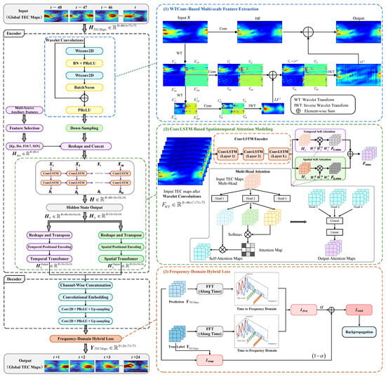
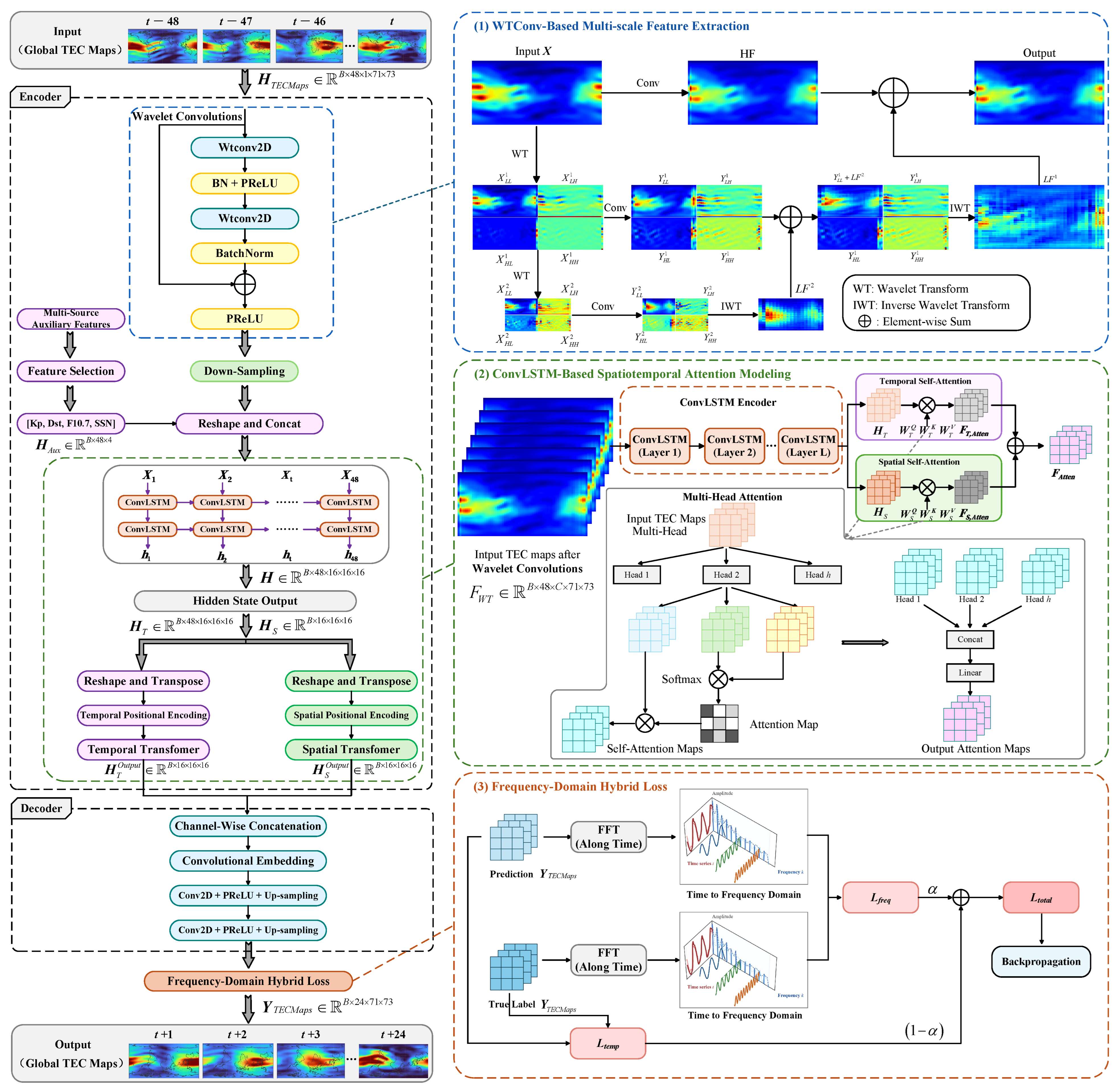
The overall architecture of the proposed DFL-WT-STANet model is illustrated in Figure 1. The framework consists of four main stages: multi-scale feature extraction, spatiotemporal sequence modeling, decoupled spatial–temporal attention, and frequency-domain optimization. The objective is to effectively capture the complex spatiotemporal evolution of TEC while incorporating external space-weather information.

Figure 1. Overall architecture of the proposed DFL-WT-STANet model.

First, the historical TEC maps and auxiliary space-weather features are concatenated to form the model input. The TEC maps provided by CODE GIM have spatial dimensions of 71 × 73, corresponding to a spatial resolution of 2.5° × 5° (latitude × longitude). Since the auxiliary indices (Kp, Dst, F10.7, and SSN) are global scalar values at each observation epoch rather than spatially distributed variables, each index is broadcast into a homogeneous matrix with the same 71 × 73 dimensions as the TEC maps. It ensures dimensional consistency across the input channels while preserving the global nature of the auxiliary indices. Although the spatially replicated auxiliary features do not provide additional spatial variations, they supply global solar and geomagnetic activity information that complements the spatial features extracted from TEC maps. The resulting multi-channel input sequence is then used as input to the spatiotemporal module.

To enhance the representation of multi-scale ionospheric structures, WTConv is employed as the first stage of the network. Through wavelet decomposition, the input TEC maps are separated into low-frequency and high-frequency components, enabling the model to simultaneously capture large-scale background variations and local disturbance features. The extracted multi-scale features are subsequently passed to a ConvLSTM module for spatiotemporal sequence modeling.

After ConvLSTM processing, a decoupled spatial–temporal attention mechanism is introduced. Unlike conventional spatiotemporal attention approaches that jointly model spatial and temporal dependencies, the proposed architecture employs two parallel branches to independently capture global spatial correlations and long-term temporal dependencies. This design reduces feature coupling and improves the efficiency of spatiotemporal representation learning.

Finally, the outputs of the two attention branches are fused and reconstructed through convolutional layers to generate future TEC maps. During training, a frequency-domain hybrid loss is employed to jointly constrain prediction errors in both the time and frequency domains. It helps preserve periodic structures and disturbance characteristics in TEC sequences, thereby improving long-horizon forecasting performance. The detailed implementations of WTConv, the decoupled spatiotemporal attention module, and the frequency-domain hybrid loss are described in the following sections.

2.4. WTConv-Based Multi-Scale Feature Extraction

Global TEC maps contain both large-scale background variations and localized disturbance structures. The large-scale components are mainly associated with long-term solar activity, seasonal variations, and global ionospheric morphology, whereas localized disturbances are often induced by geomagnetic storms, traveling ionospheric disturbances, and other space-weather events. These characteristics result in pronounced multi-scale spatial patterns within TEC data. Conventional CNNs typically rely on stacked local convolution kernels to enlarge the receptive field. However, capturing long-range spatial dependencies often requires deeper network structures, leading to increased computational complexity and potential information loss. Therefore, a Wavelet Transform Convolution (WTConv) module is introduced as the first stage of DFL-WT-STANet. It combines wavelet decomposition and convolutional operations to achieve efficient multi-scale feature extraction. By decomposing the input TEC map into multiple frequency subbands, the model can separately characterize low-frequency background variations and high-frequency disturbance information. Given an input feature map ($\mathbf{X}$), the two-dimensional Haar wavelet transform is first applied to decompose the feature map into four frequency subbands:

$$WT\left(\mathbf{X}\right)=\left\{{\mathbf{X}}_{LL},{\mathbf{X}}_{LH},{\mathbf{X}}_{HL},{\mathbf{X}}_{HH}\right\},$$

(6)

where ${\mathbf{X}}_{LL}$ denotes the low-frequency approximation component, which captures the large-scale background variations of TEC. The ${\mathbf{X}}_{LH}$ and ${\mathbf{X}}_{HL}$ components represent directional high-frequency details associated with spatial variations along the two spatial dimensions, while ${\mathbf{X}}_{HH}$ captures high-frequency details in both dimensions, primarily reflecting diagonal spatial variations. Then, depth-wise convolution is independently applied to each subband:

$${\mathbf{F}}_i=Con{v}_i\left({\mathbf{X}}_i\right),i\in \{LL,LH,HL,HH\},$$

(7)

where $Con{v}_i(·)$ denotes the depth-wise convolution operation on the corresponding frequency subband. Since the convolution is performed in the wavelet domain, WTConv can effectively enlarge the receptive field while maintaining a relatively small number of parameters.

The processed subbands are subsequently reconstructed through the inverse wavelet transform:

$$\mathbf{F}=IWT\left({\mathbf{F}}_{LL},{\mathbf{F}}_{LH},{\mathbf{F}}_{HL},{\mathbf{F}}_{HH}\right),$$

(8)

where $IWT(·)$ denotes the inverse wavelet transform and $\mathbf{F}$ represents the reconstructed feature map.

2.5. ConvLSTM-Based Spatiotemporal Attention Modeling

After WTConv-based feature extraction, the obtained multi-scale feature sequence is combined with auxiliary space-weather information and fed into the translator module for spatiotemporal dependency modeling. The translator consists of two components: a ConvLSTM network for local spatiotemporal feature learning and a dual-path attention mechanism for capturing global spatial and temporal dependencies.

The auxiliary space-weather features, including Dst, Kp, F10.7, and SSN, are expanded into spatial tensors with the same spatial dimensions as the TEC feature maps. These auxiliary tensors are then concatenated with the WTConv feature maps along the channel dimension:

$${\mathbf{F}}_t^{\prime }=Concat({\mathbf{F}}_t,{\mathbf{A}}_t),$$

(9)

where ${\mathbf{F}}_t$ denotes the WTConv feature map at time step t, ${\mathbf{A}}_t$ represents the auxiliary feature tensor, and $Concat(·)$ denotes channel-wise concatenation.

The fused feature sequence is subsequently fed into ConvLSTM to model local spatiotemporal evolution patterns. For each time step, the hidden state and memory state are updated as

$$({\mathbf{H}}_t,{\mathbf{C}}_t)=\mathrm{ConvLSTM}\left({\mathbf{F}}_t^{\prime },{\mathbf{H}}_{t-1},{\mathbf{C}}_{t-1}\right)$$

(10)

where ${\mathbf{H}}_t$ and ${\mathbf{C}}_t$ denote the hidden state and cell state, respectively.

Considering that the recurrent structure of ConvLSTM limits the modeling of long-range temporal correlations, a temporal Transformer branch is introduced to learn long-range dependencies along the temporal dimension: The fused feature sequence is first processed by two stacked ConvLSTM layers to capture local spatiotemporal dependencies. The hidden state sequence generated by the ConvLSTM module can be expressed as:

$$\mathbf{H}=\left\{{\mathbf{H}}_1,{\mathbf{H}}_2,\dots ,{\mathbf{H}}_T\right\},$$

(11)

where ${\mathbf{H}}_t\in {\mathbb{R}}^{H\times W\times C}$ denotes the hidden feature map generated by ConvLSTM at time step t; H and W correspond to the latitude and longitude dimensions of the global TEC map, respectively; and C denotes the number of feature channels. Consequently, the complete hidden-state sequence can be represented as:

$$\mathbf{H}\in {\mathbb{R}}^{T\times H\times W\times C},$$

(12)

where T denotes the temporal length of the input sequence. In this study, $T=48$, $H=71$, $W=73$, and $C=16$ corresponds to the hidden dimension of the ConvLSTM layers.

For temporal attention, the hidden-state tensor is rearranged into temporal token sequences and encoded with temporal positional embeddings for each spatial location. Temporal positional encoding is then added to preserve sequential order information:

$${\mathbf{Z}}_t=Transforme{r}_t\left(P{E}_t\left(\mathbf{H}\right)\right),$$

(13)

where $P{E}_t(·)$ denotes temporal positional encoding and $Transforme{r}_t(·)$ represents the temporal Transformer encoder. The resulting feature representation ${\mathbf{Z}}_t$ captures long-range temporal dependencies and periodic ionospheric variations that cannot be fully modeled by recurrent structures alone.

Similarly, to capture global spatial interactions, the hidden-state tensor is rearranged along the spatial dimension while preserving temporal information. Spatial positional encoding is incorporated to retain geographical location information, and the resulting features are processed by a spatial Transformer encoder:

$${\mathbf{Z}}_s=Transforme{r}_s\left(P{E}_s\left(\mathbf{H}\right)\right),$$

(14)

where $P{E}_s(·)$ denotes spatial positional encoding and $Transforme{r}_s(·)$ represents the spatial Transformer encoder. Through self-attention, the model can establish direct interactions among geographically distant TEC grids, thereby capturing large-scale ionospheric coupling effects.

The outputs of the temporal and spatial Transformer branches contain complementary information regarding long-range temporal evolution and global spatial interactions. To jointly exploit these representations, the resulting feature maps are first reshaped to their original spatiotemporal structure and concatenated along the channel dimension:

$$\mathbf{Z}=\mathrm{Concat}\left({\mathbf{Z}}_t,{\mathbf{Z}}_s\right),$$

(15)

where $\mathrm{Concat}(·)$ denotes channel-wise concatenation.

The fused features are subsequently projected through a convolutional embedding layer and input to the CNN decoder for feature reconstruction. The decoder consists of multiple convolutional and upsampling layers, which progressively recover the spatial resolution and generate the future TEC maps. Through the integration of ConvLSTM and the dual-path Transformer architecture, the proposed translator simultaneously captures local spatiotemporal dynamics, global spatial dependencies, and long-range temporal correlations, thereby providing a comprehensive feature representation for TEC forecasting.

2.6. Frequency-Domain Hybrid Loss

Most existing TEC forecasting models are optimized using time-domain loss functions, such as Mean Squared Error (MSE), which minimize the point-wise discrepancy between predictions and observations. The corresponding time-domain loss is defined over the predicted and observed TEC tensors as

$$L_{temp}={\displaystyle \sum _{i=1}^{T_p}}{∥{\widehat{\mathbf{Y}}}_i-{\mathbf{Y}}_i∥}_2^2$$

(16)

where ${\widehat{\mathbf{Y}}}_i,{\mathbf{Y}}_i\in {\mathbb{R}}^{H\times W}$ denote the predicted and observed TEC maps at the i-th forecast time step, respectively. $T_p$ is the prediction horizon, and H and W correspond to the latitude and longitude dimensions of the global TEC maps, respectively. In this study, $T_p=24$, $H=71$, and $W=73$. The subscript 2 denotes the L2 (Euclidean) norm, and the superscript 2 indicates the squared norm.

Although time-domain losses effectively reduce local prediction errors, they implicitly assume that future labels are independent of each other. TEC evolution exhibits strong temporal autocorrelation due to the combined influence of solar activity, geomagnetic disturbances, and ionospheric dynamical processes. Consequently, adjacent prediction steps are highly correlated. Optimizing only point-wise errors may therefore fail to preserve the intrinsic temporal structure of TEC sequences, particularly in long-horizon forecasting scenarios. Moreover, direct forecasting methods avoid error propagation but usually ignore the dependency structure among future labels. Therefore, how to model the temporal correlation of future TEC sequences while maintaining stable multi-step prediction performance remains a critical challenge.

To address this issue, a frequency-domain learning strategy is introduced. By transforming the prediction sequence from the time domain into the frequency domain, the temporal dependencies among future TEC labels can be represented through different frequency components. This provides an alternative perspective for capturing periodic variations and disturbance-related characteristics in TEC sequences, with the frequency-domain loss given as

$$L_{\mathrm{freq}}={\displaystyle \frac{1}{N_f}}{\displaystyle \sum _{i=1}^{N_f}}{∥{\mathcal{F}}_t{\left(\widehat{\mathbf{Y}}\right)}_i-{\mathcal{F}}_t{\left(\mathbf{Y}\right)}_i∥}_1$$

(17)

where ${\mathcal{F}}_t(·)$ denotes the real-valued discrete Fourier transform along the temporal dimension and $N_f$ represents the number of frequency components. The subscript i denotes the corresponding frequency component. The L1 norm ${\parallel ·\parallel }_1$ represents the mean modulus of the complex-valued spectral differences over the batch and spatial dimensions, where the modulus of a complex number measures its magnitude.

Unlike magnitude-based spectral losses, the proposed formulation directly measures the complex-valued differences between the predicted and observed frequency components. Each complex Fourier coefficient contains both amplitude and phase information. Therefore, the resulting spectral loss is sensitive to discrepancies in both aspects. In particular, phase differences associated with temporal shifts in ionospheric variations contribute to the loss, allowing temporal misalignments in important TEC features, such as the morning rise, diurnal peaks, and storm-related disturbances, to be penalized during optimization. Moreover, the amplitudes of different spectral components may differ by several orders of magnitude. Therefore, the mean absolute complex-valued spectral difference is adopted to evaluate discrepancies across frequency components, providing a direct measure of their combined amplitude and phase differences. Finally, the time-domain and frequency-domain objectives are formulated into a weighted loss function to provide a flexible optimization framework:

$$L_{total}=(1-\alpha )L_{tmp}+\alpha L_{freq}$$

(18)

where $\alpha \in [0,1]$ is a weighting coefficient that controls the relative contributions of the time-domain and frequency-domain loss terms. Different values of $\alpha$ correspond to different optimization configurations, allowing the loss function to be adapted to specific datasets and forecasting tasks.

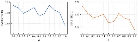
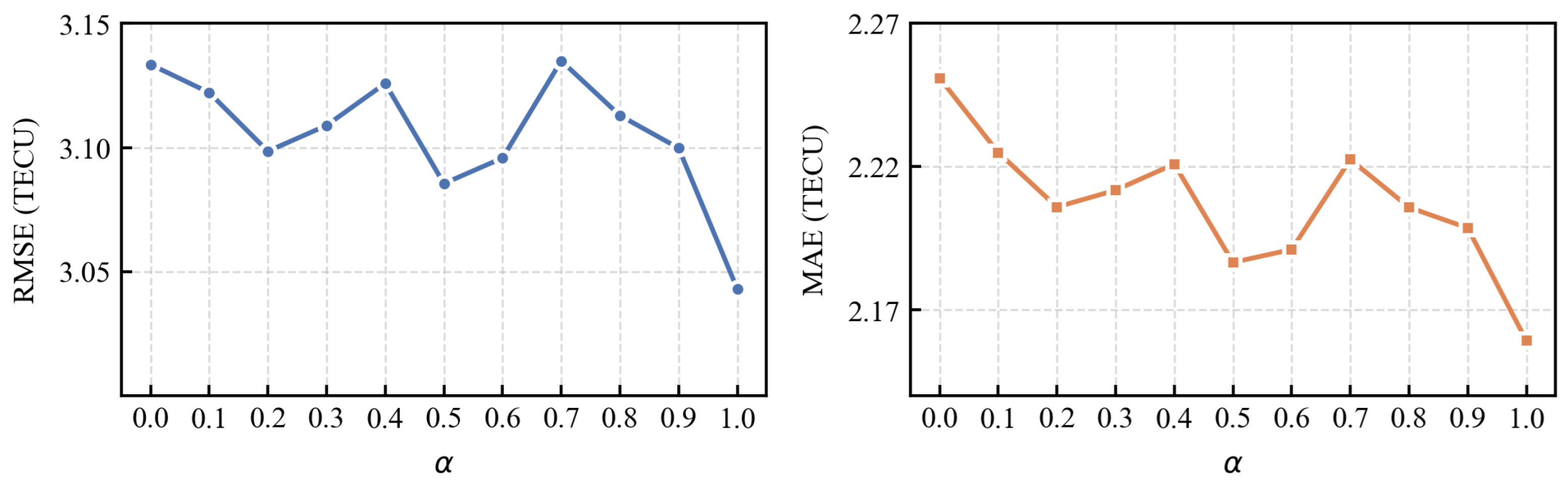
To further investigate the influence of the weighting coefficient ($\alpha$) on forecasting performance, a sensitivity analysis was conducted using the 2015 dataset. The coefficient was varied from 0.0 to 1.0 with an interval of 0.1. For computational efficiency, all sensitivity experiments were conducted using the AdamW optimizer with a learning rate of 0.0005, a batch size of 16, and 15 training epochs. The subsequent main experiments were performed using 100 training epochs.

As shown in Figure 2, the forecasting performance varies with different values of $\alpha$. The lowest RMSE and MAE values of 3.0431 TECU and 2.1593 TECU, respectively, are obtained at $\alpha =1.0$. Compared with the time-domain-only configuration ($\alpha =0.0$), these values are reduced by 2.88% and 4.07%, respectively. Therefore, $\alpha =1.0$ is selected for the subsequent experiments based on its performance under the evaluated dataset and experimental settings. With this setting, the optimization objective reduces to the complex-valued frequency-domain loss. Consequently, the model directly minimizes the discrepancies between the predicted and observed Fourier coefficients, accounting for both amplitude and phase differences across frequency components. This formulation enables the model to capture spectral variations while penalizing temporal shifts in the predicted TEC sequences, thereby improving the representation of periodic patterns and disturbance-related characteristics during multi-step forecasting.

Figure 2. Sensitivity analysis of the weighting coefficient ($\alpha$) in terms of RMSE and MAE on the 2015 dataset.

The output of the decoder corresponds to the future TEC sequence. As defined in Equations (4) and (5) in Section 2.2, the proposed model takes the TEC maps and corresponding auxiliary space-weather indices from the preceding 48 h as input and generates the TEC distribution for the subsequent 24 h, without using any information beyond the current time (t). Specifically, each prediction step produces a global TEC map with a spatial resolution of $71\times 73$, and the complete output sequence consists of 24 consecutive TEC maps. Through the integration of WTConv-based multi-scale feature extraction, ConvLSTM spatiotemporal modeling, dual-path Transformer learning, and frequency-domain optimization, the proposed DFL-WT-STANet effectively captures both local and global spatiotemporal dependencies, thereby improving long-horizon TEC forecasting performance.

2.7. Evaluation Metrics and Hyper-Parameter Settings

To comprehensively evaluate the TEC forecasting performance of different models, two widely used metrics, i.e., the Root Mean Square Error (RMSE) and Mean Absolute Error (MAE), were adopted. Since TEC forecasting involves both long-term temporal evolution and global spatial distribution reconstruction, the evaluation metrics should reflect not only the overall prediction accuracy but also the model’s capability to capture spatial structures and temporal variations.

RMSE is sensitive to large prediction errors and is commonly used to assess the overall deviation between predicted and observed TEC values. MAE provides a more intuitive measure of the average prediction error and is less affected by extreme values. These metrics are defined as follows:

$$RMSE=\sqrt{{\displaystyle \frac{1}{N}}\sum _{i=1}^N{({\widehat{Y}}_i-Y_i)}^2}$$

(19)

$$MAE={\displaystyle \frac{1}{N}}{\displaystyle \sum _{i=1}^N}\left|{\widehat{Y}}_i-Y_i\right|$$

(20)

where ${\widehat{Y}}_i$ and $Y_i$ denote the predicted and observed TEC values, respectively; $\overline{Y}$ represents the mean value of observations; and N is the total number of evaluation samples. Lower RMSE and MAE values indicate better forecasting accuracy. All metrics were calculated using all grid points and forecast horizons of the global TEC maps, thereby providing a comprehensive assessment of model performance under different solar activity conditions.

The network architecture and training hyper-parameters of the proposed DFL-WT-TSANet are summarized in Table 2, including the configurations of the main network components and the settings used during model training.

Table 2. Network architecture and training hyper-parameter settings of DFL-WT-TSANet.

Layer Type and Hyper-Parameters	Settings
WTConv2d	filters = 1, kernel_size = 5, wt_levels = 2
AdaptiveAvgPool2d	output_size = (16, 16)
ConvLSTM	input_dim = 5, hidden_dim = 16, kernel_size = (3, 3), num_layers = 2
Spatial Transformer	embed_dim = 16, num_heads = 4, dropout = 0.2
Temporal Transformer	embed_dim = 16, num_heads = 4, dropout = 0.2
Conv2d (Fusion)	in_channels = 32, out_channels = 16, kernel_size = 1
Decoder Conv2d	hidden_size = 128, activation = PReLU
Upsample	size = (71, 73), mode = bilinear
Conv2d	filters = 24, kernel_size = 3, padding = 1
Optimizer	AdamW
Learning rate	0.0005
Batch size	16
Training epochs	100

3. Results

The forecasting performance of the proposed DFL-WT-STANet is evaluated under different solar and geomagnetic activity conditions. The analysis includes auxiliary feature selection, comparison with representative forecasting models, performance during geomagnetic disturbances, and temporal and latitudinal variations in forecasting accuracy.

3.1. Effect of Solar and Geomagnetic Indices on TEC Forecasting

The ionosphere is jointly influenced by solar radiation and geomagnetic activity. Therefore, selecting appropriate auxiliary space-weather parameters is crucial for improving TEC forecasting performance. To determine the most effective feature combination, a series of comparative experiments were conducted using the WT-ConvLSTM model. The year 2015, corresponding to the maximum phase of Solar Cycle 24, was selected as the test period because ionospheric variability is more pronounced under active solar conditions. Table 3 summarizes the forecasting performance obtained using different combinations of auxiliary space-weather parameters.

Table 3. Comparison of forecasting performance under different auxiliary feature combinations during the solar maximum year 2015.

Auxiliary Features	RMSE (TECU)	MAE (TECU)
F10.7, SSN	3.1495	2.2549
Kp, Ap, Dst	3.1253	2.2402
Kp, Ap, Dst, AE	3.1351	2.2494
Kp, Dst, F10.7, SSN	3.1191	2.2342
Kp, Ap, Dst, F10.7, SSN	3.1195	2.2381
Kp, Ap, AE, Dst, F10.7, SSN	3.1325	2.2497

Note: Bold values indicate the best performance among the compared auxiliary feature combinations.

As shown in Table 3, different combinations of solar and geomagnetic activity indicators were evaluated to identify the most effective auxiliary features for TEC forecasting. Among all tested combinations, the feature set consisting of Kp, Dst, F10.7, and SSN achieved the best performance, with the lowest RMSE and MAE values of 3.1191 TECU and 2.2342 TECU, respectively. Although Ap and AE were included in some candidate combinations, their inclusion did not further improve forecasting performance. In particular, Ap is derived from Kp and provides related geomagnetic activity information, potentially introducing redundant features.

The results demonstrate that solar and geomagnetic activity indicators provide complementary information for TEC prediction. Specifically, F10.7 is closely related to solar extreme ultraviolet radiation and reflects ionospheric ionization intensity, while SSN characterizes long-term variations associated with the solar cycle. In contrast, Kp and Dst describe geomagnetic disturbances and magnetic storm activity, which affect ionospheric electron density redistribution. The combination of these four parameters therefore captures both solar forcing and geomagnetic perturbations, providing complementary physical information for TEC forecasting. Accordingly, Kp, Dst, F10.7, and SSN were selected as the auxiliary features for all subsequent experiments.

3.2. Comparative Evaluation of Different Prediction Models

To evaluate the effectiveness of the proposed model, five TEC forecasting approaches were compared: CODE’s 1 day-predicted product (C1PG), Encoder–Decoder ConvLSTM (ED-ConvLSTM), Wavelet Transform ConvLSTM (WT-ConvLSTM), Wavelet-based Spatiotemporal Attention Network (WT-STANet), and the proposed Dual-domain Filtered-label Wavelet-based Spatiotemporal Attention Network (DFL-WT-STANet). The experiments were conducted for 2015, 2019, and 2024, representing different levels of solar activity. The forecasting performance of the five models is summarized in Table 4.

Table 4. Forecasting performance of different models under different solar activity conditions.

Year	Model	RMSE (TECU)	MAE (TECU)
2015	C1PG	4.0468	2.8264
	ED-ConvLSTM	3.2940	2.3920
	WT-ConvLSTM	3.1191	2.2342
	WT-STANet	3.0424	2.1859
	DFL-WT-STANet	2.9643	2.1017
2019	C1PG	1.4780	1.0170
	ED-ConvLSTM	1.2448	0.9229
	WT-ConvLSTM	1.2273	0.8880
	WT-STANet	1.1820	0.8642
	DFL-WT-STANet	1.1520	0.8262
2024	C1PG	6.4445	4.5796
	ED-ConvLSTM	5.2701	3.8319
	WT-ConvLSTM	5.1885	3.7346
	WT-STANet	4.8522	3.4762
	DFL-WT-STANet	4.8144	3.4298

Note: Bold values indicate the best performance among the compared methods.

As shown in Table 4, DFL-WT-STANet consistently achieves the lowest RMSE and MAE among all five models across the three test years. In 2015, the proposed model achieves an RMSE of 2.9643 TECU and an MAE of 2.1017 TECU. Compared with C1PG, these values correspond to reductions of 26.75% and 25.64%, respectively. A similar advantage is observed in 2024, when the overall forecasting errors are substantially higher because of the stronger TEC variability. DFL-WT-STANet still obtains the lowest RMSE and MAE of 4.8144 and 3.4298 TECU, representing reductions of 25.29% and 25.11%, respectively, compared with C1PG. These results demonstrate that the proposed model maintains a clear forecasting advantage during periods of elevated solar activity.

Compared with the deep-learning-based models, a progressive reduction in both RMSE and MAE can also be observed from ED-ConvLSTM to WT-ConvLSTM and further to WT-STANet, indicating the benefits of multi-scale wavelet feature extraction and spatiotemporal attention modeling. More importantly, DFL-WT-STANet further improves upon WT-STANet in all three test years. In 2015, RMSE decreases from 3.0424 to 2.9643 TECU and MAE from 2.1859 to 2.1017 TECU, corresponding to reductions of 2.57% and 3.85%, respectively. In the relatively quiet year of 2019, DFL-WT-STANet achieves an RMSE of 1.1520 TECU and an MAE of 0.8262 TECU, further reducing the errors by 2.54% and 4.40% relative to WT-STANet. Even in 2024, when the prediction task becomes more challenging, the proposed model retains the best performance, with RMSE and MAE reductions of 0.78% and 1.33%, respectively, over WT-STANet.

In addition to forecasting accuracy, the computational complexity and inference efficiency of the proposed model were evaluated on an NVIDIA RTX 2080 Ti GPU. ED-ConvLSTM, WT-ConvLSTM, WT-STANet, and DFL-WT-STANet were compared in terms of total parameters, trainable parameters, inference time per TEC map, and peak GPU memory usage. As shown in Table 5, DFL-WT-STANet contains 89,232 parameters, including 89,168 trainable parameters, identical to WT-STANet. In terms of inference efficiency, DFL-WT-STANet requires 21.88 ms per TEC map, compared with 22.14 ms for WT-STANet, while the peak GPU memory usage increases slightly from 0.168 GB to 0.176 GB. These results indicate that the frequency-domain optimization introduces no additional network parameters and only a marginal increase in memory consumption, without increasing inference time. Considering its consistent forecasting improvements across the three test years, the proposed model achieves additional predictive benefits with comparable computational complexity and inference efficiency.

Table 5. Computational complexity and inference efficiency of different models on an NVIDIA RTX 2080 Ti GPU.

Model	Parameters	Trainable Parameters	Inference Time (ms/map)	Peak GPU Memory (GB)
ED-ConvLSTM	82,098	82,098	17.78	0.198
WT-ConvLSTM	77,428	77,364	20.24	0.087
WT-STANet	89,232	89,168	22.14	0.168
DFL-WT-STANet	89,232	89,168	21.88	0.176

Note: Bold values indicate the proposed DFL-WT-STANet model and its corresponding complexity metrics.

Overall, the results demonstrate that DFL-WT-STANet provides consistent improvements under both active and quiet solar conditions. The substantial error reductions relative to C1PG demonstrate the overall forecasting advantage of the proposed deep-learning framework, while the further improvements over WT-STANet indicate the effectiveness of the complex-valued frequency-domain optimization in enhancing TEC forecasting accuracy. Furthermore, the computational complexity analysis shows that these improvements are achieved without increasing the network parameter count or introducing substantial inference overhead. These findings demonstrate the effectiveness and computational efficiency of the proposed model for global TEC forecasting under different solar activity conditions.

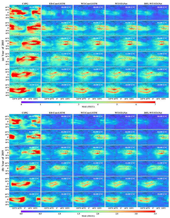
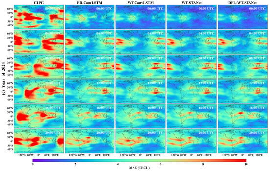
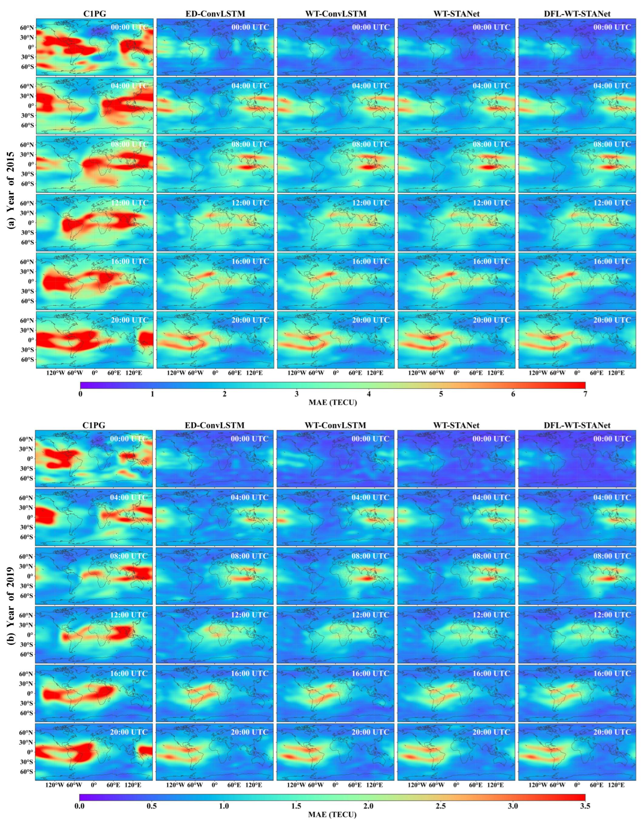
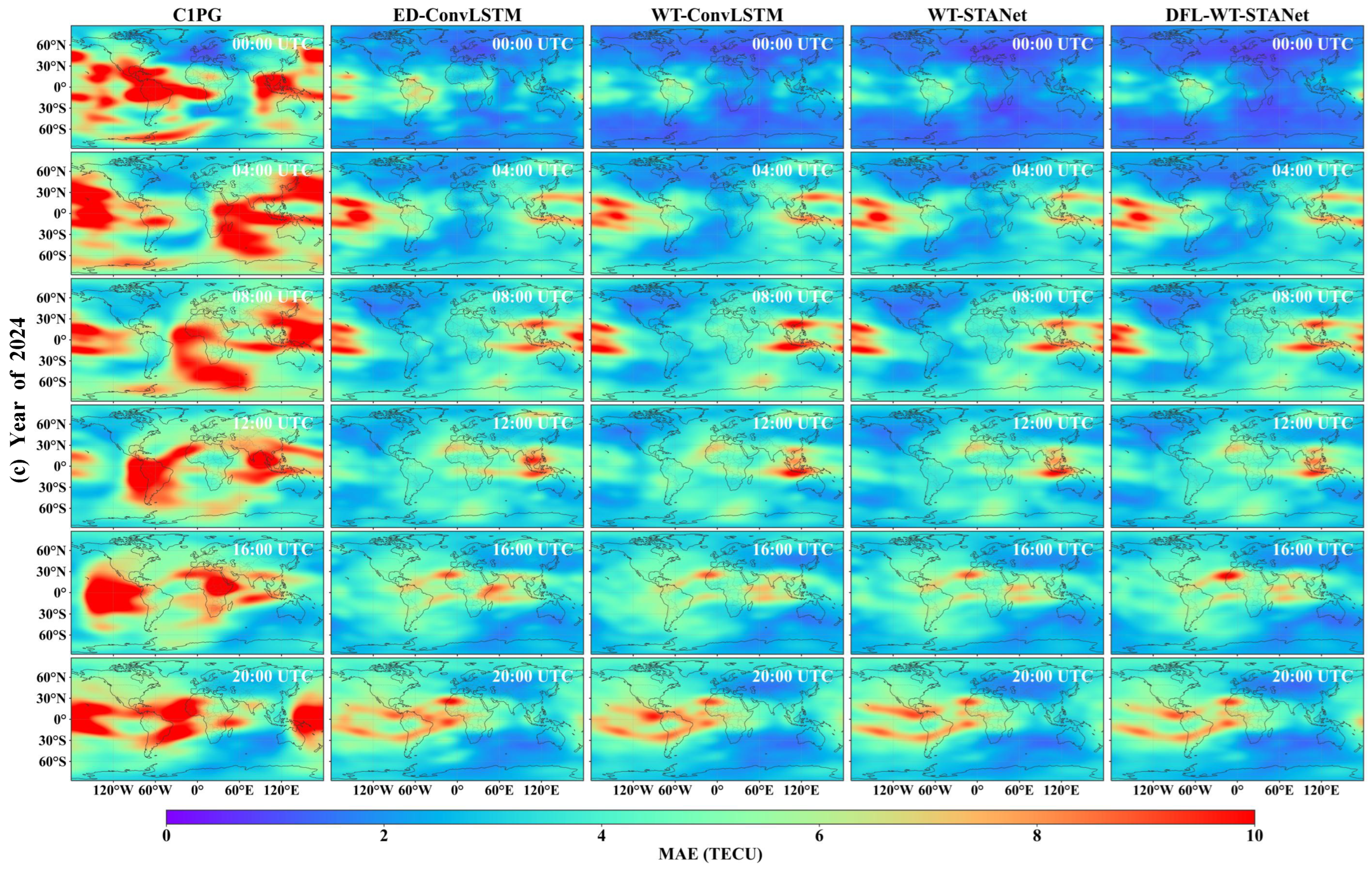
To further investigate the spatial distribution of forecasting errors, Figure 3 presents the annual mean absolute errors of the global TEC prediction maps at six representative UTC times for (a) 2015, (b) 2019, and (c) 2024. These spatial error distributions provide a more detailed evaluation of the forecasting performance of different models under different solar activity conditions.

Figure 3. Annual MAEs of global TEC prediction maps at 00:00, 04:00, 08:00, 12:00, 16:00, and 20:00 UTC for (a) 2015, (b) 2019, and (c) 2024. Columns from left to right correspond to C1PG, ED-ConvLSTM, WT-ConvLSTM, WT-STANet, and DFL-WT-STANet.

As shown in Figure 3a, the prediction errors in 2015 exhibit pronounced spatial and temporal variations. C1PG shows relatively large errors over extensive areas, particularly at low and equatorial latitudes, where TEC variations are generally more pronounced. In comparison, the deep-learning-based models substantially reduce both the error magnitude and the spatial extent of large errors. With the progressive introduction of wavelet-based multi-scale feature extraction and spatiotemporal attention mechanisms, the spatial prediction errors are further reduced. In particular, WT-STANet and DFL-WT-STANet exhibit lower prediction errors at most of the selected UTC times, with notable improvements in the equatorial and low-latitude ionosphere.

Similar spatial characteristics can also be observed in Figure 3b,c. The overall error magnitude is considerably lower in 2019, whereas larger and more widespread prediction errors occur in 2024, indicating the increased difficulty of TEC forecasting under enhanced solar activity. Despite the substantial differences in error magnitude among the three years, WT-STANet and DFL-WT-STANet consistently exhibit smaller spatial prediction errors than the other models. This advantage is particularly evident in the TEC error distributions at 04:00 and 20:00 UTC in 2024. Together with the quantitative results reported in Table 4, these spatial comparisons demonstrate the effectiveness of WT-STANet in predicting regional TEC variations and the further improvement achieved by DFL-WT-STANet under different solar activity conditions. Furthermore, during representative geomagnetic storm events, DFL-WT-STANet exhibits better forecasting performance than WT-STANet, which will be analyzed in detail in the following subsection.

3.3. Geomagnetic Storm Events for TEC Predicting Evaluation

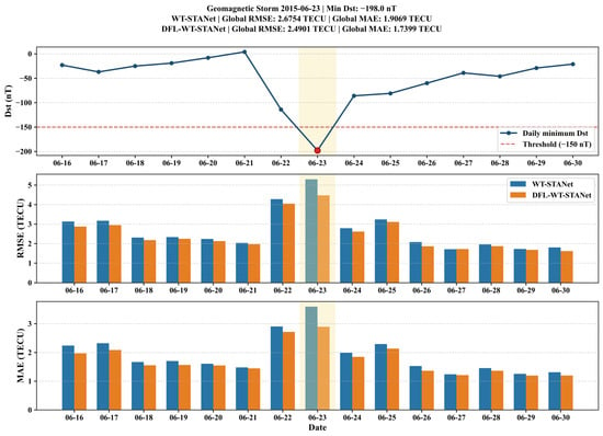
To further evaluate the forecasting performance of the proposed model under different geomagnetic activity conditions, four representative periods were selected for detailed analysis, as summarized in Table 6. The selected periods cover different levels of geomagnetic activity, with minimum Dst values ranging from $-55$ to $-406$ nT. Period 1 (16–30 June 2015) corresponds to a strong geomagnetic storm, whereas Period 2 (25 August–8 September 2019) represents relatively quiet geomagnetic conditions. Periods 3 (4–18 May 2024) and 4 (4–18 October 2024) experienced much stronger geomagnetic disturbances, with minimum Dst values of $-406$ and $-333$ nT, and are classified as severe geomagnetic storm events. These four periods provide representative cases for assessing the robustness of TEC prediction models under different levels of geomagnetic disturbance.

Table 6. Selected geomagnetic storm events for TEC forecasting evaluation.

Geomagnetic Storm Event	Minimum Dst (nT)	Storm Level
Period 1: 16–30 June 2015	$-198$	Strong
Period 2: 25 August–8 September 2019	$-55$	Quiet
Period 3: 4–18 May 2024	$-406$	Severe
Period 4: 4–18 October 2024	$-333$	Severe

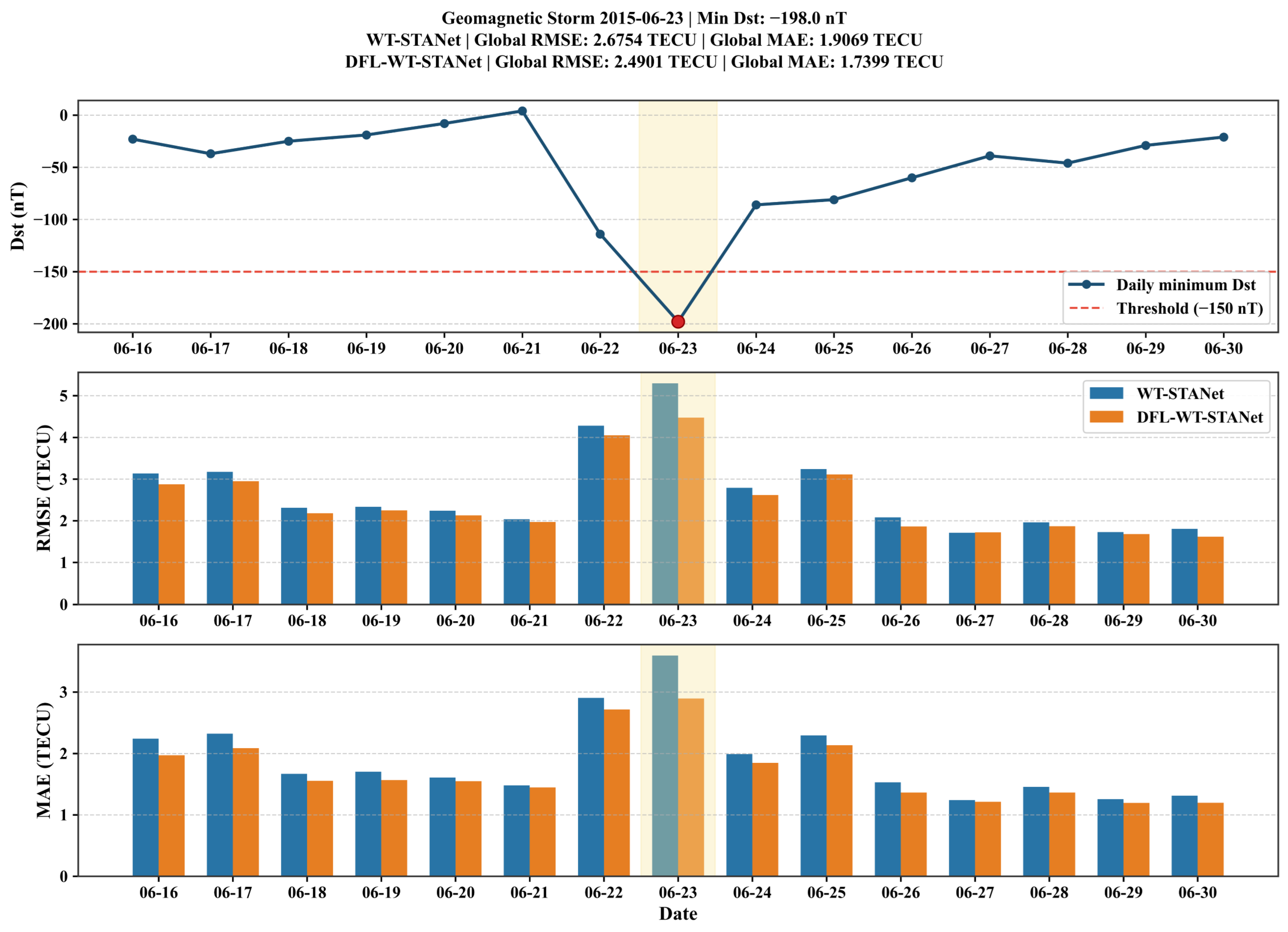
Among the baseline models evaluated in Section 3.2, WT-STANet exhibits the strongest overall forecasting performance. Therefore, WT-STANet was selected as the primary reference model for a more detailed comparison with DFL-WT-STANet under geomagnetically disturbed conditions. Period 1 was used as a representative case to examine the temporal evolution of forecasting errors during a geomagnetic storm. Figure 4 presents the variation in Dst over the 15-day analysis window together with the daily mean RMSE and MAE of WT-STANet and DFL-WT-STANet. The forecasting errors exhibit clear temporal variations during this period, with increased errors around the geomagnetically disturbed interval. Nevertheless, DFL-WT-STANet generally maintains lower daily RMSE and MAE than WT-STANet, indicating more stable forecasting performance during the evolution of this storm event.

Figure 4. Temporal variations in Dst and daily mean TEC forecasting errors of WT-STANet and DFL-WT-STANet during Period 1. The yellow shaded region indicates the geomagnetic storm day.

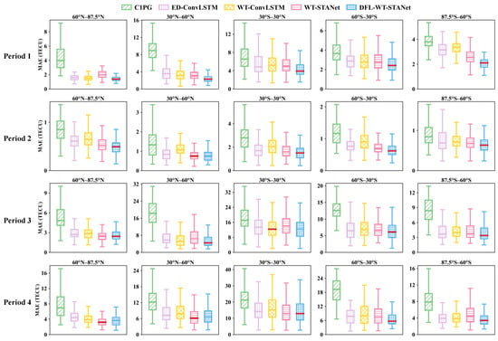
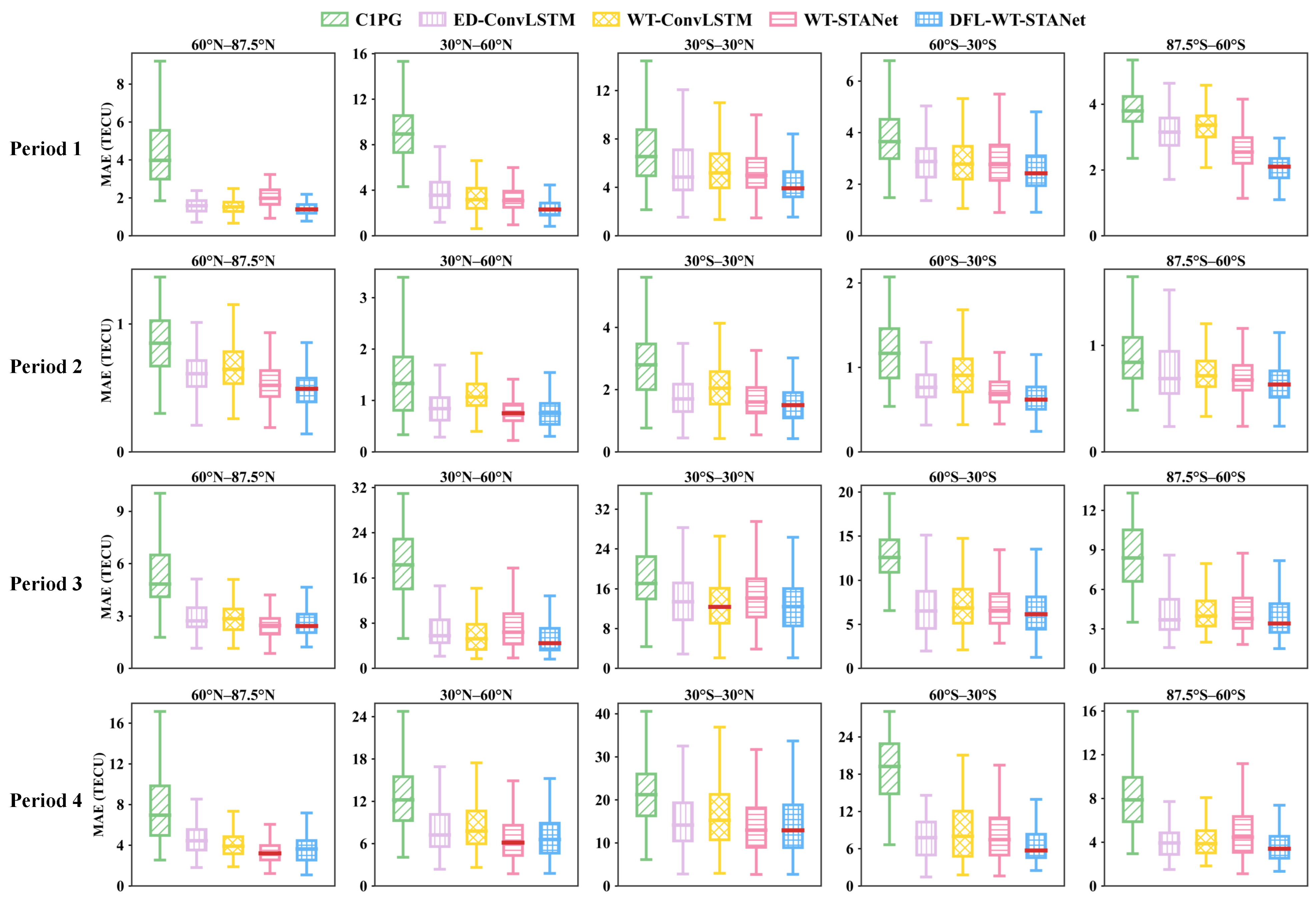
While the above case study provides a detailed temporal comparison between DFL-WT-STANet and the strongest baseline, a broader evaluation involving all five models is required to assess whether the forecasting advantage is maintained across different geomagnetic activity conditions and latitude regions. Therefore, the analysis was further extended to the four selected periods and five latitude bands. Considering the strong latitudinal dependence of ionospheric TEC, the global grid points were divided into five latitude bands: ${60}^{\circ }$ N–$87.5^{\circ }$ N, ${30}^{\circ }$ N–${60}^{\circ }$ N, ${30}^{\circ }$ N–${30}^{\circ }$ S, ${30}^{\circ }$ S–${60}^{\circ }$ S, and ${60}^{\circ }$ S–$87.5^{\circ }$ S. Figure 5 compares the MAE distributions of the five models across these latitude bands for the four selected periods.

Figure 5. MAE distributions of different TEC prediction models across five latitude bands during four representative geomagnetic activity periods. The red line represents the minimum median value across the compared models.

As shown in Figure 5, DFL-WT-STANet generally achieves the lowest median MAE across the different latitude bands for all four periods, indicating that its forecasting advantage is maintained under different levels of geomagnetic activity. In addition to the median MAE, the boxplot distributions show that DFL-WT-STANet also performs favorably in terms of the interquartile and overall error ranges. This advantage is particularly evident across all five latitude bands in Period 1. Similar improvements can be observed in the ${60}^{\circ }$ N–$87.5^{\circ }$ N, ${30}^{\circ }$ N–${60}^{\circ }$ N, and ${30}^{\circ }$ N–${30}^{\circ }$ S bands during Period 2; the ${30}^{\circ }$ N–${60}^{\circ }$ N and ${60}^{\circ }$ S–$87.5^{\circ }$ S bands during Period 3; and the ${30}^{\circ }$ S–${60}^{\circ }$ S and ${60}^{\circ }$ S–$87.5^{\circ }$ S bands during Period 4.

Overall, the results demonstrate that DFL-WT-STANet maintains consistently low forecasting errors across different latitude bands, even as the geomagnetic activity varies substantially among the four selected periods. The improvements in both the median MAE and the overall error distributions further indicate the robustness of the proposed model for global TEC forecasting under geomagnetically disturbed conditions.

In addition to the latitudinal error distributions, Table 7 provides a quantitative comparison between WT-STANet and DFL-WT-STANet during three representative geomagnetic storm events. Both the mean RMSE and MAE over each 15-day analysis window and the corresponding errors on the storm day are reported. Overall, DFL-WT-STANet achieves lower errors for most metrics, with its advantage becoming more evident under enhanced geomagnetic disturbances.

Table 7. Comparison of WT-STANet and DFL-WT-STANet during representative geomagnetic storm events.

Period	Min Dst (nT)	Model	15-Day Mean (TECU)		Storm Day (TECU)
			RMSE	MAE	RMSE	MAE
Period 1 16–30 June 2015	$-198$	WT-STANet	2.6754	1.9069	7.3206	5.0475
		DFL-WT-STANet	2.4901	1.7399	7.3066	4.9807
Period 3 4–18 May 2024	$-406$	WT-STANet	6.1819	4.2514	12.3113	8.4088
		DFL-WT-STANet	6.1496	4.1779	11.2120	7.4568
Period 4 4–18 October 2024	$-333$	WT-STANet	7.8578	5.6086	13.1335	8.9077
		DFL-WT-STANet	7.9182	5.6044	12.8281	8.5512

Note: Bold values indicate the better performance between WT-STANet and DFL-WT-STANet for each metric.

For Period 1, DFL-WT-STANet reduces the 15-day mean RMSE and MAE by 6.93% and 8.76%, respectively, compared with WT-STANet, indicating an overall improvement throughout the analysis window. During the severe geomagnetic storm in Period 3, the advantage becomes particularly pronounced on the storm day, with RMSE and MAE reductions of 8.93% and 11.32%, respectively. For Period 4, the corresponding storm-day reductions are 2.33% and 4.00%. Although WT-STANet achieves a slightly lower 15-day mean RMSE in Period 4, DFL-WT-STANet still performs better in both RMSE and MAE on the storm day.

These results indicate that DFL-WT-STANet maintains competitive performance over the complete 15-day periods while providing a clearer advantage during geomagnetic storm days. Together with the latitude-dependent error distributions shown in Figure 5, the results demonstrate the robustness of DFL-WT-STANet across different latitude bands and geomagnetic activity levels, particularly during periods of pronounced ionospheric disturbance.

3.4. Temporal and Latitudinal Consistency of TEC Forecasting Performance

Although the preceding experiments demonstrate the overall forecasting advantage of DFL-WT-STANet, annual evaluation metrics alone cannot fully characterize whether this advantage is consistently maintained over different time periods and spatial regions. Therefore, the forecasting performance of the five models was further evaluated from monthly and latitudinal perspectives.

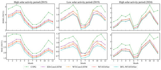
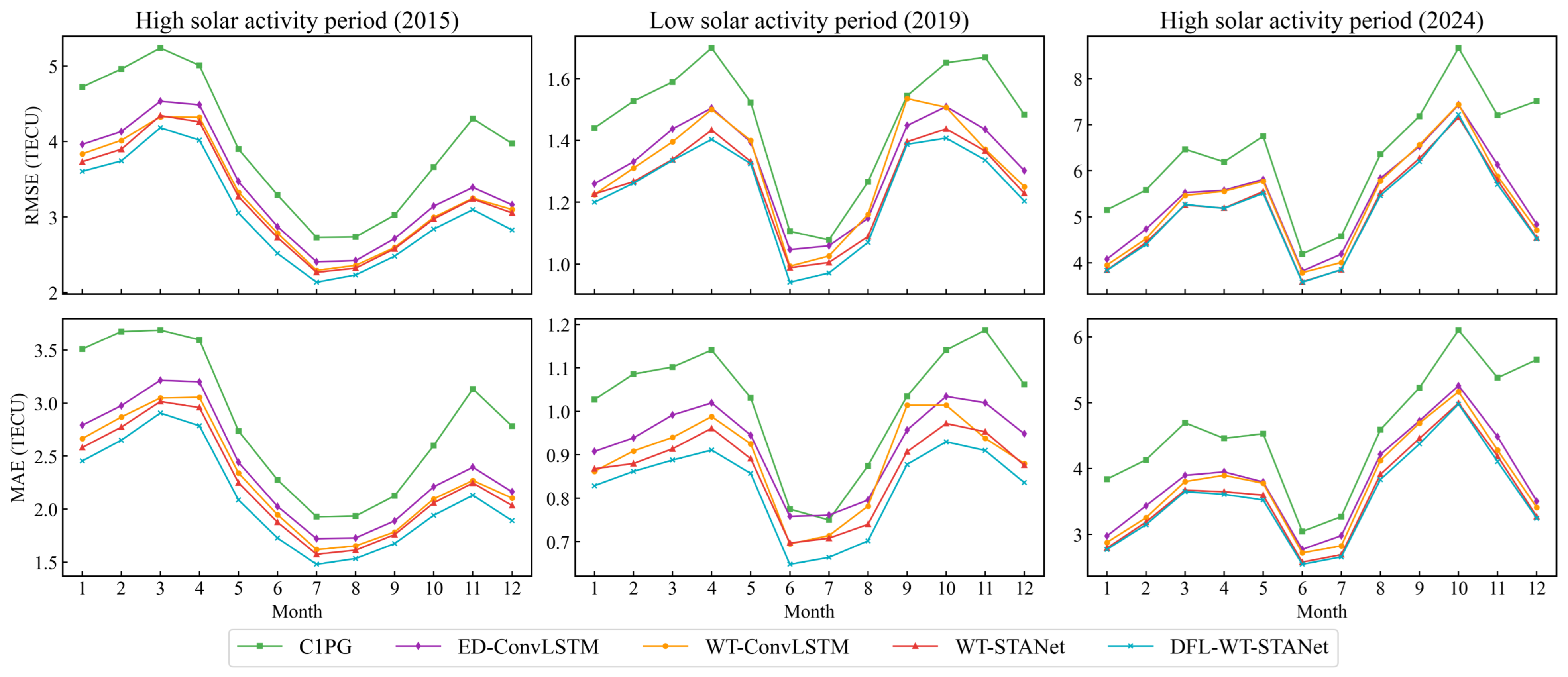
Figure 6 presents the monthly mean RMSE and MAE of the five models for 2015, 2019, and 2024. Specifically, a 24-h sliding step was adopted to construct consecutive daily forecasting samples. The TEC maps and auxiliary features from the preceding 48 h were used to predict the subsequent 24-h TEC sequence. For each daily prediction, RMSE and MAE were calculated over the 24 forecast time steps and all 71 × 73 global grid points. The monthly metrics were then obtained by averaging the corresponding daily RMSE and MAE values over all forecasting days within each month. The forecasting errors exhibit clear month-to-month variations, and their overall magnitudes differ substantially among the three years. In particular, the errors are generally lower in 2019, whereas larger fluctuations and higher error levels are observed in 2015 and 2024. Despite these temporal variations, DFL-WT-STANet generally maintains lower RMSE and MAE than the other models across most months. This result indicates that the forecasting advantage of the proposed model is not confined to a specific period but remains consistent across different months and solar activity conditions.

Figure 6. Monthly RMSE and MAE of different TEC forecasting models averaged over the corresponding daily values.

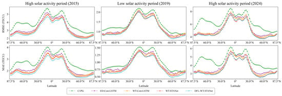
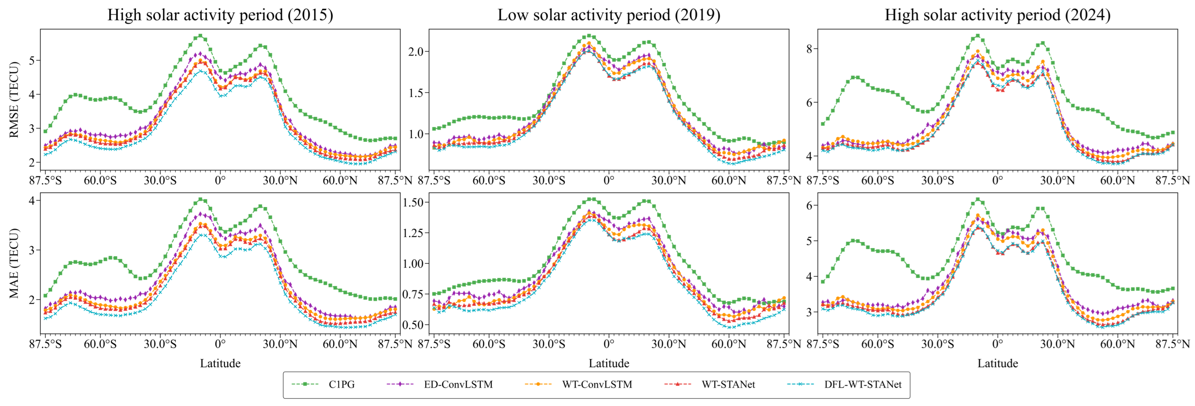
In addition to the temporal consistency, the forecasting performance was further examined along the latitudinal direction. The global TEC grid contains 71 latitude points with a spatial interval of $2.5^{\circ }$. For each latitude, the RMSE and MAE were calculated by aggregating the prediction errors across all evaluated forecasting days, the 24 forecast time steps, and the corresponding 73 longitude grid points. This procedure yielded a latitude-dependent error profile for each model, reflecting its forecasting accuracy across different latitudinal regions. Figure 7 presents the resulting RMSE and MAE variations with latitude for the five forecasting models.

Figure 7. Latitude-dependent RMSE and MAE of different TEC forecasting models averaged over the corresponding longitude grid points.

The error distributions show a clear dependence on latitude, reflecting the spatial heterogeneity of global TEC variations. Although the error magnitude varies considerably across latitude regions, DFL-WT-STANet generally exhibits lower RMSE and MAE than the other models over most latitudes. More importantly, its advantage is maintained across a broad range of latitude regions rather than being concentrated within a specific spatial region. These results indicate that the proposed model provides more consistent forecasting performance across the global ionospheric grid.

Overall, the monthly and latitude-dependent evaluations provide complementary evidence for the temporal and spatial consistency of DFL-WT-STANet. Combined with the annual comparisons and geomagnetic storm analyses presented in the preceding subsections, these results demonstrate that the forecasting advantage of the proposed model is maintained across different temporal scales, latitude regions, and geomagnetic activity conditions.

4. Conclusions

This study proposed DFL-WT-STANet for global ionospheric TEC forecasting, aiming to improve the modeling of complex spatiotemporal variations in TEC. The proposed framework integrates wavelet-based multi-scale feature extraction, spatiotemporal attention modeling, and a dual-domain optimization strategy that jointly constrains prediction errors in the time and frequency domains. In addition, Kp, Dst, F10.7, and SSN were incorporated as auxiliary space-weather parameters to provide information on solar and geomagnetic activity. Using the previous 48 h observations as input, the model predicts global TEC maps for the subsequent 24 h.

Experiments were conducted using global TEC data covering different solar activity conditions, with 2015, 2019, and 2024 selected as representative test years. DFL-WT-STANet consistently achieved the lowest RMSE and MAE among the five evaluated forecasting approaches. Compared with C1PG, the RMSE was reduced by 26.75%, 22.06%, and 25.29% in 2015, 2019, and 2024, respectively. Further evaluations under representative geomagnetic storm events showed that the proposed model maintained its forecasting advantage under disturbed ionospheric conditions. In particular, during the severe geomagnetic storm in Period 3, the storm-day RMSE and MAE were reduced by 8.93% and 11.32%, respectively, compared with WT-STANet. The monthly and latitude-dependent evaluations further demonstrated that this advantage was maintained across different months and a broad range of latitude regions, indicating consistent temporal and spatial forecasting performance.

Overall, the results demonstrate that DFL-WT-STANet provides accurate and robust global TEC forecasts under different solar and geomagnetic activity conditions, with particular advantages during periods of pronounced ionospheric disturbance. Nevertheless, the present study mainly evaluates forecasting performance using historical global TEC maps and space-weather indices. Future work will investigate the model under a wider range of extreme space-weather events and explore the incorporation of additional physical information to further improve the forecasting of rapid and localized ionospheric variations.

References

- Aguiar, C.R.; Monico, J.F.G.; Moraes, A.O. Impact of ionospheric scintillations on GNSS availability and precise positioning. Space Weather 2025, 23, e2024SW004217. [Google Scholar] [CrossRef] [Scilit]
- Zhbankov, G.A.; Danilkin, N.P.; Maltseva, O.A. Influence of the ionosphere on the accuracy of the satellite navigation system. Acta Astronaut. 2022, 190, 194–201. [Google Scholar] [CrossRef] [Scilit]
- Zhao, X.; Lu, X.; Quan, W.; Li, X.; Zhao, H.; Lin, G. An effective ionospheric TEC predicting approach using EEMD-PE-Kmeans and self-attention LSTM. Neural Process. Lett. 2023, 55, 9225–9245. [Google Scholar] [CrossRef] [Scilit]
- Bilitza, D.; Altadill, D.; Truhlik, V.; Shubin, V.; Galkin, I.; Reinisch, B.; Huang, X. International Reference Ionosphere 2016: From ionospheric climate to real-time weather predictions. Space Weather 2017, 15, 418–429. [Google Scholar] [CrossRef] [Scilit]
- Wang, N.; Yuan, Y.; Li, Z.; Li, Y.; Huo, X.; Li, M. An examination of the Galileo NeQuick model: Comparison with GPS and JASON TEC. GPS Solut. 2017, 21, 605–615. [Google Scholar] [CrossRef] [Scilit]
- Li, Q.; Yang, D.; Fang, H. Two hours ahead prediction of the TEC over China using a deep learning method. Universe 2022, 8, 405. [Google Scholar] [CrossRef] [Scilit]
- Liu, Y.; Yang, K.; Sun, L.; Wang, J.; Smirnov, A.; Xiong, C. Modeling and prediction of the ionosphere with deep learning: A review. Intell. Robot. 2026, 6, 67–95. [Google Scholar] [CrossRef] [Scilit]
- Zhang, R.; Li, H.; Shen, Y.; Yang, J.; Li, W.; Zhao, D.; Hu, A. Deep learning applications in ionospheric modeling: Progress, challenges, and opportunities. Remote Sens. 2025, 17, 124. [Google Scholar] [CrossRef] [Scilit]
- Tang, J.; Ding, M.; Yang, D.; Fan, C.; Khonsari, N.; Mao, W. Different data-driven prediction of global ionospheric TEC using deep learning methods. Int. J. Appl. Earth Obs. Geoinf. 2024, 130, 103889. [Google Scholar] [CrossRef] [Scilit]
- Ruwali, A.; Kumar, A.J.S.; Prakash, K.B.; Sivavaraprasad, G.; Ratnam, D.V. Implementation of hybrid deep learning model (LSTM-CNN) for ionospheric TEC forecasting using GPS data. IEEE Geosci. Remote Sens. Lett. 2020, 18, 1004–1008. [Google Scholar] [CrossRef] [Scilit]
- Ren, X.; Zhao, B.; Ren, Z.; Wang, Y.; Xiong, B. Deep Learning-Based Prediction of global ionospheric TEC during storm periods: Mixed CNN-BiLSTM method. Space Weather 2024, 22, e2024SW003877. [Google Scholar] [CrossRef] [Scilit]
- Liu, W.; Luo, Z.; Wei, N.; Deng, Z.; Yao, Z. ED-ST-Transformer: A global TEC spatiotemporal prediction model based on multisource data. Space Weather 2025, 23, e2025SW004484. [Google Scholar] [CrossRef] [Scilit]
- Liu, Y.; Gong, Y.; Zhang, H.; Hu, Z.; Yang, G.; Yuan, H. A new and tested ionospheric TEC prediction method based on SegED-ConvLSTM. Remote Sens. 2025, 17, 885. [Google Scholar] [CrossRef] [Scilit]
- Yang, J.; Huang, W.; Zhang, L.; Xu, H.; Shen, H.; Wang, X.; Li, M. Ionospheric TEC forecasting with ED-ConvLSTM-Res integrating multi-channel features. Remote Sens. 2025, 17, 3564. [Google Scholar] [CrossRef] [Scilit]
- Gao, X.; Yao, Y. A storm-time ionospheric TEC model with multichannel features by the spatiotemporal ConvLSTM network. J. Geod. 2023, 97, 9. [Google Scholar] [CrossRef] [Scilit]
- De Paulo, M.C.M.; Marques, H.A.; Feitosa, R.Q.; Ferreira, M.P. New encoder–decoder convolutional LSTM neural network architectures for next-day global ionosphere maps forecast. GPS Solut. 2023, 27, 95. [Google Scholar] [CrossRef] [Scilit]
- Lin, M.; Zhu, X.; Tu, G.; Chen, X. Optimal Transformer modeling by space embedding for ionospheric total electron content prediction. IEEE Trans. Instrum. Meas. 2022, 71, 8505414. [Google Scholar] [CrossRef] [Scilit]
- Li, S.; Liu, H.; Le, H.; Sun, L.; Yao, X. Ionospheric TEC spatiotemporal prediction based on MFEM-ConvLSTM. Adv. Space Res. 2026, 78, 6410–6428. [Google Scholar] [CrossRef] [Scilit]
- Xue, K.; Shi, C.; Wang, C. RA-ConvLSTM: Recurrent-architecture attentional ConvLSTM networks for prediction of global total electron content. Space Weather 2025, 23, e2024SW004173. [Google Scholar] [CrossRef] [Scilit]
- Ma, Y.; Yuan, J.; Liu, H.; Zhang, Z.; Zhou, R.; Xiao, J.; Yuan, G. CGConvLSTM: A spatial-aware ionospheric total electron content spatiotemporal prediction model. Space Weather 2025, 23, e2025SW004528. [Google Scholar] [CrossRef] [Scilit]
- Fathy, A.; Farid, A.I.S.; Okoh, D.; Mungufeni, P.; Mahrous, A.; Nassar, M.; Otsuka, Y.; Fu, W.; Habarulema, J.B.; El-Husseiny, H.; et al. U-Net based forecasting of storm-time total electron content over North Africa using assimilation of GNSS observation into global ionospheric maps. Universe 2026, 12, 54. [Google Scholar] [CrossRef] [Scilit]
- Lin, M.; Ma, H.; Zhu, X.; Tu, G.; Li, A.; Pan, H. TEC prediction using cross-attention spatiotemporal feature weighted BiConvLSTM and improved pre-earthquake anomaly detection. Space Weather 2026, 24, e2025SW004787. [Google Scholar] [CrossRef] [Scilit]
- Li, D.; Jin, Y.; Wu, F.; Zhao, J.; Min, P.; Luo, X. A hybrid model for TEC prediction using BiLSTM and PSO-LSSVM. Adv. Space Res. 2024, 74, 303–318. [Google Scholar] [CrossRef] [Scilit]
- Zhou, S.; Shi, Z.; Fu, H. Prediction of global ionospheric TEC based on deep learning and singular spectrum analysis. In Proceedings of the 2023 International Applied Computational Electromagnetics Society Symposium (ACES-China), Hangzhou, China, 15–18 August 2023; pp. 1–3. [Google Scholar] [CrossRef] [Scilit]
- Nath, S.; Chetia, B.; Kalita, S. Ionospheric TEC prediction using hybrid method based on ensemble empirical mode decomposition (EEMD) and long short-term memory (LSTM) deep learning model over India. Adv. Space Res. 2023, 71, 2307–2317. [Google Scholar] [CrossRef] [Scilit]
- Bhardwaj, S.; Chandrasekhar, E.; Padiyar, P.; Gadre, V.M. A comparative study of wavelet-based ANN and classical techniques for geophysical time-series forecasting. Comput. Geosci. 2020, 138, 104461. [Google Scholar] [CrossRef] [Scilit]
- Zhou, R.; Liu, H.; Le, H.; Xiao, J.; Ma, Y.; Yuan, J.; Shan, W.; Wang, M. CSA-WTConvLSTM: A TEC spatiotemporal prediction model focusing on both low-frequency and high-frequency features. Space Weather 2025, 23, e2025SW004338. [Google Scholar] [CrossRef] [Scilit]
- Zhao, J.; Wang, Q.; Wu, F.; Jiang, H.; Li, D. FVMD-HTLD: Prediction of TEC based on signal decomposition and integrated models. Adv. Space Res. 2026, 77, 3404–3417. [Google Scholar] [CrossRef] [Scilit]
- Li, A.; Zhu, X.; Lin, M.; Tu, G.; Yan, Z. Ionospheric TEC prediction using the non-stationary inverted transformer fusion model and its performance in Chinese region. GPS Solut. 2025, 29, 204. [Google Scholar] [CrossRef] [Scilit]
Disclaimer/Publisher’s Note: The statements, opinions and data contained in all publications are solely those of the individual author(s) and contributor(s) and not of MDPI and/or the editor(s). MDPI and/or the editor(s) disclaim responsibility for any injury to people or property resulting from any ideas, methods, instructions or products referred to in the content. |
© 2026 by the authors. Licensee MDPI, Basel, Switzerland. This article is an open access article distributed under the terms and conditions of the Creative Commons Attribution (CC BY) license.