


Abstract
Bosonic particles beyond the Standard Model, such as axions, are among the leading candidates for dark matter. If such particles have a small mass, they are usually described as a purely classical field. However, it was recently shown that this description is incomplete: their inherent gravitational self-interactions result in the squeezing of the field, which is a quantum characteristic that is beyond the classical description. Here we analyze squeezing of light dark matter in the presence of decoherence. We show that squeezing is continuously generated rapidly enough to survive dissipation, and it may also remain present under thermal fluctuations and dephasing. Our results demonstrate that dark matter might possess persistent quantum features and motivate further investigation of their implications for dark matter detection.
1. Introduction
Axions and axion-like particles constitute one of the most motivated extensions of the Standard Model of particle physics and are among the leading candidates for dark matter [1,2,3]. Originally introduced in connection to the strong CP problem [4,5,6], axions have since become a much broader phenomenological framework that includes ultralight axion particles [7,8], string-inspired models and the axiverse [9,10] and coherent bosonic dark matter spanning many orders of magnitude in mass [11,12,13].
Even though their coupling to ordinary matter and photons is extremely weak [14], they do provide the portals through which axions and axion-like particles can be searched for [15,16,17,18,19,20,21,22,23]. At the same time, their gravitational and cosmological effects provide complementary probes [24,25,26,27,28,29]. This has motivated large experimental and observational efforts ranging from axion haloscopes [30] and helioscopes [31,32,33] to precision interferometry [34,35,36], astrophysical probes [37,38] and cosmological structure formation [7,8,12].
For the purposes of this work, the most important aspect of axion dark matter is that it is usually treated as a highly occupied bosonic field [12,39,40]. For a representative QCD-axion mass, and , the occupation number in a de Broglie volume can be enormous, of order , for typical galactic dark matter velocities [39]. In the ultralight mass regime, , the occupation number becomes even larger, potentially reaching , while the de Broglie wavelength reaches galactic scales – [39,41,42,43]. This highly occupied wave-like regime motivates the common description of axion dark matter as a coherently oscillating classical field, an assumption that underlies many recent proposals for ultralight dark matter detection [44,45,46,47,48,49].
However, the classical description of the field may not be sufficient [50,51,52,53,54] even though it is deeply rooted in the standard treatment of ultralight axion dark matter. In the usual argument, the axion field is highly occupied, , and therefore the size of the initial relative quantum fluctuations under the coherent state assumption is expected to scale as . The dynamics is then assumed to be captured by mean-field classical equations of motion, such as the Gross–Pitaevskii or Schrödinger–Newton equations [40,55,56,57]. This viewpoint provides the basis for much of the axion phenomenology. However, a large occupation number by itself does not provide a sufficient criterion for classicality. In quantum optics and quantum information science, classicality or non-classicality is a property of the quantum state and not only its mean occupation number, and quantum features can take many different forms. For instance, non-classicality is usually benchmarked through criteria such as the non-positivity of the Glauber–Sudarshan P-function, presence of quadrature squeezing, sub-Poissonian statistics, Wigner negativity and entanglement, among many others [58,59,60,61,62,63,64,65]. For axions, large occupation only says that the initial fluctuations may be small. If the Hamiltonian that drives the dynamics is nonlinear, as is the case for self-gravitating and self-interacting axions [1,66], these fluctuations can evolve non-trivially even when the mean field itself continues to obey a classical equation of motion. This is familiar from quantum optics and cold atoms physics such as in Bose–Einstein condensates, which is often the analogy to ultralight fields, where highly occupied fields evolving under nonlinear dynamics give rise to squeezing and other non-classical signatures despite the fact that their mean field satisfies a classical equation of motion [67,68,69,70].
In a previous work [52], we showed that non-classical features in fact do arise naturally in ultralight axion-like fields, where squeezing is generated on short timescales: keeping the quantum operator associated with the highly occupied axion mode while imposing the Hartree/mean-field ansatz for the mode functions, the quantum operator obeys a nonlinear Kerr-oscillator equation of motion [71,72]. At the level of the mean field, the evolution appears to be classical. However, at the level of the fluctuations, the nonlinear evolution squeezes the quantum state. As a result, an initial coherent state does not remain coherent under the evolution: the quadrature fluctuations rapidly fall below the coherent/vacuum noise level from just the inherent gravitational dynamics of the field. In this sense, axion dark matter can develop a genuinely quantum feature even in a regime that is usually regarded as classical. An analogue of this effect is well-known in Bose–Einstein condensates [69,70,73], which may seem to behave as a classical wave but in fact represent a deeply quantum mechanical phenomenon exhibiting quantum features. For ultralight axions, in addition to inherent squeezing from the nonlinear evolution demonstrated in our work [52], other non-classical features have recently been proposed [74,75].
Here, we investigate whether the rapid squeezing of axions can survive under decoherence. The single-mode unitary analysis in [52] establishes that gravitational self-interactions lead to squeezing. Here, we study its robustness against a range of different decoherence mechanisms that are likely to arise. This is especially important because decoherence is often invoked as the mechanism that restores classical behavior [76,77,78,79,80]. If the environmental interactions destroy the squeezing on a shorter timescale than its onset, no observational consequences would be expected. On the other hand, if squeezing is re-generated before decoherence becomes dominant or, similarly, if the quadrature noise remains below the vacuum plateau for a finite window of time, then quantum dynamics of axions may survive and have observable consequences. Here we show that squeezing may indeed remain robust against decoherence. We study a broad range of decoherence mechanisms, such as multi-mode interactions in the field, dissipation and dephasing into both the vacuum and a thermal bath. Our results show that the inherent nonlinearity of the field evolution can be stronger than the decoherence, and squeezing of axions may survive in the real world.
The paper is organized as follows. In Section 2, we summarize our previous findings on axion squeezing in [52] for the unitary single-mode axion dynamics. We then proceed to analyze its robustness against decoherence through an open-system analysis. In Section 3, we introduce a two-mode axion toy model, illustrating the inter-mode couplings that appear to generate entanglement, and show how tracing over one mode yields reduced-state dephasing. We highlight that the squeezing survives and is very robust in such a model. In Section 4, we study the effect of representative Markovian environments on Kerr squeezing, focusing on zero-temperature damping, dephasing and finite-temperature dissipation. We derive the corresponding expressions for the minimal quadrature variance and identify the regimes in which squeezing survives. Finally, we summarize our conclusions in Section 5 and present supporting derivations in the Appendix A and Appendix B.
2. Summary of Unitary Axion Dynamics
In this section, we summarize our core results in [52]. In a nutshell, Ref. [52] showed that axion-like dark matter, although it is usually described as a classical field [8,12,39,40], naturally develops a genuinely quantum mechanical feature through its gravitational interaction: quadrature squeezing below the coherent-state or vacuum level. The standard argument for treating axions as a classical field is based on their enormous occupation number [40]. In the late universe, many axions occupy the same macroscopic field configuration, and the relative size of quantum fluctuations is expected to scale as [40]. This motivates the usual Gross–Pitaevskii [81] or Schrödinger–Poisson description, where the axion field is effectively treated as a classical wave [39].
The main message of [52] is that this classical-field intuition (or description) is incomplete. If one keeps the quantum operator associated with the macroscopically occupied mode, , the same gravitational self-interaction that appears in the Gross–Pitaevskii equation also generates, at the operator level, a Kerr-type quantum nonlinearity [71]. This term, which is intrinsic to the gravitational dynamics of the field, squeezes the quantum fluctuations around the mean field, as we briefly summarize below.
To briefly illustrate our finding, our starting point in [52] is the Hartree approximation in which the non-relativistic axion quantum field is assumed to be dominated by a single mode,
Here is normalized such that and obeys the usual mean-field Schrödinger–Poisson dynamics, while remains a genuine annihilation operator satisfying . The naive classical approximation corresponds to replacing
This replacement gives the standard classical field description but discards the quantum fluctuations/noise of the axion field. The key observation of our work [52] is that this discarded quantum noise is not passive but dynamically squeezed by the self-gravity of the axion field.
The dynamics of the operator takes the form of a well-studied model in quantum optics and cold atoms, the so-called Kerr oscillator [68,69,70,71,72,82,83,84,85,86]
which is generated by a nonlinear Hamiltonian of the form1
where is the strength of the nonlinearity2. The nonlinear Kerr term makes different number components of the quantum state rotate slightly differently. As a result of this, in phase space, an initial circular coherent-state uncertainty distribution is ‘twisted’, as illustrated in Figure 1. The effect to lowest order is that one quadrature, which we call minimal variance or principal squeezing [84,87,88,89], becomes narrower than the vacuum level, while its conjugate becomes broader (at later times, the field becomes even more non-classical and the Kerr nonlinearity generates large Schrödinger cat states, but, here, we focus on the most robust quantum effect of squeezing). Defining [67], squeezing occurs when the minimal quadrature variance in the Heisenberg picture satisfies
As an initial state, the axion field is taken to begin in a coherent state . While this might be expected for a classical field, this is not an ad hoc choice. Instead, it is physically motivated by the so-called misalignment mechanism [1,2,3]. In the early universe, the axion field is assumed to be initially displaced from the minimum of its potential. While the Hubble rate is larger than the axion mass , the field is approximately frozen by Hubble friction. Later, when the Hubble rate becomes smaller than the mass, , the field begins to oscillate coherently around the minimum of its potential [12]. Classically, this gives a homogeneous oscillating scalar field. Quantum mechanically, the state that most closely represents a classical field with a well-defined amplitude and phase is a coherent state [58]. Therefore the coherent state is not an arbitrary choice: it is the natural quantum representative of the classical field produced by misalignment. For a coherent state, the relative field fluctuations of the occupied mode scale as [40]
Figure 1.
Evolution of the Wigner function with of an initially coherent state under the Kerr Hamiltonian (4). Here, is the strength of Kerr nonlinearity. The figure shows the early-time nonlinear shearing and quadrature squeezing. At later times, the full unitary Kerr evolution includes interference fringes, cat-like states, and revival [71,85]. Here, we are focusing only on squeezing before the onset of other coherent effects, which, however, is already a signature of quantum behavior.
For a large occupation number that is typical for axions [39], we get . This is the standard classicality argument of axion dark matter. However, as we show in [52], even if the field initially looks classical, the Kerr evolution (3) subsequently unitarily turns this apparently classical state into a squeezed state, as illustrated in Figure 2.
Figure 2.
Squeezing of axion dark matter as found in [52]. The cyan shading represents the Wigner function , with darker shades indicating larger values. In the main panels, orange markers denote the classical solution , while the small dark dots denote the quantum mean . Finally, the orange bars in the bottom panel indicate the annotated phase-space width scalings. An initial coherent state develops quadrature squeezing that results in the reduction in its quantum noise below the vacuum level , reaching at . Maximal squeezing is reached at . The minimal quadrature variance starts at and reaches at . Finally, at , the variance is [52]. The inset illustrates the exact minimal quadrature variance normalized to the vacuum value of one with the three stages/times marked.
Although an initial coherent state is physically motivated in the context of axion dark matter, we should stress that it is not essential for the squeezing mechanism described in Ref. [52]. The crucial aspect in our analysis is that the Kerr evolution operator, around a mean field, can be approximated as an effective squeezing operator (see Appendix C in Ref. [52]). As a result, reduced quadrature fluctuations for a broader class of initial states are possible, including displaced thermal states. However, in that case, going below the vacuum level would need stronger squeezing due to the additional initial noise of the state. In what follows, we focus on an initially coherent state.
Given the inherent nonlinear axion dynamics, squeezing occurs for arbitrarily small positive time t. In [52], we operationally define the squeezing timescale as the time required to reach . This becomes, in the above model,
At first sight, this appears to depend on the number of axions N. However, for the self-gravitating axion mode considered in [52], the Kerr coupling parameter scales as . This is one of the most important conclusions in our previous work: The onset of squeezing is independent of the number of axions N and does not become slower for larger occupation number.3 Large N makes the mean field look classical, but it does not delay the quantum squeezing of the fluctuations around that mean field. For cosmological axion dark matter, we have estimated the squeezing time (see Equation (12) in [52])
The derivation and assumptions underlying this unitary estimate are discussed in detail in Ref. [52], whose Table I summarizes the characteristic squeezing timescales and maximal squeezing for cosmological volumes, solitonic cores and galactic haloes. is the typical axion velocity for virialized cosmological axions in galactic halos [39] and is the reduced de Broglie wavelength. For a QCD axion with a theoretically expected mass the result is of the order of
Thus, squeezing is generated on extremely short timescales compared with cosmological evolution. In particular, as illustrated in Figure 3 for axions in the mass range , including ultralight axion dark matter candidates [8], the squeezing timescale turns out to be cosmologically relevant. Unitary squeezing can grow until it reaches its first maximum at
Figure 3.
Cosmological squeezing timescales as functions of the axion mass-energy. The blue curve shows the onset time , while the orange curve shows the time at which maximal squeezing is reached. The dashed horizontal line denotes the age of the universe. The shaded region marks axion masses , for which the estimated time to reach maximal unitary squeezing exceeds the age of the universe. It is clear that, over the plotted axion mass range, the onset of squeezing is well below the age of the universe.
Here N denotes the occupation of the single Hartree mode over the selected volume V. For the cosmological benchmark of Ref. [52], V was chosen to be of order the present Hubble volume. For axions in a Hubble volume, this yields , corresponding to a remarkable ∼313 dB of squeezing.4 The required time to reach this maximum is
Figure 4 illustrates how this maximum squeezing depends on the axion mass. For QCD-like axions with , the value of is still much shorter than the age of the universe. On the other hand, for sufficiently ultralight axions , the onset of squeezing can still be fast, but the system would not reach the maximal squeezing within the age of the universe.
Figure 4.
Maximum attainable squeezing of the cosmological axion mode as a function of the axion mass-energy. The curve shows the estimate in [52], which is obtained from the large occupation number of axions in a Hubble volume, . For the mass of the QCD axion, , the value of maximum squeezing is . The vertical dotted line indicates the mass for which the time to reach maximal squeezing equals the age of the universe, . For larger masses, , the maximal squeezing is reached within the age of the universe.
Thus, the conclusion is that the intrinsic self-interactions contained in the axion field dynamics generate squeezing on extremely short timescales. It can reach enormous values, but the overall size of the effect depends on the axion mass. Therefore, one might expect that ultralight axion dark matter evolves rapidly into a quantum state and that it could be highly squeezed in the process.
In addition to just the dynamics of the field in a cosmological setting, we have also considered other self-gravitating situations, such as galactic halos and solitonic cores [41], and found the same qualitative result: the onset of squeezing is extremely rapid compared with astrophysical timescales. This result challenges the standard view that the axion field can simply be regarded as a coherent classical field. At the same time, our analysis is not outside the standard axion framework. It is precisely the Hartree approximation that leads to the Kerr oscillator for the occupied mode. In this sense, the squeezing is a quantum effect sitting on top of the usual mean-field description, and its description arises consistently within the same framework. We also note that this exact behavior is also expected in Bose–Einstein condensates [70,97].
However, these results are only valid for a closed-system description in which the field evolves unitarily. Most importantly, the derivation assumes unitary evolution of a simple single-mode axion system, neglecting both environmental decoherence and possible multi-mode effects of the field. It is thus natural to ask whether squeezing may be maintained in a real-world scenario or whether decoherence completely destroys its appearance.
In the following, we go beyond this idealized unitary picture, retaining the Kerr squeezing mechanism while embedding the single axion mode in an open-system setting. In what follows, we will study how the minimal variance evolves under zero-temperature dissipation, finite-temperature dissipation, and pure dephasing. The central question then becomes a competition between the gravitational squeezing scale, controlled by , and the relevant environmental rates. Ultimately, this open-system extension will inform us on how much of the gravitationally generated axion squeezing survives once the ideal single-mode picture is embedded in a more realistic late-universe environment. As we show below, our results suggest that the expected squeezing may be robust even in the presence of interactions with an environment.
3. Two-Mode Axion Dynamics, Entanglement and Reduced State Dephasing
In [52], we considered the axion dark matter field consisting of a single mode. The dynamics were treated within the Hartree approximation, which guarantees the validity of the Gross–Pitaevskii equation while retaining the full quantum operator nature of the field operators. That is, the non-relativistic axion field operator is , keeping intact. This approach led to a system of equations that combines the usual Gross–Pitaevskii dynamics for with a nonlinear Kerr oscillator equation of motion for , which, when acting on an initially coherent state, produces large quadrature squeezing.
Here, we relax the single-mode restriction and consider the case where axion dark matter comprises two interacting modes. This provides an analytically tractable model for examining how the neglected degrees of freedom in the single-mode description affect squeezing. Our motivation is to show that different inter-mode couplings give rise to richer axion dynamics, such as entanglement between modes, and that the standard assumption of classicality may break down even for very simple two-mode models.
In Section 3.1, we present the multi-mode Hamiltonian for non-relativistic gravitationally interacting axions. In Section 3.2 we develop the two-mode truncation and analyze the exactly solvable dynamics, which include cross- and self-Kerr interactions. We compute the reduced density matrix of the selected mode a, the minimal quadrature variance and the linear entropy. Finally, in Section 3.3, we briefly introduce the Markovian Lindblad framework for more general environments, which will prepare the broader analysis in Section 4.
3.1. Multi-Mode Hamiltonian for Non-Relativistic Gravitationally Interacting Axions
We consider a non-relativistic axion field interacting through Newtonian gravity, neglecting non-gravitational self-interactions and external potentials. Throughout this section, we use the frequency Hamiltonian . The corresponding Hamiltonian reads [40,98,99]
The Heisenberg equation of motion for the non-relativistic axion field is5
where
the Newtonian potential, satisfying the Poisson equation . We expand the axion field with respect to a complete orthonormal set of mode functions , that is, , where and [98]. The equation of motion for the annihilation operator is
where the kinetic matrix elements are
and the gravitational self-couplings
The Hamiltonian, in terms of creation and annihilation operators, in full generality, is [98,101]
This mode representation makes explicit the dynamics and interactions of a selected axion mode. The coefficients appearing in the multi-mode Hamiltonian (17) arise from the inherent gravitational interactions and include self-Kerr, cross-Kerr and other processes that redistribute axion particles between modes. Their magnitudes, in the case of a single self-gravitating axion dark matter field without any other external environment, are fixed by the spatial profiles and normalization of the modes. Thus, Hamiltonian (17) lists the interaction processes that are, in principle, allowed by its operator structure but does not imply that every term is non-zero for every choice of modes.
A single orbital/mode function does not, by itself, determine the quantum state of the associated mode: Its quantum fluctuations can evolve non-trivially, as in the case of Kerr dynamics discussed in Section 2 and [52]. Allowing additional occupied modes introduces the possibility of inter-mode interactions. Systematic treatments of such dynamics are well-studied in the context of Bose–Einstein condensates, including multi-configurational6 approaches [102].
3.2. Two-Mode Axion Dynamics
We now restrict the axion field expansion to two orthonormal modes. This truncation provides a more tractable setting in which we can identify how the inter-mode interactions affect the quantum state of a selected mode and therefore its squeezing. Our aim in this subsection is to illustrate the interplay between the self-Kerr squeezing and the coupling to an unobserved mode without attempting a complete description of the multi-mode axion dynamics. In this setting, the non-relativistic axion field operator takes the form
where annihilate an axion in the modes and , respectively. The Hamiltonian in such a case is
where, for notational simplicity, we define and . This Hamiltonian preserves the total axion number; namely, . The corresponding kinetic matrix elements and the gravitational quartic coefficients are given by (15) and (16), respectively.
In Figure 5 we illustrate the physical meaning of each term in the Hamiltonian (19). These processes are well-studied in quantum optics [103]. Hamiltonian (19) and simplified versions of it, as we will see below, is able to capture the quantum seeds of decoherence and the breakdown of classicality of axion dark matter from its multi-mode behavior alone without an external environment. However, we should mention that this Hamiltonian corresponds to a toy model in the sense that it cannot reproduce or describe effects such as the irreversibility and thermalization [50,66] that characterize a realistic many-mode system. In that sense, it is not a fully realistic model of decoherence, but it shows that the inclusion of additional modes can reduce squeezing effects. Our goal here is to illustrate the relative interplay between the generation of squeezing and its loss due to mode interactions before considering a general open-system treatment.
Figure 5.
Physical processes associated with the two-mode axion Hamiltonian in Equation (19). For a detailed discussion of the analogous processes in quantum optics, see Ref. [103].
We focus here on just two modes interacting through the cross-Kerr coupling and compute the reduced dynamics of one mode after tracing out the second, showing how entanglement between the modes as well as the coupling between modes can affect the Kerr-induced squeezing.
3.2.1. Illustrative Example: Particle Conservation Within Each Mode
To illustrate how the inter-mode couplings can affect the squeezing, we focus on a scenario in which no particle exchange occurs between modes a and b. That is, we keep only those terms in (19) that conserve the particle number in each mode separately; namely, . The Hamiltonian then reads
The first two terms describe the usual free evolution, the third and fourth terms describe the self-Kerr evolution for each mode and the last term is a cross-Kerr coupling between modes a and b. For an initial state that is a product of coherent states, , the problem can be analytically solved, leading to the exact time-evolved state
with angular frequency eigenvalues given by
The Fock-basis matrix elements of the density matrix are
Tracing out the b-mode, , we get the reduced density of the a-mode
3.2.2. Computation of the Minimal Variance
Having the exact solution of the reduced density matrix for the mode a, after tracing out the b-mode, we can compute the minimal quadrature variance
for the initial state . A straightforward calculation of the various moments leads to the exact solution at all times,
For , we recover the single-mode Kerr result [88,89]. Moreover, the self-Kerr evolution of the b-mode, namely terms that are proportional to , does not appear in (27), as expected. The reason is that the Hamiltonian of b-mode commutes with the cross-Kerr interaction. Since this part of the system acts only on the traced-out subsystem, it cancels under the partial trace and therefore has no effect on the reduced state of the a-mode.
In order to capture the onset of squeezing at early times, it is sufficient to Taylor expand the minimal variance to get
This equation makes explicit the competition between the different contributions: The linear-in-time self-Kerr term, , drives the variance below the vacuum noise level and is therefore responsible for the onset of squeezing. By contrast, the positive terms increase the variance and therefore counteract the squeezing. The term corresponds to a higher-order correction to the linear-in-time self-Kerr term, which, during the onset of squeezing, tends to drive the minimal variance back to . The environmental correction stemming from tracing out the b-mode is
To gain some intuition, we define the dimensionless parameter
When , that is, when , the mode a behaves almost as the usual single-mode Kerr oscillator. The coupling to the b-mode is not important during the onset of squeezing. On the other hand, when , the state of a-mode still exhibits squeezing (recall that appears linearly in time t) but the amount is reduced compared to the single-mode Kerr case, as can be seen from Figure 6.
Figure 6.
Evolution of the minimal quadrature variance , as given by Equation (27), for two equally occupied modes that are both initially in a coherent state, comparing (blue solid curves) and (red dashed curves). From left to right, the coupling ratio of the cross- to self-Kerr couplings is . Time is expressed through the dimensionless variable R. The main panels use logarithmic axes, while the insets show only the onset of evolution on linear axes. The dashed horizontal line marks the vacuum variance, , below which is an indication of quadrature squeezing. Clearly, squeezing develops initially in all three cases. Increasing the inter-mode coupling reduces the achievable squeezing depth. In a similar spirit as in Appendix B in Ref. [52], using , the magnitude of squeezing is when , when and when . Note that, for larger , for instance in the case of axions in a cosmological Hubble volume [39,52], we get a deeper corresponding to for the leftmost panel, as discussed in Section 2 and Ref. [52]. The middle and right panels instead approach finite variance floors corresponding to approximately and , respectively. The finite squeezing and its eventual loss is due to further unitary evolution that produces other highly non-classical states beyond the squeezing that is depicted in Figure 1, not decoherence.
In other words, as long as , the initial slope of the minimal variance is always negative, meaning that there is always the initial squeezing.
This example highlights a crucial point for our analysis: moving from a single-mode axion model to the two-mode axion model already captures the fact that squeezing is not automatically destroyed by the presence of an additional environmental mode b. The extent to which squeezing becomes substantial depends on the details of the specific model, especially the relative coupling strengths () and the relative number of axions within each mode and .
3.2.3. Linear Entropy and Entanglement Between Modes
Computing the linear entropy , we get
The entropy captures the entanglement generated between the two modes for a bipartite pure state. We can immediately observe that, at initial time , the linear entropy vanishes, , as expected for a product state. On the other hand, at any time , the linear entropy is positive except for the times for , which are the so-called revival times, and holds. A positive linear entropy therefore establishes entanglement between the modes a and b.
This simple calculation illustrates that, under the cross-Kerr coupling, an initial pure product state of coherent states evolves into an entangled two-mode state. Tracing out the b-mode leads to a mixed state for the a-mode, which cannot be described by a single coherent state. For axion dark matter, such couplings are inevitably present even in the absence of any external environment since gravitational self-interactions generate both self-Kerr and cross-Kerr terms together with mode-changing interaction terms, as is clear from Equation (19).
We should keep in mind that the “environment” in the previous example consists only of a single mode (b), and the decoherence is periodic and reversible. At certain times the off-diagonal factor in (24) returns to 1 and the coherence revives completely. In other words, this is not an irreversible Lindblad-type decoherence but simply a unitary dephasing and re-phasing cycle, similar in spirit to the Jaynes–Cummings model in quantum optics [104]. In Section 4, we will discuss the phenomenological approach to axion dark matter decoherence using Markovian Lindblad equations. In particular, we return to the case of dephasing for a generic bath in Section 4.2.
3.3. Transition to a Generic Quantum Open System Analysis: Markovian Master Equation in Lindblad Form
The previous two-mode calculation illustrates how coupling to an unobserved degree of freedom generates entanglement and modifies the squeezing of a selected axion mode. Its role is simply to provide a tractable example of this mechanism. It is only a very specific and analytically controlled microscopic example that is useful because one can explicitly see which operator structures are present in the many-mode axion Hamiltonian. However, a more realistic model may involve additional unresolved axion modes or other environmental degrees of freedom. To investigate the robustness of Kerr squeezing across such settings, in Section 4, we introduce an effective description that captures the relevant environmental processes without requiring a complete microscopic model of axions and each environment separately. The Lindblad framework provides such a description: if the reduced dynamics of the selected system is Markovian, then the generator of completely positive and trace preserving (CPTP) dynamics must have the Gorini–Kossakowski–Sudarshan–Lindblad (GKLS) form [105,106,107]
where denotes the reduced density matrix of the selected system (for instance the a-mode of the axion field), is the system Hamiltonian and is the anti-commutator. Once the operators have been specified, all the remaining influence of the environment is encoded in the rates while the dissipator captures the non-unitary piece of the dynamics [108].
This equation provides a very general description of a selected quantum system interacting with unresolved environmental degrees of freedom in the Markovian limit. Its strength is precisely its generality: this equation captures a very broad class of physical environments whose detailed microscopic origin (their exact Hamiltonian dynamics) may significantly differ and lead to different jump operators but, nevertheless, lead to the same Lindblad structure, Equation (32).
The inter-mode couplings in the axion Hamiltonian provide microscopic motivation for several possible environmental channels. Couplings that exchange particles between the selected mode and unresolved modes motivate loss and gain processes, while occupation-dependent couplings, such as cross-Kerr couplings, motivate phase noise. However, whether these processes admit a Markovian description depends on the dynamics and correlations of the environment.
In Section 4, we study loss, pure dephasing, and finite-temperature damping phenomenologically and determine their effects on the onset, magnitude, and duration of Kerr squeezing. The resulting conditions apply to different physical environments whenever the corresponding effective channel is justified. Application to a particular axion setting requires estimates of the relevant environmental parameters.
4. Effect of Generic Environments on Kerr Squeezing
The discussion so far was based on closed unitary dynamics. In Section 2, we modeled the axion field as a single macroscopically occupied mode whose gravitational self-interaction includes a Kerr nonlinearity term and hence leads to quadrature squeezing. In Section 3, we showed that even a minimal two-mode extension model, , already produces entanglement between modes, which, after tracing over one of them, affects the dynamics of squeezing.
However, a realistic axion field need not be perfectly isolated. A selected axion mode may interact with unresolved axion modes and, depending on the model and the environment, photons, matter or any other coarse-grained environmental degrees of freedom. A microscopic treatment of these interactions would require specifying the relevant environmental degrees of freedom, their spectral properties as well as their couplings to the selected axion mode. These ingredients vary from one physical setting to another, so such a treatment would entail highly environmental-specific calculations rather than a single general description, which is often intractable analytically. Therefore, instead of attempting to model various possibilities microscopically, in this section, we adopt an open-system perspective to identify how robust the Kerr squeezing mechanism is against generic environmental decoherence channels.
Here, we keep the same system Hamiltonian as in [52] but allow the reduced density matrix of the selected mode to evolve according to a Markovian master equation in Lindblad form, [105,106,108].
Our aim here is to establish whether squeezing is robust in representative Markovian environments by following standard approaches in quantum optics and quantum computing [108]. Such descriptions neglect environmental memory and are appropriate when environmental correlations decay sufficiently rapidly compared with the reduced system dynamics.
The damping rate depends on the microscopic model and environmental properties [108]. Therefore, this parameter has no universal cosmological or astrophysical value, but it must be determined for each physical situation. For instance, in Section 4.4, we provide a solitonic-core example for specific ultralight axion and black hole parameters. Another possible physical situation where a Markovian description may be appropriate is when axions interact with approximately independent environmental particles. This possibility follows from the established framework of “collisional decoherence” [108,109,110]: a dilute environmental can produce effectively memoryless noise when individual collisions are brief and rare, incoming particles are not initially correlated and repeated interactions are negligible. In the case of dark matter, this could be gravitational scattering with dark or baryonic matter in space.
While this framework and our results cover widely considered decoherence mechanisms, they do not exhaust all possible environmental sources of decoherence. First of all, as mentioned above, the decoherence rates depend on the microscopic details of the scattering or interaction that is captured by the parameters in Equation (32). Secondly, other less common interactions might arise that can nevertheless lead to forms of decoherence with other jump operators. Finally, the method only covers Markovian noise, such as scattering or standard Brownian motion. The Lindblad description is no longer valid for non-Markovian noise, for which memory effects in the environment have to be taken into account [108]. Our model does not cover such decoherence. One example of it is time-dilation-induced decoherence, which is highly non-Markovian [111]. Our results nevertheless show the robustness of squeezing in a wide range of scenarios.
In particular, here we will focus on three specific Markovian Lindblad channels: zero temperature damping, pure dephasing channel and, finally, damping by a finite-temperature bath of simple harmonic oscillators.
Zero-temperature damping models the irreversible loss of axions from the selected axion mode to the environment. Pure dephasing describes phase randomization without any particle loss, similar in spirit to the cross-Kerr effect previously studied in Section 3.2. Finally, finite-temperature damping describes the competition between loss, absorption, and thermal noise [67].
For each case, we compute the minimal variance and determine the conditions under which it falls below the vacuum level. In the unitary problem under the initial coherent state assumption, once the self-Kerr nonlinearity is instantiated, the minimal variance immediately drops below the vacuum level and hence squeezing begins at arbitrarily small positive times. The characteristic time to reach is , as defined in (7). Our aim is to establish how each environmental channel modifies the evolution and, in particular, under which conditions the onset of squeezing remains intact and appreciable squeezing survives.
Throughout the following sections, unless otherwise stated, we denote by the initial mean occupation of the selected axion mode. Since dissipative channels do not necessarily conserve the number of particles in this mode, the instantaneous occupation, when required, will be denoted explicitly by .
4.1. Dissipation of Axions to a Zero-Temperature Environment
As a first open-system extension of the unitary Kerr dynamics, we consider the simplest irreversible process: loss of axions from the selected axion mode into an unobserved environment at zero temperature. In the Markovian limit, this loss is described by the standard amplitude-damping Lindblad equation [108,112]
Here, is the reduced density matrix of the selected axion mode, obtained by tracing over the environment. is the self-Kerr Hamiltonian (4) and is the axion loss rate. The corresponding jump operator in the Lindblad equation is , so each jump removes one axion from the selected mode. Since the environment is at zero temperature, there is no inverse process proportional to . In other words, the environment absorbs quanta from the axion mode but does not inject them back.
The function encodes the interplay between particle loss and self-Kerr evolution. In the absence of losses, that is, when , we get and Equation (34) reduces to the pure-state unitary self-Kerr solution [71,113]. Conversely, when self-Kerr evolution is absent, i.e., when , then is independent of the number-state indices and the initial coherent state remains coherent with amplitude [67,114].
When both processes are present, acquires a dependence on . Loss events change the occupation during the nonlinear phase evolution, and averaging over unobserved loss generally reduces coherence between number states. However, it is crucial to point out that this loss of purity does not by itself determine whether quadrature squeezing survives. We therefore turn to the minimal quadrature variance to quantify how amplitude damping modifies the generation of Kerr squeezing.
4.1.1. Computation of Minimal Variance for Zero-Temperature Environment
We now quantify the effect of zero-temperature damping on the unitary Kerr squeezing through the minimal quadrature variance . For an initial coherent state , the relevant moments for computing the minimal variance (5) are
where
for . The result for the minimal variance is [113]
4.1.2. Finite-R Approximation for the Zero-Temperature Environment
Although Equation (38) gives the exact variance at all times for the highly occupied modes that are relevant to axion dark matter, appreciable Kerr squeezing develops when even though [52]. We therefore expand the exact expression for while retaining the full dependence on to end up with
where
One can intuitively think of the parameter R as a “clock” that measures how much the collective nonlinear evolution that creates squeezing has progressed.
Equation (39) is obtained as follows: We introduced the parameter where and expanded the minimal variance for , keeping terms up to order . Then, we took the limit while keeping R finite [52,89,113].
For , we recover Equation B3 in [52]. To gain further intuition, we now expand Equation (39) in the small-R regime, . This is an additional approximation: in deriving Equation (39), we kept finite, whereas here we further restrict to the earliest part of the evolution. Although this limit does not describe the full finite-R squeezing curve, it is sufficient to capture the initial onset of squeezing. We find
or equivalently7
The correction due to dissipation at is therefore
This term, coming with a positive sign, makes larger. However, notice that it appears as a subdominant term in the t-expansion. Starting from a coherent state, , Equation (42) implies that , meaning that the curve starts moving downward from the vacuum level. Therefore, for sufficiently small t, squeezing occurs. In other words, coupling of the system to a zero-temperature environment does not prevent the initial onset of squeezing, which follows the unitary result (see Equation B3 in Ref. [52]).
This has a simple physical interpretation. A zero-temperature loss channel alone maps a coherent state into another coherent state and therefore leaves the quadrature variance at the vacuum level, . Its first effect on the squeezing appears only after the self-Kerr interaction has started building up correlations, which is why the dissipative correction enters at order [67].
Having established that the zero-temperature damping does not a priori prevent the initial onset of squeezing, we are now asking a stronger question: does the damping to a zero-temperature environment remain negligible over the timescale that the system generates squeezing?
To determine whether appreciable squeezing develops, we return to our central result (39). It is helpful to rewrite it as
with , while the leading environmental contribution is
Before proceeding, it is worth highlighting the crucial feature of Equation (39), namely its applicability for . That is precisely the regime where the unitary variance has fallen substantially below the vacuum level, as also illustrated in Figure 7. On the other hand, Equation (42), which requires , cannot capture that regime. Equation (45) reveals that the damping is parametrically controlled by the ratio
Figure 7.
Evolution of minimal quadrature variance, Equation (38), under Kerr dynamics with zero-temperature damping for two different occupation numbers N. Solid blue lines correspond to axions whereas orange dashed lines correspond to . From left to right, the damping parameter is . Squeezing develops in all three cases. Stronger damping significantly reduces its depth. For the weakest damping, , the occupations differ at late times, and there is a pronounced rise above the vacuum level for . All the curves eventually approach the vacuum variance as the mode decays. The insets illustrate the onset of squeezing at timescales . For , the curves are effectively described by the unitary result. This is analytically shown by Equations (44) and (45). For mathematical details on these scalings the reader is referred to Appendix A.1.
For , damping can be treated as a small perturbation during the formation of Kerr squeezing. Consequently, zero-temperature amplitude damping does not prevent the onset of Kerr squeezing and, crucially, appreciable squeezing remains close to the unitary prediction. If instead , squeezing still forms, but its depth is reduced as compared to the unitary estimate. This can be seen analytically from Equation (38) and Figure 7.
At later times, , weak damping can modify the maximum squeezing. In this case, under the condition , we get and . Therefore, minimum variance gets higher and is reached earlier than in the unitary evolution [52]. Nevertheless, substantial squeezing survives. The derivation of these results is presented in Appendix A.1.
4.2. Effect of a Dephasing Channel on Kerr Squeezing
We now consider the same unitary self-Kerr dynamics as before but this time coupled to a dephasing environment. The Lindblad equation in this case is [67]
where is the dephasing rate. This channel, as also discussed in Section 3.2, preserves the particle number, that is, and , where , the Lindblad jump operator. For an initial coherent state , the exact solution to Equation (47) is
In absence of self-Kerr squeezing, that is, setting , we recover the known results [114,115]. Having the exact expression of the density matrix, we can now compute various moments using . For the minimal quadrature variance
the relevant moments are
and
The expression for the variance, as given by Equation (49), is illustrated in Figure 8. Expanding the moments at short times, including terms up to , we end up with
where
Figure 8.
Minimal quadrature variance under Kerr evolution with pure dephasing evaluated from the exact moments using Equation (49) and plotted against . The upper and lower rows correspond to and , respectively. The latter is a cosmological Hubble volume benchmark for the representative QCD axion mass , considered in [52]. From left to right, the dephasing strength is . Dashed blue curves correspond to the unitary result (), whereas horizontal dotted lines mark . Orange lines at the rightmost panels illustrate that stronger dephasing raises the minimum variance and delays it to later times. The insets illustrate the onset of squeezing at . In all cases, squeezing falls below the vacuum variance. The location and the value of the minimum variance are given by (66). For further mathematical details, the reader is referred to Appendix A.2.
In the limit , while keeping fixed and keeping only the leading terms as in [52], the minimal variance becomes
In the limit , we recover the short-time/small of the unitary Kerr result, Equation B3 in [52]. For weak dephasing, , we have and therefore
This expression makes the physical process clear: the Kerr term, which is responsible for the squeezing generation, is , while dephasing gives . Thus, unlike the zero-temperature damping case previously studied, pure dephasing kicks in at the same order in time as the self-Kerr squeezing itself. Already at order t, while self-Kerr dynamics try to reduce the minimal variance below the vacuum noise, , dephasing suppresses the phase coherence needed in order to build quadrature squeezing and tends to increase relative to the unitary prediction.
Consequently, from Equation (55), we see that the initial slope of the minimal variance
is negative for any value of . Therefore, dephasing does not a priori remove the mathematical onset of squeezing, but it can reduce the initial rate at which squeezing develops depending on the relation between and . On the other hand, in the strong-dephasing regime, ,8 the minimal variance becomes9
Therefore strong dephasing does not simply add noise after squeezing has formed but suppresses the formation of squeezing itself.
The negative initial slope, as given in Equation (57), establishes that dephasing does not prevent the onset of Kerr squeezing. However, as also discussed in the previous section, it does not determine whether appreciable squeezing develops on the timescale predicted by the unitary evolution. To address this, we follow the same approach as for the zero-temperature damping case and retain the expression for the full dependence on .
Finite-R Approximation for the Dephasing Channel
We introduce again the variable and . Then, in the large-N limit at fixed finite R and q, the minimal variance (49) for the dephasing case has the expansion
where the functions and are given by
It is straightforward to check that, for , we recover our previous unitary result [52]. Now, we would like to ask how the dephasing, as parametrized by a , affects the variance in the finite-R regime. Differentiating the function , we get
Therefore, at the same R, more dephasing means a larger variance. In other words, dephasing weakens the squeezing relative to the unitary prediction. However, a larger variance does not necessarily mean that squeezing has disappeared. This happens only once the variance reaches or exceeds 1; i.e., . To see this explicitly, we can equivalently rewrite as
and, for and finite , we get that . Given also that the condition is satisfied, we can conclude that squeezing is still present.
Now, let us assume that the coupling to the environment is weak; namely, . In this case, Taylor expanding around gives . Using , we get
This equation is central to our conclusion regarding the effect of dephasing on squeezing. It shows the environmental correction at times when unitary variance is already substantially below vacuum noise; namely, . From Equation (64) at the function is a finite numerical factor, so the correction due to dephasing is small when the condition
is met. Therefore, this discussion establishes that, at the time of appreciable squeezing (when ), when and , the axion mode develops squeezing that is close to the unitary prediction [52].10
The inherent gravitational self-interaction of axions continuously tries to shear the initial coherent Hartree mode into a squeezed state [52]. On the other hand, dephasing continuously randomizes the phase of the number-state components. Although dephasing modifies the initial squeezing rate already at linear order in time (see Equation (53)), it does not eliminate the onset of squeezing for any finite . The finite-R analysis in this section establishes that, when , appreciable squeezing develops close to the unitary prediction on the timescale . When , the variance at a given R is modified and reaching a specified squeezing level can be delayed. In the strong-dephasing regime, that is, the case when , the magnitude of the initial slope is reduced to approximately . Therefore, appreciable squeezing on the unitary formation timescale is suppressed, although a small initial reduction below vacuum remains for every finite dephasing rate.
In the previous paragraphs, we discussed squeezing during the onset () as well as at timescales . At much later times, , dephasing also affects the maximum squeezing that can be reached. Preserving the unitary maximum (see Equations (6) and (7) in [52]) requires or equivalently . This condition is more stringent than . Consequently, dephasing that barely affects squeezing during its onset and the initial stages can still substantially reduce its maximal depth. In the dephasing-dominated regime, , the location and value of the minimum variance are approximately
Thus, increasing dephasing raises the minimum variance and shifts it to later times. Nevertheless, the minimum remains well below vacuum noise in this regime, allowing substantial squeezing to survive even when its maximal depth is determined by dephasing. The derivation and validity conditions are presented in Appendix A.2.
4.3. Coupling of Axions to a Finite-Temperature Environment
We now consider the Kerr unitary dynamics coupled to a finite-temperature environment. The Lindblad equation in this case is
where the dissipator was defined previously in Section 3.3. The term describes loss of axions to the thermal bath, whereas the term describes thermal excitation of the axion mode by the thermal environment. The general solution for an arbitrary initial state was obtained in [116,117].
To compute the minimal variance , we introduce the Husimi Q-function, defined as , where is a coherent state [118]. This nonnegative function, normalized as , provides a one-to-one representation of the density operator in phase space and belongs to the family of quantum quasi-probability distributions [65,119,120,121]. Antinormally ordered moments are obtained directly from Q, and the moments needed for follow using the bosonic commutation relation. This provides a convenient route to deriving the short-time expansion of the minimal variance.
4.3.1. Husimi Q-Function and Minimal Variance for the Onset of Squeezing
We consider a Kerr oscillator (nonlinearity ) initially in a coherent state coupled to a thermal bath of harmonic oscillators with mean occupation . The Husimi Q-function is given by [113,116,117]
For , we obtain the usual expression for the Husimi Q-function corresponding to an initial coherent state: [67].
Our goal is to study the effect of a thermal bath on the unitary Kerr squeezing. To this end, we compute again the minimal quadrature variance
at early times, leading to an expression for up to and including order . We first expand in powers of t. In doing so, see details Appendix B, we end up with the expression11
This result, Equation (73), reduces to previously considered cases:
- For ,which agrees with relation (42) previously obtained.
- For , Equation (73) becomeswhich matches exactly the short-time expansion of the expected result for a linear damped oscillator coupled to a thermal bath, [67,114,122,123].
- For we get , which is compatible with the fact that, in the absence of self-Kerr and temperature, the dissipation does not produce any squeezing and the initial coherent state evolves as [67].
Physical Content of the Result (73):
Before discussing the physics described in (73), let us first briefly recap the following key point from [52]. There, Kerr squeezing is generated by the intrinsic nonlinearity of the self-gravitating axion field. Terms proportional to in (73) originate precisely from this nonlinear dynamics. As we have seen earlier, damping of axions into a zero-temperature bath of SHOs does not affect the onset of squeezing at order . Effects of damping to zero temperature appear only as a higher-order effect at order . As a result, initial squeezing found in [52] is robust with respect to this dissipative channel.
In contrast, and similarly to the dephasing channel, Equation (73) reveals that the effect of temperature already enters at the linear level, that is, at order . This means that, as soon as the squeezing due to nonlinearities kicks in, there is a competition with the thermal environment. This competition is evident from the opposite signs of the two contributions: vs. . At short times, Kerr evolution shears the initially circular quadrature fluctuations in phase space, reducing the variance along one direction below the vacuum limit, whereas thermal noise broadens the fluctuations and opposes this reduction. This can immediately be seen at early times from Equation (73)
For the variance initially decreases below one, which means that squeezing begins. When holds exactly, then the linear-in-time coefficient in Equation (73) vanishes, resulting in . Thus, for positive values of , the variance initially rises above the vacuum value . Moreover, for , the variance initially increases, indicating absence of squeezing sufficiently close to . Finally, for , squeezing begins at a close rate to that of the unitary evolution [52].
However, as discussed in Section 4.1 and Section 4.2, even a negative initial slope does not establish that the variance will fall substantially below one. For this, we again need to use the finite-R calculation.
4.3.2. Finite-R Approximation for the Thermal Environment
We introduce once again the same scaling variables as in the unitary Kerr problem, and , while taking the limits . This way, we retain the full dependence on R and do not require . This allows to follow the development of significant squeezing at . For weak thermal damping, that is, assuming and , the finite-R result can be written perturbatively as
where
is the unitary finite-R result [52], the function
is the temperature-independent piece matching exactly Equation (45) and
is the additional thermal contribution.
Physical Interpretation of Equation (77)
The environmental correction contains two distinct contributions: the zero-temperature loss term, controlled by , and the additional thermal-noise term, controlled by . Both contributions are positive for , which is always the case, so they increase the minimal variance relative to the unitary prediction within the present approximation. For , sufficiently large , and , these corrections remain small and appreciable squeezing develops close to the unitary prediction. Therefore, the conditions that establish a sufficient regime for squeezing to remain close to the unitary prediction are
This is illustrated in the left and middle columns of Figure 9. Physically, these conditions ensure that neither depletion nor accumulated thermal noise substantially modifies the formation of squeezing. This finite-time robustness statement is stronger than the condition for immediate onset (76) obtained from the initial slope. When , thermal noise can substantially modify the squeezing dynamics, as illustrated in the rightmost panels of Figure 9, and the evolution requires a treatment beyond the present first-order environmental expansion.
Figure 9.
Minimum quadrature variance at all times for an initially coherent mode coupled to a finite-temperature environment. Here, with the initial mean number of axions in the mode. Weak damping and thermal noise preserve the near-unitary onset, while increasing thermal occupation makes squeezing shallower and shorter-lived. The initial decrease below the vacuum level requires .
4.4. Astrophysical Application: Environmental Loss in an Axion Solitonic Core
A concrete application of our results in this section is provided by an ultralight axion solitonic core.12 Recall that our core result in [52] is that the inherent gravitational interactions generate quadrature squeezing below the vacuum limit when an initially coherent axion mode within the single-mode Hartree approximation is considered. For a solitonic core hosted by a halo of mass , the squeezing time, normalized with respect to the ultralight mass , is13
where the mass of the axion is a free parameter. Here, is the unitary squeezing reference time defined as , as in Ref. [52]. For , the solitonic-core estimate, Equation (82), gives , whereas the cosmological estimate in [52] gives , reflecting the different gravitational squeezing rates of the two configurations for the same squeezing criterion, .
In this work, our analysis extends the unitary result by allowing the selected Hartree mode to interact with an environment and thus lose coherence. For example, considering a zero-temperature environment, in the weak loss and large N-limit, the finite-time variance correction due to the environmental coupling, as given by Equation (45), is
This expression, when evaluated at the onset of squeezing (82), leads to
Thus the relevant robustness condition is, as discussed in Section 4.1, . For example, requiring the environmental correction to remain below ∼ of the unitary variance gives
As an example of a possible astrophysical environment, Davies and Mocz [124] studied fuzzy-dark-matter solitons around a supermassive black hole. Their setup consists of a gravity-dominated ultralight soliton, which in the non-relativistic limit is described by the Schrodinger–Poisson equation. Their calculation provides an estimate of axion absorption by the black hole, which can be mapped onto an effective one-way loss rate for the solitonic mode. Using their soliton profile and the Hui–Unruh absorption estimate [8,125], one obtains
Here, denotes the contribution to black hole growth from absorption of the soliton. Writing , Equation (86) implies . We model this absorption as an effective Markovian one-way particle-loss channel. The absorption factor is where is the soliton virial velocity.
Further, and are the black hole and solitonic core masses, respectively, while the central core density scaling of the solitonic core is approximately [124]. For the case of ultralight axions , we have that , and we get
and
Therefore, the resulting correction to the variance is
Within the ultralight regime for which the soliton and black hole model is applicable, this correction is far below the bound. Therefore, in this illustrative estimate, black hole absorption or, equivalently, losses of the axion solitonic core have a negligible effect on the formation of squeezing found in [52]. In other words, the presence of a black hole does not hinder the development of solitonic squeezing.
5. Conclusions
Our previous work showed that an initially coherent axion mode develops quadrature squeezing through its gravitational self-interaction within the single-mode Hartree approximation [52]. The inherent gravitational self-interaction that drives the classical mean-field evolution also squeezes the quantum fluctuations, reducing the variance of one quadrature below the vacuum level. Because squeezing originates from the gravitational self-interactions alone, this same mechanism can also operate in different light scalar dark matter models. In other words, this mechanism is not specific to the QCD-axion physics and is an omnipresent feature of any self-gravitating light scalar dark matter, resulting in quantum squeezed states of light scalar dark matter. Specifically, for the highly occupied axion fields considered, squeezing emerges on cosmologically short timescales and can subsequently reach very large values. For example, the cosmological estimate gives for QCD-axion mass .
Here, we examined whether environmental interactions can destroy this quantum feature regarding three representative Markovian channels: zero-temperature loss, thermal dissipation and pure dephasing. Our results show that squeezing can remain robust against such decoherence. Zero-temperature loss leaves the initial squeezing rate unchanged. Thermal noise competes with squeezing from the outset and can prevent its initial onset, whereas pure dephasing reduces the initial squeezing rate without eliminating onset at any finite dephasing rate. Appreciable squeezing remains close to the unitary predictions in the regimes identified in Section 4 where the relevant environmental effects are sufficiently weak.
These findings describe a competition between environmental effects and squeezing generated dynamically by the field’s intrinsic gravitational self-interaction. Suppressing appreciable squeezing requires sufficiently strong loss, thermal noise or dephasing relative to the corresponding squeezing scales. Squeezing is more robust against decoherence than other non-classical states, such as spatial superpositions [74], and it can survive environmental interactions over a finite period of the evolution. Our results support squeezing as a potentially robust companion of coherent light scalar dark matter, suggesting that quantum features might be persistent in such dark matter candidates.
Our finding, robustness of squeezing against decoherence, motivates further investigation of its observational consequences. Possible probes include phase-sensitive measurements and measurements of field correlations, building on the framework of Bernal et al. [126] and the cavity-haloscope models considered by Lentz [75]. A complementary direction is to investigate whether correlations of photons produced through are sensitive to axion squeezing even when the leading spontaneous decay is unchanged at fixed mean occupation [23]. These questions require a dedicated treatment and are left for future work.
Author Contributions
Conceptualization, V.F. and I.P.; methodology, V.F. and I.P.; formal analysis, V.F. and I.P.; writing—original draft preparation, V.F.; writing—review and editing, V.F., I.P.; supervision, I.P.; funding acquisition, I.P. All authors have read and agreed to the published version of the manuscript.
Funding
This work was supported by the National Science Foundation under Grant No. 2239498, by NASA under Grant No. 80NSSC25K7051 and by the “Table-top experiments for fundamental physics” program sponsored by the Alfred P. Sloan Foundation, Gordon and Betty Moore Foundation, John Templeton Foundation, and Simons Foundation under Grant No. G-2023-21102.
Data Availability Statement
The analytical results and derivations supporting this study are presented in the article and its appendices. The code used to generate the figures is available from the corresponding author upon request.
Conflicts of Interest
The authors declare no conflicts of interest. The funders had no role in the design of the study; in the collection, analyses, or interpretation of data; in the writing of the manuscript; or in the decision to publish the results.
Appendix A. Time of Maximal Squeezing
Appendix A.1. Case I: Zero-Temperature Environment
In the unitary case, we have estimated the time of maximal squeezing (the time in which the minimal variance reaches its minimum value) as (see Equation (7) in [52] or, equivalently, applied to axions in a Hubble volume, as given by Equation (11)). For but finite, we get from Equation (39)
In the limit , recover the results in [52,89]. The first term tends to dynamically decrease the minimal variance while the second and third terms increase with time14. Physically, the first term is caused by the unitary self-Kerr nonlinear evolution, the second term is a correction of the first term that becomes significant at later times, i.e., larger values of R, while the third term accumulates vacuum noise due to the loss channel. Although the last two terms are initially small, they determine when the variance stops decreasing. Minimizing this expression we get
Setting and solving the quadratic equation, we get
Therefore,
For clarity, we stress here that this corresponds to an asymptotic value of the variance at rather than the exact solution of the full dynamics. Nevertheless, this is adequate to estimate . Inserting the value for back into (A1), thereby computing the minimum variance that is at , i.e., , we get
For , we recover the unitary results as obtained in [52],
Thus, the unitary values of the maximum are approximately preserved. For , the maximum squeezing is determined by the loss. From (A2), the loss term dominates, leading to
The minimum variance becomes
However, since we work in a regime where , we conclude that the minimum variance is ; namely, substantial squeezing remains possible. However, it is weaker than the unitary case and it is also reached earlier. We refer the reader to Figure 7 in the main text.
As a final remark, in the left panel of Figure 7, the late-time behavior is governed by the competition between the self-Kerr correction term and loss term , as given by Equation (A1). Because grows much faster in time, it eventually overtakes the loss contribution for an occupation of , leading to a steep rise beyond the vacuum variance level; i.e., . For the much larger occupation of , the self-Kerr correction term is strongly suppressed, and damping reduces the nonlinear evolution before this distortion becomes appreciable. This is the reason why, in the large-R limit for , the variance approaches one from below.
Appendix A.2. Case II: Dephasing Environment
To obtain for the dephasing environment, we follow the same logic as in the unitary and zero-temperature cases. We introduce the variables and . In the large-N limit at fixed finite R and fixed q, the minimal variance, as also discussed in Section 4.2 for the dephasing case, has the expansion
where
and
It is straightforward to check that, for , we recover the unitary result [52]. Take the derivative
This analytical result is depicted by the insets in Figure 8. This implies that squeezing starts at every , but increasing q makes the initial decrease lower. Moreover, does not contain N. Therefore, the initial is essentially identical in the two rows at the same q.
For , and , we get
The first two terms decrease with time, whereas the last one increases. Their competition determines the maximum squeezing that can be reached. Differentiating with respect to R, we get
Before discussing the maximum, this relation analytically explains the behavior in Figure 8. Taking the derivative
implies increasing dephasing q moves the minimum variance to larger R. This behavior can also be seen in Figure 8 (orange curves at the rightmost part). Moreover,
shows that the minimum becomes higher.
The time of maximal squeezing can be found by minimizing with respect to R. Solving (A16) for and inserting back into , we get
This is the main equation that allows to get . Equation (A19) gives two distinct regimes: (1) and (2) .
- For or, equivalently, , the term in Equation (A16) is negligible, so it becomes . Thus, we recover the unitary results , and [52].
- For , the scaling changes. Equation (A16) is now approximately equal toleading to . The time that squeezing becomes maximum is directly given from the definition of R to give and therefore . The minimum value that the variance reaches in that case isTherefore, in this case, dephasing determines the minimal variance. Nevertheless, it can remain well below the vacuum level, , allowing substantial squeezing to survive.
Appendix B. Short-Time Expansion of the Thermal Q-Function
First, in order to make the notation more compact, we define , , and .
We also define and . Both and are independent of time t and depend only on the physical parameters of the problem.
Then, from (71), we have , where is time-independent. Moreover, from (70), . Therefore, Equation (71), , is independent of t.
Expanding the -functions for small t, we get
The various moments are computed using the formula
Computation of Moments for T ≠ 0
Using the following identity we obtain after some algebra the moments up to (and including) order
with given explicitly in Table A1.
Table A1.
Short-time coefficients entering and with .
The two combinations entering are
Therefore,
Notes
| 1 | As we argue in [52], can be well-approximated as frozen in time. During the formation of squeezing, the fractional changes as well as . |
| 2 | The naive substitution trivially satisfies Equation (3) within the self-consistent Hartree ansatz, which, crucially, implies . However, as stated in the main text, it neglects the quantum noise that undergoes strong squeezing. For a detailed analysis the reader is referred to Equations (3a)–(3f) and Appendix E in [52]. |
| 3 | This finding evades standard textbook arguments that claim, for , that a quantum field can be described classically [90]. Large occupation suppresses initial relative fluctuations, but it does not by itself guarantee that the quantum state remains coherent under nonlinear evolution. Of course, one could insist on a classical description that captures some effects but at the cost of concealing other interesting quantum effects. |
| 4 | For a squeezed variance, . For comparison, the largest directly measured optical quadrature squeezing in the laboratory is approximately ∼ [91]. Inflationary perturbations [92] are often described as highly squeezed two-mode quantum states [93,94,95,96] with typical values by the end of inflation, or approximately dB. This comparison is meant only as an indication of the enormous magnitude of the squeezing that axions can reach. |
| 5 | The non-relativistic axion field is obtained by , where is the fully relativistic axion scalar field. For a more detailed analysis the reader is referred to [100]. From now on, the axion mass is denoted by m. |
| 6 | In this framework, the usual Gross–Pitaevskii description corresponds to the special Hartree limit in which all axions occupy a single mode. Beyond this limit, the dynamics become complicated since the evolution of the modes is governed by a system of M coupled Gross–Pitaevskii-like equations [102]. |
| 7 | |
| 8 | The limit should not be interpreted as a breakdown of the Lindblad approximation. The weak-coupling assumption requires the environmental rate to be small compared with the inverse bath-correlation time, , not necessarily small compared with the Kerr coefficient . Since in the axion problem is parametrically small, a rate satisfying may still correspond to weak system–environment coupling. The short-time expansion is trustworthy provided that, in addition, and . |
| 9 | To derive this expression, it is important to mention that, apart from , the condition needs to be satisfied. This can be seen from the expression in the square brackets of Equation (53) that multiplies . |
| 10 | Recall that Equation (55) is valid in the limit and as such is not the appropriate approximation to study squeezing at longer times. |
| 11 | Notice that, in this subsection, we denote the initial mean occupation of the selected axion mode. |
| 12 | For the astrophysical estimates here, we restore the units of ℏ and c. |
| 13 | See Table I and Appendix H in Ref. [52]. |
| 14 | Recall that the parameter is proportional to time; i.e., . |
References
- Preskill, J.; Wise, M.B.; Wilczek, F. Cosmology of the Invisible Axion. Phys. Lett. B 1983, 120, 127–132. [Google Scholar] [CrossRef] [Scilit]
- Abbott, L.F.; Sikivie, P. A Cosmological Bound on the Invisible Axion. Phys. Lett. B 1983, 120, 133–136. [Google Scholar] [CrossRef] [Scilit]
- Dine, M.; Fischler, W. The Not-So-Harmless Axion. Phys. Lett. B 1983, 120, 137–141. [Google Scholar] [CrossRef] [Scilit]
- Peccei, R.D.; Quinn, H.R. Conservation in the Presence of Pseudoparticles. Phys. Rev. Lett. 1977, 38, 1440–1443. [Google Scholar] [CrossRef] [Scilit]
- Weinberg, S. A New Light Boson? Phys. Rev. Lett. 1978, 40, 223–226. [Google Scholar] [CrossRef] [Scilit]
- Wilczek, F. Problem of Strong P and T Invariance in the Presence of Instantons. Phys. Rev. Lett. 1978, 40, 279–282. [Google Scholar] [CrossRef] [Scilit]
- Hu, W.; Barkana, R.; Gruzinov, A. Fuzzy Cold Dark Matter: The Wave Properties of Ultralight Particles. Phys. Rev. Lett. 2000, 85, 1158–1161. [Google Scholar] [CrossRef] [Scilit]
- Hui, L.; Ostriker, J.P.; Tremaine, S.; Witten, E. Ultralight Scalars as Cosmological Dark Matter. Phys. Rev. D 2017, 95, 043541. [Google Scholar] [CrossRef] [Scilit]
- Svrček, P.; Witten, E. Axions in String Theory. JHEP 2006, 06, 051. [Google Scholar] [CrossRef] [Scilit]
- Arvanitaki, A.; Dimopoulos, S.; Dubovsky, S.; Kaloper, N.; March-Russell, J. String Axiverse. Phys. Rev. D 2010, 81, 123530. [Google Scholar] [CrossRef] [Scilit]
- Turner, M.S. Coherent Scalar-Field Oscillations in an Expanding Universe. Phys. Rev. D 1983, 28, 1243–1247. [Google Scholar] [CrossRef] [Scilit]
- Marsh, D.J.E. Axion Cosmology. Phys. Rep. 2016, 643, 1–79. [Google Scholar] [CrossRef] [Scilit]
- Arias, P.; Cadamuro, D.; Goodsell, M.; Jaeckel, J.; Redondo, J.; Ringwald, A. WISPy Cold Dark Matter. JCAP 2012, 06, 013. [Google Scholar] [CrossRef] [Scilit]
- Graham, P.W.; Irastorza, I.G.; Lamoreaux, S.K.; Lindner, A.; van Bibber, K.A. Experimental Searches for the Axion and Axion-Like Particles. Annu. Rev. Nucl. Part. Sci. 2015, 65, 485–514. [Google Scholar] [CrossRef] [Scilit]
- Youdin, A.N.; Krause, J.; Jagannathan, D.; Hunter, K.; Lamoreaux, L.R. Limits on Spin-Mass Couplings within the Axion Window. Phys. Rev. Lett. 1996, 77, 2170–2173. [Google Scholar] [CrossRef] [Scilit]
- Aprile, E. et al. [XENON100 Collaboration] First axion results from the XENON100 experiment. Phys. Rev. D 2014, 90, 062009, Erratum in Phys. Rev. D 2014, 90, 062009. https://doi.org/10.1103/PhysRevD.95.029904. [Google Scholar] [CrossRef] [Scilit]
- Abel, C.; Ayres, N.J.; Ban, G.; Bison, G.; Bodek, K.; Bondar, V.; Daum, M.; Fairbairn, M.; Flambaum, V.V.; Geltenbort, P.; et al. Search for Axionlike Dark Matter through Nuclear Spin Precession in Electric and Magnetic Fields. Phys. Rev. X 2017, 7, 041034. [Google Scholar] [CrossRef] [Scilit]
- Garcon, A.; Blanchard, J.W.; Centers, G.P.; Figueroa, N.L.; Graham, P.W.; Jackson Kimball, D.F.; Rajendran, S.; Sushkov, A.O.; Stadnik, Y.V.; Wickenbrock, A.; et al. Constraints on bosonic dark matter from ultralow-field nuclear magnetic resonance. Sci. Adv. 2019, 5, eaax4539. [Google Scholar] [CrossRef] [Scilit]
- Terrano, W.A.; Adelberger, E.G.; Hagedorn, C.A.; Heckel, B.R. Constraints on Axionlike Dark Matter with Masses Down to 10−23 eV/c2. Phys. Rev. Lett. 2019, 122, 231301. [Google Scholar] [CrossRef] [Scilit]
- Ouellet, J.L.; Salemi, C.P.; Foster, J.W.; Henning, R.; Bogorad, Z.; Conrad, J.M.; Formaggio, J.A.; Kahn, Y.; Minervini, J.; Radovinsky, A.; et al. First Results from ABRACADABRA-10 cm: A Search for Sub-μeV Axion Dark Matter. Phys. Rev. Lett. 2019, 122, 121802. [Google Scholar] [CrossRef] [Scilit]
- Du, N. et al. [ADMX Collaboration] Search for Invisible Axion Dark Matter with the Axion Dark Matter Experiment. Phys. Rev. Lett. 2018, 120, 151301. [Google Scholar] [CrossRef] [Scilit]
- Anastassopoulos, V. et al. [CAST Collaboration] New CAST limit on the axion–photon interaction. Nat. Phys. 2017, 13, 584–590. [Google Scholar] [CrossRef] [Scilit]
- Carenza, P.; Mirizzi, A.; Sigl, G. Dynamical evolution of axion condensates under stimulated decays into photons. Phys. Rev. D 2020, 101, 103016. [Google Scholar] [CrossRef] [Scilit]
- Hlozek, R.; Grin, D.; Marsh, D.J.E.; Ferreira, P.G. A search for ultralight axions using precision cosmological data. Phys. Rev. D 2015, 91, 103512. [Google Scholar] [CrossRef] [Scilit]
- Iršič, V.; Viel, M.; Haehnelt, M.G.; Bolton, J.S.; Becker, G.D. First Constraints on Fuzzy Dark Matter from Lyman-α Forest Data and Hydrodynamical Simulations. Phys. Rev. Lett. 2017, 119, 031302. [Google Scholar] [CrossRef] [Scilit]
- Arvanitaki, A.; Baryakhtar, M.; Huang, X. Discovering the QCD axion with black holes and gravitational waves. Phys. Rev. D 2015, 91, 084011. [Google Scholar] [CrossRef] [Scilit]
- Porayko, N.K. et al. [PPTA Collaboration] Parkes Pulsar Timing Array constraints on ultralight scalar-field dark matter. Phys. Rev. D 2018, 98, 102002. [Google Scholar] [CrossRef] [Scilit]
- Akrami, Y. et al. [Planck Collaboration] Planck 2018 results. X. Constraints on inflation. Astron. Astrophys. 2020, 641, A10. [Google Scholar] [CrossRef] [Scilit]
- Carenza, P.; Giannotti, M.; Isern, J.; Mirizzi, A.; Straniero, O. Axion Astrophysics. Phys. Rep. 2025, 1117, 1–102. [Google Scholar] [CrossRef] [Scilit]
- Sikivie, P. Experimental Tests of the Invisible Axion. Phys. Rev. Lett. 1983, 51, 1415–1417. [Google Scholar] [CrossRef] [Scilit]
- van Bibber, K.; McIntyre, P.M.; Morris, D.E.; Raffelt, G.G. Design for a Practical Laboratory Detector for Solar Axions. Phys. Rev. D 1989, 39, 2089–2099. [Google Scholar] [CrossRef] [Scilit]
- Andriamonje, S. et al. [CAST Collaboration] An Improved Limit on the Axion-Photon Coupling from the CAST Experiment. JCAP 2007, 04, 010. [Google Scholar] [CrossRef] [Scilit]
- Armengaud, E.; Avignone, F.T.; Betz, M.; Brax, P.; Brun, P.; Cantatore, G.; Carmona, J.M.; Carosi, G.P.; Caspers, F.; Caspi, S.; et al. Conceptual Design of the International Axion Observatory (IAXO). JINST 2014, 9, T05002. [Google Scholar] [CrossRef] [Scilit]
- Graham, P.W.; Rajendran, S. Axion Dark Matter Detection with Cold Molecules. Phys. Rev. D 2011, 84, 055013. [Google Scholar] [CrossRef] [Scilit]
- Graham, P.W.; Rajendran, S. New Observables for Direct Detection of Axion Dark Matter. Phys. Rev. D 2013, 88, 035023. [Google Scholar] [CrossRef] [Scilit]
- Arvanitaki, A.; Graham, P.W.; Hogan, J.M.; Rajendran, S.; Van Tilburg, K. Search for Light Scalar Dark Matter with Atomic Gravitational-Wave Detectors. Phys. Rev. D 2018, 97, 075020. [Google Scholar] [CrossRef] [Scilit]
- Raffelt, G.G. Stars as Laboratories for Fundamental Physics: The Astrophysics of Neutrinos, Axions, and Other Weakly Interacting Particles; University of Chicago Press: Chicago, IL, USA, 1996. [Google Scholar]
- Raffelt, G.G. Astrophysical Axion Bounds. In Axions; Lecture Notes in Physics; Springer: Berlin/Heidelberg, Germany, 2008; Volume 741, pp. 51–71. [Google Scholar] [CrossRef] [Scilit]
- Hui, L. Wave Dark Matter. Annu. Rev. Astron. Astrophys. 2021, 59, 247–289. [Google Scholar] [CrossRef] [Scilit]
- Guth, A.H.; Hertzberg, M.P.; Prescod-Weinstein, C. Do Dark Matter Axions Form a Condensate with Long-Range Correlation? Phys. Rev. D 2015, 92, 103513. [Google Scholar] [CrossRef] [Scilit]
- Schive, H.Y.; Liao, M.H.; Woo, T.P.; Wong, S.K.; Chiueh, T.; Broadhurst, T.; Hwang, W.Y.P. Understanding the Core-Halo Relation of Quantum Wave Dark Matter from 3D Simulations. Phys. Rev. Lett. 2014, 113, 261302. [Google Scholar] [CrossRef] [Scilit]
- Schive, H.Y.; Chiueh, T.; Broadhurst, T. Cosmic structure as the quantum interference of a coherent dark wave. Nat. Phys. 2014, 10, 496–499. [Google Scholar] [CrossRef] [Scilit]
- Eberhardt, A.; Ferreira, E.G.M. Ultralight fuzzy dark matter review. arXiv 2025, arXiv:2507.00705. [Google Scholar]
- Budker, D.; Graham, P.W.; Ledbetter, M.; Rajendran, S.; Sushkov, A.O. Proposal for a Cosmic Axion Spin Precession Experiment (CASPEr). Phys. Rev. X 2014, 4, 021030. [Google Scholar] [CrossRef] [Scilit]
- Sikivie, P.; Sullivan, N.; Tanner, D.B. Proposal for Axion Dark Matter Detection Using an LC Circuit. Phys. Rev. Lett. 2014, 112, 131301. [Google Scholar] [CrossRef] [Scilit]
- Dror, J.A.; Verner, S. New Method for the Astrometric Direct Detection of Ultralight Dark Matter. Phys. Rev. Lett. 2025, 134, 111003, Erratum in Phys. Rev. Lett. 2025, 135, 159901. https://doi.org/10.1103/PhysRevLett.134.111003. [Google Scholar] [CrossRef] [Scilit]
- Kalia, S.; Budker, D.; Jackson Kimball, D.F.; Ji, W.; Liu, Z.; Sushkov, A.O.; Timberlake, C.; Ulbricht, H.; Vinante, A.; Wang, T. Ultralight dark matter detection with levitated ferromagnets. Phys. Rev. D 2024, 110, 115029. [Google Scholar] [CrossRef] [Scilit]
- Badurina, L.; Blas, D.; Ellis, J.; Ellis, S.A.R. Ultralight dark matter detection with trapped-ion interferometry. Phys. Rev. D 2026, 113, 095010. [Google Scholar] [CrossRef] [Scilit]
- Manley, J.; Chowdhury, M.D.; Grin, D.; Singh, S.; Geraci, A.A. Searching for Scalar Dark Matter with Compact Mechanical Resonators. Phys. Rev. Lett. 2020, 124, 151301. [Google Scholar] [CrossRef] [Scilit]
- Sikivie, P.; Yang, Q. Bose-Einstein Condensation of Dark Matter Axions. Phys. Rev. Lett. 2009, 103, 111301. [Google Scholar] [CrossRef] [Scilit]
- Sikivie, P.; Todarello, E.M. Duration of Classicality in Highly Degenerate Interacting Bosonic Systems. Phys. Lett. B 2017, 770, 331–334. [Google Scholar] [CrossRef] [Scilit]
- Kopp, M.; Fragkos, V.; Pikovski, I. Nonclassicality of axionlike dark matter through gravitational self-interactions. Phys. Rev. D 2022, 106, 043517. [Google Scholar] [CrossRef] [Scilit]
- Eberhardt, A.; Zamora, A.; Kopp, M.; Abel, T. Testing the Mean Field Theory of Scalar Field Dark Matter. SciPost Phys. Proc. 2023, 12, 058. [Google Scholar] [CrossRef] [Scilit]
- Eberhardt, A.; Zamora, A.; Kopp, M.; Abel, T. Classical Field Approximation of Ultralight Dark Matter: Quantum Break Times, Corrections, and Decoherence. Phys. Rev. D 2024, 109, 083527. [Google Scholar] [CrossRef] [Scilit]
- Widrow, L.M.; Kaiser, N. Using the Schrodinger Equation to Simulate Collisionless Matter. Astrophys. J. Lett. 1993, 416, L71–L74. [Google Scholar] [CrossRef] [Scilit]
- Dvali, G.; Zell, S. Classicality and Quantum Break-Time for Cosmic Axions. J. Cosmol. Astropart. Phys. 2018, 2018, 064. [Google Scholar] [CrossRef] [Scilit]
- Rindler-Daller, T.; Shapiro, P.R. Angular momentum and vortex formation in Bose–Einstein-condensed cold dark matter haloes. Mon. Not. Roy. Astron. Soc. 2012, 422, 135–161. [Google Scholar] [CrossRef] [Scilit]
- Glauber, R.J. Coherent and Incoherent States of the Radiation Field. Phys. Rev. 1963, 131, 2766–2788. [Google Scholar] [CrossRef] [Scilit]
- Mandel, L.; Wolf, E. Optical Coherence and Quantum Optics; Cambridge University Press: Cambridge, UK, 1995. [Google Scholar] [CrossRef] [Scilit]
- Dodonov, V.V. Nonclassical States in Quantum Optics: A Squeezed Review of the First 75 Years. J. Opt. B Quantum Semiclassical Opt. 2002, 4, R1–R33. [Google Scholar] [CrossRef] [Scilit]
- Braunstein, S.L.; van Loock, P. Quantum Information with Continuous Variables. Rev. Mod. Phys. 2005, 77, 513–577. [Google Scholar] [CrossRef] [Scilit]
- Weedbrook, C.; Pirandola, S.; García-Patrón, R.; Cerf, N.J.; Ralph, T.C.; Shapiro, J.H.; Lloyd, S. Gaussian Quantum Information. Rev. Mod. Phys. 2012, 84, 621–669. [Google Scholar] [CrossRef] [Scilit]
- Kenfack, A.; Życzkowski, K. Negativity of the Wigner Function as an Indicator of Non-Classicality. J. Opt. B Quantum Semiclassical Opt. 2004, 6, 396–404. [Google Scholar] [CrossRef] [Scilit]
- Yadin, B.; Binder, F.C.; Thompson, J.; Narasimhachar, V.; Gu, M.; Kim, M.S. Operational Resource Theory of Continuous-Variable Nonclassicality. Phys. Rev. X 2018, 8, 041038. [Google Scholar] [CrossRef] [Scilit]
- Goldberg, A.Z.; Klimov, A.B.; Grassl, M.; Leuchs, G.; Sánchez-Soto, L.L. Extremal Quantum States. AVS Quantum Sci. 2020, 2, 044701. [Google Scholar] [CrossRef] [Scilit]
- Erken, O.; Sikivie, P.; Tam, H.; Yang, Q. Cosmic axion thermalization. Phys. Rev. D 2012, 85, 063520. [Google Scholar] [CrossRef] [Scilit]
- Walls, D.F.; Milburn, G.J. Quantum Optics, 2nd ed.; Springer: Berlin, Heidelberg, 2008. [Google Scholar] [CrossRef] [Scilit]
- Greiner, M.; Mandel, O.; Hänsch, T.W.; Bloch, I. Collapse and Revival of the Matter Wave Field of a Bose–Einstein Condensate. Nature 2002, 419, 51–54. [Google Scholar] [CrossRef] [Scilit]
- Orzel, C.; Tuchman, A.K.; Fenselau, M.L.; Yasuda, M.; Kasevich, M.A. Squeezed States in a Bose–Einstein Condensate. Science 2001, 291, 2386–2389. [Google Scholar] [CrossRef] [Scilit]
- Parkins, A.S.; Walls, D.F. The Physics of Trapped Dilute-Gas Bose–Einstein Condensates. Phys. Rep. 1998, 303, 1–80. [Google Scholar] [CrossRef] [Scilit]
- Yurke, B.; Stoler, D. Generating quantum mechanical superpositions of macroscopically distinguishable states via amplitude dispersion. Phys. Rev. Lett. 1986, 57, 13–16. [Google Scholar] [CrossRef] [Scilit]
- Yurke, B.; Stoler, D. The Dynamic Generation of Schrodinger Cats and Their Detection. Phys. B+C 1988, 151, 298–301. [Google Scholar] [CrossRef] [Scilit]
- Estève, J.; Gross, C.; Weller, A.; Giovanazzi, S.; Oberthaler, M.K. Squeezing and Entanglement in a Bose-Einstein Condensate. Nature 2008, 455, 1216–1219. [Google Scholar] [CrossRef] [Scilit]
- Allali, I.J.; Hertzberg, M.P. General Relativistic Decoherence with Applications to Dark Matter Detection. Phys. Rev. Lett. 2021, 127, 031301. [Google Scholar] [CrossRef] [Scilit]
- Lentz, E.W. Signatures from Non-classical Features of Axion Dark Matter in Cavity Haloscopes. arXiv 2025, arXiv:2509.03877. [Google Scholar]
- Zeh, H.D. On the interpretation of measurement in quantum theory. Found. Phys. 1970, 1, 69–76. [Google Scholar] [CrossRef] [Scilit]
- Zurek, W.H. Environment-induced superselection rules. Phys. Rev. D 1982, 26, 1862–1880. [Google Scholar] [CrossRef] [Scilit]
- Joos, E.; Zeh, H.D. The emergence of classical properties through interaction with the environment. Z. Phys. B 1985, 59, 223–243. [Google Scholar] [CrossRef] [Scilit]
- Zurek, W.H. Decoherence, einselection, and the quantum origins of the classical. Rev. Mod. Phys. 2003, 75, 715–775. [Google Scholar] [CrossRef] [Scilit]
- Schlosshauer, M. Decoherence, the measurement problem, and interpretations of quantum mechanics. Rev. Mod. Phys. 2005, 76, 1267–1305. [Google Scholar] [CrossRef] [Scilit]
- Pitaevskii, L.P.; Stringari, S. Bose–Einstein Condensation. In The International Series of Monographs on Physics; Oxford University Press: New York, NY, USA, 2003. [Google Scholar]
- Tombesi, P.; Mecozzi, A. Generation of macroscopically distinguishable quantum states and detection by the squeezed-vacuum technique. J. Opt. Soc. Am. B 1987, 4, 1700–1709. [Google Scholar] [CrossRef] [Scilit]
- Agarwal, G.S.; Puri, R.R. Quantum theory of propagation of elliptically polarized light through a Kerr medium. Phys. Rev. A 1989, 40, 5179–5186. [Google Scholar] [CrossRef] [Scilit]
- Tanaś, R.; Kielich, S. Squeezing in the Kerr Medium. Opt. Commun. 1983, 45, 351–356. [Google Scholar]
- Bužek, V. Periodic revivals of squeezing in an anharmonic-oscillator model with coherent light. Phys. Lett. A 1989, 136, 188–192. [Google Scholar] [CrossRef] [Scilit]
- Miranowicz, A.; Tanaś, R.; Kielich, S. Generation of discrete superpositions of coherent states in the anharmonic oscillator model. Quantum Opt. J. Eur. Opt. Soc. Part B 1990, 2, 253–270. [Google Scholar] [CrossRef] [Scilit]
- Walls, D.F. Squeezed States of Light. Nature 1983, 306, 141–146. [Google Scholar] [CrossRef] [Scilit]
- Tanaś, R.; Miranowicz, A.; Kielich, S. Squeezing and its graphical representations in the anharmonic oscillator model. Phys. Rev. A 1991, 43, 4014–4021. [Google Scholar] [CrossRef] [Scilit]
- Bajer, J.; Miranowicz, A.; Tanaś, R. Limits of Noise Squeezing in Kerr Effect. Czechoslov. J. Phys. 2002, 52, 1313–1319. [Google Scholar] [CrossRef] [Scilit]
- Sakurai, J.J. Advanced Quantum Mechanics; Addison-Wesley: Reading, MA, USA, 1967. [Google Scholar]
- Vahlbruch, H.; Mehmet, M.; Danzmann, K.; Schnabel, R. Detection of 15 dB Squeezed States of Light and Their Application for the Absolute Calibration of Photoelectric Quantum Efficiency. Phys. Rev. Lett. 2016, 117, 110801. [Google Scholar] [CrossRef] [Scilit]
- Baumann, D. TASI Lectures on Inflation. In Physics of the Large and the Small; Csaki, C., Dodelson, S., Eds.; World Scientific: Singapore, 2011; pp. 523–686. [Google Scholar] [CrossRef] [Scilit]
- Grishchuk, L.P.; Sidorov, Y.V. On the Quantum State of Relic Gravitons. Class. Quantum Gravity 1989, 6, L161–L165. [Google Scholar] [CrossRef] [Scilit]
- Grishchuk, L.P.; Sidorov, Y.V. Squeezed Quantum States of Relic Gravitons and Primordial Density Fluctuations. Phys. Rev. D 1990, 42, 3413–3421. [Google Scholar] [CrossRef] [Scilit]
- Albrecht, A.; Ferreira, P.; Joyce, M.; Prokopec, T. Inflation and Squeezed Quantum States. Phys. Rev. D 1994, 50, 4807–4820. [Google Scholar] [CrossRef] [Scilit]
- Kuß, J.L.J.; Marsh, D.J.E. Squeezing Fuzzy Dark Matter. Open J. Astrophys. 2021, 4, 11. [Google Scholar] [CrossRef] [Scilit]
- Rogel-Salazar, J.; Choi, S.; New, G.H.C.; Burnett, K. Characterisation of the dynamical quantum state of a zero temperature Bose-Einstein condensate. Phys. Lett. A 2002, 299, 476–482. [Google Scholar] [CrossRef] [Scilit]
- Chakrabarty, S.S.; Enomoto, S.; Han, Y.; Sikivie, P.; Todarello, E.M. Gravitational Self-Interactions of a Degenerate Quantum Scalar Field. Phys. Rev. D 2018, 97, 043531. [Google Scholar] [CrossRef] [Scilit]
- Arza, A.; Chakrabarty, S.S.; Enomoto, S.; Han, Y.; Todarello, E. Duration of Classicality of an Inhomogeneous Quantum Field with Repulsive Contact Self-Interactions. Phys. Rev. D 2019, 100, 125010. [Google Scholar] [CrossRef] [Scilit]
- Namjoo, M.H.; Guth, A.H.; Kaiser, D.I. Relativistic corrections to nonrelativistic effective field theories. Phys. Rev. D 2018, 98, 016011. [Google Scholar] [CrossRef] [Scilit]
- Lentz, E.W. Improving Axion Signal Models Through N-Body Simulations. Ph.D. Thesis, University of Washington, Seattle, WA, USA, 2017. Available online: http://hdl.handle.net/1773/40961 (accessed on 20 January 2018).
- Sakmann, K. Many-Body Schrödinger Dynamics of Bose–Einstein Condensates. In Springer Theses; Springer: Berlin, Heidelberg, 2011. [Google Scholar] [CrossRef] [Scilit]
- Kockum, A.F.; Miranowicz, A.; Macrì, V.; Savasta, S.; Nori, F. Deterministic Quantum Nonlinear Optics with Single Atoms and Virtual Photons. Phys. Rev. A 2017, 95, 063849. [Google Scholar] [CrossRef] [Scilit]
- Jaynes, E.T.; Cummings, F.W. Comparison of Quantum and Semiclassical Radiation Theories with Application to the Beam Maser. Proc. IEEE 1963, 51, 89–109. [Google Scholar] [CrossRef] [Scilit]
- Lindblad, G. On the Generators of Quantum Dynamical Semigroups. Commun. Math. Phys. 1976, 48, 119–130. [Google Scholar] [CrossRef] [Scilit]
- Gorini, V.; Kossakowski, A.; Sudarshan, E.C.G. Completely positive dynamical semigroups of N-level systems. J. Math. Phys. 1976, 17, 821–825. [Google Scholar] [CrossRef] [Scilit]
- Kossakowski, A. On quantum statistical mechanics of non-Hamiltonian systems. Rep. Math. Phys. 1972, 3, 247–274. [Google Scholar] [CrossRef] [Scilit]
- Breuer, H.P.; Petruccione, F. The Theory of Open Quantum Systems; Oxford University Press: Oxford, UK, 2002. [Google Scholar]
- Hornberger, K.; Vacchini, B. Monitoring derivation of the quantum linear Boltzmann equation. Phys. Rev. A 2008, 77, 022112. [Google Scholar] [CrossRef] [Scilit][Green Version]
- Alicki, R. Search for a border between classical and quantum worlds. Phys. Rev. A 2002, 65, 034104. [Google Scholar] [CrossRef] [Scilit][Green Version]
- Pikovski, I.; Zych, M.; Costa, F.; Brukner, Č. Universal Decoherence Due to Gravitational Time Dilation. Nat. Phys. 2015, 11, 668–672. [Google Scholar] [CrossRef] [Scilit]
- Rossi, M.A.C.; Albarelli, F.; Paris, M.G.A. Enhanced Estimation of Loss in the Presence of Kerr Nonlinearity. Phys. Rev. A 2016, 93, 053805. [Google Scholar] [CrossRef] [Scilit]
- Fragkos, V. Quantum and Classical Perspectives on Dark Matter and Gravity: From Axion Dark Matter Squeezing to Novel Tests of Gravity. Doctoral Thesis, Stockholm University, Stockholm, Sweden, 2025. [Google Scholar]
- Walls, D.F.; Milburn, G.J. Effect of Dissipation on Quantum Coherence. Phys. Rev. A 1985, 31, 2403–2408. [Google Scholar] [CrossRef] [Scilit]
- Walls, D.F.; Collet, M.J.; Milburn, G.J. Analysis of a quantum measurement. Phys. Rev. D 1985, 32, 3208–3215. [Google Scholar] [CrossRef] [Scilit]
- Chaturvedi, S.; Srinivasan, V. Solution of the Master Equation for an Attenuated or Amplified Nonlinear Oscillator with an Arbitrary Initial Condition. J. Mod. Opt. 1991, 38, 777–783. [Google Scholar] [CrossRef] [Scilit]
- Chaturvedi, S.; Srinivasan, V.; Agarwal, G.S. Quantum phase space distributions in thermofield dynamics. J. Phys. A Math. General. 1999, 32, 1909–1918. [Google Scholar] [CrossRef] [Scilit]
- Husimi, K. Some formal properties of the density matrix. Proc. Phys. Math. Soc. Jpn. 1940, 22, 264–314. [Google Scholar]
- Kano, Y. A New Phase-Space Distribution Function in the Statistical Theory of the Electromagnetic Field. J. Math. Phys. 1965, 6, 1913–1915. [Google Scholar] [CrossRef] [Scilit]
- Cahill, K.E.; Glauber, R.J. Density Operators and Quasiprobability Distributions. Phys. Rev. 1969, 177, 1882–1902. [Google Scholar] [CrossRef] [Scilit]
- Vanner, M.R.; Pikovski, I.; Kim, M.S. Towards optomechanical quantum state reconstruction of mechanical motion. Ann. Phys. 2015, 527, 15–26. [Google Scholar] [CrossRef] [Scilit]
- Milburn, G.J.; Walls, D.F. Quantum Solutions of the Damped Harmonic Oscillator. Am. J. Phys. 1983, 51, 1134–1136. [Google Scholar] [CrossRef] [Scilit]
- Phoenix, S.J.D. Wave-Packet Evolution in the Damped Oscillator. Phys. Rev. A 1990, 41, 5132–5138. [Google Scholar] [CrossRef] [Scilit]
- Davies, E.Y.; Mocz, P. Fuzzy dark matter soliton cores around supermassive black holes. Mon. Not. R. Astron. Soc. 2020, 492, 5721–5729. [Google Scholar] [CrossRef] [Scilit]
- Unruh, W.G. Absorption cross section of small black holes. Phys. Rev. D 1976, 14, 3251–3259. [Google Scholar] [CrossRef] [Scilit]
- Bernal, J.D.; Petery, R.B.; Joven, K.J.; Singh, S. Characterizing the quantum properties of ultralight dark matter: An open quantum systems approach. Phys. Rev. D 2025, 111, 032003. [Google Scholar] [CrossRef] [Scilit]
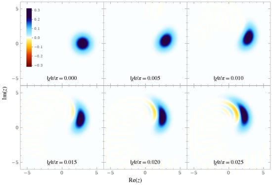
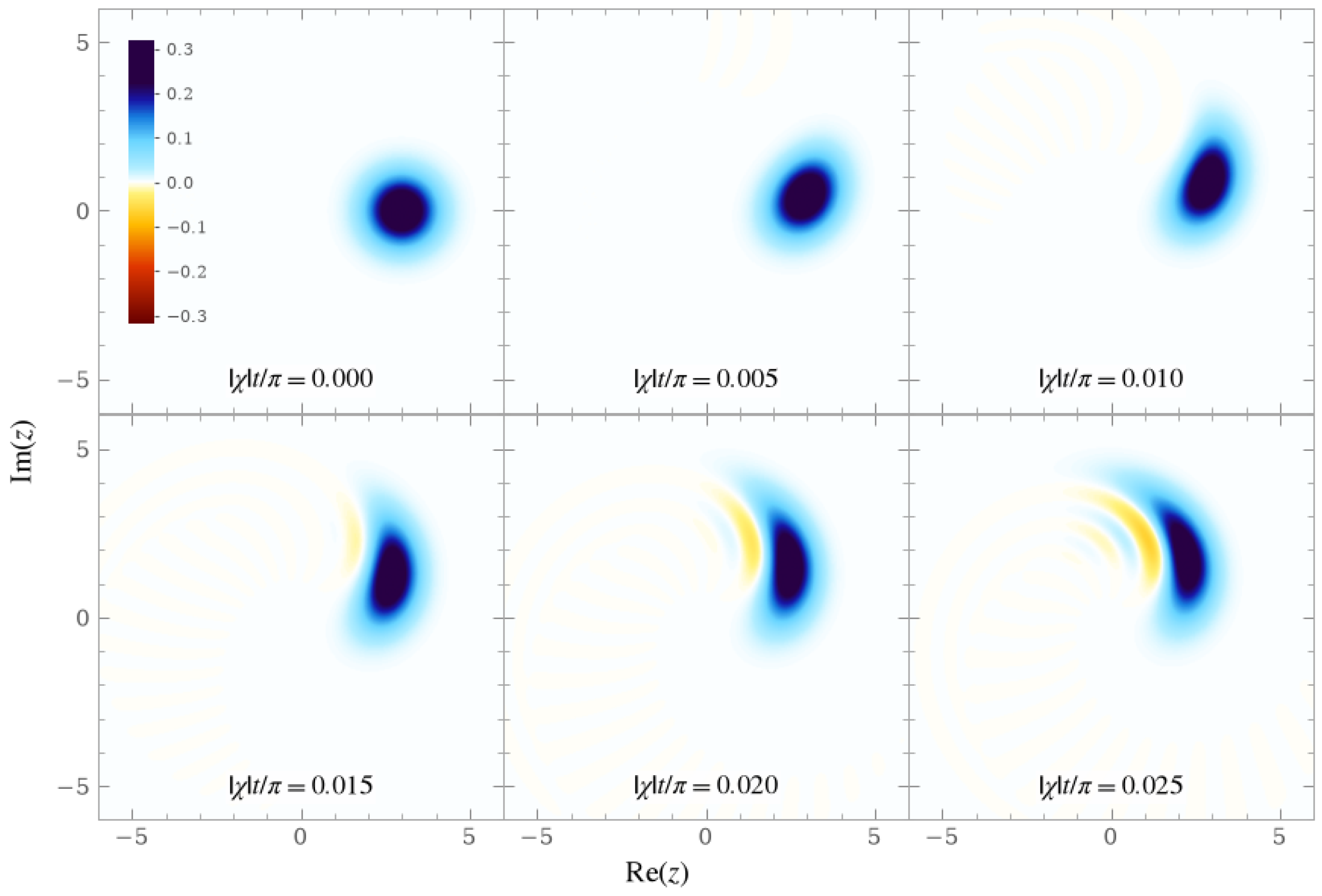
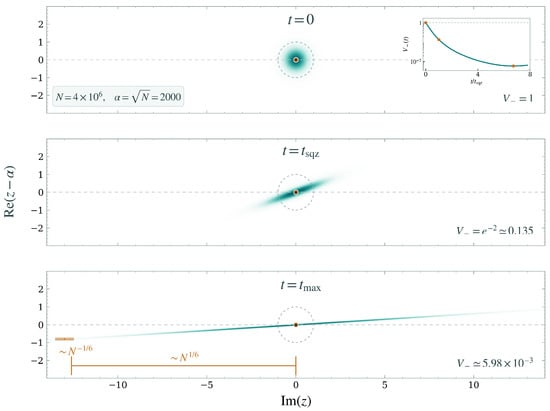
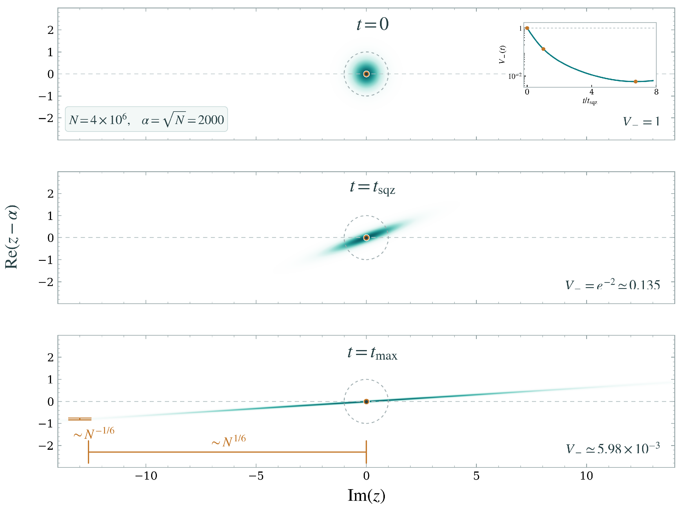
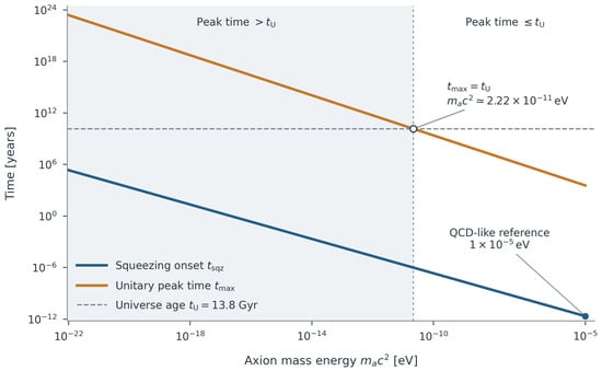
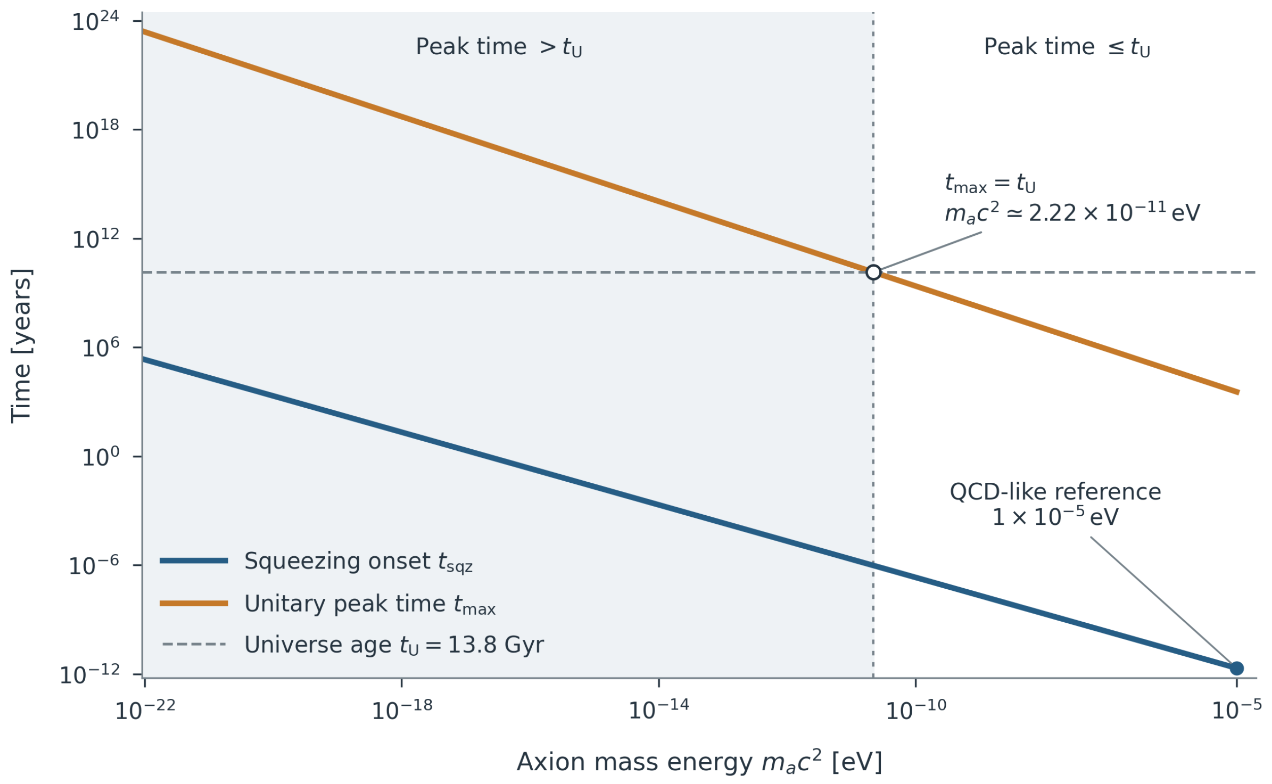
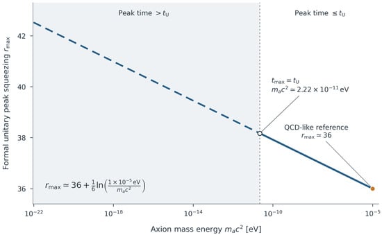
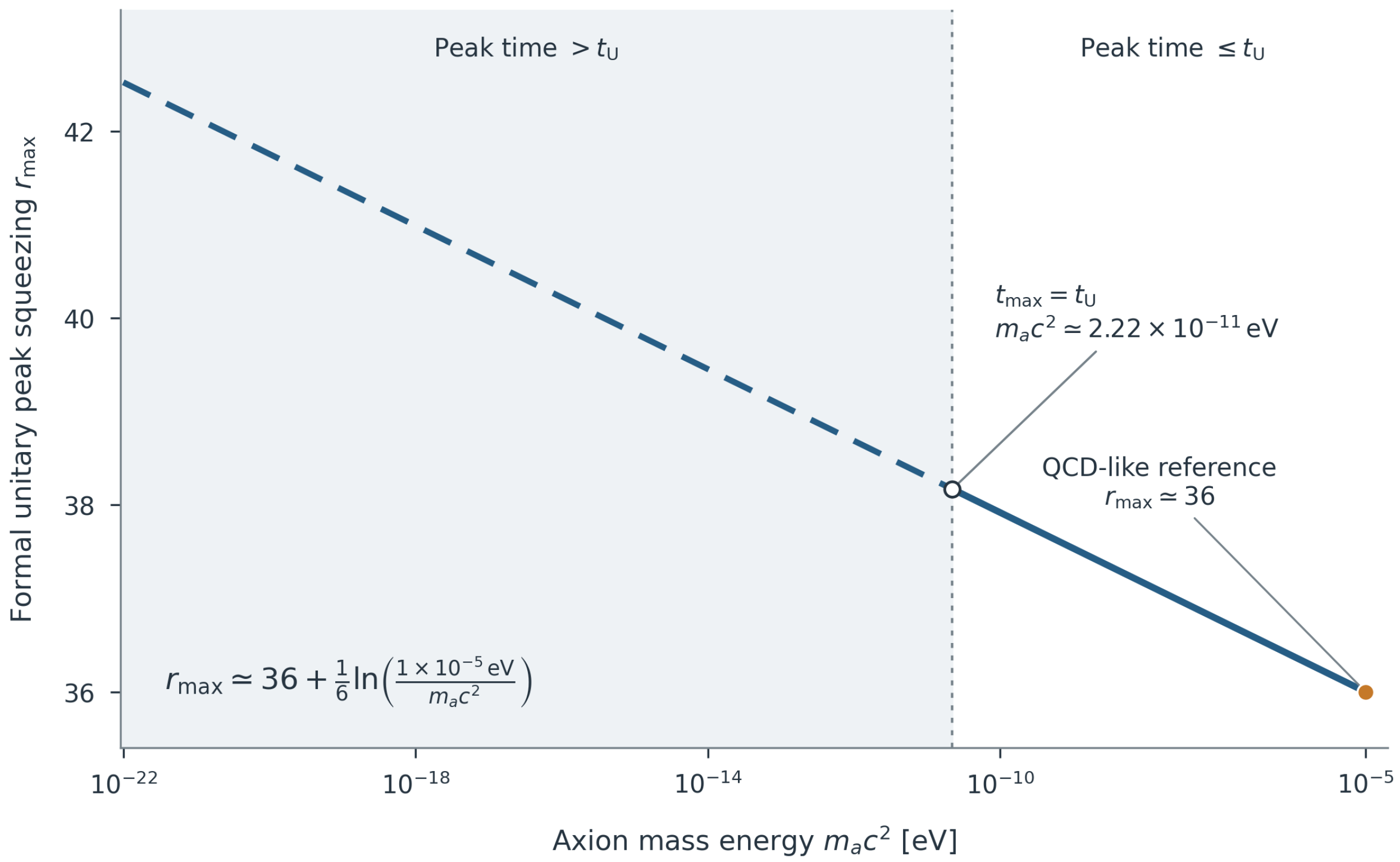
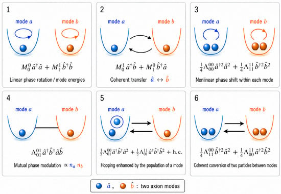
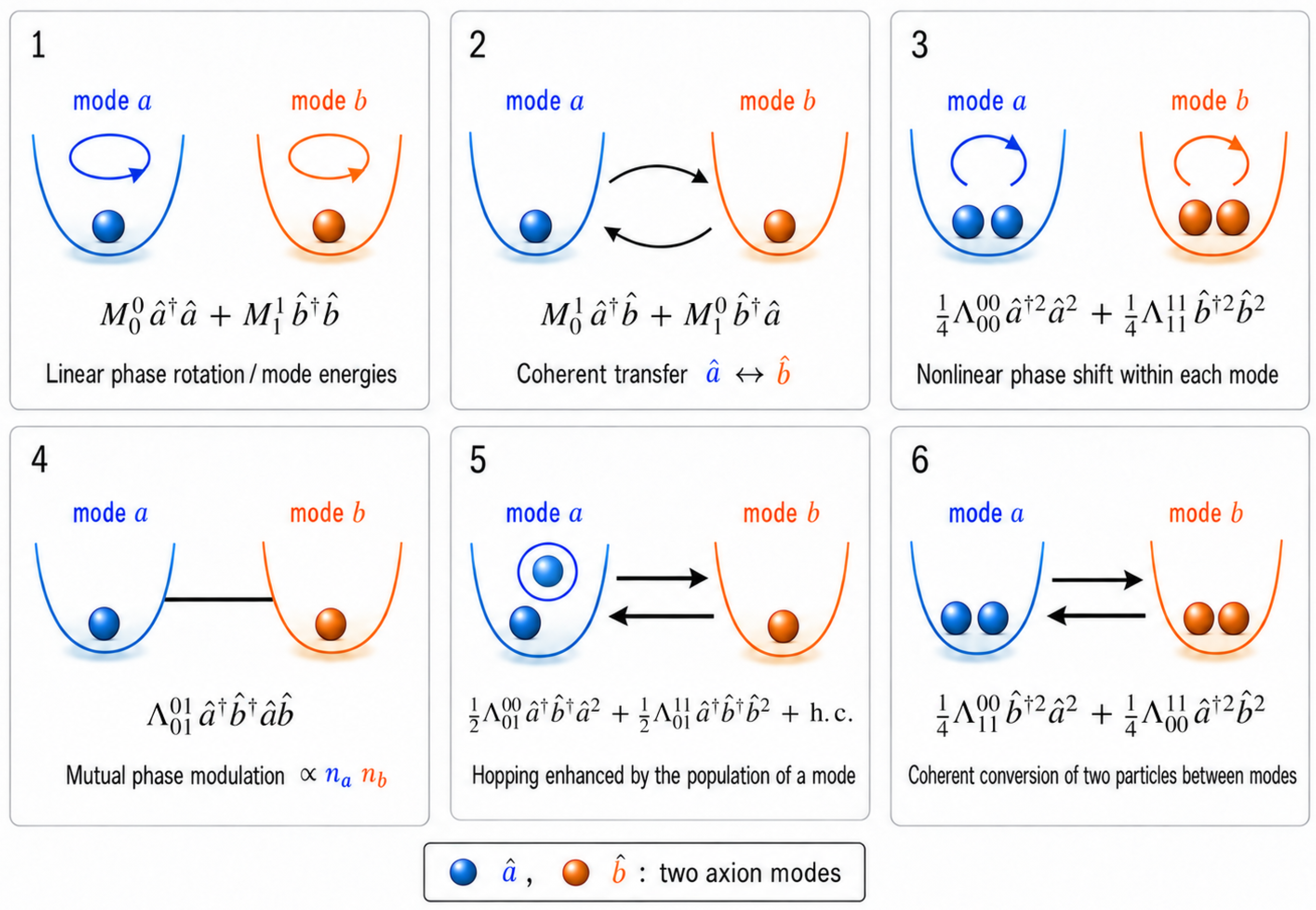
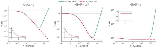
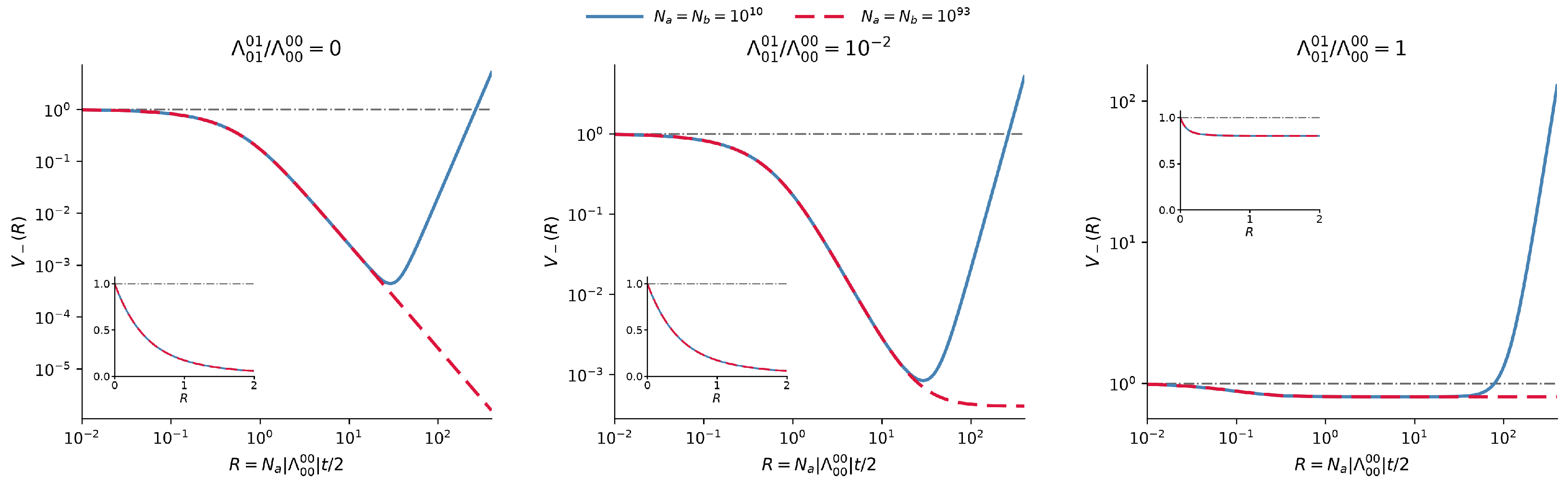
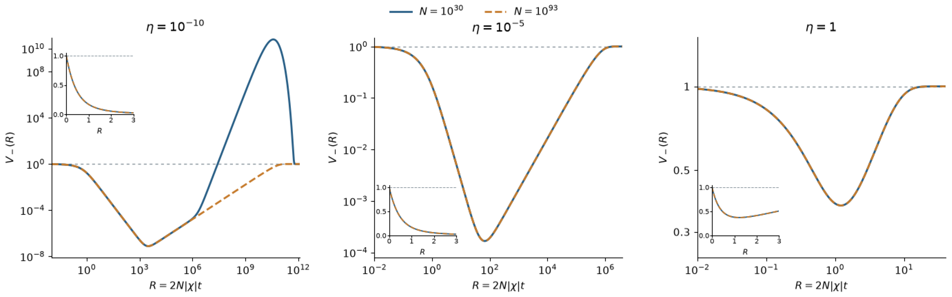
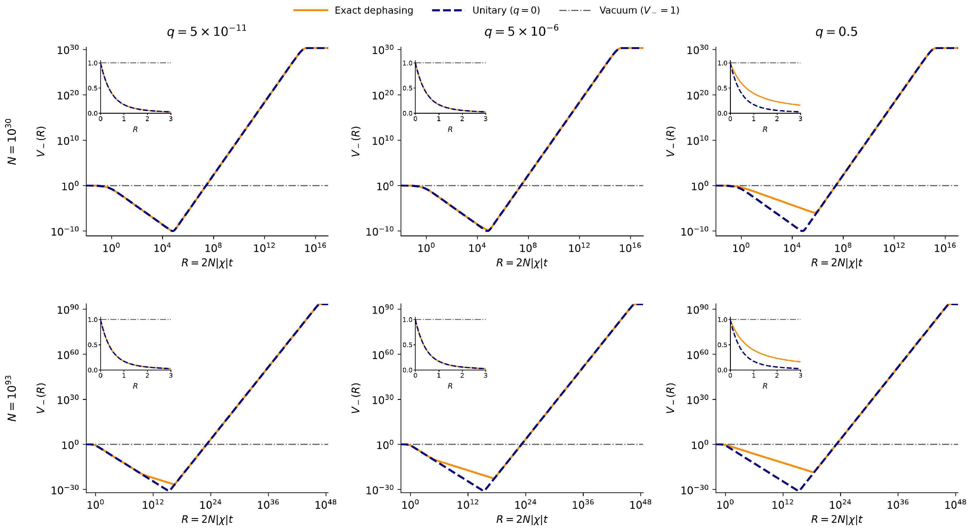
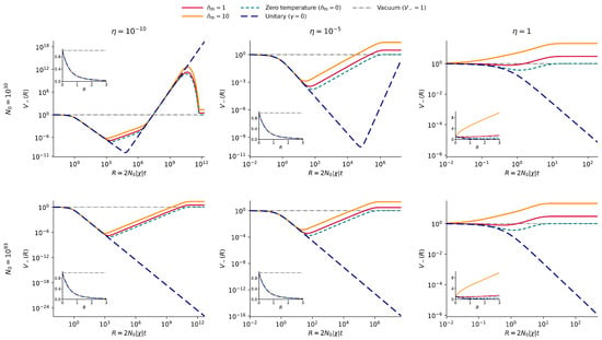
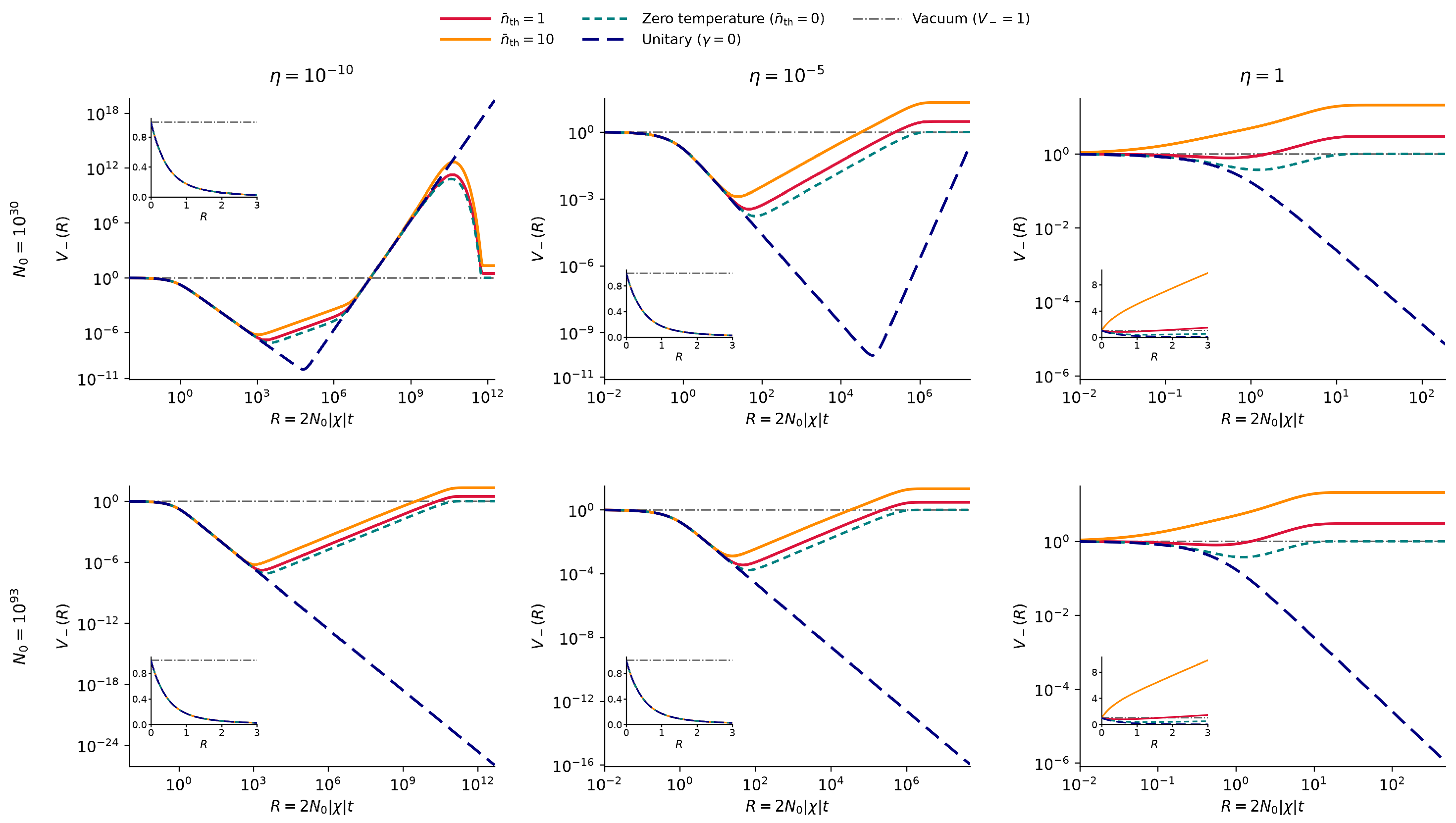
Disclaimer/Publisher’s Note: The statements, opinions and data contained in all publications are solely those of the individual author(s) and contributor(s) and not of MDPI and/or the editor(s). MDPI and/or the editor(s) disclaim responsibility for any injury to people or property resulting from any ideas, methods, instructions or products referred to in the content. |
© 2026 by the authors. Licensee MDPI, Basel, Switzerland. This article is an open access article distributed under the terms and conditions of the Creative Commons Attribution (CC BY) license.