


Abstract
Nested sampling is widely used in astrophysics and cosmology to reliably infer model parameters and compare models within a Bayesian framework. To address models with many parameters, Markov Chain Monte Carlo (MCMC) random walks are used within nested sampling to advance a live point population. Diagnostics for nested sampling inference are essential to verify that trustworthy astrophysical conclusions can be drawn. We develop a diagnostic to identify poorly mixed random walks that do not meet the requirements of nested sampling. The distance from the start to the end of the random walk, the jump distance, is compared to the typical neighbour distance between live points, to obtain a relative jump distance (RJD). A robust estimate of a typical neighbour Mahalanobis distance is obtained with the MLFriends algorithm. In mock and real-world inference applications such as inferring the distance to GW170817, we observe the relative jump distance. We propose the geometric mean <RJD> and fraction of RJD > 1 as new summary diagnostics. To evaluate the sensitivity of the new diagnostics, problematic runs are identified by comparison with reruns using much longer MCMC chains. Trustworthy inference runs are consistently associated with <RJD> above 1.1, while problematic runs can fall below these thresholds. The RJD is more sensitive than previous tests based on the live point insertion order. The RJD diagnostic is proposed as a widely applicable diagnostic to verify inference with nested sampling. It is implemented in the UltraNest package in version 4.1.
1. Introduction
Nested sampling [1,2] is a widely used algorithm in astrophysics and cosmology to infer model parameters and compare models within a Bayesian framework. To illustrate, the popular packages [3,4,5,6] have over 6000 citations1, supporting a wide range of astrophysical and cosmological analyses. One appeal of nested sampling is its robustness to complex parameter degeneracies, frequently encountered with sparse or limited observational data common in astrophysics.
Nested sampling achieves this by sampling a population of K live points from the prior probability distribution. Then, at each iteration, a live point is discarded and replaced with a new prior-sample, under the constraint that its likelihood must exceed the likelihood of the recently discarded point. This induces the behaviour of the live point population being distributed throughout the parameter space, but progressing towards the best fit. The key insight of [1] is that each iteration of nested sampling discards a constant fraction of the prior probability mass at each iteration, . The posterior distribution can be approximated by the discarded points, weighed by , where is the approximated prior probability discarded at iteration i, and is the likelihood of the discarded point. Then, the marginal likelihood is . For a more detailed introduction to nested sampling, see [2]. The classic error estimate considers the error, while [7] proposed bootstrapping of the live points to sample also the variance on . This Z error estimate is adopted here.
Several approaches have been proposed for prior-sampling under the likelihood constraint. The original proposal by [1] is to start a random walk from a live point for a number of steps M, and adopt the final point as a new live point. Points are accepted if they exceed the current likelihood threshold. Such step sampling nested sampling is the most efficient approach for models with many parameters (say, 20 or more). Slice sampling [8] was first adopted for nested sampling by [9] and popularized by PolyChord[4]. Various slice sampling approaches were compared by [10].
It is still unclear, however, how to choose the number of steps M. On the one hand, higher M induces a higher computational cost, which may be prohibitive. On the other hand, M must be chosen large enough so that the final point is sufficiently independent from the starting point (see also [11]). If M is too small, the inference result and thus scientific conclusions may be wrong. It is thus essential to recognize such problematic nested sampling runs with diagnostics.
Diagnostics for nested sampling can be divided into two categories: visualizations, such as trace plots [7], and tests, which this paper focuses on. If the true answer is known, such as in analytic test distributions, the prior mass shrinkage can be tested directly [12], as well as the final evidence and posterior samples. Typically, however, the true answer is not known. Here, we can distinguish tests that are generic or specific to the likelihood-restricted prior sampling technique. For generic tests, consistency of Z across reruns (e.g., [7,13]) is a basic check. However, consistency does not ensure a good run. Ref. [14] recognized that a newly sampled live point should be inserted into to likelihood-ordered list of live points in a random place. The distribution of insertion orders should be uniform, which is checked with a K-S test. Ref. [15] generalized this to the integer-based U-test, also applicable when the number of live points is changing during a run (dynamic nested sampling [16]). For nested sampling based on rejection sampling, importance nested sampling has been proposed as an alternative estimator [13,17]. Disagreement between the importance nested sampling estimator and the classic nested sampling estimator is a useful indicator with the sampling (see e.g., Feroz et al. [13], Nelson et al. [18]). For step samplers, comparing the Z estimate when doubling M is a powerful diagnostic [7,16]. A similar effect can be achieved by increasing the number of live points [19]. Such reruns with substantially enlarged M or K incur a large computational cost. It would therefore be beneficial to diagnose an inference run by itself, rather than in comparison with other runs. Such a diagnostic is presented in this paper.
2. Method
2.1. Background
Generalizing the idea of [14], newly sampled points should be unremarkable in all their properties compared to the existing live points. Here, we consider the proximity to the existing live points, and focus in particular on the distance to the live point where the random walk was started. This is motivated by the common failure mode that a walk is not diffusing far away from the starting point.
In nested sampling, the starting point is a randomly chosen live point. Across iterations, therefore, multiple newly sampled points can originate from the same live point. If the walk is not going far, a clump of points near that live point appears. This is then apparent in the distribution posterior sample as graininess of the distribution. Such graininess has the fundamental property that the distance between properly sampled live points is different than the distance of the random walk. We use this to develop a test.
A performance indicator proposed for Random Walk Metropolis (RWM) is the expected square jump distance (ESJD) [20]. It is defined as the mean square distance between one iteration and the next:
In particular, Pasarica and Gelman [20] consider some univariate variable of interest, such as one model parameter. Then, the square jump distance is simply . For a d-dimensional parameter position, the jump distance can be defined as the Euclidean distance. However, a local, decorrelated Mahalanobis distance may be more effective (see, e.g., clustering and affine transformations in [16]). In this more general case, with a covariance matrix , the jump distance (JD) is
To illustrate the behaviour of the ESJD, consider a RWM with a Gaussian proposal kernel. For a Gaussian proposal with a very small size, the ESJD is low. If the proposal kernel is too large, the Metropolis rule rejects most proposals and the chain remains stuck, again making the ESJD low. Based on this, Ref. [20] optimizes the kernel scale to maximize the ESJD. The ESJD is inversely related to the first-order auto-correlation of the random walk [20], which should be minimized for effective diffusion far away from the starting point. This inverse relationship means that maximizing the jump distance is equivalent to minimizing the autocorrelation time of the Markov chain, which is the standard criterion for efficient mixing. In the context of nested sampling, where the chain must produce a new live point that is effectively independent of the starting live point, good mixing (large jump distance relative to the live point distribution) is therefore a necessary condition for the validity of the step-sampling approach, even though it is not on its own sufficient to guarantee a correct result.
In the context of nested sampling, Ref. [11] suggested optimizing the expected square jump distance (ESJD) with trial walks. Trials would need to be conducted at each nested sampling iteration, because the distribution is changing with each nested sampling iteration. Specifically, the prior volume becomes exponentially smaller.
2.2. Relative Jump Distance
Here, we develop a new diagnostic by relating the jump distance to the typical distance between live points. This normalization is essential for nested sampling, because the sampled geometry, constrained by the evolving likelihood constraint, is changing in each iteration: early in the run, the live points span nearly the full prior volume, while late in the run, they may be confined to a tiny region of parameter space. Without normalization, a raw jump distance that appears large in absolute terms may in fact be small relative to the current scale of the live point distribution, and vice versa. By dividing the jump distance by a robust estimate of the typical inter-point separation, the relative jump distance provides a scale-invariant measure of chain mixing that is directly comparable across all stages of a nested sampling run and across problems of different dimensionality.
We define a reference distance to put the JD in context. The reference distance should be a typical distance between live points. Following other works, for the numerical experiments in this paper, we work in a coordinate system defined in natural prior probability units (unit hypercube), and apply clustering and an affine whitening transformation that makes the live point sample covariance the unit diagonal matrix (see e.g., [6,10,21]). This already provides a first normalization of the jump distances. This is however insufficient, because the sample covariance is not equal to the covariance of the likelihood-restricted prior, and the likelihood-restricted prior may be more complex than an ellipsoidal distribution. To address the structure of the likelihood-restricted prior contour and its dimensionality-dependent edge behaviour, one can consider several choices, such as the typical nearest neighbour distance of the live points. However, complex likelihood-restricted prior geometries can make the nearest neighbour distance distribution multi-modal and therefore, the mean and median nearest neighbour distance are unstable.
For a robust computation, we adopt as the reference distance the radius computed by the MLFriends algorithm [12,22], as computed for example by dynesty and UltraNest. This is found by splitting the live points into a training sample by bootstrapping (sampling with replacement), and a complementary test sample of the left-out points, and identifying the nearest training point for each test point. The MLFriends radius r is then the maximum over all these nearest distances across B bootstrapping rounds. Here, we adopt B = 30. Appendix A presents Python 3 code to compute r. A detailed analysis of the MLFriends algorithm is presented in [23], but we briefly summarize the behaviour. The neighbourhood defined by radius r is large enough to include live points that may be absent due to the Binomial Point Process sampling of the likelihood-restricted prior, and is thus expected to encompass the next live point across B bootstrap rounds. Unlike a radius derived purely from the Binomial point process alone, which would only account for the average number density of live points, r adapts to the local geometry of the prior space, making it a meaningful measure of the characteristic distance between live points, and therefore it is suitable as a reference distance.
For the simplified mono-modal case of ellipsoidally distributed live points, Appendix A investigates the dependence of r on dimensionality and the number of live points, and finds a Mahalanobis distance of in high dimensions. This is likely related to the “concentration of distances” effect (see e.g., [24], for a review).
With the reference distance r in hand, we define the relative jump distance as
The threshold RJD = 1 has a natural geometric interpretation: a jump of distance equal to r means the new point has moved at least as far as the typical nearest-neighbour spacing among live points, suggesting it has explored a meaningfully different region of the constrained prior. Jumps with RJD < 1 indicate the new point lies closer to its starting point than to the nearest other live point, a sign of poor chain mixing. By definition of the bootstrapped r, multiple live points lie within the radius r. We therefore expect for the majority of jumps, if the walk is effective.
2.3. Summary Statistics
We observe the distribution of RJDs over the nested sampling run. To summarize the distribution, we track the fraction of jumps that exceed the reference distance () and the geometric mean RJD. As shown below, the RJD distribution is often log-normal. Problematic runs have a low-RJD tail. The geometric mean highlights such a tail better than an arithmetic mean or median, which would be dominated by the unproblematic large RJDs.
The RJD can also be bimodal. Consider for example a banana geometry in two dimensions. If there are enough live points, r describes the typical nearest neighbour distance, insensitive to the length of the banana. A good random walk traverses across the banana. A poor walk, with proposals only orthogonal to the banana, is stuck and only traverse approximately the width. The fraction of far jumps, , diagnoses the ratio between good and poor proposals.
3. Results
We show the behaviour of our new diagnostic in several applications, which are specified by a d-dimensional prior probability distribution and a likelihood function. These applications range from standard mathematical test problems to a real gravitational wave parameter estimation problem, demonstrating the relevance of the diagnostic across the spectrum of problems encountered in astrophysics. For each application, we run nested sampling with 400 live points until the dead points contain more than one per cent of the total estimated posterior weight. A sequence of runs is performed with d, , , , etc., number of steps, where d is the number of model parameters. For some problems, we start from . For simplicity and to clearly show the behaviour, we use a slice sampler that proposes along one randomly chosen parameter axis. The seed is fixed across runs.
3.1. Gaussian
Integration of a Gaussian likelihood is a standard test problem: . The true marginal likelihood is . We adopt standard uniform priors with d = 4, d = 16 and d = 100.
The variation adopted here has different standard deviations for each parameter:
where , so that ranges from to , with equal total information across dimensionalities where the floor is not active. Additionally, the means are varied, avoiding a special place (such as the centre) of the prior:
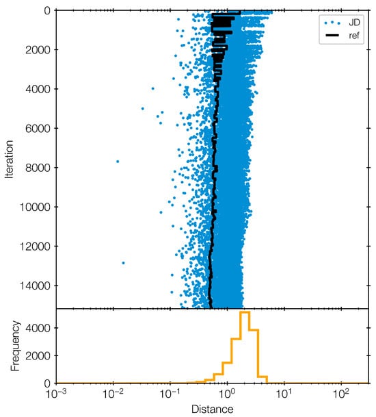
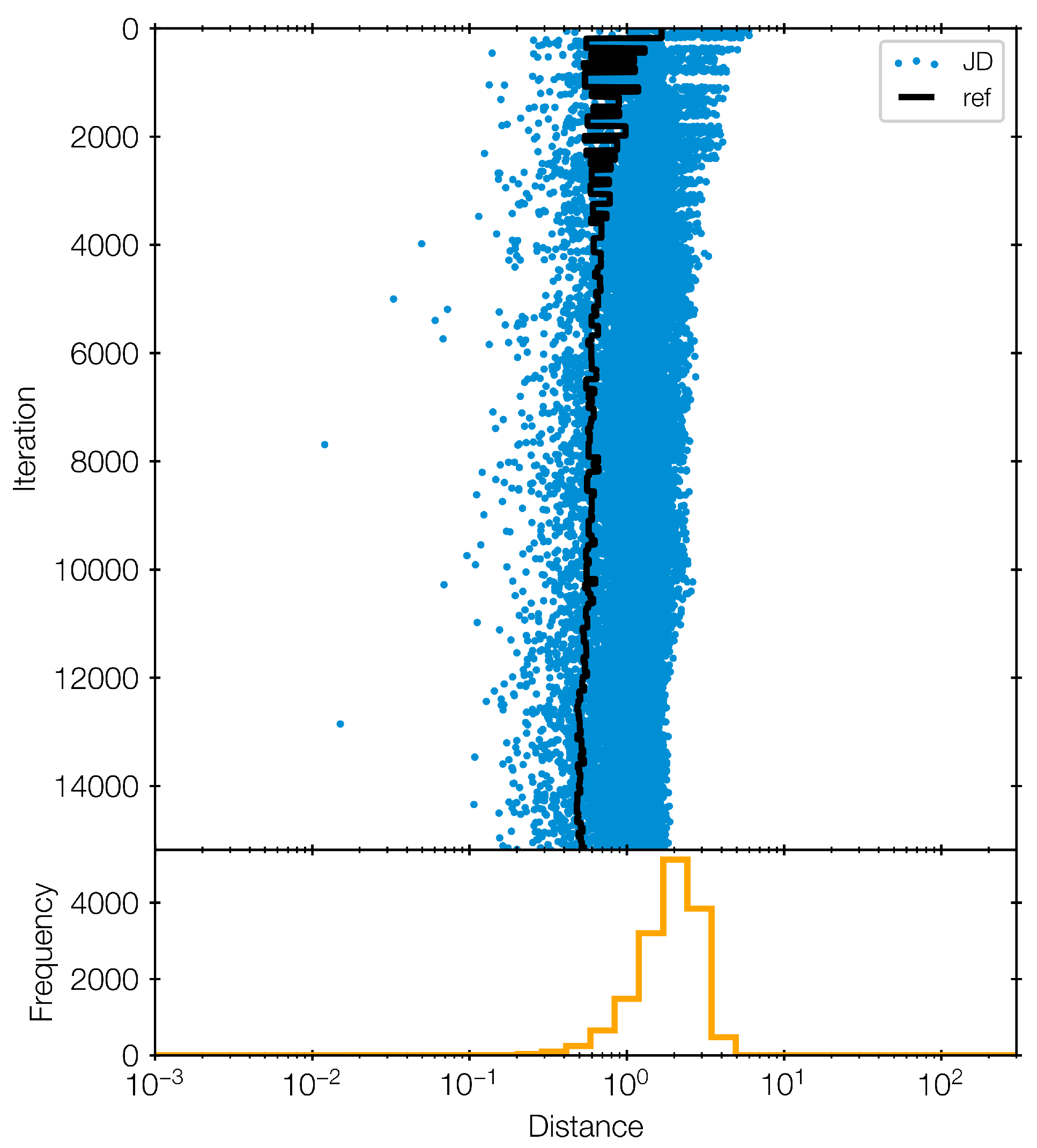
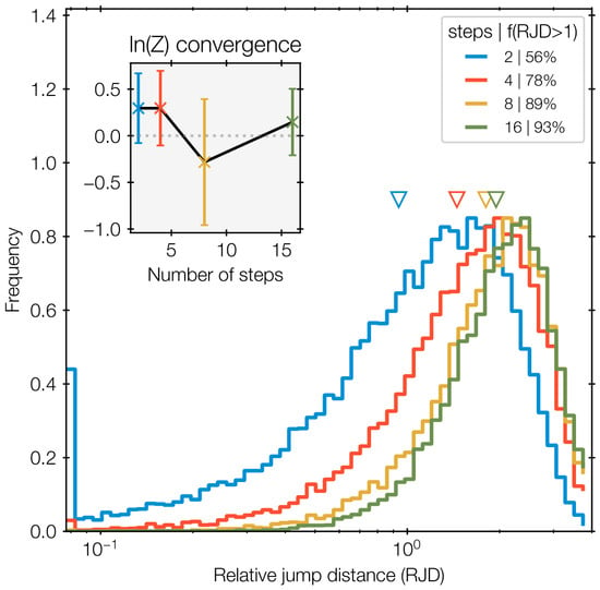
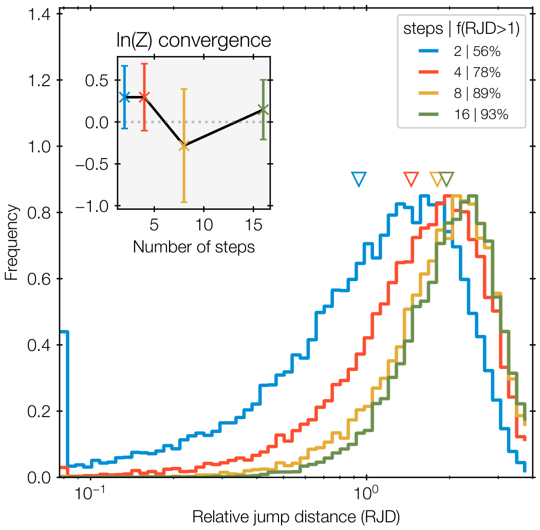
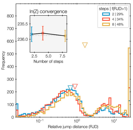
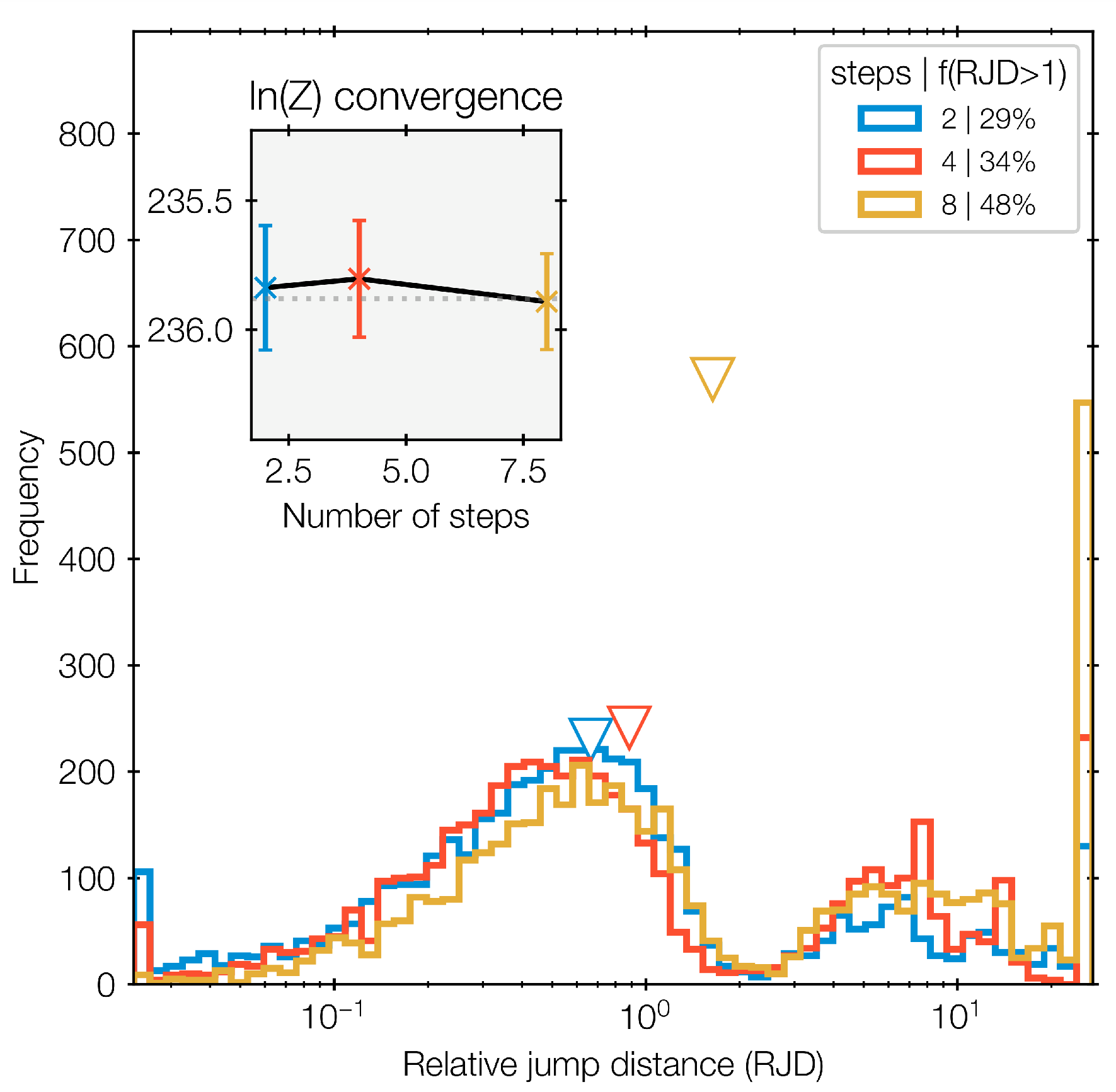
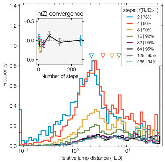
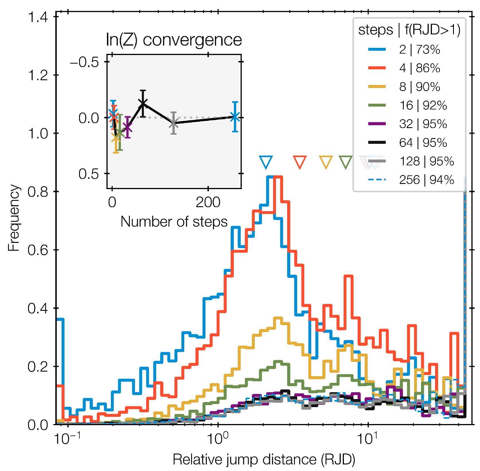
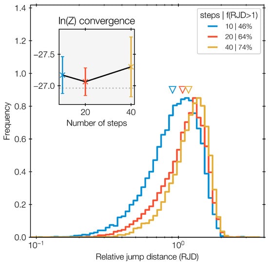
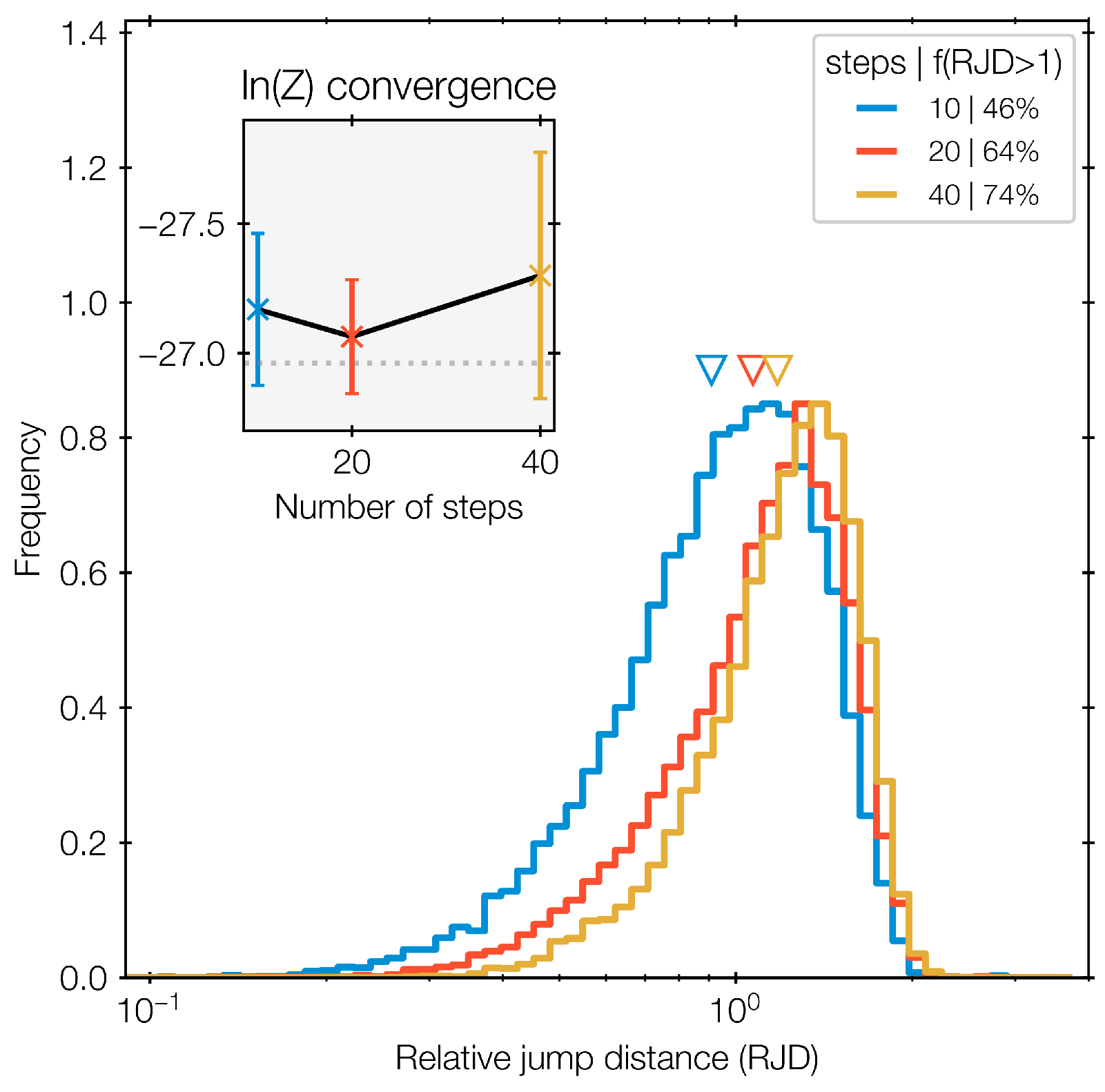
The jump distances of a nested sampling run with d = 4 is shown in Figure 1. The JD for each iteration are shown as blue dots and the reference distance r in black, both in whitened coordinates. r is close to 0.5 throughout. The bottom panel shows the RJD distribution. Figure 2 shows the RJD distribution for all runs across number of steps. With M = 4 steps (blue histogram), the distribution is shifted to the left compared to the histograms with more steps. In all distributions, the majority have RJD > 1 (see figure legend), and the geometric mean RJD is also above 1. The inset in Figure 2 presents the corresponding ln(Z) estimates from results from runs with different M. These vary around the true value (0). Here, both the ln(Z) calibration and the RJD distribution indicate acceptable runs.
Figure 1.
Top panel: Jump distance (blue) and reference Mahalanobis distance (black) at each nested sampling iteration for the run with M = 8 steps. Most blue points are to the right of the black curve, i.e., JD > r. Bottom panel: The histogram of the ratio (relative jump distance, JD/r). The majority lies mostly above 1.
Figure 2.
Gaussian test likelihood run diagnostics. The inset shows evidence estimates (y-axis) for a sequence of nested sampling runs with different number of steps (x-axis). The RJD distribution for each is shown in the main panel. The distribution is bell-shaped in logarithmic units, but has a low-end tail, which is more pronounced when the number of steps is smallest (blue). The fraction of RJD > 1 is given in the legend with the number of steps. The geometric mean of RJDs for each run is shown near the respective histogram with the same colour with downward-pointing triangles. Here, the means are all above 1 and the fractions above 50 per cent.
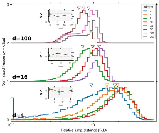
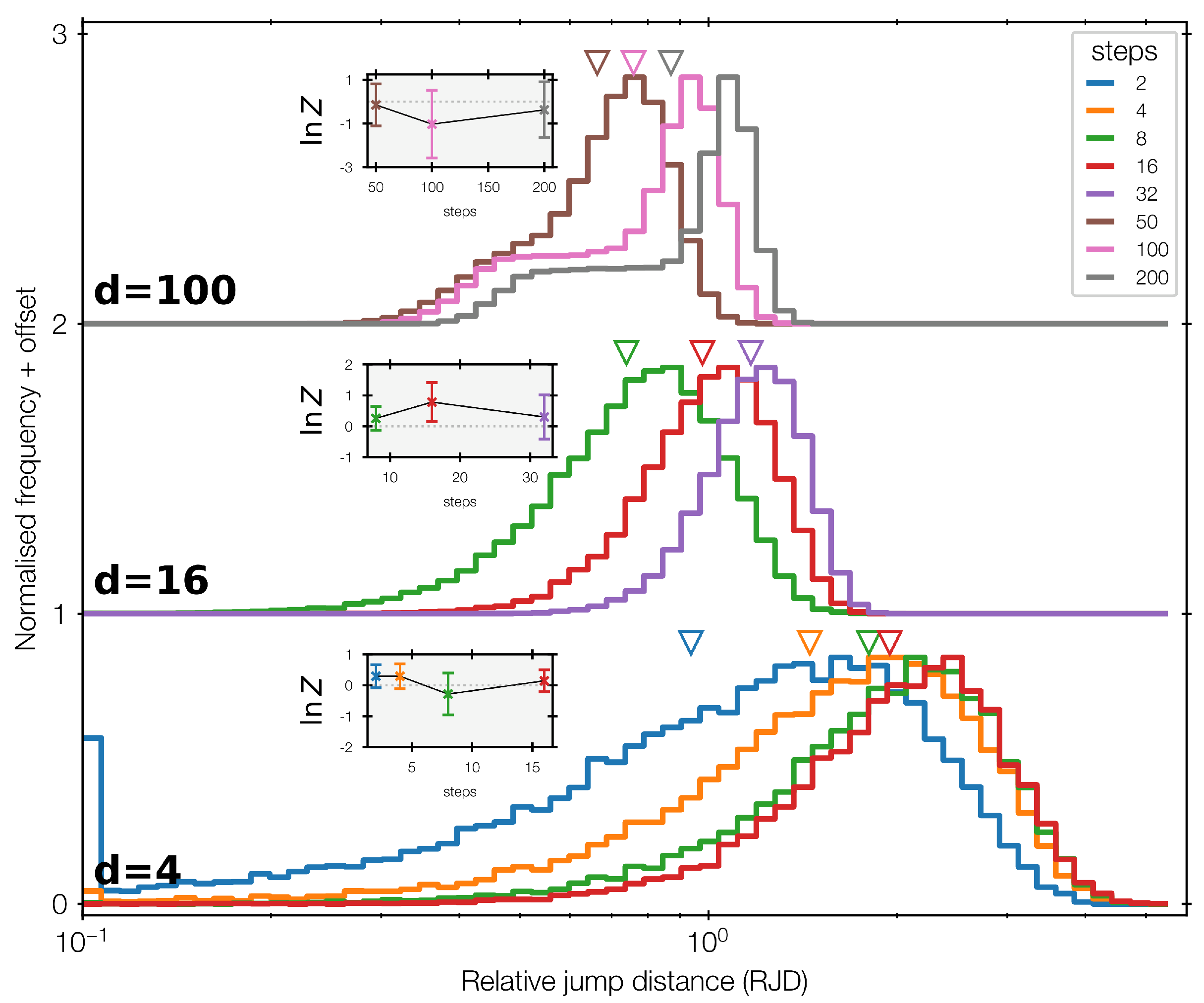
Figure 3 shows a comparison of the d = 4, d = 16 and d = 100 cases. Here, we start from d/2 number of steps. The evidence error bars are all overlapping, indicating that the runs do not change with increased number of steps. Nevertheless, for each case, the histograms change with the number of steps, with the geometric means moving towards the right in lockstep, and the fraction of RJD > 1 increasing. The RJD distribution shapes are very different from each other. While d = 4 and d = 16 are bell curves with a strong tail at the low end, the d = 100 case features a plateau. This is likely due to the many initial iterations where the likelihood-restricted prior still covers the entire unit prior length in many of the parameters. In these iterations, the geometry is thus similar to a box.
Figure 3.
The bottom histogram is the same as Figure 2 for the d = 4 Gaussian. This also includes M = 2 steps. The offset additional histograms (and corresponding insets) show the d = 16 and d = 100 case.
3.2. Box
We investigate a 5-dimensional non-ellipsoidal likelihood on a standard uniform prior. This is a sharply truncated Gaussian likelihood: , where is the parameter with the largest deviation from zero.
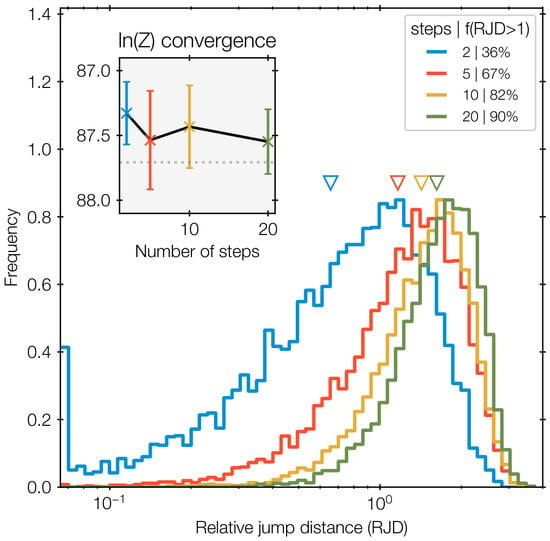
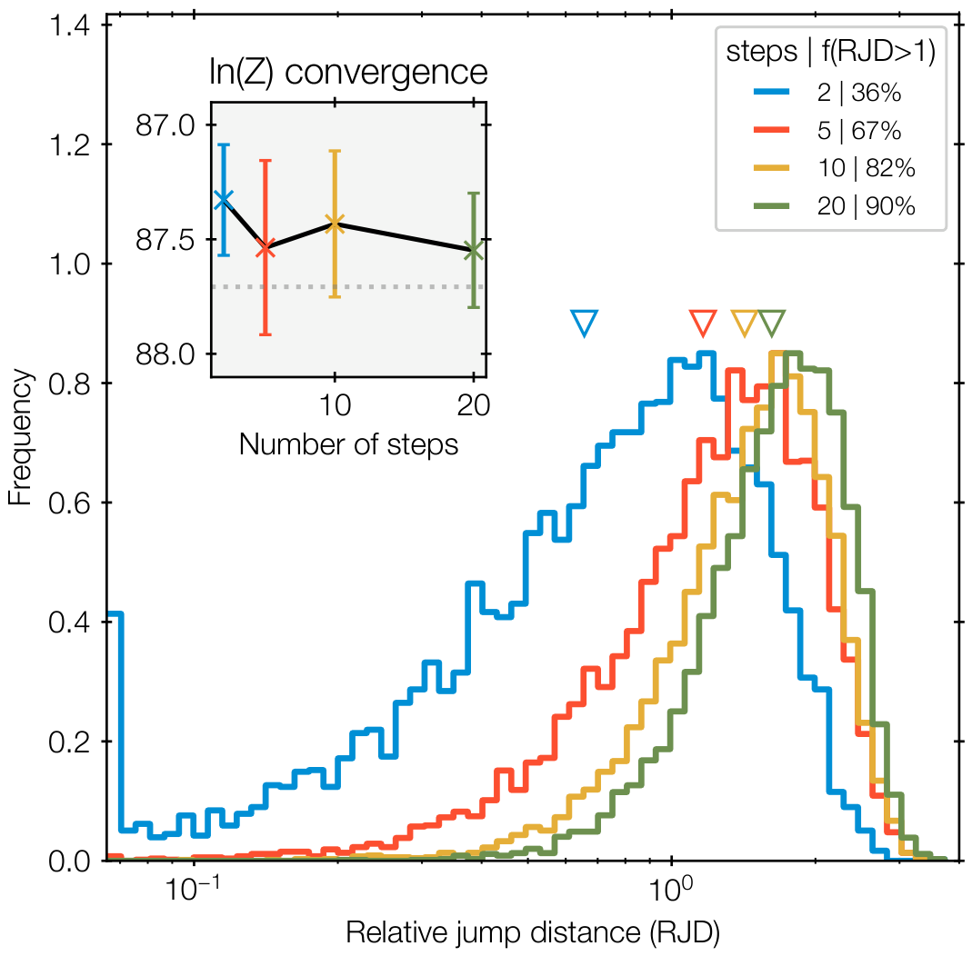
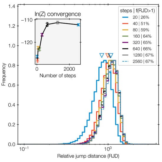
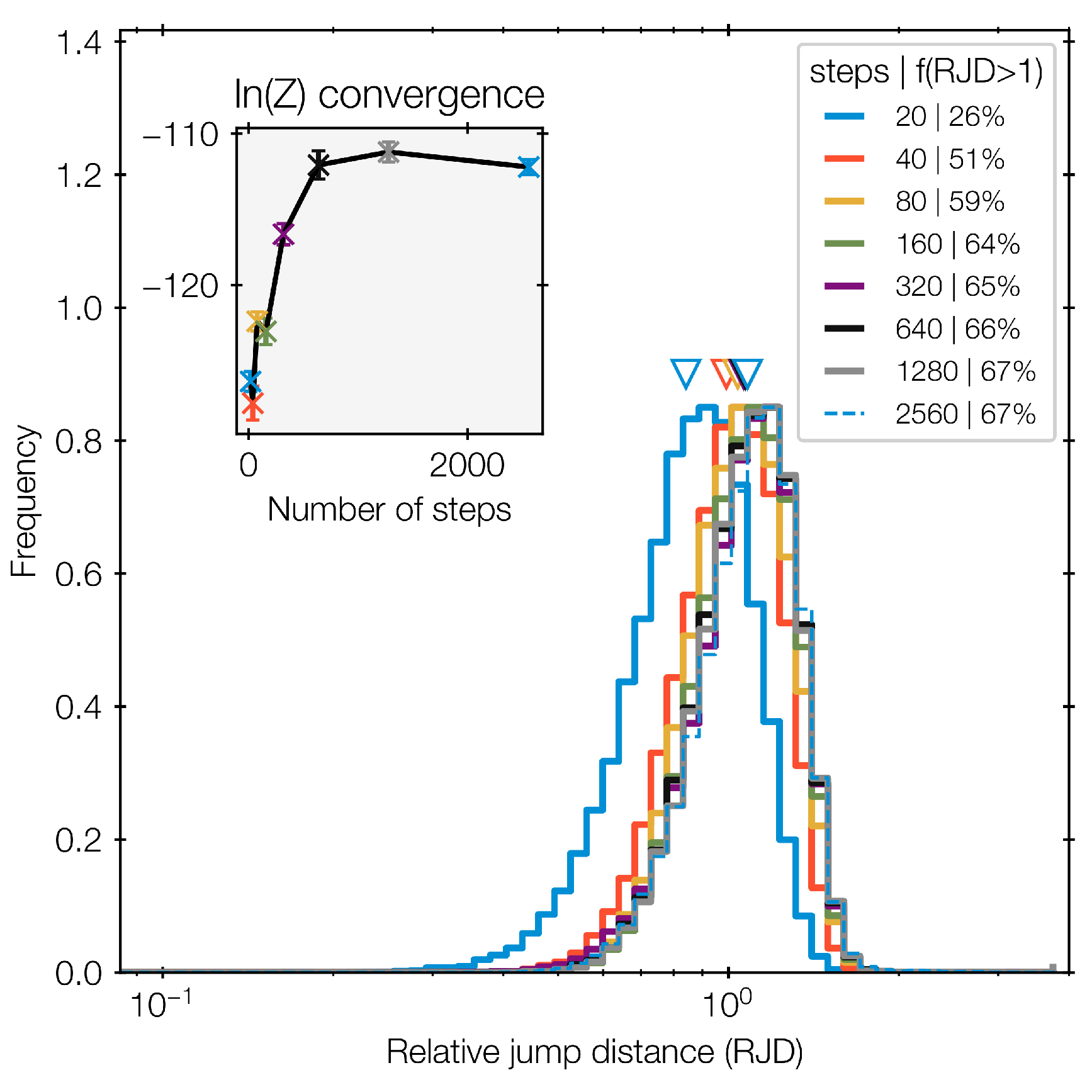
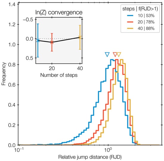
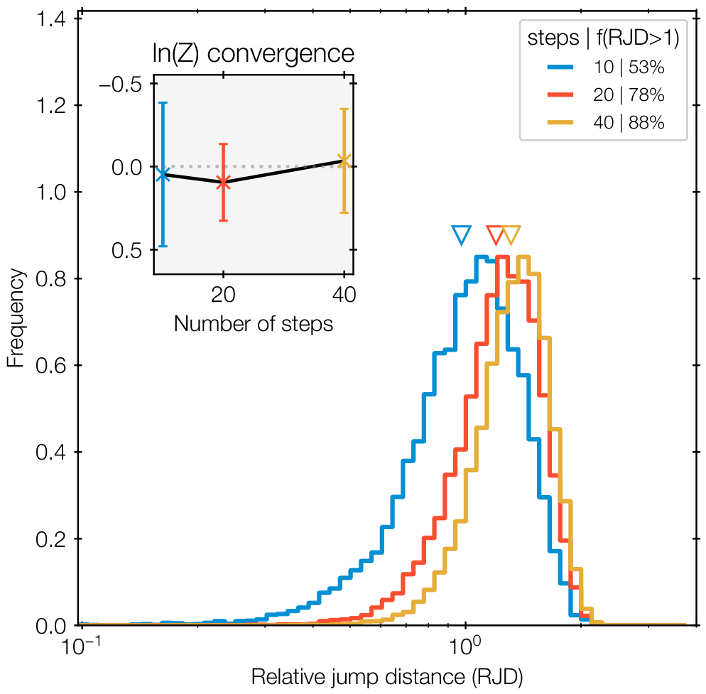
The inset of Figure 4 shows little difference in evidence estimates with increasing number of steps. The first error bar is however not overlapping with the true value, . However, the histograms of RJD in Figure 4 shift progressively toward higher values the more steps are used. With 20 steps, the vast majority of steps are at RJD > 1.
Figure 4.
Same as Figure 2, but for a 5d box.
3.3. Rosenbrock Function
We next consider a higher-dimensional, and non-linearly degenerate likelihood. The Rosenbrock function is a standard test problem in optimization. It exhibits a banana-like degeneracy that can be difficult to navigate. We adopt the formulation with uniform priors between −10 and +10 for each parameter.
For d = 2, the main panel of Figure 5 shows a mild decrease in evidence estimates with number of steps, and the RJD histograms on the right are comparable. Most RJD are above 1. The d = 20 case is more interesting. The inset of Figure 6 shows a strong change in evidence estimates as the number of steps is increased. Arguably, the result is not converged at fewer than 500 steps. The RJD histograms on the right also moves to the right with increasing number of steps; however, the effect is subtle from 40–180 steps. The mode of the RJD distribution is just above 1.
Figure 5.
Results from the banana-like Rosenbrock likelihood in 2d. Same as Figure 2.
Figure 6.
Same as Figure 5, but for the Rosenbrock likelihood in 20d. The RJD distribution (main panel) is bell-shaped in logarithmic units and shifts to the right with increased number of steps. The evidence estimate (inset) increases with the number steps until M = 640.
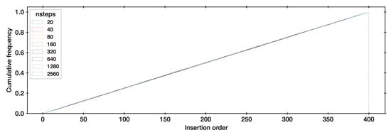
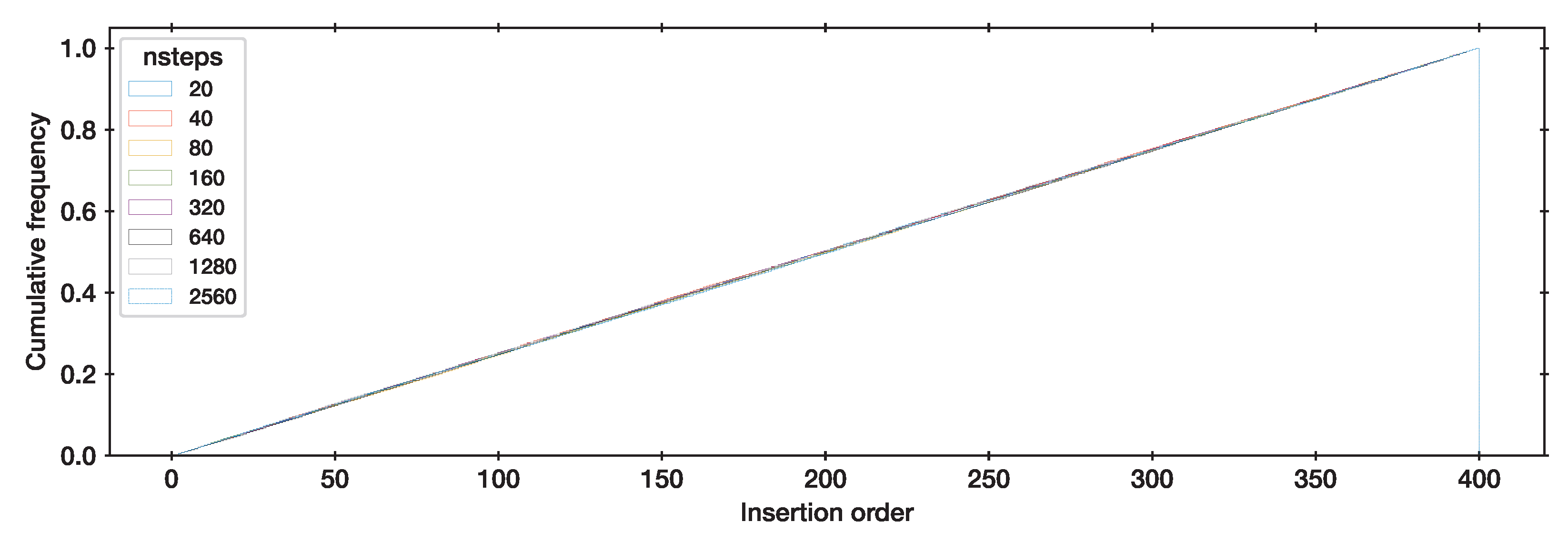
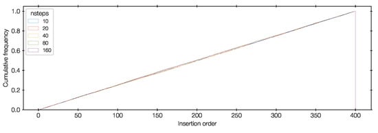
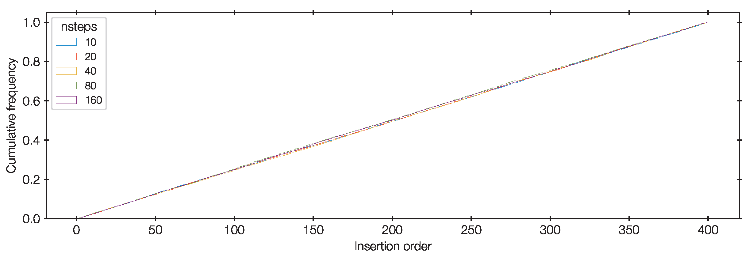
To complement these results, we also investigate the effectiveness of the insertion order statistic. Figure 7 presents a cumulative histogram of the insertion orders, which is indistinguishable from a uniform distribution. At all number of steps, neither the U test nor the KS test raises alarm about the results (p > 0.01).
Figure 7.
Insertion order distribution for Rosenbrock runs in Figure 6. In all cases, the deviation from a uniform distribution is insignificant (p > 0.01).
3.4. Eggbox
To investigate multi-modality, we adopt the two-dimensional Eggbox likelihood from [25]. It is defined as with uniform priors for each parameter between 0 and .
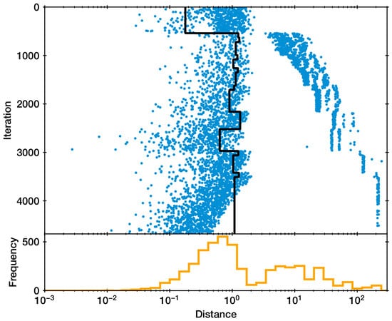
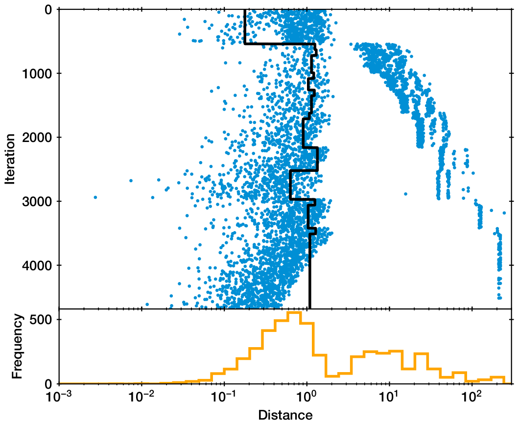
Here, the observed jump distances have a complex behaviour. Figure 8 shows the jump distances for a nested sampling run. Initially, the reference distance is indicating a typical neighbour distance of the uniformly distributed prior samples. After 500 iterations, the live points concentrate so that clusters can be identified, i.e., r indicates a typical distance within each cluster (r∼1). Some jumps are still possible across clusters (JD >> 1), while most remain within (JD∼1). This leads to a bimodal distribution in RJD. The emerging RJD histograms on the bottom is then bimodal. Figure 9 compares the RJD histograms for runs with different number of steps. The evidence estimates in the inset of Figure 9 show no significant variations.
Figure 8.
Same as Figure 1, but for the Eggbox likelihood analysed with M = 8 steps. The reference distance (black curve) is low in the first 500 iterations, and most jump distances (blue dots) are larger. In the middle, the reference distance is near 1, and the jump distances are either near 1 or above 10. The bottom panel shows the resulting bimodal RJD distribution (orange histogram).
Figure 9.
The RJD distribution for the eggbox likelihood is bimodal for all three runs (main panel). The evidence estimates in the inset are consistent within the error bars.
3.5. LogGamma
A difficult multi-modal, non-ellipsoidal problem was introduced by [26], and is defined as
We test this problem in 2 and 10 dimensions, with parameters assigned standard uniform priors. The true marginal likelihood is Z = 1.
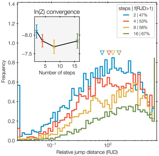
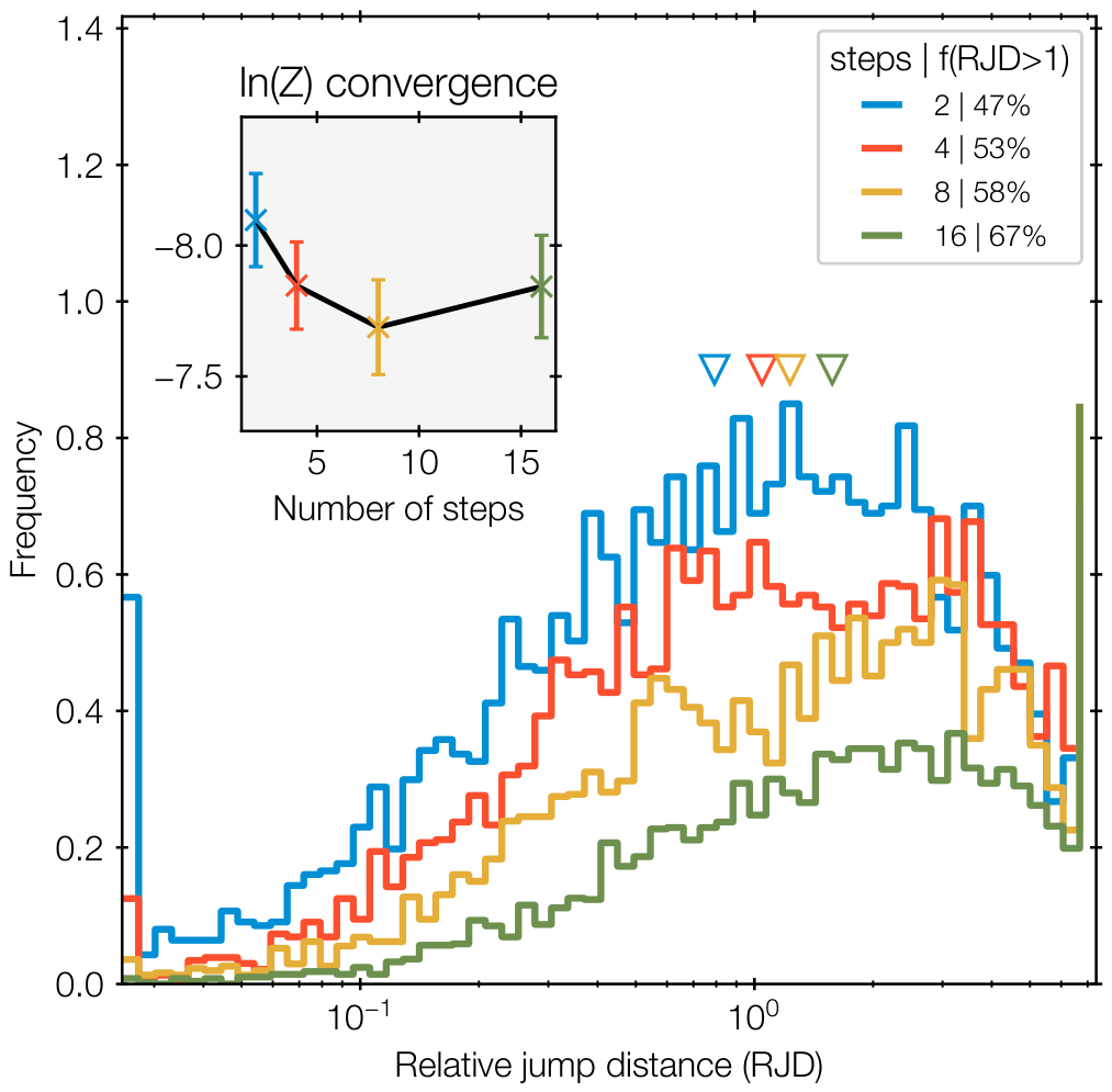
The RJD histograms in Figure 10 is again complex, similar to the Eggbox. Going from the M = 2 (blue histogram) and the M = 8 case, a tail at low RJD disappears and a hump at gains prominence. The latter is presumably related to jumps between modes. The evidence estimates are similar (ln(Z) = 0.1) and very close to the true value (0).
Figure 10.
LogGamma likelihood in 2d. The RJD distribution (main panel) is bimodal at high number of steps. The tail at RJD < 1 is more pronounced at the lowest number of steps.
At higher dimensions, the evidence estimates are consistent with the true value (0) for runs with 20 steps or more (inset of Figure 11). For 10 steps, the evidence is potentially over-estimated, however. Reruns with a different seed gives evidence estimates near zero for all M, indicating that the evidence trends are not significant. The main panel of Figure 10 shows that the histogram with 10 steps has the majority of RJD below 1, while at a higher number of steps, the vast majority are above 1.
Figure 11.
The RJD distribution for the LogGamma likelihood in 10d is bell-shaped in logarithmic units and shifts to the right with increased number of steps. The results with 40 and 80 steps are very similar. The evidence estimates in the inset converge to the true value (0) at approximately 40 steps, although all error bars overlap with each other. At 20 steps or higher, the geometric mean indicated by the downward-pointing triangles lies above 1, and the fraction of RJD > 1 (listed in the legend) are above 75 per cent.
3.6. Funnel
Neal’s funnel [8] is a standard test problem that represents features of hierarchical Bayesian models. Here, we adapt the correlated version of [27] with a correlation matrix M with diagonal elements and off-diagonals set to . Then, the Gaussian likelihood is
with the standard deviation and locations being model parameters. The sampled parameters are and scaled deviations , such that (noncentred parameterization). We assign a standard normal prior to and uniform priors between −10 and 10 for each . This problem is tested in 10 dimensions (i.e., i from 1 to 9). The marginal likelihood, from numerical integration along the parameter and analytic marginalization of the other parameters, is .
Figure 12 shows that the vast majority of RJD values lie above 1 if more than 10 steps are used. The evidence estimates in the inset are confined to a narrow range with error bars overlapping with the true value. Figure 13 shows a histogram of the insertion order distribution. These are indistinguishable from a uniform distribution for all cases. Of these three plots, the RJD distribution appears most sensitive to the number of steps.
Figure 12.
Funnel likelihood in 10d. Same as Figure 2.
Figure 13.
Insertion order distribution for Funnel runs in Figure 12. In all cases, the deviation from a uniform distribution is insignificant (p > 0.01).
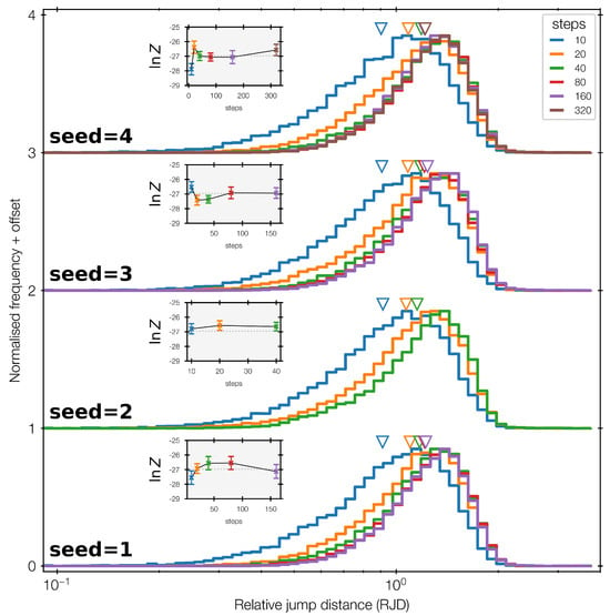
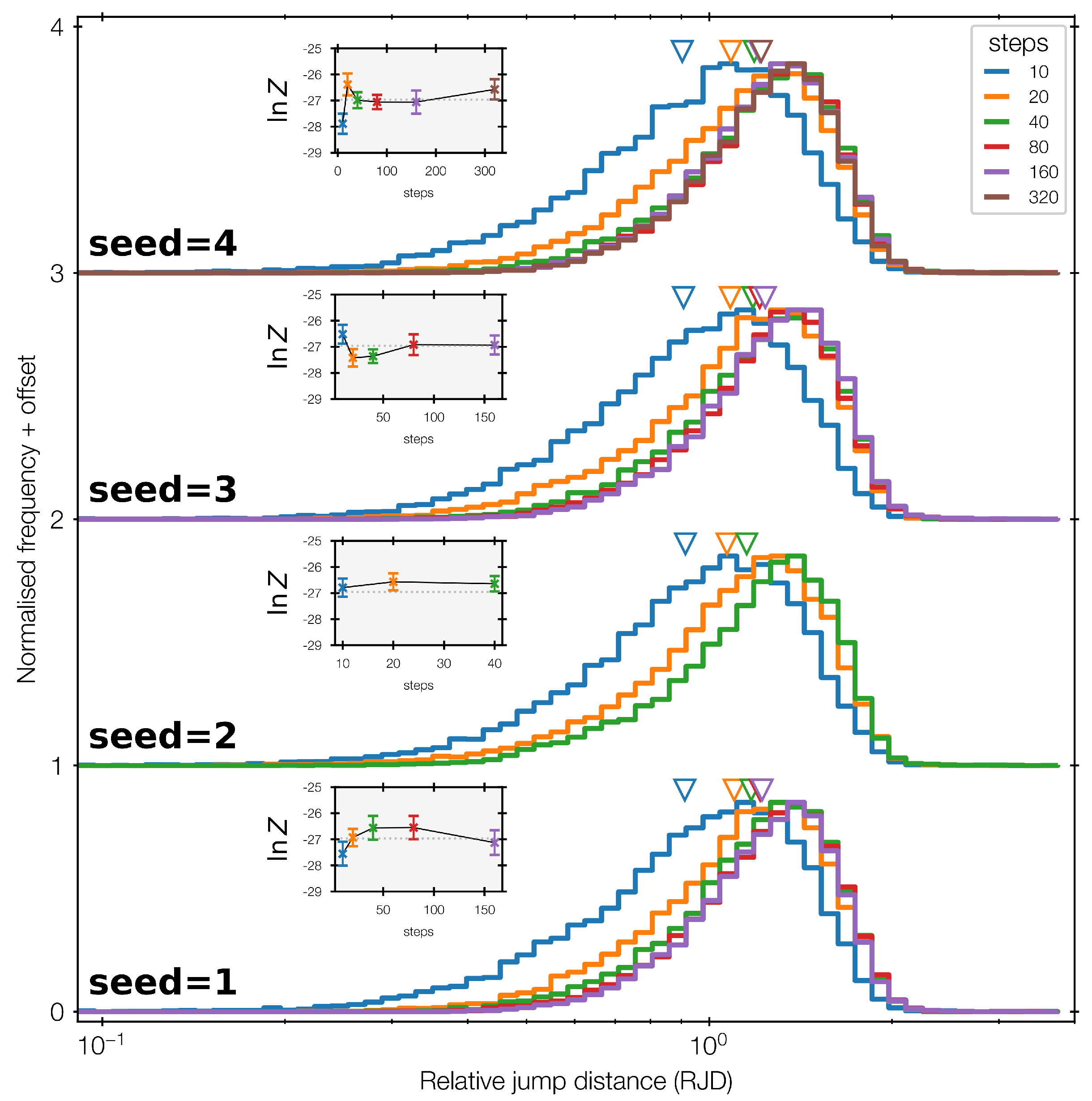
We investigate the diagnostic for sensitivity to Monte Carlo random numbers. Figure 14 shows reruns with different seeds. Comparing the insets across rows in Figure 14, the evidence estimate scatters within the error bar sizes. Because we double the number of steps until the last three lnZ error bars overlap, the scatter in the lnZ estimate changes the final number of steps. This is reflected in the different number of error bars in the insets and different number of histograms for each seed row in Figure 14. Unlike the evidence estimates, the RJD distributions of the same colour appears stable across panels. Consequently, so are the geometric means (downward-pointing triangles).
Figure 14.
Same as Figure 12, but with different random number generator seeds. The number of step doublings until the last three lnZ error bars overlap (see insets) varies. At low number of steps, the evidence estimate scatters within the error bar sizes. The RJD distributions of the same colour across panels, and geometric means (downward-pointing triangles) are stable.
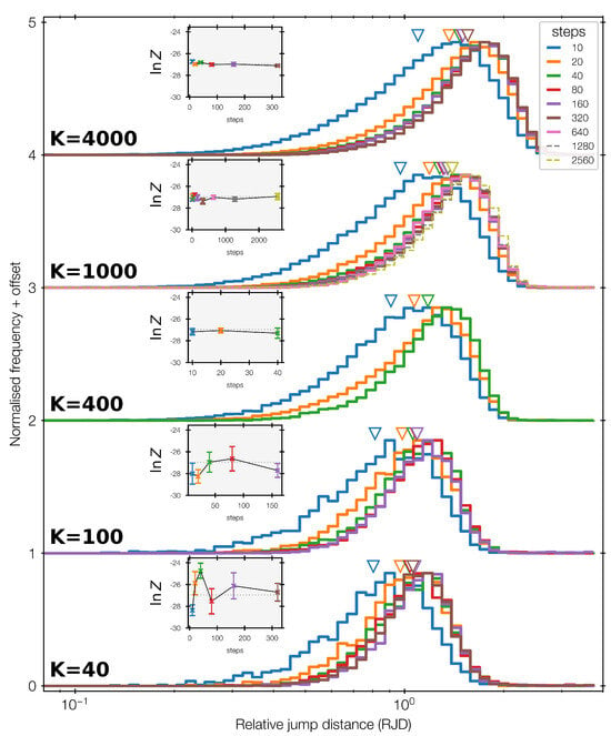
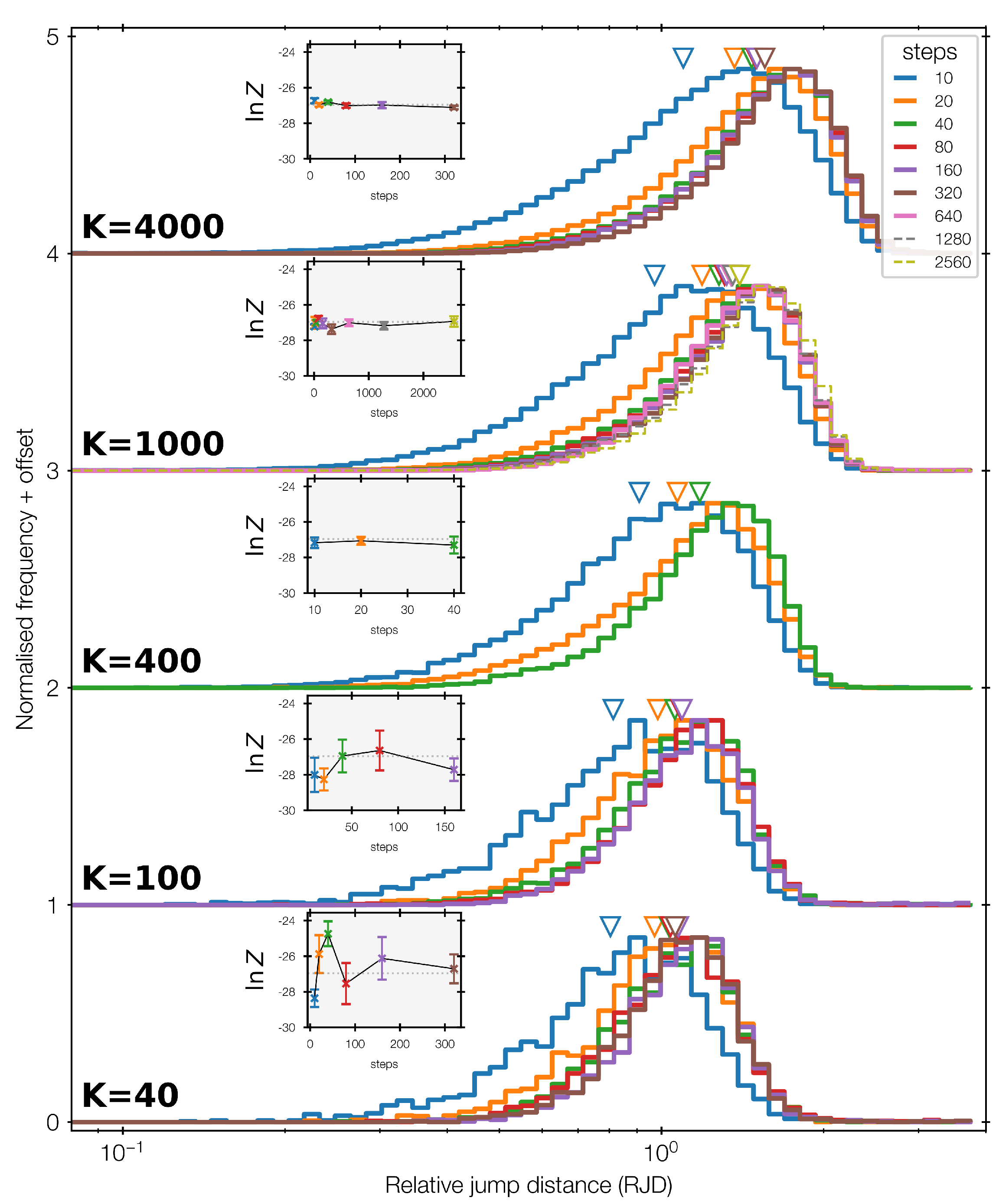
Next, we investigate the behaviour as the number of live points is changed. Figure 15 shows five runs with K = 40 to 4000 as rows. As expected, the evidence estimates (see insets) scatter more at low K (bottom), and overall around the true value (dotted horizontal line). Comparing the blue histogram in Figure 15 from bottom to top rows, the RJD distributions at same number of steps (same colour) move to the right with increasing K. While the slice sampler at the same likelihood threshold has identical behaviour, the spacing of live points, and therefore the reference distance r, and the distance until a live point is sufficiently decorrelated from the starting point decreases. This idea is also exploited in snowballing nested sampling [19], increasing K instead of doubling the number of steps.
Figure 15.
Same as Figure 12, but varying the number of live points K. Evidence estimates (see insets) scatter more at low K (bottom). Comparing the blue histogram from bottom to top rows, the RJD distributions at same number of steps (same colour) move to the right with increasing K.
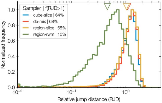
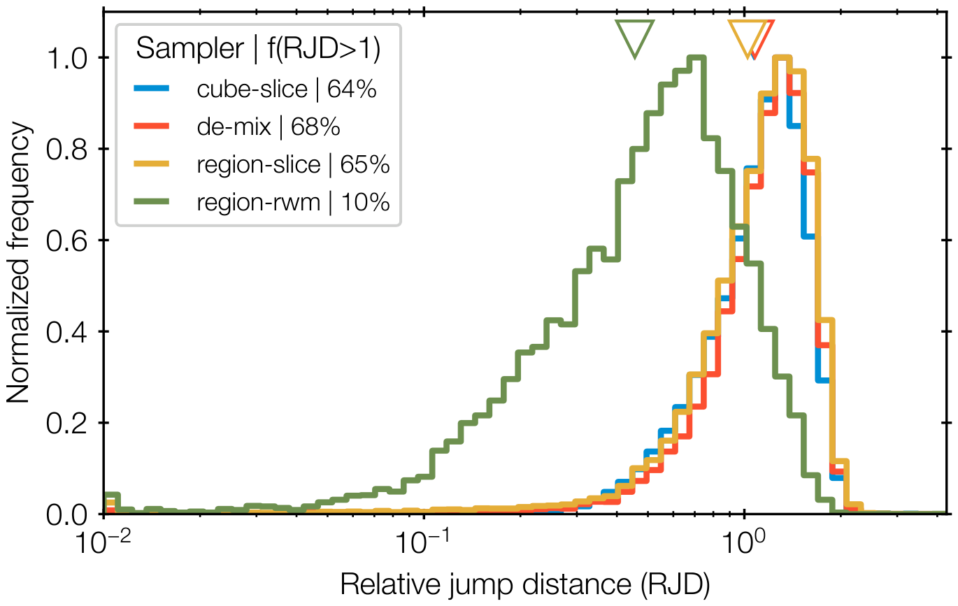
Lastly, we test with the same 10d funnel how the diagnostic changes as the proposal is altered. The results are presented in Figure 16. We adopt slice sampling variants previously analysed in [10]. Besides the hypercube axes-aligned slice sampling (cube-slice) used before, we add the same but proposing along the axis of the empirical covariance of the live points (region-slice). Next, we add the recommended default in ultranest, which randomly chooses proposals between region-slice and selecting a direction from the difference vector of a randomly selected pair of live points (de-mix). All slice sampling variants have M = 20 slice sampling steps with K = 400 live points. The RJD distributions of these different slice samplers (blue, red, yellow curves) are very similar. These runs cost lie between 1 and 2 million model evaluations. We also add an RWM, with a multivariate Gaussian proposal distribution based on empirical live point covariance (region-rwm). The proposed direction sampled is further scaled by a factor, which is, for simplicity, symmetrically multiplied (or divided) on proposal acceptance (rejection) by a small factor . The meaning of the number of steps M differs here. In slice sampling, M refers to the number of slices proposed and navigated, typically requiring O(10) model evaluations. In Random Walk Metropolis, M equals the number of model evaluations. We chose the region-rwm run with M = 160, to obtain a comparable 2 million model evaluations. The typical RJD values of Random Walk Metropolis, green in Figure 16, are lower than for slice sampling, indicating insufficient motion of the live points.
Figure 16.
Same as Figure 12, but varying the sampling proposal, including hypercube axes-aligned slice sampling (cube-slice), live point empirical covariance axes-aligned slice sampling (region-harm), randomly choosing between region-harm and selecting a direction from a random pair of live points (de-mix), Gaussian random walk Metropolis based on empirical live point covariance (region-rwm). The RJD distributions of the different slice samplers (blue, red, yellow curves) are very similar, while the green curve is at lower typical RJD values.
3.7. Eight Schools
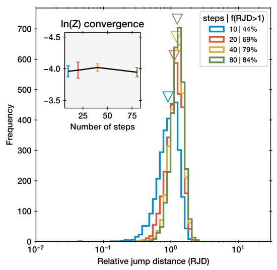
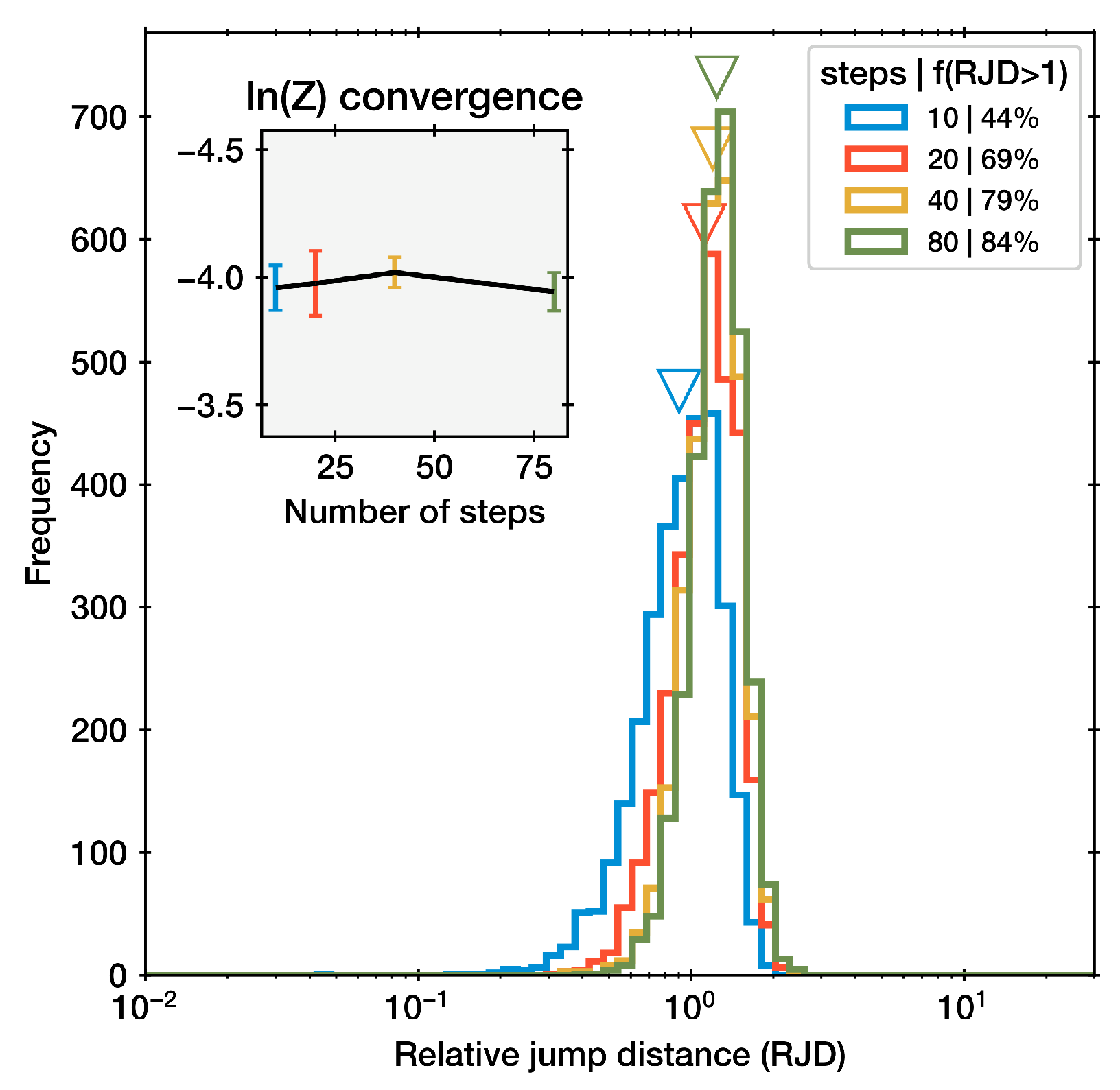
We present a real-world inference problem from [28], which obtained Gaussian measurements from eight schools of a treatment effect: . The mean treatment effect and the variance over all schools is of interest. We therefore define a non-centred parameterization: with the x’s assigned unit Gaussian priors. The hyper-parameters and are assigned a Gaussian and half-Cauchy distribution, respectively, with mean zero and scale 5. The results are presented in Figure 17. They are very similar to the Gaussian and Box toy examples. There is no variation in ln(Z), but a noticeable change in RJD. The geometric mean RJD is 0.9 and 1.24 at the lowest and highest number of steps, respectively. The fraction f(JD > r) rises from 44% to 84%.
Figure 17.
The RJD distributions of the eight schools inference runs. These shift to the right with increasing number of steps. The evidence estimates shown in the inset overlap within the error bars.
3.8. Gravitational Waves
The gravitational wave event GW170817 was observed by the LIGO Hanford, Livingston, and Virgo detectors, and inferred to be a binary neutron star inspiral [29]. We follow the PyCBC tutorial2 and estimate the masses, inclination, distance, chirp time and position on the sky simultaneously with the marginalized phase Gaussian Noise likelihood (see [30]) implemented in [31]. For the sine of the inclination angle, a uniform prior is assumed. The prior for the position is uniform on the sphere. The prior on the distance is assumed to be uniform between 10 and 100 Mpc. The prior on the chirp mass (in solar masses) and mass ratio q is assumed uniform between 1 and 2. The prior on the time of coalescence is assumed uniform between 0.02 and 0.05s of the merger data set time stamp.
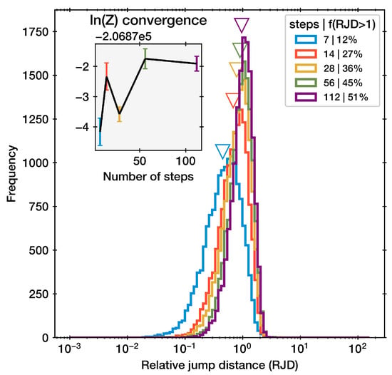
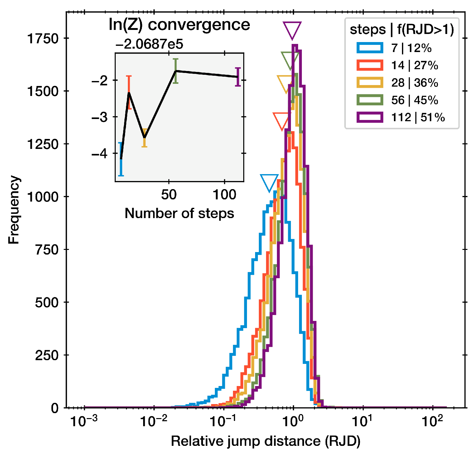
Figure 18 presents the RJD distribution of a sequence of runs. In the run with few steps (7; blue) the geometric mean lies well below 1 and the f(RJD > 1) is very low at 12%. Subsequent doubling of the number of steps increases the fraction up to 50%, with the geometric mean of RJD nearing 1. Runs with even more steps were not computed due to the computational cost.
Figure 18.
The RJD distributions of GW170817 inference runs. These shift to the right with increasing number of steps. The evidence estimates are in the inset. They appear not converged at least with fewer than 56 steps. The chirp mass mchirp is in solar masses, distance in Mpc, chirp time tc in seconds, while ra and dec are in degrees.
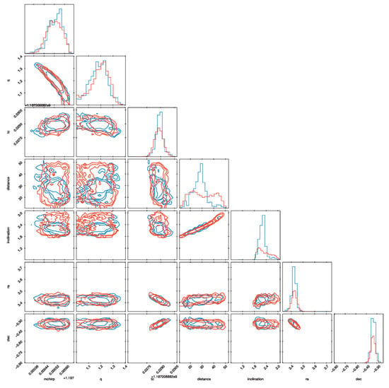
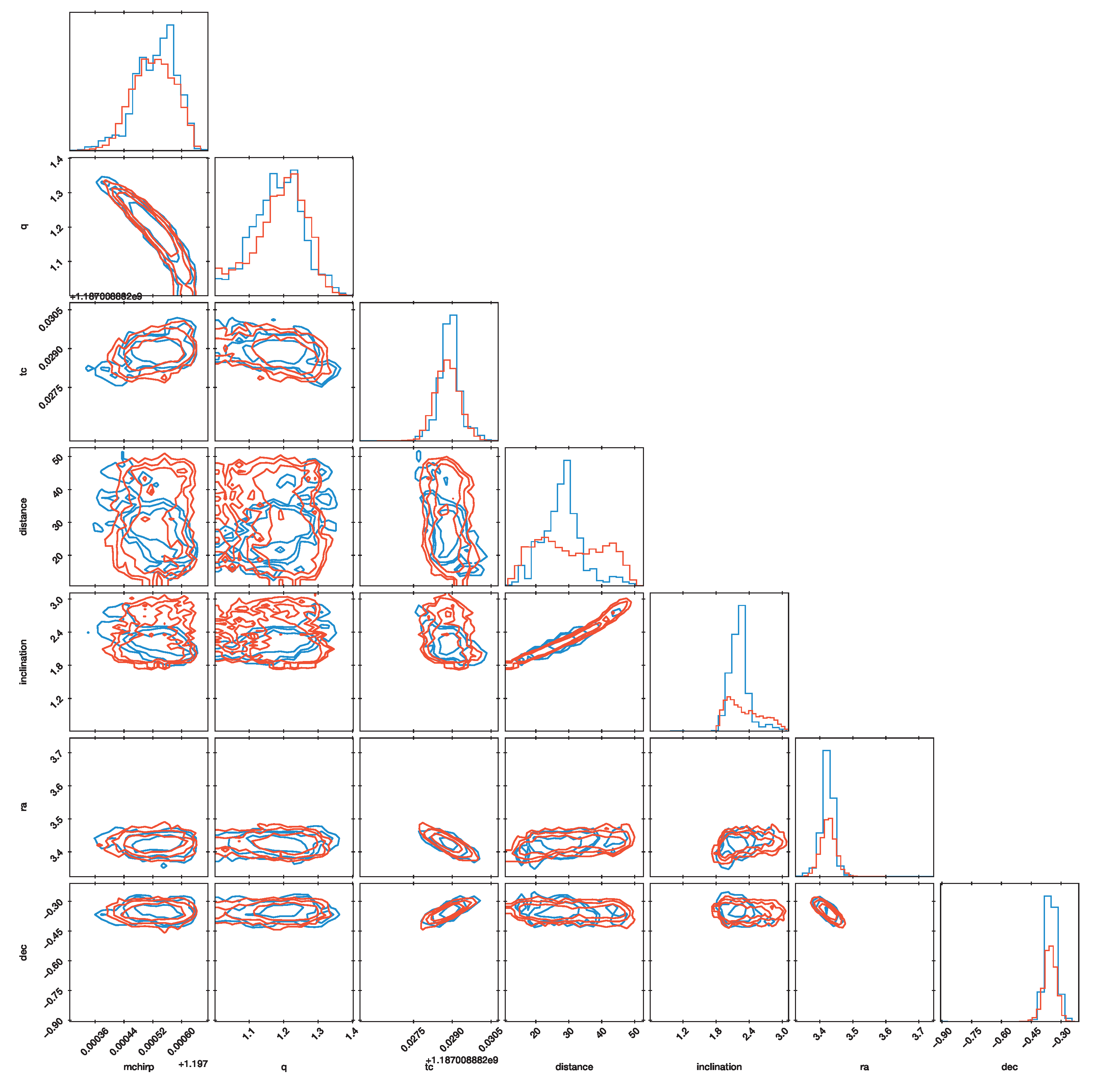
The posterior distribution is presented in Figure 19. The constraints are comparable to those published in [32], with minor differences likely arising due to the different, broader priors adopted here. With a low number of steps (7; blue), the distance posterior is much narrower than with the largest number of steps (112; red). This may be because the degeneracy between inclination, distance and time of coalescence could not be sufficiently explored. This demonstrates that the calibration of the number of steps can have consequences for the astrophysical interpretation of the event.
Figure 19.
Corner plot for GW170817. Red posteriors are from a run with 112 steps, while blue posteriors are from a run with 7 steps. The contours include 39.3%, 86.4% and 95% of the posterior probability distribution. Inclination, RA and Dec are given in units of .
4. Discussion
We introduce a new, widely applicable diagnostic for nested sampling. It is easy to compute for low and high-dimensional inference tasks and does not require multiple nested sampling runs.
4.1. Sensitivity and Reliability
The diagnostic is more sensitive than previously proposed tests. We compared the RJD distribution, the insertion order U-test and ln(Z) convergence on several applications. The relative jump diagnostic is much more sensitive than the insertion order U-test. This is likely related to using more information, namely d-dimensional spatial coordinates rather than likelihood quantiles. Insertion indices discard information on the geometry of the likelihood-restricted prior, so a replacement live point can have an appropriate index while remaining very close to the starting point. For step-based sampling in particular, a short chain started at a random live point can produce a highly correlated replacement, while not leading to the insertion order test failing. This highlights a limitation of the test in the case of step-based samplers. The relative jump diagnostic appears to be at least as sensitive as observing ln(Z). An important difference is that, rather than requiring a sequence of runs, the fraction of RJD > 1 provides a sensitive test of a performed or on-going run in isolation.
This sensitivity arises because the RJD diagnostic directly measures the geometric property, chain diffusion relative to the constrained prior extent, that is most closely linked to the failure mode of interest: a walk that is not sufficiently mixing within the likelihood-restricted prior. The insertion order test [14,15], by contrast, is a one-dimensional test based only on likelihood quantiles, discarding spatial information. It can fail to detect chains that are stuck but happen to produce new points at correct likelihood quantiles, for example, when multiple modes exist at similar likelihoods but the chain cannot traverse between them. The ln(Z) comparison across runs with different step counts is a powerful but expensive global test, sensitive to accumulated errors in the evidence integral. The RJD diagnostic provides a local, iteration-level signal of the same underlying problem, at negligible additional computational cost.
The derivation and validation with toy problems suggest that in mono-modal posteriors the nested sampling run should not be considered trustworthy when f(JD < r) is below 50 per cent, and the geometric mean of RJD is below 1. Intuitively, the former criterion says that the median jump distance is below the typical distance between live points.
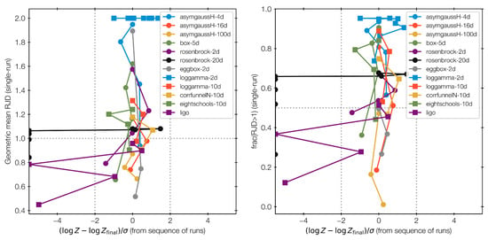
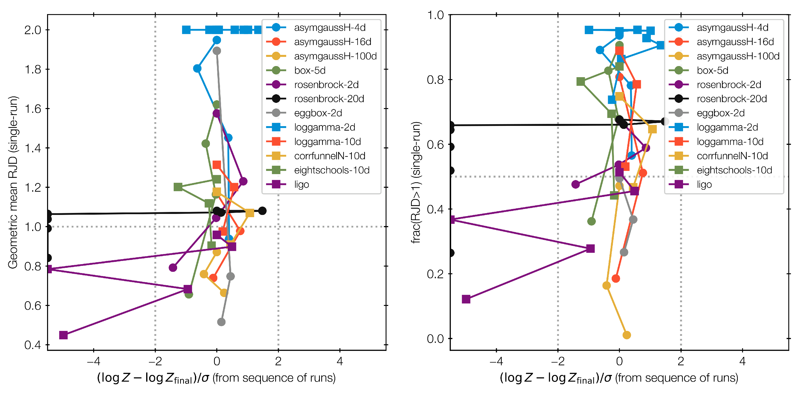
Although our sample of twelve inference problems in 2 to 100 dimensions is limited, we can attempt to understand the false positive and negative rates of these criteria. Figure 20 presents all runs performed (see Appendix B for a table of values). The lines connect nested sampling runs on identical problems as the number of steps is doubled, which we term a ladder here. Considering each ladder of runs, the closer the evidence estimate to the reference evidence, the higher the diagnostics. We observe Spearman in 12 of 12 cases with a median of −0.50. Figure 20 plots the relative error in log-evidence is plotted against the two new diagnostic criteria. In this case, we consider two sigma deviations from the true evidence value, or if not available, from the evidence value derived in the highest M run, problematic. The relative error is capped at 5.5. These limits are indicated as vertical dotted lines. The horizontal dotted line uses our criteria to identify problematic runs (bottom half) from acceptable runs (top half). With these nominal thresholds motivated by theory, the criteria are hardly better than chance in their false positive and false negative rates (30–50%), most notably rosenbrock-20d. However, with thresholds of geometric mean RJD > 1.1, there are 0 (out of 9) false positives with a false negative rate of 44% (19/43). With frac(RJD > 1) > 70%, the false positive rate is also 0% (0/9) with a false negative rate of 56% (24/43). Those criteria are therefore primarily useful to vouch for runs, but failing the criterion does not necessarily imply a bad result. A caveat here is that for the most realistic problems the true evidence value is unknown, and proper calibration of thresholds would need a larger sample with a hold-out set.
Figure 20.
Collection of all runs, in the relative log-evidence error compared to the geometric mean RJD (left) and the fraction of RJD > 1. Vertical dotted lines indicate 2 deviation range. The horizontal dotted line indicates a geometric mean RJD of unity (left panel) and (right panel), respectively.
The expected relative jump distance can be over-estimated. If the number of live points is low and/or the dimensionality high, clusters and local structures may be unrecognizable when computing the typical neighbour distance. Similarly, if the reference distance is only computed every nth iteration, the moment when a likelihood-restricted prior becomes multi-modal and modes can no longer be traversed may be missed. At that moment, r may reflect the spacing across the full multi-modal distribution rather than within a single mode, causing r to be over-estimated and RJD to appear deceptively low even when the walk is mixing well within each mode. We observe such behaviour with the multi-modal Eggbox and Loggamma toy problems.
Based on our results, we preliminarily recommend the following procedure for practitioners: (1) If the geometric mean RJD is above 1.1, then the nested sampling result might be trustworthy. (2) Otherwise, rerun with twice as many steps. If either the RJD distribution changed, or the Z estimate changed significantly, go to (1). Otherwise, the result may be acceptable. The cautious practitioner should double the number of steps once more than seems necessary. The major computational benefit of this procedure is that any alteration of the Bayesian model does not automatically incur a re-calibration of the number of steps.
4.2. Future Work
In this work, we have primarily focused on the reliability of evidence estimates, as commonly used for Bayesian model comparison. The effect on the posterior distribution may be different, as previously discussed for MultiNest reliability by [33]. Nevertheless, Figure 19 shows an example where posterior distributions are incorrectly estimated by one run and the criteria flags it as unreliable.
The RJD diagnostic compares the new-born live point to the starting point of its random walk. This makes it specific to step sampling-based nested samplers. A generalization would be to consider the distance of the new-born point to its nearest existing live point, rather than the starting point. Such a generalization could be implemented without modification to existing nested samplers. Our diagnostic is a stronger form, because it uses the most correlated point. Implementation in existing nested sampling packages is easy and demands little additional resources, since only the distance between starting and final point needs to be stored. The RJD diagnostic is implemented in UltraNest3 from version 4.1.
Future work will explore ways to adapt the number of steps during a nested sampling run. Preliminary implementations in UltraNest are available which increase the number of steps after each iteration where RJD < 1, and decrease it after each iteration where RJD > 1. An alternative approach would be to use Snowballing nested sampling [19], i.e., choose a fixed number of steps and bulk up the number of live points in likelihood ranges where f(JD > r) was low. As the density of live points increases, the typical neighbour distance r decreases, which increases RJD without the need to discard existing chains.
Funding
This research received no external funding.
Data Availability Statement
The code for generating the data is available at https://github.com/JohannesBuchner/paper-relative-jump-distance (accessed on 16 October 2026).
Acknowledgments
I thank the two anonymous reviewers and the academic editor for comments and suggestions that improved the manuscript. I thank Will Handley for insightful conversations, which were hosted by the Kavli Institute for Cosmology in Cambridge, UK. AI (primarily Anthropic Claude 4.6) was used for improving the grammar and isolated components of the data analysis.
Conflicts of Interest
The author declares no conflicts of interest.
Appendix A. Reference Distance for Ellipsoids
To illustrate the behaviour of the defined reference distance, we can consider ellipsoidal contours. If we consider that an ellipsoid volume V that is segmented into K equal sub-volumes with a volume proportional to , then . For fixed V, we find the scale between neighbours r scales as .
Figure A1.
Scaling of reference radius with number of live points and dimensionality. Each error bar summarizes the mean and standard deviation from 40 simulations. The dashed curves is Equation (A1). This approximates most data points, but there are deviations in high dimensions and low number of live points.
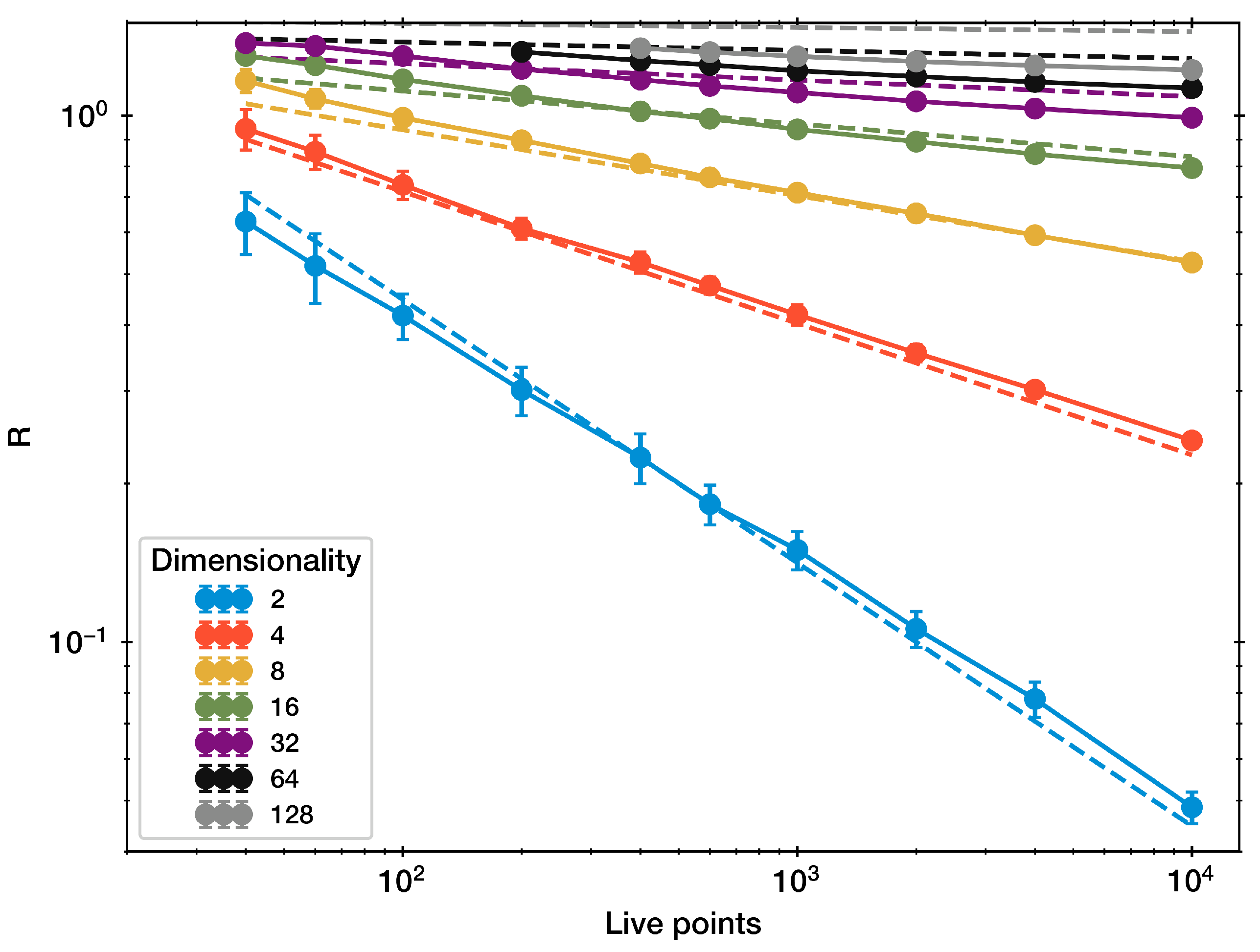
We perform numerical experimentation sampling K points from an ellipsoid in up to 128 dimensions. We compute r with the code listed in Figure A2. The found r values are presented in Figure A1. We also plot the relation
As discussed above, the first term is the volumetric distribution by the K live point in a d-dimensional hyper-sphere. The weak second term is likely related to the empirical whitening transformation failing to accurately identify the true whitening transform in high dimensions.
Figure A2.
Python code to compute MLFriends radius. Function compute_radius is called with an array of live points. The last line takes the square root.
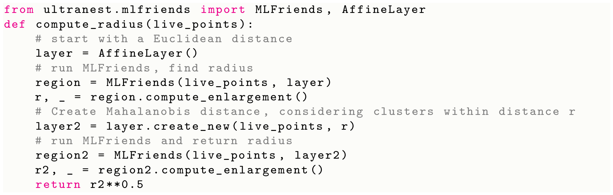
In high dimensions, we find that r lies between 1.2 and 1.3, independent of the number of live points. Likely, this is related to the number of bootstrapping rounds. intuitively corresponds to the Mahalanobis distance of any ellipsoid axis. If we were to adopt , the RJD criterion would become more optimistic about the achieved jump length. In more realistic settings than the ellipsoidal contours considered here, r may be substantially different.
Appendix B. Listing of Inference Runs
Table A1.
Summary of runs: name, dimensionality (d), number of live points (), number of steps, geometric mean RJD, fraction with RJD , evidence estimate , and true value (if available). Bold geometric mean RJD indicates <1; bold indicates <0.5. All listed here are run with K = 400 and the unit-slice proposal.
Table A2.
Summary of runs, continued, for the funnel with d = 10 (corrfunnelN-10d), highlighting changes with different seeds. Bold geometric mean RJD indicates <1; bold indicates <0.5.
Table A3.
Summary of runs, continued, for the funnel with d = 10 (corrfunnelN-10d). Bold geometric mean RJD indicates <1; bold indicates <0.5.
Notes
| 1 | |
| 2 | Tutorial 0 from https://github.com/gwastro/PyCBC-Tutorials/ (version d852bdb2b from 30 July 2024). |
| 3 | https://johannesbuchner.github.io/UltraNest/ (accessed on 20 October 2026). |
References
- Skilling, J. Nested sampling. AIP Conf. Proc. 2004, 735, 395. [Google Scholar] [CrossRef] [Scilit]
- Ashton, G.; Bernstein, N.; Buchner, J.; Chen, X.; Csányi, G.; Fowlie, A.; Feroz, F.; Griffiths, M.; Handley, W.; Habeck, M.; et al. Nested sampling for physical scientists. Nat. Rev. Methods Prim. 2022, 2, 39, Correction in Nat. Rev. Methods Prim. 2022, 2, 44. https://doi.org/10.1038/s43586-022-00138-2. [Google Scholar] [CrossRef] [Scilit]
- Feroz, F.; Hobson, M.P.; Bridges, M. MULTINEST: An efficient and robust Bayesian inference tool for cosmology and particle physics. Mon. Not. R. Astron. Soc. 2009, 398, 1601–1614. [Google Scholar] [CrossRef] [Scilit]
- Handley, W.J.; Hobson, M.P.; Lasenby, A.N. POLYCHORD: Next-generation nested sampling. Mon. Not. R. Astron. Soc. 2015, 453, 4384–4398. [Google Scholar] [CrossRef] [Scilit]
- Speagle, J.S. DYNESTY: A dynamic nested sampling package for estimating Bayesian posteriors and evidences. Mon. Not. R. Astron. Soc. 2020, 493, 3132–3158. [Google Scholar] [CrossRef] [Scilit]
- Buchner, J. UltraNest—A robust, general purpose Bayesian inference engine. J. Open Source Softw. 2021, 6, 3001. [Google Scholar] [CrossRef] [Scilit]
- Higson, E.; Handley, W.; Hobson, M.; Lasenby, A. NESTCHECK: Diagnostic tests for nested sampling calculations. Mon. Not. R. Astron. Soc. 2019, 483, 2044–2056. [Google Scholar] [CrossRef] [Scilit]
- Neal, R.M. Slice sampling. Ann. Stat. 2003, 31, 705–767. [Google Scholar] [CrossRef] [Scilit]
- Jasa, T.; Xiang, N. Using Nested Sampling in the Analysis of Multi-Rate Sound Energy Decay in Acoustically Coupled Rooms. In Proceedings of the AIP Conference Proceedings; American Institute of Physics: College Park, MD, USA, 2005; Volume 803, pp. 189–196. [Google Scholar]
- Buchner, J. Comparison of Step Samplers for Nested Sampling. Proc. Phys. Sci. Forum 2022, 5, 46. [Google Scholar] [CrossRef] [Scilit]
- Salomone, R.; South, L.F.; Drovandi, C.C.; Kroese, D.P. Unbiased and Consistent Nested Sampling via Sequential Monte Carlo. arXiv 2018, arXiv:1805.03924. Available online: https://academic.oup.com/jrsssb/article/87/4/1221/8129577 (accessed on 20 October 2026).
- Buchner, J. A statistical test for Nested Sampling algorithms. Stat. Comput. 2016, 26, 383–392. [Google Scholar] [CrossRef] [Scilit]
- Feroz, F.; Hobson, M.P.; Cameron, E.; Pettitt, A.N. Importance Nested Sampling and the MultiNest Algorithm. Open J. Astrophys. 2019, 2, 10. [Google Scholar] [CrossRef] [Scilit]
- Fowlie, A.; Handley, W.; Su, L. Nested sampling cross-checks using order statistics. arXiv 2020, arXiv:2006.03371. [Google Scholar] [CrossRef] [Scilit]
- Buchner, J. Nested sampling methods. Stat. Surv. 2023, 17, 169–215. [Google Scholar] [CrossRef] [Scilit]
- Higson, E.; Handley, W.; Hobson, M.; Lasenby, A. Dynamic nested sampling: An improved algorithm for parameter estimation and evidence calculation. arXiv 2017, arXiv:1704.03459. Available online: https://link.springer.com/article/10.1007/s11222-018-9844-0 (accessed on 20 October 2026).
- Chopin, N.; Robert, C.P. Properties of nested sampling. Biometrika 2010, 97, 741–755. [Google Scholar] [CrossRef] [Scilit]
- Nelson, B.E.; Ford, E.B.; Buchner, J.; Cloutier, R.; Díaz, R.F.; Faria, J.P.; Hara, N.C.; Rajpaul, V.M.; Rukdee, S. Quantifying the Bayesian Evidence for a Planet in Radial Velocity Data. Astron. J. 2020, 159, 73. [Google Scholar] [CrossRef] [Scilit]
- Buchner, J. Snowballing Nested Sampling. Phys. Sci. Forum 2023, 9, 17. [Google Scholar] [CrossRef] [Scilit]
- Pasarica, C.; Gelman, A. Adaptively scaling the Metropolis algorithm using expected squared jumped distance. Stat. Sin. 2010, 20, 343–364. [Google Scholar]
- Handley, W.J.; Hobson, M.P.; Lasenby, A.N. POLYCHORD: Nested sampling for cosmology. Mon. Not. R. Astron. Soc. 2015, 450, L61–L65. [Google Scholar] [CrossRef] [Scilit]
- Buchner, J.; Georgakakis, A.; Nandra, K.; Hsu, L.; Rangel, C.; Brightman, M.; Merloni, A.; Salvato, M.; Donley, J.; Kocevski, D. X-ray spectral modelling of the AGN obscuring region in the CDFS: Bayesian model selection and catalogue. Astron. Astrophys. 2014, 564, A125. [Google Scholar] [CrossRef] [Scilit]
- Buchner, J. First analytical coverage bounds of a fully specified nested sampling algorithm. arXiv 2026, arXiv:2606.22930. [Google Scholar] [CrossRef] [Scilit]
- Francois, D.; Wertz, V.; Verleysen, M. The Concentration of Fractional Distances. IEEE Trans. Knowl. Data Eng. 2007, 19, 873–886. [Google Scholar] [CrossRef] [Scilit]
- Feroz, F.; Hobson, M.P. Multimodal nested sampling: An efficient and robust alternative to Markov Chain Monte Carlo methods for astronomical data analyses. Mon. Not. R. Astron. Soc. 2008, 384, 449–463. [Google Scholar] [CrossRef] [Scilit]
- Beaujean, F.; Caldwell, A. Initializing adaptive importance sampling with Markov chains. arXiv 2013, arXiv:1304.7808. [Google Scholar] [CrossRef] [Scilit]
- Karamanis, M.; Beutler, F. Ensemble Slice Sampling. arXiv 2020, arXiv:2002.06212. [Google Scholar] [CrossRef] [Scilit]
- Rubin, D.B. Estimation in parallel randomized experiments. J. Educ. Stat. 1981, 6, 377–401. [Google Scholar] [CrossRef] [Scilit]
- Abbott, B.P.; Abbott, R.; Abbott, T.D.; Acernese, F.; Ackley, K.; Adams, C.; Adams, T.; Addesso, P.; Adhikari, R.X.; Adya, V.B.; et al. GW170817: Observation of Gravitational Waves from a Binary Neutron Star Inspiral. Phys. Rev. Lett. 2017, 119, 161101. [Google Scholar] [CrossRef] [Scilit] [PubMed]
- Biwer, C.M.; Capano, C.D.; De, S.; Cabero, M.; Brown, D.A.; Nitz, A.H.; Raymond, V. PyCBC Inference: A Python-based Parameter Estimation Toolkit for Compact Binary Coalescence Signal. Publ. Astron. Soc. Pac. 2019, 131, 024503. [Google Scholar] [CrossRef] [Scilit]
- Nitz, A.; Harry, I.; Brown, D.; Biwer, C.M.; Willis, J.; Canton, T.D.; Capano, C.; Dent, T.; Pekowsky, L.; Davies, G.S.C.; et al. gwastro/pycbc: v2.3.3 Release of PyCBC, version v2.3.3. Computer Software. Zenodo: Geneva, Switzerland, 2024. [CrossRef]
- Finstad, D.; De, S.; Brown, D.A.; Berger, E.; Biwer, C.M. Measuring the Viewing Angle of GW170817 with Electromagnetic and Gravitational Waves. Astrophys. J. Lett. 2018, 860, L2. [Google Scholar] [CrossRef] [Scilit]
- Dittmann, A. Notes on the Practical Application of Nested Sampling: MultiNest, (Non)convergence, and Rectification. Open J. Astrophys. 2024, 7, 79. [Google Scholar] [CrossRef] [Scilit]
Disclaimer/Publisher’s Note: The statements, opinions and data contained in all publications are solely those of the individual author(s) and contributor(s) and not of MDPI and/or the editor(s). MDPI and/or the editor(s) disclaim responsibility for any injury to people or property resulting from any ideas, methods, instructions or products referred to in the content. |
© 2026 by the author. Licensee MDPI, Basel, Switzerland. This article is an open access article distributed under the terms and conditions of the Creative Commons Attribution (CC BY) license.