Representations of the Schwarzschild Geometry: From Classical Coordinates to the Golden Minisuperspace

Abstract

We derive and present visual and geometric representations of the Schwarzschild metric. The analysis spans classical (tortoise, Kruskal) and compact pulsating (diamond) coordinates. Building upon a reduced radial minisuperspace formulation of Schwarzschild dynamics—wherein a Fibonacci matrix naturally yields golden-ratio eigenvalues—we introduce the golden representation and its complex spiral mapping. While the underlying reduced Lagrangian and radial minisuperspace metric are known in the literature, we demonstrate how this flat configuration space provides a useful visual tool for disentangling physical observables. Specifically, we show that the local gravitational redshift, the areal radius and the logarithmic excess in radial Schwarzschild coordinate travel time are mapped onto orthogonal coordinate projections and complex polar components within the radial minisuperspace geometry.

1. Introduction

Immediately after Einstein presented the field equations of General Relativity (GR) in 1915, Schwarzschild obtained the first exact solution to them: the spacetime outside a spherical and non-rotating object. It allowed for the description, to a good approximation, of the geometry outside astrophysical objects like planets and stars. It was also the prelude for describing the simplest black hole [1]. In the following decades, alternative descriptions of it were discovered and analyzed, while parallel developments in the realm of cosmology were made [2,3]. In black hole theory and cosmology, it became mandatory to explore the subtleties related to the covariance of GR, the equivalence principle, and the meaning of specific coordinate descriptions in analytic solutions [4,5,6,7,8,9,10]. The issue of coordinates and representations continues to be a relevant topic on both fronts [11,12,13,14].

In this article, we analyze different representations of the Schwarzschild spacetime. We start by recalling simple properties that can be extracted from Schwarzschild coordinates. Then, we present some classical representations, such as the near-horizon approximation, the embedding of spatial sections, and the tortoise and Kruskal coordinates. We also present two novel representations. First, we present the diamond representation, recently introduced as an extension of a unified scheme for obtaining the tortoise and Kruskal coordinates [15]. Second, the golden representation is introduced here, building on previous work highlighting the dimensional reduction in the form of a radial minisuperspace (an auxiliary configuration space), as well as the appearance of the golden ratio in black-hole solutions [16,17,18,19,20,21,22,23].

Several developments have recently occurred in this field, but here, we clarify some issues that allow us to contrast and relate these representations. For instance, the pulsating coordinates underlying the diamond representation were introduced recently, and motivated the recent proposal (causal diamond coordinates) for the Minkowski spacetime in Refs. [12,24]. Here, we clarify some issues related to the invertibility and the role of the diamond boundary of the representation.

In a similar vein, the reduced action for static spherically symmetric gravity and its minisuperspace Hamiltonian structure have a rich history [16,17]. The reduced variables $(q^1,q^2)$, the matrix $Q_{ab}$, its golden-ratio eigenvalues, and its reduction to static Schwarzschild solutions were developed in Ref. [20]. Furthermore, Christodoulakis et al. (building on Cavaglià et al.) analyzed the underlying reduced Lagrangian and demonstrated that its three Killing vectors form the $ISO(1,1)$ Poincaré algebra, implicitly establishing the flatness of the minisuperspace metric [17,18,19]. The inclusion of charged black holes was also considered in this framework, in Refs. [21,22]. In the present work, after deriving these foundational reduced field equations in simple and illustrative terms, we also construct a unified visual and physical synthesis across these representations. Specifically, we introduce novel graphical mappings—most notably the complex golden spiral—and demonstrate how key physical observables (such as the gravitational redshift factor, the areal radius, and the radial coordinate travel time excess) can be directly read off as linear and polar geometric features in a flat configuration space. In the process, as we argue in the final part of this work, some interesting relationships arise between distinct representations.

The rest of this article is structured as follows: In Section 2, we present the Schwarzschild solution and briefly review some direct features that can be extracted from it. Then, we obtain the near-horizon approximation alongside its connection with accelerated frames and the Flamm representation. Section 3 presents a derivation of the tortoise and the Kruskal representations using the same procedure. Then, we show the diamond representation, which shares a common feature with the former two: they are all (1+1)-conformally flat to hypersurfaces of the Schwarzschild spacetime at constant angles. In Section 4, we introduce the golden representation by slightly deforming the customary Schwarzschild ansatz and dimensionally reducing the Einstein–Hilbert action, until the golden coordinates are defined. In Section 5, we show how the geodesics of the (1+1)-dimensional auxiliary configuration space reproduce the geometry upon fixing the radial gauge and selecting appropriate integration constants. This, in turn, motivates us to present different visual golden representations of the Schwarzschild geometry in Section 6. We end with a summary of our work and some final comments in Section 7. In Appendix A, we present some properties of the golden ratio and of a specific radial coordinate value—which we term the golden radius—identifying it as a distinguished point of our chosen graphical parametrization, and relate it to the different representations.

2. Near-Horizon Approximation and the Flamm Parabola

Many analytic solutions to Einstein’s field equations, namely

$$R_{\mu \nu }-{\displaystyle \frac{1}{2}}{g}_{\mu \nu }R=8\pi T_{\mu \nu },$$

(1)

take the spherically symmetric form [1,25]

$$d{s}^2=-e^{2\alpha \left(r\right)}d{t}^2+e^{2\beta \left(r\right)}d{r}^2+r^{2}d{\mathrm{\Omega }}^2,$$

(2)

where $d{\mathrm{\Omega }}^2=d{\theta }^2+{\sin }^2\theta d{\varphi }^2$. We use units where $c=G=1$ and Greek indices like $\mu ,\nu$ run from 0 to 3. Many of the solutions share the property $\beta =-\alpha$ [26,27,28,29]. The interpretation of a cosmological or black hole origin of the solutions may be subtle. For instance, if the energy-momentum tensor comes from a constant energy density filling an isotropic and homogeneous space, the de Sitter or two Lanczos universes can take the same static form. But having distinct spatial curvature, they take a specific FLRW form in the comoving frame [29]. In a similar vein, assuming a central spherical source can lead to either the Schwarzschild–de Sitter or the Schwarzschild solution [3]. The latter is the simplest of all, where $T_{\mu \nu }=0$ in (1) outside a certain radius, implying $R=0$. Einstein’s equations reduce to $R_{\mu \nu }=0$, and the metric solution is

$$d{s}^2=-\left(1-{\displaystyle \frac{r_s}{r}}\right)d{t}^2+{\displaystyle \frac{d{r}^2}{1-\frac{r_s}{r}}}+r^{2}d{\mathrm{\Omega }}^2,$$

(3)

where $r_s$ is the Schwarzschild radius. This is an appropriate solution outside massive spherical objects, when their angular momentum can be neglected.

A distant observer observes a time dilation for an event at r given by $dt={\left(-g_{00}\right)}^{-1/2}d\tau$. Then, when a photon travels along a radial geodesic from a given r, a faraway observer measures it gravitationally redshifted by ${\omega }^{\prime }={\omega }_0\sqrt{-g_{00}}={\omega }_0\sqrt{1-r_s/r}$. We shall refer to $\sqrt{1-r_s/r}$ as the redshift factor [25]. Also, one has the relation

$$dr=d\varrho \sqrt{1-{\displaystyle \frac{r_s}{r}}},$$

(4)

which is a geometric relation between the areal-radius differential and the proper radial distance $d\varrho$ on a static spatial slice. The coordinate t represents the proper time recorded by a static observer at spatial infinity, and r is the geometrically defined areal radius. One can approximate the geometry just above $r_s$ as follows. Since $d\varrho$ in (4) represents the proper radial infinitesimal distance at a fixed r, we can integrate it as

$$\varrho =\sqrt{r\left(r-r_s\right)}+r_s{\sinh }^{-1}\sqrt{r/r_s-1}.$$

(5)

Since ${\sinh }^{-1}z\approx z$ for $z\ll 1$, Equation (5) yields an approximation for $r\cong r_s$ as [29]

$$r=r_s+{\displaystyle \frac{{\varrho }^2}{4r_s}}.$$

(6)

Also, since $\varrho \ll 2r_s$, then $1-r_s/r={\varrho }^2/\left({\varrho }^2+4r_s^2\right)\approx {\varrho }^2/\left(4r_s^2\right)$. Rescaling the time as $t=2r_{s}T$ and using $\varrho =\zeta$ for the approximated variable, the first two terms in Equation (3) become $-{\zeta }^{2}d{T}^2+d{\zeta }^2$. Consider very small variations in the angle $\theta$ with respect to the (arbitrary) z-direction. Then, $x\cong r_s\theta \cos \varphi$ and $y\cong r_s\theta \sin \varphi$. Thus, $r_s^2(d{\theta }^2+{\theta }^{2}d{\varphi }^2)=d{x}^2+d{y}^2$ can be substituted into the last terms of Equation (3), resulting in the following [30]:

$$d{s}^2=-{\zeta }^{2}d{T}^2+d{\zeta }^2+d{x}^2+d{y}^2.$$

(7)

This approximates Minkowski spacetime, given the Rindler transformations $t=\zeta \sinh T$ and $z=\zeta \cosh T$. The sections of hyperbolas induced by $z^2-t^2={\zeta }^2$ for $\zeta =const.$ are timelike trajectories with acceleration $a={\zeta }^{-1}$. Because Equation (6) implies that $\zeta \to 0$ as $r\to r_s$, there is a direct association between the Rindler horizon for a highly accelerated (flat) frame in a radial direction and the Schwarzschild (curved) event horizon [31,32].

Embedding diagram. By setting $dt=0$ and $\theta =\pi /2$ in Equation (3), we obtain the reduced metric ${(1-{\displaystyle \frac{r_s}{r}})}^{-1}d{r}^2+r^{2}d{\varphi }^2$, which can be embedded into the target Euclidean space as follows:

$$d{\sum }^2=d{\rho }^2+{\rho }^{2}d{\varphi }^2+d{z}^2,$$

(8)

where $(\rho ,\varphi ,z)$ are cylindrical coordinates. By identifying the azimuthal angles, one has $\rho =r$. The two-dimensional surface induces the dependence $dz=\sqrt{1/(r/r_s-1)}dr$, which can be integrated to yield $z=\sqrt{4r_s\left(r-r_s\right)}$, or equivalently

$$r={\displaystyle \frac{z^2}{4r_s}}+r_s.$$

(9)

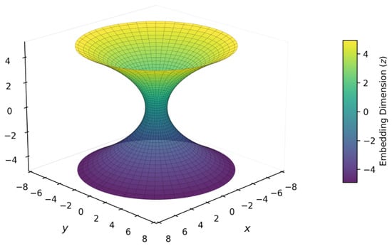
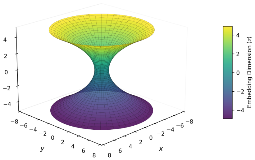
By allowing negative values of z and recalling the azimuthal symmetry in Equation (8), the familiar Flamm paraboloid is obtained (Figure 1) [1,33]. This diagram can be associated with two copies of the same spacetime, or with two disjoint spacetimes, with the circle in $z=0$ acting as the throat of a wormhole connecting them. This embedding makes visually explicit that traveling along the parabola on a radial path covers more distance than the straight-line Euclidean distance $d\rho$. Given the construction made, Measuring the radial path along this parabola is equivalent to integrating the proper radial distance in (4) [34].

Figure 1. Flamm paraboloid. Spatial embedding of the Schwarzschild geometry.

That is, Figure 1 illustrates the proper radial distance along a Schwarzschild-time slice. Finally, Equations (6) and (9) have the same dependence on r: under the near-horizon approximation, the proper radial distance $\varrho$ associated with Rindler is well approximated by the value z in the Flamm paraboloid.

3. Kruskal and Pulsating Transformations

By setting $d\theta =d\varphi =0$ and $d{s}^2=0$ in Equation (3), the local light-cone structure for $r>r_s$ is explicitly revealed in $(t,r)$-coordinates in the form

$${\displaystyle \frac{dt}{dr}}=\pm {\displaystyle \frac{1}{1-\frac{r_s}{r}}}.$$

(10)

In a $t-r$ diagram, the light cones become highly tilted for r just above the horizon. The tortoise representation recovers the $\pm 1$ slope [25,35].

We begin by expressing the first two terms on the right-hand side of Equation (3) as $-\gamma d{t}^2+{\gamma }^{-1}d{r}^2={\omega }^2(-d{T}^2+d{R}^2)$, where $\gamma =1-r_s/r$ and ${\omega }^2$ is the conformal factor. Now, consider the metric transformation $g_{ab}=g_{a^{\prime }{b}^{\prime }}{\partial }_a{x}^{a^{\prime }}{\partial }_b{x}^{b^{\prime }}$, where the indices a and b are 0 or 1, and the primed indices refer to the metric with ${\omega }^2$. Considering the 00, 11 and 01 components of the transformation, and after rearranging terms, one obtains

$${\left({\partial }_{t}T\right)}^2={\left({\partial }_{t}R\right)}^2+{\omega }^{-2}\gamma ,$$

(11)

$${\left({\partial }_{r}T\right)}^2={\left({\partial }_{r}R\right)}^2-{\omega }^{-2}{\gamma }^{-1}$$

(12)

and

$${\left({\partial }_{t}T\right)}^2{\left({\partial }_{r}T\right)}^2={\left({\partial }_{t}R\right)}^2{\left({\partial }_{r}R\right)}^2.$$

(13)

Inserting Equations (11) and (12) into (13) and simplifying yields ${\omega }^{-2}=\gamma {\left({\partial }_{r}R\right)}^2-{\gamma }^{-1}{\left({\partial }_{t}R\right)}^2$. We can substitute this back into Equation (11) to obtain the simplified form

$${\partial }_{t}T=\gamma {\partial }_{r}R.$$

(14)

Now, we assume that $T=T\left(t\right)$ and $R=R\left(r\right)$. For this case, Equation (14) must equal a constant. One may choose $T=t$ in Equation (14), while $\gamma =1-r_s/r$ leads to

$$R=r^{\ast }:=\int {\gamma }^{-1}dr=r+r_s\ln \left({\displaystyle \frac{r}{r_s}}-1\right).$$

(15)

The conformal factor then becomes ${\omega }^{-2}=\gamma {\left(dR/dr\right)}^2={\gamma }^{-1}$. That is, with the simple dependencies $T=T\left(t\right)$ and $R=R\left(r\right)$, we obtain the metric $\gamma (-d{T}^2+d{r}^{\ast 2})$. This mapping pushes the event horizon at $r=r_s$ to $r^{\ast }\to -\infty$. The inversion of Equation (15) is $r=r_s\left[1+W\left(e^{r^{\ast }/r_s-1}\right)\right]$, where W is the Lambert W function. Consequently, $r^{\ast }=0$ when $r\approx 1.2786r_s$, and $r^{\ast }=r_s$ when $r=(1+\mathrm{\Omega })r_s\approx 1.567r_s$, where $\mathrm{\Omega }$ satisfies $\mathrm{\Omega }{e}^{\mathrm{\Omega }}=1$ [36,37].

An interesting result emerges when applying the same procedure with an explicit (1+1) conformal-Rindler form [24,38]. Now, $-\gamma d{t}^2+{\gamma }^{-1}d{r}^2={\omega }^2(-{\rho }^{2}d{\tau }^2+d{\rho }^2)$, and analogous steps to those from Equations (11) to (14) lead to

$$\rho {\partial }_t\tau =\gamma {\partial }_r\rho .$$

(16)

The conformal factor is now ${\omega }^{-2}=\gamma {\left({\partial }_r\rho \right)}^2-{\gamma }^{-1}{\left({\partial }_t\rho \right)}^2$. Let us again assume the simplest functional relationship: $\tau =\tau \left(t\right)$ and $\rho =\rho \left(r\right)$. Now, $d\tau /dt$ is equal to a constant, say $\alpha$, which allows us to select $\tau =\alpha t$. This implies

$${\displaystyle \frac{d\rho }{\rho }}={\displaystyle \frac{\alpha }{\gamma }}dr.$$

(17)

The integration involves the tortoise coordinate of Equation (15), yielding $\rho ={\rho }_0{e}^{\alpha r^{\ast }}$. This leaves two integration constants. We set ${\rho }_0=1$, which is the value of $\rho$ for $r^{\ast }=0$, mentioned earlier. It is convenient to set $\alpha =1/\left(2r_s\right)$, and then the solution to Equation (17) becomes

$$\rho =e^{{\displaystyle \frac{r}{2r_s}}}\sqrt{{\displaystyle \frac{r}{r_s}}-1}.$$

(18)

The conformal factor is now ${\omega }^{-2}=\gamma {(d\rho /dr)}^2$, resulting in ${\omega }^2=4r_s^3{r}^{-1}{e}^{-r/r_s}$. By using the Rindler transformations, $\zeta =\rho \sinh \tau$ and $X=\rho \cosh \tau$. Given (18) and $\tau =t/2r_s$, one obtains

$$\begin{array}{c}\zeta =e^{{\displaystyle \frac{r}{2r_s}}}\sqrt{{\displaystyle \frac{r}{r_s}}-1}\sinh {\displaystyle \frac{t}{2r_s}},\\ \\ X=e^{{\displaystyle \frac{r}{2r_s}}}\sqrt{{\displaystyle \frac{r}{r_s}}-1}\cosh {\displaystyle \frac{t}{2r_s}}.\end{array}$$

(19)

The metric in Equation (3) is thus transformed to the customary Kruskal form [39,40,41]:

$$d{s}^2={\displaystyle \frac{4r_s^3{e}^{-r/r_s}}{r}}\left(-d{\zeta }^2+d{X}^2\right)+r^{2}d{\mathrm{\Omega }}^2.$$

(20)

Also, from Equation (19), it follows that

$$X^2-{\zeta }^2=e^{{\displaystyle \frac{r}{r_s}}}\left({\displaystyle \frac{r}{r_s}}-1\right),$$

(21)

which relates to the concept of maximal extension.

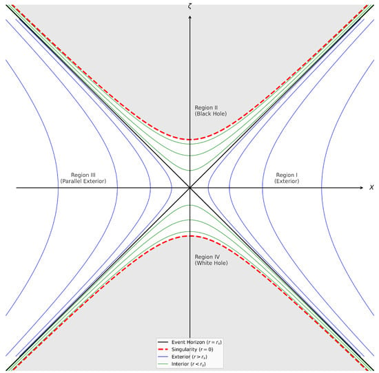
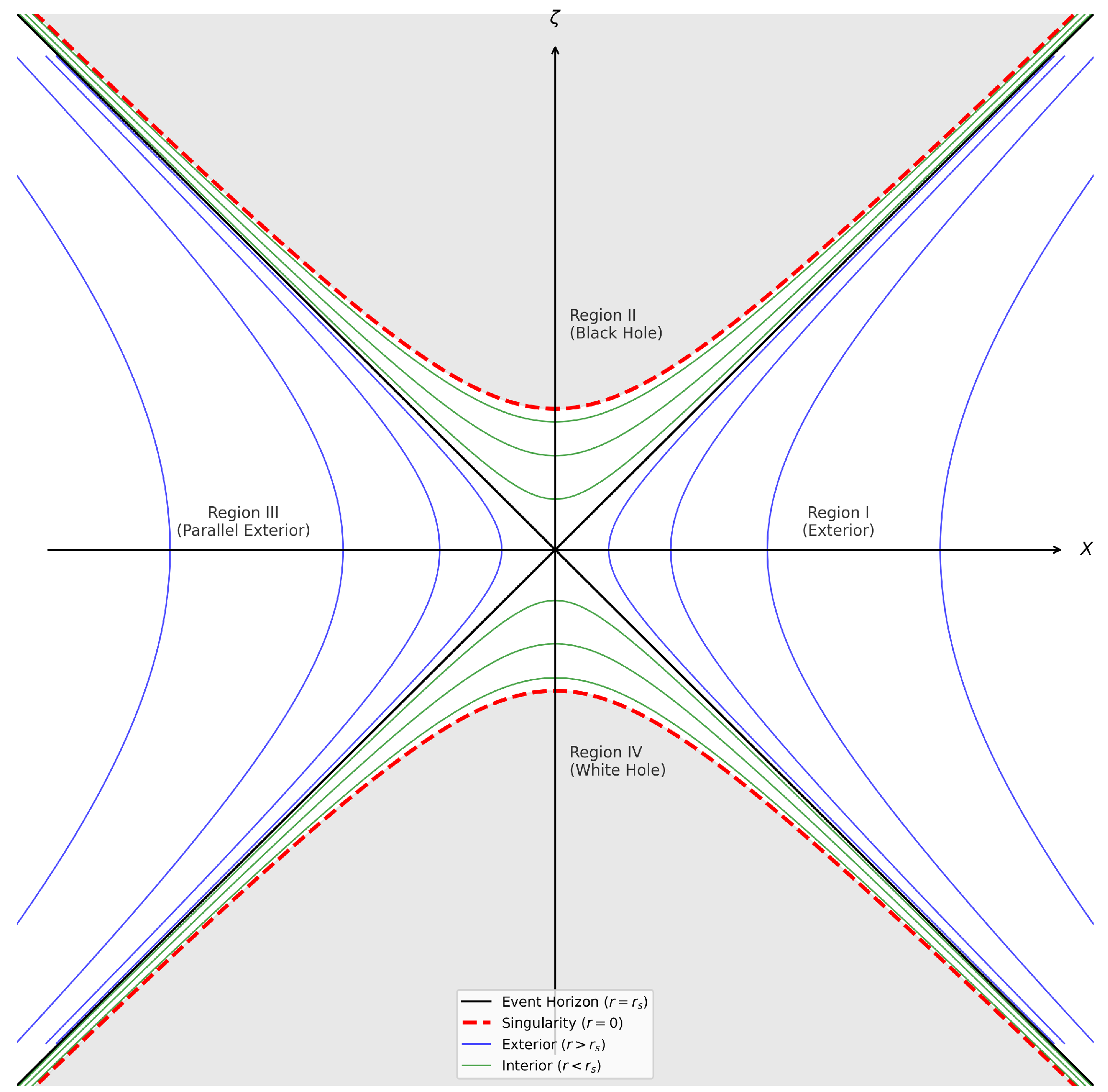
The transformations (19) are associated to the exterior region of the black hole (see Figure 2). Note the striking similarities when deriving the Tortoise and Kruskal coordinates, since both describe conformally flat transformations for the first two terms of Equation (3).

Figure 2. Maximally extended Schwarzschild spacetime from the Kruskal representation.

There are other possible representations with this conformally flat (1+1) feature. In particular, a compact representation of the Schwarzschild spacetime is obtained by the pulsating coordinates, recently defined in Ref. [15]. Instead of hyperbolic trigonometric functions, they are defined in terms of trigonometric functions as

$$\begin{array}{c}\xi =D\sin \left({\displaystyle \frac{t}{\alpha }}\right)\cos \left({\displaystyle \frac{r^{\ast }}{\alpha }}\right),\\ \\ \chi =D\cos \left({\displaystyle \frac{t}{\alpha }}\right)\sin \left({\displaystyle \frac{r^{\ast }}{\alpha }}\right),\end{array}$$

(22)

where D and $\alpha$ are constants with units of distance.

Under these transformations, the metric in Equation (3) becomes equivalent to

$$d{s}^2=\varpi \left(-d{\xi }^2+d{\chi }^2\right)+r^{2}d{\mathrm{\Omega }}^2,$$

(23)

where the (1+1) conformal factor is now

$$\varpi ={\displaystyle \frac{2{\alpha }^2\gamma }{D^2}}{\left[\cos \left({\displaystyle \frac{2t}{\alpha }}\right)+\cos \left({\displaystyle \frac{2r^{\ast }}{\alpha }}\right)\right]}^{-1}.$$

(24)

From the transformations (22), one finds

$${\displaystyle \frac{{\xi }^2}{{\cos }^2\left(\frac{r^{\ast }}{\alpha }\right)}}+{\displaystyle \frac{{\chi }^2}{{\sin }^2\left(\frac{r^{\ast }}{\alpha }\right)}}=D^2.$$

(25)

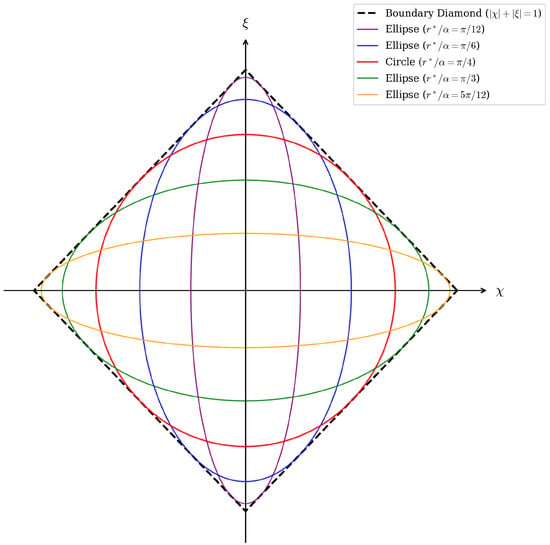
We now have ellipses, instead of hyperbolas. The constants D and $\alpha$ govern the amplitude of the representation in a $(\xi ,\chi )$ diagram, and the modulation of how rapidly the ellipses change as r varies. Similarly, in the Kruskal representation, the amplitude of the hyperbolas determines the placement of the upper hyperbola ${\zeta }^2-X^2=1$ in Figure 2, while the constant $2r_s$ inside the functions in (19) determines the pace at which the hyperbolas evolve as they approach $r=r_s$. In this sense, we set $D=1$ to get the representation in Figure 3.

Figure 3. Compact diamond representation of the Schwarzschild spacetime.

The four corners of the diamond region are located at $(\xi ,\chi )=(\pm 1,\pm 1)$. Equation (25) allows us to trace changes in the geometry, starting from a positive value $r^{\ast }/\alpha$. We choose $\alpha =(2/\pi )({\phi }^{+}-\ln {\phi }^{+})r_s$, where ${\phi }^{+}=(1+\sqrt{5})/2$. This constant is such that when $r^{\ast }/r_s={\phi }^{+}-\ln {\phi }^{+}\approx 1.1368$, we have $r^{\ast }/\alpha =\pi /2$, which yields the horizontal degenerate ellipse (a line segment) at $\xi =0$, with $-1\le \chi \le 1$. This arbitrary initial selection corresponds to the location $r={\phi }^{+}{r}_s\approx 1.618r_s$. While this specific value does not represent a geometric invariant of the Schwarzschild spacetime, it emerges as a mathematically distinguished point in the graphical parametrization of the golden representation discussed below. Decreasing r yields horizontal ellipses that become progressively less elongated. When $r^{\ast }/\alpha =\pi /4$—which in our selection corresponds to the sphere at $r\approx 1.5922r_s$—the geometry is represented in the diagram by a circle. Continuing to lower values of r produces vertical ellipses that become increasingly elongated until reaching the vertical degenerate ellipse bounded by $\xi =\pm 1$ at $r^{\ast }=0$. Decreasing r repeats the inverse process, and this cycle continues infinitely many times as $r\to r_s$.

Let us expand on the meaning of the infinite oscillations. The pulsating transformations (22), defining the diamond representation, rely on the periodic functions $\xi -\chi =D\sin (u/\alpha )$ and $\xi +\chi =D\sin (v/\alpha )$, where $u=t-r^{\ast }$ and $v=t+r^{\ast }$ are null coordinates. Because the sine functions are periodic, this transformation is inherently non-invertible globally; it wraps the $(t,r^{\ast })$ plane over the same coordinate patches infinitely many times. To achieve invertibility, the map must be strictly restricted to a single fundamental coordinate patch, for instance, $-\pi /2<u/\alpha <\pi /2$ and $-\pi /2<v/\alpha <\pi /2$. The Jacobian of the transformation vanishes precisely at the boundary of this mapped region ($\xi \pm \chi =\pm D$). Furthermore, this periodicity dictates an unusual asymptotic behavior at both boundaries of the exterior spacetime. If one holds t fixed, taking either the horizon limit ($r\to r_s\Rightarrow r^{\ast }\to -\infty$) or the spatial infinity limit ($r\to \infty \Rightarrow r^{\ast }\to +\infty$) causes the coordinates u and v to diverge to $\pm \infty$. Consequently, the sine functions oscillate indefinitely in both limits. Therefore, in the diamond representation, neither the event horizon nor spatial infinity converge to a unique boundary curve. Rather, approaching either physical limit causes the map to cycle infinitely through the same concentric ellipses.

We have reviewed some classical representations of the Schwarzschild spacetime, such as the Flamm paraboloid and the tortoise and Kruskal transformations. We also presented the pulsating coordinates, recently proposed as a natural extension of these classical mappings [15]. In turn, the pulsating coordinates have motivated the causal diamond coordinates as an alternative to the customary Rindler representation of Minkowski spacetime [24]. Let us now explore the golden representation.

4. Obtaining the Golden Coordinates

Start with a generic spherically symmetric static form, given by

$$d{\tilde{s}}^2=-e^{2\alpha \left(x\right)}d{t}^2+e^{2\beta \left(x\right)}d{x}^2+e^{2\gamma \left(x\right)}d{\mathrm{\Omega }}^2.$$

(26)

Here, we are defining the dimensionless variable $x=r/r_s$, and we consider that $d{\tilde{s}}^2$ is related with the metric (3) by $d{\tilde{s}}^2=d{s}^2/r_s^2$. The Christoffel symbols are calculated from

$${\mathrm{\Gamma }}_{\mu \nu }^{\alpha }={\displaystyle \frac{1}{2}}{g}^{\alpha \lambda }({\partial }_{\mu }{g}_{\lambda \nu }+{\partial }_{\nu }{g}_{\mu \lambda }-{\partial }_{\lambda }{g}_{\mu \nu }).$$

(27)

The non-trivial ones are

$$\begin{array}{ccc}{\mathrm{\Gamma }}_{01}^0={\displaystyle \frac{d\alpha }{dx}},\hfill & {\mathrm{\Gamma }}_{00}^1=e^{2(\alpha -\beta )}{\displaystyle \frac{d\alpha }{dx}},\hfill & {\mathrm{\Gamma }}_{11}^1={\displaystyle \frac{d\beta }{dx}},\hfill \\ {\mathrm{\Gamma }}_{22}^1=-e^{2(\gamma -\beta )}{\displaystyle \frac{d\gamma }{dx}}\hfill & {\mathrm{\Gamma }}_{33}^1=-{\sin }^2\theta e^{2(\gamma -\beta )}{\displaystyle \frac{d\gamma }{dx}},\hfill & {\mathrm{\Gamma }}_{12}^2={\displaystyle \frac{d\gamma }{dx}},\hfill \\ {\mathrm{\Gamma }}_{33}^2=-\sin \theta \cos \theta ,\hfill & {\mathrm{\Gamma }}_{13}^3={\displaystyle \frac{d\gamma }{dx}},\hfill & {\mathrm{\Gamma }}_{23}^3=\cot \theta ,\hfill \end{array}$$

(28)

as well as those related by ${\mathrm{\Gamma }}_{\alpha \beta }^{\mu }={\mathrm{\Gamma }}_{\beta \alpha }^{\mu }$. Now, we substitute them into

$$R_{\mu \nu }={\partial }_{\alpha }{\mathrm{\Gamma }}_{\mu \nu }^{\alpha }-{\partial }_{\nu }{\mathrm{\Gamma }}_{\mu \alpha }^{\alpha }+{\mathrm{\Gamma }}_{\alpha \lambda }^{\alpha }{\mathrm{\Gamma }}_{\mu \nu }^{\lambda }-{\mathrm{\Gamma }}_{\nu \lambda }^{\alpha }{\mathrm{\Gamma }}_{\mu \alpha }^{\lambda }.$$

(29)

The Ricci tensor components distinct of zero are then

$$\begin{array}{c}{R}_{00}=e^{2(\alpha -\beta )}\left[{\displaystyle \frac{d^2\alpha }{d{x}^2}}+{\displaystyle \frac{d\alpha }{dx}}{\displaystyle \frac{d(\alpha -\beta +2\gamma )}{dx}}\right],\\ R_{11}={\displaystyle \frac{d\alpha }{dx}}{\displaystyle \frac{d(\beta -\alpha )}{dx}}+2{\displaystyle \frac{d\gamma }{dx}}{\displaystyle \frac{d(\beta -\gamma )}{dx}}-{\displaystyle \frac{d^2\left(\alpha +2\gamma \right)}{d{x}^2}}.\\ R_{22}=1+e^{2(\gamma -\beta )}\left[{\displaystyle \frac{d(\beta -\alpha -2\gamma )}{dx}}{\displaystyle \frac{d\gamma }{dx}}-{\displaystyle \frac{d^2\gamma }{d{x}^2}}\right],\\ R_{33}={\sin }^2\theta R_{22}.\end{array}$$

(30)

Finally, the scalar curvature $R=g^{\mu \nu }{R}_{\mu \nu }$ results in

$$R=2e^{-2\beta }\left[{\displaystyle \frac{d(\beta -\alpha )}{dx}}{\displaystyle \frac{d\left(\alpha +2\gamma \right)}{dx}}-{\displaystyle \frac{d^2\left(\alpha +2\gamma \right)}{d{x}^2}}-3{\left({\displaystyle \frac{d\gamma }{dx}}\right)}^2\right]+2e^{-2\gamma }.$$

(31)

The Einstein–Hilbert action is $16\pi S=\int \sqrt{-g}R{d}^{4}x$. Since $\sqrt{-g}=e^{\alpha +\beta +2\gamma }\sin \theta$, omitting a constant factor, we are interested in the integral with respect to r of

$${\displaystyle \frac{e^{\alpha -\beta +2\gamma }}{2}}\left[{\displaystyle \frac{d(\beta -\alpha )}{dx}}{\displaystyle \frac{d\left(\alpha +2\gamma \right)}{dx}}-{\displaystyle \frac{d^2\left(\alpha +2\gamma \right)}{d{x}^2}}-3{\left({\displaystyle \frac{d\gamma }{dx}}\right)}^2\right]+{\displaystyle \frac{e^{\alpha +\beta }}{2}}.$$

(32)

This functional allows us to use the Euler–Lagrange equations. Up to a total derivative, it is equivalent to the (radial) Lagrangian as follows:

$$L_r={\displaystyle \frac{e^{\alpha -\beta +2\gamma }}{2}}\left[2{\displaystyle \frac{d\alpha }{dx}}{\displaystyle \frac{d\gamma }{dx}}+{\left({\displaystyle \frac{d\gamma }{dx}}\right)}^2\right]+{\displaystyle \frac{e^{\alpha +\beta }}{2}}.$$

(33)

We define the “coordinates” $q^1=\gamma$ and $q^2=\alpha$. Then, we rewrite $L_r$ as

$$L={\displaystyle \frac{{\lambda }^{-1}}{2}}\left[{\left({\dot{q}}^1\right)}^2+2{\dot{q}}^1{\dot{q}}^2\right]+{\displaystyle \frac{\lambda }{2}}{M}^2,$$

(34)

where we have further defined ${\lambda }^{-1}=e^{\alpha -\beta +2\gamma }$ and $M^2={\lambda }^{-1}{e}^{\alpha +\beta }=e^{2\alpha +2\gamma }$. Additionally, for simplicity, we use dot notation for total derivatives with respect to x, as in ${\dot{q}}^1=d{q}^1/dx$. This suggestive form allows us to treat this Lagrangian as describing a relativistic point particle in two dimensions in the form $\left({\lambda }^{-1}{Q}_{ab}{\dot{q}}^a{\dot{q}}^b+\lambda M^2\right)/2$, where $a,b$ run over $\{1,2\}$. We call $Q_{ab}$ the Fibonacci Q-metric, with components

$$Q_{ab}=\left(\begin{array}{cc}1& 1\\ 1& 0\end{array}\right).$$

(35)

We use $q^1$, $q^2$ and $\lambda$ as independent variables. Variations with respect to $q^1$ and $q^2$ lead to

$${\displaystyle \frac{d}{dx}}\left[{\lambda }^{-1}\left({\dot{q}}^1+{\dot{q}}^2\right)\right]=\lambda M^2,$$

(36)

and

$${\displaystyle \frac{d}{dx}}\left({\lambda }^{-1}{\dot{q}}^1\right)=\lambda M^2,$$

(37)

respectively, where we use $\partial M^2/\partial q^a=2M^2$. The variation with respect to $\lambda$ yields

$${\lambda }^{-2}\left[{\left({\dot{q}}^1\right)}^2+2{\dot{q}}^1{\dot{q}}^2\right]=M^2.$$

(38)

These equations are consistent with those obtained directly from the original Einstein–Hilbert action [21]. In fact, Equations (36) and (37) together imply

$${\displaystyle \frac{d\left({\lambda }^{-1}{\dot{q}}^2\right)}{dx}}=0.$$

(39)

From the definitions of the coordinates and ${\lambda }^{-1}=e^{\alpha -\beta +2\gamma }$, one can verify that Equation (39) is equivalent to the field equation $R_{00}=0$, which can be read from (30).

Also, by using Equations (38) and (39) in Equation (36), one obtains

$${\displaystyle \frac{d}{dx}}\left[\ln \left({\lambda }^{-1}{\dot{q}}^1\right)-q^1-2q^2\right]=0.$$

(40)

This is equivalent to ${\lambda }^{-1}{\dot{q}}^1=2K{e}^{q^1+2q^2}$, where K is a constant. Returning to the original variables, this is the same as $d\left(e^{\gamma }\right)/dx=K{e}^{\alpha +\beta }$. We can use this intermediate result in ${\lambda }^{-1}{\dot{q}}^2=const.$ [cf. (39)] to show that this implies

$$e^{2\alpha }=e^{2q^2}=c_1-c_2{e}^{-q^1},$$

(41)

where $c_1$ and $c_2$ are constants. Again, if one sets $e^{q^1}=e^{\gamma }=x=r/r_s$ in the metric (26), one recovers the result $\beta =-\alpha$, with $K=1$. By asymptotic flatness, Equation (41) is the familiar Schwarzschild factor $1-r_s/r=-g_{00}$. We have completed the correspondence with classical results. Starting from the static, spherically symmetric ansatz in Equation (26), the reduced variational field equations recover the standard Schwarzschild solution within this restricted class. We note that because our starting ansatz assumes staticity, this calculation does not constitute a proof of Birkhoff’s theorem (which proves that spherical vacuum symmetry uniquely implies staticity). As shown by Deser and Franklin [42], obtaining Birkhoff’s theorem from a reduced action requires retaining explicit time dependence in the metric functions.

The eigenvalues of the metric (35) are ${\phi }^{-}=(1-\sqrt{5})/2$ and ${\phi }^{+}=(1+\sqrt{5})/2$: the negative and positive golden ratios (see Appendix A). It is important to note that these specific numerical eigenvalues are not geometric invariants of the spacetime; rather, metric components transform by congruence, and these eigenvalues depend on our specific choice of parametrization for $q_1$ and $q_2$. However, in this chosen normalization, the kinetic metric elegantly takes this Fibonacci form, preserving the invariant Lorentzian signature.

By calculating the eigenvectors of $Q_{ab}$, one can see that the coordinate transformations

$$\begin{array}{c}{w}^1={\displaystyle \frac{1}{5^{1/4}}}\left(\sqrt{-{\phi }^{-}}{q}^1-\sqrt{{\phi }^{+}}{q}^2\right),\\ \\ w^2={\displaystyle \frac{1}{5^{1/4}}}\left(\sqrt{{\phi }^{+}}{q}^1+\sqrt{-{\phi }^{-}}{q}^2\right),\end{array}$$

(42)

imply the equality $Q_{ab}d{q}^{a}d{q}^b=G_{ab}d{w}^{a}d{w}^b$, where we define

$$G_{ab}=\left(\begin{array}{cc}{\phi }^{-}& 0\\ 0& {\phi }^{+}\end{array}\right).$$

(43)

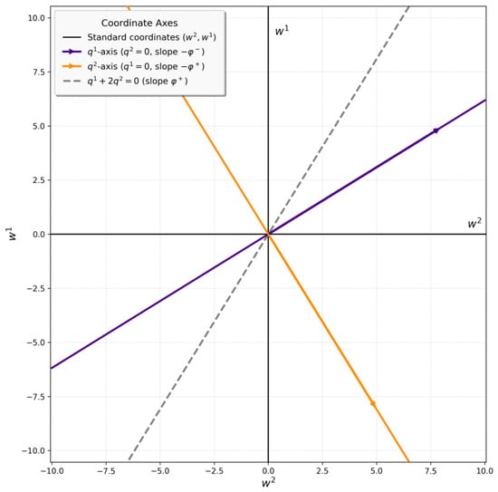
Rescaling coordinates in the form $W^1=\sqrt{-{\phi }^{-}}{w}^1$, $W^2=\sqrt{{\phi }^{+}}{w}^2$, we obtain the usual (1+1)-Minkowski form ${\eta }_{ab}d{W}^{a}d{W}^b$, where ${\eta }_{ab}=diag(-1,1)$ (see Figure 4).

Figure 4. The coordinate transformation from $w^a$ to $q^a$.

The transformation (42) preserves the scale. Here, ‘preserving the scale’ refers to the invariance of the Euclidean norm of the parameter vector in this auxiliary space.

The inversion of Equation (42) is

$$\begin{array}{c}{q}^1={\displaystyle \frac{1}{5^{1/4}}}\left(\sqrt{-{\phi }^{-}}{w}^1+\sqrt{{\phi }^{+}}{w}^2\right),\\ q^2={\displaystyle \frac{1}{5^{1/4}}}\left(-\sqrt{{\phi }^{+}}{w}^1+\sqrt{-{\phi }^{-}}{w}^2\right).\end{array}$$

(44)

Equations (42) and (44) represent $SO\left(2\right)$ rotations acting on the auxiliary Euclidean space of the components, rather than Lorentz transformations of the physical spacetime.

From Equation (44), the $q^1$ and $q^2$ axes have slopes $∆w^1/∆w^2$ equal to $-{\phi }^{-}$ and $-{\phi }^{+}$, respectively. Since ${\phi }^{+}{\phi }^{-}=-1$, they are orthogonal in the diagram. The rotation is by an angle $\arctan {\phi }^{+}\approx 58.28°$. From (34), (35) and (43), one has $G_{ab}d{w}^{a}d{w}^b=Q_{ab}d{q}^{a}d{q}^b=d{q}^1(d{q}^1+2d{q}^2)$. Setting it to zero yields the coordinates $q^1$ and $q^1+2q^2$. Both define directions whose gradients are null with respect to the inverse configuration-space metric. Equivalently, $G_{ab}d{w}^{a}d{w}^b=-{\left(\sqrt{-{\phi }^{-}}d{w}^1\right)}^2+{\left(\sqrt{{\phi }^{+}}d{w}^2\right)}^2$ admits a direct factorization (see Appendix A). In this diagram, lines $q^1=const.$ (as the $q^2$ orange axis) have a slope of $-{\phi }^{+}$ with respect to the horizontal, while $q^1+2q^2=const.$ represents lines with slope ${\phi }^{+}$ as the gray line.

For completeness, now we work directly in the golden representation.

5. Kinematics in the Golden Representation

So far, we have shown the dimensional reduction from the (1+3) dynamical Einstein–Hilbert action to a radial (1+1) equivalent Lagrangian. We can now show explicitly how the trajectories in this auxiliary configuration space correspond to the original Schwarzschild geometry, provided we impose staticity, fix the radial gauge, and select the correct integration constants. As we have shown, the Lagrangian (34) is the same as

$$L_r={\displaystyle \frac{{\lambda }^{-1}}{2}}{Q}_{ab}{\dot{q}}^a{\dot{q}}^b+{\displaystyle \frac{\lambda }{2}}{M}^2,$$

(45)

where $Q_{ab}$ is the Q-Fibonacci metric in Equation (35), while ${\lambda }^{-1}=e^{-\beta }{e}^{2q^1+q^2}$ and $M=e^{q^1+q^2}$. Recall also the equality $Q_{ab}{\dot{q}}^a{\dot{q}}^b=G_{ab}{\dot{w}}^a{\dot{w}}^b$, where we have the two equivalent forms (35) and (43). While $(w^1,w^2)$ are explicit orthogonal coordinates in this (1+1) version, $(q^1,q^2)$ are the ones with a direct translation in terms of both the Schwarzschild and the tortoise coordinates.

Equation (38) is equivalent to $Q_{ab}{\dot{q}}^a{\dot{q}}^b={\lambda }^2{M}^2$, which is also obtained by varying the action into which (45) is inserted, with respect to $\lambda$. In this (1+1)-dimensional system, the gauge $\lambda =M^{-1}$ would be the equivalent to taking the normalization $Q_{ab}{\dot{q}}^a{\dot{q}}^b=1$ for the tangent vector $d{q}^a/dx$. However, the association with Schwarzschild geometry requires another norm, as we shall see. This norm is spacelike, in agreement with all the previous comments about our fictitious particle system. With all this in mind, we substitute $\lambda =M^{-1}\sqrt{Q_{ab}{\dot{q}}^a{\dot{q}}^b}$ in (45), leading to

$$L_r=M\sqrt{Q_{ab}{\dot{q}}^a{\dot{q}}^b}.$$

(46)

This is very similar to the relativistic point particle, although M is not constant. As variations in (46) lead to the geodesics of this system, we define $\tilde{\mathrm{\Phi }}$ as an auxiliary configuration-space metric: the golden metric. It incorporates the conformal factor $M^2$ as

$$d{\sigma }^2={\mathrm{\Phi }}_{ab}d{q}^{a}d{q}^b=M^2{Q}_{ab}d{q}^{a}d{q}^b.$$

(47)

This is a metric on the two-dimensional radial minisuperspace, not a spacetime metric obtained from Schwarzschild by a coordinate transformation. In terms of the coordinates defined below (43), this is conformal Minkowski, as $M^2{\eta }_{ab}d{W}^{a}d{W}^b$. Here, the two-dimensional version of (27) is equivalent to a differential operator acting on $\ln M$ [25], as follows:

$${\mathrm{\Gamma }}_{ab}^c=({\delta }_b^c{\partial }_a+{\delta }_a^c{\partial }_b-Q^{cd}{Q}_{ab}{\partial }_d)\ln M.$$

(48)

We thus use ${\partial }_a=\partial /\partial q^a$, and $Q^{cd}$ is such that $Q^{cd}{Q}_{bd}={\delta }_b^c$. Given $M=e^{q^1+q^2}$, one has that ${\partial }_a\ln M=1$. Thus, Equation (48) is the same as ${\mathrm{\Gamma }}_{ab}^c={\delta }_a^c+{\delta }_b^c-Q^{cd}{Q}_{ab}\left({\delta }_d^1+{\delta }_d^2\right)$.

The Q-Fibonacci metric (35) is $Q_{ab}={\delta }_a^1{\delta }_b^1+2{\delta }_{(a}^1{\delta }_{b)}^2$, where parentheses indicate symmetrization as in $A_{\left(ab\right)}=\left(A_{ab}+A_{ba}\right)/2$. The inverse Q-metric can be expressed as $Q^{cd}=2{\delta }_1^{(c}{\delta }_2^{d)}-{\delta }_2^c{\delta }_2^d$, implying $Q^{cd}\left({\delta }_d^1+{\delta }_d^2\right)={\delta }_1^c$. Then, (48) is

$${\mathrm{\Gamma }}_{ab}^c={\delta }_a^c+{\delta }_b^c-{\delta }_1^c\left(1-{\delta }_a^2{\delta }_b^2\right).$$

(49)

The non-zero Christoffel symbols are ${\mathrm{\Gamma }}_{11}^1={\mathrm{\Gamma }}_{12}^2={\mathrm{\Gamma }}_{21}^2=1$ and ${\mathrm{\Gamma }}_{22}^2=2$. The geodesic equation ${\ddot{q}}^c+{\mathrm{\Gamma }}_{ab}^c{\dot{q}}^a{\dot{q}}^b=0$ yields

$${\ddot{q}}^1+{\left({\dot{q}}^1\right)}^2=0$$

(50)

and

$${\ddot{q}}^2+2\left({\dot{q}}^1+{\dot{q}}^2\right){\dot{q}}^2=0.$$

(51)

Equation (50) can be solved by defining $\zeta ={\dot{q}}^1$, which makes ${\ddot{q}}^1=d\zeta /dx={\dot{q}}^1(d\zeta /d{q}^1)$. One obtains the linear equation $d\zeta /d{q}^1+\zeta =0$. Since the solution is ${\dot{q}}^1=\zeta \propto e^{-q^1}$, this in turn implies that the solution to (50) is

$$e^{q^1}=Ax+B,$$

(52)

where A and B are constants. Let us set $B=0$ and $A=1$, and recall that $x=r/r_s$ in Equation (26). With these selections, $e^{q^1}=r/r_s$ and ${\dot{q}}^1=r_s/r$. Equation (51) can also undergo an order reduction by defining $h={\dot{q}}^2$, yielding the equivalent form

$$\dot{h}+{\displaystyle \frac{2}{x}}h+2h^2=0.$$

(53)

With a further definition $h=u^{-1}$, $\dot{h}=-u^{-2}\dot{u}$, Equation (53) is equivalent to $\dot{u}-2x^{-1}u=2$. This is the same as $d\left(r^{-2}u\right)/dx=2r^{-2}$, which integrates to $u=-2x+D{x}^2$, with D another integration constant. Since ${\dot{q}}^2=u^{-1}$,

$${\displaystyle \frac{d{q}^2}{dx}}={\displaystyle \frac{1}{x(Dx-2)}}={\displaystyle \frac{1}{2}}\left({\displaystyle \frac{D}{Dx-2}}-{\displaystyle \frac{1}{x}}\right),$$

(54)

with solution $q^2=\ln \sqrt{D-{\displaystyle \frac{2}{x}}}+const.$ Setting $D=2$ and $const.=2^{-1}\ln \left(2^{-1}\right)$, one obtains

$$q^2=\ln \sqrt{1-{\displaystyle \frac{r_s}{r}}}.$$

(55)

That is, we have recovered $e^{q^1}=r/r_s$ and also $e^{q^2}=\sqrt{1-r_s/r}$, the redshift factor. That is, the selection of constants in the solutions to the kinematic equations of this (1+1) geometry yields the common Schwarzschild solution, when associating it with the (1+3) version in an appropriate way. The association is completed if one recalls [below (45)] that $\lambda =e^{\beta }{e}^{-(2q^1+q^2)}$ and $M=e^{q^1+q^2}$. It follows that the result $\alpha =q^2=-\beta$ is consistent with choosing a gauge where $\lambda =e^{\beta }{e}^{-q^1}/M=e^{-2(q^1+q^2)}=1/M^2$.

The association of the kinematics of the Lagrangian (46) with the dynamic equations for the metric (26) can be summarized as follows:

• Golden (1+1) kinematics⟺(1+3)-Schwarzschild dynamics.

Note how the constants have been selected: In (52), setting $A=1$ and $B=0$ allows us to have the proper association between (26) and (3). Also, selecting $D=2$ and the last constant mentioned above Equation (55) allows a factoring that also connects the coordinate $q^2$ with the Schwarzschild solution. Then, $q^1=\ln (r/rs)$ and $q^2=\ln \sqrt{1-r_s/r}$ yield the usual $e^{2\gamma }$ and $e^{2\alpha }$, leading from Equation (2) to Equation (3) [25].

We choose, from the family of solutions, the following:

$$e^{2q^2}=1-e^{-q^1}.$$

(56)

This is Equation (41), with $c_1=c_2=1$. The event horizon $r=r_s$ is pushed to $(q^1,q^2)\to (0,-\infty )$, similar to the tortoise coordinate behavior.

Although the golden representation lies in the kinematics induced by the golden metric (47) and its connection with the four-dimensional Schwarzschild solution, a legitimate question is the following: what are the intrinsic geometric properties of this fictitious (1+1) spacetime? The short answer is that it is a flat spacetime. As we saw below Equation (49), we have four non-trivial Christoffel symbols for the metric components in (47), ${\mathrm{\Phi }}_{ab}=e^{2(q^1+q^2)}{Q}_{ab}$, given by ${\mathrm{\Gamma }}_{11}^1={\mathrm{\Gamma }}_{12}^2=1$, ${\mathrm{\Gamma }}_{22}^2=2$. Since they are constant, the Riemann tensor for this two-dimensional induced spacetime simplifies to ${\tilde{R}}_{bcd}^a={\mathrm{\Gamma }}_{ce}^a{\mathrm{\Gamma }}_{bd}^e-{\mathrm{\Gamma }}_{de}^a{\mathrm{\Gamma }}_{bc}^e$. Evaluating the Riemann tensor directly with these constant Christoffel symbols yields zero, confirming that this radial minisuperspace is strictly flat.

The explicit transformation to the Minkowski form can be seen by writing the metric (47) in terms of the null-type coordinates discussed in the last part of Section 4, as $d{\sigma }^2=e^{2(q^1+q^2)}d{q}^1(d{q}^1+2d{q}^2)$. Since it can be factored in $dU=e^{q^1}d{q}^1$ and $dV:=-e^{(q^1+2q^2)}(d{q}^1+2d{q}^2)$, we can make $d{\sigma }^2=-dUdV$. Rotating coordinates in the form $dV=dT-dX$ and $dU=dT+dX$ yields the Minkowski form $d{\sigma }^2=-d{T}^2+d{X}^2$. The inversion of coordinates is $T=e^{q^1}(1-e^{2q^2})/2$ and $X=e^{q^1}(1+e^{2q^2})/2$. By using (56) and $e^{q^1}=r/r_s$, this Minkowski form, under translation, is the same as $T=1/2$ and $X=r/r_s-1/2$, which in fact can be rescaled and translated. The special geodesic solution (56), which represents the Schwarzschild spacetime, corresponds to a simple “simultaneity surface” in this Minkowski (1+1) representation, where the space dimension grows linearly with r.

We end this section by remarking that there is a third equivalent Lagrangian to (45) and (46) [21]. Consider the Legendre transform of (45):

$$H_A={\dot{q}}^a{p}_a-L_r,$$

(57)

where $p_a=\partial L_r/\partial {\dot{q}}^a$. From (45), we obtain $p_1={\lambda }^{-1}\left({\dot{q}}^1+{\dot{q}}^2\right)$ and $p_2={\lambda }^{-1}{\dot{q}}^1$. We use their inversions to eliminate the ${\dot{q}}^a$-dependence in (57):

$$H_A={\displaystyle \frac{\lambda }{2}}\left[\left(2p_1-p_2\right)p_2-M^2\right].$$

(58)

In terms of the $p^a$, the Lagrangian (45) satisfies $2L_r=\lambda \left(2p_1-p_2\right)p_2+\lambda M^2$. Then, (58) is equivalent to $L_r=H_A+\lambda M^2$. Recalling [above Equation (49)] the inverse of (35), $Q^{cd}=2{\delta }_1^{(c}{\delta }_2^{d)}-{\delta }_2^c{\delta }_2^d$, we can use (57) again to simplify $L_r$ to

$$L_r={\dot{q}}^a{p}_a-{\displaystyle \frac{\lambda }{2}}\left(p_a{p}_b{Q}^{ab}-M^2\right).$$

(59)

This form for $L_r$ now depends on the momenta $p^a$. Nevertheless, it allows for variations with respect to $\lambda$, which yields the constraint $p_a{p}_b{Q}^{ab}=M^2$. By making the translations as before, in particular the identification $\lambda \left(2p_1-p_2\right)p_2={\lambda }^{-1}{Q}_{ab}{\dot{q}}^a{\dot{q}}^b$, this Hamiltonian constraint is the same as $Q_{ab}{\dot{q}}^a{\dot{q}}^b={\lambda }^2{M}^2$, used for the development of this section.

Now, let us turn our attention to some visualizations of the Schwarzschild radial geometry in the $q^a$ representation.

6. Visual Golden Representations

The golden representation of the Schwarzschild geometry in (3) can be understood in a similar way to the Flamm paraboloid in Figure 1, defined by the functions $(\rho ,z)=\left(r,\sqrt{4r_s\left(r-r_s\right)}\right)$. In our present case, the golden coordinates for the Schwarzschild spacetime are $\left(q^1,q^2\right)=\left(\ln \left(r/r_s\right),\ln \sqrt{1-r_s/r}\right)$. In the (0+2) Flamm representation of Equation (9), evaluating the interval from $r=r_s$ to $r\to \infty$ corresponds to $(\rho ,z)$ going from $(r_s,0)$ to $(\infty ,\infty )$. In the (1+1) golden representation, the corresponding limits are from $(q^1,q^2)\to (0,-\infty )$ to $(q^1,q^2)\to (\infty ,0)$.

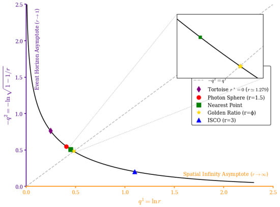
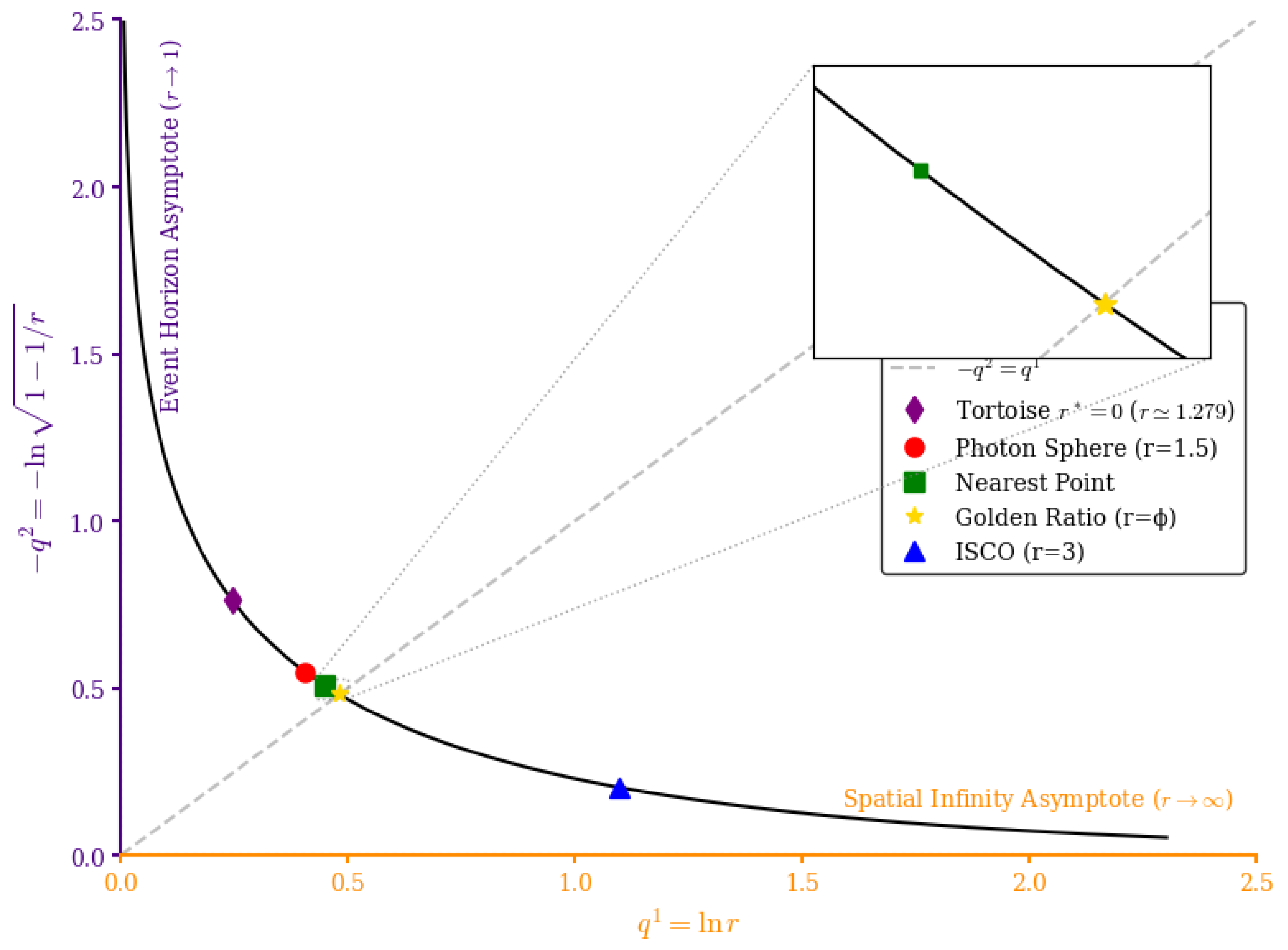
Figure 5 shows the golden representation of spatial sections of the Schwarzschild geometry. As compared to Figure 4, the axes are rotated, followed by an inversion. Some points are explicitly marked, such as the location where $r^{\ast }=0$ ($r\approx 1.2786r_s$), the photon sphere at $r=3r_s/2$, the golden radius ($r={\phi }^{+}\approx 1.618r_s$), and the ISCO (Innermost Stable Circular Orbit) at $r=3r_s$. Recall that in the diamond representation (Figure 3), we chose to change ellipses from $r={\phi }^{+}{r}_s$ to the value where $r^{\ast }=0$. In Figure 5, this would represent a change in the curve between the points marked in yellow and purple.

Figure 5. Trajectory of the Schwarzschild geometry in the auxiliary minisuperspace $(q^1,q^2)$. The coordinate projections directly map key physical observables: $q^1=\ln (r/r_s)$ encodes the areal radius, $q^2=\ln \sqrt{1-r_s/r}$ encodes the local redshift, and parallel shifts along $q^1+2q^2=(r^{\ast }-r)/r_s$ isolate the radial travel-time excess discussed in Section 7.

As we have seen, $r={\phi }^{+}{r}_s$ is the point where $q^1=-q^2=\ln {\phi }^{+}$, which corresponds to the intersection of the curve with the bisector line in this quadrant. However, this is not the closest approach to the point $(0,0)$ in Figure 5. While the distance to the curve (indicating $r={\phi }^{+}$) is $\sqrt{2}\ln {\phi }^{+}\approx 0.68054$, the shortest distance (minimizing and numerically solving) is $d\approx 0.67830$. By Equation (42), this point has w-coordinates $(w^1,w^2)={\displaystyle \frac{1}{5^{1/4}}}{\left({\phi }^{+}\right)}^{-3/2}\ln {\phi }^{+}\left[{\left({\phi }^{+}\right)}^3,1\right]$. In Figure 4, the line joining $(0,0)$ to the point representing $r={\phi }^{+}$ has slope ${\left({\phi }^{+}\right)}^3$. This line forms an angle of $\pi /2-(1/2)\arctan (1/2)$ with the horizontal, approximately $76.72°$. There, the family of possible solutions to (41) lies in the region where $q^1>0$, $q^2<0$. There, we can set $c_1=1$ by the asymptotic flatness of the Schwarzschild solution, while the constant $c_2$ modulates r with respect to some radius. By means of (42), the translation to the w-representation is as follows: taking r, from $r_s$ to ∞ corresponds to changing from $(w^1,w^2)\to (\infty ,-\infty )$ to $(w^1,w^2)\to (\infty ,\infty )$. For $r\gg r_s$, they behave as $w^1\simeq 5^{-1/4}\sqrt{-{\phi }^{-}}\ln (r/r_s)$ and $w^2\simeq 5^{-1/4}\sqrt{{\phi }^{+}}\ln (r/r_s)$, and we have the asymptotic behavior $w^1=-{\phi }^{-}{w}^2$. This corresponds to the line $q^1$ in Figure 4. On the other hand, the near-horizon approximation $r\approx r_s$ has the asymptotic behavior $w^1\simeq -{\phi }^{+}{w}^2$, with $w^1\simeq -5^{-1/4}\sqrt{{\phi }^{+}}{q}^2$ and $w^2\simeq 5^{-1/4}\sqrt{-{\phi }^{-}}{q}^2$.

We now use the $w^a$ coordinates to get an alternative representation. Let us first rewrite the transformations (42) as

$$\begin{array}{c}{w}^1=\cos \alpha q^1-\sin \alpha q^2,\\ \\ w^2=\sin \alpha q^1+\cos \alpha q^2,\end{array}$$

(60)

where $\cos \alpha =5^{-1/4}\sqrt{-{\phi }^{-}}$ and $\sin \alpha =5^{-1/4}\sqrt{{\phi }^{+}}$, and the rotation angle is $\arctan {\phi }^{+}$. Recall also that with $W^1=\sqrt{-{\phi }^{-}}{w}^1$ and $W^2=\sqrt{{\phi }^{+}}{w}^2$, one has that $G_{ab}d{w}^{a}d{w}^b={\eta }_{ab}d{W}^{1}d{W}^2$, where $G_{ab}=diag({\phi }^{-},{\phi }^{+})$ and ${\eta }_{ab}=diag(-1,1)$. This motivates performing a Wick rotation for the timelike coordinate $W^1$ as $W^1\to iT$ [43]. This transformation would allow us to consider a complex representation $W^2+i{W}^1$, but in fact, in the complex plane, this would be equivalent to Figure 5. Recalling that (57) preserves the scale between the systems $w^a$ and $q^a$, this instead motivates the introduction of the complex quantity $\sqrt{{\phi }^{+}}{q}^2+i\sqrt{-{\phi }^{-}}{q}^1$. Factoring out $\sqrt{{\phi }^{+}}$, we simply exponentiate $q^2-i{\phi }^{-}{q}^1$, obtaining

$$Z=e^{q^2}{e}^{-i{\phi }^{-}{q}^1}.$$

(61)

A real representation arises by considering that Equation (61) is $Z=\left|Z\right|e^{i\theta }$, where $\theta =-{\phi }^{-}{q}^1$. Given that $q^1=\ln (r/r_s)$, the inversion $r=r_s{e}^{{\phi }^{+}\theta }$ describes a real logarithmic spiral [44].

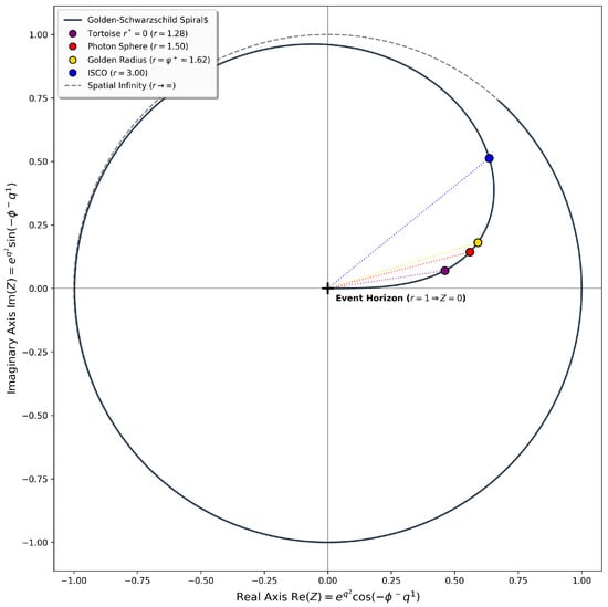
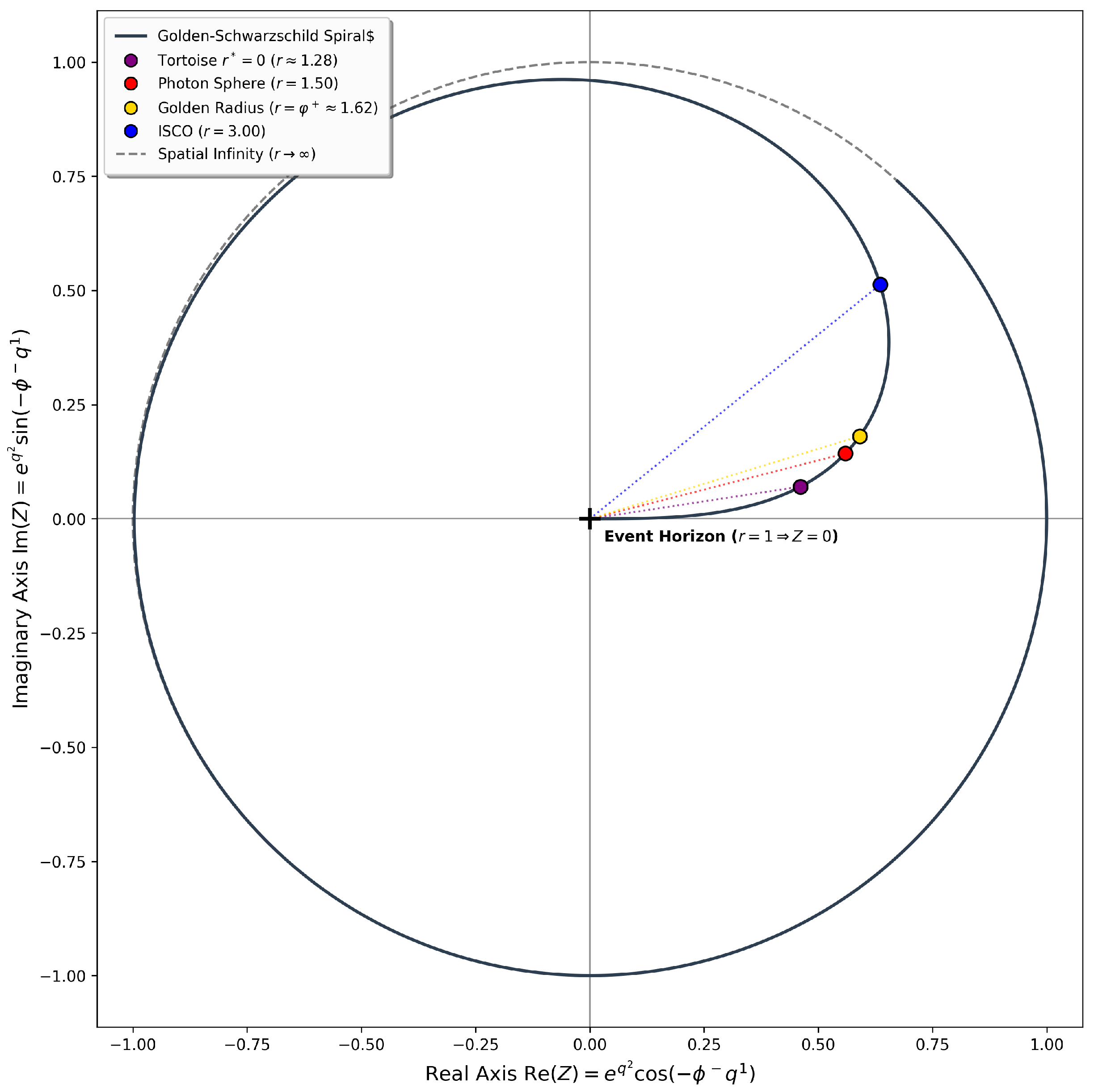
The complex mapping in Equation (61) provides a compact representation of the radial Schwarzschild geometry within the auxiliary framework (see Figure 6). It is important to emphasize that this diagram is a complex transformation of the minisuperspace variables rather than an isometric spatial slice. However, its polar coordinates directly map key physical observables of the spacetime, as follows:

Figure 6. The complex golden-Schwarzschild spiral representation $Z=e^{q^2}{e}^{-i{\phi }^{-}{q}^1}$. The map encodes physical observables into polar coordinates: the radial distance from the origin $\left|Z\right|=e^{q^2}=\sqrt{1-r_s/r}$ measures the gravitational redshift factor, while $\theta =-{\phi }^{-}{q}^1$ parameterizes the radius $r/r_s=e^{{\phi }^{+}\theta }$.

• Gravitational Redshift: The magnitude $\left|Z\right|=e^{q^2}=\sqrt{1-r_s/r}$ measures the local redshift factor directly as the radial distance from the origin (horizon at $Z=0$) to a given point.
• Areal Radius: The angular phase $\theta =-{\phi }^{-}{q}^1$ parameterizes the areal radius $r=r_s{e}^{{\phi }^{+}\theta }$, winding asymptotically toward spatial infinity at $\left|Z\right|=1$.

The previous representative points in Figure 5 are also shown in the golden-Schwarzschild spiral of Figure 6. Consider the point representing $r={\phi }^{+}{r}_s$: its distance to the origin is $\left|Z\right|=\sqrt{1-1/{\phi }^{+}}=-{\phi }^{-}$, which also fulfills $1-{\left|Z\right|}^2=-{\phi }^{-}$. That is, this point has a distance $-{\phi }^{-}\approx 0.618$ from the origin.

The inverse areal radius $r_s/r$, corresponding to the complement of the squared norm $1-{\left|Z\right|}^2$, can also be expressed as a logarithmic spiral, $1-{\left|Z\right|}^2=r_s/r=e^{-{\phi }^{+}\theta }$, where we used (56) in ${\left|Z\right|}^2=e^{2q^2}$.

This diagram allows us to easily spot points where r is of order unity. The first crossing of the vertical axis occurs when $q^1={\phi }^{+}\pi /2$, where $r/r_s=\exp ({\phi }^{+}\pi /2)\approx 12.7$. On the left, the first crossing with the horizontal axis is when $r/r_s=\exp \left({\phi }^{+}\pi \right)\approx 161.3$, while the second crossing with the vertical axis is below, for $r/r_s=\exp (3{\phi }^{+}\pi /2)\approx 2048$.

7. Final Comments: Linking Representations

In this article, we have discussed several representations of the Schwarzschild spacetime: the near-horizon approximation and the Flamm paraboloid, as well as the tortoise, Kruskal, diamond, and golden representations. While the former two are classical representations and the diamond representation is a recent development, the golden representation, building on previous works about the relying radial two-dimensional minisuperspace, is newly introduced in this article.

We have delved into the relationships between these representations. For instance, the Flamm parabola allows us to read the integration of (4), the radial proper distance for the Schwarzschild metric, through the Euclidean distance traveled on the parabola (9). From the Flamm parabola, one can also measure the z distance for $r\cong r_s$ to obtain $\varrho$, the radial Rindler (near-horizon) approximation (7).

We also highlighted a derivation of the tortoise and Kruskal coordinates by considering conformal (1+1) radial sections in the Schwarzschild geometry. The tortoise coordinate (15) appears when considering the Cartesian form, while the Kruskal coordinates appear naturally by executing the analogous developments for a conformal flat Rindler transformation. We then presented the diamond representation, the other main general possibility for these types of transformations [15].

In Section 4, Section 5 and Section 6, we introduced the golden representation, arising from transformations of the Einstein–Hilbert action. The radial Lagrangian resulted in a description similar to the kinematical Lagrangian of a relativistic particle [20,21]. We clarified the significance of this dimensional reduction, discussed issues regarding the correct translation to Schwarzschild coordinates, and proposed some useful visualizations.

Let us make three final remarks about the representations we have explored. The first point is that the golden radius $r={\phi }^{+}{r}_s$ corresponds to the following (see Appendix A):

• The location on the Flamm parabola $(\varrho ,z)=({\phi }^{+},2\sqrt{-{\phi }^{-}})r_s$.
• One of infinitely many radii that yield a horizontal degenerate ellipse in the diamond representation (Figure 3), given the $\alpha$ chosen.
• A tortoise coordinate $r^{\ast }/r_s={\phi }^{+}-\ln {\phi }^{+}$.
• The point $q^1=-q^2=\ln {\phi }^{+}$ of the golden representation (Figure 5).
• A location $Z=-{\phi }^{-}{e}^{-i{\phi }^{-}\ln {\phi }^{+}}$ in the complex representation (Figure 6).

It is important to acknowledge that the eigenvalues ${\phi }^{\pm }$ of the minisuperspace metric $Q_{ab}$ depend on our chosen normalization of the reduced variables, and are not coordinate-independent spacetime invariants. But, our parametrization naturally selects the distinguished radius $r={\phi }^{+}{r}_s$ (where $q_1=-q_2$, or $r\sqrt{-g_{00}}=r_s$). While this radius does not represent a new physical aspect, it yields a geometric relation between the proper radial distance $\varrho$ in Equation (5) and the tortoise coordinate $r^{\ast }$ in (15), since evaluated at $r={\phi }^{+}{r}_s$, they satisfy

$$3r^{\ast }+2\varrho ={\left({\phi }^{+}\right)}^4{r}_s,$$

(62)

a relation derived in Appendix A.

A second point worth mentioning is the relation of the golden representation to the others presented. For instance, the golden representation retains a mixture of properties from the embedding and the tortoise representations. Just as the Euclidean distance in the Flamm parabola allows one to read the integrated proper distance $\varrho$, the complex golden representation (Figure 6) allows one to directly read the redshift factor $\sqrt{1-r_s/r}$ by measuring the distance to the origin (the event horizon). Also, the direct $q^1-q^2$ diagram of Figure 5 implies that the event horizon was pushed to $-\infty$ in $q^2$, just as it is in the tortoise coordinate (15).

Furthermore, while $q^1=\ln (r/r_s)$, the combination $q^1+2q^2$ is, in the Schwarzschild interpretation (see the Appendix A), the following:

$$q^1+2q^2={\displaystyle \frac{r^{\ast }-r}{r_s}}.$$

(63)

This measures how much the tortoise advances past the Schwarzschild coordinate. Recalling from Equation (18) that ${\rho }^2=e^{{\displaystyle \frac{r^{\ast }}{r_s}}}$, where $\rho$ is the intermediate Rindler-type coordinate leading to the Kruskal transformations, exponentiating (63) yields the Kruskal connection $e^{q^1+2q^2}{e}^{{\displaystyle \frac{r}{r_s}}}={\rho }^2$.

There is also a relation to the diamond representation, beyond just choosing a specific $\alpha$ in Equation (25). By taking any $\alpha$ in Equations (22)–(25), one can see that the periodicity in the change in ellipses in Figure 3 is driven by the argument $r^{\ast }/\alpha$, while the oscillations in the spiral representations proposed at the end of Section 6 are driven by the angle $\theta =-{\phi }^{-}{q}^1$. However, while both make infinite oscillations when $r\to \infty$, only the diamond representation makes infinite oscillations when approaching the event horizon. The relation (61), together with (63) and the translations $q^1=\ln (r/r_s)$ and $e^{2q^2}=1-r_s/r={\left|Z\right|}^2$, allows us to obtain the following relationship:

$${\displaystyle \frac{r^{\ast }}{\alpha }}={\displaystyle \frac{r_s}{\alpha }}\left({\phi }^{+}\theta +\ln {\left|Z\right|}^2+e^{{\phi }^{+}\theta }\right).$$

(64)

This equation highlights two asymptotic connections. For $r\to r_s$, which has $\theta \to 0$ in the golden spirals, the logarithm dominates, and the near-horizon pulsations are governed by $r^{\ast }/\alpha \cong (r_s/\alpha )\ln {\left|Z\right|}^2$. At the other extreme, as $r\to \infty$, the exponential dominates, yielding $r^{\ast }/\alpha \cong (r_s/\alpha )e^{{\phi }^{+}\theta }$.

The third and final remark concerns physical connections and possible future work. In particular, there is a geometric encoding of radial light propagation. Consider a two-way light signal sent radially ($d{\mathrm{\Omega }}^2=0$) between a static observer $O_A$ at $r_A$ and a static reflector at $r_B>r_A$. The round-trip coordinate travel time is $∆t=2(r_B^{\ast }-r_A^{\ast })$. Subtracting the flat Euclidean propagation time $2(r_B-r_A)$ isolates the logarithmic excess delay associated with the gravitational field [45,46], as follows:

$$∆t_{\mathrm{delay}}=2(r_B^{\ast }-r_B)-2(r_A^{\ast }-r_A)=2r_s∆(q^1+2q^2).$$

(65)

Converting this to the physical proper time measured by the static observer clock at $r_A$ yields $∆{\tau }_A=e^{q_A^2}\left[2(r_B-r_A)+2r_s∆(q^1+2q^2)\right]$. Thus, while this does not represent a new physical prediction—reproducing instead the standard logarithmic contribution to radial Schwarzschild travel time—it illustrates that the excess coordinate delay is encoded directly in the linear combination $q^1+2q^2$ of the auxiliary radial minisuperspace. Thus, the configuration space encoded in Figure 4 and Figure 5 visually isolates the logarithmic coordinate delay without altering the underlying physical predictions of the Schwarzschild geometry.

Other physical aspects, such as thermodynamic aspects of the black hole, the use of golden transformations or extensions as a toy arena to discuss implementations from a lower-dimensional manifold to four-dimensional or extradimensional ones, and the possible use of the phase space version of the golden representation for deforming the two-dimensional flat version to obtain curved spacetimes, are left for future work (see Refs. [47,48,49,50] for interesting possibilities regarding these issues).

References

- Misner, C.W.; Thorne, K.S.; Wheeler, J.A. Gravitation; W. H. Freeman: San Francisco, CA, USA, 1973; pp. 820–840. [Google Scholar]
- Lemaître, G. L’Univers en expansion. Ann. Soc. Sci. Brux. 1933, A53, 51. [Google Scholar]
- Tolman, R.C. Relativity, Thermodynamics and Cosmology; Oxford University Press: Oxford, UK, 1934; pp. 337–379. [Google Scholar]
- Bergmann, P.G. Conservation Laws in General Relativity as the Generators of Coordinate Transformations. Phys. Rev. 1958, 112, 287. [Google Scholar] [CrossRef] [Scilit]
- Pooley, O. Background Independence, Diffeomorphism Invariance and the Meaning of Coordinates. Einst. Stud. 2017, 13, 105. [Google Scholar] [CrossRef] [Scilit]
- Sciama, D.W. The Physical Structure of General Relativity. Rev. Mod. Phys. 1964, 36, 463. [Google Scholar] [CrossRef] [Scilit]
- Israel, W. Event horizons in static vacuum space-times. Phys. Rev. 1967, 164, 1776. [Google Scholar] [CrossRef] [Scilit]
- Dieks, D. Another Look at General Covariance and the Equivalence of Reference Systems. Stud. Hist. Philos. Mod. Phys. 2003, 37, 174. [Google Scholar]
- Fromholz, P.; Poisson, E.; Will, C.M. The Schwarzschild metric: It’s the coordinates, stupid! Am. J. Phys. 2014, 82, 295. [Google Scholar] [CrossRef] [Scilit]
- Giovanelli, M. Nothing but coincidences: The point-coincidence and Einstein’s struggle with the meaning of coordinates in physics. Euro. Jnl. Phil. Sci. 2021, 11, 45. [Google Scholar] [CrossRef] [Scilit]
- Lemos, J.P.S.; Silva, D.L.F.G. Maximal extension of the Schwarzschild metric: From Painlevé-Gullstrand to Kruskal-Szekeres. Ann. Phys. 2021, 430, 168497. [Google Scholar] [CrossRef] [Scilit]
- Nieto, J.A.; León, E.A.; García-Quintero, C. Cosmological-static metric correspondence and Kruskal type solutions from symmetry transformations. Rev. Mex. Fís. 2022, 68, 040701. [Google Scholar] [CrossRef] [Scilit]
- Toporensky, A.V.; Zaslavskii, O.B. Regular Frames for Spherically Symmetric Black Holes Revisited. Symmetry 2022, 14, 40. [Google Scholar] [CrossRef] [Scilit]
- Visser, M. Efficient Computation of Null Affine Parameters. Universe 2023, 9, 521. [Google Scholar] [CrossRef] [Scilit]
- León, E.A.; Nieto, J.A.; Sandoval-Rodríguez, A.; Martínez-Olivas, B. Beyond Schwarzschild: New pulsating coordinates for spherically symmetric metrics. Gen. Relat. Gravit. 2024, 56, 35. [Google Scholar] [CrossRef] [Scilit]
- Kuchar, K.V. Geometrodynamics of Schwarzschild black holes. Phys. Rev. D 1994, 50, 61. [Google Scholar] [CrossRef] [Scilit]
- Cavaglia, M.; de Alfaro, V.; Filippov, A.T. Hamiltonian formalism for black holes and quantization. Int. J. Mod. Phys. D 1995, 4, 661. [Google Scholar] [CrossRef] [Scilit]
- Cavaglia, M.; de Alfaro, V.; Filippov, A.T. Quantization of the Schwarzschild black hole. Int. J. Mod. Phys. D 1996, 5, 227. [Google Scholar]
- Christodoulakis, T.; Dimakis, N.; Terzis, P.A.; Doulis, G.; Grammenos, T.; Melas, E.; Spanou, A. Conditional Symmetries and the Canonical Quantization of Constrained Minisuperspace Actions: The Schwarzschild case. J. Geom. Phys. 2013, 71, 127. [Google Scholar] [CrossRef] [Scilit]
- Nieto, J.A. A Link Between Black Holes and the Golden Ratio. arXiv 2011, arXiv:1106.1600. [Google Scholar]
- Nieto, J.A.; León, E.A.; Villanueva, V.M. Higher dimensional black holes as constrained systems. Int. J. Mod. Phys. D 2013, 22, 1350047. [Google Scholar] [CrossRef] [Scilit]
- Christodoulakis, T.; Dimakis, N.; Terzis, P.A.; Vakili, B.; Melas, E.; Grammenos, T. Minisuperspace canonical quantization of the Reissner-Nordström black hole via conditional symmetries. Phys. Rev. D 2014, 89, 044031. [Google Scholar] [CrossRef] [Scilit]
- Cruz, N.; Olivares, M.; Villanueva, J.R. The golden ratio in Schwarzschild–Kottler black holes. Eur. Phys. J. C 2017, 77, 123. [Google Scholar] [CrossRef] [Scilit][Green Version]
- León, E.A. The Spherical-Rindler Framework: From Causal Diamonds to Black-Hole and Cosmological Solutions. Int. J. Geom. Methods Mod. Phys. 2026, 2650379. [Google Scholar] [CrossRef] [Scilit]
- Carroll, S.M. Spacetime and Geometry: An Introduction to General Relativity; Addison-Wesley: San Francisco, CA, USA, 2004; pp. 193–235. [Google Scholar]
- Ayón-Beato, E.; García, A. Regular black hole in general relativity coupled to nonlinear electrodynamics. Phys. Rev. Lett. 1998, 80, 5056. [Google Scholar] [CrossRef] [Scilit]
- Jacobson, T. When is gttgrr=-1? Class. Quant. Grav. 2007, 24, 5717. [Google Scholar]
- Mitra, A. When can an “Expanding Universe” look “Static” and vice versa: A comprehensive study. Int. J. Mod. Phys. D 2015, 24, 155032. [Google Scholar] [CrossRef] [Scilit]
- León, E.A.; Sandoval-Rodríguez, A. Symmetry Transformations in Cosmological and Black Hole Analytical Solutions. Symmetry 2024, 16, 394. [Google Scholar] [CrossRef] [Scilit]
- Susskind, L.; Lindesay, J. Introduction to Black Holes, Information and the String Theory Revolution: The Holographic Universe; World Scientific: Singapore, 2004; pp. 3–30. [Google Scholar]
- Rindler, W. Kruskal Space and the Uniformly Accelerated Frame. Am. J. Phys. 1966, 34, 1174. [Google Scholar] [CrossRef] [Scilit]
- Dray, T. Differential Forms and the Geometry of General Relativity; CRC Press: Boca Raton, FL, USA, 2014; pp. 34–55. [Google Scholar]
- Grøn, O.; Hervik, S. Einstein’s General Theory of Relativity: With Modern Applications in Cosmology; Springer: New York, USA, 2007; pp. 230–233. [Google Scholar]
- Flamm, L. Republication of: Contributions to Einstein’s theory of gravitation. Gen. Relat. Gravit. 2015, 47, 72. [Google Scholar] [CrossRef] [Scilit]
- Pössel, M. Black holes, Achilles and the original tortoise coordinate. Eur. J. Phys. 2024, 45, 065602. [Google Scholar] [CrossRef] [Scilit]
- Valluri, S.R.; Jeffrey, D.J.; Corless, R.M. Some applications of the Lambert W function to physics. Can. J. Phys. 2000, 78, 823. [Google Scholar] [CrossRef] [Scilit]
- Bravo-Gaete, M.; Gomez, S.; Hassaine, M. Black holes with Lambert W function horizons. Eur. Phys. J. C 2019, 79, 200. [Google Scholar] [CrossRef] [Scilit]
- Unruh, W.G. Universal coordinates for Schwarzschild black holes. arXiv 2014, arXiv:1401.3393. [Google Scholar]
- Fronsdal, C. Completion and Embedding of the Schwarzschild Solution. Phys. Rev. 1959, 116, 778. [Google Scholar] [CrossRef] [Scilit]
- Kruskal, M.D. Maximal Extension of Schwarzschild Metric. Phys. Rev. 1960, 119, 1743. [Google Scholar] [CrossRef] [Scilit]
- Szekeres, G. On the Singularities of a Riemannian Manifold. Publ. Math. Debr. 1960, 7, 285. [Google Scholar]
- Deser, S.; Franklin, J. Schwarzschild and Birkhoff a la Weyl. Am. J. Phys. 2005, 73, 261. [Google Scholar] [CrossRef] [Scilit]
- Gibbons, G.W.; Hawking, S.W. Action Integrals and Partition Functions in Quantum Gravity. Phys. Rev. D 1977, 15, 2752. [Google Scholar] [CrossRef] [Scilit]
- Anatriello, G.; Vincenzi, G. Logarithmic spirals and continue triangles. J. Comput. Appl. Math. 2016, 296, 127. [Google Scholar] [CrossRef] [Scilit]
- Shapiro, I.I. Fourth Test of General Relativity. Phys. Rev. Lett. 1964, 13, 789. [Google Scholar] [CrossRef] [Scilit]
- Pössel, M. The Shapiro time delay and the equivalence principle. arXiv 2019, arXiv:2001.00229. [Google Scholar]
- Bergmann, P.G. Observables in General Relativity. Rev. Mod. Phys. 1961, 33, 510. [Google Scholar] [CrossRef] [Scilit]
- Gron, O.; Eriksen, E. Equivalence in two-dimensional, three-dimensional and four-dimensional space-times. Int. J. Theor. Phys. 1992, 31, 1421. [Google Scholar]
- Boersma, S.; Dray, T. Parametric manifolds. 1. Extrinsic approach. J. Math. Phys. 1995, 36, 1378. [Google Scholar] [CrossRef] [Scilit]
- Amelino-Camelia, G.; Freidel, L.; Kowalski-Glikman, J.; Smolin, L. The principle of relative locality. Phys. Rev. D 2011, 84, 084010. [Google Scholar] [CrossRef] [Scilit]
- Basin, S.L.; Hoggat, V.E., Jr. A primer on the Fibonacci sequence: Part I. Fibonacci Quart. 1963, 1, 65. [Google Scholar] [CrossRef] [Scilit]
- Basin, S.L.; Hoggat, V.E., Jr. A primer on the Fibonacci sequence: Part II. Fibonacci Quart. 1963, 1, 61. [Google Scholar] [CrossRef] [Scilit]
Disclaimer/Publisher’s Note: The statements, opinions and data contained in all publications are solely those of the individual author(s) and contributor(s) and not of MDPI and/or the editor(s). MDPI and/or the editor(s) disclaim responsibility for any injury to people or property resulting from any ideas, methods, instructions or products referred to in the content. |
© 2026 by the author. Licensee MDPI, Basel, Switzerland. This article is an open access article distributed under the terms and conditions of the Creative Commons Attribution (CC BY) license.