A Comparative Study of Stochastic Model Predictive Controllers

Abstract

A comparative study of two state-of-the-art stochastic model predictive controllers for linear systems with parametric and additive uncertainties is presented. On the one hand, Stochastic Model Predictive Control (SMPC) is based on analytical methods and solves an optimal control problem (OCP) similar to a classic Model Predictive Control (MPC) with constraints. SMPC defines probabilistic constraints on the states, which are transformed into equivalent deterministic ones. On the other hand, Scenario-based Model Predictive Control (SCMPC) solves an OCP for a specified number of random realizations of uncertainties, also called scenarios. In this paper, Classic MPC, SMPC and SCMPC are compared through two numerical examples. Thanks to several Monte-Carlo simulations, performances of classic MPC, SMPC and SCMPC are compared using several criteria, such as number of successful runs, number of times the constraints are violated, integral absolute error and computational cost. Moreover, a Stochastic Model Predictive Control Toolbox was developed by the authors, available on MATLAB Central, in which it is possible to simulate a SMPC or a SCMPC to control multivariable linear systems with additive disturbances. This software was used to carry out part of the simulations of the numerical examples in this article and it can be used for results reproduction.

1. Introduction

Model Predictive Control (MPC) is a widely used strategy for the control of industrial processes [1,2,3], robotics and automation [4,5,6], energy efficiency of buildings and renewable energies [7,8,9,10,11]. This is due to its “ability to predict” the future behavior of the real process, using an explicit model of it. At each sampling time and with current information of the process variables, it makes predictions of the process dynamics along a prediction horizon [12,13,14]. These predictions, which depend on the future controls (not known), are incorporated into a cost index to solve an open loop Optimal Control Problem (OCP) subject to constraints. As a solution, the sequence of optimal controls that minimize such index is obtained. Finally, the moving horizon (or receding horizon) technique is used, where only the first element of the solution (corresponding to the input at the current instant) is applied to the process, discarding the rest and repeating the OCP with updated information in the next sampling time.

A classic MPC requires a model of the process to be controlled. Since uncertainties, either parametric or external disturbances, are always present, it could be troublesome using a model that does not represent the real process, leading to erroneous predictions and affecting the control performance, stability and feasibility [12,15].

Robust Model Predictive Control (RMPC) approaches [15,16,17] were devised to control systems under the premise that process uncertainties are bounded with known limits in order to build a family of process models, where one of them represents the current system. In that case, a polytopic system is conformed containing the nominal system. Then, an OCP will not be formulated for a single predicted trajectory, but for as many vertices as the polytope has, forming a band around the trajectory of the nominal model. Finally, the set of optimal sequences is calculated by minimizing the worst case (MINMAX).

Stochastic predictive control strategies [18,19,20] consider that most processes have parametric uncertainties and independent disturbances of stochastic nature (bounded or not) with known probability distributions, mostly of the Gaussian type. As mentioned in [21,22], most of these techniques can be grouped into two approaches, depending on how this statistical information is incorporated into the OCP: the deterministic strategies (stochastic MPC or SMPC) and the scenario-based approaches (or SCMPC).

Those of the first group (SMPC) propose an OCP based on the expected value of a quadratic cost index replacing the hard constraints in the states with probabilistic ones. In SMPC, it is required that the probability of constraint violation in a state does not exceed a level of allowed risk [23,24,25,26]. Based on the knowledge of the covariances of random variables and their propagation along the prediction horizon, an SMPC problem is converted into a deterministic one. The resulting problem is an OCP with a cost index of the nominal states trajectory subject to deterministic constraints, considering that the uncertainties are a function of the nominal states. Since SMPC does not have bounded uncertainties, recursive feasibility cannot be guaranteed [19,27] since it is not possible to obtain a cost and terminal set. However, by bounding the uncertainties, it is possible to generate a minimum invariant set [23,24] and adjusted constraints in such a way as to ensure feasibility and stability.

The scenario-based group (SCMPC) presents similarities to RMPC since optimization is performed for various scenarios based on a nominal trajectory or a worst case scenario. Unlike in the RMPC approach, the scenarios to be optimized are not the vertices of a polytope, but the number of models obeys a formula based on an established confidence level [22,28,29,30], which at each control period is generated randomly for different values of the uncertainties. These techniques are widely used when uncertainties do not obey any type of known distribution. However, in addition to its high computational load (due to the random generation of scenarios and their subsequent optimization), its “randomness” can lead to erratic closed-loop behaviors [29], since most scenarios may not represent the behavior of the current system.

The aim of this article is to present a comparative study of two stochastic model predictive controllers, for linear systems with parametric and additive uncertainties, belonging to the SMPC and SCMPC groups. The main highlights are:

• A detailed description of the theoretical background of each strategy is presented. Emphasis is made on the formulation of the optimal control problem and how uncertainties are addressed. In addition, the SCMPC formulation for worst case OCP is analyzed.
• The ways in which OCPs are stated in each strategy are compared with respect to the cost function and constraints on the states according to the statistical information. The structural similarity between the SMPC approach and classic MPC is shown by transforming probabilistic constraints into deterministic ones.
• The viability of these two control strategies is analyzed through two numerical examples: a two-mass spring SISO system with parametric and additive uncertainties and a nonlinear quadruple-tank system with additive uncertainties. The controllers comparison is made by using performance indices such as number of successful runs, number of times the constraints are violated, mean value of the integral absolute error and the computational cost.
• As complementary material, the specialized software Stochastic Model Predictive Control Toolbox, developed by the authors, is available in MATLAB Central [31]. This tool allows readers to reproduce part of the results here presented or to tune and simulate SMPCs or SCMPCs for controlling multivariable systems with additive disturbances which present Gaussian probability distributions.

The results of the numerical examples show that the two stochastic schemes have higher probability of success than the classic MPC. The SCMPC presents the highest probability of success, but with the highest computational cost. The SMPC has similar computational cost to the classic MPC, but with a considerable increase in the probability of success.

This article is organized as follows. Section 2 presents a review of classic MPC. Stochastic MPC approaches based on probabilistic constraints on states (SMPC) and scenario-based (SCMPC) for control of linear systems are shown in Section 3. Two numerical examples comparing the performance of stochastic MPCs and classic MPC are presented in Section 4, using simulations to control mechanical and liquid level systems. For comparison purposes, a set of indicators related to control performance, constraint violations and computational cost, among others, was calculated for both examples. Finally, the conclusions are presented in Section 5.

2. Model Predictive Control Strategy

MPC is a strategy that uses an explicit model of the process where, at each sampling time and with the current information of the process variables, predictions of process future behavior along a horizon are managed. Such predictions are incorporated into a cost index to solve an open loop Optimal Control Problem (OCP) subject to constraints, which results in the sequence of future optimal controls.

Consider the discrete linear system (1), where variables $x_{k+i}\in {\mathbb{R}}^{n_x}$ and $u_{k+i}\in {\mathbb{R}}^{n_u}$ represent the state vectors and system inputs, respectively, at the instant $k+i\in \mathbb{N}$; $A\in {\mathbb{R}}^{n_x\times n_x}$ is the state matrix and $B\in {\mathbb{R}}^{n_x\times n_u}$ is the system input matrix

$$x_{k+i+1}=A{x}_{k+i}+B{u}_{k+i}$$

(1)

For every instant k, based on (1) and with the availability of the current state of the plant ${\widehat{x}}_k$, predictions are made for the states $x_{k+i+1|k}$ and inputs $u_{k+i|k}$, along a prediction horizon N, $\forall i\in \{0,1,\dots ,N-1\}$. These predictions are included in the quadratic cost index (2), which is subsequently minimized at the OCP (3)

$$\begin{array}{c}{J}_N({\widehat{x}}_k,{\mathit{u}}_k)=\sum _{i=0}^{N-1}\left(x_{k+i|k}^{\top }{Q}_x{x}_{k+i|k}+u_{k+i|k}^{\top }{R}_u{u}_{k+i|k}\right)+x_{k+N|k}^{\top }{P}_N{x}_{k+N|k}\end{array}$$

(2)

$$\begin{array}{c}\underset{u_{k|k},u_{k+1|k},\dots ,u_{k+N-1|k}}{min}{J}_N({\widehat{x}}_k,{\mathit{u}}_k)\end{array}$$

(3)

where the current state ${\widehat{x}}_k$ is known, thus $x_{k|k}={\widehat{x}}_k$; matrices $Q_x\in {\mathbb{R}}^{n_x\times n_x}$, $R_u\in {\mathbb{R}}^{n_u\times n_u}$ and $P_N\in {\mathbb{R}}^{n_x\times n_x}$ are weighting matrices that penalize the first N predicted states, predicted inputs and terminal state, respectively. The matrices $Q_x$ and $R_u$ are defined by the designer such that $Q_x\ge 0$ and $R_u>0$ and $P_N$ is obtained from a quadratic stability analysis [13,32,33]. Notice that the subscript $k+i|k$ indicates the predicted value of the variable for the instant $k+i$, based on the information available at time k.

Each control period, the problem stated in (3) is solved, obtaining the vector of optimal decision variables ${\mathit{u}}_k^{*}=\{u_{k|k}^{*},u_{k+1|k}^{*},\dots ,u_{k+N-1|k}^{*}\}$ which drive the system states to a desired operating point [34] or as a regulator towards the origin. Next, applying the receding horizon strategy, only the first element $u_{k|k}^{*}$ from the control sequence ${\mathit{u}}_k^{*}$ is used, so that OCP (3) is performed again at time $k+1$.

The cost function (2) obeys the dual mode prediction paradigm [12,13,15], which ensures stability for an appropriate (or long enough) horizon N, incorporating a terminal cost $x_{k+N|k}^{\top }{P}_N{x}_{k+N|k}$ which penalizes the terminal state $x_{k+N|k}$. Another condition, also used to ensure closed-loop stability, is to complement the dual mode by adding the terminal constraint $x_{k+N|k}\in {\mathbb{X}}_T$ [12,14] to the OCP (3), with $\mathbb{X}$ being the set of allowed values for the states. The purpose of this is to force the terminal state $x_{k+N|k}$ and the following states to remain within a safe zone or terminal set ${\mathbb{X}}_T$, positively invariant [32,35,36], under the terminal control law $u_{k+i|k}=K{x}_{k+i|k},\forall i\in \{N,N+1,\dots ,\infty \}$, such that ${\mathbb{X}}_T\subset \mathbb{X}$.

If the sequence of future controls ${\mathit{u}}_k=\{u_{k|k},u_{k+1|k},\dots ,u_{k+N-1|k}\}$ are ruled by a state feedback control law expressed by (4) [13,32,33]

$$u_{k+i|k}=K{x}_{k+i|k}+v_{k+i|k}$$

(4)

where $K\in {\mathbb{R}}^{n_u\times n_x}$ is a feedback matrix that stabilizes the system, then the cost index (2) can be expressed in terms of $v_k\in {\mathbb{R}}^{n_u}$, replacing (4) in (2). Now, the index is expressed in terms of the constant matrices $Q_{xx}=Q_x+K^{\top }{R}_{u}K$, $Q_{xv}=2K^{\top }{R}_u$ and the new decision variables ${\mathit{v}}_k=\{v_{k|k},v_{k+1|k},\dots ,v_{k+N-1|k}\}$

$$J_N({\widehat{x}}_k,{\mathit{v}}_k)=\sum _{i=0}^{N-1}\left(x_{k+i|k}^{\top }{Q}_{xx}{x}_{k+i|k}+x_{k+i|k}^{\top }{Q}_{xv}{v}_{k+i|k}+v_{k+i|k}^{\top }{R}_u{v}_{k+i|k}\right)+x_{k+N|k}^{\top }{P}_N{x}_{k+N|k}$$

(5)

Classic MPC: Given the current state $x_{k|k}={\widehat{x}}_k$, model (1) and control law (4), classic MPC recursively makes predictions of states $x_{k+i+1|k}$ and inputs $u_{k+i|k}$ along an horizon N, $\forall i\in \{0,1,\dots ,N-1\}$. With matrix $A_{cl}=(A+BK)$ strictly stable, $x_{k+i+1|k}$ as a function of $v_{k+i|k}$ is given by

$$x_{k+i+1|k}=A_{cl}{x}_{k+i|k}+B{v}_{k+i|k}$$

(6)

Incorporating (6) in (5), the OCP (7a) is stated subject to constraints (7b)–(7f)

$$\begin{array}{cc}\hfill & \underset{v_{k|k},v_{k+1|k},\dots ,v_{k+N-1|k}}{min}{J}_N({\widehat{x}}_k,{\mathit{v}}_k)\hfill \\ \hfill & \mathrm{s}.\mathrm{t}.\hfill \end{array}$$

(7a)

$$\begin{array}{cc}\hfill & x_{k+i+1|k}=A_{cl}{x}_{k+i|k}+B{v}_{k+i|k}\hfill \end{array}$$

(7b)

$$\begin{array}{cc}\hfill & H{x}_{k+i+1|k}\le h\hfill \end{array}$$

(7c)

$$\begin{array}{cc}\hfill & D{u}_{k+i|k}\le d\hfill \end{array}$$

(7d)

$$\begin{array}{cc}\hfill & x_{k|k}={\widehat{x}}_k\hfill \end{array}$$

(7e)

$$\begin{array}{cc}\hfill & \forall i\in \{0,1,\dots ,N-1\}\hfill \end{array}$$

(7f)

Notice that constraint (7b) indicates that the predicted state $x_{k+i+1|k}$ is computed recursively using the state and inputs from previous state $k+i|k$, where $x_{k|k}={\widehat{x}}_k$. However, since (7b) is implicit in (7a), its incorporation in the set of constraints is not required. Linear inequalities (7c) and (7d) are constraints for the predicted states and input trajectories, respectively, with $H\in {\mathbb{R}}^{c_x\times n_x}$ and $D\in {\mathbb{R}}^{c_u\times n_u}$; vectors $h\in {\mathbb{R}}^{c_x}$ and $d\in {\mathbb{R}}^{c_u}$ represent the constraint limits; and $c_x$ and $c_u$ are the number of state constraints and input constraints, respectively.

Given the quadratic and convex nature of (5), the linear model (6) and the type of constraints (7c) and (7d), a finite horizon OCP stated as in (7a) can be solved at each control period. This OCP is a quadratic programming problem (QP) with a global optimum whose solution results in the optimal control vector ${\mathit{v}}_k^{*}=\{v_{k|k}^{*},v_{k+1|k}^{*},\dots ,v_{k+N-1|k}^{*}\}$, where only the first element $v_{k|k}^{*}$ is applied to the input at that instant. This is $u_{k|k}=K{\widehat{x}}_k+v_{k|k}^{*}$.

3. Stochastic MPC

Let us consider the dynamics of an uncertain system defined by Equation (8)

$$x_{k+i+1}=A\left({\delta }_{k+i}\right)x_{k+i}+B\left({\delta }_{k+i}\right)u_{k+i}+G\left({\delta }_{k+i}\right)w_{k+i}$$

(8)

where $w\in {\mathbb{R}}^{n_w}$ are additive disturbances, $G\in {\mathbb{R}}^{n_x\times n_w}$ is a matrix that relates the influence of w on system states and $\delta$ are parametric uncertainties.

Stochastic model predictive control approaches were inspired by this type of systems, in which $\delta$ and w are stochastic in nature, independent and with known probability distributions. Since this statistical information is taken into account in the solution of the OCP [18,19,20,21], stochastic predictive control has been widely accepted and has been applied in different areas such as building air conditioning [37,38,39], renewable energy management [40,41], process control [3,42], robotics and automotive [5,22,43,44,45]. A more extensive review of these and other applications is presented in [18,19,21,25,46], where network control systems, air traffic, finance, path planning and training control are discussed.

Most stochastic model predictive control strategies can be classified into two groups: (1) those based on analytical methods (SMPC) [23,24,25,47], which solve an OCP based on the expected value of a cost index, subject to probabilistic constraints (usually on the predicted states); and (2) those based on random scenarios (SCMPC) [22,28,29], which solve an OCP for a determined number of random realizations of uncertainties also called scenarios.

3.1. SMPC Strategy

In the SMPC approach, the cost index is expressed as the expected value of a quadratic index and hard constraints in the states are replaced by probabilistic ones. The aim of SMCPC is that the probability of constraint violation in a state does not exceed a permitted risk level. By obtaining a deterministic equivalent of this stochastic approach, it is possible to solve an OCP similar to (7a).

Let us consider the uncertain system defined in (8) such that the state prediction $x_{k+i+1|k}$$\forall i\in \{0,1,\dots ,N-1\}$ is given by

$$x_{k+i+1|k}=A\left({\delta }_{k+i}\right)x_{k+i|k}+B\left({\delta }_{k+i}\right)u_{k+i|k}+G\left({\delta }_{k+i}\right)w_{k+i}$$

(9)

where $\delta$ is associated with bounded parametric uncertainties [30] with probability distribution $P_{\delta }$, while w (which is not necessarily bounded [21,24,26]) has a distribution $P_w$ and the sequence $\{w_k,w_{k+1},\dots ,w_{k+N-1}\}$ has zero mean ($\mathrm{E}\left[w_{k+i}\right]=0$) with its values independent and identically distributed (i.i.d.).

Let us define variables $z_{k+i|k}={\mathrm{E}}_k\left[x_{k+i|k}\right]$ and $e_{k+i|k}=x_{k+i|k}-z_{k+i|k}$ representing the expected value of $x_{k+i|k}$ and its deviation, respectively. Let us split the prediction of $x_{k+i|k}$ into two parts: a deterministic part which involves its predicted nominal value $z_{k+i|k}$ and another stochastic one corresponding to the effect of the disturbances, represented by $e_{k+i|k}$ and whose mean is zero

$$x_{k+i|k}=z_{k+i|k}+e_{k+i|k}$$

(10)

Replacing (10) in the state feedback control law (4) [23,47] (a common alternative in SMPC is based on feedback of the deviation [24,25] as $u_{k+i|k}=K{e}_{k+i|k}+v_{k+i|k}$), expression (11) is obtained

$$u_{k+i|k}=K(z_{k+i|k}+e_{k+i|k})+v_{k+i|k}$$

(11)

Predictions $\forall i\in \{0,1,\dots ,N-1\}$ for the nominal state and the deviation are given by Equations (12) and (13), respectively, where $z_{k|k}={\widehat{x}}_k$, $e_{k|k}=0$ and $A_{cl}\left({\delta }_{k+i}\right)=(A\left({\delta }_{k+i}\right)+B\left({\delta }_{k+i}\right)K)$ is strictly stable

$$\begin{array}{c}{z}_{k+i+1|k}=A_{cl}\left({\delta }_{k+i}\right)z_{k+i|k}+B\left({\delta }_{k+i}\right)v_{k+i|k}\end{array}$$

(12)

$$\begin{array}{c}{e}_{k+i+1|k}=A_{cl}\left({\delta }_{k+i}\right)e_{k+i|k}+G\left({\delta }_{k+i}\right)w_{k+i}\end{array}$$

(13)

Due to the random nature of $\delta$ and w and its influence on $x_{k+i|k}$ and $u_{k+i|k}$, the cost index to minimize, given by the expected value of (5), is defined as $J_S({\widehat{x}}_k,{\mathit{v}}_k)$, in (14)

$$J_S({\widehat{x}}_k,{\mathit{v}}_k)={\mathrm{E}}_k\left[\sum _{i=0}^{N-1}\left(x_{k+i|k}^{\top }{Q}_{xx}{x}_{k+i|k}+x_{k+i|k}^{\top }{Q}_{xv}{v}_{k+i|k}+v_{k+i|k}^{\top }{R}_u{v}_{k+i|k}\right)+x_{k+N|k}^{\top }{P}_N{x}_{k+N|k}\right]$$

(14)

Replacing (10) in (14), remembering that ${\mathrm{E}}_k\left[x_{k+i|k}\right]=z_{k+i|k}$ and that the expected value of a product involving $e_{k+i|k}$ is zero (since $e_{k+i|k}$ is zero mean), a new cost index (15) is obtained containing the nominal trajectories of the predicted states $z_{k+i|k}$

$$J_S({\widehat{x}}_k,{\mathit{v}}_k)=\sum _{i=0}^{N-1}\left(z_{k+i|k}^{\top }{Q}_{xx}{z}_{k+i|k}+z_{k+i|k}^{\top }{Q}_{xv}{v}_{k+i|k}+v_{k+i|k}^{\top }{R}_u{v}_{k+i|k}\right)+z_{k+N|k}^{\top }{P}_N{z}_{k+N|k}+c$$

(15)

where $c={\mathrm{E}}_k[{\sum }_{i=0}^{N-1}\left(e_{k+i|k}^{\top }{Q}_{xx}{e}_{k+i|k}\right)+e_{k+N|k}^{\top }{P}_N{e}_{k+N|k}]$ is a constant term that can be excluded from the cost index, since it does not depend on the decision variables $v_{k+i|k}$ and does not influence the optimum.

Chance Constraints: In view of the stochastic behavior of uncertainty and its influence on the predicted states, the state constraints in the OCP can be formulated as probabilistic constraints [21,26] of the form (16) based on a risk level or allowed probability of violation $\epsilon \in [0,1]$

$${\mathrm{P}}_k[H_j{x}_{k+i+1|k}\le h_j]\ge 1-{\epsilon }_j\forall j\in \{1,2,\dots ,c_x\}$$

(16)

The constraints expressed as in (16) can be interpreted as: the probability that a predicted state does not violate the jth constraint must be greater than or equal to the jth desired probability level $1-{\epsilon }_j$.

Substituting Equation (10) into (16) and separating the deterministic variable $H_j{z}_{k+i+1|k}$ from the stochastic one, $h_j-H_j{e}_{k+i+1|k}$, the constraints can be rewritten as

$${\mathrm{P}}_k[H_j{z}_{k+i+1|k}\le h_j-H_j{e}_{k+i+1|k}]\ge 1-{\epsilon }_j$$

Setting a new bound ${{\eta }_j}_{k+i+1|k}$ calculated in such a way that $H_j{z}_{k+i+1|k}\le {{\eta }_j}_{k+i+1|k}$ then

$${\mathrm{P}}_k[{{\eta }_j}_{k+i+1|k}\le h_j-H_j{e}_{k+i+1|k}]\ge 1-{\epsilon }_j$$

(17)

The bound ${{\eta }_j}_{k+i+1|k}$ can be obtained from solving a stochastic optimization problem stated as in (18a), subject to chance constraints and whose decision variable is $\eta$

$$\begin{array}{cc}\hfill & {{\eta }_j}_{k+i+1|k}=\underset{\eta }{max}\eta \hfill \\ \hfill & \mathrm{s}.\mathrm{t}.\hfill \end{array}$$

(18a)

$$\begin{array}{cc}\hfill & {\mathrm{P}}_k[\eta \le h_j-H_j{e}_{k+i+1|k}]\ge 1-{\epsilon }_j\hfill \end{array}$$

(18b)

$$\begin{array}{cc}\hfill & \forall i\in \{0,1,\dots ,N-1\},\forall j\in \{1,2,\dots ,c_x\}\hfill \end{array}$$

(18c)

As an alternative to solve (18a), let us reorder Equation (17)

$${\mathrm{P}}_k[H_j{e}_{k+i+1|k}-h_j\le -{{\eta }_j}_{k+i+1|k}]\ge 1-{\epsilon }_j$$

(19)

Let us assume that probability distributions of $w_k$ and ${\delta }_k$ are known. Thus, the random variable $H_j{e}_{k+i+1|k}-h_j$ has a known cumulative distribution function (CDF) $F_{He-h}$ [24,25], and its respective inverse function $F_{He-h}^{-1}$ is also known. For this reason, the equivalent of (19) would be

$$F_{He-h}(-{{\eta }_j}_{k+i+1|k})\ge 1-{\epsilon }_j$$

Therefore, the value of ${{\eta }_j}_{k+i+1|k}$ can be calculated evaluating the inverse function $F_{He-h}^{-1}$ in $1-{\epsilon }_j$

$${{\eta }_j}_{k+i+1|k}=-F_{He-h}^{-1}(1-{\epsilon }_j)$$

(20)

It should be noted that the calculation of ${{\eta }_j}_{k+i+1|k}$, through either (18a) or (20), presents an advantage in computational terms when it is performed offline since the random variable $e_{k+i+1|k}$ does not depend on the state $x_{k+i|k}$ or the decision variable $v_{k+i|k}$ (see (13)). Therefore, the deterministic equivalent of the chance constraints (16) is

$$H_j{z}_{k+i+1|k}\le {{\eta }_j}_{k+i+1|k}$$

(21)

Based on the nominal index (15) and deterministic constraints (21), the deterministic equivalent of the SMPC with finite prediction horizon N can be stated as

$$\begin{array}{cc}\hfill & \underset{v_{k|k},v_{k+1|k},\dots ,v_{k+N-1|k}}{min}{J}_S({\widehat{x}}_k,{\mathit{v}}_k)\hfill \\ \hfill & \mathrm{s}.\mathrm{t}.\hfill \end{array}$$

(22a)

$$\begin{array}{cc}\hfill & z_{k+i+1|k}=A_{cl}\left({\delta }_{k+i}\right)z_{k+i|k}+B\left({\delta }_{k+i}\right)v_{k+i|k}\hfill \end{array}$$

(22b)

$$\begin{array}{cc}\hfill & H_j{z}_{k+i+1|k}\le {{\eta }_j}_{k+i+1|k}\hfill \end{array}$$

(22c)

$$\begin{array}{cc}\hfill & D{u}_{k+i|k}\le d\hfill \end{array}$$

(22d)

$$\begin{array}{cc}\hfill & z_{k|k}={\widehat{x}}_k\hfill \end{array}$$

(22e)

$$\begin{array}{cc}\hfill & \forall i\in \{0,1,\dots ,N-1\},\forall j\in \{1,2,\dots ,c_x\}\hfill \end{array}$$

(22f)

Notice that inclusion of (22b) in the set of constraints is not required since it is implicit in (22a). This OCP, as well as (7a), can be solved using quadratic programming, where at each sampling time only the first element $v_{k|k}^{*}$ of the optimal sequence ${\mathit{v}}_k^{*}$ is applied to the system, that is $u_{k|k}=K{\widehat{x}}_k+v_{k|k}^{*}$.

3.2. SCMPC Strategy

The aim of SCMCP is to solve a convex OCP whose cost index for a prediction horizon N is composed not by a single trajectory of the states, but by the sum of a set of M trajectories generated due to random realizations of the disturbances also known as scenarios [28,29]. The optimal controls ${\mathit{u}}_k^{*}=\{u_{k|k}^{*},u_{k+1|k}^{*},\dots ,u_{k+N-1|k}^{*}\}$ are those that minimize such an index satisfying the constraints for each scenario. For this reason, the selection of the number of scenarios, M, requires special attention in order to guarantee a defined minimum level of confidence or non-violation of constraints.

Let us consider the uncertain system defined in (8) with control inputs calculated with the control law (4). For a given instant k, the state predictions $x_{k+i+1|k}$ and future inputs $u_{k+i|k}$, $\forall i\in \{0,1,\dots ,N-1\}$ are given by

$$\begin{array}{c}{x}_{k+i+1|k}=A\left({\delta }_{k+i|k}\right)x_{k+i|k}+B\left({\delta }_{k+i|k}\right)u_{k+i|k}+G\left({\delta }_{k+i|k}\right)w_{k+i|k}\end{array}$$

(23)

$$\begin{array}{c}{u}_{k+i|k}=K{x}_{k+i|k}+v_{k+i|k}\end{array}$$

(24)

where stochastic variables $\delta$ and w are independent, $\delta$ is bounded and the sequence $\{w_{k|k},\dots ,w_{k+N-1|k}\}$ is independent and identically distributed (i.i.d.). Replacing (24) in (23), the discrete model (25) is obtained as a function of $v_{k+i|k}$, where $A_{cl}\left({\delta }_{k+i|k}\right)=(A\left({\delta }_{k+i|k}\right)+B\left({\delta }_{k+i|k}\right)K)$, being $A_{cl}\left({\delta }_{k+i|k}\right)$ strictly stable

$$x_{k+i+1|k}=A_{cl}\left({\delta }_{k+i|k}\right)x_{k+i|k}+B\left({\delta }_{k+i|k}\right)v_{k+i|k}+G\left({\delta }_{k+i|k}\right)w_{k+i|k}$$

(25)

For a given instant k, let us define the jth scenario denoted by the pair ${\gamma }_k^{\left[j\right]}=({\delta }_k^{\left[j\right]},{\mathit{w}}_k^{\left[j\right]})$, $\forall j\in \{1,2,\dots ,M\}$, as

$$\begin{array}{c}{\mathbf{\delta }}_k^{\left[j\right]}=\{{\delta }_{k|k}^{\left[j\right]}{\delta }_{k+1|k}^{\left[j\right]}\dots {\delta }_{k+N-1|k}^{\left[j\right]}\},{\mathit{w}}_k^{\left[j\right]}=\{w_{k|k}^{\left[j\right]}{w}_{k+1|k}^{\left[j\right]}\dots w_{k+N-1|k}^{\left[j\right]}\}\end{array}$$

where ${\mathbf{\delta }}_k^{\left[j\right]}$ and ${\mathit{w}}_k^{\left[j\right]}$ are random and known realizations along N of the parametric and additive uncertainties, respectively. Thus, the set ${\mathsf{\Gamma }}_k$ of M random and independent scenarios for the instant k is ${\mathsf{\Gamma }}_k=\{{\gamma }_k^{\left[1\right]},{\gamma }_k^{\left[2\right]},\dots ,{\gamma }_k^{\left[M\right]}\}$.

An advantage of SCMPC is that knowledge about probability distributions $P_{\delta }$ and $P_w$ is not required since the sequence ${\mathsf{\Gamma }}_k$ is obtained at each instant k from experimental data or by means of a random number generator. Therefore, predictions expressed by equations (24) and (25) for the jth scenario are given by (26) and (27), where it is fulfilled that the initial condition $x_{k|k}^{\left[j\right]}={\widehat{x}}_k$ and the decision variables $\{v_{k|k},v_{k+1|k},\dots ,v_{k+N-1|k}\}$ are the same for each j

$$\begin{array}{c}{x}_{k+i+1|k}^{\left[j\right]}=A_{cl}\left({\delta }_{k+i|k}^{\left[j\right]}\right)x_{k+i|k}^{\left[j\right]}+B\left({\delta }_{k+i|k}^{\left[j\right]}\right)v_{k+i|k}+G\left({\delta }_{k+i|k}^{\left[j\right]}\right)w_{k+i|k}^{\left[j\right]}\end{array}$$

(26)

$$\begin{array}{c}{u}_{k+i|k}^{\left[j\right]}=K{x}_{k+i|k}^{\left[j\right]}+v_{k+i|k}\end{array}$$

(27)

Then, taking (5), a cost index $J_N^{\left[j\right]}({\widehat{x}}_k,{\mathit{v}}_k)$ can be formulated for each scenario j, representing the trajectory of $x_{k+i|k}^{\left[j\right]}$ along N

$$J_N^{\left[j\right]}({\widehat{x}}_k,{\mathit{v}}_k)=\sum _{i=0}^{N-1}\left(x_{k+i|k}^{\left[j\right]\top }{Q}_{xx}{x}_{k+i|k}^{\left[j\right]}+x_{k+i|k}^{\left[j\right]\top }{Q}_{xv}{v}_{k+i|k}+v_{k+i|k}^{\top }{R}_u{v}_{k+i|k}\right)+x_{k+N|k}^{\left[j\right]\top }{P}_N{x}_{k+N|k}^{\left[j\right]}$$

(28)

From (28) a global cost index $J_{Sc}({\widehat{x}}_k,{\mathit{v}}_k)$ is defined as the sum of the M trajectories generated, which conform a band around a nominal trajectory

$$J_{Sc}({\widehat{x}}_k,{\mathit{v}}_k)=\sum _{j=1}^M{J}_N^{\left[j\right]}({\widehat{x}}_k,{\mathit{v}}_k)$$

(29)

Under (29), an scenario-based optimal control problem is stated (30a), whose solution at time k yields the optimal controls $\{v_{k|k}^{*},v_{k+1|k}^{*},\dots ,v_{k+N-1|k}^{*}\}$ that minimize $J_{Sc}({\widehat{x}}_k,{\mathit{v}}_k)$ and do not violate the constraints (notice that constraint (30b) is implicit in (30a), and it is not required to solve the optimization problem)

$$\begin{array}{cc}\hfill & \underset{v_{k|k},v_{k+1|k},\dots ,v_{k+N-1|k}}{min}{J}_{Sc}({\widehat{x}}_k,{\mathit{v}}_k)\hfill \\ \hfill & \mathrm{s}.\mathrm{t}.\hfill \end{array}$$

(30a)

$$\begin{array}{cc}\hfill & x_{k+i+1|k}^{\left[j\right]}=A_{cl}\left({\delta }_{k+i|k}^{\left[j\right]}\right)x_{k+i|k}^{\left[j\right]}+B\left({\delta }_{k+i|k}^{\left[j\right]}\right)v_{k+i|k}+G\left({\delta }_{k+i|k}^{\left[j\right]}\right)w_{k+i|k}^{\left[j\right]}\hfill \end{array}$$

(30b)

$$\begin{array}{cc}\hfill & H{x}_{k+i+1|k}^{\left[j\right]}\le h\hfill \end{array}$$

(30c)

$$\begin{array}{cc}\hfill & D{u}_{k+i|k}^{\left[j\right]}\le d\hfill \end{array}$$

(30d)

$$\begin{array}{cc}\hfill & x_{k|k}^{\left[j\right]}={\widehat{x}}_k\hfill \end{array}$$

(30e)

$$\begin{array}{cc}\hfill & \forall i\in \{0,1,\dots ,N-1\},\forall j\in \{1,2,\dots ,M\}\hfill \end{array}$$

(30f)

The constraints (30c) and (30d), whose matrices are the same as in (7c) and (7d), indicate that they must be met for each scenario j.

A robust SCMPC approach is achieved by replacing (30a) with (31), so that the sequence ${\mathit{v}}_k$ that minimizes the worst case (min–max optimization) [21,28] of the M realizations is calculated, as opposed to (30a), in which a nominal trajectory is minimized

$$\underset{v_{k|k},v_{k+1|k},\dots ,v_{k+N-1|k}}{min}\underset{j=1,2,\dots ,M}{max}{J}_N^{\left[j\right]}({\widehat{x}}_k,{\mathit{v}}_k)$$

(31)

This robust approach is expensive computationally, because the worst case of all the scenarios is obtained first, to subsequently perform a minimization on it. Another drawback is that the worst case does not always correspond to reality at that moment, so an optimum applied to the real process could lead to poor behavior.

Number of Scenarios: The value of M [18,19] demands special attention, in order to guarantee compliance with the constraints in the states with at least a specified probability level. By establishing an allowable violation probability $\epsilon \in [0,1]$, a very low confidence level $\beta \in [0,1]$ (e.g., $\beta ={10}^{-9}$) and with the number of decision variables given by $d=n_{u}N$, the probabilistic constraints ${\mathrm{P}}_k[x_{k+i+1|k}\in \mathbb{X}]\ge 1-\epsilon$, where $\mathbb{X}$ is a set of allowed values for the states, can be transformed into the M deterministic constraints (30c) where

$$M\ge \frac{d+1+ln(1/\beta )+\sqrt{2(d+1)ln(1/\beta )}}{\epsilon }$$

(32)

With the minimum number of scenarios given by (32), the non-violation of state constraints is met, at least with a confidence level ($1-\epsilon$) [21,48], where the lower is the probability of violation, the greater is the number of scenarios M.

As pointed out in [18,29], a disadvantage is that the random nature of scenarios can cause unlikely circumstances (i.e., the scenario is far from the reality of the process), so the closed-loop system may exhibit erroneous behavior. For this reason, in [29], a removal of R scenarios from the previously defined M is proposed. In [22], the concept of scenarios is exploited to generate achievable probabilistic sets offline, which are used as an MPC formulation based on probabilistic tubes.

4. Numerical Examples, Results and Discussion

In this section, two examples are presented in which various MPCs were evaluated by performing $N_{\mathrm{r}}$ Monte Carlo simulations for each control scheme, always starting from the same initial state $x_{0|0}$ and assuming that the state measurements are accurate. The performances of the MPCs were analyzed through the performance indices listed in Table 1.

Table 1. Performance indices.

Index	Description
$N_{\mathrm{s}}$	Number of simulations from $N_{\mathrm{r}}$ where no constraints were violated.
$p_{\mathrm{s}}$	Probability of success of a simulation, $p_{\mathrm{s}}=N_{\mathrm{s}}/N_{\mathrm{r}}$.
$N_{\mathrm{v}}$	Number of constraints violated in all $N_{\mathrm{r}}$ simulations.
IAEavg	Mean value of the integral absolute error of the states, based on the closed-loop system responses of the $N_{\mathrm{r}}$ simulations.
${\mathrm{IAU}}_{\mathrm{avg}}$	Mean value of the integral of the absolute value of the applied inputs of all $N_{\mathrm{r}}$.
$t_{\mathrm{avg}}$	Average time taken for the algorithm to obtain a solution.
${\sigma }_{\max }$	Maximum standard deviation of the states with constraints.
${\mathrm{PO}}_{\mathrm{avg}}$	Average percentage overshoot of constraints in the violated states.

A 64-bit Windows 10 computer, 16 GB of RAM and $2.5$ GHz Intel Core i7 processor was used. Simulations were run in Matlab R2018b; control actions for classic MPC, SMPC and SCMPC were calculated using the quadprog toolbox of the Mosek 9.2 optimization software and Matlab fminimax function for the Robust SCMPC. Furthermore, for reproducible results, the specialized Stochastic Model Predictive Control Toolbox software was developed in Matlab for the realization of a part of the simulations in this article. This software allows simulating (Matlab’s quadprog solver is used for optimization) a SMPC or SCMPC to control multivariable systems with additive disturbances and is available in MATLAB Central [31] so that the reader can reproduce the results of this section or use it in other systems.

4.1. Example 1

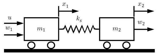
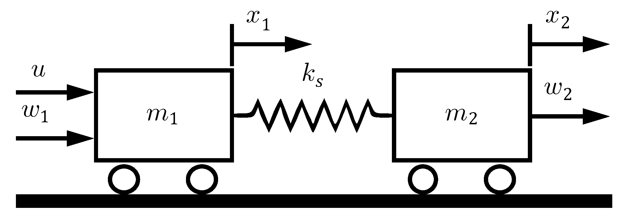
Consider the two-mass spring system [16,49] with friction-less sliding of Figure 1 where the masses $m_1$ with position $x_1$ and $m_2$ with position $x_2$ are linked by a spring with elastic constant $k_s$. The control input u is a force acting on $m_1$ and $w_1$ and $w_2$ are external disturbances acting on $m_1$ and $m_2$, respectively.

Figure 1. Two-mass spring system.

The system’s equations of motion using $x_3$ as the linear velocity of $m_1$ and $x_4$ as the linear velocity of $m_2$ are

$$\begin{array}{c}{\dot{x}}_1=x_3\\ {\dot{x}}_2=x_4\\ m_1{\dot{x}}_3=-k_s(x_1-x_2)+u+w_1\\ m_2{\dot{x}}_4=k_s(x_1-x_2)+w_2\end{array}$$

Setting the state vectors as $x={\left[x_1{x}_2{x}_3{x}_4\right]}^{\top }$ and additive disturbances as $w={\left[w_1{w}_2\right]}^{\top }$; its representation in the discrete state space by Euler’s approximation method, for a sampling time $T_{\mathrm{s}}$ is

$$\begin{array}{c}{x}_{k+1}=A{x}_k+B{u}_k+G{w}_k\\ A=\left[\begin{array}{cccc}1& 0& T_{\mathrm{s}}& 0\\ 0& 1& 0& T_{\mathrm{s}}\\ -\frac{k_s{T}_{\mathrm{s}}}{m_1}& \frac{k_s{T}_{\mathrm{s}}}{m_1}& 1& 0\\ \frac{k_s{T}_{\mathrm{s}}}{m_2}& -\frac{k_s{T}_{\mathrm{s}}}{m_2}& 0& 1\end{array}\right],B=\left[\begin{array}{c}0\\ 0\\ \frac{T_{\mathrm{s}}}{m_1}\\ 0\end{array}\right],G=\left[\begin{array}{cc}0& 0\\ 0& 0\\ \frac{T_{\mathrm{s}}}{m_1}& 0\\ 0& \frac{T_{\mathrm{s}}}{m_2}\end{array}\right]\end{array}$$

where $m_1,m_2=1$ kg are constant, $T_{\mathrm{s}}=0.1$ s (this was selected fulfilling the Nyquist–Shannon sampling theorem, taking the highest frequency of the poles of the system) and the constraints $|x_3|,|x_4|\le 0.12$ m/s must be satisfied. The elastic constant $k_s$ is associated with parametric uncertainties $\delta$ and it has a uniform probability distribution $k_s\sim \mathcal{U}\left([0.5,2.0]\right) \mathrm{N}/\mathrm{m}$. The additive disturbances w have a normal distribution $w\sim \mathcal{N}(0,{\mathsf{\Sigma }}_w) \mathrm{N}$ with zero mean and covariance matrix ${\mathsf{\Sigma }}_w=\mathrm{diag}({0.022}^2,{0.022}^2)$. For all controllers, when applying $N=6$, $Q_x=\mathrm{diag}(1,1,4,6)$, $R_u=1$; ${\epsilon }_{SMPC}=0.05$; ${\epsilon }_{SCMPC}=0.05$, ${\beta }_{SCMPC}={10}^{-9}$ and by means of (32), $M=896$.

Three cases were established based on the parameter $k_s$ to evaluate the performance of five MPCs (classic without constraints (MPC n/c), classic with constraints (MPC w/c), SMPC, SCMPC and Robust SCMPC):

• Case 1: $k_s$ is known, constant and it is set to its nominal value $k_s=1.25$.
• Case 2: $k_s$ is unknown and varies according to its probability distribution at every control period.
• Case 3: $k_s$ is unknown and remains constant for all instants along each simulation. The $k_s$ value varies according to its probability distribution in each simulation.

For each case, $N_{\mathrm{r}}=100$ simulations with $N_{T_{\mathrm{s}}}=100$ sampling times of duration were performed, starting from the initial state $x_{0|0}={\widehat{x}}_0={\left[0.50.500\right]}^{\top }$ towards the origin as the desired state.

For Case 1, the feedback matrix K and the terminal state weighting $P_N$ are obtained from solving a Quadratic Optimal Control Problem (LQR) [13,20]

$$K=\left[\begin{array}{cccc}\hfill -2.876& 1.683& -3.187\hfill & -0.904\end{array}\right],P_N=\left[\begin{array}{rrrr}\hfill 155.739& -102.335& 43.512\hfill & 77.451\\ \hfill -102.335& 117.489& -26.755\hfill & -30.134\\ \hfill 43.512& -26.755& 40.392\hfill & 15.371\\ \hfill 77.451& -30.134& 15.371\hfill & 126.794\end{array}\right]$$

For Cases 2 and 3, they are obtained by solving an eigenvalues problem (EVP); through a stability analysis of Lyapunov’s approach [13,32,33], such matrices are

$$K=\left[\begin{array}{cccc}\hfill -56.563& 41.356& -15.171\hfill & -45.156\end{array}\right],P_N=\left[\begin{array}{rrrr}\hfill 4509& -3280& 971\hfill & 3801\\ \hfill -3280& 2450& -709\hfill & -2706\\ \hfill 971& -709& 244\hfill & 791\\ \hfill 3801& -2706& 791\hfill & 3462\end{array}\right]$$

Case 1 Results: Table 2 shows high probabilities of success $p_{\mathrm{s}}$ ($0.84$, $0.74$ and $0.64$) by the stochastic MPCs. However, the biggest success of the SCMPC and Robust SCMPC required longer times $t_{\mathrm{avg}}$ ($79.0$ ms and $235.7$ ms) to obtain the control sequence than SMPC ($5.7$ ms), which works as a classic MPC with constraints. This makes sense since in each iteration SMPC and SCMPC select 896 random realizations for w and solve the OCP (30a) for all of them using (29) or (31).

Table 2. MPCs performance indices for Case 1.

MPC	${\mathit{N}}_{\mathbf{s}}$	${\mathit{p}}_{\mathbf{s}}$	${\mathit{N}}_{\mathbf{v}}$	${\mathbf{IAE}}_{\mathbf{avg}}$	${\mathbf{IAU}}_{\mathbf{avg}}$	${\mathit{t}}_{\mathbf{avg}}$	${\mathit{\sigma }}_{\mathbf{max}}$	${\mathbf{PO}}_{\mathbf{avg}}$
MPC n/c	0	$0.00$	2416	$43.88$	$5.35$	$5.6$ ms	$0.009$	$20.98\%$
MPC w/c	3	$0.03$	702	$49.01$	$7.29$	$5.9$ ms	$0.031$	$2.45\%$
SMPC	64	$0.64$	135	$49.85$	$7.39$	$5.7$ ms	$0.029$	$1.78\%$
SCMPC	84	$0.84$	168	$50.61$	$7.55$	$79.0$ ms	$0.036$	$6.78\%$
SCMPC (robust)	74	$0.74$	30	$52.50$	$8.70$	$235.7$ ms	$0.054$	$6.01\%$

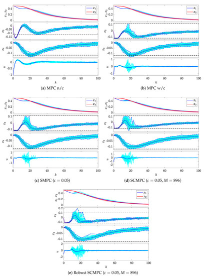
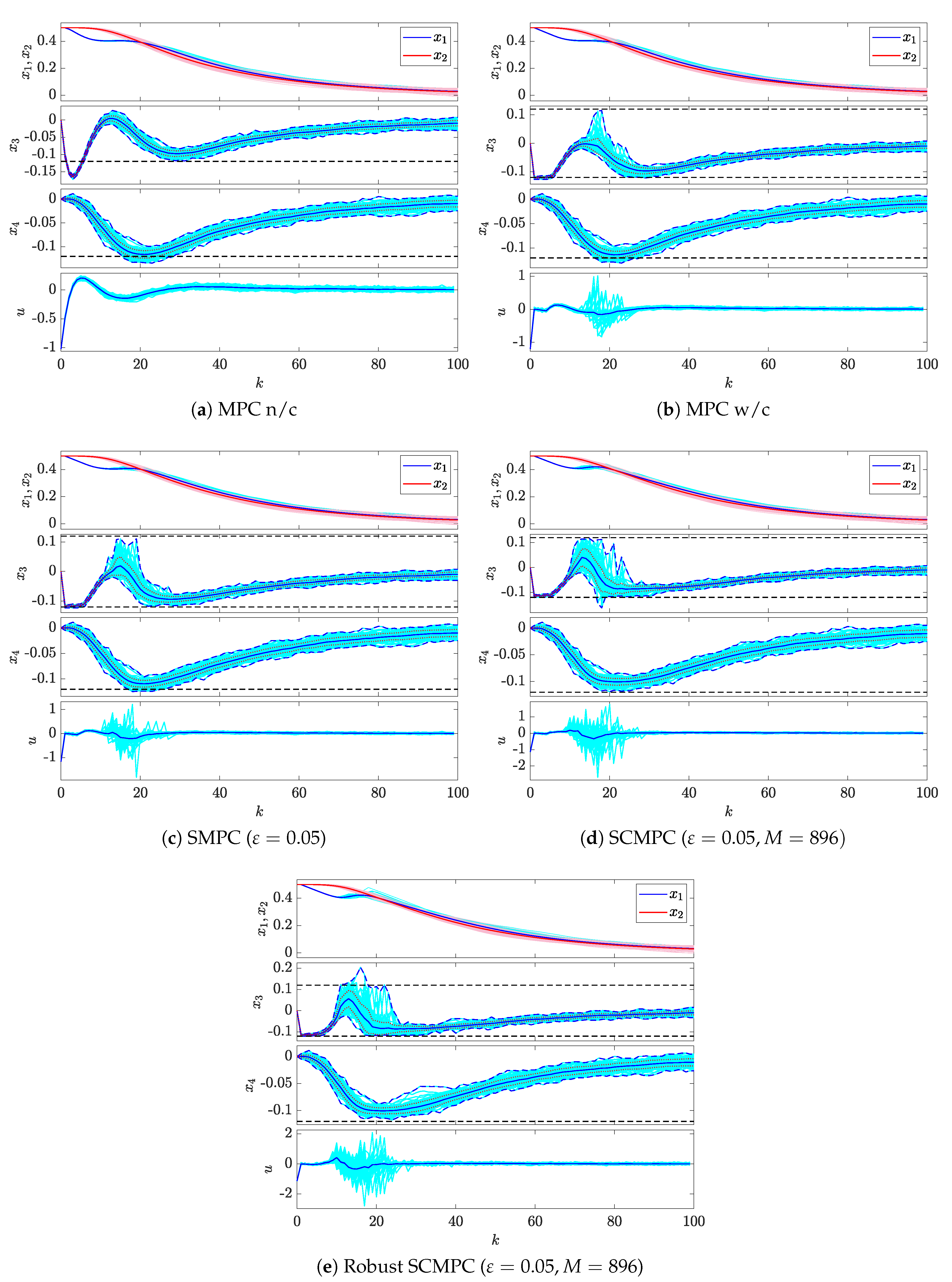
Figure 2 shows the $N_{\mathrm{r}}=100$ trajectories made by the real states and input (thin solid lines), starting from ${\widehat{x}}_0={\left[0.50.500\right]}^{\top }$ towards the origin. The MPC n/c (Figure 2a), having no constraints, presents the highest violations ($N_{\mathrm{v}}=2416$) and overshoots (${\mathrm{PO}}_{\mathrm{avg}}=20.98\%$), while the mean trajectories (thick solid lines) of the constrained MPCs do not exceed the limits (black dashed lines). Notice how stochastic approaches (Figure 2c–e) are within these limits or barely exceed them, showing that the probability that a state is within the allowed limits is $68\%$. The largest standard deviations ${\sigma }_{\max }$ occurred in the scenario-based MPCs ($0.036$ and $0.054$) due to the randomness mentioned in [29] and because the worst case is not always the closest to reality (hence, the highest IAE_avg ($52.50$) and IAU_avg ($8.70$) of all).

Figure 2. Case 1: Two-mass spring system controlled with different MPCs, for 100 Monte Carlo simulations. Trajectories of the real states and input (thin solid lines), mean value (thick solid lines), mean value with standard deviation (dotted lines), minimum and maximum values (blue dashed lines) and constraints (black dashed lines) $|x_3|,|x_4|\le 0.12$.

Case 2 Results: The performance indices and the real trajectories of the states are shown in Table 3 and Figure 3 respectively. As in Case 1, stochastic MPCs had the highest $p_{\mathrm{s}}$, observing an increase in the scenario-based schemes ($0.94$ and $0.86$), despite the randomness of $k_s$. Nevertheless, these schemes are the ones who take the longest to calculate the solution ($t_{\mathrm{avg}}$ ($220.3$ ms and $311.8$ ms) due to the fact that, in addition to selecting 896 random scenarios for w, it should also be done for $k_s$.

Table 3. MPCs performance indices: Case 2.

MPC	${\mathit{N}}_{\mathbf{s}}$	${\mathit{p}}_{\mathbf{s}}$	${\mathit{N}}_{\mathbf{v}}$	${\mathbf{IAE}}_{\mathbf{avg}}$	${\mathbf{IAU}}_{\mathbf{avg}}$	${\mathit{t}}_{\mathbf{avg}}$	${\mathit{\sigma }}_{\mathbf{max}}$	${\mathbf{PO}}_{\mathbf{avg}}$
MPC n/c	0	$0.00$	611	$50.58$	$6.16$	$6.3$ ms	$0.010$	$20.97\%$
MPC w/c	4	$0.04$	362	$51.37$	$5.59$	$6.4$ ms	$0.027$	$1.75\%$
SMPC	65	$0.65$	77	$51.98$	$5.87$	$6.3$ ms	$0.031$	$1.13\%$
SCMPC	94	$0.94$	7	$52.91$	$6.96$	$220.3$ ms	$0.045$	$13.67\%$
SCMPC (robust)	86	$0.86$	21	$53.14$	$8.70$	$311.8$ ms	$0.055$	$6.29\%$

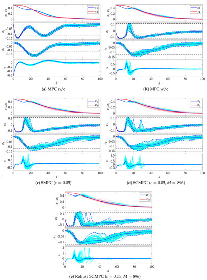
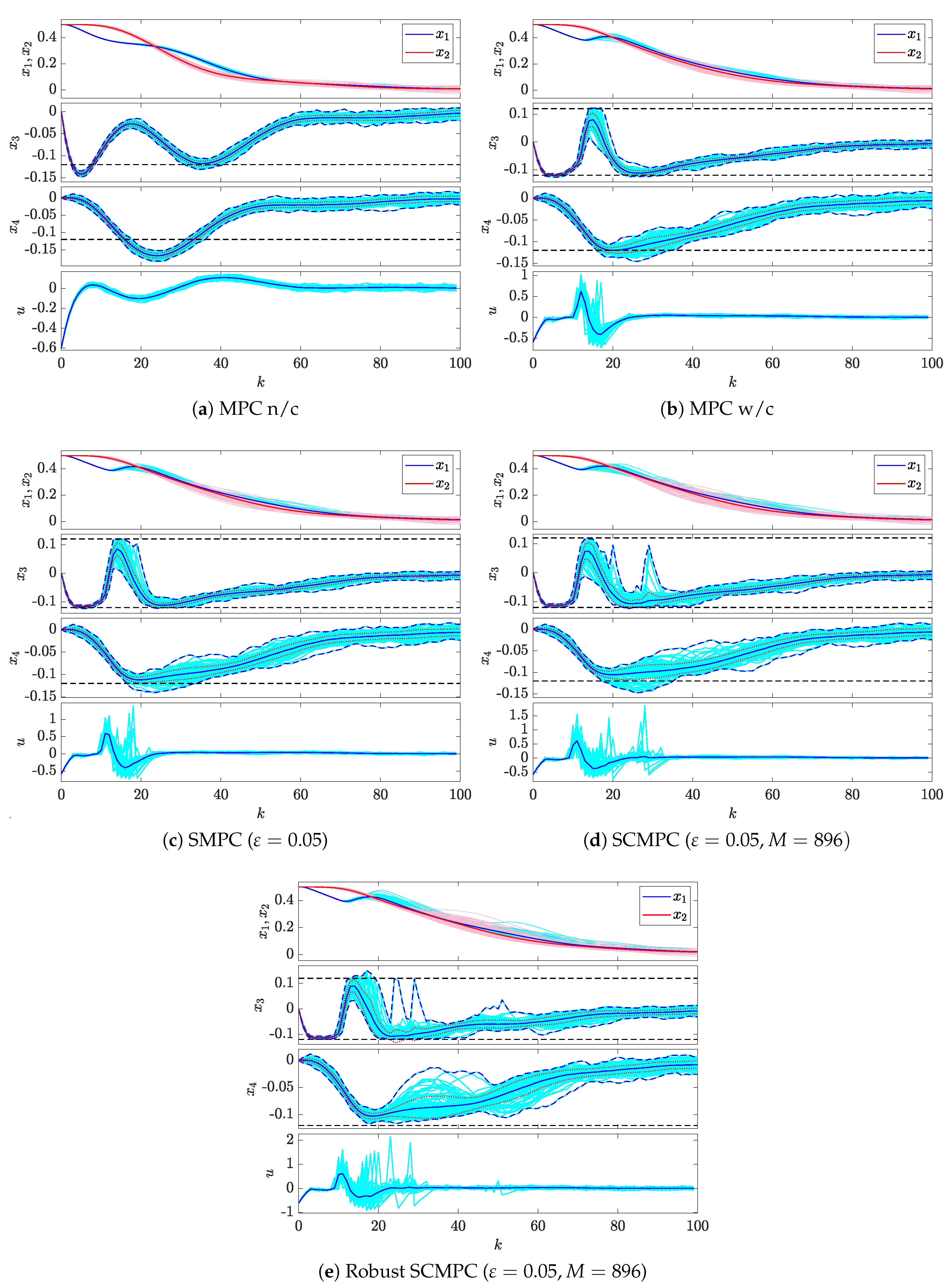
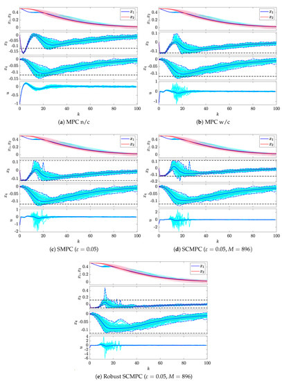
Figure 3. Case 2: Two-mass spring system controlled with different MPCs, for 100 Monte Carlo simulations. Trajectories of the real states and input (thin solid lines), mean value (thick solid lines), mean value with standard deviation (dotted lines), minimum and maximum values (blue dashed lines) and constraints (black dashed lines) $|x_3|,|x_4|\le 0.12$.

As seen in Figure 3, the mean trajectories that include the standard deviations of the stochastic MPCs are the only ones that stay within the limits (the probability that a state is within the allowed limits is $68\%$). This kind of robustness on stochastic strategies implies high values of IAE_avg and IAU_avg indicators compared to the others.

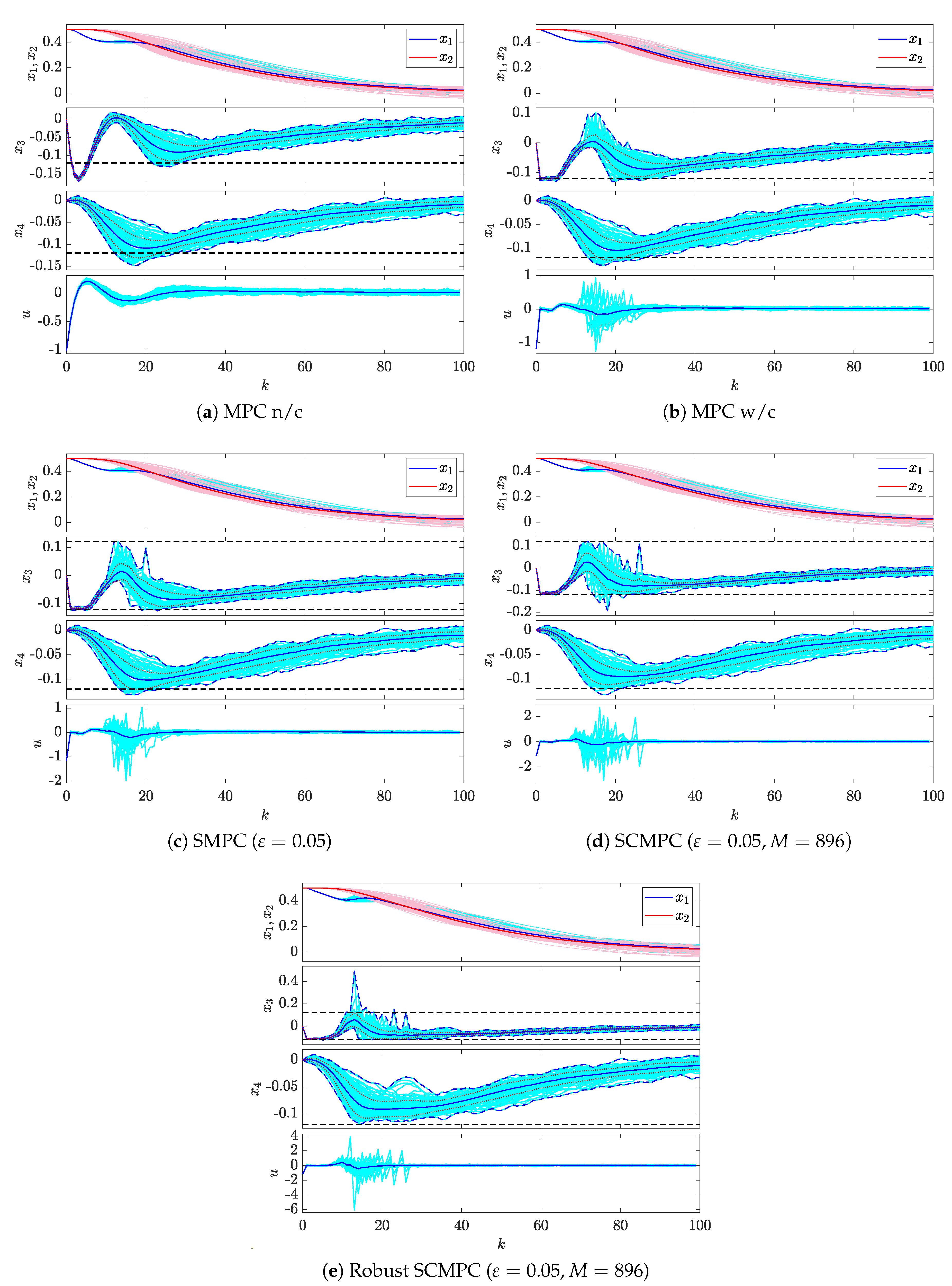
Case 3 Results: As can be seen in Table 4 and Figure 4, it is once again corroborated that the highest $p_{\mathrm{s}}$ and average trajectories with standard deviations within the limits belongs to stochastic MPCs. Regarding Case 2, the indicators $t_{\mathrm{avg}}$ are very similar, but for this case higher standard deviations ${\sigma }_{\max }$ of the three cases are observed. The high PO_avg ($28.23\%$) presented by the robust SCMPC can be seen in the trajectories of the $x_3$ (Figure 4e) state; however, this strategy presents the lowest $N_{\mathrm{v}}$ (27) of all MPCs.

Table 4. MPCs performance indices for Case 3.

MPC	${\mathit{N}}_{\mathbf{s}}$	${\mathit{p}}_{\mathbf{s}}$	${\mathit{N}}_{\mathbf{v}}$	${\mathbf{IAE}}_{\mathbf{avg}}$	${\mathbf{IAU}}_{\mathbf{avg}}$	${\mathit{t}}_{\mathbf{avg}}$	${\mathit{\sigma }}_{\mathbf{max}}$	${\mathbf{PO}}_{\mathbf{avg}}$
MPC n/c	0	$0.00$	754	$51.27$	$6.14$	$5.8$ ms	$0.028$	$19.38\%$
MPC w/c	1	$0.01$	462	$52.16$	$5.74$	$6.1$ ms	$0.032$	$2.07\%$
SMPC	57	$0.57$	107	$52.56$	$5.73$	$5.9$ ms	$0.036$	$1.90\%$
SCMPC	85	$0.85$	28	$53.42$	$6.95$	$220.9$ ms	$0.046$	$11.22\%$
SCMPC (robust)	79	$0.79$	27	$53.97$	$8.67$	$327.5$ ms	$0.062$	$28.23\%$

Figure 4. Case 3: Two-mass spring system controlled with different MPCs, for 100 Monte Carlo simulations. Trajectories of the real states and input (thin solid lines), mean value (thick solid lines), mean value with standard deviation (dotted lines), minimum and maximum values (blue dashed lines) and constraints (black dashed lines) $|x_3|,|x_4|\le 0.12$.

4.2. Example 2

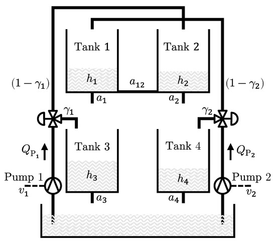
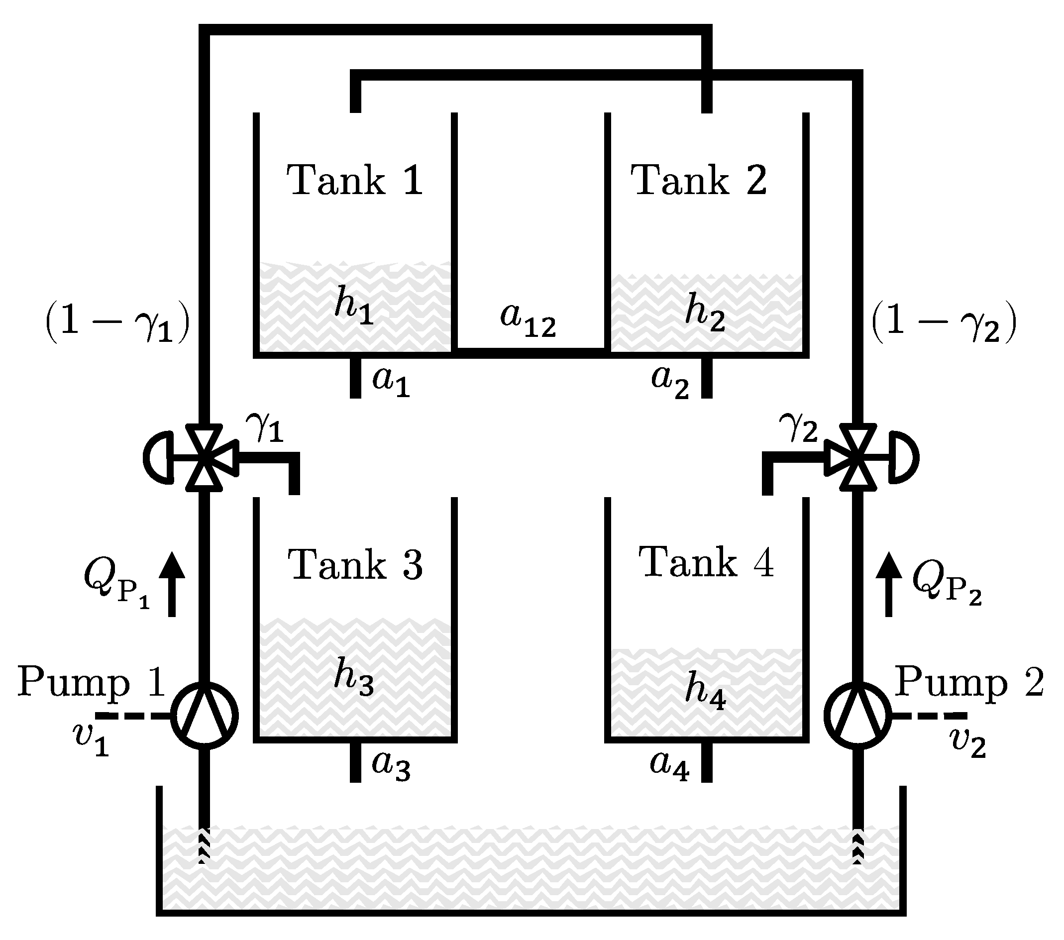
Consider the quadruple-tank system [50,51] of Figure 5, in which the aim is to control the level of liquid $h_i$ in tank i$\forall i\in \{1,2,3,4\}$, by means of pumps 1 and 2 whose flows are proportional to the applied voltage ($Q_{{\mathrm{P}}_1}=k_1{v}_1$, $Q_{{\mathrm{P}}_2}=k_2{v}_2$) and are distributed by the valves in proportions determined by ${\gamma }_1,{\gamma }_2\in [0,1]$.

Figure 5. Quadruple-tank system.

Let $A_i$ be the cross section of tank i; $a_i$ and $a_{12}$ are the areas of the tank outlet pipes; and g is the acceleration due to gravity. By performing a mass balance and applying Bernoulli’s law, the equations that describe the behavior of the nonlinear system are given by

$$\begin{array}{c}\frac{d{h}_1}{dt}=-\frac{a_1}{A_1}\sqrt{2g{h}_1}-\frac{a_{12}}{A_1}\mathrm{sgn}(h_1-h_2)\sqrt{2g|h_1-h_2|}+\frac{(1-{\gamma }_2)k_2}{A_1}{v}_2\\ \frac{d{h}_2}{dt}=-\frac{a_2}{A_2}\sqrt{2g{h}_2}+\frac{a_{12}}{A_2}\mathrm{sgn}(h_1-h_2)\sqrt{2g|h_1-h_2|}+\frac{(1-{\gamma }_1)k_1}{A_2}{v}_1\\ \frac{d{h}_3}{dt}=\frac{a_1}{A_3}\sqrt{2g{h}_1}-\frac{a_3}{A_3}\sqrt{2g{h}_3}+\frac{{\gamma }_1{k}_1}{A_3}{v}_1\\ \frac{d{h}_4}{dt}=\frac{a_2}{A_4}\sqrt{2g{h}_2}-\frac{a_4}{A_4}\sqrt{2g{h}_4}+\frac{{\gamma }_2{k}_2}{A_4}{v}_2\end{array}$$

(33)

Let us define the state vectors $x={\left[x_1{x}_2{x}_3{x}_4\right]}^{\top }$ and inputs $u={\left[u_1{u}_2\right]}^{\top }$; where $x_i=h_i-h_i^0$ and $u_i=v_i-v_i^0$ represent the deviations from the operating point $P^0=\{h_1^0,h_2^0,h_3^0,h_4^0,v_1^0,v_2^0\}=\{7.873\mathrm{cm},8.187\mathrm{cm},7.720\mathrm{cm},8.039\mathrm{cm},4.0\mathrm{V},3.5\mathrm{V}\}$. Linearizing around $P^0$ and using Euler’s approximation, for a sampling period $T_{\mathrm{s}}$, the linear model in the discrete state space can be represented by

$$\begin{array}{c}{x}_{k+1}=A{x}_k+B{u}_k\\ A=\left[\begin{array}{cccc}-\frac{{\beta }_1+{\beta }_x}{A_1}+1& \frac{{\beta }_x}{A_1}& 0& 0\\ \frac{{\beta }_x}{A_2}& -\frac{{\beta }_2+{\beta }_x}{A_2}+1& 0& 0\\ \frac{{\beta }_1}{A_3}& 0& -\frac{{\beta }_3}{A_3}+1& 0\\ 0& \frac{{\beta }_2}{A_4}& 0& -\frac{{\beta }_4}{A_4}+1\end{array}\right],B=\left[\begin{array}{cc}0& \frac{(1-{\gamma }_2)k_2}{A_1}{T}_{\mathrm{s}}\\ \frac{(1-{\gamma }_1)k_1}{A_2}{T}_{\mathrm{s}}& 0\\ \frac{{\gamma }_1{k}_1}{A_3}{T}_{\mathrm{s}}& 0\\ 0& \frac{{\gamma }_2{k}_2}{A_4}{T}_{\mathrm{s}}\end{array}\right]\\ \end{array}$$

where ${\beta }_i=a_i\sqrt{\frac{g}{2h_i^0}}{T}_{\mathrm{s}}$, ${\beta }_x=a_{12}\sqrt{\frac{g}{2|h_1^0-h_2^0|}}{T}_{\mathrm{s}}$; $A_i=144$ cm${}^2$, $a_1,a_2,a_{12}=0.352$ cm${}^2$, $a_3,a_4=1.006$ cm${}^2$; $k_1,k_2=33.333 {\mathrm{cm}}^3/\mathrm{Vs}$; ${\gamma }_1=0.6$, ${\gamma }_2=0.7$; $g=981 \mathrm{cm}/{\mathrm{s}}^2$, $T_{\mathrm{s}}=5$ s.

The constraints $|x_3|,|x_4|\le 1.5 \mathrm{cm}$, $|u_1|,|u_2|\le 1.0 \mathrm{V}$ must be satisfied and the process has additive disturbances w in its states, with normal distribution $w\sim \mathcal{N}(0,{\mathsf{\Sigma }}_w) \mathrm{cm}$ with zero mean and covariance matrix ${\mathsf{\Sigma }}_w=\mathrm{diag}({0.1}^2,{0.1}^2,{0.1}^2,{0.1}^2)$, which are truncated $|w_i|\le 0.3 \mathrm{cm}$ and $G=\mathrm{diag}(1,1,1,1)$.

To analyze the effect of the allowed violation probabilities in the states, $\epsilon$, on the number of considered scenarios M and on the different performance indicators, this example compares the performance of an SCMPC for five values of $\epsilon (0.4,0.3,0.2,0.1,0.05)$ with a constrained classic MPC (MPC w/c). For each scheme, $N_{\mathrm{r}}=100$ runs were carried out on the nonlinear model (33), each one with $N_{T_{\mathrm{s}}}=40$ sampling times of duration, starting from the initial state $x_{0|0}={\widehat{x}}_0={[-5.5-6.9-0.5-0.2]}^{\top }$ towards the origin as the desired state.

For all controllers, $N=5$, $Q_x=\mathrm{diag}(10,10,1,1)$, $R_u=\mathrm{diag}(1,1)$, $\beta ={10}^{-9}$. The matrices K and $P_N$, obtained from solving a Quadratic Optimal Control Problem (LQR) [13,20], are

$$K=\left[\begin{array}{cccc}\hfill -0.745& -0.649& -0.153\hfill & 0.054\\ \hfill -0.556& -0.662& 0.045\hfill & -0.245\end{array}\right],P_N=\left[\begin{array}{cccc}\hfill 13.275& 3.341& -0.839\hfill & -0.811\\ \hfill 3.341& 13.438& -0.884\hfill & -0.809\\ \hfill -0.839& -0.884& 1.870\hfill & 0.140\\ \hfill -0.811& -0.809& 0.140\hfill & 1.689\end{array}\right]$$

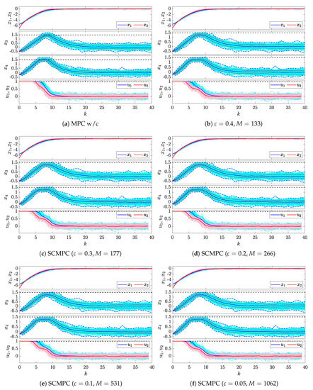
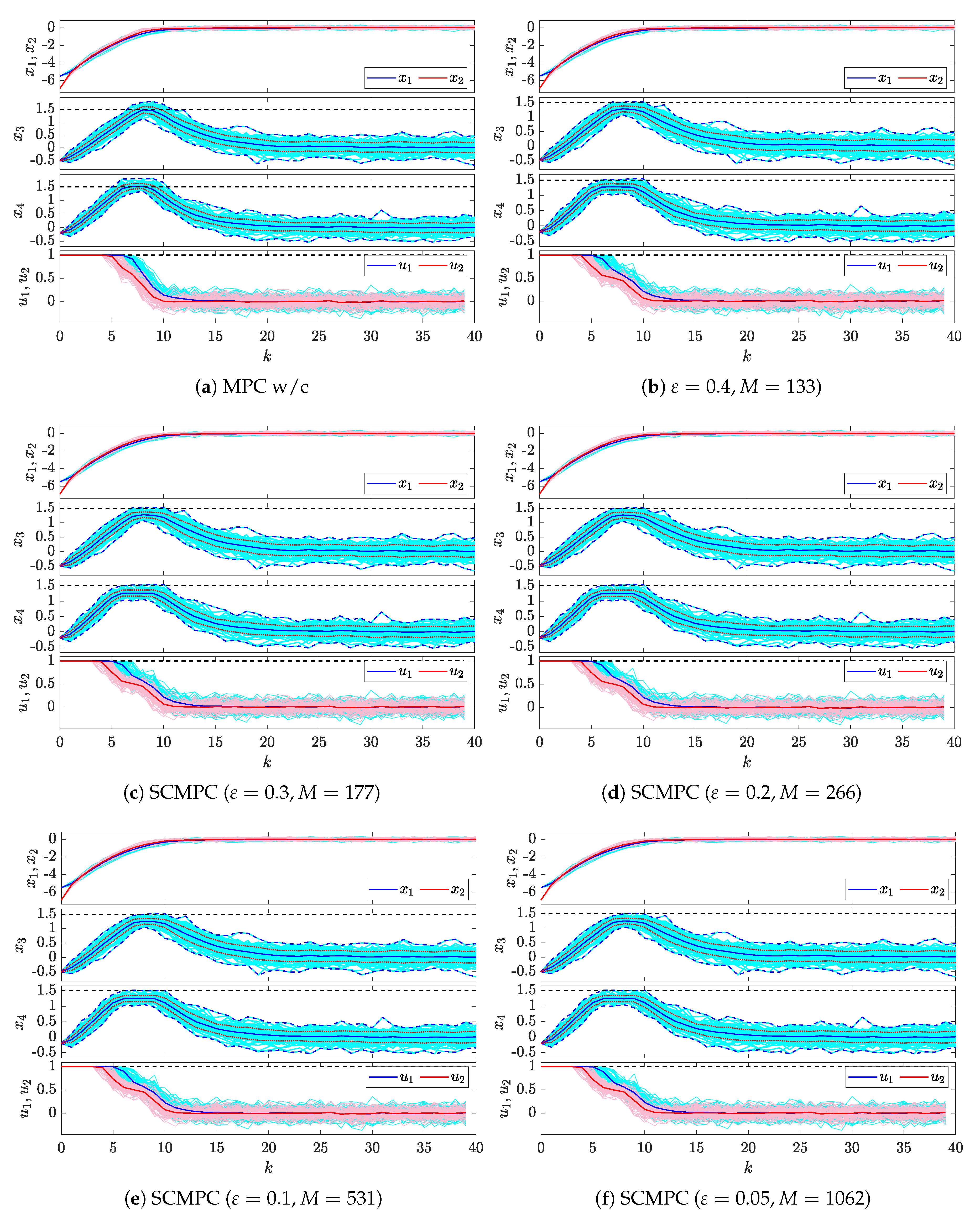
Results: Table 5 shows the performance indices of the MPC w/c and the SCMPC, for the $N_{\mathrm{r}}=100$ runs, while Figure 6 depicts the closed loop simulations. SCMPCs showed the lowest violations, in both quantity $N_{\mathrm{v}}$ ($15,14,10,7$ and 6) and percentage of deviation ${\mathrm{PO}}_{\mathrm{avg}}$ ($1.55\%,1.60\%,1.78\%,1.06\%$ and $0.48\%$) compared to the MPC w/c ($N_{\mathrm{v}}=263$ and ${\mathrm{PO}}_{\mathrm{avg}}=5.76\%$). Furthermore, the stochastic scheme shows high values of successful runs $N_{\mathrm{s}}$ ($87,88,91,93$ and 94) and probabilities of success $p_{\mathrm{s}}$ ($0.87,0.88,0.91,0.93$ and $0.94$), which increase as $\epsilon$ decreases. However, this improvement in $p_{\mathrm{s}}$ leads to an increase in the number of scenarios M ($133,177,266,531$ and 1062) to be considered in the OCP (30a), and hence an increase in the average time that the algorithm takes to find a solution at each instant k ($t_{\mathrm{avg}}$ ($12.3\mathrm{ms},14.2\mathrm{ms},18.1\mathrm{ms}$ and $30.3$ ms). Regarding the indices ${\mathrm{IAE}}_{\mathrm{avg}}$, ${\mathrm{IAU}}_{\mathrm{avg}}$ and ${\sigma }_{\max }$, despite not observing a considerable difference between controllers, it can be concluded that the lower the $\epsilon$ the lower the performance values.

Table 5. Performance indices.

MPC	${\mathit{N}}_{\mathbf{s}}$	${\mathit{p}}_{\mathbf{s}}$	${\mathit{N}}_{\mathbf{v}}$	${\mathbf{IAE}}_{\mathbf{avg}}$	${\mathbf{IAU}}_{\mathbf{avg}}$	${\mathit{t}}_{\mathbf{avg}}$	${\mathit{\sigma }}_{\mathbf{max}}$	${\mathbf{PO}}_{\mathbf{avg}}$
MPC w/c	2	$0.02$	263	$78.63$	$21.51$	$6.7$ ms	$0.218$	$5.76\%$
SCMPC $\left(\begin{array}{c}\epsilon =0.4\\ M=133\end{array}\right)$	87	$0.87$	15	$78.40$	$21.22$	$12.3$ ms	$0.218$	$1.55\%$
SCMPC $\left(\begin{array}{c}\epsilon =0.3\\ M=177\end{array}\right)$	88	$0.88$	14	$78.39$	$21.21$	$14.2$ ms	$0.218$	$1.60\%$
SCMPC $\left(\begin{array}{c}\epsilon =0.2\\ M=266\end{array}\right)$	91	$0.91$	10	$78.38$	$21.18$	$18.1$ ms	$0.218$	$1.78\%$
SCMPC $\left(\begin{array}{c}\epsilon =0.1\\ M=531\end{array}\right)$	93	$0.93$	7	$78.36$	$21.15$	$30.3$ ms	$0.217$	$1.06\%$
SCMPC $\left(\begin{array}{c}\epsilon =0.05\\ M=1062\end{array}\right)$	94	$0.94$	6	$78.35$	$21.14$	$57.3$ ms	$0.217$	$0.48\%$

Figure 6. Quadruple-tank system controlled with a constrained MPC and a SCMPC for multiple $\epsilon$ values, for 100 Monte Carlo simulations. Trajectories of the real states and inputs (thin solid lines), mean value (thick solid lines), mean value with standard deviation (dotted lines), minimum and maximum values (blue dashed lines) and constraints (black dashed lines) $|x_3|,|x_4|\le 1.5$, $|u_1|,|u_2|\le 1.0$.

As can be seen in the Figure 6, all the $N_{\mathrm{r}}=100$ trajectories made by the states (thin solid lines) start from $N_{\mathrm{r}}=100$ towards the origin, where the mean trajectories (thick solid lines) of the SCMPCs are considerably far from the constraints (black dashed lines), opposite to that of the MPC w/c that passes very close and even violates them (that’s why the highest ${\mathrm{PO}}_{\mathrm{avg}}=5.76\%$ of them). On the other hand, for SCMPCs, the average trajectories that include the standard deviations (dashed lines) are within the limits. It means that the probability that a state is within the allowed limits is $68\%$. As for the applied inputs, they start at their maximum allowed values and decrease as the states converge towards the origin

5. Conclusions and Future Work

Two stochastic predictive control approaches are compared in this article; one based on analytical methods (SMPC) and the other based on scenarios (SCMPC). The low computational cost of the SMPC is because the uncertain statistical information is used offline to adjust the states constraints. However, if this information changes, it cannot be considered during operation. On the other hand, this new statistical information can be incorporated into the SCMPC to generate the scenarios online, but it leads to a high computational cost.

It is shown that the SMPC can be summed up in a deterministic OCP (22a) whose structure is similar to that of a classic MPC with constraints (7a), with similar computational cost $t_{\mathrm{avg}}$, but with a considerable increase in the probability of success $p_{\mathrm{s}}$, due to offline constraint adjustment.

Scenario-based approaches SCMPC and robust SCMPC, compared to the others, gave the highest probabilities of success, at the expense of a high computational cost, since they need to solve an OCP with M random scenarios for each control period. From results shown in Table 5, can be concluded that a decrease in the parameter $\epsilon$, related to the probability of violation allowed for the state constraints, produces an increase in the probability of success $p_{\mathrm{s}}$. However, this improvement results in an increase in the number of M scenarios to be considered in the OCP and therefore an increase in the average time $t_{\mathrm{avg}}$ that the algorithm takes to find a solution at each sampling time.

It is clear that the consideration of statistical process information, through its inclusion in the OCP, significantly improves the probability of success $p_{\mathrm{s}}$. This can be verified in Figure 2, Figure 3, Figure 4 and Figure 6, where it is observed that only stochastic approaches reached mean trajectories with standard deviations within the limits or barely exceeding them. Thus, for a normal distribution, it means that the probability a state is within the allowed limits is $68\%$.

Scenario-based schemes are attractive in the sense that they have a greater probability of success and the inclusion of new statistical information online without necessarily known probability distributions. However, due to the randomness of scenarios, their solution can show undesirable behaviors despite their high computational cost. This drawbacks would prevent their implementation for the control of systems with fast dynamics such as the two-mass spring system in the example, which has $T_{\mathrm{s}}$ ($0.1$ s) close to the lowest $t_{\mathrm{avg}}$ ($79.0$ ms) of the SCMPCs of the three cases. Given these drawbacks, future work continues on the proposal of new SCMPC schemes that reduce the computational load and unlikely scenarios.

Finally, the specialized software Stochastic Model Predictive Control Toolbox is available in MATLAB Central for the keen readers. This tool was created by the authors to carry out part of the simulations in this article. It also allows readers to reproduce the results here presented or to tune and simulate SMPCs or SCMPCs for controlling multivariable systems with additive disturbances which present Gaussian probability distributions.

References

- Richalet, J.; Rault, A.; Testud, J.; Papon, J. Model predictive heuristic control: Applications to industrial processes. Automatica 1978, 14, 413–428. [Google Scholar] [CrossRef] [Scilit]
- Forbes, M.G.; Patwardhan, R.S.; Hamadah, H.; Gopaluni, R.B. Model Predictive Control in Industry: Challenges and Opportunities. IFAC Pap. 2015, 48, 531–538. [Google Scholar] [CrossRef] [Scilit]
- Jurado, I.; Millán, P.; Quevedo, D.; Rubio, F. Stochastic MPC with Applications to Process Control. Int. J. Control 2014, 88, 792–800. [Google Scholar] [CrossRef] [Scilit]
- Richalet, J.; Abu El Ata-Doss, S.; Arber, C.; Kuntze, H.; Jacubasch, A.; Schill, W. Predictive Functional Control-Application to Fast and Accurate Robots. IFAC Proc. Vol. 1987, 20, 251–258. [Google Scholar] [CrossRef] [Scilit]
- Tan, Y.; Cai, G.; Li, B.; Teo, K.L.; Wang, S. Stochastic Model Predictive Control for the Set Point Tracking of Unmanned Surface Vehicles. IEEE Access 2020, 8, 579–588. [Google Scholar] [CrossRef] [Scilit]
- Mueller, M.W.; D’Andrea, R. A model predictive controller for quadrocopter state interception. In Proceedings of the 2013 European Control Conference (ECC), Zurich, Switzerland, 17–19 July 2013; pp. 1383–1389. [Google Scholar] [CrossRef] [Scilit]
- Lamoudi, M.Y.; Alamir, M.; Béguery, P. Model predictive control for energy management in buildings Part 2: Distributed Model Predictive Control. IFAC Proc. Vol. 2012, 45, 226–231. [Google Scholar] [CrossRef] [Scilit]
- Salsbury, T.; Mhaskar, P.; Qin, S.J. Predictive control methods to improve energy efficiency and reduce demand in buildings. Comput. Chem. Eng. 2013, 51, 77–85. [Google Scholar] [CrossRef] [Scilit]
- Sultana, W.R.; Sahoo, S.K.; Sukchai, S.; Yamuna, S.; Venkatesh, D. A review on state-of-the-art development of model predictive control for renewable energy applications. Renew. Sustain. Energy Rev. 2017, 76, 391–406. [Google Scholar] [CrossRef] [Scilit]
- Luchini, E.; Schirrer, A.; Kozek, M. A hierarchical MPC for multi-objective mixed-integer optimisation applied to redundant refrigeration circuits. IFAC Pap. 2017, 50, 9058–9064. [Google Scholar] [CrossRef] [Scilit]
- Mercorelli, P.; Kubasiak, N.; Liu, S. Model predictive control of an electromagnetic actuator fed by multilevel PWM inverter. In Proceedings of the 2004 IEEE International Symposium on Industrial Electronics, Ajaccio, France, 4–7 May 2004; pp. 531–535. [Google Scholar] [CrossRef] [Scilit]
- Mayne, D.; Rawlings, J.; Rao, C.; Scokaert, P. Constrained Model Predictive Control: Stability and Optimality. Automatica 2000, 36, 789–814. [Google Scholar] [CrossRef] [Scilit]
- Maciejowski, J. Predictive Control: With Constraints, 1st ed.; Prentice Hall: London, UK, 2002. [Google Scholar]
- Kouvaritakis, B.; Cannon, M. Model Predictive Control. Classical, Robust and Stochastic, 1st ed.; Springer International Publishing: London, UK, 2016. [Google Scholar] [CrossRef] [Scilit]
- Mayne, D.Q. Model Predictive Control: Recent Developments and Future Promise. Automatica 2014, 50, 2967–2986. [Google Scholar] [CrossRef] [Scilit]
- Kothare, M.V.; Balakrishnan, V.; Morari, M. Robust Constrained Model Predictive Control Using Linear Matrix Inequalities. Automatica 1996, 32, 1361–1379. [Google Scholar] [CrossRef] [Scilit]
- Bemporad, A.; Morari, M. Robust Model Predictive Control: A Survey. In Robustness in Identification and Control; Springer: London, UK, 1999; pp. 207–226. [Google Scholar] [CrossRef] [Scilit]
- Mesbah, A. Stochastic Model Predictive Control: An Overview and Perspectives for Future Research. IEEE Control Syst. Mag. 2016, 36, 30–44. [Google Scholar] [CrossRef] [Scilit]
- Mayne, D. Robust and Stochastic MPC: Are We Going in the Right Direction? IFAC Pap. 2015, 48, 1–8. [Google Scholar] [CrossRef] [Scilit]
- Kouvaritakis, B.; Cannon, M. Stochastic Model Predictive Control. In Encyclopedia of Systems and Control, 1st ed.; Springer: London, UK, 2015; pp. 1350–1357. [Google Scholar] [CrossRef] [Scilit]
- Farina, M.; Giulioni, L.; Scattolini, R. Stochastic Linear Model Predictive Control with Chance Constraints—A Review. J. Process. Control 2016, 44, 53–67. [Google Scholar] [CrossRef] [Scilit]
- Hewing, L.; Zeilinger, M.N. Scenario-Based Probabilistic Reachable Sets for Recursively Feasible Stochastic Model Predictive Control. IEEE Control Syst. Lett. 2020, 4, 450–455. [Google Scholar] [CrossRef] [Scilit]
- Cannon, M.; Kouvaritakis, B.; Raković, S.V.; Cheng, Q. Stochastic Tubes in Model Predictive Control With Probabilistic Constraints. IEEE Trans. Autom. Control 2011, 56, 194–200. [Google Scholar] [CrossRef] [Scilit]
- Lorenzen, M.; Dabbene, F.; Tempo, R.; Allgöwer, F. Constraint-Tightening and Stability in Stochastic Model Predictive Control. IEEE Trans. Autom. Control 2017, 62, 3165–3177. [Google Scholar] [CrossRef] [Scilit]
- Heirung, T.A.N.; Paulson, J.A.; O’Leary, J.; Mesbah, A. Stochastic Model Mredictive Control-How Does It Work? Comput. Chem. Eng. 2018, 114, 158–170. [Google Scholar] [CrossRef] [Scilit]
- Paulson, J.A.; Buehler, E.A.; Braatz, R.D.; Mesbah, A. Stochastic Model Predictive Control with Joint Chance Constraints. Int. J. Control 2017, 93, 126–139. [Google Scholar] [CrossRef] [Scilit]
- Mayne, D.Q.; Falugi, P. Stabilizing Conditions for Model Predictive Control. Int. J. Robust Nonlinear Control 2018, 29, 894–903. [Google Scholar] [CrossRef] [Scilit]
- Calafiore, G.C.; Fagiano, L. Robust Model Predictive Control Via Scenario Optimization. IEEE Trans. Autom. Control 2013, 58, 219–224. [Google Scholar] [CrossRef] [Scilit]
- Schildbach, G.; Fagiano, L.; Frei, C.; Morari, M. The Scenario Approach for Stochastic Model Predictive Control with Bounds on Closed-Loop Constraint Violations. Automatica 2014, 50, 3009–3018. [Google Scholar] [CrossRef] [Scilit]
- Calafiore, G.; Campi, M.C. The Scenario Approach to Robust Control Design. IEEE Trans. Autom. Control 2006, 51, 742–753. [Google Scholar] [CrossRef] [Scilit]
- González Querubín, E.A. Stochastic Model Predictive Control Toolbox. Version 1.0.4. Available online: https://www.mathworks.com/matlabcentral/fileexchange/75803 (accessed on 5 December 2020).
- Boyd, S.; El Ghaoui, L.; Feron, E.; Balakrishnan, V. Linear Matrix Inequalities in System and Control Theory; Society for Industrial and Applied Mathematics: Philadelphia, PA, USA, 1994. [Google Scholar] [CrossRef] [Scilit]
- Cuzzola, F.A.; Geromel, J.C.; Morari, M. An Improved Approach for Constrained Robust Model Predictive Control. Automatica 2002, 38, 1183–1189. [Google Scholar] [CrossRef] [Scilit]
- Maeder, U.; Borrelli, F.; Morari, M. Linear Offset-Free Model Predictive Control. Automatica 2009, 45, 2214–2222. [Google Scholar] [CrossRef] [Scilit]
- Blanchini, F.; Miani, S. Set-Theoretic Methods in Control, 1st ed.; Birkhäuser Boston: Boston, MA, USA, 2008. [Google Scholar] [CrossRef] [Scilit]
- Khlebnikov, M.V.; Polyak, B.T.; Kuntsevich, V.M. Optimization of Linear Systems Subject to Bounded Exogenous Disturbances: The Invariant Ellipsoid Technique. Autom. Remote. Control 2011, 72, 2227–2275. [Google Scholar] [CrossRef] [Scilit]
- Zhang, X.; Grammatico, S.; Schildbach, G.; Goulart, P.; Lygeros, J. On the Sample Size of Randomized MPC for Chance-Constrained Systems with Application to Building Climate Control. In Proceedings of the 2014 European Control Conference (ECC), Strasbourg, France, 24–27 June 2014; pp. 478–483. [Google Scholar] [CrossRef] [Scilit]
- Parisio, A.; Varagnolo, D.; Molinari, M.; Pattarello, G.; Fabietti, L.; Johansson, K.H. Implementation of a Scenario-based MPC for HVAC Systems: An Experimental Case Study. IFAC Proc. Vol. 2014, 47, 599–605. [Google Scholar] [CrossRef] [Scilit]
- Wang, X.; Liu, Y.; Xu, L.; Liu, J.; Sun, H. A Chance-Constrained Stochastic Model Predictive Control for Building Integrated with Renewable Resources. Electr. Power Syst. Res. 2020, 184, 106348. [Google Scholar] [CrossRef] [Scilit]
- Raimondi Cominesi, S.; Farina, M.; Giulioni, L.; Picasso, B.; Scattolini, R. A Two-Layer Stochastic Model Predictive Control Scheme for Microgrids. IEEE Trans. Control Syst. Technol. 2018, 26, 1–13. [Google Scholar] [CrossRef] [Scilit]
- Ramandi, M.Y.; Bigdeli, N.; Afshar, K. Stochastic Economic Model Predictive Control for Real-Time Scheduling of Balance Responsible Parties. Int. J. Electr. Power Energy Syst. 2020, 118, 105800. [Google Scholar] [CrossRef] [Scilit]
- Velarde, P.; Tian, X.; Sadowska, A.D.; Maestre, J.M. Scenario-Based Hierarchical and Distributed MPC for Water Resources Management with Dynamical Uncertainty. Water Resour. Manag. 2018, 33, 677–696. [Google Scholar] [CrossRef] [Scilit]
- Velasco, J.; Liniger, A.; Zhang, X.; Lygeros, J. Efficient Implementation of Randomized MPC for Miniature Race Cars. In Proceedings of the 2016 European Control Conference (ECC), Aalborg, Denmark, 29 June 2016; pp. 957–962. [Google Scholar] [CrossRef] [Scilit]
- Piovesan, J.L.; Tanner, H.G. Randomized Model Predictive Control for Robot Navigation. In Proceedings of the 2009 IEEE International Conference on Robotics and Automation, Kobe, Japan, 17 May 2009; pp. 94–99. [Google Scholar] [CrossRef] [Scilit]
- Goodwin, G.C.; Medioli, A.M. Scenario-Based, Closed-Loop Model Predictive Control With Application to Emergency Vehicle Scheduling. Int. J. Control 2013, 86, 1338–1348. [Google Scholar] [CrossRef] [Scilit]
- Mesbah, A. Stochastic Model Predictive Control with Active Uncertainty Learning: A Survey on Dual Control. Annu. Rev. Control 2018, 45, 107–117. [Google Scholar] [CrossRef] [Scilit]
- Cannon, M.; Kouvaritakis, B.; Ng, D. Probabilistic Tubes in Linear Stochastic Model Predictive Control. Syst. Control Lett. 2009, 58, 747–753. [Google Scholar] [CrossRef] [Scilit]
- Calafiore, G.C. Random Convex Programs. SIAM J. Optim. 2010, 20, 3427–3464. [Google Scholar] [CrossRef] [Scilit]
- Wie, B.; Bernstein, D.S. Benchmark Problems for Robust Control Design. J. Guid. Control Dyn. 1992, 15, 1057–1059. [Google Scholar] [CrossRef] [Scilit]
- Johansson, K.H.; Polyak, B.T.; Kuntsevich, V.M. The Quadruple-Tank Process: A Multivariable Laboratory Process With an Adjustable Zero. IEEE Trans. Control Syst. Technol. 2000, 8, 456–465. [Google Scholar] [CrossRef] [Scilit]
- Numsomran, A.; Tipsuwanporn, V.; Tirasesth, K. Modeling of the Modified Quadruple-Tank Process. In Proceedings of the 2008 SICE Annual Conference, Tokyo, Japan, 20–22 August 2008; pp. 818–823. [Google Scholar] [CrossRef] [Scilit]
Publisher’s Note: MDPI stays neutral with regard to jurisdictional claims in published maps and institutional affiliations. |
© 2020 by the authors. Licensee MDPI, Basel, Switzerland. This article is an open access article distributed under the terms and conditions of the Creative Commons Attribution (CC BY) license (http://creativecommons.org/licenses/by/4.0/).