


Abstract
Unmanned aerial vehicles (UAVs) for urban and clinical–logistics missions operate under severe constraints in onboard energy, computation, and payload integrity. Addressing these challenges requires not only advanced algorithms but also a tight integration between embedded hardware, energy management, perception, and decision-making. This paper presents a unified UAV platform based on a system-level hardware–software co-design. First, a compact six-layer PCB (85 mm × 55 mm) integrates an NVIDIA Jetson Orin for on-edge artificial intelligence and a dedicated microcontroller for real-time flight control, with explicit power-domain separation, thermal management via arrays, and physical isolation of sensitive sensors. Second, a hybrid energy system combines LiPo batteries with perovskite photovoltaic cells and an MPPT stage with experimentally measured efficiency (94.5%), enabling stable operation under variable irradiance conditions. Third, an autonomous navigation strategy based on a Dueling Double Deep Q Network with Prioritized Experience Replay learns energy-efficient trajectories while explicitly incorporating payload thermal deviation (ΔT) and mechanical jerk into the reward function, thereby supporting clinically safe transport. Experimental validation on the physical platform includes onboard power and latency measurements, statistical evaluation across training and deterministic execution, and mission-level key performance indicators. Results show an average reduction of 18.4% in total energy consumption and a 12.1% increase in operational coverage under representative urban scenarios, with end-to-end decision latency below 50 ms. These findings demonstrate that a tightly integrated design of embedded hardware, hybrid energy management, and clinical-aware reinforcement learning enables robust, efficient, and application-ready UAV systems for urban and healthcare missions.
Keywords:
UAV; embedded AI; power management; energy harvesting; DQN; PCB miniaturization; LiPo; BLDC; perovskite PV; urban monitoring 1. Introduction
The development of unmanned aerial systems in recent years has made UAVs an increasingly essential part of smart mobility strategies, urban logistics, and territorial monitoring applications. The ability of drones to avoid traffic, quickly access hard-to-reach areas, and operate with zero local emissions makes them especially suitable for supporting light delivery systems, healthcare networks, and real-time observation tasks. Recent studies highlight that, in complex urban environments, UAVs offer significant operational benefits in terms of speed, flexibility, and environmental sustainability, helping reduce energy consumption and lower carbon footprints compared to traditional transportation methods [1]. At the same time, the expansion of high-efficiency electrical technologies is advancing platform development, with brushless motors, high-capacity batteries, and increasingly lightweight, high-performance materials [2].
In the healthcare industry, “medical drone logistics” has shown particular potential for the time-sensitive transport of biological samples, blood products, and cold-chain medicines, where faster transit times offer clinical benefits and reduce staff exposure during emergencies. Positive results have been achieved when UAV fleets are coordinated with event-driven workflows, multi-objective planning, and GIS integration to manage bases, corridors, and delivery points, as well as to monitor urban traffic flow. In such clinical–urban missions, along with energy and safety constraints, thermo-mechanical limitations (ΔT on payload, jerk/vibrations) and navigation reliability requirements become essential, demanding planning strategies that balance performance, transport quality, and operational rules within the urban environment [1,3,4,5].
Despite these prospects, the systematic use of drones in real urban environments still faces structural, energy, and operational challenges. Specifically, missions in “urban canyons” are affected by turbulence, GNSS interference, and dense obstacles, making navigation strategies that rely solely on GPS or basic avoidance algorithms unreliable [3]. The built environment causes sudden changes in wind direction, pressure gradients, and local vortices, significantly increasing energy consumption and requiring dynamic, reactive flight control. If these effects are not properly addressed, they can greatly reduce UAV autonomy, worsening one of the sector’s main issues: limited battery capacity, which remains a key obstacle to frequent and medium-range operations [6].
At the same time, increasing interest in hybrid energy solutions has driven the development of solar drones powered by lightweight, high-efficiency photovoltaic cells. Perovskite-based technologies, in particular, show promising potential for extending flight time due to their high specific efficiency and ability to be integrated onto curved or irregular surfaces [7,8]. However, the latest studies agree that, while improving the overall energy balance, the photovoltaic contribution is significant only if it is part of a comprehensive energy management system capable of balancing power demand, solar generation, and battery charging in real time [9]. Without adaptive logic, solar harvesting tends to provide minimal benefits, especially under variable operating conditions [7,9].
On the algorithmic front, integrating artificial intelligence models into autonomous UAV navigation is becoming increasingly crucial. Techniques based on Deep Reinforcement Learning (DRL), especially variants of Deep Q-Network (DQN), have been demonstrated to improve drone decision-making in complex environments, enabling more robust, adaptable, and environmentally aware flight strategies [10,11]. The use of these methods has been particularly effective in the presence of atmospheric disturbances, dynamic obstacles, or operating conditions that are not fully known. However, applying such algorithms on embedded platforms remains challenging due to limited computational resources and latency constraints imposed by flight control [4,11].
The literature shows that many studies focus on high-computational-power simulations or on subsystem designs treated independently: trajectory optimizations often ignore realistic energy models; consumption models do not account for complex aerodynamic phenomena; sensory fusion strategies do not communicate effectively with navigation models [10]. Similarly, research on solar drones tends to emphasize photovoltaics, neglecting the need to integrate them into a broader mission cycle that connects aerodynamics, communication, and computation [7,9].
It is important to clarify that several components adopted in this work are based on well-established methods widely reported in the literature. Specifically, the fusion of GNSS, IMU, and LiDAR measurements relies on the standard Extended Kalman Filter formulations; photovoltaic energy harvesting is managed through conventional MPPT strategies; and autonomous navigation is implemented using consolidated Deep Reinforcement Learning architectures, including Double-DQN, Dueling networks, and Prioritized Experience Replay.
Accordingly, the present study does not claim algorithmic novelty in these individual domains. Instead, its contribution lies in its system-level integration and co-design under the constraints imposed by embedded execution, energy availability, and clinical–urban operational requirements.
This fragmentation has created a significant gap: to date, there is no fully integrated UAV architecture that combines hybrid energy management, low-latency on-board AI, multimodal sensory fusion, and an electronic platform optimized for urban scenarios. Such integration is especially important as drones are increasingly used for repetitive missions with high decision-making demands, including in clinical–urban corridors for healthcare logistics, where even minor inefficiencies in routing or power management can lead to energy losses, payload thermal drift, and elevated operating costs [1,4,5,12]
The platform proposed in this study addresses this gap by integrating established methods into a compact, physically grounded system design. Specifically, the architecture combines an optimized embedded computing platform, multimodal sensing, and an autonomous planner based on cutting-edge deep reinforcement learning techniques, whose effectiveness has been well documented in the literature. Energy management is carried out as a dynamic, adaptive process in which LiPo batteries, perovskite photovoltaic cells, and conventional MPPT strategies interact with propulsion and computational consumption models derived from onboard measurements. Similarly, GNSS/IMU/LiDAR sensor fusion depends on robust Extended Kalman Filter formulations to provide a reliable representation of the operating environment, especially under conditions affected by GNSS degradation.
Within this integrated framework, the planning agent develops energy-efficient trajectories that decrease propulsion load in challenging urban conditions. In the clinically oriented extension of the platform, the decision-making process explicitly accounts for constraints on payload thermal deviation (ΔT) and mechanical smoothness (jerk), as well as trade-offs among time, energy, and risk at the mission level, ensuring transport quality along urban routes [4,5,10,11]. Experimental results demonstrate an 18% reduction in total energy consumption and a 12% increase in operational coverage with the same onboard resources, highlighting the advantages of a system-level, multidisciplinary co-design over isolated algorithmic improvements [13].
2. Related Work
This section reviews the literature across four domains critical to the design of an integrated UAV platform for urban and clinical logistics missions: hybrid energy systems, multimodal sensor fusion in GNSS-degraded environments, deep reinforcement learning for UAV navigation, and clinical transport constraints related to payload integrity. For each domain, we highlight the main contributions reported in the literature, identify remaining theoretical or practical gaps, and clarify how these findings directly informed the design choices adopted in this work.
2.1. Hybrid Energy Systems and Energy Harvesting for UAVs
A key focus of recent research on urban UAV applications is sustainability and energy efficiency, particularly in the context of last-mile logistics. In this regard, Park, Kim, and Suh [1] demonstrated that UAV-based delivery can significantly reduce energy consumption and emissions compared to traditional ground vehicles, especially for small payloads in congested urban environments. These findings highlight the potential environmental benefits of aerial delivery, but also emphasize the importance of efficient energy utilization to make such operations practically viable.
At the platform level, technical surveys such as that by Saravanakumar et al. [2] show that advances in high-energy-density LiPo batteries and efficient brushless DC (BLDC) motors have substantially improved UAV performance over the past decade. Nevertheless, these studies also highlight intrinsic limitations in onboard energy storage capacity and rapid autonomy degradation during repeated or extended missions. As a result, improving energy efficiency and extending endurance remain central challenges for the widespread adoption of UAVs in urban logistics.
Several studies have explored integrating photovoltaic (PV) technologies into UAV platforms to extend flight endurance and reduce battery depth of discharge. Sampaio Saloio et al. [7] experimentally demonstrated that lightweight solar cells can reduce battery stress, but also showed that the net energy contribution remains modest under real-world operating conditions. Hailegnaw et al. [8] reported that flexible perovskite solar cells exhibit high specific power and mechanical adaptability, making them suitable for integration on curved UAV surfaces. However, El Atab et al. [9] emphasized that solar harvesting becomes practically beneficial only when combined with adaptive energy management strategies that balance solar input, propulsion demand, and avionics loads in real time.
Influence on Our Design
These findings motivated three key design choices in our platform: (i) the adoption of perovskite PV cells for their favorable power to weight ratio [8]; (ii) the inclusion of an MPPT stage explicitly characterized through onboard measurements (Section 3.10); and (iii) a hybrid energy management strategy that coordinates PV generation, battery storage, and load demand through power domain prioritization. Without these elements, the literature suggests that the operational benefit of PV integration remains marginal [7,9].
2.2. Multimodal Sensor Fusion in GNSS Degraded Urban Environments
Urban canyon environments pose significant challenges for UAV navigation due to GNSS multipath, signal blockage, and wind-induced disturbances. Wei et al. [3] reviewed anti-collision technologies and concluded that GNSS-only navigation is insufficient for safe, continuous operation in dense urban areas. Debnath et al. [4] showed that combining GNSS, IMU, and LiDAR sensors yields a more robust state estimate by mitigating inertial drift and enhancing obstacle perception. Liu et al. [14] specifically addressed GNSS non-line-of-sight (NLOS) mitigation using LiDAR-assisted techniques, while Jarraya et al. [15] compared sensor-fusion architectures for GNSS-denied navigation.
Despite these advances, many studies either treat sensor fusion at a high level or do not quantitatively validate performance during prolonged GNSS outages under realistic conditions.
Influence on Our Design
Based on these works, we adopted an Extended Kalman Filter (EKF) integrating GNSS, IMU, and LiDAR measurements (Section 3.7). In particular, the explicit inclusion of a LiDAR-based safety index (Equation (9)) and polar obstacle mapping directly implements the recommendations of [4,14] for robust local perception. Furthermore, the literature guided our choice to dynamically adapt the Kalman gain during GNSS dropouts (Equation (8)), a behavior that we quantitatively validated under controlled outage conditions (Section 4).
2.3. Deep Reinforcement Learning for UAV Navigation
Deep reinforcement learning (DRL), particularly Deep Q Networks (DQNs), has been successfully applied to UAV navigation in complex and uncertain environments. Karatzas et al. [8] demonstrated that DQN-based agents can learn effective navigation policies in the presence of disturbances, while Tao and Kim [11] showed that DRL can outperform classical path planning methods in dynamic scenarios.
However, the literature has also identified well known limitations of vanilla DQN approaches, including overestimation bias [16], poor discrimination among near equivalent actions [17], and low sample efficiency [18]. These issues motivated the introduction of Double Q learning, Dueling network architectures, and Prioritized Experience Replay, whose theoretical foundations are well established [16,17,18,19]. Recent surveys [20,21,22] further highlight that many DRL-based UAV studies remain disconnected from real embedded constraints and rarely incorporate energy or payload related objectives into the reward formulation.
Influence on Our Design
To address these limitations while maintaining deployability on embedded hardware, we adopted a Dueling Double DQN with Prioritized Experience Replay (Section 3.8). The Dueling architecture improves decision stability in state regions where multiple actions have similar outcomes, which is common in urban navigation [17], while Double Q learning reduces overestimation that could lead to aggressive, energy-inefficient maneuvers [16]. The use of PER improves learning efficiency without increasing inference complexity, making the approach suitable for on-edge execution.
2.4. Clinical Transport Constraints: Thermal Stability and Mechanical Smoothness
Medical drone logistics introduces constraints that extend beyond navigation safety and energy efficiency. Amukele et al. [23] experimentally demonstrated that transporting biological samples requires strict temperature control and minimal vibration to preserve analytical quality. Bilotta et al. [5] emphasized the need for multiobjective planning in healthcare logistics, balancing time, energy, and risk. More recent studies [24,25,26] highlighted that mechanical stress, often quantified by jerk, can compromise the integrity of medical payloads, yet these factors are rarely considered in UAV navigation algorithms.
To date, DRL-based navigation frameworks have largely focused on collision avoidance and task completion, without explicitly incorporating payload thermal deviation or mechanical smoothness into the optimization process.
Influence on Our Design
This gap motivated the direct inclusion of payload thermal deviation (ΔT) and jerk in the reward function of the proposed DRL framework (Equations (11) and (20)). By penalizing thermal excursions and abrupt accelerations, the planner learns trajectories that are not only energy-efficient and safe but also compatible with clinical transport requirements. The resulting behavior is quantitatively evaluated in Section 4.
2.5. Summary of Identified Gaps and Positioning of This Work
The literature reviewed above reveals that, even when individual advances in energy harvesting, sensor fusion, and learning-based navigation are considered together, a fully integrated and experimentally validated UAV system addressing embedded execution constraints and clinical transport requirements remains largely unexplored.
Table 1 summarizes the main theoretical and practical gaps identified in the literature and maps them to the corresponding components of the proposed framework.
Table 1.
Theoretical gaps identified from the literature and how they are addressed in this work.
In addition to the general gaps identified in the literature, it is also important to explicitly position the present study with respect to our previous related work [13]. While that study introduced a preliminary concept combining DQN-based navigation, LiPo batteries, and perovskite photovoltaic cells, it remained largely simulation-oriented and did not address several of the gaps summarized above. Table 2 provides a direct comparison between Ref. [13] and the present manuscript, highlighting how the current work extends that baseline toward a fully implemented and experimentally validated system.
Table 2.
Comparison between the previous work (Bibbò et al., Energies 2025, Ref. [13]) and the present manuscript.
Table 2 provides a structured comparison between Ref. [13] and the present work across six dimensions, including hardware platform, energy modeling, sensor fusion, reinforcement learning formulation, clinical transport constraints, and experimental validation. This comparison highlights how the present manuscript builds on and substantially extends our previous concept toward a fully integrated, experimentally validated UAV system.
Based on the identified gap, and without claiming algorithmic novelty in the individual components, this work introduces five specific contributions spanning system design, hardware implementation, algorithm development, system-level co-design, and experimental validation.
- System design: an integrated hybrid energy and on-edge AI architecture. Unlike prior studies that treat energy harvesting, sensor fusion, and navigation planning separately, we propose a unified UAV platform in which perovskite photovoltaic cells (with MPPT), LiPo battery management, GNSS/IMU/LiDAR fusion, and a low-latency AI pipeline are physically and functionally integrated within a single airframe and explicitly co-designed for clinical–urban mission
- Hardware implementation: a compact, six-layer PCB with power-domain isolation. A high-density six-layer PCB (85 × 55 mm) hosts an NVIDIA Jetson Orin for deep reinforcement learning, an MCU for real-time flight control, and a hybrid DC-bus with MPPT. The board features separate high-power (Jetson/LiDAR) and low-power (MCU/IMU/GNSS) domains, continuous ground planes, thermal via arrays, and physical separation of the analog sensor island from the high-speed digital core, all validated through onboard power and latency measurements.
- Algorithm development: DRL with thermal-mechanical reward shaping. A Dueling Double-DQN with Prioritized Experience Replay is formulated to learn energy-efficient, collision-free trajectories. As a distinctive element of clinical logistics, the reward function explicitly incorporates payload thermal deviation (ΔT) and mechanical jerk (smoothness) alongside energy consumption and progress, ensuring that medical transport quality is a top-tier optimization objective
- System-level co-design: hardware-aware reinforcement learning. Unlike conventional RL applied to idealized UAV models, the proposed learning framework accounts for real embedded constraints: inference latency (<15 ms on Jetson with INT8/TensorRT), power-domain gating (high-power domains activated only when needed), and hybrid energy availability (PV + battery). This co-design ensures that the learned policy remains effective when deployed on the physical platform without performance degradation.
- Experimental validation: A test methodology that verifies the system’s ability to maintain critical thermal deviations (ΔT < 0.2 °C) for medical cargo by using intelligent navigation that balances energy efficiency and dynamic stability.
These contributions collectively address the fragmentation identified in the literature, providing an experimentally validated, end-to-end UAV system for energy-constrained and clinically sensitive urban missions.
3. Materials and Methods
This section describes the materials, system architecture, and methodological choices adopted to design, implement, and validate the proposed UAV platform. The focus is on system-level integration of embedded hardware, hybrid energy management, multimodal sensing, and learning-based decision-making under realistic operational constraints. Rather than introducing new, standalone algorithms, the methodology emphasizes a hardware–software co-design approach that combines and adapts established techniques to operate efficiently on a resource-constrained aerial platform. The section details the UAV’s physical architecture, embedded electronics, energy and sensing subsystems, and the learning-based navigation framework, together with the experimental setup used for validation.
The presentation is organized to progress from the overall system architecture to the specific implementation details of each subsystem. Section 3.1 provides an overview of the integrated UAV architecture, followed by detailed descriptions of the embedded electronics, power management, sensing and sensor fusion, learning algorithm, and hardware validation procedures.
3.1. Overview of the Integrated UAV Architecture
The proposed UAV platform is designed as a tightly integrated system, where the airframe, propulsion, sensors, energy management, and artificial intelligence work together synergistically to ensure stable, efficient, and adaptive flight. The ‘X’-shaped mechanical structure, made from lightweight reinforced materials and characterized by high flexural stiffness, offers a favorable thrust-to-weight ratio, essential for urban transport missions. High-efficiency brushless actuators (T-Motor U8 Lite, T-Motor, Nanchang, China) provide precise thrust control, while the avionics coordinate data streams from the on-board sensors (GNSS, IMU, LiDAR). The on-board system also includes an artificial intelligence module on an embedded platform (Jetson) that processes environmental and navigation data in real time, utilizing Reinforcement Learning models to optimize trajectories and reduce energy consumption.
Figure 1 shows the UAV prototype used in the study, highlighting the compact integration of the frame, propulsion system, avionics module, and power components. The image provides a realistic view of the experimental platform, including the perovskite solar cells, the LiPo battery pack/BMS, and the onboard processing module, serving as the physical reference for the functional architectures shown in the following flowcharts.
Figure 1.
Drone prototype.
Figure 2 illustrates the functional architecture of the UAV subsystems, arranged in a pipeline that includes sensor data collection, data fusion, autonomous planning, and trajectory control. Also included are the auxiliary data-logging and safety shield modules, which ensure operational traceability and safety procedures, respectively. The diagram summarizes the information flows that govern the aircraft’s behavior during flight.
Figure 2.
UAV Architecture.
Figure 3 illustrates the energy architecture of the system, highlighting the flow of energy from the perovskite solar cells and LiPo battery to the DC bus, and from there to the propulsion and avionics modules. The diagram shows the MPPT’s function and how energy generation, storage, and use interact, which are key to optimizing autonomy under changing operating conditions.
Figure 3.
Energy Architecture.
3.2. Embedded Electronics Architecture
The onboard electronics of the UAV system are designed with an integrated approach, focusing on energy efficiency and the real-time execution of perception and planning algorithms based on artificial intelligence. Building on the architecture described in Section 3.1, the electronic platform combines high-performance computing, essential for autonomous navigation in complex urban environments, with low-latency flight control and an energy management system optimized for extended missions.
The core of the system is a dual-processor setup that combines an NVIDIA Jetson Orin System-on-Chip (NVIDIA Corporation, Santa Clara, CA, USA) dedicated to high-level tasks such as computer vision, sensor fusion, and Deep Reinforcement Learning, with a microcontroller unit (MCU) responsible for real-time flight control. This division allows critical stabilization operations, which require strict response times, to be separated from computationally intensive artificial intelligence processes.
The Jetson Orin processes data from LiDAR, IMU, and GNSS, and generates trajectory commands that are sent to the MCU via a high-speed bus. The MCU then directly manages inertial sensors and actuators, coordinating:
- IMU(Bosch BMI088, Bosch Sensortec, Reutlingen, Germany) and magnetometric sampling via SPI,
- auxiliary and barometric sensors (TDK ICP-20100, TDK Corporation, Tokyo, Japan) via I2C,
- the acquisition of energy parameters through a 12-bit ADC unit,
- the generation of PWM commands for high-precision ESCs (Holybro Tekko32 F4, Holybro, Shenzhen, China).
The hardware–software integration is summarized in Figure 4, which shows the flows between Jetson, MCU, sensors, and actuation.
Figure 4.
Embedded Board Schematic and Integration.
This architecture guarantees a strong control chain, even during electromagnetic disruptions and micro-disturbances common in urban flight.
Since the system operates in close proximity to high-absorption brushless motors, the electronic board was made as a six-layer PCB, with the following organization:
- Top Layer (High Priority Signals);
- Dedicated Ground Plane;
- Signal Layer 1;
- Signal Layer 2;
- Power Plane with stabilized lines;
- Bottom Layer.
Figure 5 displays the multilayer layout of the PCB, with dedicated ground and power planes, enabling optimal routing of high-speed signals, reducing EMC noise, and enhancing thermal dissipation. The figure emphasizes the use of continuous planes, thermal vias, and the physical separation between power paths and sensitive signals.
Figure 5.
Six-layer PCB stack-up.
The figure highlights continuous ground reference for signal integrity, high-speed routing beside GND, power star-pointing, and thermal vias to the bottom copper pour for heat dissipation.
The physical separation between the power and signal traces reduces inductive couplings and EMC noise, providing greater stability in sensor readouts and communication between modules.
The platform is powered by a hybrid DC bus, powered by both the LiPo battery and the photovoltaic contribution provided by the perovskite cells integrated into the frame. The adjustment takes place through:
- High-efficiency switching converters (1.8 V, 3.3 V, 5 V),
- an MPPT unit that maximizes the extraction of energy from solar cells,
- an LC filter downstream of the MPPT dedicated to the most sensitive lines.
The distribution of voltages, from LiPo and the PV contribution through the MPPT to local regulators, is summarized in Figure 6. The figure highlights the hierarchical management of power domains, which is essential for implementing MCU-controlled Low-Power and Deep-Sleep strategies.
Figure 6.
Power distribution tree.
Thanks to this configuration, the platform can keep stability and energy flow steady even during sudden load changes or environmental oscillations. The platform’s different modules are connected through a bus hierarchy optimized based on bandwidth, latency, and application importance.
- SPI and I2C, for high-frequency sensors and auxiliary modules;
- UART and CAN-bus, used for ESC, GNSS, and rugged telemetry;
- USB 3.0 or Ethernet, dedicated to high-speed data exchange with the Jetson;
- PWM for brushless motor control.
This hierarchical structure enables the separation of critical domains (such as flight control and inertial sensors) from high-intensity data streams, reducing interference and latency.
The Jetson platform receives and aggregates data from three main categories of sensors:
- GNSS/IMU/LiDAR, for robust reconstruction of the environment,
- energy sensors (current/voltage),
- thermo-hygrometric sensors for the evaluation of the quality of the healthcare payload.
The MCU handles low-latency preprocessing of IMU data, while the Jetson executes advanced fusion filters and calculates trajectories using RL models.
The Jetson–MCU cooperation therefore allows: computationally intensive AI inference, stable and responsive flight control, continuous energy monitoring, and compliance with the thermo-mechanical constraints of clinical transport.
3.3. Embedded PCB Design and Integration
The integration of the on-edge AI module with the hybrid energy platform required a high-density PCB design capable of preserving signal integrity and thermal efficiency under the constraints of a compact UAV airframe. The board measures 85 × 55 mm and is divided into three functional zones: a high-speed digital core at the center, where the NVIDIA Jetson SoC and memory are arranged with a short, symmetrical breakout; a power corridor on the right that hosts the DC bus and buck converters; and an analog sensor island on the left, housing the IMU and barometer in a barycentric position to reduce the effects of local vibrations and structural bending. This layout enables short routing paths for critical signals, isolates major interference sources, and preserves sensor responsiveness.
The PCB stack-up consists of six layers, with continuous ground planes on the internal layers (L2 and L5) providing a uniform reference for signal return paths and effective electromagnetic shielding. The intermediate layers (L3 and L4) are dedicated to signal and power routing, ensuring controlled impedance and minimal loop areas for high-throughput interfaces. Connections to the Jetson module, including PCIe and USB 3.0 links on a high-density connector, follow compact and well-referenced routing paths to limit skew and signal reflections.
Power distribution aligns with the platform’s overall energy architecture. The hybrid DC bus (approximately 22.2 V) supplies stabilized rails at 5 V for the embedded computing module, 3.3 V for the MCU and sensors, and 1.8–12 V for actuation and ESCs.
High-current sections are implemented using 2 oz/ft2 copper and a star-topology routing scheme to minimize resistive drops and cross-domain coupling. Local decoupling capacitors are placed close to critical loads, and wide copper pours and via transitions are used to mitigate switching transients and voltage ripple.
EMI and EMC considerations are addressed through the physical separation of the sensory island from the high-speed digital domain, the inclusion of LC filters on the noisiest branches, and the careful referencing of return paths to the nearest ground plane. Thermal dissipation is entirely passive and relies on distributed arrays of thermal vias placed under the Jetson SoC and power regulators, which conduct heat toward internal planes and the bottom copper pour. This approach limits local hot spots and enhances long-term component reliability during sustained on-edge inference.
Sensor integration is further optimized by combining barycentric placement with a dedicated low-latency SPI bus (target latency < 1 ms) for inertial data acquisition, while the PCIe and USB 3.0 interfaces ensure sufficient throughput for LiDAR and vision sensors without compromising the EMC profile. Overall, these design choices result in a compact yet balanced PCB capable of handling high computational loads while maintaining signal integrity and thermal stability.
To clarify the implemented hardware organization and to substantiate the high-density nature of the electronic platform, Figure 7 presents a functional–physical representation of the as-built six-layer PCB used in the experimental UAV system. Rather than a conventional board photograph, the figure provides an explicit architectural view of the realized layout, highlighting the spatial partitioning into a high-speed AI core, a dedicated power corridor, a low-noise sensory island, and a shielded RF/telemetry domain. The figure further illustrates the adopted six-layer stack-up and the domain-level interaction strategy guiding the layout design. In particular, the separation between power, sensing, digital processing, and RF domains is emphasized, along with the external architectural links connecting the power and sensory subsystems to the AI core and the controlled hand-off from the AI core to the RF domain. These interactions are shown at an architectural level to convey design intent and EMC-aware domain separation, rather than detailed physical trace routing.
Figure 7.
Functional–physical architecture of the as-built six-layer PCB used in the experimental platform: the arrows indicate the functional association between PCB layers (L1–L6) and the main hardware domains. Each arrow highlights which layers are primarily involved in supporting a given domain, in terms of signal routing, power distribution, grounding strategy, electromagnetic isolation, and thermal management.
This representation accurately reflects the as-built PCB organization supporting the experimental validation discussed in Section 3.10, and provides clearer insight into the layout-driven high-density design choices—including stack-up selection, power-domain isolation, ground plane utilization, and thermal management strategy—than a static photographic image.
As illustrated in Figure 7, the arrows provide a layer-level interpretation of the embedded six-layer PCB architecture. High-speed digital interfaces associated with the AI core are primarily routed on L1, while L2 acts as a continuous reference ground plane to ensure controlled return paths and signal integrity. Low-noise sensor signals are confined to L3, which is functionally separated from switching activity. Power distribution is vertically organized through L4, hosting dedicated power planes for the main voltage rails, and L6, which combines power delivery with enhanced copper pour for thermal dissipation. Electromagnetic isolation is reinforced through L5, implemented as a continuous ground plane to shield RF and telemetry domains. The arrows therefore highlight the intentional vertical allocation of signals, power, and grounding across the PCB stack-up to achieve functional separation, EMI control, and robust thermal management. The diagram highlights the spatial partitioning of the board into a high-speed AI core, a dedicated power corridor, a low-noise sensory island, and a shielded RF/telemetry domain. This domain-level organization, together with the six-layer stack-up illustrated in Figure 7, emphasizes layout-driven design choices aimed at power and signal isolation, electromagnetic compatibility, and EMC-aware subsystem integration, supporting the experimental validation discussed in Section 3.10.
3.4. Power Electronics and Low-Power Embedded Design
The system uses current sensors (shunt resistors) in each domain, enabling the DRL algorithm to receive real-time feedback on power consumption. This “power loop” lets the planner adjust the drone’s speed or the sensors’ sampling rate based on the remaining charge and the energy generated by the PV system.
The low-power strategy combines a high-efficiency control chain with dynamic control of load domains: the LiPo 6S (Tattu 22000 mAh, 25C, Grepow Inc., Shenzhen, China) supplies the stabilized 12 V bus (η ≈ 95% at medium load), from which the PoLs generate 5 V (for sensors and interfaces), 3.3 V (for MCUs and logic), and 0.9–1.1 V cores (for the SoC). It maintains ripple < 20 mVpp on the digital branches and synchronizes switching at 400–500 kHz to meet EMC compliance requirements. The system is divided into MCU-controlled power domains: the High-Power domain (Jetson + LiDAR) is enabled only when needed, while the Low-Power domain (MCU/IMU/GNSS/Radio) remains always on (typically a few hundred mA at 3.3 V). During waiting phases, the SoC enters Deep-Sleep mode (awakening managed by the MCU on events or telemetry), and energy from the PV is prioritized for recharging or sustaining the Low-Power domain. The measurement loop (shunt + ADC) provides feedback to the DRL planner, which adjusts sampling rates and mission profiles. Figure 8 illustrates how the system dynamically manages power domains, activating the Jetson and LiDAR only when needed, while keeping the low-power domain operational at all times. The shunt–ADC–MCU–DRL cycle is shown, adjusting sampling rate, GPU frequency, and mission profile based on the SoC and PV production.
Figure 8.
Low-Power hardware strategy.
3.5. Physical Model of the Navigation Environment
To evaluate the drone’s behavior under real-world conditions, a three-dimensional simulation environment based on physically consistent dynamics was developed. The aircraft’s kinematics are modeled through discrete integration of position and velocity, with limits on maximum speed and simplified aerodynamic force modeling. Wind effects are simulated using a zero-mean Gaussian process to generate stochastic disturbances that replicate the microturbulence common in urban canyons.
Utilizing this model allows for replicating significant changes in both flight stability and energy consumption, particularly during extended periods of corrective thrust. Aerodynamic disturbances, along with longitudinal and lateral drag, aid in assessing the robustness of the sensory fusion modules and controllers, as outlined in the earlier described functional pipeline. Likewise, power consumption patterns observed during turbulence-influenced maneuvers help validate the energy system, perovskite PV, MPPT, and a LiPo battery, as previously mentioned, by analyzing how generation, storage, and power demand interact under different operating conditions [13].
In conclusion, the physical model provides a controlled yet realistic environment to test the drone’s entire perception, planning, and execution process, ensuring consistency with the hardware features and the functional and energy architectures discussed in Section 3.1.
The fundamental equations, notation, physical assumptions, and the role of aerodynamic disturbances are outlined below. The UAV’s translational dynamics are modeled through discrete integration of the kinematic state. Let p_t represent the position at time t and v_t the velocity. The controller’s acceleration command is a_cmd. Wind disturbances are modeled as wind, while aerodynamic drag is represented by a_drag. The kinematic evolution is:
where sat(·) represents velocity saturation.
v_{t + 1} = sat (v_t + Δt (a_cmd + a_wind + a_drag))
p_{t + 1} = p_t + Δt \, v_{t + 1}
The aerodynamic drag force is expressed as:
a_drag = −k_d ||v|| v
The notation used includes:
- -
- p_t: position (m);
- -
- v_t: velocity (m/s);
- -
- a_cmd: acceleration commanded by the controller (m/s2);
- -
- a_wind: acceleration due to wind (m/s2);
- -
- k_d: drag coefficient;
- -
- Δt: integration step (s).
Figure 9 illustrates the kinematic and dynamic model of the drone, including the sum of aerodynamic forces (drag), wind disturbances, and speed saturation. It aims to clarify how controlled accelerations influence the aircraft’s state as shown in the simulator.
Figure 9.
Schematic of the UAV dynamics.
The wind model is described by a Gaussian stochastic process with temporal persistence. The wind is affected by conditions typical of urban canyons, with irregular microturbulence.
The model is:
where W(t) is the wind disturbance at time t, ρ s the persistence coefficient, and ε_t is white Gaussian noise.
W(t) = ρ W(t − Δt) + sqrt(1 − ρ2) ε_t
Figure 10 depicts a simplified stochastic wind field. The figure illustrates the heterogeneity of atmospheric conditions that the DRL has to manage.
Figure 10.
Representation of stochastic wind. The straight arrows indicate the direction and relative intensity of the underlying vector field across the spatial domain, whereas the wavy lines mark areas of local modulation or perturbation, emphasizing deviations from uniform flow behavior.
The simulator integrates previous dynamics into the functional pipeline shown in Figure 11. The state estimate, obtained through an extended Kalman filter (EKF), supplies the controller with noise-free data. The controller’s chosen action is then applied to the physical model, which considers wind, drag, and saturation effects. The updated kinematic variables are subsequently fed back into the simulator.
Figure 11.
Flowchart of the physical simulator.
For reproducibility purposes, all physical assumptions adopted in the simulation environment, including kinematic integration, drag modeling, wind disturbance generation, and saturation constraints, are explicitly defined in this section. Parameter values and notation are consistently used throughout the manuscript, enabling independent reconstruction of the simulated navigation dynamics without reliance on undocumented assumptions.
3.6. Hybrid Energy Structure (LiPo + PV + MPPT)
One of the main aspects of UAV design is energy management, which must provide a continuous power supply to the propulsion and avionics even when operating conditions change. Therefore, the system uses high-density LiPo batteries combined with a photovoltaic contribution from lightweight, flexible perovskite cells (Saule Technologies, Wrocław, Poland), creating a hybrid energy system aimed at extending endurance and reducing depth of discharge (DoD) during long missions.
To accurately describe the behavior of the photovoltaic subsystem, we first define the power output from the PV array, which depends on the current irradiance, the sun’s angle, and the cell temperature. To model this relationship clearly, the following expression is used.
PPV(t) = G(t)AηSTC cosθ(t)[1 − β(Tcell(t) − Tref)] ηMPPT
This formulation directly connects each environmental condition (irradiance, angle of incidence, temperature) to the energy transferred to the on-board system. The term ηMPPT indicates the converter’s efficiency (the MPPT stage is implemented with a Texas Instruments LM5118, Dallas, TX, USA), which is responsible for optimizing the maximum power point; its dynamic regulation is crucial for compensating shading, turbulence, and attitude changes.
To visualize how irradiance affects the maximum power point and the relationship between current, voltage, and generator power, consider the curves shown in Figure 12.
Figure 12.
PV I–V and P–V curves under different irradiance levels.
The I–V and P–V curves show the effect of irradiance on the maximum power point (MPP) of perovskite cells, highlighting the need for MPPT control to maintain optimal energy extraction.
To ensure the energy produced is effectively managed by the battery pack, it is also necessary to model the evolution of the State of Charge (SOC). To connect solar generation to the storage system, an SOC state equation is used that accounts for charge and discharge contributions over the time step Δt, considering proper efficiencies and safety margins. Based on these considerations, the SOC update is:
with SOC ∈ [0, 1].
SOC(t + Δt) = SOC(t) + ηch Pch(t) − 1/ηdis Pdis(t)
This relationship naturally introduces the role of charge/discharge efficiencies (ηch, ηdis) and allows the residual capacity useful for the mission to be estimated at an early stage.
Another key aspect involves propulsion power consumption, the main energy factor. To include this effectively in the model, it helps to understand how power depends on thrust requirements and aircraft dynamics. Before showing the expression used in the simulation, remember that, according to torque theory, induced power varies with thrust following the rule P ∝ T^(3/2). Using this principle, the total consumption is modeled as:
Ptot(t) = Phover+ kp ‖acmd(t)‖2+ kv ‖v(t)‖3
This formulation combines the effects of hovering, dynamic maneuvers (terminated by kp), and aerodynamic drag (terminated by kv) into a single expression, yielding a model consistent with bench-test data and the kinematic variations described earlier.
Overall, the relationships just introduced define a clear yet physically consistent model of the aircraft’s energy behavior, enabling a detailed quantification of interactions among PV generation, battery storage, and propulsion energy demands. This model will be used in later sections both for sensor fusion calibration and as an operational constraint for the RL-based planner, ensuring alignment among perception, control, and planning.
The qualitative relationship between thrust demand and electrical power is shown in Figure 13. The figure presents the power–thrust relationship used in the simulations and provides the empirical basis for the terms kp ‖acmd‖^2 and kv ‖v‖^3, which penalize impulsive and high-acceleration motions.
Figure 13.
Electrical propulsion power vs. thrust.
The figure shows the nonlinear relationship between thrust and electrical power, used to model the energy penalty in the DRL reward and in the propulsion simulation. The nonlinear increase supports the simplified model used in simulations.
3.7. Multimodal Sensors and GNSS/IMU/LiDAR Fusion
Reliable navigation of a UAV in an urban environment depends on continuous and reliable perception of its surroundings. Therefore, the platform uses multimodal sensors that combine GNSS, IMU, and a lightweight LiDAR (Livox Mid-40, Livox Technology, Shenzhen, China), each playing a specific role in the estimation process. GNSS (u-blox ZED-F9P, u-blox AG, Thalwil, Switzerland) provides global position and velocity measurements; the IMU supplies high-frequency dynamic data; and the LiDAR detects obstacles and estimates minimum safety distances.
These three data streams are merged using an Extended Kalman Filter (EKF), as shown in Figure 14, which schematically depicts the paths of the input measurements and how they converge into the final estimate of the drone’s state.
Figure 14.
GNSS/IMU/LiDAR fusion pipeline based on the EKF.
The LiDAR data is used to build a safety index based on the average distance from obstacles, while the GNSS/IMU combination provides a stable estimate even during a temporary loss of satellite signal.
Sensor fusion depends on a model of the drone’s kinematic and basic dynamic parameters. To formalize the fusion process, we first define the full state vector that includes the UAV’s kinematic and dynamic parameters such as position, velocity, attitude, and inertial biases.
x = [px, py, pz, vx, vy, vz, q0, q1, q2, q3, ba, bg]T
The relationship between the drone’s dynamics and IMU measurements is expressed by the following equations:
- The translational dynamics of the aircraft follow the classical equations of motion in continuous form, which clearly show how the accelerometric measurement am, suitably compensated by the bias ba, is projected into the inertial frame via the rotation matrix R(q).
p˙ = v v˙ = R(q)(am − ba)
- The evolution of orientation is modeled using the quaternion formulation, which provides a singularity-free description of the rotation space.
q˙ = 1/2 Ω(ωm − bg) q
The GNSS, IMU, and LiDAR measurements are then connected to the state through the following observation model, which supplies the filter with the constraints needed for the update phase.
zGNSS = [p, v] + nG, zLiDAR = r + nL.
The diagram in Figure 14 shows how these blocks relate to the operational scheme. It demonstrates how GNSS provides global constraints, the IMU maintains high-frequency continuity, and LiDAR measures distances to nearby obstacles.
Urban environments face inconsistent GNSS reception, with frequent multipath effects and total signal loss. Figure 15 illustrates a temporal profile in which GNSS availability alternates between active periods and blackout intervals. During these times, the EKF must adjust its settings dynamically to remain stable.
Figure 15.
GNSS availability with intermittent dropout events.
During times of GNSS degradation, the filter automatically adjusts its gain according to the classic EKF update:
where the matrix R represents measurement noise. During GNSS outages, the filter either increases the RGNSS value or completely skips the relevant measurement block. This way, the fusion emphasizes the high-frequency IMU data and the LiDAR-provided distance to obstacles, reducing inertial drift and maintaining estimate consistency.
K = P−HT(H P−HT+ R)−1
Figure 14 and Figure 15, together with Equations (5)–(8), illustrate how GNSS availability precisely matches the variation in the weights used to compute the Kalman gain.
LiDAR is essential for local perception and supplies measurements used to determine a safety index that measures collision risk. This index is defined as:
where dmin(t) is the minimum instantaneous LiDAR distance, dsafe is the safety threshold (typically 2 m), dmax is the maximum distance considered by the sensor.
The formula converts raw LiDAR data to a normalised value between 0 and 1, where S = 1 indicates a wide safety margin and S = 0 signals a critical situation.
Figure 16 displays the LiDAR measurements r(θ) in polar form, shown as points spread along the measured angular directions. The concentric circles indicate increasing distances, while the origin marks the sensor’s location. This visualization highlights the range distribution and offers an intuitive understanding of the average distance and the minimum distance dmind used in calculating the index.
Figure 16.
Polar mapping (Cartesian rendering) of LiDAR distances and angular sectors. The blue dots correspond to discrete LiDAR range returns, converted from polar to Cartesian coordinates, and collectively represent the detected object profile within the scanned angular sector.
The figure shows the Cartesian representation of LiDAR measurements originally taken in polar coordinates r, θ. Concentric circles represent isoranges (e.g., 4–8–12 m), while radial lines indicate directions at ±30° and ±60°. The red dot marks the sensor’s position (origin); the blue points are the ranges r(θ) converted to x = r cos θ and y = r sin θ, highlighting an extended obstacle roughly between 30° and 60° at 10–12 m. The distribution of distances allows for calculating the indicators dmin and d-, which are used to derive the safety index S, serving as a local collision avoidance constraint for the planner.
The curvature of the point cloud indicates:
- a barrier that slowly gets closer as we move toward smaller angles,
- an overall ‘sloping wall’ type inclination, not a flat surface perpendicular to the sensor,
- no nearby obstacles in the area below 4–5 m.
This is useful for flight planning:
- ➢
- The drone can turn left and keep a wide margin.
- ➢
- It is not recommended to turn right beyond 30° as the obstacle gradually approaches.
3.8. Autonomous Navigation Algorithm (Dueling Double-DQN + PER)
This subsection describes the learning-based navigation strategy adopted for autonomous decision-making on the UAV platform. The focus is not on introducing a novel reinforcement learning algorithm, but on configuring established value-based methods to operate reliably under embedded execution constraints, hybrid energy availability, and clinical transport requirements. Particular attention is paid to the definition of the state representation, the reward formulation, and the training procedure, ensuring that the learned policy can be deployed on the physical UAV without violating latency, power, or payload-integrity constraints.
Autonomous navigation relies on a reinforcement learning model based on an advanced version of the Deep Q-Network (DQN). The adopted architecture combines:
- -
- the Dueling structure, which separates the estimation of the state value from the action advantage.
- -
- the Double-DQN technique, which reduces the overestimation of action values;
- -
- Prioritized Experience Replay (PER), which emphasizes reviewing the most informative transitions.
The agent learns to steer toward the target while reducing risk, energy consumption, vibrations, and temperature swings in the payload. This algorithm operates directly on the drone’s onboard computer, enabling real-time adjustments to changing condition.
The navigation policy does not operate directly on raw sensor measurements. Instead, it receives as input a compact state vector derived from the sensor-fusion module described in Section 3.7. This separation ensures that state estimation and decision-making remain decoupled: the Extended Kalman Filter handles GNSS degradation, sensor noise, and dynamic consistency, while the reinforcement learning policy operates on a filtered and physically consistent representation of the UAV state, suitable for stable learning and real-time embedded execution.
The agent learns a control policy that optimizes the expected return. To formalize this goal, the discounted cumulative return is defined as the weighted sum of future rewards, where the discount factor γ is used.
The instantaneous reward is modeled using an additive structure that weight-combines the aircraft’s primary operational objectives, aggregating them into a single scalar function used by the learning process. It is defined as:
where wprog, wsafe, wener, wqual are the weights of the terms of progression, safety, energy efficiency and quality of transport; rterminal represents the final contribution (success/failure).
rt = wprogrprog,t + wsafersafe,t + wenerrener,t + wqualrqual,t + rterminal
The reward formulation reflects the multi-objective nature of the missions under consideration. Alongside task progression, safety, and energy efficiency, explicit penalties are introduced for payload thermal deviation (ΔT) and mechanical jerk. This design encourages the agent to avoid trajectories that are energetically inefficient, thermally stressful, or mechanically abrupt, thereby aligning navigation decisions with clinical transport requirements. Importantly, these terms do not impose hard constraints at runtime, but guide policy learning toward behaviors that naturally balance efficiency, safety, and transport quality.
For reproducibility, Table 3 summarizes the complete neural network architecture and training hyperparameters used for the Dueling Double-DQN agent with Prioritized Experience Replay.
Table 3.
Neural network architecture and training hyperparameters for the Dueling Double-DQN agent with Prioritized Experience Replay.
The goal is to complete the mission while maximizing safety and operational efficiency, while respecting the payload’s thermal stability and vibration reduction constraints. The problem is modelled as a sequential decision-making process in which, at each moment, the system chooses the next move from a set of basic maneuvers such as ascending, descending, moving forward, moving backward, translating, or maintaining position; the decision depends on the remaining distance to the target, energy consumption, safety margins concerning obstacles, the dynamic motion profile which influences vibrations and the payload temperature. This formulation naturally fits within the framework of reinforcement learning for Markov decision processes [27] and adds to the evidence supporting the importance of RL for UAVs in uncertain and dynamic environments [20].
To reduce the overestimation of action values, we use the Double-DQN target, which separates action selection from evaluation by employing an ‘online’ network for argmax and a ‘target’ network for the corresponding value.
where Q(⋅; θ) is the online network, Q(⋅; θ−) the target network; γ is the discount factor, and rt is the instantaneous reward.
Training reduces the temporal difference error compared to the Double-DQN target by using a mean squared loss that stabilizes the action-value estimate.
where the expectation E[⋅] is computed over samples from the replay buffer with prioritization in the PER variant.
Compared to fixed-rule strategies, which often fail when wind conditions, priorities, or measurement quality change, reinforcement learning enables the development of policies that can adaptively balance trade-offs among time, energy, safety, and transport quality. The maturity of this method is shown by the results achieved through combining deep neural networks with RL in high-dimensional domains, making the use of end-to-end neural representations a standard practice even for complex control tasks [28].
To improve value estimation in states where many actions are nearly equivalent, we adopt the Dueling architecture, which factors the action-value into the sum of state value and action advantage, removing the average ambiguity regarding the advantage:
where Q(s,a) is the action-value function; V(s) is the state value; A(s,a) is the action advantage; θ represents the shared weights of the network, while α and β denote the subsets of parameters for the advantage and value branches, respectively; ∣A∣ is the cardinality of the action space.
To achieve stability and robustness in a noisy urban environment, we use a well-established value-based method that combines Double Q-learning, the Dueling architecture, and Prioritized Experience Replay. These components are chosen to improve learning stability and policy robustness rather than to claim algorithmic novelty. Double Q-learning mitigates value overestimation that could otherwise lead to overly aggressive maneuvers [16,19], while the Dueling architecture improves decision quality in regions of the state space where multiple actions yield similar outcomes [17]. Prioritized Experience Replay improves sample efficiency during training without increasing runtime inference complexity, making the approach suitable for on-edge execution [18].
To focus the update on the most informative samples, we use Prioritized Experience Replay: transitions are sampled with a probability proportional to the absolute value of the regularized TD error, and an importance-sampling weight corrects for the bias introduced by prioritization during gradient estimation.
where P(i) is the normalized priority, δi is the TD-error for transition i; ε > 0 prevents zero probabilities; α controls the level of prioritization; N is the buffer size; β adjusts the bias correction (typically annealed toward 1); and the normalization/maxjwj stabilizes the scale of the weights.
The flight policy is guided by a perception chain that fuses LiDAR and camera/depth data to determine occupancy and range fields, identify static obstacles such as buildings or overhead lines, and estimate moving obstacles with multiple model-based filters. At the local level, reactive methods such as the Vector Field Histogram, which uses LiDAR data, provide desired velocities for obstacle avoidance, while visual information helps disambiguate silhouettes and estimate scale. These approaches align with the literature on sensor fusion and low-altitude sense-and-avoid [29,30], as well as reviews summarizing criteria, sensors, and metrics for flight safety [31]. Additionally, for reliable state estimation in urban canyons—where NLOS and multipath effects impair GNSS performance—we explore LiDAR-assisted strategies for NLOS mitigation [14], GNSS-denied approaches, and reviews on sensor fusion and visual localization [15,32,33], along with perception-aware planning frameworks that integrate navigation and visibility [34].
The reward function directs the agent toward desirable behaviors by balancing:
- progress towards the goal (reduction in geodetic distance),
- maintenance of safety margins (average/minimum distances from obstacles)
- energy efficiency,
- Transport quality, with limits on jerk and acceleration (vibrations), and maintaining the payload temperature within the clinical range.
Bonuses are awarded for success, and severe penalties are imposed for collisions or energy depletion. The reward system demonstrates the feasibility of long-duration transport of biological samples, with thermal control and preserved analytical quality [23].
The first reward component evaluates progress toward the delivery point by measuring the decrease in geodetic distance between two consecutive time points.
Progress towards the target:
where dt = ‖pt − ptarget‖ is the Euclidean distance from the delivery point, dmax: initial or normalization maximum distance [m].
Positive readings as the drone approaches the target.
The second term penalizes situations where the minimum distance from obstacles drops below the safety threshold, translating the collision risk into a negative contribution.
Safety (collision avoidance):
where dobs,t: minimum distance from obstacles detected by the LiDAR [m],
dsafe: safety threshold (e.g., 2 m),
λcollision: high penalty (e.g., 10) for breaching the safety distance,
The third term represents energy efficiency by proportionally penalizing the instantaneous power demand from the propulsion system.
Energy Reward:
where Preq,t is the instantaneous power demand (proportional to thrust), and Pmax is the maximum deliverable power.
A further component of the reward considers the payload’s integrity, penalizing both thermal deviations from the clinical range and excessively abrupt maneuvers measured through jerk.
Medical transport quality (thermal and mechanical constraints):
where ΔT is the thermal deviation of the payload from the optimal storage value [°C] or [K],
ΔTmax = maximum tolerable deviation before compromising the integrity of the sample,
jt = ‖at ‖ = jerk, that is, the time derivative of acceleration [m/s3], which quantifies the ‘smoothness’ of the maneuver.
jmax: maximum tolerable jerk.
α, β: weights that measure the trade-off between thermal stability and mechanical stability.
Finally, the terminal reward assigns a significant value to the correct completion of the mission or, conversely, severely penalises collisions or energy depletion:
Terminal Reward (rterminal)
It is applied only at the end of the episode.
with +Rsuccess if the objective is successfully achieved.
−Rcollision if a collision occurs and −Renergy if energy is depleted.
Rsuccess = high positive reward (e.g., +100).
Rcollision, Renergy = severe penalties (e.g., −100) for catastrophic failures.
Overall, the pipeline integrates multimodal perception, state estimation (covering wind, energy, and payload thermal models), Dueling Double-DQN learning with PER, and a runtime safety shield that enforces no-fly zones and emergency procedures if margins degrade. In urban simulations with wind, static and dynamic obstacles, and sensor noise, we expect more consistent policies, higher mission success rates, and fewer catastrophic events, consistent with evidence on DRL for three-dimensional urban flows and complex scenarios [16,17,18,21,22,35].
Finally, the approach aligns with evidence on drone applications in healthcare logistics and last-mile delivery: decreasing access times and enabling service to difficult-to-reach areas, while also supporting a complete cold chain. This is incorporated as a key part of our system’s objective function and safety measures [36]. The method corresponds with analyses and position papers on sustainable last-mile logistics [37,38] and aligns with use cases and recommendations for healthcare (NHS and pharmaceutical supply chain) [24,25,26].
To ensure reproducibility of the learning process, this section fully specifies the reinforcement learning architecture, decision space, reward formulation, and optimization strategy. The roles of energy consumption, safety margins, payload thermal deviation (ΔT), and jerk are explicitly defined within the reward structure, clarifying how each constraint influences policy learning and action selection.
The notation used is:
- γ: discount factor; rtr_trt: instant reward;
- Q(s, a): action-value; V(s): state value; A(s, a): advantage;
- θ, θ−: online/target network weights;
- ytDDQN: Double-DQN target TD;
- δi: TD-error of transition i; ε, α, β: PER hyperparameters;
- P(i): sampling priority; wi: importance sampling weight; N: buffer size;
- pt, ptarget: UAV/target position; dt,dmax: current/maximum distance;
- dobs, t, dsafe: minimum LiDAR range/safety threshold;
- Preq, t, Pmax: required/maximum power;
- ΔTt, ΔTmax: thermal deviation/tolerance;
- jt, Jmax: jerk/tolerance;
- Rsuccess, Rcollision, Renergy: terminal rewards.
3.9. Hardware–Software Co-Design for On-Edge AI
To ensure the Reinforcement Learning (RL) algorithm operates within the platform’s energy and real-time constraints, we co-designed software pipelines and the hardware subsystem (Jetson + MCU + sensors/actuators) by setting latency budgets and power profiles aligned with the electrical distribution and the Dynamic Power Management policies outlined in § 3.4. Specifically, the co-design depends on: (i) a PoL power chain that stabilizes the 5 V/3.3 V rails and the 0.9–1.1 V core, (ii) segmentation into domains (High-Power for Jetson/LiDAR and Low-Power for MCU/IMU/GNSS/Radio) with MCU-controlled gating, and (iii) a shunt + ADC measurement loop that provides feedback to the RL planner to adjust sensing frequencies and the mission profile.
Real-time constraints and end-to-end latency are modeled as the sense-process-act chain, which includes MCU pre-processing acquisition, the pipeline, Jetson inference, and post-decision/implementation. We aim for an end-to-end limit of T2e < 50 ms in urban dynamic scenarios to ensure stability and collision avoidance, even near obstacles. The time budget is divided to keep sensor and MCU pre-processing within a short window, allocate about 12–15 ms for inference on the Jetson using TensorRT (with graph optimization and kernel fusion), and reserve room for post-decision/implementation over PWM/CAN, ensuring the pipeline stays below 50 ms.
Inference timing and energy efficiency are crucial factors. The Jetson node within the High-Power domain is the main source of latency and energy use during perception and decision-making. TensorRT optimization reduces inference latency to about 12–15 ms, while INT8 quantization (from FP32 to INT8) cuts power consumption per inference by roughly 30%, maintaining the same throughput and having minimal effect on mission decision-making performance. These estimates are based on onboard measurements (5 V rail power during inference) and are included in the feedback that the MCU sends to the RL system to adjust sensor resolution and update rates.
Sensor fusion and latency constraints on the MCU side. 1 kHz IMU streams are preprocessed on the MCU (filters, normalization, and EKF), preventing SoC saturation and reducing fusion jitter. LiDAR (high-volume) data is transmitted over high-speed links on demand: the planner updates the local occupancy map only when environmental complexity requires it, keeping the T2e constraint below 50 ms even at high cruising speeds.
Dynamic GPU management and adaptation to energy constraints. The GPU frequency on Jetson adjusts dynamically based on obstacle density and power state (battery SoC, available PV power): in open spaces, the system lowers the clock speed to conserve energy, while in dense areas, it increases performance to meet time constraints, remaining aligned with the DPM policies outlined in § 3.4 and the electrical topology (MPPT → 12 V bus → PoL).
The co-design considers time constraints (T targetₑ2e < 50 ms, t_inf ≈ 12–15 ms), the energy cost for inference (reduced by about 30% with INT8), and DPM policies in the RL cycle. It uses the electrical architecture (PoL 5 V/3.3 V/core) and separates into High- and Low-Power domains, enabling real-time performance during critical phases while optimizing energy use for inference based on battery status and photovoltaic input.
3.10. Experimental Hardware Validation
To substantiate the proposed system design with quantitative evidence obtained from the physical UAV platform, an experimental validation was conducted on the integrated prototype. The objective of this phase is to verify the consistency between the models adopted in simulation and the actual hardware behavior, and to assess whether sensing, energy management, and on-edge decision-making operate within realistic power and latency constraints imposed by embedded execution.
The experimental validation is structured across three complementary levels: propulsion and energy subsystem characterization, onboard computation and sensing performance, and mission-level energy behavior. All reported measurements are obtained from the UAV prototype described in Section 3.1 and are used to ground both the simulation models and the reinforcement learning design choices in physically measurable quantities.
The experimental approach was planned after decisions on the power tree/DPM (Section 3.4) and the hardware–software co-design approach described in Section 3.9, to verify, in a traceable way, that the sense-process-act pipeline complies with both energy and real-time constraints.
3.10.1. Test Bench and Propulsive Characterization
The bench tests, conducted with a dynamometer and sampled current/voltage data, confirmed the P ∝ T^3/2 law and a steady consumption of approximately 245 W for the chosen setup. Using the same operating profile, the DRL controller reduces current peaks in ESCs by about 12% compared to a reference PID, resulting in smoother trajectories and fewer actuation jerks. This evidence is directly linked to the routing and energy domain choices outlined in Section 3.4.
3.10.2. MPPT Efficiency and Power Tree Consistency
The photovoltaic energy harvesting subsystem was experimentally evaluated to assess the efficiency and stability of the MPPT stage under variable irradiance conditions representative of urban environments with partial shading. Controlled irradiance variations were applied while monitoring the input and output power at the MPPT stage and the resulting regulation of the 12 V DC bus.
The experimental results show an average MPPT efficiency of approximately 94.5%, close to the nominal target value (η ≈ 95%), with limited variability observed even during rapid irradiance changes. This behavior confirms that the energy harvesting subsystem provides a stable and predictable contribution to the power tree, ensuring consistent Operation of the 12 V → PoL LiPo/MPPT → bus architecture. These measurements support the assumptions adopted in the hybrid energy management model and validate the use of the measured MPPT performance within the simulation and learning-based planning framework.
3.10.3. On-Board Measurements: Jetson Node and Sensor Fusion
On-board acquisitions on 5 V rails (shunt + ADC) show approximately 5.5 W at idle, about 12.8 W on average during INT8/TensorRT inference, with peaks near 15 W. Meanwhile, decision latency on the MCU ↔ Jetson ↔ MCU path remains below 15 ms, aligning with the inference objectives outlined in Section 3.5 and fitting within an end-to-end constraint of less than 50 ms. In “urban canyon” scenarios, the EKF (GNSS/IMU/LiDAR) keeps error at or below 1.2 m during roughly 30 s GNSS blackouts, confirming continuity of the state estimate within the expected time budget.
3.10.4. Energy Balance and Mission KPIs
On representative urban profiles, the combined use of energy harvesting (perovskite + MPPT) and DRL planning results in an 18.4% reduction in total electricity consumption and a 12.1% increase in operational coverage with the same battery. Under clear skies, the average PV contribution is approximately 14.5 Wh·h−1 (hourly average), with a noticeable reduction in DoD. These findings align with the design of power domains (Section 3.4) and the quantization/optimization choices in Section 3.5.
Powers are estimated via shunt, 10–20 mΩ per domain, with ADC 12–16 bits and moving average 1–5 s; energy for inference is calculated as E_inf = P_inf × t_inf, using Jetson MCU ↔ (GPIO/IPC) timestamps synchronized on the processing window
Table 4 summarizes the key indicators gathered during the experimental validation, including the efficiency of the energy subsystems, the consumption of the Jetson platform, the real-time response of the sensory pipeline, and the performance metrics observed during urban missions.
Table 4.
Summary of experimental validation.
3.11. Payload Thermal Management System
Maintaining the thermal stability of medical payloads is critical for clinical–urban UAV missions, where deviations from the prescribed temperature range can compromise the integrity of biological samples, blood products, or temperature-sensitive medicines. In the proposed platform, payload thermal deviation (ΔT) refers explicitly to the temperature variation in the transported medical payload relative to its nominal value, not to the temperature of the UAV electronics. The connection between the UAV’s flight behavior and payload temperature is twofold.
First, the external thermal environment of the payload compartment is influenced by the trajectory, speed, altitude changes, and exposure to solar radiation, which affect both convective and radiative heat transfer. Second, the active thermal control system draws power from the hybrid DC bus, creating a coupling between thermal regulation, energy consumption, and mission planning.
To address these aspects, the UAV integrates a dedicated payload thermal management system comprising three complementary layers: passive insulation, active thermoelectric control, and learning-based trajectory optimization.
Passive insulation is provided by a thermally insulated payload compartment (internal volume ≈ 2 L) that reduces heat transfer to the external environment. This layer mitigates rapid temperature fluctuations caused by ambient conditions and airflow during flight, reducing the burden on active control.
Active thermal regulation is achieved using a thermoelectric (Peltier) module mounted on the payload compartment and controlled by a dedicated feedback loop on the MCU.
Payload temperature is measured using a calibrated sensor placed inside a dummy payload representative of medical samples. The control loop maintains the payload temperature near the desired setpoint by modulating Peltier power, which is deliberately limited to a few watts to avoid excessive power draw that would reduce flight endurance.
Beyond local thermal control, payload integrity is explicitly considered at the planning level through the reinforcement learning formulation described in Section 3.8.
The function includes a penalty term proportional to the absolute thermal deviation ΔT, discouraging flight maneuvers that cause sustained heating or cooling, such as prolonged hovering in direct sunlight or abrupt altitude changes that increase convective heat transfer. In this way, thermal stability is not enforced as a hard constraint at runtime but emerges naturally from the learned navigation policy through multi-objective optimization.
During experimental validation, payload temperature was recorded at 1 Hz using a calibrated sensor embedded in a dummy payload with thermal properties comparable to those of blood products.
The combined effect of passive insulation, active thermoelectric control, and learning-based trajectory selection kept the payload temperature deviation within ±0.2 °C throughout both training and deterministic evaluation phases, well below the maximum tolerable limits reported for clinical transport applications.
This integrated thermal management approach treats payload integrity as a first-class objective alongside navigation safety and energy efficiency, enabling reliable UAV operation for clinically sensitive missions in complex urban environments.
4. Results
This section provides a quantitative analysis of the learning and navigation performance of the proposed system. Results are shown separately for the training phase and for deterministic evaluation to differentiate learning dynamics from the final policy’s behavior. All metrics are calculated across multiple episodes and include explicit statistical indicators, such as mean values, measures of dispersion, and percentile ranges.
The analysis covers core mission metrics, including reward, success rate, episode length, final distance to the target, energy consumption, and jerk. This statistical formulation enables an objective assessment of performance, robustness, and repeatability under stochastic disturbances typical of urban environments, such as wind variability and sensor noise, while accounting for thermal and mechanical constraints relevant to clinical–urban UAV missions.
The experimental protocol explicitly distinguishes between the training and deterministic evaluation phases. Training is conducted under stochastic conditions with exploration enabled, while deterministic evaluation is performed under the same conditions with exploration disabled (ε = 0). In both cases, wind disturbances and sensor noise are preserved. All reported metrics are aggregated over multiple episodes and accompanied by statistical indicators to characterize variability and repeatability.
This protocol ensures a clear separation between learning dynamics and final policy behavior, supporting an objective assessment of robustness and repeatability.
4.1. Training Dynamics and Convergence
This subsection analyzes the learning dynamics of the proposed Dueling Double-DQN architecture during training. Training is conducted over 1200 episodes under stochastic conditions, including wind disturbances and sensor noise, to assess convergence behavior and variability. In addition to qualitative inspection of learning curves, performance is evaluated using aggregate statistics computed across episodes, providing a quantitative basis for interpreting convergence and stability.
Figure 17 shows the convergence of the Dueling Double-DQN, with low-variance loss stabilization after the exploration phase. The loss initially fluctuates significantly because the replay buffer is still not very informative, the ε-greedy policies are highly exploratory, and the Q-value estimates are very variable. As training continues, the loss gradually stabilizes at a low-variance plateau, indicating that the network has learned a consistent relationship between states and expected returns.
Figure 17.
Training loss over time (updates).
The reduction in loss variability observed in the later training phase is consistent across episodes and is reflected in the aggregate statistics reported in Table 2, where the dispersion of reward and episode length decreases as training progresses. This indicates stabilization of the value estimates rather than convergence driven by isolated successful trajectories.
Figure 18 shows the episode reward alongside a 30-episode moving average. The episode reward shows a clear upward trend, starting from low, highly variable values and becoming more stable as training progresses. The increase in episode reward, accompanied by reduced variance, reflects a progressive consolidation of effective navigation strategies. This trend is confirmed by the distribution of rewards across episodes, which indicates consistent performance improvement rather than sporadic high-reward outcomes.
Figure 18.
Episode reward (blue) and 30-episode moving average (orange).
Figure 19 displays the cumulative training success rate along with its 50-episode moving average. The success rate rises steadily throughout training, starting near zero and leveling off at a high level. Fluctuations reflect the randomness of episodes and ongoing exploration, but the overall trend shows consistent improvement.
Figure 19.
Cumulative training success rate and 50-episode moving average.
Although episodic success remains influenced by stochastic environmental conditions, the cumulative success rate shows a stable upward trend. Statistical aggregation across training episodes confirms that the observed improvement is robust to random noise, supporting the generalization capability of the learned policy.
Overall, the combined analysis of learning curves and episode-level statistics indicates that policy convergence is both stable and repeatable under stochastic training conditions. These results provide a quantitative foundation for the deterministic evaluation of the final policy presented in the following subsections.
4.2. Best-Episode Analysis
To complement the aggregate statistical results presented in the previous section, this subsection analyzes a representative best-performing episode. The purpose of this analysis is not to claim peak performance as a general outcome, but to qualitatively illustrate the behavior of the learned policy under favorable conditions. All conclusions drawn from this subsection are therefore interpreted in conjunction with the episode-level statistics reported in Section 4.1.
Figure 20 shows the planar (XY) and 3D trajectories of the best training episode. The trajectory is smooth, directed toward the target, and free of unnecessary oscillations. The policy has learned to balance thrust, lateral stabilization, altitude control, and noise compensation, resulting in anticipatory rather than purely reactive behavior.
Figure 20.
XY (left) and 3D (right) trajectory of the best training episode.
Figure 21 shows normalized energy, temperature deviation (ΔT), and jerk for the same episode.
Figure 21.
Energy, ΔT, and jerk during the best training episode.
The combined analysis of energy usage, temperature deviation ΔT, and jerk shows the quality of the learned policy.
- The energy profile is stable and free of unnecessary peaks.
- ΔT remains within ±0.2 °C, ensuring the thermal stability of the payload.
- Jerk is consistently low, indicating smooth maneuvers with less mechanical stress.
- Stable energy, ΔT within the clinical band, jerk content are indicators of high quality of medical transport.
It is important to note that these profiles illustrate a single favorable realization of the learned policy. However, the low variability of energy consumption, thermal deviation, and jerk observed in this episode aligns with the percentile-based statistics reported in the deterministic and training evaluations, confirming that smooth and efficient behavior is not limited to isolated cases.
Overall, the best-episode analysis provides an intuitive visualization of how the proposed policy translates learned trade-offs into smooth, efficient navigation. When interpreted together with the statistical results presented in Section 4.1, this qualitative analysis supports the robustness and consistency of the learned behavior.
4.3. Mission-Level KPIs During Training
The combined metrics validate the policy: a consistent average reward, a success rate above 60%, episodic lengths aligned with efficient trajectories, and a very small final distance from the target. The policy thus demonstrates robust and generalizable behavior.
Table 5 summarizes the training key performance indicators (KPIs) computed over 1200 training episodes. Training is conducted under stochastic conditions, including wind disturbances, sensor noise, and ε-greedy exploration. Reported metrics include the cumulative reward per episode, success rate (fraction of episodes reaching the target without collision or energy depletion), episode length (number of decision steps), and final distance to the target.
Table 5.
Summary of training KPIs (1200 episodes).
Where applicable, mean values, dispersion indicators, and percentile ranges (p10, p90) are reported to characterize learning stability and variability across episodes.
The qualitative behaviors discussed in the previous subsections are further supported by aggregated quantitative metrics across multiple episodes. In particular, the smooth trajectories and reduced oscillations observed in the best-episode analysis are consistent with the statistical distributions of energy consumption and jerk, which show limited dispersion and favorable percentile ranges across both training and evaluation phases. Similarly, the thermal stability (ΔT) observed in representative trajectories aligns with the low variability in episode-level statistics, confirming that payload integrity is preserved not only in isolated cases but also across repeated missions. Together, these quantitative metrics substantiate the qualitative observations, showing that the learned policy consistently balances efficiency, smoothness, and task completion under stochastic urban operating conditions.
4.4. Deterministic Evaluation (ε = 0)
To assess repeatability and robustness of the learned policy, a deterministic evaluation was conducted by fully disabling exploration (ε = 0). In this configuration, the agent executes the learned policy without stochastic action selection, isolating the behavioral consistency of the final controller from training-time exploration effects. Performance is evaluated over multiple episodes under identical environmental conditions, with stochastic disturbances such as wind and sensor noise preserved to reflect realistic urban scenarios.
In deterministic mode, the policy maintains high performance even without exploration. The success rate remains close to the final training values, and the trajectory dynamics closely mirror the fluidity observed in the best training episodes. Even at this stage, energy, ΔT, and jerk confirm the mission’s stability and safety.
Table 6 presents extended key performance indicators obtained during deterministic evaluation (ε = 0) over 200 episodes. In this phase, exploration is disabled, and the learned policy is executed deterministically under the same stochastic environmental conditions used during training (wind disturbances and sensor noise). Metrics include reward, success rate, episode length, final distance to the target, normalized energy consumption, and jerk RMS. Percentile values (p10, p90) are reported where relevant to describe variability and robustness.
Table 6.
Extended deterministic-evaluation KPIs (200 episodes.
The mean reward is 73.95 ± 27.67 (CV = 0.374), with a success rate of 0.545. The average episode length is 354.17 steps (p10 = 91.9, p90 = 600); the average final distance is 1.96 m (p10 = 0.67 m, p90 = 4.36 m). Energy consumption averages 0.332 (p90 = 0.525); jerk RMS averages 3.729 (p90 = 3.925).
Quantitative performance during deterministic evaluation is summarized through aggregate statistics computed over repeated episodes. Metrics include reward, success rate, episode length, final distance to the target, energy consumption, and jerk. Mean values and percentile ranges are reported to characterize both central tendency and variability, allowing direct comparison with training-phase statistics.
Figure 22 shows that the deterministic success rate is about 0.545 over 200 episodes. Even without exploration, environmental randomness (wind, sensor noise) still influences outcomes. Nonetheless, the success rate remains steady, showing a plateau during late training.
Figure 22.
Cumulative success rate during deterministic evaluation.
The observed success rate reflects the intrinsic variability of the urban environment, including wind disturbances and intermittent sensor degradation. Despite the absence of exploration, performance remains stable across episodes, indicating that occasional failures are driven by environmental uncertainty rather than policy instability.
Figure 23 shows the optimal evaluation path, keeping the same overall features seen during training: smooth forward progress, a steady decline toward the target, and minimal side drifting.
Figure 23.
XY and 3D trajectory of the best evaluation episode.
This consistency demonstrates that the policy generalises well and does not overfit to stochastic exploration behaviour.
This trajectory exemplifies the nominal behavior of the deterministic policy and should be interpreted in the context of the aggregate statistics, which confirm that similar motion patterns and performance levels are consistently achieved across multiple evaluation episodes.
Figure 24 shows that:
Figure 24.
Energy, ΔT, and jerk during the best evaluation episode.
- Energy consumption follows the same linear trend seen in training.
- ΔT stays within a very narrow range, confirming thermal stability even in deterministic mode.
- Jerk stays controlled, indicating robust smoothness of motion.
The thermal, energetic, and dynamic robustness of the flight is confirmed in deterministic mode.
Figure 24 illustrates the temporal evolution of energy consumption, thermal deviation (ΔT), and jerk during deterministic evaluation. The controlled profiles of these signals confirm that, even in the absence of exploratory actions, the learned policy preserves physical efficiency, payload thermal stability, and smooth motion execution.
The consistency of energy demand, the containment of ΔT within the admissible range, and the absence of impulsive jerk peaks indicate that efficiency and transport quality are inherent characteristics of the final policy rather than effects induced by stochastic exploration.
Overall, deterministic evaluation demonstrates that the learned controller exhibits stable, repeatable behavior under realistic urban disturbances. When considered together with the training-phase statistics and qualitative analyses, these results confirm that the proposed policy generalizes beyond exploratory conditions and operates reliably within the physical, energetic, and thermal constraints of the platform.
4.5. Ablation and Comparative Results
To evaluate other navigation algorithms, we conducted a set of comparative and ablation experiments under a deterministic evaluation protocol (ε = 0). The proposed Dueling Double-DQN with Prioritized Experience Replay is compared against representative alternative approaches, including a learning-based baseline (vanilla DQN) and classical non-learning strategies such as cascaded PID control and geometric A* path planning with reactive obstacle avoidance.
In addition, targeted ablation variants were defined by selectively disabling or simplifying key components of the proposed architecture, including hybrid energy harvesting (PV + MPPT) and LiDAR-based perception, to isolate the contribution of each subsystem to the observed performance.
All variants were evaluated over the same 200 urban scenarios with wind disturbances and GNSS degradation.
Table 7 reports the resulting mission-level performance indicators, including success rate, energy consumption, motion smoothness (jerk), final distance to target, and payload thermal.
Table 7.
Ablation and comparative results under deterministic evaluation (ε = 0, 200 episodes).
The comparative results reported in Table 7 highlight clear differences between learning-based and non-learning navigation strategies under identical urban operating conditions.
Classical baselines, such as PID control and geometric A* planning with reactive obstacle avoidance, exhibit lower success rates and higher energy consumption. This behavior reflects their limited ability to adapt to stochastic disturbances, such as wind variability and GNSS degradation, and to explicitly optimize energy efficiency and transport quality.
The learning-based baseline (vanilla DQN) outperforms classical methods, confirming the advantage of reinforcement learning in dynamic urban environments.
However, its performance remains inferior to the proposed Dueling Double-DQN with Prioritized Experience Replay, particularly in terms of success rate, energy consumption, and motion smoothness. This indicates that the Dueling architecture and PER primarily contribute to stabilizing the learned policy and reducing abrupt control actions, rather than merely accelerating task completion.
The ablation variants further clarify the role of individual system components. Removing the photovoltaic contribution (No PV + MPPT) results in increased energy consumption and a reduced success rate, confirming the benefit of hybrid energy harvesting for the mission endurance. Similarly, disabling LiDAR-based perception results in the greatest performance degradation, underscoring the importance of multimodal sensing for robustness and safety in GNSS-degraded urban corridors.
Overall, these results show that the best performance is achieved through the combined effect of hybrid energy management, multimodal perception, and advanced reinforcement learning, rather than by any single component or algorithm in isolation.
5. Discussion
The results presented in the previous sections collectively indicate that the learned policy exhibits consistent, stable behavior across training, qualitative trajectory analysis and deterministic evaluation. The convergence observed in loss and reward, the steady improvement in success rate, and the smooth, energy-efficient trajectories suggest that the controller operate within a stable and repeatable regime rather than relying on episodic favorable conditions under stochastic urban disturbances.
From a system-level perspective, the statistical consistency observed across multiple Episodes show that navigation performance arises from a balanced optimization of competing objectives rather than from aggressive task-completion strategies. In particular, the limited variability in energy consumption and jerk indicates convergence toward smooth motion profiles, thereby avoiding impulsive control actions typically associated with increased energy expenditure, mechanical stress, and reduced operational safety in dense urban environments.
A central element underlying this behavior is the tight hardware–software co–design adopted in the proposed platform. Unlike approaches that assume idealized computation, sensing, or energy availability, the learning and planning processes explicitly account for embedded execution constraints, including power-domain limitations, inference latency, and hybrid energy availability. The alignment between simulation models and onboard measurements, validated by direct characterization of propulsion power, MPPT efficiency, and decision latency, ensures that the learned policy remains effective when deployed on the physical platform and prevents performance degradation at runtime.
From the perspective of the adopted artificial intelligence model, a value-based reinforcement learning architecture plays a key role in achieving the observed balance among performance, stability, and efficiency.
The choice of a Dueling Double-DQN formulation with Prioritized Experience Replay is particularly suitable for the considered problem, where action outcomes are strongly affected by stochastic disturbances and resource constraints. The separation between state value and action advantage stabilizes decision-making in regions of the state space where multiple actions yield comparable outcomes, a condition frequently encountered in open or moderately cluttered urban scenarios.
Moreover, the use of Double Q-learning mitigates value overestimation, which is critical when overly aggressive actions could lead to excessive energy consumption, increased mechanical stress, or payload degradation. By incorporating energy demand, motion smoothness, and payload-related constraints directly into the reward structure, the learning process promotes conservative and predictable control behaviors. These result in gradual adjustments rather than impulsive corrections, a characteristic that is particularly advantageous for on-edge execution, where bounded control outputs and inference stability are essential for safety and energy-aware operation.
Beyond navigation efficiency, the explicit integration of payload-related constraints provides further insight into the suitability of the proposed approach for clinical–urban missions. The consistent containment of payload thermal deviation (ΔT) and mechanical stress (jerk) across repeated missions indicates that transport quality is treated as a first-class objective rather than a secondary by-product of navigation.
This property is especially relevant in medical logistics, where maintaining sample integrity and minimizing vibration are as critical as timely task completion.
To further interpret the results and clarify the contribution of the individual system components, a comparative and ablation-oriented analysis was conducted under controlled conditions.
The ablation and comparative results in Table 7, which explicitly compare classical and learning-based navigation algorithms, enable a clearer interpretation of the system-level performance gains discussed in the previous sections. By selectively simplifying or disabling key components under a common deterministic evaluation protocol, the analysis provides insight into the relative roles of energy management, perception, and learning mechanisms within the proposed architecture.
The comparison shows that hybrid energy harvesting (PV + MPPT) and multimodal perception based on LiDAR fusion have the greatest impact on mission robustness and endurance. In particular, removing the photovoltaic contribution or LiDAR-based obstacle perception reduces success rates and increases energy consumption, especially in urban conditions marked by wind disturbances and GNSS degradation.
In contrast, the use of Dueling network structures and Prioritized Experience Replay primarily affects the quality and stability of the learned policy rather than the raw task completion metrics. Compared with a standard DQN formulation, these mechanisms lead to smoother motion execution, as reflected in lower jerk values, and improved learning stability, without significantly increasing computational overhead.
Classical control and planning baselines, such as PID control and geometric A* planning with reactive obstacle avoidance, exhibit higher energy consumption and mechanical stress, underscoring the advantage of an integrated learning-based approach that explicitly optimizes energy efficiency and transport quality.
These comparisons directly address the limitations of non-learning approaches and highlight the benefits of learning-based navigation under identical evaluation conditions.
Overall, the comparative analysis confirms that the reported performance gains arise from the synergistic interaction of energy harvesting, multimodal perception, and advanced reinforcement learning, rather than from any single component considered in isolation.
Despite these encouraging results, several limitations should be noted. The experimental evaluation focuses on a single UAV configuration and a limited set of urban scenarios, without addressing large-scale fleet coordination or the effects of long-term mission degradation. While stochastic disturbances are included, extreme environmental conditions and rare failure modes are not exhaustively examined. From a learning perspective, the adopted value-based approach does not explicitly guarantee optimality under strong distribution shifts, and performance may degrade in scenarios that differ significantly from the training distribution.
Within these boundaries, the presented results suggest that combining learning-based control with physically grounded system design constitutes a robust and extensible framework for autonomous UAV operation in constrained urban environments. Future work may extend this approach toward multi-UAV coordination, adaptive mission-level planning, or hybrid safety layers, while preserving the emphasis on energy awareness, execution realism, and payload integrity.
6. Conclusions
This study has presented an integrated UAV platform designed for operation in complex urban environments, with specific attention to energy efficiency, onboard intelligence, and transport quality constraints. By combining embedded electronics, hybrid energy management, multimodal perception, and on-edge reinforcement learning within a unified hardware–software co-design, the proposed system addresses key limitations that hinder the practical deployment of autonomous UAVs in dense urban and clinical contexts. The experimental results demonstrate that the learned navigation policy consistently generates smooth and energy-efficient trajectories while preserving payload thermal stability and mechanical comfort. Statistical evaluation across training and deterministic phases confirms that the observed behavior is stable and repeatable under stochastic disturbances typical of urban environments, rather than being driven by isolated or favorable conditions. Comparative results against classical and learning-based baselines further indicate that these performance gains are not achievable by non-adaptive or simplified navigation strategies alone.
A central contribution of this work lies in grounding learning-based control within realistic hardware and energy constraints. By aligning simulation models with onboard measurements of power consumption, energy harvesting efficiency, and inference latency, the proposed approach ensures that the learned policy remains effective when deployed on the physical platform, supporting reliable on-edge execution.
Compared with our prior work [12], the present manuscript provides a complete hardware implementation (a six-layer PCB with power domains, validated MPPT efficiency), a more sophisticated reinforcement learning algorithm (Dueling Double-DQN + PER with explicit hyperparameters), the first integration of clinical constraints (ΔT and jerk) into the reward function, and quantitative experimental measurements on the physical platform. These extensions, corroborated by comparative and ablation analyses, confirm that system-level co-design yields measurable gains in energy efficiency, operational coverage, and transport quality.
Overall, the results indicate that combining reinforcement learning with physically grounded system design enables autonomous UAV operation that balances task performance, energy awareness, and payload integrity. While further validation under broader scenarios and extended field deployments are required, the proposed framework represents a solid basis for future developments in urban and healthcare-oriented drone applications.
Author Contributions
Conceptualization, L.B. and G.B.; methodology, L.B.; software, L.B.; validation, L.B., G.B. and G.A.; formal analysis, L.B.; investigation, L.B.; resources, L.B.; data curation, L.B.; writing—original draft preparation, L.B.; writing—review and editing, L.B., G.B. and G.A.; visualization, L.B.; supervision, L.B.; project administration, G.A. All authors have read and agreed to the published version of the manuscript.
Funding
This research received no external funding.
Data Availability Statement
No new data were created in this study. All data used in the research are fully included within the manuscript and its figures, tables, equations, and descriptions. No additional datasets are available.
Acknowledgments
The authors have reviewed and edited the output and take full responsibility for the content of this publication.
Conflicts of Interest
The authors declare no conflicts of interest.
References
- Park, J.; Kim, S.; Suh, K. A Comparative Analysis of the Environmental Benefits of Drone-Based Delivery Services in Urban and Rural Areas. Sustainability 2018, 10, 888. [Google Scholar] [CrossRef] [Scilit]
- Saravanakumar, Y.N.; Sultan, M.T.H.; Shahar, F.S.; Giernacki, W.; Łukaszewicz, A.; Nowakowski, M.; Holovatyy, A.; Stępień, S. Power Sources for Unmanned Aerial Vehicles: A State-of-the Art. Appl. Sci. 2023, 13, 11932. [Google Scholar] [CrossRef] [Scilit]
- Wei, Z.; Meng, Z.; Lai, M.; Wu, H.; Han, J.; Feng, Z. Anti-Collision Technologies for Unmanned Aerial Vehicles: Recent Advances and Future Trends. IEEE Internet Things J. 2021, 9, 7619–7638. [Google Scholar] [CrossRef] [Scilit]
- Debnath, D.; Vanegas, F.; Sandino, J.; Hawary, A.F.; Gonzalez, F. A Review of UAV Path-Planning Algorithms and Obstacle Avoidance Methods for Remote Sensing Applications. Remote Sens. 2024, 16, 4019. [Google Scholar] [CrossRef] [Scilit]
- Bilotta, G.; Barrile, V.; Bernardo, E.; Fotia, A. Use of UAVs in the Prevention, Control and Management of Pandemics. In Machine Learning and Deep Learning in Efficacy Improvement of Healthcare Systems; CRC Press: Boca Raton, FL, USA, 2022; pp. 275–306. [Google Scholar]
- Zhang, Y.; Zhao, R.; Mishra, D.; Ng, D.W.K. A Comprehensive Review of Energy-Efficient Techniques for UAV-Assisted Industrial Wireless Networks. Energies 2024, 17, 4737. [Google Scholar] [CrossRef] [Scilit]
- Sampaio Saloio, J.P.; Cruz, G.; Coelho, V.; N. Torres, J.P.; Marques Lameirinhas, R.A. Experimental Study to Increase the Autonomy of a UAV by Incorporating Solar Cells. Vehicles 2023, 5, 1863–1877. [Google Scholar] [CrossRef] [Scilit]
- Hailegnaw, B.; Demchyshyn, S.; Putz, C.; Lehner, L.E.; Mayr, F.; Schiller, D.; Pruckner, R.; Cobet, M.; Ziss, D.; Krieger, T.M.; et al. Flexible quasi-2D perovskite solar cells with high specific power and improved stability for energy-autonomous drones. Nat. Energy 2024, 9, 677–690. [Google Scholar] [CrossRef] [Scilit]
- El-Atab, N.; Mishra, R.B.; Alshanbari, R.; Hussain, M.M. Solar Powered Small Unmanned Aerial Vehicles: A Review. Energy Technol. 2021, 9, 2100587. [Google Scholar] [CrossRef] [Scilit]
- Karatzas, A.; Karras, A.; Karras, C.; Giotopoulos, K.C.; Oikonomou, K.; Sioutas, S. On Autonomous Drone Navigation Using Deep Learning and an Intelligent Rainbow DQN Agent. In Intelligent Data Engineering and Automated Learning. IDEAL Conference 2022; Yin, H., Camacho, D., Tino, P., Eds.; Lecture Notes in Computer Science; Springer: Cham, Switzerland, 2022; Volume 13756. [Google Scholar] [CrossRef] [Scilit]
- Tao, B.; Kim, J.H. Deep reinforcement learning-based local path planning in dynamic environments for mobile robot. J. King Saud. Univ. Comput. Inf. Sci. 2024, 36, 102254. [Google Scholar] [CrossRef] [Scilit]
- Bao, D.; Yan, Y.; Li, Y.; Chu, J. The Future of Last-Mile Delivery: Lifecycle Environmental and Economic Impacts of Drone-Truck Parallel Systems. Drones 2025, 9, 54. [Google Scholar] [CrossRef] [Scilit]
- Bibbò, L.; Laganà, F.; Bilotta, G.; Meduri, G.M.; Angiulli, G.; Cotroneo, F. AI-Enhanced Eco-Efficient UAV Design for Sustainable Urban Logistics: Integration of Embedded Intelligence and Renewable Energy Systems. Energies 2025, 18, 5242. [Google Scholar] [CrossRef] [Scilit]
- Liu, X.; Wen, W.; Huang, F.; Gao, H.; Wang, Y.; Hsu, L.-T. 3D LiDAR-aided GNSS NLOS mitigation for reliable GNSS-RTK positioning in urban canyons. arXiv 2022, arXiv:2212.05477. [Google Scholar]
- Jarraya, I.; Al-Batati, A.; Kadri, M.B.; Abdelkader, M.; Ammar, A.; Boulila, W.; Koubaa, A. GNSS-denied unmanned aerial vehicle navigation: Analyzing computational complexity, sensor fusion, and localization methodologies. Satell. Navig. 2025, 6, 9. [Google Scholar] [CrossRef] [Scilit]
- van Hasselt, H.; Guez, A.; Silver, D. Deep reinforcement learning with Double Q-learning. Proc. AAAI Conf. Artif. Intell. 2016, 30, 2094–2100. [Google Scholar] [CrossRef] [Scilit]
- Wang, Z.; Schaul, T.; Hessel, M.; van Hasselt, H.; Lanctot, M.; de Freitas, N. Dueling network architectures for deep reinforcement learning. In Proceedings of the 33rd International Conference on Machine Learning, New York, NY, USA, 19–24 June 2016; pp. 1995–2003. [Google Scholar]
- Schaul, T.; Quan, J.; Antonoglou, I.; Silver, D. Prioritized Experience Replay. In Proceedings of the 4th International Conference on Learning Representations, San Juan, Puerto Rico, 2–4 May 2016. [Google Scholar]
- van Hasselt, H. Double Q-learning. In Advances in Neural Information Processing Systems 23 (NIPS); Curran Associates Inc.: Red Hook, NY, USA, 2010; pp. 2613–2621. [Google Scholar]
- AlMahamid, F.; Grolinger, K. Autonomous unmanned aerial vehicle navigation using reinforcement learning: A systematic review. arXiv 2022, arXiv:2208.12328. [Google Scholar] [CrossRef] [Scilit]
- Tonti, F.; Vinuesa, R. Navigation in a three-dimensional urban flow using deep reinforcement learning. arXiv 2025, arXiv:2510.25679. [Google Scholar] [CrossRef] [Scilit]
- de Carvalho, K.B.; de Oliveira, I.R.L.; Brandão, A.S. AV Navigation in 3D Urban Environments with Curriculum-based Deep Reinforcement Learning. In Proceedings of the 2023 International Conference on Unmanned Aircraft Systems (ICUAS); IEEE: Piscataway, NJ, USA, 2023; pp. 1249–1255. [Google Scholar] [CrossRef] [Scilit]
- Amukele, T.K.; Hernandez, J.; Snozek, C.L.H.; Wyatt, R.G.; Douglas, M.; Amini, R.; Street, J. Drone transport of chemistry and hematology samples over long distances. Am. J. Clin. Pathol. 2017, 148, 427–435. [Google Scholar] [CrossRef] [Scilit]
- Law, C.T.; Moenig, C.; Jeilani, H.; Jeilani, M.; Young, T. Transforming healthcare logistics: Current use-cases of UAVs and recommendations for scale in the NHS. BMJ Innov. 2023, 9, 150–164. [Google Scholar] [CrossRef] [Scilit]
- Stierlin, N.; Risch, M.; Risch, L. Current advancements in drone technology for medical sample transportation. Logistics 2024, 8, 104. [Google Scholar] [CrossRef] [Scilit]
- Bhayje, S.; Kharche, S.; Shetty, S.; Gawade, V.; Sakhare, S. Advanced Aerial Medical Logistics: Cold Chain Supply and Organ Delivery Drone. In Proceedings of the 2024 4th International Conference on Advancement in Electronics & Communication Engineering (AECE); IEEE: Piscataway, NJ, USA, 2024; pp. 335–340. [Google Scholar] [CrossRef] [Scilit]
- Sutton, R.S.; Barto, A.G. Reinforcement Learning: An Introduction, 2nd ed.; MIT Press: Cambridge, MA, USA, 2018. [Google Scholar]
- Mnih, V.; Kavukcuoglu, K.; Silver, D.; Rusu, A.A.; Veness, J.; Bellemare, M.G.; Graves, A.; Riedmiller, M.; Fidjeland, A.K.; Ostrovski, G.; et al. Human-level control through deep reinforcement learning. Nature 2015, 518, 529–533. [Google Scholar] [CrossRef] [Scilit]
- Ma, Z.; Yao, W.; Niu, Y.; Lin, B.; Liu, T. UAV low-altitude obstacle detection based on the fusion of LiDAR and camera. Auton. Intell. Syst. 2021, 1, 12. [Google Scholar] [CrossRef] [Scilit]
- Liang, Q.; Wang, Z.; Yin, Y.; Xiong, W.; Zhang, J.; Yang, Z. Autonomous aerial obstacle avoidance using LiDAR sensor fusion. PLoS ONE 2023, 18, e0287177. [Google Scholar] [CrossRef] [Scilit] [PubMed]
- Merei, A.; Mcheick, H.; Ghaddar, A.; Rebaine, D. A Survey on Obstacle Detection and Avoidance Methods for UAVs. Drones 2025, 9, 203. [Google Scholar] [CrossRef] [Scilit]
- Peretic, M.; Gilabert, R.; Carroll, J.; Gutierrez, J.; Moore, A.; Christie, J.; Dill, D.T. Statistical analysis of GNSS multipath errors in urban canyons. In Proceedings of the 2025 IEEE/ION Position, Location and Navigation Symposium (PLANS); NASA Technical Reports Server (NTRS); IEEE: Piscataway, NJ, USA, 2025. [Google Scholar]
- Negru, S.A.; Geragersian, P.; Petrunin, I.; Guo, W. Resilient multi-sensor UAV navigation with a hybrid federated fusion architecture. Sensors 2024, 24, 981. [Google Scholar] [CrossRef] [Scilit] [PubMed]
- Meng, Q.; Quintero-Pena, C.; Kingston, Z.; Unhelkar, V.; Kavraki, L.E. Perception-aware planning for robotics: Challenges and opportunities. In Proceedings of the ICRA@40 Workshop 2024, Rotterdam, The Netherlands, 23–26 September 2024. [Google Scholar]
- Samma, H.; El-Ferik, S. Autonomous UAV Visual Navigation Using an Improved Deep Reinforcement Learning. IEEE Access 2024, 12, 79967–79977. [Google Scholar] [CrossRef] [Scilit]
- Rejeb, A.; Rejeb, K.; Simske, S.J.; Treiblmaier, H. Drones for supply chain management and logistics: A review and research agenda. Int. J. Logist. Res. Appl. 2021, 26, 708–731. [Google Scholar] [CrossRef] [Scilit]
- Accenture. The Sustainable Last Mile: Faster. Cheaper. Greener; Accenture: Dublin, Ireland, 2025. [Google Scholar]
- Bertolini, M.; De Matteis, G.; Nava, A. Sustainable last-mile logistics in economics studies: A systematic literature review. Sustainability 2024, 16, 1205. [Google Scholar] [CrossRef] [Scilit]
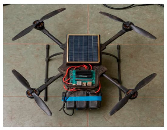
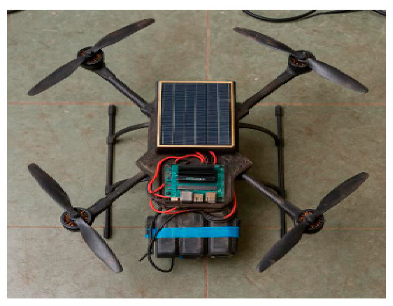
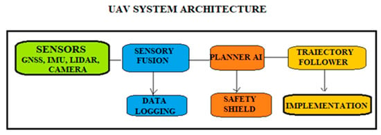
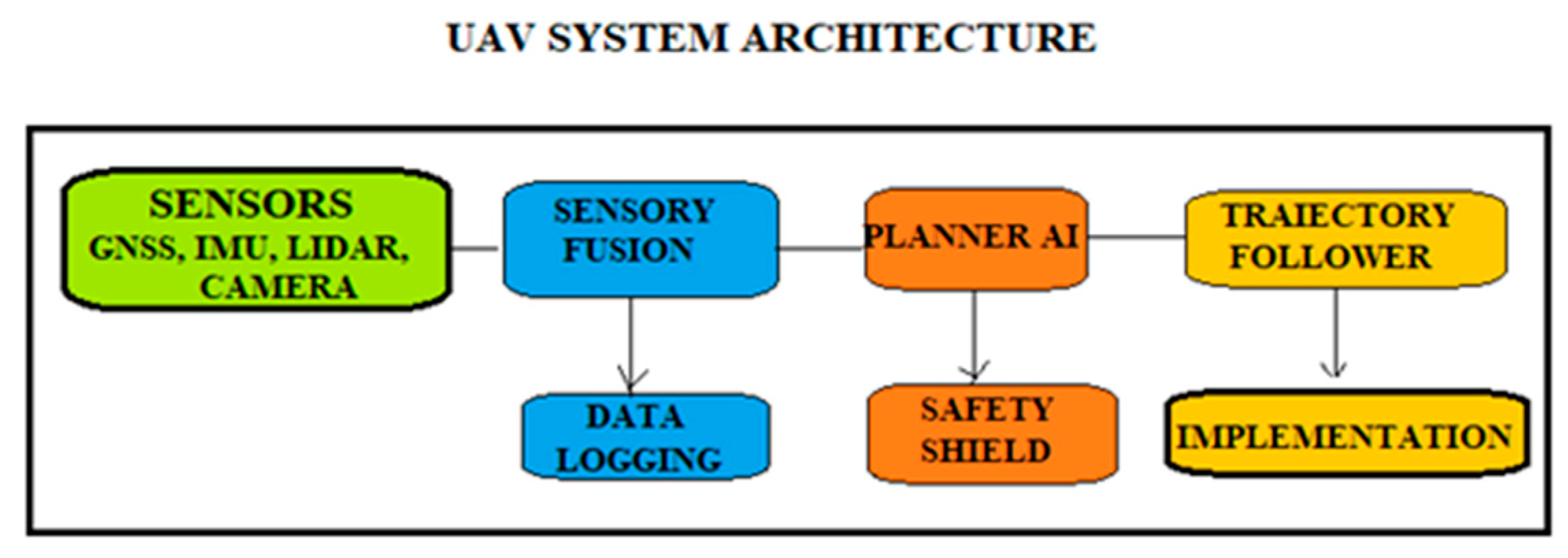
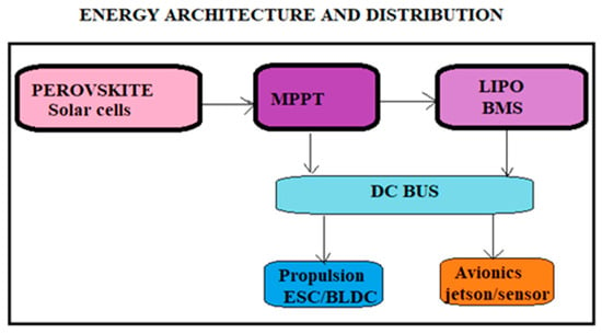
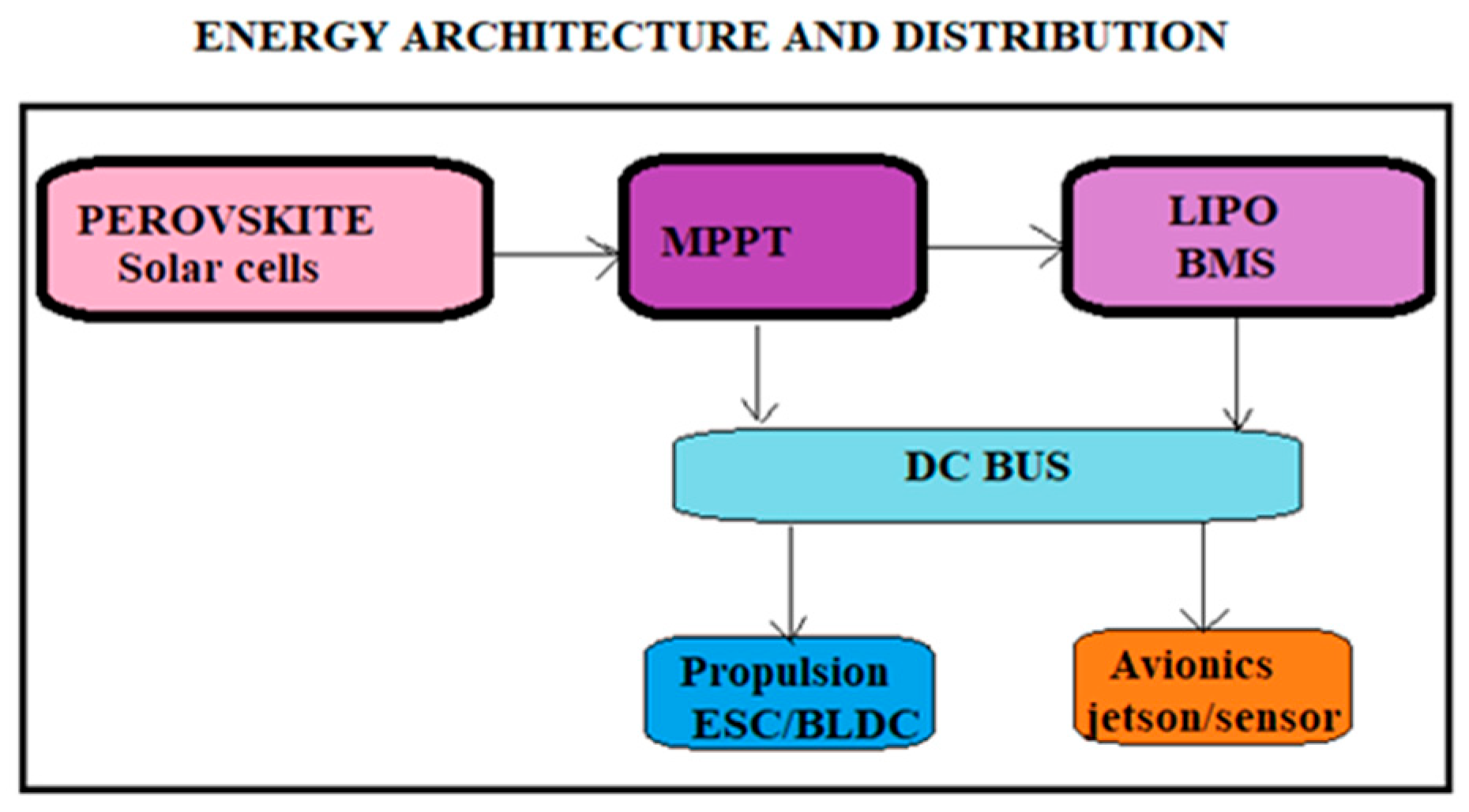
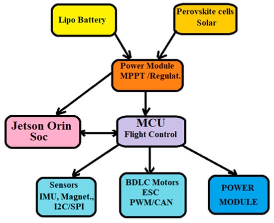
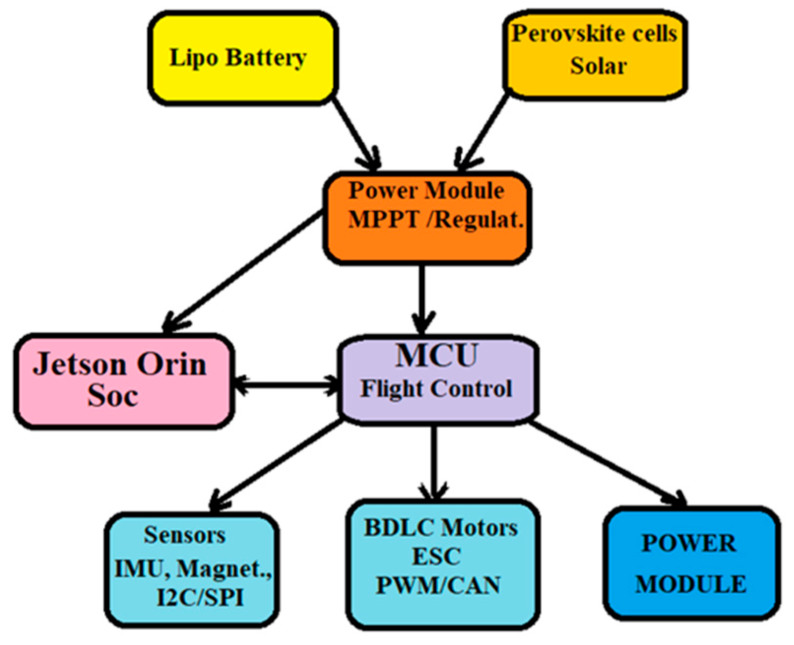
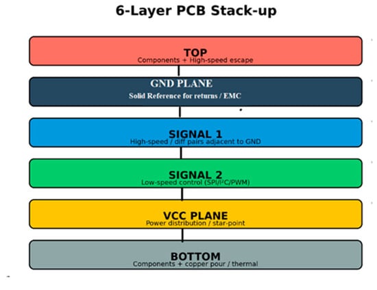
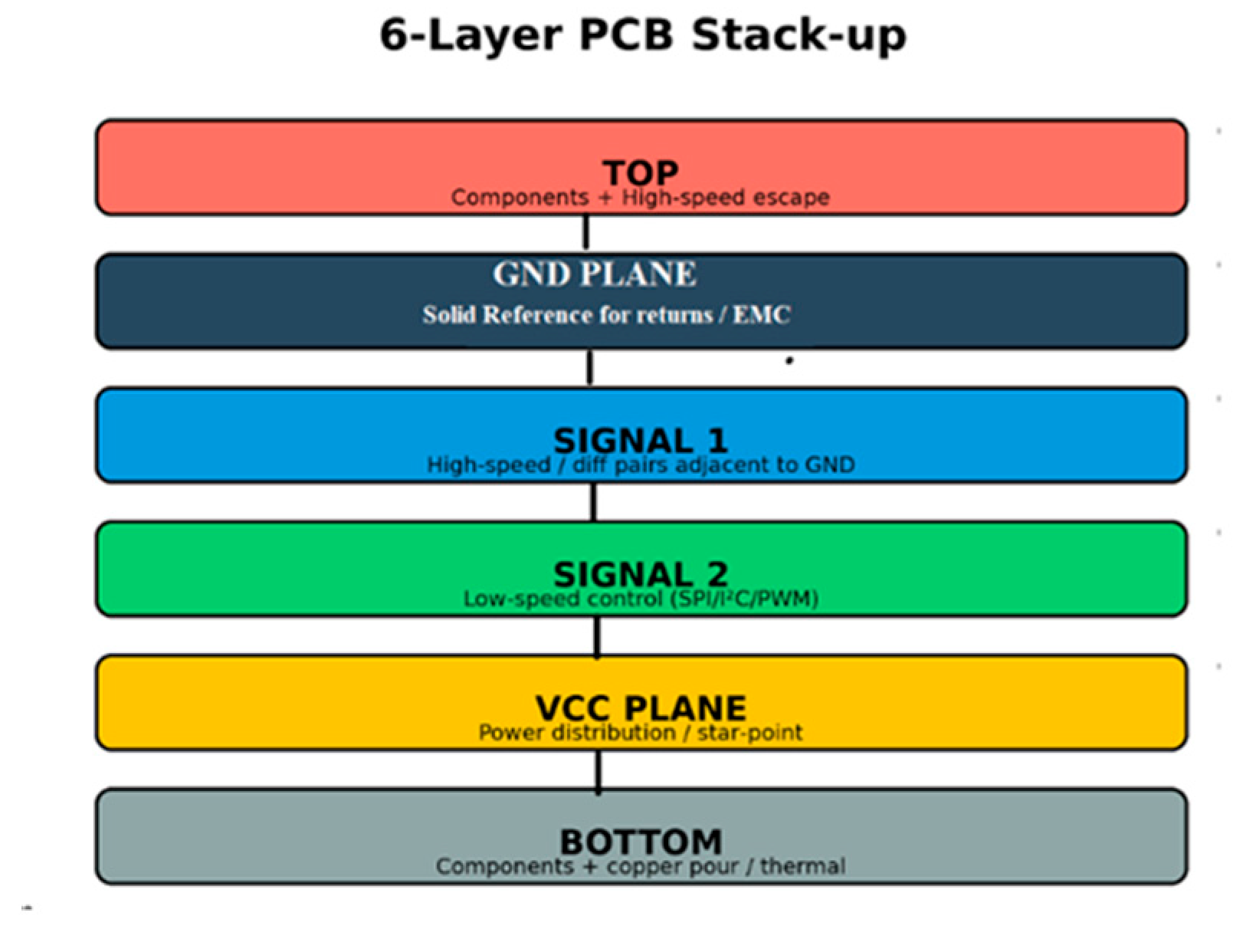
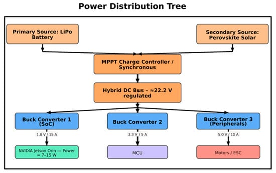
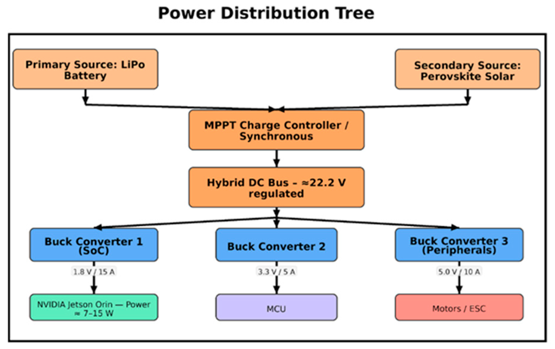
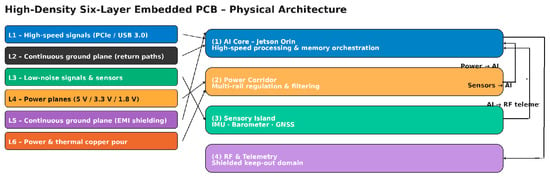
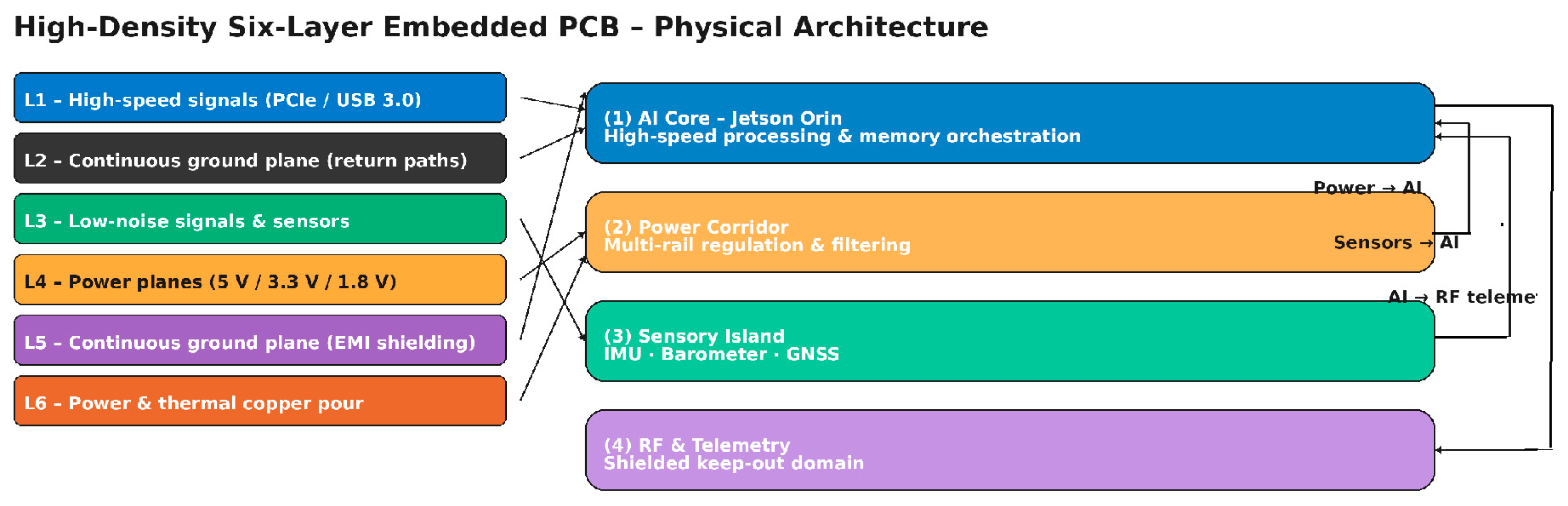
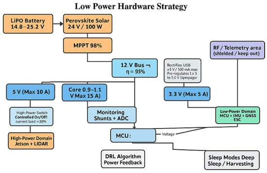
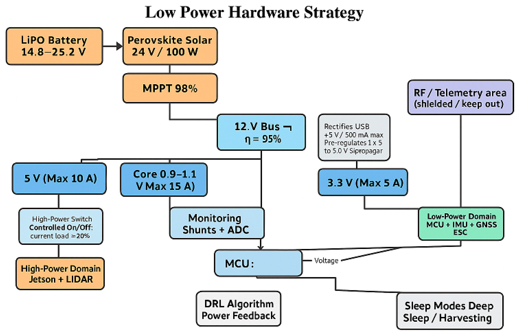
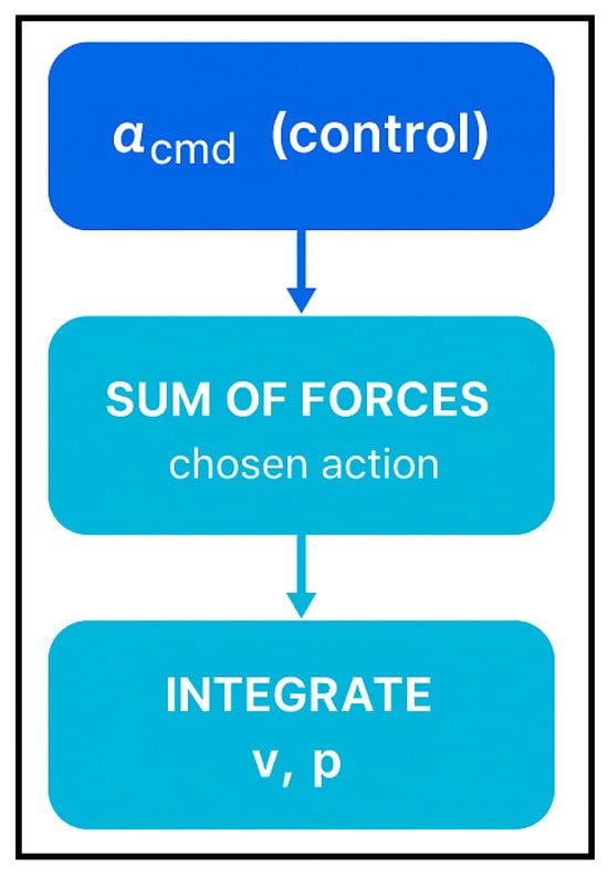
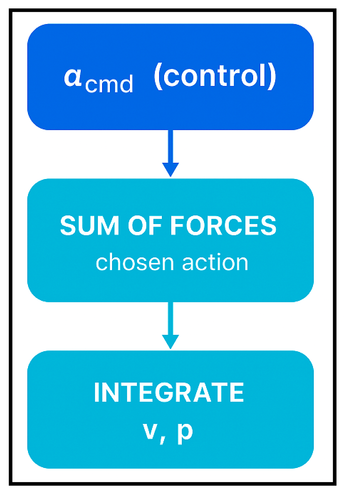
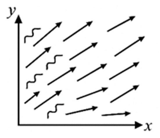
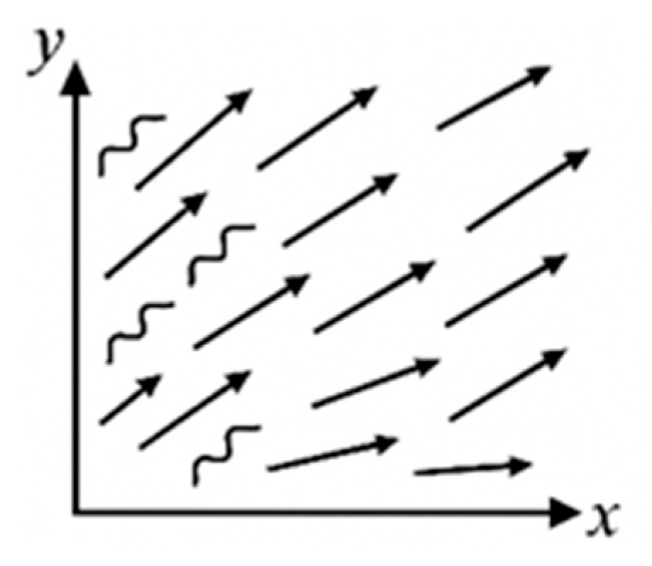
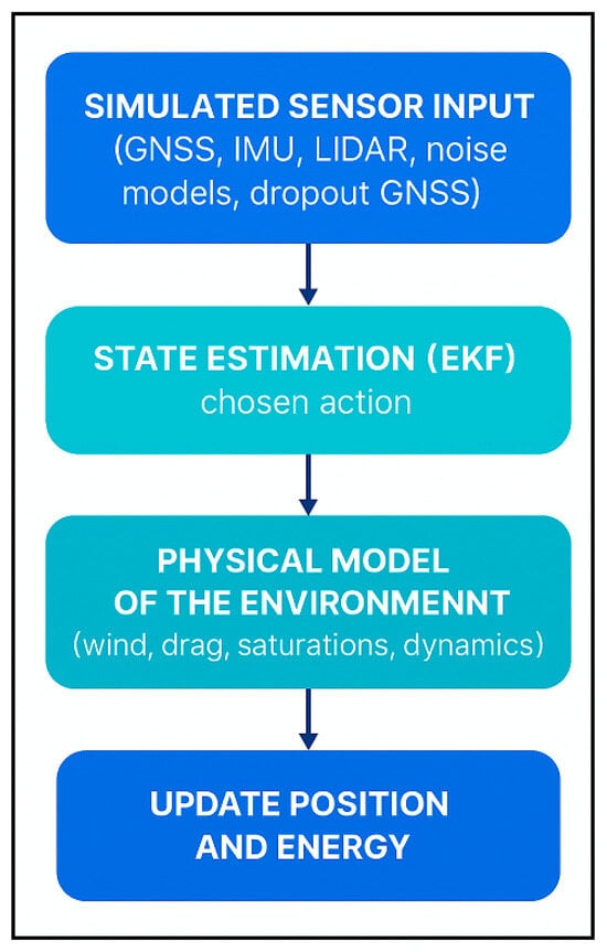
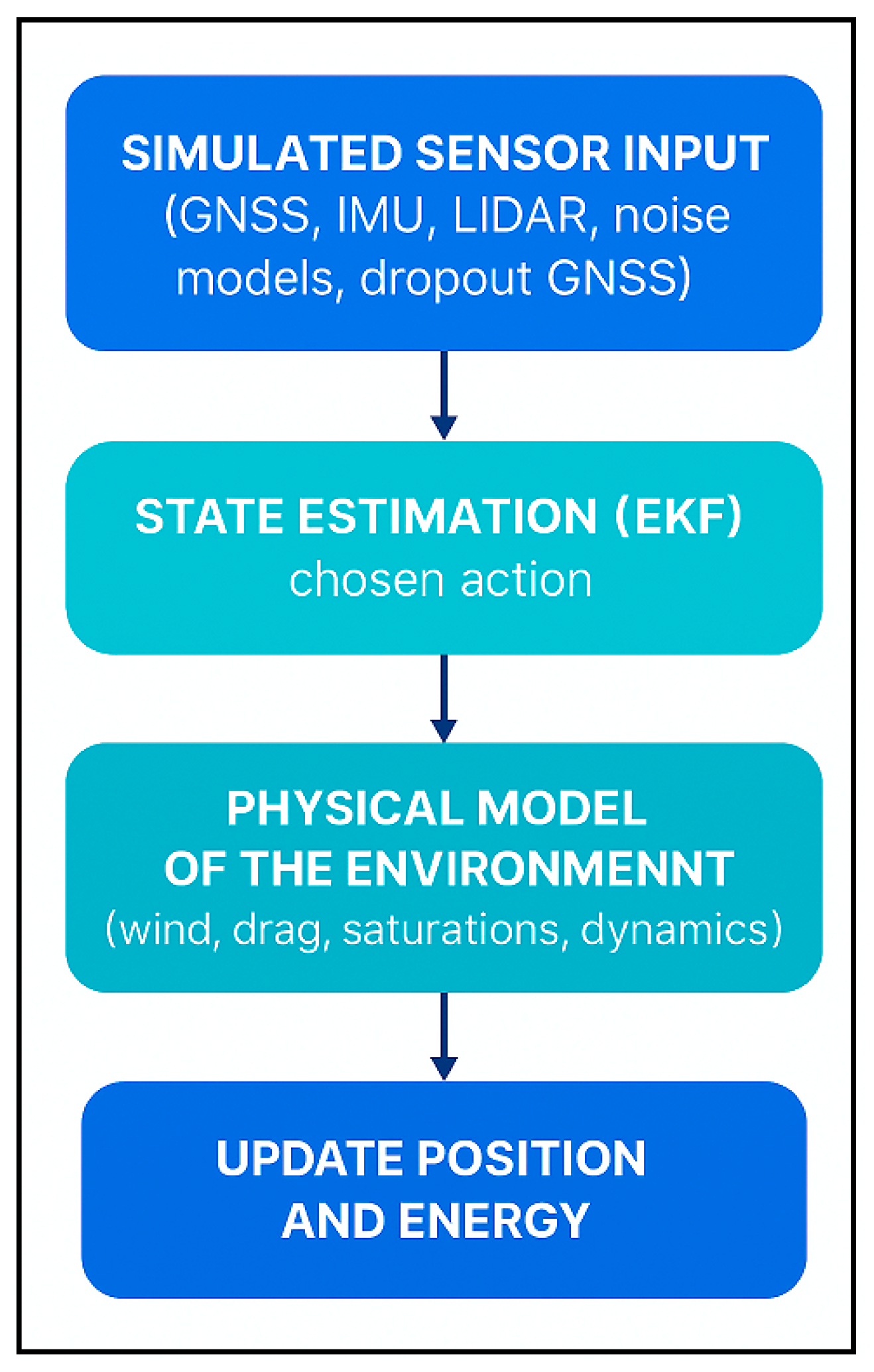
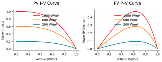
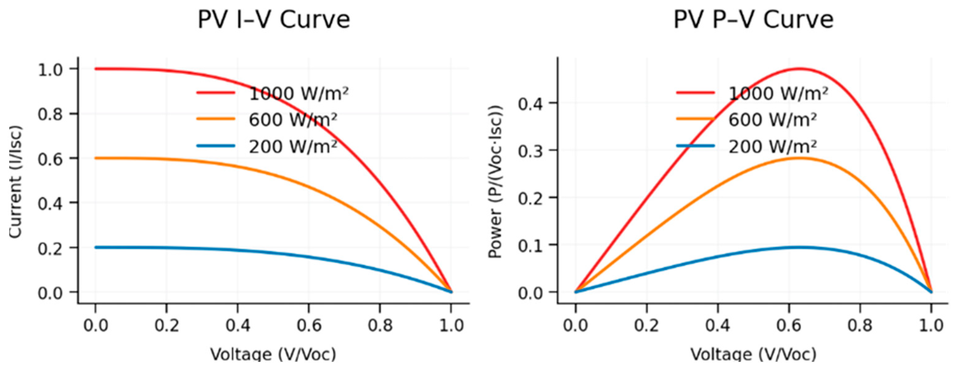
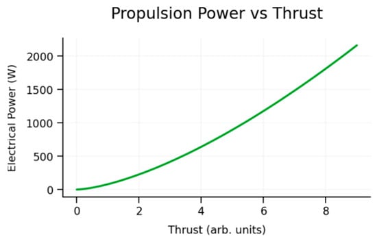
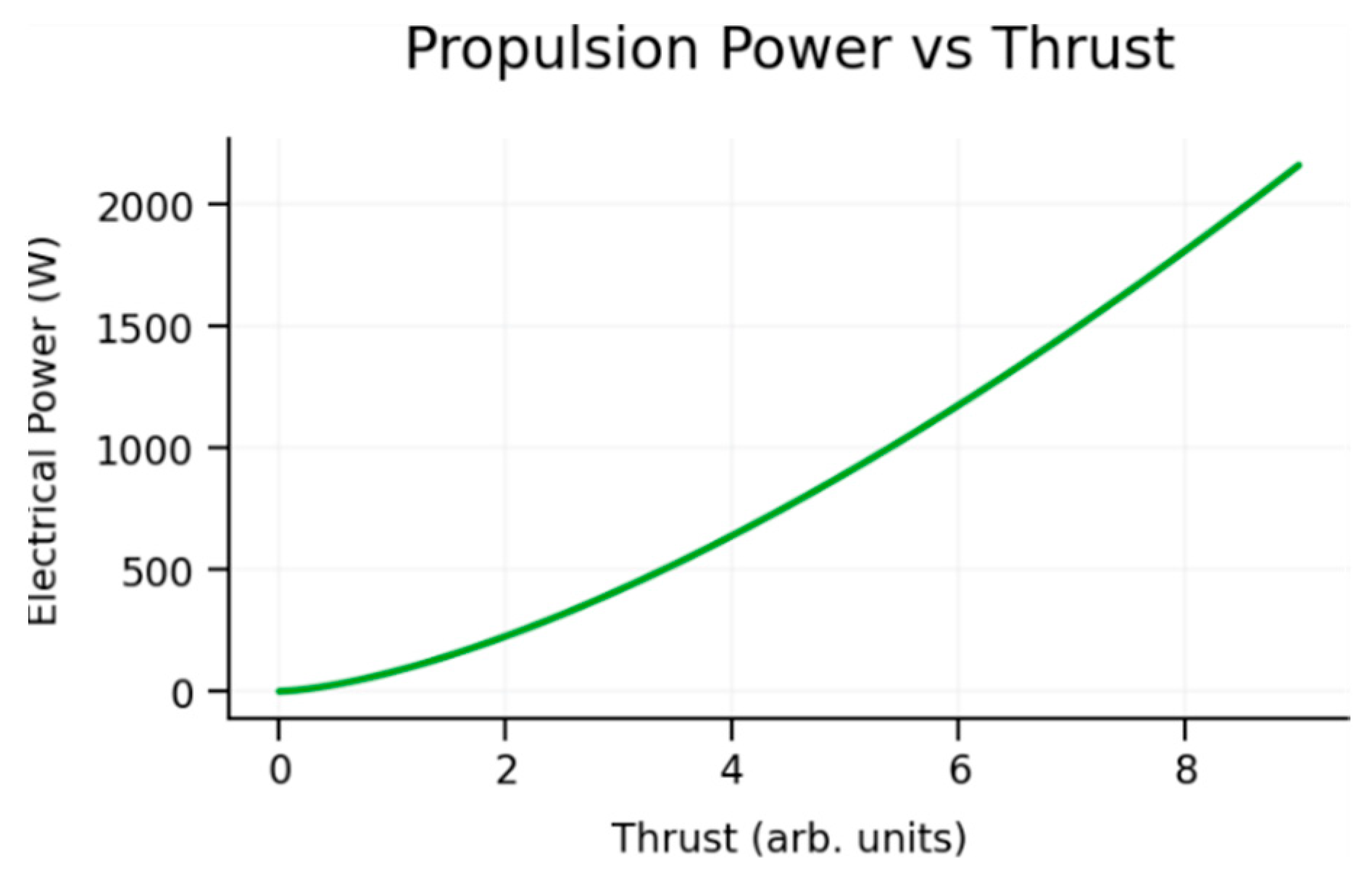
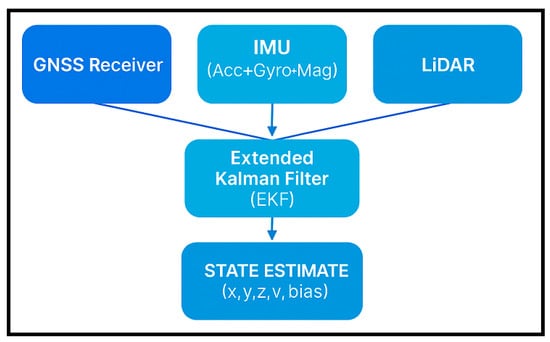
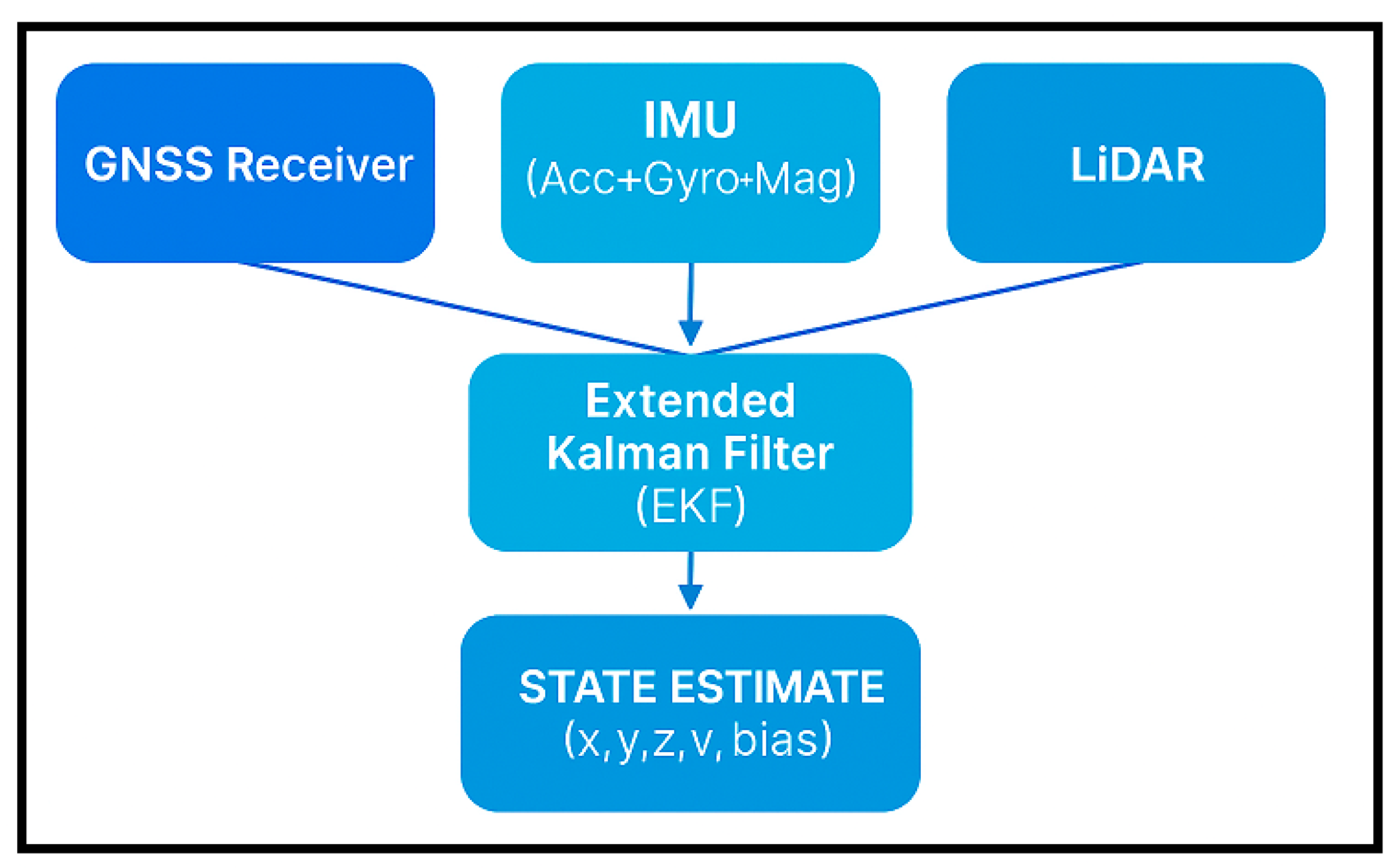
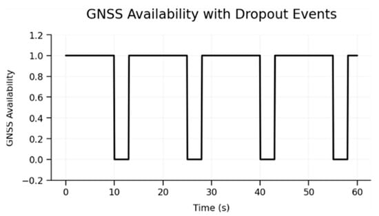
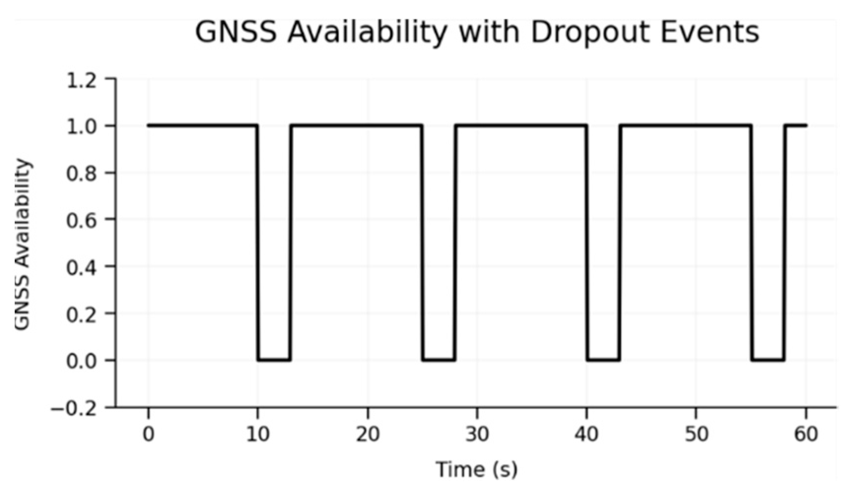
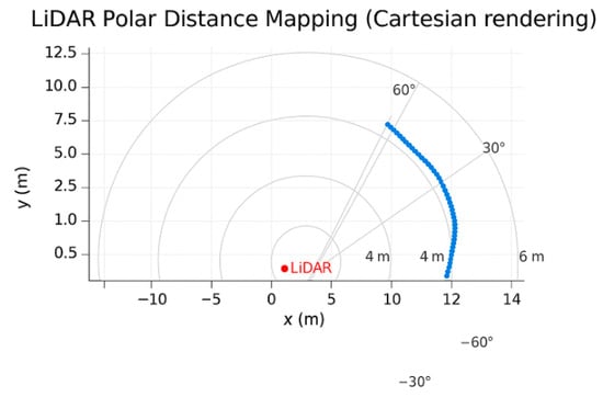
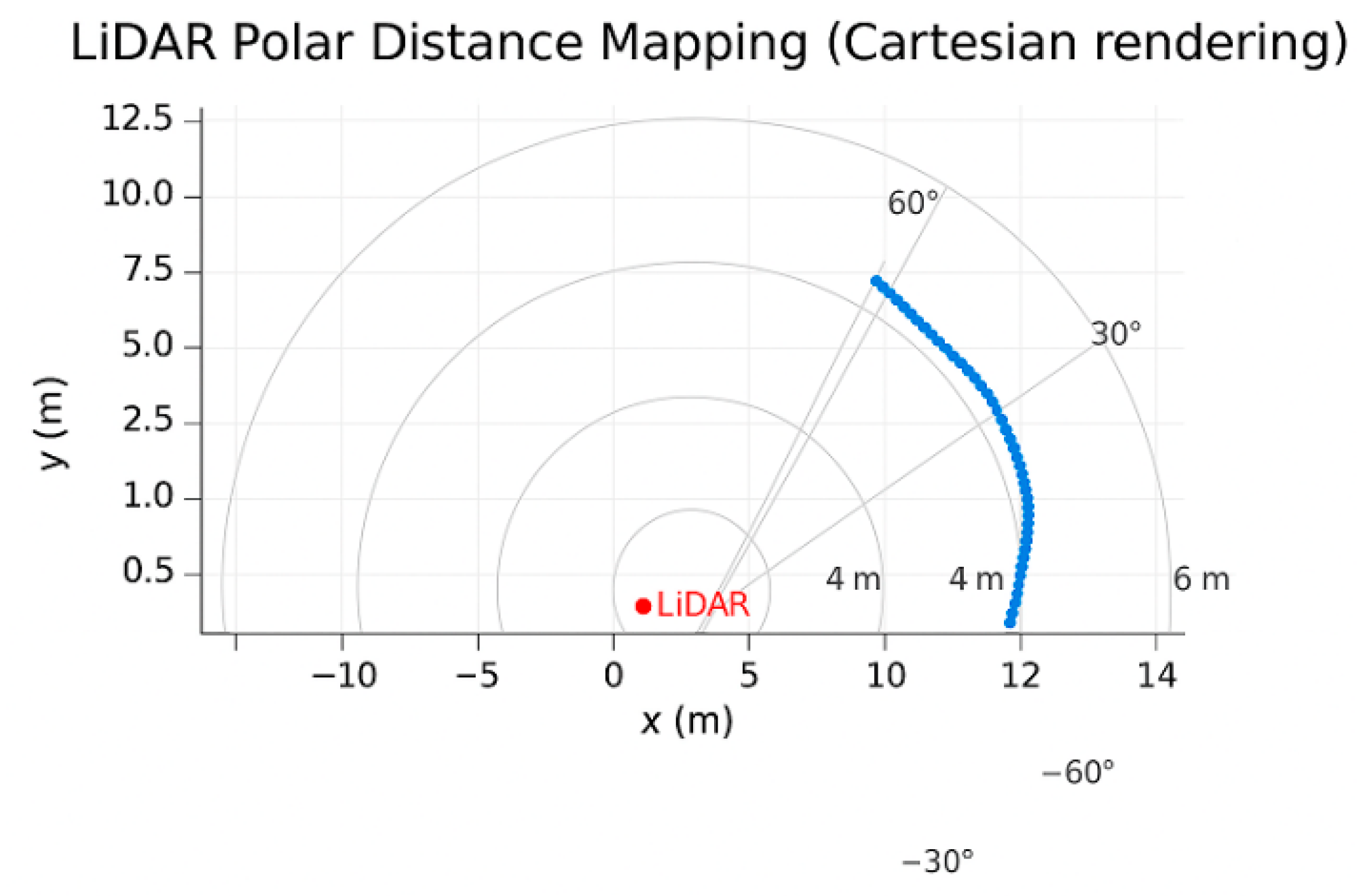
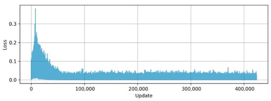
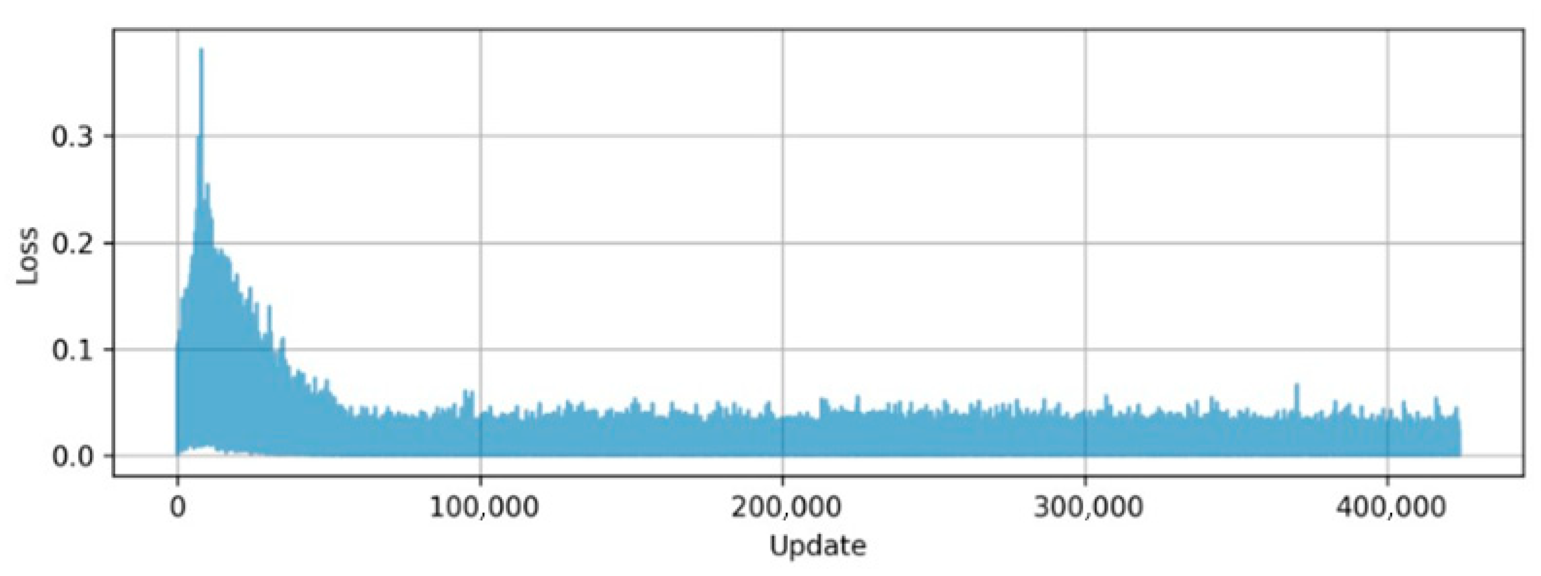
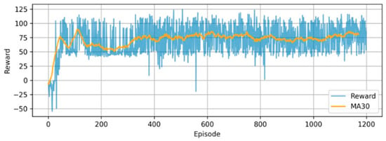
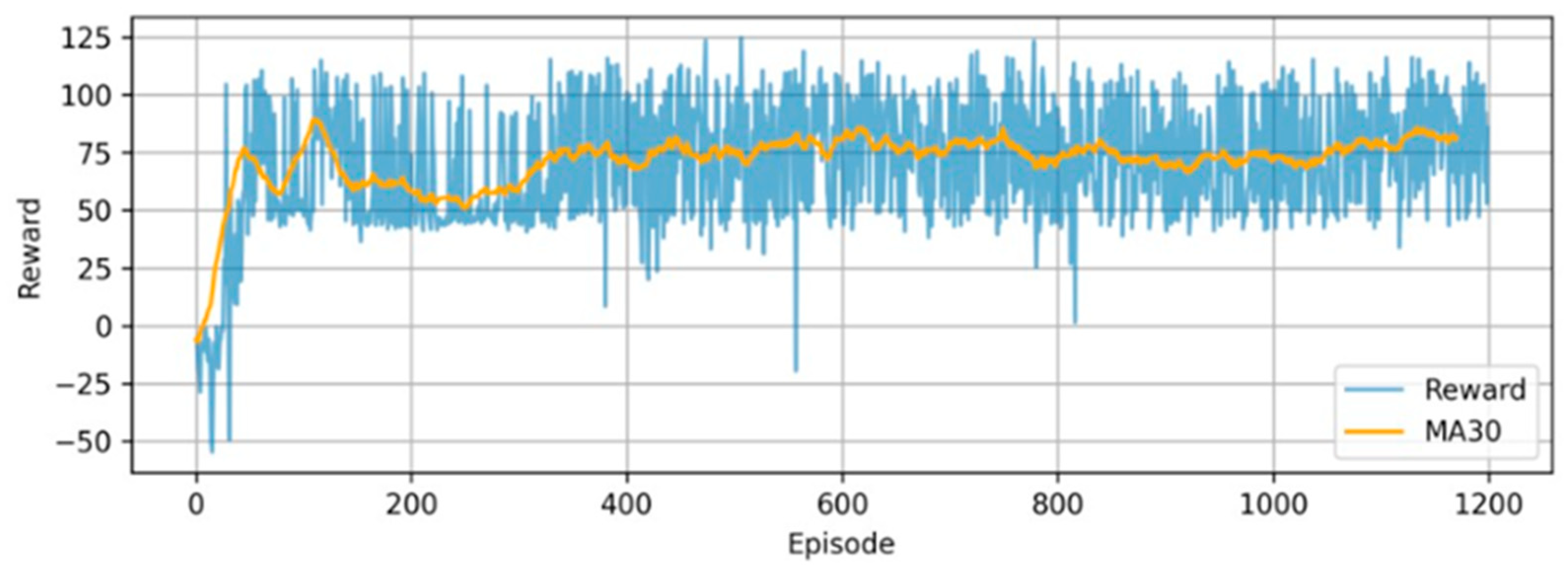
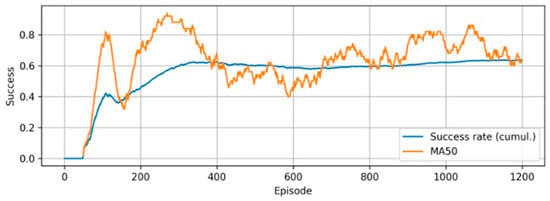
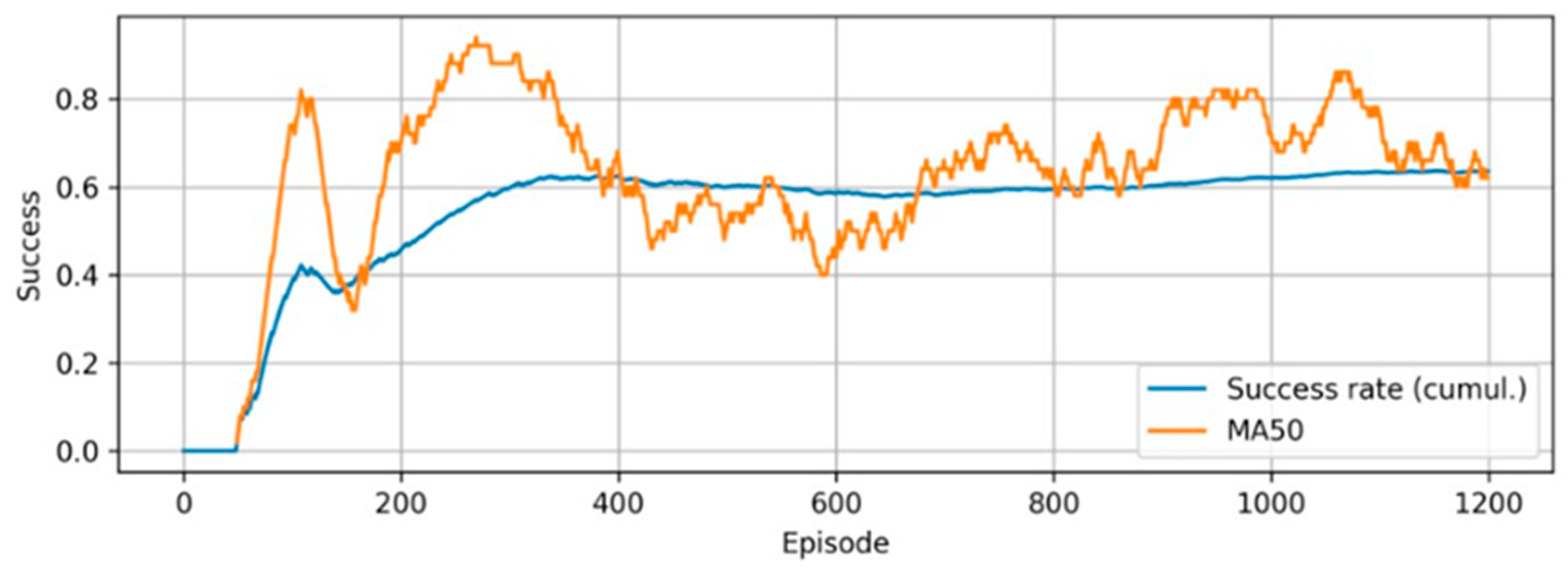
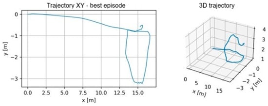
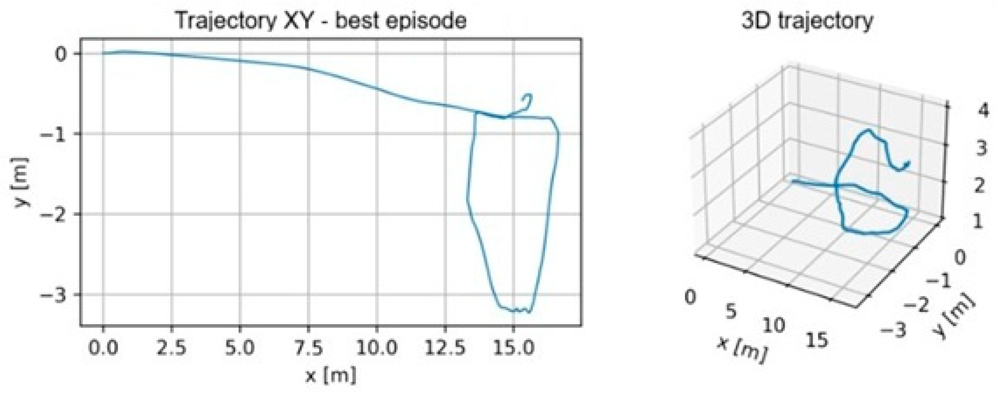
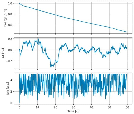
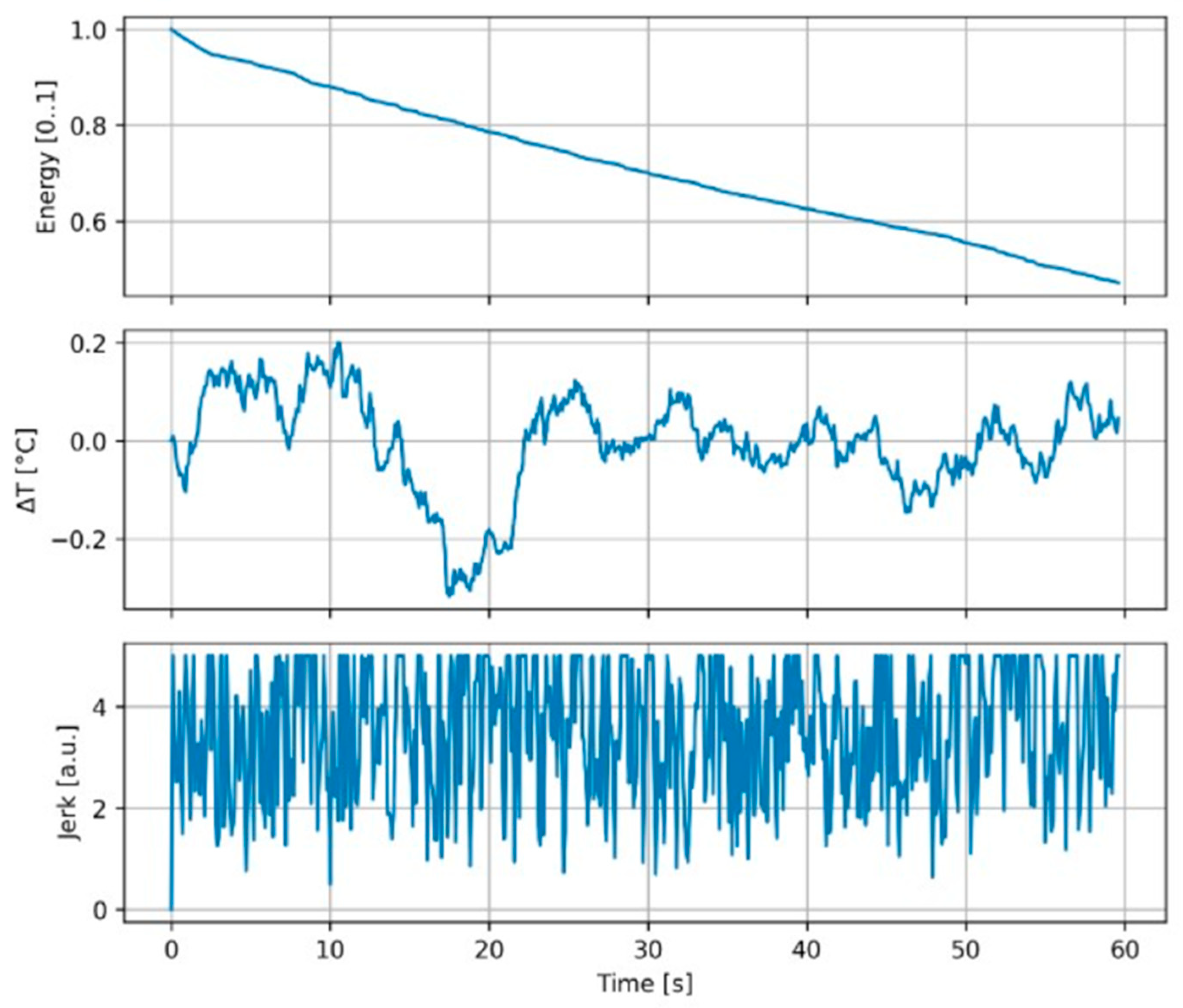
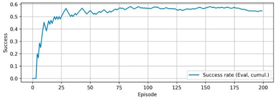
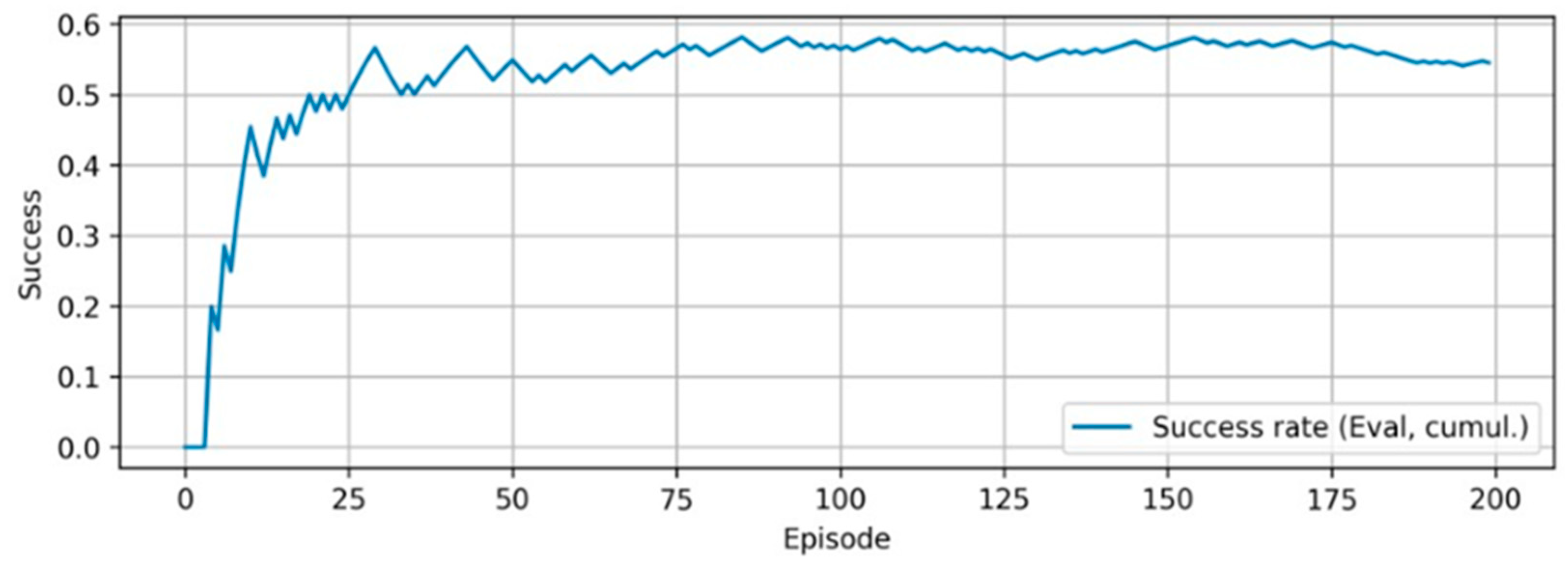
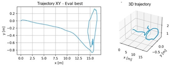
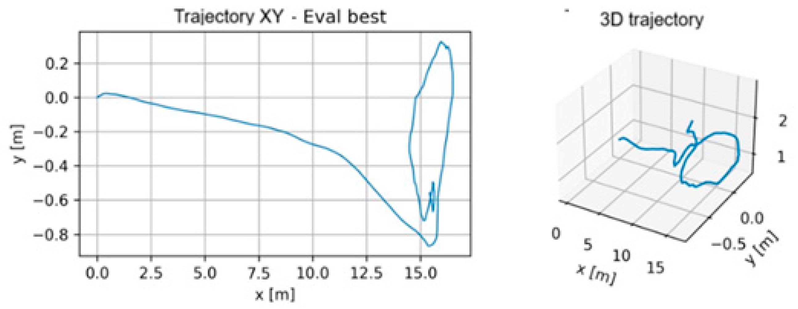
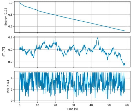
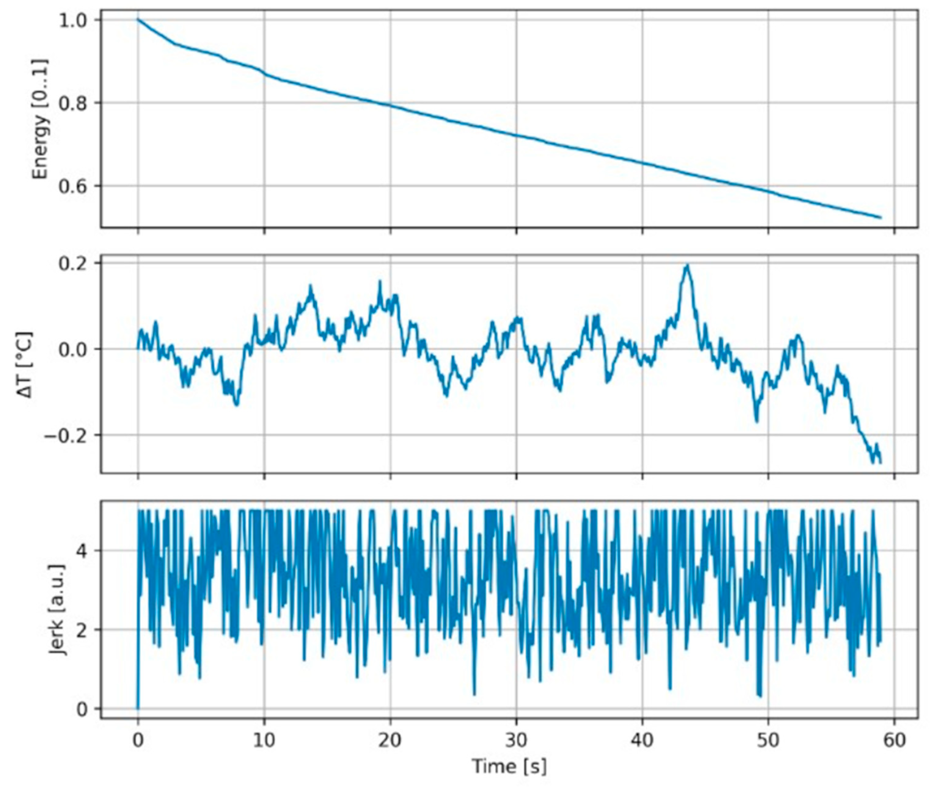

Disclaimer/Publisher’s Note: The statements, opinions and data contained in all publications are solely those of the individual author(s) and contributor(s) and not of MDPI and/or the editor(s). MDPI and/or the editor(s) disclaim responsibility for any injury to people or property resulting from any ideas, methods, instructions or products referred to in the content. |
© 2026 by the authors. Licensee MDPI, Basel, Switzerland. This article is an open access article distributed under the terms and conditions of the Creative Commons Attribution (CC BY) license.