Coordinated Optimization Method for Post-Disaster Transmission Line Repair and System Restoration Against Ice and Snow Disasters

Abstract

A coordinated optimization method for emergency repair scheduling and system operation restoration is proposed to address large-scale transmission line outages caused by extreme weather events such as ice and snow disasters. First, an active outage scenario for transmission lines is constructed based on the Jones icing thickness model and an exponential failure probability model, while incorporating the spatial distribution characteristics of ice disasters. Subsequently, a bi-level optimization model with repair resource constraints is developed. The upper-level model determines the transmission line repair schedule with the objective of minimizing the total repair time while taking system power supply restoration efficiency into account. Based on the completion times of line repairs, the lower-level model optimizes the system restoration process by considering power flow constraints, generator start-up processes, and load restoration characteristics. To address the challenges posed by discrete operational states and strongly coupled bi-level constraints that are difficult to solve using conventional approaches, a logic-based Integer L-shaped coordinated solution method is proposed. Finally, the effectiveness of the proposed method is validated through case studies based on the IEEE New England 10-unit 39-bus system. The results demonstrate that the proposed method can significantly improve system load restoration levels while maintaining high repair efficiency.

1. Introduction

With the expansion of power grid scale, increasing interconnectivity, and growing operational complexity, the impact of ice and snow disasters on the secure operation and post-disaster restoration of transmission systems has become increasingly significant. In early 2008, a severe ice storm struck southern China, causing extensive damage to transmission lines and towers and resulting in substantial economic and social losses [1]. In early 2024, China again experienced widespread rain, snow, and freezing weather, which significantly affected the operation of transmission and distribution facilities in some regions [2], further highlighting the vulnerability of large-scale power systems under extreme icing conditions. In recent years, the concept of power system resilience has gradually been introduced into the field of extreme disaster research, providing a theoretical framework for systematically analyzing the disturbance tolerance and restoration capability of power grids under disaster conditions [3].

Considerable research has been conducted on icing risk identification and transmission line failure mechanisms. Reference [4] systematically reviews the formation mechanisms of transmission line icing and points out that icing can readily lead to conductor breakage, line tripping, and equipment damage. With regard to icing prediction, Reference [5] proposes a support vector machine-based method for forecasting icing loads on overhead transmission lines, while Reference [6] develops a deep learning-based model for predicting ice thickness, further improving prediction accuracy. In terms of de-icing technologies, existing approaches mainly include thermal de-icing (ice melting by high AC/DC current), mechanical de-icing (manual knocking and pulley scraping), and de-icing robots [4,7]. However, these methods have limitations in large-scale ice disaster scenarios, such as restricted coverage and insufficient response capability. When the icing severity exceeds the capacity of online de-icing measures, proactive line outages and post-disaster repair remain necessary means to ensure secure system operation.

Regarding pre-disaster preventive dispatch and operational optimization, Reference [8] proposes a preventive dispatch method considering icing impacts, which mitigates the effects of ice disasters on transmission systems by adjusting generation schedules in advance. In the area of resilience assessment and enhancement, Reference [9] presents methods for evaluating and improving transmission system resilience against ice disasters, while Reference [10] proposes a full-timescale resilience enhancement framework for transmission systems under ice disasters, providing systematic modeling from pre-disaster prevention to post-disaster restoration. Beyond disaster-specific resilience frameworks, recent studies have also explored grid resilience enhancement from complementary perspectives. Reference [11] investigates a power grid optimization operation and resilience improvement strategy considering the participation of energy storage resource aggregation, showing that coordinated scheduling of aggregated flexible resources can effectively enhance grid resilience. Reference [12] further proposes a collaborative optimization model that jointly considers post-disaster damage repair and power system operation for transmission systems, and demonstrates through a mixed-integer second-order cone formulation that coordinating repair activities with system operation can significantly reduce power outage losses. However, these works either focus on normal or moderately stressed operating conditions or consider general fault scenarios without capturing the impact of proactive de-energization on the initial state of post-disaster restoration under extreme ice disasters. Compared with pre-disaster risk identification and resilience enhancement, the post-disaster restoration stage more directly determines outage duration and the level of power supply restoration. Therefore, further attention should be given to the coordinated optimization of repair scheduling and system restoration.

Existing studies on the coordination of post-disaster repair and system restoration have focused mainly on distribution networks. Reference [13] models the post-disaster repair process of distribution networks as a scheduling problem with soft priority constraints and proposes several repair sequence optimization algorithms. Reference [14] investigates the coordinated optimization of repair crew routing and distribution network reconfiguration. Reference [15] proposes a post-disaster restoration strategy for distribution networks that coordinates repair crews, mobile power sources, and network reconfiguration. However, these studies are primarily designed for the radial topology of distribution networks and mostly consider stochastic fault scenarios; research at the transmission network level remains relatively limited.

In summary, existing research on ice disasters has primarily focused on icing prediction, preventive scheduling, and resilience enhancement, with insufficient attention to the coordinated optimization of post-disaster repair scheduling and system operation restoration. Under severe icing conditions, proactive de-energization of heavily iced transmission lines alters the original network topology and causes power flow redistribution, resulting in a strong coupling between repair scheduling and system operation restoration. Current studies remain limited in the following aspects: first, the coordinated optimization of post-disaster repair scheduling and system operation restoration under proactive outage settings has not been thoroughly investigated, making it difficult to adequately capture the impact of proactive de-energization on the initial state and feasible pathways of post-disaster restoration; second, existing coordinated repair-restoration studies are predominantly oriented toward random fault scenarios in distribution networks, with limited modeling efforts directed at proactive outage scenarios in transmission networks, thus failing to effectively characterize the complex coupling among repair resource constraints, network operational constraints, and generator start-up sequences. Moreover, such models involve a large number of discrete operational states and bi-level coupling constraints that are difficult to solve directly using conventional decomposition methods such as Benders decomposition, whereas the logic inference-based Integer L-shaped method [16] provides an effective decomposition framework for this class of bi-level optimization problems with integer variables.

To address the aforementioned issues, this paper proposes a coordinated optimization method for post-disaster transmission line repair and system restoration under ice and snow disaster scenarios. The main contributions of this paper are as follows:

(1)

A proactive outage–line repair–system restoration analytical framework is developed for the scenario of proactive de-energization of heavily iced transmission lines under ice and snow disasters, which clarifies the mechanism through which proactive de-energization affects the initial state and restoration pathways of post-disaster recovery.

(2)

A bi-level optimization model incorporating repair resource constraints is established, in which the upper level determines the line repair scheduling scheme and the lower level optimizes the system restoration process under the corresponding network recovery state, thereby capturing the dynamic coupling between repair scheduling and system operation restoration.

(3)

A logic inference-based Integer L-shaped decomposition method is employed to efficiently solve the proposed bi-level model, overcoming the computational difficulties arising from discrete operational states and bi-level coupling constraints.

2. Ice Disaster Scenario Line Fault Probability and Active Shutdown Scenario Modeling

2.1. Transmission Line Fault Probability Modeling Under Ice Disaster Scenarios

Under extreme ice and snow disasters, the continuous accumulation of ice and snow makes conductor breakage caused by icing the primary cause of transmission line failures [17]. During ice disaster events, transmission lines are mainly subjected to tensile forces induced by wind and ice accretion. Accordingly, the line failure probability model can be established by analyzing the wind load and ice load acting on the line.

In this paper, the icing thickness calculation model proposed by Jones [18] is adopted, and the specific formula is given as follows:

$$D_{\mathrm{ice}}={\displaystyle \frac{t}{\pi {\rho }_{\mathrm{I}}}}\sqrt{{\left(r{\rho }_{\mathrm{W}}\right)}^2+{\left(3.6vW\right)}^2}$$

(1)

where D_ice is the icing thickness in mm; t is the duration of freezing rain in hours; r is the rainfall rate in mm/h; ρ_I and ρ_W are the densities of ice and water, respectively; v is the wind speed in m/s; W is the moisture content in air, taken as 0.067 r^0.864; π is taken as 3.14.

Based on the line icing thickness at time t, the ice load L_I per unit length of line can be obtained from Equation (2):

$$L_I=9.8\times {10}^{-3}{\rho }_1\pi \left(d+D_{\mathrm{ice}}\right)D_{\mathrm{ice}}$$

(2)

where d is the conductor diameter in mm.

Considering the wind speed v_g at the transmission line location at time t, the wind load L_W per unit length of line can be obtained [19] from Equations (3) and (4):

$$L_{\mathrm{W}}=CS{v}^2\left(d+2D_{\mathrm{ice}}\right)$$

(3)

$$S=\left\{\begin{array}{ll}1-(v -2.2352)\times {10}^{-3}\hfill & v >2.2352 \mathrm{m}/\mathrm{s}\hfill \\ 1\hfill & v \le 2.2352 \mathrm{m}/\mathrm{s}\hfill \end{array}\right.$$

(4)

where C is a constant coefficient, valued at 6.964 × 10⁻³; S is the span factor, calculated by Equation (4).

The ice load and wind load can be approximately considered mutually perpendicular, thus the combined ice-wind load L_WI per unit length of transmission line can be obtained from Equation (5):

$$L_{\mathrm{WI}}=\sqrt{L_{\mathrm{I}}^2+L_{\mathrm{W}}^2}$$

(5)

When the line force due to icing exceeds its limit, its fault probability significantly increases. Using the exponential theoretical model proposed in reference [20], the fault probability p_f per unit length of line can be obtained from Equation (6):

$$p_{\mathrm{f}}=\left\{\begin{array}{ll}0\hfill & L_{\mathrm{WI}}\le a_{\mathrm{WI}}\hfill \\ \exp \left({\displaystyle \frac{0.6931(L_{\mathrm{WI}}-a_{\mathrm{WI}})}{b_{\mathrm{WI}}-a_{\mathrm{WI}}}}\right)-1\hfill & a_{\mathrm{WI}}<L_{\mathrm{WI}}<b_{\mathrm{WI}}\hfill \\ 1\hfill & L_{\mathrm{WI}}\ge b_{\mathrm{WI}}\hfill \end{array}\right.$$

(6)

where a_IW and b_IW are the design load and ultimate load of the line for icing bearing capacity, respectively, in N/m.

On this basis, according to the definition of a series system [21], the failure probability $P\left(l\right)$ of a transmission line with length $l$ can be obtained as:

$$P\left(l\right)=1-{\left(1-P_{\mathrm{f}}\right)}^l$$

(7)

Based on the above model, the fault risk level of different transmission lines under ice and snow disaster conditions can be quantitatively assessed, providing a basis for subsequent active shutdown line screening and post-disaster restoration scenario construction.

2.2. Construction of Active Transmission Line Shutdown Scenarios Based on Fault Risk

Since freezing-rain-induced icing can easily lead to flashover and short-circuit faults on insulator surfaces, continued operation of high-risk lines may trigger cascading events such as voltage instability and conductor breakage, thereby further expanding the impact of the disturbance. Therefore, during the disaster evolution stage, proactively disconnecting transmission lines with high failure risk is an effective measure to suppress accident propagation and ensure secure system operation.

To establish transmission line outage scenarios under rain-, snow-, and freezing-related disasters, the coordinates of each node i are first defined as (x_i, y_i), and the distance between nodes is calculated as in (8):

$$d(i,j)=\sqrt{{\left(x_i-x_j\right)}^2+{\left(y_i-y_j\right)}^2}$$

(8)

A disaster center point is established in the coordinate system, and the coordinates of each node are determined according to the standard geographical layout of the IEEE 39-bus system, with units in kilometers. The coordinates of the disaster center point (x_c, y_c) will be specified in the case study. Its location should cover areas where transmission corridors are dense, and generation and load are concentrated, in order to simulate a typical scenario of freezing-rain-type ice disasters radiating outward from the core impact zone. The intensity of the disaster is related to the location of the line and its distance from the disaster center point. The disaster intensity coefficient I_d is defined as in (9):

$$I_d=\max \left(0,1-{\displaystyle \frac{\sqrt{{\left(x-x_c\right)}^2+{\left(y-y_c\right)}^2}}{D_{\max }}}\right)$$

(9)

where the disaster intensity coefficient I_d is a dimensionless value between [0, 1]. I_d = 1 represents the disaster center with the most severe impact; I_d = 0 represents beyond the influence range with no impact; (x_c, y_c) is the disaster center coordinate, while x and y are the coordinates of the line midpoint, used to simplify the line location; D_max is the maximum influence distance of the ice disaster.

I_d is a dimensionless coefficient used to comprehensively characterize the spatial intensity of the disaster. Physically, it represents the ratio of the disaster intensity at a given location to that at the disaster center. Wind speed, rainfall rate, and freezing-rain duration are all linearly scaled by I_d. The rationale is that, under the control of the same frontal weather system, the spatial distributions of these three meteorological variables are all dominated by the overall intensity of the system, and their spatial attenuation trends are generally consistent at the macroscopic scale [1]. This treatment is consistent with the simplified parameterization methods commonly adopted in existing ice-disaster scenario modeling studies [9], and can effectively support scenario construction and transmission line risk screening with reasonable data requirements.

Accordingly, in (1), the wind speed, rainfall rate, and freezing-rain duration are expressed as v = V_base × I_d, r = R_base × I_d, and t_r = T_base × I_d, respectively.

It should be noted that the above linear scaling is an engineering approximation intended to reflect, in a concise parameterized form, the relative variation trends of meteorological factors with the spatial attenuation of disaster intensity, rather than to precisely reproduce the absolute values of each meteorological variable. Accordingly, the unified disaster intensity coefficient I_d proposed in this paper is primarily intended to support scenario construction and post-disaster restoration decision-making, rather than to serve as a high-fidelity meteorological reproduction tool.

Based on the above formulation, the length of each transmission line can be determined, and the failure probability of each transmission line can then be calculated. After screening, the set of lines to be proactively disconnected, denoted by E_f, is finally obtained.

3. Bi-Level Restoration Optimization Model and Solution Method

Under the aforementioned active shutdown scenario, the system restoration process involves both line repair scheduling decisions and system operational state optimization. On one hand, the repair sequence and crew allocation determine the restoration time of outage lines. On the other hand, different line restoration sequences dynamically change system topology structure, thereby affecting power flow distribution, generator start-up processes, and load restoration levels. These two decision processes are mutually coupled and interactive, making them difficult to characterize through a single optimization model.

Bi-level optimization has been widely applied in power system decision-making problems involving hierarchical coupling. For instance, bi-level frameworks have been developed for coordinated power system restoration supported by multiple flexible resources [22], for generator start-up sequencing against cyber attacks [23], and for collaborative planning of multi-energy networks based on double-layer game theory [24]. These studies demonstrate that bi-level formulations are effective in handling coupled decisions across different entities or time scales. However, existing works primarily focus on steady-state operational coordination, planning, or restoration under generic fault scenarios, whereas the problem addressed in this paper involves a distinct coupling between discrete repair scheduling and dynamic system restoration under proactive de-energization induced by ice-disaster conditions.

Therefore, this paper adopts bi-level optimization modeling to hierarchically describe repair scheduling decisions and system operation restoration processes. The upper-level model is responsible for repair scheduling and timing arrangements, while the lower-level model optimizes system operational states under given repair results. Finally, the Integer L-shaped method based on logical inference is used to solve the model, achieving coordinated decision-making for the post-disaster restoration process.

3.1. Upper-Level Model

Suppose w outage lines are determined, with q crews participating in repairs. Each line corresponds to a repair completion time, t_k = t₁, t₂, … t_w; outage line set E_f; repair crew set Q. The time t^recover_ij required to repair each line is determined based on the icing thickness D_ice and length of the transmission line.

Considering computational simplicity, the calculation of crew travel time considers the line midpoint as the starting point. The travel time required for a repair crew to depart from node u to line (i,j) is given by Equation (10), and the travel time from line (k,l) to line (i,j) is given by Equation (11):

$$t_{u,ij}^{\mathrm{route}}={\displaystyle \frac{1}{v_r}}\sqrt{{\left(x_u-{\displaystyle \frac{x_i+x_j}{2}}\right)}^2+{\left(y_u-{\displaystyle \frac{y_i+y_j}{2}}\right)}^2}$$

(10)

$$t_{ij,ol}^{\mathrm{route}}={\displaystyle \frac{1}{v_r}}\sqrt{{\left({\displaystyle \frac{x_i+x_j}{2}}-{\displaystyle \frac{x_o+x_l}{2}}\right)}^2+{\left({\displaystyle \frac{y_i+y_j}{2}}-{\displaystyle \frac{y_o+y_l}{2}}\right)}^2}$$

(11)

where v_r is the movement speed of the repair crew, a fixed constant value. The start time S_ij of line (i,j)repair is given by Equation (12), and the completion time C_ij is given by Equation (13):

$$S_{ij}=\left\{\begin{array}{ll}{t}_{u,ij}^{\mathrm{route}}& ,\mathrm{line} \left(i, j\right) \mathrm{is} \mathrm{the} \mathrm{first} \mathrm{line} \mathrm{repaired} \mathrm{by} \mathrm{team} \mathrm{a}\\ C_{ol}+t_{ol,ij}^{\mathrm{route}}\hfill & ,\mathrm{line} \left(i, j\right) \mathrm{is} \mathrm{not} \mathrm{the} \mathrm{first} \mathrm{line} \mathrm{repaired} \mathrm{by} \mathrm{team} \mathrm{a}\end{array}\right.$$

(12)

$$C_{ij}=S_{ij}+t_{ij}^{\mathrm{recover}}$$

(13)

When all outage lines are repaired, the time T when the last line is repaired is the total repair time, given by Equation (14):

$$t_w=T=\max C_{ij}$$

(14)

The upper-level model objective function is given by Equation (15):

$$\min T-\lambda \eta$$

(15)

where η represents the upper-level decision variable indicating system power supply restoration efficiency, whose actual value is constrained by lower-level optimization results; λ is a weighting coefficient; T is the total repair time.

To satisfy the linear structure requirements of the Integer L-shaped method, the nonlinear total repair time expression T and constraints need to be linearized. The linearized constraint conditions are given by Equations (16)–(22):

$${\displaystyle \sum _{a\in Q}{x}_{ij,a}}=1,\hspace{1em}\forall (i,j)\in E_f$$

(16)

$$C_{ij}=S_{ij}+t_{ij}^{\mathrm{recover}}, \forall (i,j)\in E_f$$

(17)

$$S_{ij}\ge t_{u,ij}^{\mathrm{route}},\hspace{1em}\forall (i,j)\in E_f$$

(18)

$$S_{ij}\ge C_{ol}+t_{ol,ij}^{\mathrm{route}}-M(1-y_{ij,ol})-M(2-x_{ij,a}-x_{ol,a})$$

(19)

$$S_{ol}\ge C_{ij}+t_{ij,ol}^{\mathrm{route}}-M\cdot y_{ij,ol}-M(2-x_{ij,a}-x_{ol,a})$$

(20)

$$T\ge C_{ij},\forall (i,j)\in E_f$$

(21)

$$S_{ij},C_{ij},T\ge 0$$

(22)

$${\displaystyle \sum _{(o,l)\in E_f,(o,l)\ne (i,j)}{y}_{ol,ij}}\le 1,\hspace{1em}\forall (i,j)\in E_f$$

(23)

$${\displaystyle \sum _{(k,h)\in E_f,(k,h)\ne (i,j)}{y}_{ij,kh}}\le 1,\hspace{1em}\forall (i,j)\in E_f$$

(24)

$$U_{ij}\ge U_{ol}+1-M\left(1-y_{ol,ij}\right),\hspace{1em}\forall (o,l)\ne (i,j)\in E_f$$

(25)

$$1\le U_{ij}\le \left|E_f\right|,\hspace{1em}\forall (i,j)\in E_f$$

(26)

where x_ij,a equals 1 if line (i,j) is repaired by crew a, otherwise 0; y_ol,ij equals 1 if line (i,j) is repaired immediately after line (o,l), otherwise 0; U_ij denotes the access order of line (i,j) in the task sequence of its assigned repair team; M is a sufficiently large constant.

Equation (16) indicates that each line is restored by only one crew; Equation (17) represents the completion time of line (i,j) repair; Equation (18) represents the lower bound of the start time for line (i,j) repair; Equations (19) and (20) indicate that a crew can only repair one line at a time. Equations (23) and (24) specify that each repair task has at most one direct predecessor and one direct successor. Equations (25) and (26) impose the sequence order of repair tasks and eliminate subtours.

The repair time for each line is jointly determined by base repair time, line length factor, and ice disaster intensity factor, calculated by Equation (27):

$$t_{ij}^{\mathrm{recover}}=t_{base}+\alpha L+\beta I_d$$

(27)

where t_base is the base repair time; α is the length factor; L is the line length; β is the intensity factor; I_d is the disaster intensity coefficient at the line location.

3.2. Lower-Level Model

Given the repair completion time sequence, the lower-level model aims to maximize system load restoration efficiency. The objective function is given by Equation (28):

$$\max {\displaystyle \frac{{\displaystyle \sum _{k=1}^w{\displaystyle \sum _{i=1}^N{P}_{t_k,i}}}(t_k-t_{k-1})}{T}}$$

(28)

where N is the number of load nodes; w is the number of time periods; $P_{t_k,i}$ is the load at node i at time t_k.

Constraints include:

(1)

Power Flow Constraints

Adopt a linearized AC power flow model

$$P_{t_k,i}=P_{t_k}^{\mathrm{g}}-P_{t_k}^S\left(1-u_{t_k}^S\right)+{\displaystyle \sum _{j:(ji)\in E}{P}_{ji,t_k}}-{\displaystyle \sum _{j:(ij)\in E}{P}_{ij,t_k}},\hspace{1em}g\in G(i)$$

(29)

$$\begin{array}{l}{P}_{t_k,i}\tan {\phi }_i=Q_{t_k}^{\mathrm{g}}-{\displaystyle \sum _{j:(ij)\in E}{Q}_{ij,t_k}}+{\displaystyle \frac{1}{2}}{\displaystyle \sum _{j:(ji)\in E}{B}_{ji,t_k}}{u}_{ji,t_k}+{\displaystyle \frac{1}{2}}{\displaystyle \sum _{j:(ij)\in E}{B}_{ij,t_k}}{u}_{ij,t_k}\\ i=1,2,\cdots ,N,t_k=t_1,t_2,\cdots t_w,g\in G(i)\end{array}$$

(30)

$$-M\left(1-u_{ij,t_k}\right)⩽P_{ij,t_k}-B_{ij}\left({\theta }_{i,t_k}-{\theta }_{j,t_k}\right)+G_{ij}\left(V_{i,t_k}-V_{j,t_k}\right)⩽M\left(1-u_{ij,t_k}\right),\hspace{1em}ij\in E$$

(31)

$$-M\left(1-u_{ij,t_k}\right)⩽Q_{ij,t_k}-G_{ij}\left({\theta }_{i,t_k}-{\theta }_{j,t_k}\right)+B_{ij}\left(V_{i,t_k}-V_{j,t_k}\right)⩽M\left(1-u_{ij,t_k}\right),\hspace{1em}ij\in E$$

(32)

where $P_{t_k}^g$ is the active power output of the generating unit in period $t_k$; $P_{t_k}^S$ is the power required for unit startup in period $t_k$; $u_{t_k}^S$ is a state variable indicating whether the faulty generating unit is in the restart state in period $t_k$, which takes the value of 1 if in the restart state and 0 otherwise; $P_{ji,t_k}$ is the active power flowing through line ji in the transmission network in period $t_k$; E is the set of lines in the transmission network; G(i) is the set of generating units directly connected to node i; $Q_{t_k}^g$ is the reactive power output of the generating unit in period $t_k$; $Q_{ji,t_k}$ is the reactive power flowing through line ji in period $t_k$; $u_{ij,t_k}$ is a state variable representing the operation state of line ij in period $t_k$, which takes the value of 1 if the line operates normally and 0 otherwise; $B_{ji,t_k}$ is the shunt susceptance of line ij; ${\phi }_i$ is the power factor of node i; B_ij and G_ij are the mutual susceptance and mutual conductance between node i and node j, respectively; ${\theta }_{i,t_k}$ and $V_{i,t_k}$ are the voltage phase angle and voltage magnitude of node i in period $t_k$, respectively; M is a sufficiently large constant.

(2)

Generating Unit Constraints

$$P_{t_k,m}^{\mathrm{g},\min }⩽P_{t_k,m}^{\mathrm{g}}⩽P_{t_k,m}^{\mathrm{g},\max }$$

(33)

$$Q_{t_k,m}^{\mathrm{g},\min }⩽Q_{t_k,m}^{\mathrm{g}}⩽Q_{t_k,m}^{\mathrm{g},\max }$$

(34)

$$\left|P_{t_{k+1},m}^{\mathrm{g}}-P_{t_k,m}^{\mathrm{g}}\right|⩽K_{p,m}(t_{k+1}-t_k)$$

(35)

$$\left|Q_{t_{k+1},m}^{\mathrm{g}}-Q_{t_k,m}^{\mathrm{g}}\right|⩽K_{p,m}(t_{k+1}-t_k)$$

(36)

where $P_{t_k,m}^{\mathrm{g},\max }$ and $P_{t_k,m}^{\mathrm{g},\min }$ are the upper and lower limits of the active power output of the m-th generating unit in period $t_k$, respectively; $Q_{t_k,m}^{\mathrm{g},\max }$ and $Q_{t_k,m}^{\mathrm{g},\min }$ are the upper and lower limits of the reactive power output of the m-th generating unit in period $t_k$, respectively; $K_{p,m}$ is the ramp rate of generating unit m.

(3)

Linearized Startup Constraints of Generating Units

$$P_{m,t_k}=x_{1m,t_k}\left\{K_{p,m}(t_k-T_{si,m}-T_{si1,m})\right\}+x_{2m,t_k}\left\{P_{GN,m}-K_{p,m}(t_k-T_{si,m}-T_{si1,m})\right\}$$

(37)

$$x_{1m,t_k}⩾\left(t_k-T_{si,m}-T_{si1,m}\right)/M+1/M^2$$

(38)

$$x_{1m,t_k}⩽1+\left(t_k-T_{si,m}-T_{si1,m}\right)/M$$

(39)

$$x_{2m,t_k}⩾\left(t_k-T_{si,m}-T_{si1,m}-T_{si2,m}\right)/M+1/M^2$$

(40)

$$x_{2m,t_k}\le 1+\left(t_k-T_{si,m}-T_{si1,m}-T_{si2,m}\right)/M$$

(41)

$$D_{m,t_k}⩾\left(t_k-T_{si,m}\right)/M+1/M^2$$

(42)

$$D_{m,t_k}⩽1+\left(t_k-T_{si,m}\right)/M$$

(43)

$$C_{m,t_k}⩾\left(t_k-T_{si,m}-T_{si1,m}\right)/M+1/M^2$$

(44)

$$C_{m,t_k}⩽1+\left(t_k-T_{si,m}-T_{si1,m}\right)/M$$

(45)

where $T_{si,m}$ is the startup time of generating unit m; $T_{si1,m}$ is the ramp preparation time of generating unit m; $T_{si2,m}$ is the ramp duration time of generating unit m; $P_{m,t_k}$ is the active power output of generating unit m in period $t_k$; $P_{GN,m}$ is the rated active power of generating unit m; $D_{m,t_k}$ represents the startup state of generating unit m in period $t_k$; $C_{m,t_k}$ represents the grid-connected state of generating unit m in period $t_k$; $x_{1m,t_k}$ and $x_{2m,t_k}$ denote the intermediate variables of the piecewise function; M is a sufficiently large positive constant.

(4)

Load Node Constraints

$$P_{t_k,i}^{\min }⩽P_{t_k,i}⩽P_{t_k,i}^{\max }$$

(46)

$$Q_{t_k,i}^{\min }⩽Q_{t_k,i}⩽Q_{t_k,i}^{\max }$$

(47)

$$V^{\min }⩽V_{i,t_k}⩽V^{\max }$$

(48)

where $P_{t_k,i}^{\max }$ and $P_{t_k,i}^{\min }$ are the maximum and minimum values of $P_{t_k,i}$, respectively; $Q_{t_k,i}$ is the reactive power at node i of the transmission network in period $t_k$ during the restoration process; $Q_{t_k,i}^{\max }$ and $Q_{t_k,i}^{\min }$ are the maximum and minimum values of $Q_{t_k,i}$, respectively; $V^{\min }$ and $V^{\max }$ are the minimum and maximum values of the node voltage, respectively.

(5)

Line Operation Constraints

$$u_{ij,t_k}{P}_{ij,t_k}^{\min }⩽P_{ij,t_k}⩽u_{ij,t_k}{P}_{ij,t_k}^{\max }$$

(49)

$$u_{ij,t_k}{Q}_{ij,t_k}^{\min }⩽Q_{ij,t_k}⩽u_{ij,t_k}{Q}_{ij,t_k}^{\max }$$

(50)

$${\theta }^{\min }⩽{\theta }_{i,t_k}-{\theta }_{j,t_k}⩽{\theta }^{\max }$$

(51)

where $P_{ij,t_l}^{\max }$ and $P_{ij,t_k}^{\min }$ are the upper and lower limits of active power flow on line ij in period $t_k$, respectively; $Q_{ij,t_l}^{\max }$ and $Q_{ij,t_k}^{\min }$ are the upper and lower limits of reactive power flow on line ij in period $t_k$, respectively; ${\theta }^{\min }$ and ${\theta }^{\max }$ are the minimum and maximum phase angle differences for line operation, respectively.

3.3. Coordination Mechanism and Solution Methods for Bi-Level Models

Within the bilevel optimization framework, the repair scheduling plan and the completion times of the out-of-service lines obtained from the upper-level model are taken as input to the lower-level model. On this basis, the lower-level model optimizes the system operating state and evaluates the load restoration efficiency under the given repair scheme. The resulting restoration efficiency obtained from the lower-level model, in turn, imposes constraints on the efficiency variable in the upper-level model, thereby restricting its feasible range. Through iterative coordination between the upper- and lower-level models, the repair scheduling decisions and the system restoration process are progressively aligned, ultimately yielding an optimal restoration scheme that balances repair time and load restoration efficiency.

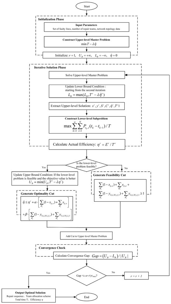
Since the lower-level model includes discrete operating states and generator startup constraints, it is difficult to derive conventional Benders cuts based on dual information. Therefore, a logic-based Integer L-shaped method is employed to solve the above bilevel model. In this method, the upper-level model is treated as the master problem, which is responsible for generating repair scheduling schemes, while the lower-level model serves as the subproblem, which optimizes the system restoration process under the given repair scheme.

The iterative solution procedure is described as follows:

Step a: Solve the upper-level master problem: The upper-level mixed-integer linear programming model is solved to obtain the decision variables at the current iteration, including the line-to-crew assignment x_ij,a, the repair sequence variable y_ol,ij, the start time S_ij and completion time C_ij of each line repair task, the total repair time T, and the estimated system restoration efficiency η.

Step b: Solve the lower-level subproblem: Based on the repair completion times C_ij provided by the upper-level model, the time-point sequence for the lower-level system restoration optimization model is constructed. The completion times obtained from the upper level are then passed to the lower level to determine the line operating status parameters and node connectivity parameters in each time period. By solving the lower-level model, the total restored energy supply and the actual restoration efficiency η are obtained.

Step c: Check the feasibility of the lower-level subproblem: The feasibility criterion for the lower-level model is defined as follows. If the lower-level optimization model can find a feasible solution satisfying all constraints, the subproblem is regarded as feasible. If the solver returns an “infeasible” termination condition, or an infeasibility exception is raised during the solution process, the subproblem is regarded as infeasible. If the subproblem is feasible, an optimality cut is added to the upper-level model. This cut implies that, when the upper-level solution deviates from the current solution, the estimated value of η should be adjusted accordingly. If the subproblem is infeasible, a feasibility cut is added to the upper-level model. This cut prevents the upper-level model from generating the same infeasible decision scheme again in subsequent iterations.

Step d: Update the upper and lower bounds: The upper bound is updated as follows. When the lower-level subproblem is feasible, the actual objective value f_actual^(r) is calculated. If f_actual^(r) < U_B, then the upper bound is updated as U_B = f_actual^(r). The upper bound represents the objective value of the best feasible solution found so far.

The lower bound is updated as follows. Starting from the second iteration, that is, after η is released from its fixed value, if the upper-level objective value f^(r) is greater than the current lower bound L_B, then the lower bound is updated as L_B = f^(r). The lower bound represents the optimal value of the relaxed upper-level problem with the accumulated cuts, and serves as a lower estimate of the optimal value of the original problem. Since η in the upper-level model is progressively driven toward its true value through the added cuts, η is fixed to zero in the first iteration, and the corresponding f^(r) does not have the meaning of a valid lower bound. Therefore, the lower bound is updated only from the second iteration onward.

The convergence gap is calculated as follows: Gap = (U_B − L_B)/|U_B|

Step e: Check convergence: The algorithm terminates and outputs the optimal solution when either of the following conditions is satisfied: (1) Gap ≤ ε, i.e., the gap between the upper and lower bounds meets the prescribed convergence tolerance; or (2) the rates of change in both T and η over consecutive iterations are below the specified thresholds, indicating that the solution has become stable. If convergence is not achieved, let r = r + 1 and return to Step a for the next iteration.

The detailed flowchart is shown in Figure 1.

Figure 1. Flowchart for Solving Bilevel Optimization Models via the Integer L-Shaped Method.

4. Case Study

To verify the effectiveness and practicality of the transmission line repair strategy proposed in this paper for post-ice-disaster scenarios, this section takes the modified IEEE 39-bus New England test system as a case study to analyze the established bi-level optimization model and the Integer L-shaped solution method.

4.1. Parameter Settings of the Ice Disaster Model

According to the Jones ice accretion thickness model and line failure probability model established in Section 2, the ice disaster scenario parameters in this case study are set as shown in Table 1. The disaster center is located at (500, 450), simulating the radial outward diffusion characteristics of an ice-rain disaster from this region.

Table 1. Parameters of the ice disaster scenario.

Parameter	Symbol	Value	Unit
Base freezing rain duration	Tbase	72	h
Base rainfall rate	Rbase	2.5	mm/h
Base wind speed	Vbase	4.5	m/s
Maximum disaster influence distance	Dmax	600	km
Conductor diameter	d	24	mm
Ice density	ρI	900	kg/m3
Water density	ρW	1000	kg/m3
Design load	aIW	35	N/m
Limit load	bIW	100	N/m
Disaster center coordinates	(xc, yc)	(500, 450)	-

Three repair teams are configured in this case study to participate in the de-icing work of outage lines, and all teams depart uniformly from Bus 14. The moving speed of the repair teams is set to 50 km/h.

4.2. Ice Disaster Scenarios and Fault Analysis

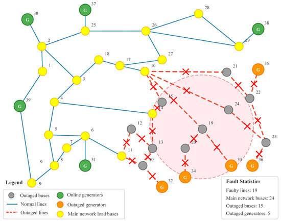
Based on the Jones ice accretion thickness calculation model and the exponential fault probability model, the ice accretion thickness and fault probability of each transmission line under the given ice disaster conditions are calculated. When the line fault probability exceeds the 95% threshold, the line is determined to require active outage to avoid subsequent risks. After calculation, a total of 19 high-risk lines are selected for active outage, and the line outage scenario under the rain, snow and freezing disaster is shown in Figure 2.

Figure 2. Line outage scenario under freezing rain, snow and ice disaster.

After the line outage, the system network topology changes. Due to the existence of power flow overload, voltage overload and other conditions, it is necessary to consider the active outage of part of the load to make the entire system meet various operating constraints. The statistical data of the system state after the line outage are shown in Table 2.

Table 2. Statistics of System State After Line Outage.

Statistical Indicators	Value
Number of Faulty Lines	19 transmission lines
Number of Main Network Buses	24 buses
Number of Outaged Buses	15 buses
Total System Load	6914 MW
Main Network Load	4004 MW
Outage Load	2039 MW
Outage Ratio	29.50%
Online Generators	30, 31, 37, 38, 39
Online Generation Capacity	4215 MW
Outaged Generators	32, 33, 34, 35, 36
Outaged Generation Capacity	3152 MW

From the perspective of generation-load balance, the current online generation capacity of the main network is 4215 MW, while the main network load is only 4004 MW, indicating a large power margin. This shows that the main network has the ability to supply power to the restoration area, and the optimization focus of the repair strategy is to restore key lines as soon as possible through a reasonable repair sequence, so that the outage load can regain power supply.

4.3. Model Optimization Solution and Analysis

The logic-based Integer L-shaped method is adopted to solve the bi-level optimization model. This method coordinates the upper-level repair scheduling and lower-level system operation restoration through an iterative approach, gradually approaching the optimal solution. Table 3 records the iterative solution process of the algorithm.

Table 3. Algorithmic Iterative Solution Process.

Iteration	T (h)	Estimated η	Actual η	Gap (%)
1	20.85	0	3580	∞
2	21.08	3659	3826	17.10
3	21.15	3955	4056	8.00
4	21.18	4080	4122	3.10
5	21.21	4150	4175	1.20

It can be seen from Table 3 that the algorithm converges after 5 iterations, with a final convergence Gap of 1.2%, which meets the preset convergence tolerance requirement of 2%. During the iteration process:

In the 1st iteration, the upper-level model initializes the estimated efficiency value η to 0 and solves for the initial repair scheduling scheme. This scheme is transmitted to the lower-level model for system operation optimization, and the actual restoration efficiency is obtained as 3580 MW. Based on this, the first optimality cut is generated and added to the upper-level model.

In the 2nd to 4th iterations, with the continuous accumulation of optimality cuts, the estimated value of restoration efficiency by the upper-level model gradually approaches the actual calculated value of the lower-level model. The estimated η value gradually increases from 3659 MW to 4080 MW, and the deviation from the actual value gradually decreases; the Gap decreases from 17.1% to 8.0% and 3.1% in turn.

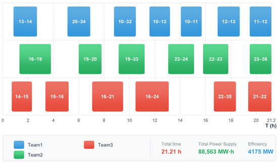
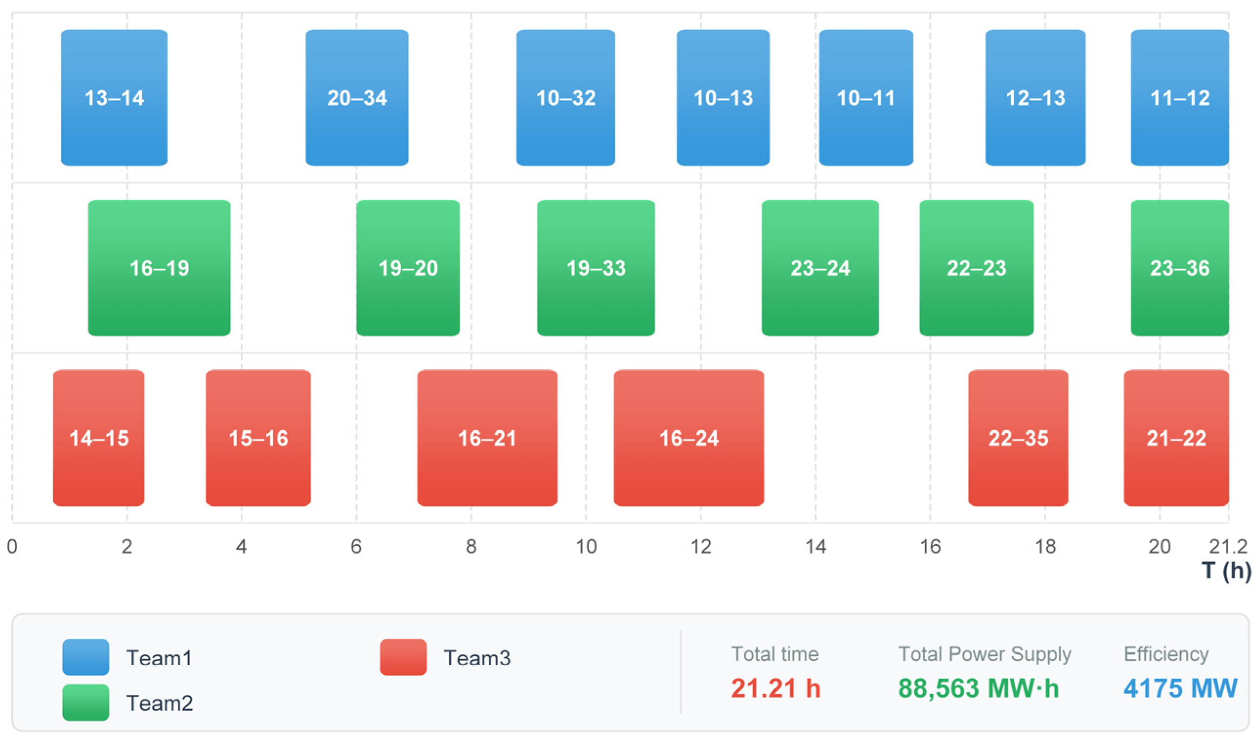
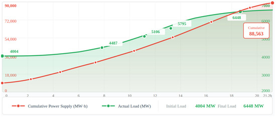
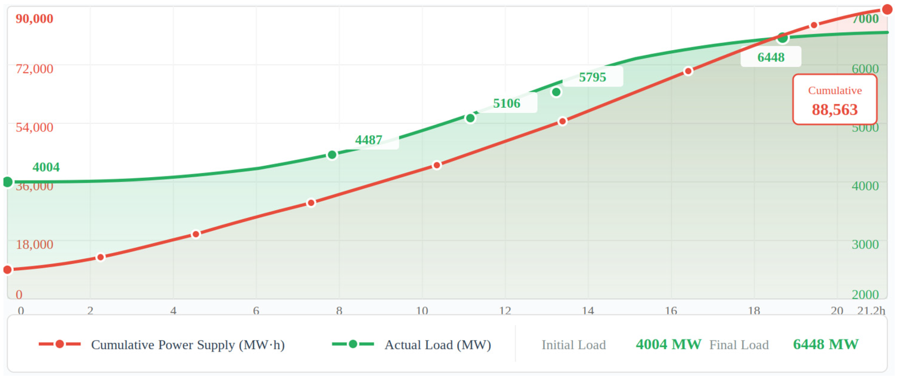
In the 5th iteration, the estimated efficiency value η = 4150 MW is very close to the actual value of 4175 MW, the upper and lower bounds further approach, and the Gap drops to 1.2%, meeting the convergence condition, and the algorithm terminates. Finally, the optimal solution is obtained: total repair time T = 21.21 h, system restoration efficiency η = 4175 MW, and total power supply E = 88,563 MW·h.

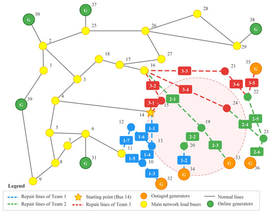
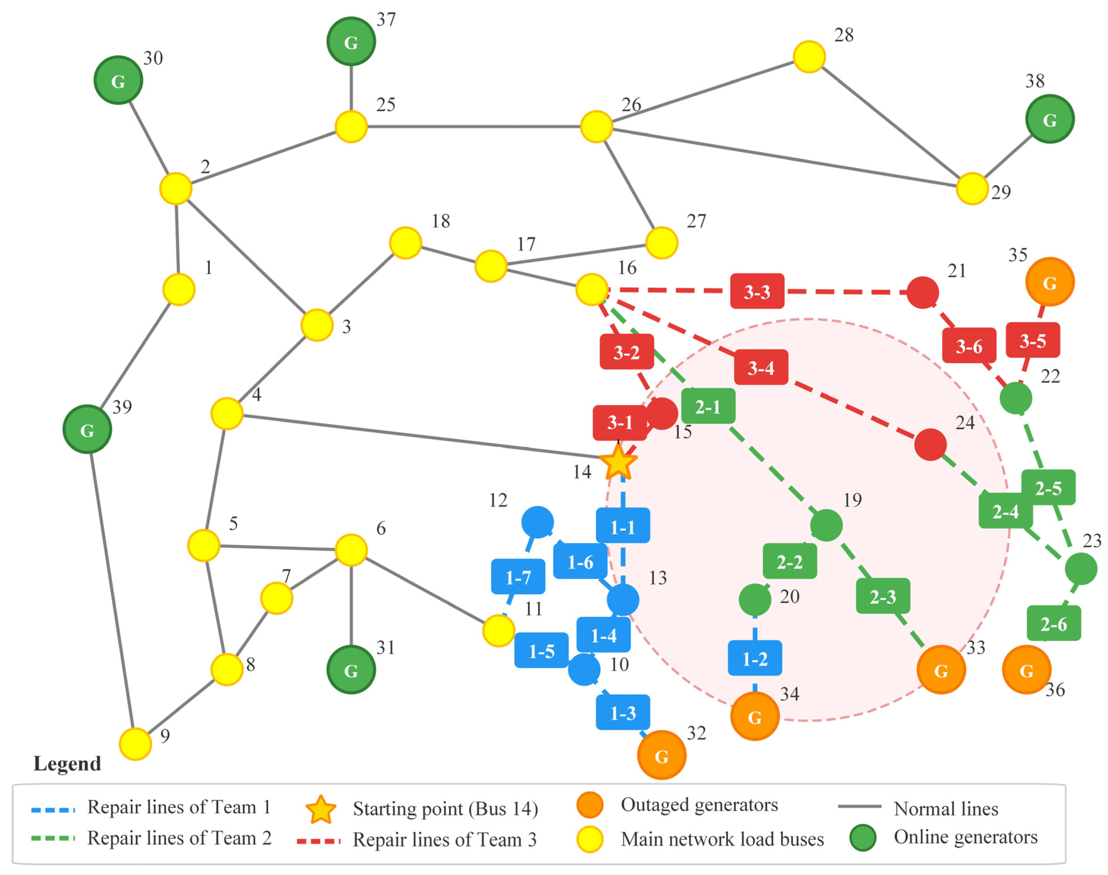
Based on the above solution results, the optimal task allocation scheme for the 3 repair teams is shown in Table 4, and the repair scheme of each team can also be intuitively seen from Figure 3.

Table 4. Repair Team Allocation Scheme.

Team	Repair Line Sequence
1	13–14→20–34→10–32→10–13→10–11→12–13→11–12
2	16–19→19–20→19–33→23–24→22–23→23–36
3	14–15→15–16→16–21→16–24→22–35→21–22

Figure 3. Path planning diagram of repair teams.

The repair team path planning chart and the repair task Gantt chart are shown in Figure 3 and Figure 4. It can be seen from them that the optimization results give priority to restoring the boundary lines directly connected to the main network (such as 14–15, 15–16, 11–12, etc.), and then gradually expand to the periphery. The key lines connected to the outage generators (10–32, 19–33, 20–34, 22–35, 23–36) are successively repaired in the middle and later stages, enabling the outage generators to be connected to the grid in sequence and gradually improving the system power supply capacity.

Figure 4. Gantt chart of repair tasks for each team.

Under the optimal repair scheme, the lower-level model optimizes the system operation state. Figure 5 shows the system load restoration curve during the repair process.

Figure 5. Grid restoration process analysis diagram.

It can be observed from Figure 5 that the system load restoration exhibits an obvious stepwise growth characteristic, which is closely related to the sequential restoration of faulty lines and the gradual grid connection of outaged generators. At the initial stage of repair, the system load remains at the initial level since the lines have not been fully restored. With the restoration of key lines, some outaged buses are reconnected to the main network, and the system load begins to rise. In the middle stage of repair, as the lines connected to generators are successively repaired, the outaged generators start to be connected to the grid, and the power supply capacity of the system is significantly improved. In the late stage of repair, all remaining generators are connected to the grid, and the system load recovers to a level close to that before the disaster.

4.4. Example Analysis

To verify the effectiveness of the proposed bilevel coordinated optimization method, this section designs comparative schemes from two perspectives. First, schemes with different objective preferences are compared to demonstrate the necessity of balancing multiple objectives. Second, non-coordinated benchmark schemes are introduced to verify the superiority of the bilevel coordinated optimization framework itself. Specifically, the following five schemes are considered:

Scheme A (proposed method): a bilevel optimization model that jointly considers repair time and system load restoration efficiency.

Scheme B (efficiency-oriented): maximization of system load restoration efficiency only.

Scheme C (time-oriented): minimization of total repair time only.

Scheme D (independent optimization scheduling): the upper-level repair scheduling model is first solved independently, with the sole objective of minimizing total repair time and without considering feedback from the lower-level restoration efficiency. After a fixed repair sequence is obtained, it is passed to the lower level as a known input, and only the system restoration optimization problem is solved. In this scheme, no iterative feedback mechanism exists between the upper and lower levels.

Scheme E (nearest-dispatch heuristic): the repair sequence is independently determined using a nearest-dispatch heuristic rule, under which each crew always selects the nearest unrepaired line from its current location. The resulting fixed repair sequence is then passed to the lower-level model for system restoration optimization. This scheme represents a commonly used experience-based repair strategy in engineering practice.

A comparison of the restoration performance of the five schemes is presented in Table 5.

Table 5. Recovery Performance Comparison of Different Schemes.

Scheme	Strategy Description	T (h)	η (MW)
Scheme A	Proposed Bi-level Optimization Method	21.21	4175
Scheme B	Efficiency-oriented	23.31	4340
Scheme C	Time-oriented	20.85	3580
Scheme D	Independent optimization scheduling	21.08	3659
Scheme E	Nearest-dispatch heuristic	23.52	4028

(1)

Necessity of the coordinated optimization framework

Schemes D and E are adopted as two non-coordinated benchmarks to demonstrate the necessity of the proposed bilevel coordinated optimization framework from different perspectives.

Scheme D employs the same upper-level repair scheduling model as Scheme A, but without iterative feedback between the upper and lower levels. As shown in Table 5, Schemes A and D yield nearly the same total repair time; however, the restoration efficiency η of Scheme A reaches 4175 MW, representing a 14.1% improvement over the 3659 MW obtained by Scheme D, while the total restored energy supply is increased by 14.8%. This result indicates that, under nearly identical repair durations, the bilevel coordinated iterative mechanism can significantly improve system load restoration performance by adjusting the repair sequence. Further analysis of the difference in repair sequences shows that, in Scheme D, the repair crews prioritize internal lines in areas close to their starting locations, whereas in Scheme A, through lower-level feedback, “perceives” that key lines connected to out-of-service generators (such as lines 20–34, 10–32, and 19–33) contribute more significantly to system restoration efficiency. Therefore, the repair sequence is appropriately adjusted to prioritize the restoration of these critical lines, enabling the out-of-service generators to be reconnected to the grid at an earlier stage.

Scheme E represents a common experience-based strategy in engineering practice. As shown in Table 5, the total repair time of Scheme E is 23.52 h, which is approximately 2.3 h longer than that of Scheme A, while its restoration efficiency is η = 4028 MW, lower than the 4175 MW achieved by Scheme A. This indicates that the proposed method can substantially shorten the repair time while still maintaining a higher restoration efficiency, thereby achieving a coordinated improvement in both repair duration and restoration performance.

The above two sets of comparisons jointly verify the necessity of the bilevel coordinated optimization framework from complementary perspectives. The comparison between Schemes A and D demonstrates the significant role of the coordinated iterative mechanism in improving restoration efficiency, whereas the comparison between Schemes A and E confirms the clear advantage of the coordinated optimization framework in reducing repair time.

(2)

Superiority of multi-objective balancing

Scheme B is efficiency-oriented, achieving a restoration efficiency of η = 4340 MW; however, its total repair time increases to 23.31 h, which is about 2.1 h longer than that of Scheme A. Scheme C is time-oriented and yields the shortest total repair time, but its restoration efficiency is only 3580 MW, which is 14.2% lower than that of Scheme A.

By simultaneously considering repair time and restoration efficiency in the upper-level objective function, the proposed method improves restoration efficiency as much as possible while maintaining a satisfactory repair duration, thereby demonstrating the advantage of multi-objective coordinated optimization in terms of overall restoration performance.

In summary, the comparisons of Scheme A with Schemes D and E confirm the necessity of the bilevel coordinated mechanism itself, while the comparisons of Scheme A with Schemes B and C verify the superiority of the multi-objective balancing strategy. The proposed method can effectively improve the system load restoration level while taking repair efficiency into account.

5. Conclusions

This paper proposes a coordinated optimization method for transmission line repair and system restoration in response to snow- and ice-related disasters. To address the problem of large-scale transmission line outages under extreme icing conditions, a transmission line failure probability model considering the spatial distribution characteristics of the disaster is established. On this basis, a bilevel optimization model is developed with the objective of minimizing total repair time while accounting for load restoration efficiency, and a logic-based Integer L-shaped method is employed for its solution. Case studies based on the IEEE 39-bus system demonstrate that:

(1)

Under an ice-disaster scenario involving 19 out-of-service lines and 29.5% load interruption, the proposed method converges within five iterations and obtains an optimal scheme with a total repair time of 21.21 h and a restoration efficiency of 4175 MW, while the total restored energy supply reaches 88,563 MW·h.

(2)

Comparisons with non-coordinated benchmark schemes verify the necessity of the bilevel coordinated framework. Under nearly identical total repair times, the coordinated iterative mechanism improves restoration efficiency by 14.1%; under comparable restoration efficiency levels, the coordinated optimization framework reduces the total repair time by approximately 2.3 h.

(3)

Compared with time-oriented and efficiency-oriented strategies, the proposed method exhibits clear advantages in terms of overall restoration performance, achieving relatively short repair times while maintaining high load restoration efficiency.

It should also be noted that the current study has several limitations. Specifically, the proposed method assumes that the number and initial location of repair crews are predetermined and that no secondary failures occur during the repair process, which may not fully reflect certain real-world operating conditions. In this study, a unified disaster intensity coefficient is used to linearly scale the meteorological parameters, based on the assumption that the spatial distributions of meteorological variables are coordinated within a freezing-rain weather system. In future work, differentiated attenuation models may be introduced in combination with numerical weather prediction data to further improve the accuracy of scenario construction. In addition, the current model treats all transmission-level loads equally. In future work, load importance weighting or differentiated load-shedding costs may be introduced to better capture the priority of critical loads at the transmission level, further improving the engineering relevance of the proposed model.

References

- Zhou, B.; Gu, L.; Ding, Y.; Shao, L.; Wu, Z.; Yang, X.; Li, C.; Li, Z.; Wang, X.; Cao, Y.; et al. The great 2008 Chinese ice storm: Its socioeconomic-ecological impact and sustainability lessons learned. Bull. Am. Meteorol. Soc. 2011, 92, 47–60. [Google Scholar] [CrossRef] [Scilit]
- Dong, Q.; Chen, B.; Hu, N.; Kong, L.; Chen, T.; Wang, J.; Zhang, B. Comparison of two widespread snow and ice weather events in China in February 2024. J. Appl. Meteorol. Sci. 2024, 35, 385–399. (In Chinese) [Google Scholar]
- Lin, J.H.; Wu, Y.K. Review of power system resilience concept, assessment, and enhancement measures. Appl. Sci. 2024, 14, 1428. [Google Scholar] [CrossRef] [Scilit]
- Zhang, Z.; Zhang, H.; Yue, S.; Zeng, W. A review of icing and anti-icing technology for transmission lines. Energies 2023, 16, 601. [Google Scholar] [CrossRef] [Scilit]
- Li, Q.; Li, P.; Zhang, Q.; Ren, W.; Cao, M.; Gao, S. Icing load prediction for overhead power lines based on SVM. In Proceedings of the 2011 International Conference on Modelling, Identification and Control, Shanghai, China, 26–29 June 2011; pp. 104–108. [Google Scholar] [CrossRef] [Scilit]
- He, L.; Luo, J.; Zhou, X. A novel deep learning model for transmission line icing thickness prediction. In Proceedings of the 2021 IEEE 5th Advanced Information Technology, Electronic and Automation Control Conference (IAEAC), Chongqing, China, 12–14 March 2021; pp. 733–738. [Google Scholar] [CrossRef] [Scilit]
- Wang, Y.; Wei, S.; Yin, F.; Yang, Y.; Tan, L.; Cao, W. Review on key technology of de-icing robot running on overhead transmission line. J. Mech. Eng. 2011, 47, 30–38. (In Chinese) [Google Scholar] [CrossRef] [Scilit]
- Huang, W.; Hu, B.; Shahidehpour, M.; Sun, Y.; Sun, Q.; Yan, M.; Shao, C.; Xie, K. Preventive scheduling for reducing the impact of glaze icing on transmission lines. IEEE Trans. Power Syst. 2022, 37, 1297–1310. [Google Scholar] [CrossRef] [Scilit]
- Lu, J.; Guo, J.; Jian, Z.; Yang, Y.; Tang, W. Resilience assessment and its enhancement in tackling adverse impact of ice disasters for power transmission systems. Energies 2018, 11, 2272. [Google Scholar] [CrossRef] [Scilit]
- Zhao, N.; Yu, X.; Hou, K.; Liu, X.; Mu, Y.; Jia, H.; Wang, H.; Wang, H. Full-time scale resilience enhancement framework for power transmission system under ice disasters. Int. J. Electr. Power Energy Syst. 2021, 129, 106609. [Google Scholar] [CrossRef] [Scilit]
- Lai, Y.; Sun, Z.; Lu, Z.; Liu, Q. Power grid optimization operation and resilience improvement strategy considering the participation of energy storage resource aggregation. Electr. Power 2025, 58, 57–65. [Google Scholar]
- Zhang, H.; Li, G.; Yuan, H. Collaborative optimization of post-disaster damage repair and power system operation. Energies 2018, 11, 2611. [Google Scholar] [CrossRef] [Scilit]
- Tan, Y.; Qiu, F.; Das, A.K.; Kirschen, D.S.; Arabshahi, P.; Wang, J. Scheduling post-disaster repairs in electricity distribution networks. IEEE Trans. Power Syst. 2019, 34, 2611–2621. [Google Scholar] [CrossRef] [Scilit]
- Arif, A.; Wang, Z.; Wang, J.; Chen, C. Power distribution system outage management with co-optimization of repairs, reconfiguration, and DG dispatch. IEEE Trans. Smart Grid 2018, 9, 4109–4118. [Google Scholar] [CrossRef] [Scilit]
- Lei, S.; Chen, C.; Li, Y.; Hou, Y. Resilient disaster recovery logistics of distribution systems: Co-optimize service restoration with repair crew and mobile power source dispatch. IEEE Trans. Smart Grid 2019, 10, 6187–6202. [Google Scholar] [CrossRef] [Scilit]
- Laporte, G.; Louveaux, F.V. The integer L-shaped method for stochastic integer programs with complete recourse. Oper. Res. Lett. 1993, 13, 133–142. [Google Scholar] [CrossRef] [Scilit]
- Wu, X.; Zhang, G. Ice and snow disaster on the electric power grid and preventive measures. Electr. Power 2008, 41, 14–18. (In Chinese) [Google Scholar]
- Jones, K.F. A simple model for freezing rain ice loads. Atmos. Res. 1998, 46, 87–97. [Google Scholar] [CrossRef] [Scilit]
- Krishnasamy, S.G. Assessment of weather induced transmission line loads on a probabilistic basis. IEEE Trans. Power Appar. Syst. 1985, 104, 2510–2516. [Google Scholar]
- Feng, W. Operation Risk Assessment on Power Grid in Ice Storm and Network Protection. Master’s Thesis, Harbin Institute of Technology, Harbin, China, 2014. (In Chinese) [Google Scholar]
- Liu, X.; Hou, K.; Jia, H.; Zhao, J.; Mili, L.; Jin, X.; Wang, D. A planning-oriented resilience assessment framework for transmission systems under typhoon disasters. IEEE Trans. Smart Grid 2020, 11, 5431–5441. [Google Scholar] [CrossRef] [Scilit]
- Liu, S.; Chen, C.; Jiang, Y.; Lin, Z.; Wang, H.; Waseem, M.; Wen, F. Bi-Level Coordinated Power System Restoration Model Considering the Support of Multiple Flexible Resources. IEEE Trans. Power Syst. 2023, 38, 1583–1595. [Google Scholar] [CrossRef] [Scilit]
- Sun, L.; Wang, H.; Li, M.; Wei, Y.; Lin, Z. Bi-level Generator Start-up Sequence Optimization Model for Power System Restoration Considering the DoS Attack. Int. J. Electr. Power Energy Syst. 2024, 162, 110219. [Google Scholar] [CrossRef] [Scilit]
- Lu, H.; Zhang, H.; Chen, X.; Zhou, S. Collaborative Planning Method for Multi-energy Networks Based on Double-layer Game Theory. Electr. Power 2025, 58, 93–99. (In Chinese) [Google Scholar]
Disclaimer/Publisher’s Note: The statements, opinions and data contained in all publications are solely those of the individual author(s) and contributor(s) and not of MDPI and/or the editor(s). MDPI and/or the editor(s) disclaim responsibility for any injury to people or property resulting from any ideas, methods, instructions or products referred to in the content. |
© 2026 by the authors. Licensee MDPI, Basel, Switzerland. This article is an open access article distributed under the terms and conditions of the Creative Commons Attribution (CC BY) license.