TLA-SleepNet: A Transformer–BiLSTM–Attention Network for Automatic Sleep Staging Using Single-Channel Ballistocardiogram Signals

Abstract

Traditional sleep staging studies typically rely on signals collected using contact-based sensors, which may interfere with the natural sleep state of subjects and thus affect the authenticity and reliability of the recorded data. To address this limitation, this study proposes an automatic sleep staging method based on non-contact single-channel ballistocardiogram (BCG) signals. First, band-pass filtering is applied to the raw BCG signals to separate the heart rate and respiratory components. Heart rate variability (HRV) and respiratory rate variability (RRV) features are then extracted, and mutual information is used to select key feature subsets that exhibit strong correlations with different sleep stages. Considering the complexity and prominent temporal characteristics of real-world sleep data, a temporal modeling network named TLA-SleepNet is constructed to enhance the model’s capability in capturing complex sequential features and improving robustness. Experiments conducted on 10 independent sleep recordings containing a total of 10,614 sleep epochs demonstrate that, under subject non-independent testing conditions with five-fold cross-validation, the proposed method achieves an accuracy of 87.1% in the sleep staging task, with precision, kappa coefficient, and F1-score reaching 92.4%, 81.9%, and 88.7%, respectively. The results indicate that the proposed method can achieve a reliable sleep staging performance without direct contact between sensors and the human body, providing a feasible solution for non-contact sleep monitoring in home-based and mobile healthcare applications.

1. Introduction

Sleep is an essential physiological activity for humans. Long-term sleep deprivation can impair cognitive function and increase the risk of various chronic diseases. Clinically, sleep quality is usually evaluated according to physiological characteristics observed in different sleep stages. Accurate identification of sleep stages is therefore important for sleep assessment and clinical diagnosis. In most sleep studies, sleep staging is performed using 30 s epochs. According to the latest scoring criteria of the American Academy of Sleep Medicine (AASM), sleep is classified into wake (WK), rapid eye movement (REM), and non-rapid eye movement (NREM) stages [1]. The NREM stage is further divided into N1, N2, and N3.

Polysomnography (PSG) is currently regarded as the gold standard for evaluating sleep architecture [2]. PSG simultaneously records multiple physiological signals, including electroencephalogram (EEG), electrooculogram (EOG), electromyography (EMG), blood oxygen saturation, airflow, and respiratory signals. It is widely used for the clinical diagnosis of sleep disorders. However, PSG requires multiple electrodes and sensors attached to the human body. These sensors may disturb natural sleep and reduce comfort. In addition, PSG systems are expensive and difficult to deploy in home environments. Consequently, recent studies have increasingly focused on low-cost and comfortable sleep staging approaches based on single-channel physiological signals.

Current research on sleep staging has developed along several directions. Among them, contact-based physiological signal methods have been widely investigated. Chen Lingling analyzed multi-band EEG features and proposed a residual sleep network (RSNSleepNet) for automatic sleep staging, achieving an accuracy of 85% [3]. Du-Yan extracted eye-movement features from EOG signals using wavelet packet transform and applied a convolutional neural network (CNN) model [4], achieving an accuracy above 91.72% in a four-class classification task. Habibprocessed photoplethysmography (PPG) signals using CNNs and achieved accuracies of 96.30%, 95.96%, and 93.60% in two-, three-, and four-class classification tasks, respectively [5]. In ECG-based studies, Wang extracted heart rate variability (HRV) features and used a gradient boosting decision tree (GBDT) model [6], achieving a sleep staging accuracy of 82%. These studies demonstrate that different single-channel contact-based physiological signals contain useful information related to sleep stages. However, these approaches still have limitations in terms of comfort and long-term continuous monitoring.

In recent years, non-contact sleep staging methods have attracted increasing attention. Doppler continuous wave radar can monitor respiration, heartbeat, and body micro-movements by detecting frequency shifts in reflected signals. Rahman et al. achieved an accuracy of 89.6% in the classification of REM/NREM and wake states, and 80.2% in REM versus NREM classification [7]. Studies based on wireless fidelity (Wi-Fi) signals extract physiological features using channel state information and received signal strength indicators. Yu et al. combined these features with a CNN-LSTM model and achieved an accuracy of 81.8% in a four-class sleep staging task [8]. Ultra-wideband radar can detect respiration, heart rate, and micro-movement signals with high temporal resolution. Li et al. achieved an accuracy of 81.1% in a four-class sleep staging task using UWB radar signals [9]. These studies demonstrate the feasibility of radar- and wireless-based sleep monitoring. Recent studies have explored system-level non-contact biosignal monitoring using alternative physiological signals [10]. However, such systems are sensitive to environmental interference and body position changes. Their ability to detect subtle physiological signals is limited, which may reduce the accuracy of REM and NREM classification and restrict their application in home sleep monitoring. Recent advances in embedded biomedical acquisition systems have further demonstrated the importance of integrated sensing and edge processing architectures for robust physiological signal monitoring [11].

Ballistocardiogram (BCG) signals represent a physiological measurement method that reflects cardiac activity through body micro-movements. Unlike traditional sensing techniques, BCG signal acquisition is non-invasive and does not require direct contact between the human body and electrodes or sensors. In medical research, BCG signals are often used to study cardiovascular function and related heart diseases. The “IJK” waveform complex in BCG signals corresponds to the “QRS” complex in electrocardiogram signals, and the J-peak corresponds to the R-peak, which can be used to calculate heartbeat intervals [12]. By analyzing BCG signals, HRV features can be extracted for sleep staging studies. In addition, BCG signals contain abundant respiratory information. By separating the respiratory component from the raw BCG signal, respiratory rate variability (RRV) features can be extracted to provide additional information for sleep stage classification [13].

Previous studies have verified the feasibility of using BCG signals for sleep staging. Jing Jianmeng collected BCG signals using piezoelectric vibration sensors and applied a linear-chain conditional random field model [14], achieving classification accuracies of 76.4%, 69.1%, and 61.8% in three-, four-, and five-stage sleep classification tasks. Luo Yi et al. used P(VDF-TrFE)/PZT piezoelectric sensors to acquire BCG signals and applied a support vector machine (SVM) model, achieving an accuracy of 72.5% in four-stage sleep classification [15]. Yi et al. extracted HRV and RRV features from BCG signals and used SVM for three-stage sleep classification, achieving an accuracy of 74% [16]. Ahmed et al. introduced a one-dimensional convolutional neural network (1D-CNN) to model BCG signals and achieved a classification accuracy above 94% in a binary sleep staging task. These studies demonstrate the advantages of deep learning in capturing temporal features from BCG signals [17].

Although previous studies have made progress in sleep staging using single-channel BCG signals, most existing methods rely on convolutional networks or simple recurrent neural networks. These models mainly focus on local short-term features and have difficulty modeling complex long-term temporal dependencies in BCG signals. They also struggle to capture both short-term fluctuations and long-term temporal trends. Moreover, they often fail to emphasize critical temporal segments during sleep staging.

To address these limitations, this study proposes a TLA-SleepNet model based on Transformer, bidirectional long short-term memory (BiLSTM), and an attention mechanism. The Transformer component captures global temporal dependencies, while the BiLSTM models local temporal dynamics. The attention mechanism highlights key temporal features during sleep staging. This hybrid architecture improves temporal feature representation and enhances sleep stage classification performance. Experimental results on a BCG dataset demonstrate the effectiveness and robustness of the proposed method.

The main contributions of this study are summarized as follows:

1. A non-contact automatic sleep staging framework based on single-channel BCG signals is proposed for unobtrusive sleep monitoring.

2. HRV and RRV features are extracted from BCG signals, and mutual information is used to select discriminative physiological features.

3. A hybrid deep learning model, TLA-SleepNet, integrating Transformer, BiLSTM, and attention mechanisms, is designed to model temporal dependencies in sleep data.

4. Experiments conducted on real sleep datasets demonstrate that the proposed method achieves a reliable performance in sleep stage classification.

2. Preprocessing

2.1. Overview

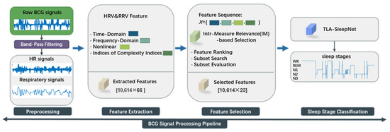
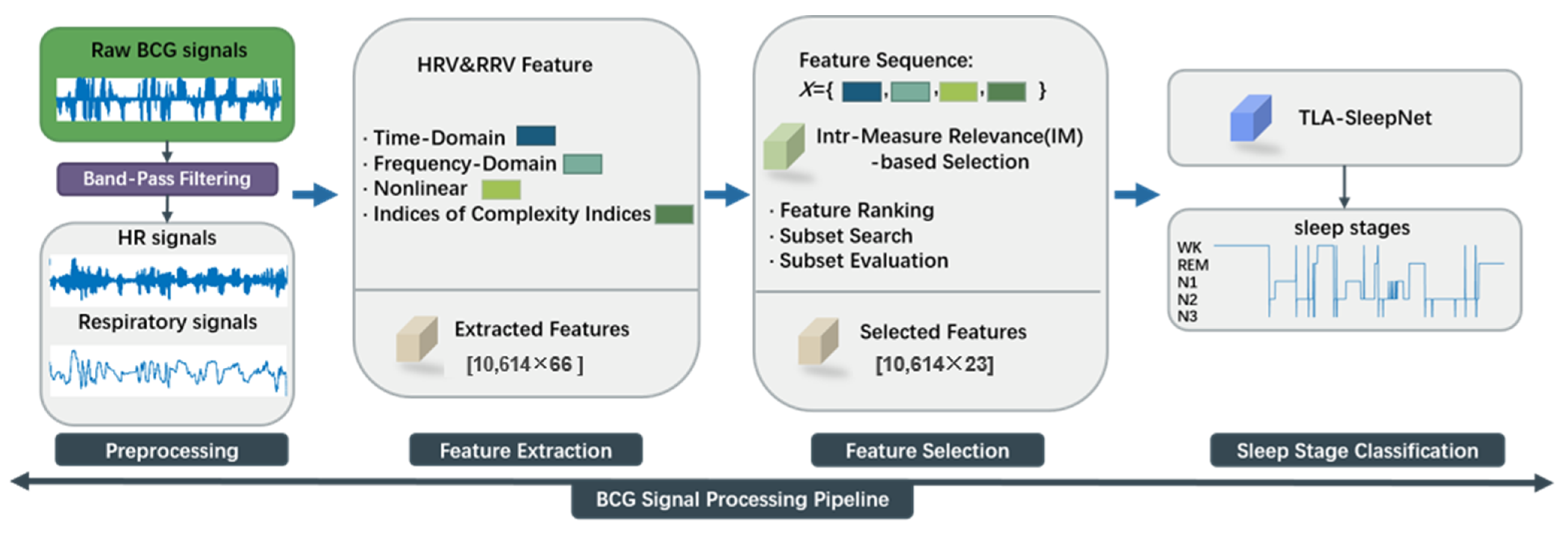
The framework of the proposed method is illustrated in Figure 1 and consists of three main components.

Figure 1. Process Overview.

(1) A band-pass filter (BPF) is applied to select specific frequency bands and separate cardiac and respiratory signals from the raw BCG signals [18]. The signals are then segmented into 30 s epochs. Feature peak positions are extracted to calculate first-order differences, forming the JJi and BBi sequences.

(2) Based on the JJi and BBi sequences, multidimensional HRV and RRV features are initially extracted. Subsequently, the features are reduced using a mutual information (MI) algorithm [19] to remove noise and redundant information, thereby enhancing the validity and reliability of the feature representation.

(3) A TLA-SleepNet architecture is proposed, which integrates global, local, and key-time modeling. This structure enables collaborative learning of multiscale features from BCG physiological signals for accurate sleep stage classification.

2.2. Signal Processing

BCG signals originate from subtle body movements and the mechanical activity of the heart. Therefore, they are influenced not only by inter-individual differences but also by temporal variations within the same subject. These characteristics pose challenges for building effective temporal representation models. In addition, noise introduced during the signal acquisition process may contaminate the BCG signals and even mask useful physiological information, which can degrade data quality [20].

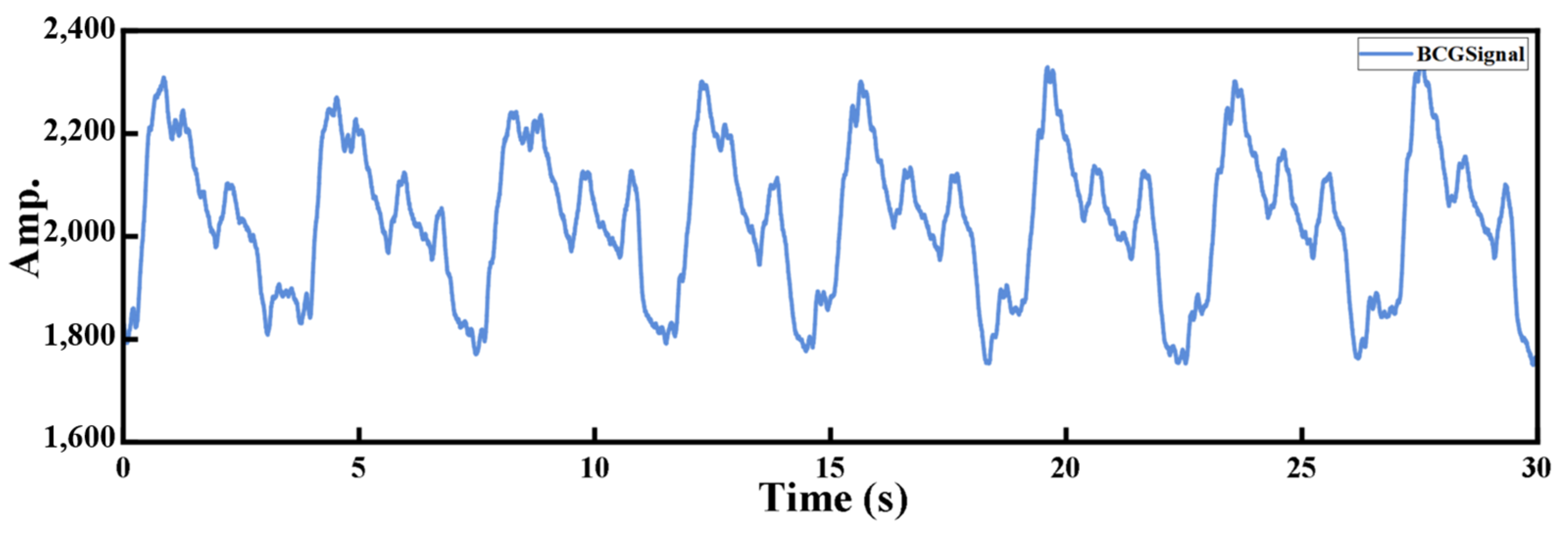
The BCG signal, as illustrated in Figure 2, contains an “IJK” waveform complex that reflects cardiac activity. By detecting the J-peak and calculating the first-order difference, the heartbeat interval can be obtained for heart rate variability analysis.

Figure 2. Raw BCG signal waveform.

Since raw BCG signals typically contain both cardiac and respiratory components, BPF is applied in this study to separate these two components.

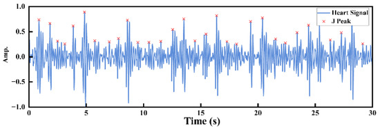
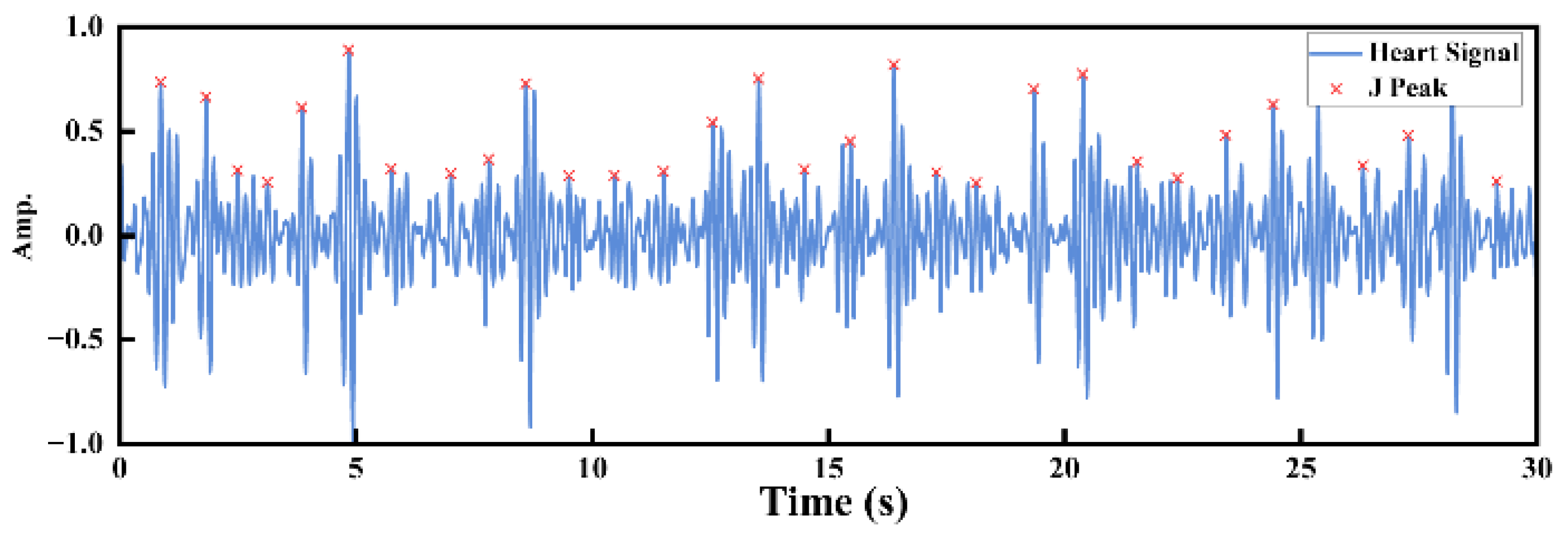
For a normal heart rate range (60–100 bpm), the passband of the BPF is set to 0.6667–4 Hz to remove respiratory components and high-frequency noise, thereby obtaining the cardiac waveform. To enhance the adaptability of the algorithm to heartbeat amplitude variations among different subjects, the signal is normalized and processed with half-wave rectification (retaining only the positive half-cycle) to eliminate the influence of negative values. Subsequently, the signal segment 0.4 s after each J-peak is dynamically segmented, and peaks with time intervals not less than 0.8 s are extracted [21], as shown in Figure 3.

Figure 3. Visualization of feature peak extraction from the heart rate signal.

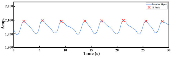
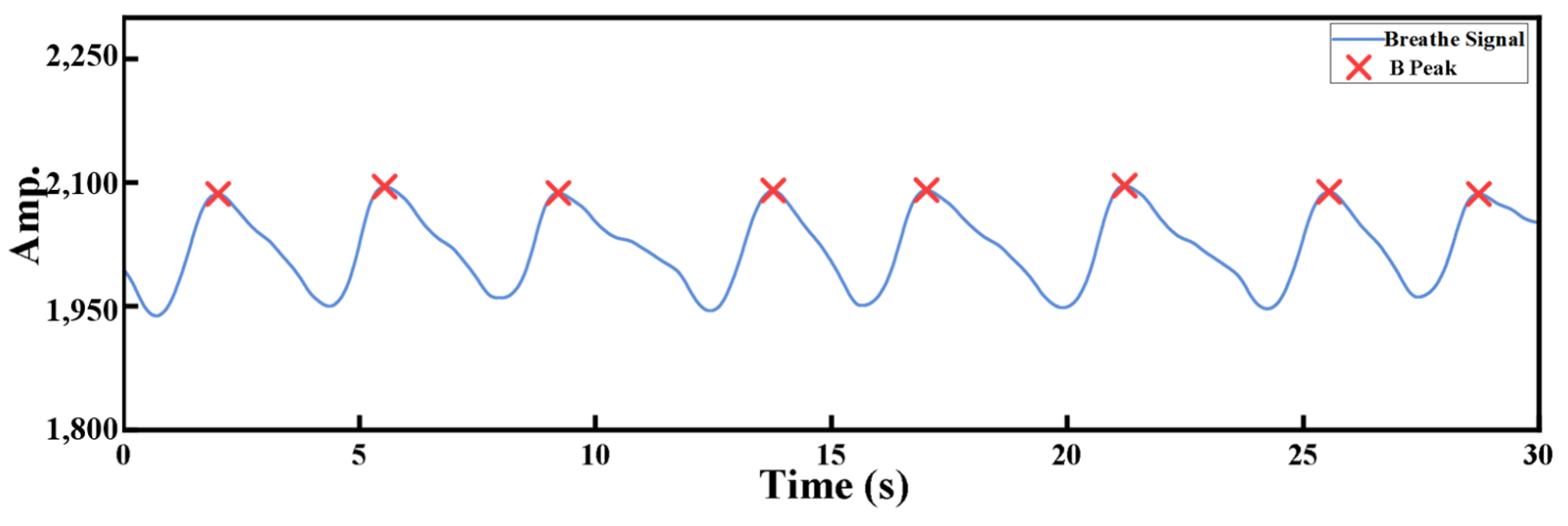
For a normal respiratory rate (12–20 breaths/min), the passband of the BPF is set to 0.1333–0.5 Hz to extract a clear respiratory signal [22]. As shown in Figure 4, by setting appropriate cutoff frequencies, irrelevant components can be effectively filtered out, thereby isolating a clear respiratory signal.

Figure 4. Visualization of feature peak extraction from the respiratory signal.

2.3. Feature Extraction

2.3.1. Time-Domain Features

Time-domain features [23] reflect variations in heart rate and respiration within a specific time interval through statistical analysis. In particular, the variations in the BBi interval (the first-order difference in respiratory signal peaks) and the JJi interval (the first-order difference in cardiac signal peaks) can intuitively evaluate respiratory and heart rate variability. The time-domain feature extraction and calculation methods used in this study are described as follows:

RMSSD represents the root mean square of successive differences between adjacent feature peak intervals, quantifying short-term variability in the interval series:

$$\mathrm{R}\mathrm{M}\mathrm{S}\mathrm{S}\mathrm{D}=\sqrt{{\displaystyle \frac{1}{N-1}}{\sum }_{i=1}^{N-1}(X{X}_{i+1}-X{X}_i{)}^2}$$

(1)

SDNN represents the standard deviation of the intervals between successive feature peaks, reflecting overall variability in the interval series:

$$\mathrm{S}\mathrm{D}\mathrm{N}\mathrm{N}=\sqrt{{\displaystyle \frac{1}{N}}{\sum }_{i=1}^{N-1}(X{X}_{i+1}-mean(XX){)}^2}$$

(2)

SDSD represents the standard deviation of the first-order differences in successive feature peak intervals, reflecting short-term variability in the interval series:

$$\mathrm{S}\mathrm{D}\mathrm{S}\mathrm{D}=\sqrt{{\displaystyle \frac{1}{N-2}}{\sum }_{i=1}^{N-1}(\Delta X{X}_i-\overline{\Delta \mathrm{X}X}{)}^2}$$

(3)

CVNN reflects the degree of variability of the intervals between successive feature peaks relative to their mean value, expressed as a percentage:

$$\mathrm{C}\mathrm{V}\mathrm{N}\mathrm{N}={\displaystyle \frac{\mathrm{S}\mathrm{D}\mathrm{N}\mathrm{N}({XX}_i)}{\mathrm{M}\mathrm{e}\mathrm{a}\mathrm{n}({XX}_i)}}$$

(4)

CVSD reflects the degree of variability of the standard deviation of successive feature peak intervals relative to their mean value:

$$\mathrm{C}\mathrm{V}\mathrm{S}\mathrm{D}={\displaystyle \frac{\mathrm{R}\mathrm{M}\mathrm{S}\mathrm{S}\mathrm{D}(X{X}_i)}{\mathrm{M}\mathrm{e}\mathrm{a}\mathrm{n}(X{X}_i)}}$$

(5)

where XX_i represents the deviation on the x-axis of the current feature peak in the heart rate interval sequence JJi or the respiratory interval sequence BBi, while XX denotes the deviations of all feature peaks in JJi and BBi. Additionally, Mean, Max, and Min represent the mean, median, mode, maximum, minimum, and median absolute deviation of the JJi and BBi sequences.

pNN50 and pNN20 represent the percentage of successive feature peak intervals that differ by more than 50 ms and 20 ms, respectively:

$$\mathrm{p}\mathrm{N}\mathrm{N}50={\displaystyle \frac{1}{N-1}}{\sum }_{i=1}^{N-1}I(|X{X}_{i+1}-X{X}_i|>50)$$

(6)

$$p_{NN20}={\displaystyle \frac{1}{N-1}}{\sum }_{i=1}^{N-1}I(|X{X}_{i+1}-X{X}_i|>20)$$

(7)

where XX_i denotes the deviation on the x-axis of the current feature peak in the heart rate interval sequence JJi relative to its neighboring peaks, and XX represents the deviations of all feature peaks in JJi.

2.3.2. Frequency Features

Frequency-domain feature analysis was conducted using the power spectral density (PSD) method to examine the spectral characteristics of heart rate and respiratory signals, revealing autonomic nervous system activity and its dynamic regulation across different sleep stages, while balancing spectral reliability and computational efficiency. Frequency-domain measurements decompose physiological signals into their constituent frequency components [24] and analyze the characteristics within each band, thereby providing insight into the dynamic behavior of physiological systems. Based on the oscillatory properties of the signals, common frequency bands include low frequency (LF), high frequency (HF), total frequency (TF), mid frequency (MF), and total low frequency (TLF). The extracted frequency-domain metrics used in this study are summarized in Table 1.

Table 1. Frequency Analysis Indicators.

Feature Name	Frequency Range (Hz)
LF	0.04~0.15
HF	0.15~0.4
MF	0.1~0.15
TLF	0.04~0.1

Frequency-domain features quantify the contributions of different frequency bands to heart rate and respiratory signals, revealing the dynamic regulatory mechanisms of the sympathetic and parasympathetic nervous systems. Ratios such as LF/HF, MF/LF, and TLF/LF reflect interactions between frequency bands, while normalized indices (LFn, HFn, MFn, TLFn) provide relative physiological information and reduce the influence of individual variability, thereby enhancing the scientific value of these features for autonomic nervous system assessment [25].

2.3.3. Geometric Features of Poincaré Plot

The Poincaré plot [26] is an effective tool for time-series analysis, whose geometric features provide insight into the dynamic characteristics of the data. Poincaré plot analysis captures the coupling between heart rate and respiration and quantifies autonomic nervous regulation and its mapping to sleep stages using SD1 and SD2. Detailed metrics and analysis are summarized in Table 2.

Table 2. Poincaré Plot Features.

Feature Name	Measurement Metric
SD1	Dispersion of intervals perpendicular to the line of identity.
SD2	Dispersion of intervals along the line of identity.
SD1SD2	SD1/SD2
S	pi × SD1 × SD2

2.3.4. Asymmetric Poincaré Plot Geometric Features

Indices of Heart Rate Asymmetry (HRA) [27] quantify heart rate variability based on the asymmetry of Poincaré plots, reflecting the dynamic balance between sympathetic and parasympathetic nervous system activity. The extracted features include GI, C1d, C1a, C2d, C2a, SD1d, SD1a, SD2d, SD2a, Cd, Ca, SDNNd, and SDNNa, which evaluate the contributions of heart rate acceleration and deceleration to short-term and long-term HRV [28]. These features provide quantitative insights for cardiac function assessment and disease monitoring.

2.3.5. Complexity Index Features

Sample entropy (SE) [29] is employed to quantify the complexity of a time series, addressing the bias inherent in approximate entropy. It is suitable for short sequences and computationally efficient. Larger SE values indicate higher sequence complexity. The SE of a given time series is defined as:

$$\mathrm{S}\mathrm{E}(m,r,N)=-\ln {\displaystyle \frac{A}{B}}$$

(8)

where N denotes the length of the sequence, m is the embedding dimension, r represents the tolerance threshold, B is the number of similar template pairs of length m, and A is the number of similar template pairs extended to length m + 1.

2.4. Feature Selection Based on Mutual Information

Before feature selection, all extracted HRV and RRV features were normalized to eliminate differences in scale and range across dimensions. Min–Max normalization was applied to linearly map each feature to the [0, 1] interval, calculated as follows:

$$X^{\mathrm{’}}={\displaystyle \frac{X-X_{\mathrm{m}\mathrm{i}\mathrm{n}}}{X_{\mathrm{m}\mathrm{a}\mathrm{x}}-X_{\mathrm{m}\mathrm{i}\mathrm{n}}}}$$

(9)

where X represents the original HRV or RRV feature, X_min and X_max denote the minimum and maximum values of this feature in the sample set, respectively, and X′ is the normalized feature value.

Through normalization, the influence of differing feature magnitudes on the feature selection outcome can be effectively mitigated. Based on this, the MI method [30] was employed to evaluate the relevance between each normalized HRV and RRV feature and the sleep stage labels. MI quantifies the statistical dependence between a feature variable and a class variable, capturing nonlinear relationships and making it suitable for screening complex physiological signal features. Let the random variable X′ represent a single normalized feature, and Y denote the sleep stage label. The mutual information between X′ and Y is defined as:

$$I(X^{\prime };Y)={\sum }_{x\in X}{\sum }_{y\in Y}p(x,y)\log {\displaystyle \frac{p(x^{\prime },y)}{p(x^{\prime })p(y)}}$$

(10)

where p(x′,y) represents the joint probability distribution, while p(x′) and p(y) denote the marginal probability distributions of X′ and Y, respectively. A higher MI value indicates a stronger association between the HRV or RRV feature and the sleep stage. Based on the MI ranking, highly correlated features are selected to construct the final feature subset, thereby reducing feature dimensionality while enhancing the model’s classification performance.

2.5. Classifier Model Construction

2.5.1. Input and Feature Preprocessing

Assume that the BCG signals undergo feature extraction to obtain multi-dimensional HRV and RRV feature sequences:

$$X=[x_1,x_2,\dots ,x_T]\in R^{T\times d}$$

(11)

where T = 100 denotes the number of time steps (epochs per sequence) and d = 23 denotes the feature dimension at each time step. To effectively eliminate the impact of differing feature scales and value ranges on model training, and to prevent large-magnitude features from dominating parameter updates, thereby improving the stability and convergence speed of the gradient descent process, the input sequences are normalized as follows:

$$\overline{X}=\mathrm{N}\mathrm{o}\mathrm{r}\mathrm{m}(X)$$

(12)

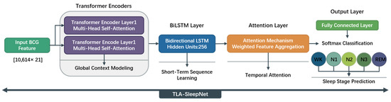
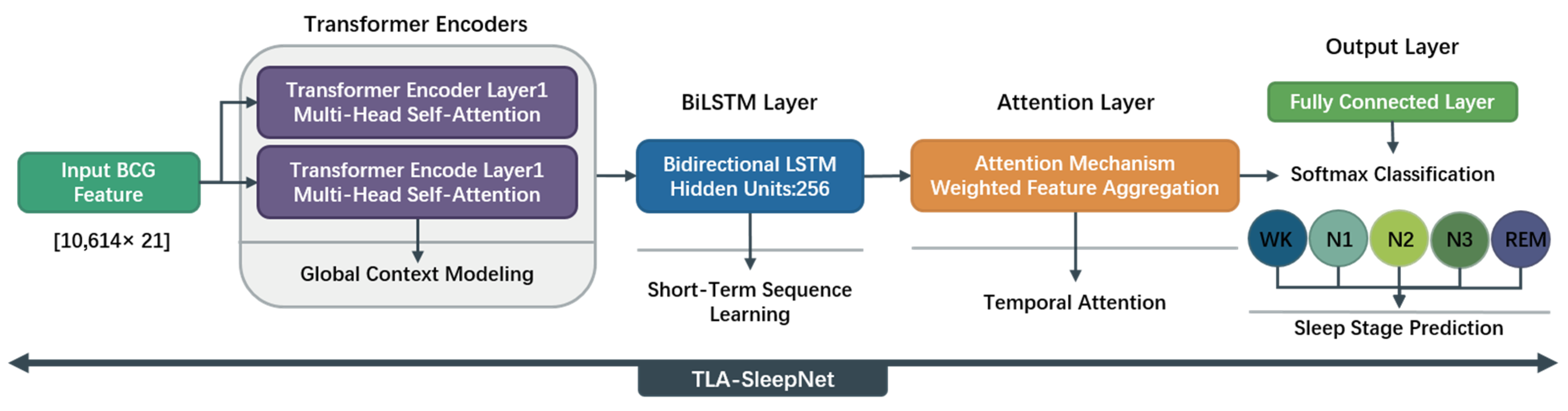
Normalization can be performed using z-score standardization, which scales each feature dimension to either the [0, 1] range or to have a mean of 0 and a variance of 1. The overall architecture of the proposed TLA-SleepNet model is illustrated in Figure 5.

Figure 5. TLA-SleepNet Model Architecture.

2.5.2. Positional Encoding

Since the Transformer model does not inherently encode temporal order and its self-attention mechanism is permutation-invariant over the input sequence, explicit positional information must be introduced to capture temporal dependencies. Therefore, this study incorporates continuous positional encoding (PE) based on sine and cosine functions into the input features, defined mathematically as follows:

$$H^{(0)}=\tilde{X}+PE$$

(13)

$PE\in R^{T\times d}$ represents the sinusoidal/cosine positional encoding, defined by the following formula:

$$P{E}_{(t,2i)}=\sin ({\displaystyle \frac{t}{\mathrm{10,00}{0}^{2i/d}}})$$

(14)

$$P{E}_{(t,2i+1)}=\cos ({\displaystyle \frac{t}{\mathrm{10,00}{0}^{2i/d}}})$$

(15)

This positional encoding provides each time step in the sequence with a unique positional representation, where t ∈ [1, T] and I ∈ [0, d/2–1]. By integrating the continuous positional encoding with the multi-scale HRV–RRV temporal features, the Transformer can effectively model the dynamic characteristics of physiological signals across different time scales without introducing additional recurrent structures, while providing temporally consistent and high-quality feature representations for the subsequent BiLSTM and Attention modules.

2.5.3. Transformer Encoder

The Transformer Encoder consists of 2 stacked encoder layers, each with d_model = 128, 8 attention heads, FFN dimension = 256, and dropout = 0.1. The Transformer Encoder models correlations between any time steps through self-attention, capturing global temporal dependencies in HRV–RRV feature sequences [31]:

$$\mathrm{A}\mathrm{t}\mathrm{t}\mathrm{e}\mathrm{n}\mathrm{t}\mathrm{i}\mathrm{o}\mathrm{n}(Q,K,V)=\mathrm{S}\mathrm{o}\mathrm{f}\mathrm{t}\mathrm{m}\mathrm{a}\mathrm{x}({\displaystyle \frac{Q{K}^T}{\sqrt{d_k}}})V$$

(16)

Multi-Head Attention (MHA) computes attention weights in parallel across multiple subspaces, enabling the model to capture multi-scale dynamic features of heart rate and respiratory signals from different representational perspectives:

$$MHA(H^{(l-1)})=Concat(hea{d}_1,\dots ,hea{d}_{\mathrm{h}})W_o$$

(17)

The combination of residual connections and Layer Normalization ensures the layer-wise propagation of feature information while effectively mitigating gradient vanishing and instability issues during the training of deep networks:

$$H^{(l)}=\mathrm{L}\mathrm{a}\mathrm{t}\mathrm{e}\mathrm{r}\mathrm{N}\mathrm{o}\mathrm{r}\mathrm{m}(H^{(l-1)}+\mathrm{M}\mathrm{H}\mathrm{A}(H^{(l-1)}))$$

(18)

After passing through L = 2 encoder layers, the global feature representation is obtained:

$$H_T=H^{(l)}\in R^{T\times d}$$

(19)

The model obtains high-level feature representations that integrate global temporal dependencies and multi-dimensional feature semantics, providing unified global contextual information for subsequent temporal modeling and attention-based discrimination.

2.5.4. BiLSTM Layer

To further capture local temporal dynamics, a BiLSTM layer is introduced with 256 hidden units and 1 stacked layer [32]:

$$\overleftarrow{h_t}=\mathrm{L}\mathrm{S}\mathrm{T}{\mathrm{M}}_{\mathrm{f}\mathrm{o}\mathrm{r}\mathrm{w}\mathrm{a}\mathrm{r}\mathrm{d}}(H_T)$$

(20)

$$\overleftarrow{h_t}=\mathrm{L}\mathrm{S}\mathrm{T}{\mathrm{M}}_{\mathrm{b}\mathrm{a}\mathrm{c}\mathrm{k}\mathrm{f}\mathrm{o}\mathrm{r}\mathrm{w}\mathrm{a}\mathrm{r}\mathrm{d}}(H_T)$$

(21)

$$h_t^{\mathrm{B}\mathrm{i}\mathrm{L}\mathrm{S}\mathrm{T}\mathrm{M}}=[\overleftarrow{h_t},\overleftarrow{h_t}]\in R^{2d_h}$$

(22)

where h_t denotes the dimensionality of the LSTM hidden units. The BiLSTM layer models temporal dependencies in both forward and backward directions, simultaneously capturing relationships between the current time step and its preceding and following contexts. This enables effective representation of short-term dynamic changes and local temporal structures. Built upon the global feature representations, this layer enhances the consistency and continuity of local temporal semantics, providing the subsequent attention module with more fine-grained and discriminative temporal feature representations.

2.5.5. Attention Layer

To emphasize the features of critical time periods for sleep stage determination, an attention mechanism is applied to weight the BiLSTM outputs:

$${\alpha }_t={\displaystyle \frac{exp(\mathrm{s}\mathrm{c}\mathrm{o}\mathrm{r}\mathrm{e}(h_t^{\mathrm{B}\mathrm{i}\mathrm{L}\mathrm{S}\mathrm{T}\mathrm{M}}))}{{\sum }_{t^{\prime }}{\alpha }_{t^{\prime }}{h}_{t\prime }^{\mathrm{B}\mathrm{I}\mathrm{L}\mathrm{S}\mathrm{T}\mathrm{M}}}}$$

(23)

$$H_{attn}={\sum }_{t=1}^T{\alpha }_t{h}_t^{\mathrm{B}\mathrm{i}\mathrm{L}\mathrm{S}\mathrm{T}\mathrm{M}}$$

(24)

where ${\alpha }_t$ represents normalized attention weights computed via softmax function. The weighted feature vector $H_{attn}\in R^{2d_{\mathrm{h}}}$ suppresses redundant temporal information while enhancing the discriminative representation of key time periods, thereby improving the model’s ability to distinguish between different sleep stages.

2.5.6. Fully Connected Output

Finally, the features are mapped to the sleep stage labels through a fully connected layer for prediction:

$${\widehat{y}}_{ϵ}={\displaystyle \frac{exp(w_C^T{H}_{attn}+b_{\mathrm{c}})}{{\sum }_{j=1}^{c}exp(w_C^T{H}_{attn}+b_j)}}$$

(25)

For the classification task, the output is passed through a Softmax function to obtain a probability distribution, where C is the number of sleep stage classes and W_c represents the learnable parameters.

In summary, the TLA-SleepNet model can be formulated as:

$${\widehat{y}}_{\mathrm{c}}=\mathrm{F}\mathrm{C}(\mathrm{A}\mathrm{t}\mathrm{t}\mathrm{e}\mathrm{n}\mathrm{t}\mathrm{i}\mathrm{o}\mathrm{n}(\mathrm{B}\mathrm{i}\mathrm{L}\mathrm{S}\mathrm{T}\mathrm{M}(\mathrm{T}\mathrm{r}\mathrm{a}\mathrm{n}\mathrm{s}\mathrm{f}\mathrm{o}\mathrm{r}\mathrm{m}\mathrm{r}(\overline{X}+PE))))$$

(26)

The Transformer captures global dependencies in the sequence, the BiLSTM captures local short-term dynamics, and the Attention mechanism reinforces key features. This design enables simultaneous modeling of short-term fluctuations and long-term trends in BCG signals, thereby improving the accuracy and robustness of sleep stage classification.

2.5.7. Training Configuration

The model is trained using the Adam optimizer with a learning rate of 0.005, batch size of 32, and a maximum of 500 iterations (epochs). A stepwise learning rate decay strategy is adopted with a decay factor of 0.5 every 100 iterations. Cross-entropy loss is used as the optimization objective.

To improve training stability and reduce the risk of overfitting, no early stopping strategy is applied in this study. Instead, the model relies on stepwise learning rate decay and dropout (0.1) as implicit regularization mechanisms. The training process shows stable convergence under the fixed-epoch setting.

3. Experiment

3.1. Data Availability

The BCG signals and corresponding sleep stage labels used in this study were provided by Bobo Technology (Suzhou) Co., Ltd. (Suzhou, China) and Sir Run Run Shaw Hospital, Zhejiang University School of Medicine. The dataset comprises 10 independent recordings, collected overnight using the MD-EA sleep monitor (Medical Device Registration No.: Su Xie Zhu Zhun 20232070772), and approved by the hospital ethics committee (Approval No.: Kexue 20190520-67). Sleep stages were scored in 30 s epochs by three licensed physicians, and epochs with inconsistent annotations were excluded. A total of 10,614 valid samples were obtained. Dataset parameters are summarized in Table 3.

Table 3. Sleep Sample Data Statistics.

Class Type	Data Value (%)
WK	1521 (14.33)
REM	2225 (20.96)
NREM (N1)	472 (04.45)
NREM (N2)	4433 (41.77)
NREM (N3)	1969 (18.49)
Total	10,614 (100)

3.2. Evaluation Metrics

To evaluate the model’s performance in the sleep staging task, this study employed Accuracy (ACC), Precision (PRE), Recall, F1-Score (F1), and Cohen’s Kappa (Kappa) as evaluation metrics:

$$\mathrm{A}\mathrm{c}\mathrm{c}\mathrm{u}\mathrm{r}\mathrm{a}\mathrm{c}\mathrm{y}={\displaystyle \frac{\mathrm{T}\mathrm{P}+\mathrm{T}\mathrm{N}}{\mathrm{T}\mathrm{P}+\mathrm{F}\mathrm{P}+\mathrm{T}\mathrm{N}+\mathrm{F}\mathrm{N}}}$$

(27)

$$\mathrm{P}\mathrm{r}\mathrm{e}\mathrm{c}\mathrm{i}\mathrm{s}\mathrm{i}\mathrm{o}\mathrm{n}={\displaystyle \frac{\mathrm{T}\mathrm{P}}{\mathrm{T}\mathrm{P}+\mathrm{F}\mathrm{P}}}$$

(28)

$$\mathrm{F}1={\displaystyle \frac{2\mathrm{T}\mathrm{P}}{2\mathrm{T}\mathrm{P}+\mathrm{F}\mathrm{P}+\mathrm{F}\mathrm{N}}}$$

(29)

$$\mathrm{R}\mathrm{e}\mathrm{c}\mathrm{a}\mathrm{l}\mathrm{l}={\displaystyle \frac{\mathrm{T}\mathrm{P}}{\mathrm{T}\mathrm{P}+\mathrm{F}\mathrm{N}}}$$

(30)

$$\mathrm{Kappa}={\displaystyle \frac{{\mathrm{p}}_0-{\mathrm{p}}_{\mathrm{e}}}{1-{\mathrm{p}}_{\mathrm{e}}}}$$

(31)

$${\mathrm{P}}_0={\displaystyle \frac{\mathrm{T}\mathrm{P}+\mathrm{T}\mathrm{N}}{\mathrm{T}\mathrm{P}+\mathrm{F}\mathrm{P}+\mathrm{T}\mathrm{N}+\mathrm{F}\mathrm{N}}}$$

(32)

$${\mathrm{P}}_{\mathrm{e}}={\displaystyle \frac{(\mathrm{T}\mathrm{P}+\mathrm{F}\mathrm{N})(\mathrm{T}\mathrm{P}+\mathrm{F}\mathrm{P})+(\mathrm{T}\mathrm{N}+\mathrm{F}\mathrm{P})(\mathrm{T}\mathrm{N}+\mathrm{F}\mathrm{N})}{(\mathrm{T}\mathrm{P}+\mathrm{F}\mathrm{P}+\mathrm{T}\mathrm{N}+\mathrm{F}\mathrm{N}{)}^2}}$$

(33)

In the equations, True Positive (TP) denotes the number of samples correctly classified as class i. False Negative (FN) represents the number of samples belonging to class i that are incorrectly classified as other classes. False Positive (FP) refers to the number of samples from other classes that are incorrectly classified as class i. True Negative (TN) denotes the number of samples correctly identified as not belonging to class i.

Since the real-world sleep dataset exhibits class imbalance, weighted evaluation metrics are adopted to comprehensively and fairly reflect the overall model performance. Specifically, weighted Precision (PRE) and weighted F1-score are employed, where the weight of each class is determined by the ratio between the number of samples in the current class and the total number of samples.

4. Experimental Results

4.1. Feature Selection

Based on the RRi and BBi sequences, this study comprehensively extracts multi-dimensional HRV and RRV features, including time-domain, frequency-domain, nonlinear-domain, complexity indices, and Poincaré plot geometry features, which are summarized in Table 4. By performing window-based analysis of respiratory signals at different temporal scales, physiological information is extracted and mapped to corresponding sleep stages.

Table 4. HRV and RRV Feature Summary.

Number	Feature Name
18	Time-Domain Features
6	Mean, Max, and Min for the JJ sequence and BB sequence.
10	RMSSD, SDNN, SDSD, CVNN, and CVSD for the JJ sequence and BB sequence.
2	PNN20 and PNN50 for the JJ sequence.
24	Frequency-Domain Features
8	LF, HF, MF, and TLF for the JJ sequence and BB sequence.
8	LFf, HFf, MFf, and TLFf for the JJ sequence and BB sequence.
8	LFn, HFn, MFn, and TLFn for the JJ sequence and BB sequence.
8	Poincaré Plot Geometric Features
8	SD1, SD2, SD1SD2, and S for the JJ sequence and BB sequence.
14	Heart Rate Fragmentation Index
14	GI, C1d, C1a, SD1d, SD1a, C2d, C2a, SD2d, SD2a, SD2I, Cd, Ca, SDNNd, and SDNNa for the JJ sequence.
2	Complexity Index
2	SampEn for the JJ sequence and BB sequence.

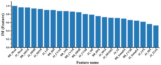
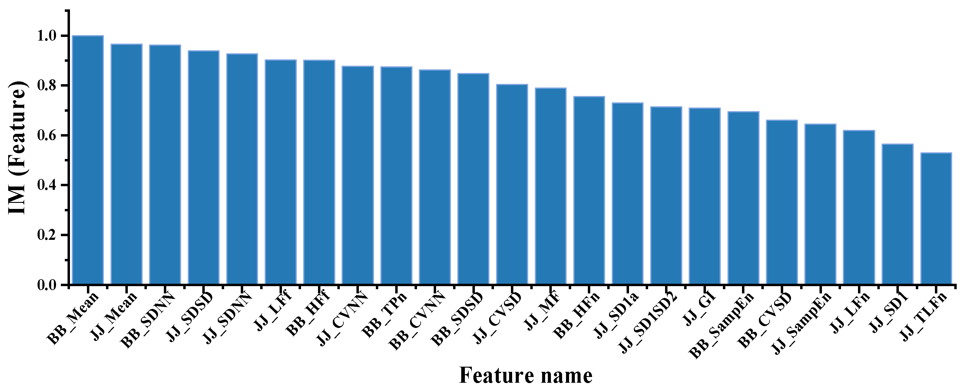
A total of 66 HRV and RRV features are obtained, and MI is employed for feature selection. To enhance the stability of the selection process, the MI values are normalized, and features with values lower than the average threshold of 0.62 are removed. In the subsequent feature dimensionality reduction experiments, the TOP-23 most representative features are selected. The distribution of the normalized MI values is illustrated in Figure 6.

Figure 6. Feature Importance Ranking.

4.2. Model Parameter Evaluation

In this study, the proposed TLA-SleepNet model was used to perform sleep stage prediction based on single-channel BCG signals. The dataset consists of 10,614 samples from 10 subjects, with each sample represented by a 23-dimensional feature vector and categorized into five sleep stages.

To clarify the validation protocol, five-fold cross-validation is performed at the epoch level, where approximately 80% of the data are used for training and 20% for testing in each fold. Since the split is conducted at the epoch level, samples from all subjects may appear in both the training and test sets. Due to the small number of subjects, epoch-level cross-validation was adopted to ensure sufficient training samples and stable model optimization, with each segment corresponding to a different temporal context.

To ensure the reproducibility and generalization of the results, all experiments are conducted under a unified model architecture and consistent parameter settings.

The experiments were performed on a local workstation equipped with an Intel Core i7-8750H CPU @ 2.20 GHz. Based on the TOP-23 HRV and RRV features, the average training time under five-fold cross-validation is approximately 1.2–1.4 h per fold, indicating a reasonable computational cost and suitability for practical offline training.

This study performs ablation experiments based on the TOP-23 feature set to evaluate the contribution of each module to overall performance. BiLSTM, BiLSTM-Attention, and Transformer-BiLSTM are used as comparison models to analyze the performance gains from the attention mechanism and Transformer encoder. The results are summarized in Table 5.

Table 5. Comparison of Ablation Study Results.

Model	ACC (%)	PRE (%)	Kappa (%)
BiLSTM	80.95	82.80	73.15
BiLSTM-Attention	82.22	86.14	75.11
Transformer-BiLSTM	84.04	90.12	79.23
TLA-SleepNet	87.19	92.44	81.94

To evaluate the effectiveness and robustness of TLA-SleepNet, we conduct comparative experiments under two feature configurations, reporting confusion matrices, stage-wise metrics (Recall, Precision, and F1-score), and overall performance indicators (Accuracy, F1-score, and Kappa). These experiments aim to assess classification performance across different sleep stages, especially for confusable stages (e.g., N1–N2 and REM–W), and to analyze the impact of different feature representations on model performance, thereby validating the stability and contribution of feature design to sleep staging. The results are summarized in Table 6 and Table 7.

Table 6. Sleep Staging Performance of TLA-SleepNet Based on HRV and RRV Feature Sets.

	Confusion Matrix (%)					Evaluation by Stage (%)			Overall Model Evaluation (%)
	N1	N2	N3	REM	W	Recall	PRE	F1	ACC:	86.58
N1	7.20	59.32	4.24	6.36	22.88	7.20	24.64	11.15	PRE:	91.26
N2	1.35	92.13	4.06	0.90	1.56	92.13	81.56	86.53	F1:	81.08
N3	0.51	10.16	85.63	1.02	2.69	85.63	93.68	89.44	Kappa:	88.36
REM	0.67	1.80	0.90	92.31	4.31	92.31	88.03	90.11
W	1.31	2.63	0.66	7.50	87.90	87.90	82.50	85.06

Table 7. Sleep Staging Performance of TLA-SleepNet on the Top-23 Feature Sets.

	Confusion Matrix (%)					Evaluation by Stage (%)			Overall Model Evaluation (%)
	N1	N2	N3	REM	W	Recall	PRE	F1	ACC:	87.19
N1	11.23	56.80	5.20	6.10	20.67	11.23	26.45	15.78	PRE:	92.44
N2	1.10	93.14	3.60	0.80	1.36	93.14	82.30	87.36	F1:	81.94
N3	0.45	11.30	85.33	1.92	1.92	85.33	94.10	89.37	Kappa:	88.74
REM	0.60	2.10	0.90	92.54	3.86	92.54	89.20	90.84
W	1.20	2.80	0.70	7.33	87.97	87.97	83.05	85.44

To further evaluate the effectiveness and superiority of the proposed model, TLA-SleepNet is compared with representative baseline methods, including traditional machine learning models, ensemble-based boosting methods, and deep learning models. Specifically, the compared methods include Random Forest (RF), GBDT, Light Gradient Boosting Machine (LightGBM), ELM, SVM, ResNet, Temporal Convolutional Network (TCN), and Recurrent Neural Network (RNN). All models are evaluated under identical feature representations, dataset splitting strategy, and consistent cross-validation protocol to ensure a fair comparison. The classification results are presented in Table 5, while Table 6 reports the results after feature selection using the TOP-23 subset, where all baseline models and the proposed method are assessed under a unified experimental setting using the same evaluation metrics (ACC, PRE, F1-score, and Kappa) for systematic comparison.

The classification results are presented in Table 8, while Table 9 reports results after feature selection using the TOP-23 subset, where all baseline models and the proposed method are evaluated under a unified experimental protocol using the same metrics (ACC, PRE, F1-score, and Kappa) for systematic comparison.

Table 8. Sleep Staging Results Based on HRV and RRV Feature Matrix.

Model	Recall (%)					ACC (%)	PRE (%)	Kappa (%)	F1 (%)
	N1	N2	N3	REM	WK
RF	7.42	88.50	74.33	81.08	73.96	78.63	84.97	69.65	79.29
GBDT	8.26	88.47	88.79	82.11	73.31	81.46	64.36	74.12	74.63
LightGBM	7.41	93.23	79.13	87.13	81.98	82.91	93.12	77.67	85.97
XgBoost	7.85	85.19	74.97	86.35	84.19	81.19	83.21	71.03	80.51
ELM	4.24	75.73	56.39	66.11	68.11	65.87	63.15	51.73	59.58
SVM	0.00	87.05	43.25	61.80	51.22	64.65	76.08	47.90	NaN
ResNet	4.24	90.48	72.24	80.36	69.43	78.13	86.52	68.60	78.73
CNN-LSTM	10.14	87.23	77.31	85.19	84.11	81.05	82.18	73.24	80.15
TCN	7.14	84.21	74.90	80.94	79.88	78.01	80.41	68.61	77.23
RNN	8.05	90.15	81.09	85.87	81.07	81.91	87.95	76.01	83.91
Ours	7.20	92.13	85.63	92.31	87.90	86.58	91.26	81.08	88.36

Table 9. Sleep Staging Results Based on TOP-23 Weighted Feature Matrix.

Model	Recall (%)					ACC (%)	PRE (%)	Kappa (%)	F1 (%)
	N1	N2	N3	REM	WK
RF	5.08	87.05	87.77	78.47	71.73	79.55	61.60	71.44	72.39
GBDT	10.34	90.28	91.29	87.51	81.53	85.52	74.51	79.85	82.05
LightGBM	10.58	94.21	81.29	89.39	81.78	85.64	93.45	79.78	87.41
XgBoost	13.94	84.55	84.72	84.94	81.00	81.46	81.14	74.29	81.26
ELM	13.14	83.80	77.79	80.36	80.80	78.40	78.55	69.69	78.17
SVM	0.64	90.86	62.40	73.48	65.09	74.25	89.68	62.57	73.60
ResNet	5.72	93.37	80.08	88.90	83.30	84.63	92.74	78.09	85.95
CNN-LSTM	13.74	87.64	80.93	85.48	83.67	82.12	86.14	75.56	83.12
TCN	11.25	85.90	77.49	85.75	82.48	81.51	83.42	73.26	80.42
RNN	9.76	87.55	84.14	89.04	84.12	83.95	85.83	76.89	84.90
Ours	11.23	93.14	85.33	92.54	87.97	87.19	92.44	81.94	88.74

5. Discussion

The experimental results (Table 5, Table 6, Table 7, Table 8 and Table 9) demonstrate that TLA-SleepNet achieves a stable and superior performance across different feature configurations, with consistent improvements in overall accuracy and key stage recognition.

Ablation results (Table 5) confirm the effectiveness of each module. TLA-SleepNet achieves 87.19% ACC, outperforming BiLSTM (80.95%) by 6.24%, indicating that recurrent structures alone are insufficient for modeling complex sleep transitions. Incorporating attention improves ACC to 82.22%, enhancing discrimination of ambiguous stages (N1/N2), while the Transformer further increases ACC to 84.04% by strengthening long-range dependency modeling. The final model reaches a Kappa of 81.94% (~8% higher than BiLSTM), demonstrating reduced class confusion and highlighting the complementary roles of local and global temporal modeling.

From the confusion matrices (Table 6 and Table 7), TLA-SleepNet achieves an ACC/Kappa of 86.58%/88.36% under original features, improving to 87.19%/88.74% after TOP-23 feature selection. A high performance is maintained in major stages, with Recall exceeding 92% for N2 and REM, ~85% for N3, and ~88% for W. For the challenging N1 stage, Recall improves from 7.20% to 11.23% and F1-score from 11.15% to 15.78%, while misclassification to N2 decreases (59.32% to 56.80%), indicating improved discrimination of transitional stages.

Comparative results (Table 8 and Table 9) further validate these findings. After further introducing the MI algorithm for feature selection, performance improves across all models, which confirms that feature redundancy reduction benefits both traditional machine learning and deep learning methods under the same evaluation setting. Under HRV and RRV features (Table 8), the best baseline (LightGBM) achieves 82.91% ACC, while TLA-SleepNet reaches 86.58% with a higher Kappa (88.36%). Deep learning baselines such as RNN (81.91%) and TCN (78.01%) remain inferior, reflecting weaker temporal modeling capacity. However, their F1-score and Kappa coefficient remain significantly lower than those of the proposed method, indicating limited capability in capturing long-range temporal dependencies compared to the hybrid architecture.

With the TOP-23 subset (Table 9), performance improves across models; however, TLA-SleepNet maintains the best results, achieving 87.19% ACC and 88.74% Kappa, outperforming LightGBM (85.64%) and RNN (83.95%). Importantly, it achieves a superior performance on N1 (Recall: 11.23%), which is significantly higher than RF (5.08%) and SVM (0.64%), demonstrating enhanced capability for minority class learning.

The low Recall of N1 (<15%) is mainly due to class imbalance and intrinsic ambiguity. N1 samples are limited and highly similar to adjacent stages, especially N2, resulting in frequent misclassification. As a transitional stage, N1 exhibits weak and unstable physiological patterns, and BCG-derived features provide limited discriminative information, making robust classification challenging. To improve performance on imbalanced stages such as N1, strategies such as cost-sensitive loss, class re-weighting or focal loss, and temporal smoothing could be adopted, and will be explored in future work.

From a deployment perspective, although TLA-SleepNet adopts a relatively complex architecture, the training process is performed offline. Once trained, the model enables efficient inference, making it suitable for deployment in practical home-monitoring systems with limited computational resources.

Overall, TLA-SleepNet consistently achieves a superior accuracy and robustness, maintaining a high performance on dominant stages while improving recognition of ambiguous transitions, thereby demonstrating strong generalization for single-channel BCG-based sleep staging.

In advanced studies, as shown in Table 10, EEG-based sleep staging methods can achieve 85.4% accuracy in five-stage classification, while EOG- and PPG-based approaches achieve higher accuracies of 91.72% and 93.6% in four-stage settings, respectively. However, these methods rely on contact-based sensors such as electrodes or wearable devices, which limit their applicability in long-term and home-based monitoring scenarios.

Table 10. Comparison with Advanced Studies.

Author	Signal	Model	Stage	ACC (%)
Chen Lingling et al. [3]	EEG	RSNSleepNet	5	85.4
Du-Yan et al. [4]	EOG	CNN	4	91.72
Ahsan Habib et al. [5]	PPG	CNN	4	93.6
Wang W. B. et al. [6]	ECG	GBDT	5	77.00
Rahman et al. [7]	CW radar	LSTM	2	80.2
Yu B. et al. [8]	Wi-Fi	CNN-LSTM	4	89.6
Li Siheng et al. [9]	UWB	LSTM	4	81.1
Jing Jianmeng et al. [14]	BCG	L-ChainCRF	5	61.80
Luo Yi et al. [15]	BCG	SVM	4	72.50
Yi R. et al. [16]	BCG	SVM	3	74.00
Ahmed N. et al. [17]	BCG	1D-CNN	2	94.16
Ours	BCG	TLA-SleepNet	5	87.19

Non-contact sensing modalities, including CW radar, Wi-Fi, and UWB, have also been explored for sleep staging, achieving accuracies of 80.2% (two-stage), 89.6% (four-stage), and 81.1% (four-stage), respectively. Nevertheless, these approaches are generally limited in staging granularity and are sensitive to environmental conditions.

It is important to note that the methods summarized in Table 10 differ in multiple aspects, including sensing modality (e.g., EEG, EOG, PPG, radar, Wi-Fi, and BCG), number of sleep stages (ranging from binary to five-stage classification), and evaluation protocols. These factors inevitably influence the reported performance, and the comparisons presented here are intended to provide a broad overview of existing approaches rather than strict one-to-one quantitative equivalence.

For BCG-based studies, existing methods still face challenges in fine-grained sleep staging. Traditional approaches such as L-ChainCRF and SVM achieve relatively limited performance in five-stage and four-stage tasks, respectively. Although deep learning methods can achieve a high accuracy in binary classification (e.g., 94.16% for 2-stage), they are not directly comparable in fine-grained sleep structure analysis.

In this context, the main contribution of this study is not solely reflected in accuracy improvement, but in enabling five-stage sleep staging using single-channel non-contact BCG signals, which remains a challenging and underexplored problem. The proposed TLA-SleepNet achieves 87.19% accuracy under this setting, demonstrating the feasibility of fine-grained sleep staging using BCG signals in practical non-contact monitoring scenarios.

Further analysis indicates that the proposed TLA-SleepNet modeling framework consistently outperforms the comparison models under different feature conditions. By jointly modeling global temporal dependencies, local dynamic features, and key feature weights, the model achieves efficient feature representation for long-term BCG sequences, thereby significantly improving fine-grained sleep staging performance while maintaining the advantages of non-contact signal acquisition.

In addition, it should be noted that the dataset contains recordings from 10 subjects, which may limit the inter-subject variability. To address this, the adopted epoch-level cross-validation strategy enables more efficient data utilization by incorporating samples from all subjects across different folds, allowing the model to learn more representative and generalized feature patterns. While this strategy improves data utilization, further evaluation under subject-independent protocols (e.g., LOSO) would be beneficial to assess generalization across unseen individuals. This will be considered in future work with larger-scale datasets.

6. Conclusions

This study addresses common challenges in BCG-based sleep staging, including low signal-to-noise ratio, complex temporal dependencies, and redundancy in high-dimensional features. A non-contact automatic sleep staging method based on HRV and RRV feature fusion is proposed, and a TLA-SleepNet model is constructed to effectively model multi-scale physiological information in long-term BCG signals.

At the signal processing level, the raw BCG signals are separated and reconstructed using low-pass filtering and discrete wavelet transform, allowing the extraction of cardiac-related JJi sequences and respiration-related BBi sequences. This process suppresses the influence of body motion artifacts and environmental noise, providing stable and reliable inputs for subsequent feature extraction and modeling.

Subsequently, a multi-dimensional feature set is constructed based on HRV and RRV characteristics. To address redundancy and noise in high-dimensional features, the MI algorithm is employed to select feature subsets that are highly correlated with sleep stages. This strategy effectively reduces feature dimensionality while improving training efficiency and model generalization stability.

Based on the optimized feature set, TLA-SleepNet performs temporal modeling of the fused multi-scale features, enabling comprehensive characterization of long-term trends and key temporal patterns in BCG signals across different sleep stages.

Experimental results show that the proposed method achieves a classification accuracy of 87.19% on a non-independent test dataset, significantly outperforming the comparison models. The model also demonstrates stable staging performance across different individuals and data distributions, confirming its strong adaptability and robustness for long-term BCG signal analysis.

Compared with traditional approaches that rely on contact-based physiological signals such as EEG and EOG, the proposed method significantly reduces the invasiveness of signal acquisition while maintaining competitive staging performance, making it promising for long-term home-based sleep monitoring applications.

References

- Berry, R.B.; Brooks, R.; Gamaldo, C.; Harding, S.M.; Lloyd, R.M.; Quan, S.F.; Troester, M.T.; Vaughn, B.V. AASM scoring manual updates for 2017 (version 2.4). J. Clin. Sleep Med. 2017, 13, 665–666. [Google Scholar] [CrossRef] [Scilit]
- Kosmadopoulos, A.; Sargent, C.; Darwent, D.; Zhou, X.; Roach, G.D. Alternatives to polysomnography (PSG): A validation of wrist actigraphy and a partial-PSG system. Behav. Res. Methods 2014, 46, 1032–1041. [Google Scholar] [CrossRef] [Scilit]
- Chen, L.; Bi, X. Sleep EEG staging based on residual shrinkage network. J. Instrum. 2022, 43, 148–155. [Google Scholar]
- Geng, D.-Y.; Wang, J.-X.; Wang, Y.; Liu, X.-Y. Convolutional neural network is a good technique for sleep staging based on HRV: A comparative analysis. Neurosci. Lett. 2022, 779, 136550. [Google Scholar] [CrossRef] [Scilit] [PubMed]
- Habib, A.; Motin, M.A.; Penzel, T.; Palaniswami, M.; Yearwood, J.; Karmakar, C. Performance of a Convolutional Neural Network Derived from PPG Signal in Classifying Sleep Stages. IEEE Trans. Biomed. Eng. 2022, 70, 1717–1728. [Google Scholar] [CrossRef] [Scilit] [PubMed]
- Wang, W.B.; Qin, D.; Fang, Y.; Zhou, C.; Zheng, Y.K. Automatic multi-class sleep staging method based on novel hybrid features. J. Electr. Eng. Technol. 2023, 19, 709–722. [Google Scholar] [CrossRef] [Scilit]
- Rahman, T.; Adams, A.T.; Ravichandran, R.V.; Zhang, M.; Patel, S.N.; Kientz, J.A.; Choudhury, T. DoppleSleep: A contactless unobtrusive sleep sensing system using short-range doppler radar. In UbiComp ’15, Proceedings of the 2015 ACM International Joint Conference on Pervasive and Ubiquitous Computing, Osaka, Japan, 7–11 September 2015; ACM: New York, NY, USA, 2015; pp. 39–50. [Google Scholar]
- Yu, B.; Wang, Y.; Niu, K.; Zeng, Y.; Gu, T.; Wang, L.; Guan, C.; Zhang, D. WiFi-sleep: Sleep stage monitoring using commodity Wi-Fi devices. IEEE Internet Things J. 2021, 8, 13900–13913. [Google Scholar] [CrossRef] [Scilit]
- Li, S.; Jin, B.; Zhang, F.; Wang, Z.; Ma, J.; Su, C.; Ren, X.; Liu, H. Non-contact sleep monitoring based on multi-task attention network. Comput. Res. Dev. 2024, 61, 2739–2753. [Google Scholar]
- Pullano, S.A.; Critello, D.C.; Fiorillo, A.S. Triboelectric-induced Pseudo-ICG for cardiovascular risk assessment on flexible electronics. Nano Energy 2020, 67, 104278. [Google Scholar] [CrossRef] [Scilit]
- Laganà, F. Design and Simulation-Based Validation of an Embedded Acquisition Architecture for In Situ PCB Integrity Monitoring in Biomedical Devices. Electronics 2026, 15, 833. [Google Scholar] [CrossRef] [Scilit]
- Shin, J.H.; Choi, B.H.; Lim, Y.G.; Jeong, D.U.; Park, K.S. Automatic ballistocardiogram (BCG) beat detection using a template matching approach. In Proceedings of the 2008 30th Annual International Conference of the IEEE Engineering in Medicine and Biology Society, Vancouver, BC, Canada, 20–24 August 2008; pp. 1144–1146. [Google Scholar]
- Kumar, P.; Das, A.K.; Halder, S. Respiration rate variability analysis under different body postures. In Proceedings of the 2020 IEEE-HYDCON, Hyderabad, India, 11–12 September 2020; pp. 1–4. [Google Scholar]
- Jing, J. Research on Automatic Sleep Staging Method Based on BCG Signals. Master’s Thesis, Chongqing University, Chongqing, China, 2022. [Google Scholar]
- Luo, Y.; Wang, D.; Zhao, Z.; Wang, J.; Wu, Y. A P(VDF-TrFE)/PZT piezoelectric sensor fabricated by high-voltage electrospinning and its application in sleep monitoring. J. Sens. Technol. 2024, 37, 345–352. [Google Scholar]
- Yi, R.; Enayati, M.; Keller, J.M.; Popescu, M.; Skubic, M. Non-invasive in-home sleep stage classification using a ballistocardiography bed sensor. In Proceedings of the 2019 IEEE EMBS International Conference on Biomedical & Health Informatic, Chicago, IL, USA, 19–22 May 2019; pp. 1–4. [Google Scholar]
- Ahmed, N.; Srivyshnav, K.S.; Chokalingam, K.; Rawooth, M.; Kumar, G.; Parchani, G.; Saran, V. Classification of Sleep-Wake State in Ballistocardiogram system based on Deep Learning. In Proceedings of the 2022 44th Annual International Conference of the IEEE Engineering in Medicine & Biology Society, Glasgow, UK, 11–15 July 2022; pp. 1944–1947. [Google Scholar]
- Hussin, S.F.; Birasamy, G.; Hamid, Z. Design of butterworth band-pass filter. Politek. Kolej Komuniti J. Eng. Technol. 2016, 1, 32–46. [Google Scholar]
- Tschannen, M.; Djolonga, J.; Rubenstein, P.K.; Gelly, S.; Lucic, M. On mutual information maximization for representation learning. arXiv 2019, arXiv:1907.13625. [Google Scholar]
- Sadek, I.; Biswas, J.; Abdulrazak, B. Ballistocardiogram signal processing: A review. Health Inf. Sci. Syst. 2019, 7, 10. [Google Scholar] [CrossRef] [Scilit]
- Schranz, C.; Halmich, C.; Mayr, S.; Heib, D.P.J. Surrogate modelling of heartbeat events for improved J-peak detection in BCG using deep learning. Front. Netw. Physiol. 2024, 4, 1425871. [Google Scholar] [CrossRef] [Scilit]
- Casanella, R.; Gomez-Clapers, J.; Pallas-Areny, R. On time interval measurements using BCG. In Proceedings of the 2012 Annual International Conference of the IEEE Engineering in Medicine and Biology Society, San Diego, CA, USA, 28 August–1 September 2012; pp. 5034–5037. [Google Scholar]
- Aggarwal, Y.; Das, J.; Mazumder, P.M.; Kumar, R.; Sinha, R.K. Heart rate variability time domain features in automated prediction of diabetes in rat. Phys. Eng. Sci. Med. 2021, 44, 45–52. [Google Scholar] [CrossRef] [Scilit]
- Youngworth, R.N.; Gallagher, B.B.; Stamper, B.L. An overview of power spectral density (PSD) calculations. Opt. Manuf. Test. VI 2005, 5869, 206–216. [Google Scholar]
- Lubis, M.Z.; Si, M. Signal processing for power spectral density (PSD). In Signal Processing for Marine Acoustic and Dolphin Using Matlab; Lambert Academic Publishing: London, UK, 2016. [Google Scholar]
- Kamen, P.W.; Krum, H.; Tonkin, A.M. Poincare plot of heart rate variability allows quantitative display of parasympathetic nervous activity in humans. Clin. Sci. 1996, 91, 201–208. [Google Scholar] [CrossRef] [Scilit]
- International Brotherhood of Electrical Workers (IBEW); National Electrical Contractors Association (NECA). Standard for Installing and Maintaining Electrical Power Systems (HRA). 1995. Available online: https://www.scibew-neca.org/html/sbc-hra-2018.pdf (accessed on 15 April 2026).
- Karmakar, C.; Khandoker, A.; Palaniswami, M. Investigating the changes in heart rate asymmetry (HRA) with perturbation of parasympathetic nervous system. Australas. Phys. Eng. Sci. Med. 2012, 35, 465–474. [Google Scholar] [CrossRef] [Scilit]
- Bhavsar, R.; Helian, N.; Sun, Y.; Davey, N.; Steffert, T.; Mayor, D. Efficient methods for calculating sample entropy in time series data analysis. Procedia Comput. Sci. 2018, 145, 97–104. [Google Scholar] [CrossRef] [Scilit]
- Walters-Williams, J.; Li, Y. Estimation of mutual information: A survey. In International Conference on Rough Sets and Knowledge Technology; Springer: Berlin/Heidelberg, Germany, 2009; pp. 389–396. [Google Scholar]
- Chen, H.; Jiang, D.; Sahli, H. Transformer encoder with multi-modal multi-head attention for continuous affect recognition. IEEE Trans. Multimed. 2020, 23, 4171–4183. [Google Scholar] [CrossRef] [Scilit]
- Lee, M.; Kang, H.; Yu, S.-H.; Cho, H.; Oh, J.; van der Lande, G.; Gosseries, O.; Jeong, J.-H. Automatic sleep stage classification using nasal pressure decoding based on a multi-kernel convolutional bilstm network. IEEE Trans. Neural Syst. Rehabil. Eng. 2024, 32, 2533–2544. [Google Scholar] [CrossRef] [Scilit]
Disclaimer/Publisher’s Note: The statements, opinions and data contained in all publications are solely those of the individual author(s) and contributor(s) and not of MDPI and/or the editor(s). MDPI and/or the editor(s) disclaim responsibility for any injury to people or property resulting from any ideas, methods, instructions or products referred to in the content. |
© 2026 by the authors. Licensee MDPI, Basel, Switzerland. This article is an open access article distributed under the terms and conditions of the Creative Commons Attribution (CC BY) license.