Denoising Auto-Encoder-Enhanced Deep Non-Negative Matrix Factorization Clustering Model

Abstract

Non-negative matrix factorization directly decomposes data features into a base matrix and community matrix, which are easily affected by noise. Multi-view datasets have multiple feature matrices, each with a different angle. The data features need to be re-synthesized rather than simply concatenated or added. Based on the advantages and disadvantages of multi-view clustering and non-negative matrix factorization, we attempt to transplant the method of analyzing abstract connected graphs, analogize the similarity between edges and samples in the graph, and propose a deep non-negative matrix factorization model for clustering by constructing a similarity matrix and decomposing it. At the same time, in order to reduce the interference of noise, we introduce a denoising auto-encoder and non-negative matrix factorization in series, and research the reconstruction features, ultimately forming a model structure framework of “denoising auto-encoder, non-negative matrix factorization, clustering”. Through experiments, the denoising auto-encoder-enhanced non-negative matrix factorization achieved good results on five datasets. It achieved an accuracy of 87 percenton the BBC Sport dataset and 61 percent on Wiki-fea, which increased by two percentage points. The clustering results demonstrate that the model can effectively alleviate the impact of noise and provide new ideas for how to integrate multi-view features.

1. Introduction

The data in the real world is diverse, and the same set of samples can also be depicted from multiple perspectives. In the 3Sources dataset, the same news event can be reported by the BBC, The Guardian, or Reuters. Three different sources of reports constitute three views of the same data sample. Correspondingly, multi-view clustering has also become a research hotspot in recent years [1,2,3,4]. Scholars have proposed various methods, including spectral clustering from spectral analysis [5,6,7,8], subspace clustering focusing on low rank subspace analysis [9,10,11,12], and non-negative matrix factorization [13,14]. The spectral clustering method converts data into a graph and examines the connections between nodes, and uses graph constraints and graph regularization methods to extract meaningful clustering structures. However, graph constraints are largely based on so-called “inspiration” or the characteristics of the dataset itself, making them difficult to generalize. Similarly, how to reasonably embed prior information into constraints has become a major challenge. Subspace clustering methods focus on the low rank subspaces shared by various feature datasets, and obtain meaningful clustering results by extracting consensus and combining possible regularization constraints and graph constraints. However, subspace clustering methods are prone to noise interference, and the subspaces shared by data from different views are not exactly the same, which always limits further performance improvement. In the end, non-negative matrix factorization gradually demonstrated a performance and advantages beyond the former, becoming a popular method in recent years.

At the same time, in order to solve problems such as noise pollution, data reconstruction, and image restoration, auto-encoder methods have been proposed and quickly widely adopted. The core idea is to obtain the low rank hidden space representation of data through layer by layer encoding, compress the originally large and complex data through encoding, and then restore the data through decoding. With the widespread application of auto-encoders, the idea of auto-encoders has also entered other types of machine learning methods, combining the structure of auto-encoders with the function of non-negative matrix factorization to form a class auto-encoder non-negative matrix factorization algorithm, which achieves results beyond the original graph and spectral methods and has become a research hotspot.

In the non-negative matrix factorization method, the combination of non-negative matrix factorization and auto-encoder theory forms a deep non-negative matrix factorization theoretical framework for auto-encoders [15]. This method converts the original feature matrix into the product of a base matrix and feature matrices at different levels, revealing the multi-level internal features of datasets. This advantage has made it a popular method at present. At present, there are already a large number of non-negative matrix factorization models inspired by auto-encoder structures and graph constraints, including models that integrate dual graph constraints, models that integrate non-negative semi-positive definite matrix constraints, and models that use Laplace constraints. However, these models have achieved good results on their respective datasets. However, once these models are extended to other datasets, the constraints on which they rely will become ineffective, and their clustering results will significantly decrease. At the same time, the impact of noise remains prominent.

In summary, there are still two challenges in multi-view clustering: firstly, the data formats of each view may be different, and all contain meaningless noises, which will corrupt data and mislead researchers; secondly, each view essentially extracts data features from different perspectives, and views need to be re-synthesized and regulated [15], while most constraints are based on graphs and are closely related to the dataset, making them difficult to generalize. In order to comprehensively address these two main challenges, this paper combines graph-based denoising auto-encoders with deep non-negative matrix factorization models [16], and makes corresponding improvements for multi-view clustering, proposing a new denoising auto-encoder-enhanced deep non-negative matrix factorization clustering model. Our algorithm has several contributions:

1.

A new framework based on NMF for multi-view data auto-encoder and integrated similarity constraints has been proposed. This framework not only provides a more universal constraint scheme, but also reduces the impact of noise and improves the robustness of the model.

2.

Denoising auto-encoders with ordinary auto-encoders was compared and studied, and the effectiveness of denoising auto-encoders verified.

3.

We conducted experiments on five publicly available datasets. The experimental results demonstrate the effectiveness and robustness of the proposed algorithm.

The following text will provide a detailed presentation of the basic model, improvements and innovations, experimental results, and prospects for conclusions.

2. Background Models

2.1. Deep Non-Negative Matrix Factorization Model

The deep non-negative matrix factorization model was proposed by the researchers Chen Chuan and Zhang Zibin from Sun Yat-sen University [17]. It is dedicated to the machine learning task of extracting communities from abstract graphs for clustering. The traditional method is to directly decompose, or to use various auxiliary algorithms such as auto-encoders [18,19] for abstract graphs combined with non-negative matrix factorization [7,16]. However, traditional auto-encoder methods still have drawbacks, such as excessive complexity. In order to address the shortcomings of traditional single-layer non-negative matrix factorization, researchers have attempted to introduce a multi-layer structure similar to auto-encoders on the basis of non-negative matrix factorization [20]. Traditional non-negative matrix factorization is as follows:

$$\begin{array}{c}\begin{array}{c}\underset{\begin{array}{c}\mathit{U},\mathit{V}\end{array}}{\min }\left|\right|\mathit{X}-{\displaystyle {\mathit{U}\mathit{V}\left|\right|}_F^2},s.t.\mathit{U},\mathit{V}\ge O.\hfill \end{array}\hfill \end{array}$$

(1)

Here, U is called the mapping and community similarity matrix, representing how the basic elements in the dataset are combined, while V is called the community member matrix, representing which basic elements are included in the dataset. The character ${\left|\right|·\left|\right|}_F$ stands for Frobenius norm and $\mathit{min}$ means minimizing. The optimal solution is obtained when the Frobenius norm of the objective matrix is minimized. However, multi-layer networks in the real world often have complex structures, so the original network and mapping may contain quite complex low-level community information and similar information. As is well known, deep learning can effectively narrow the gap between raw objects and abstract results [21]. Therefore, we need to perform deep decomposition on the raw data matrix by further representing the community matrix U as the product of multiple matrices of $U_i$; i means the i-th community matrix:

$$\begin{array}{c}\begin{array}{c}\mathit{A}\approx {\mathit{U}}_1{\mathit{U}}_2\dots {\mathit{U}}_p{\mathit{V}}_p,\hfill \end{array}\hfill \end{array}$$

(2)

where

$$\begin{array}{c}\begin{array}{c}{\mathit{V}}_p\in {\displaystyle R_{+}^{k\times n}},{\mathit{U}}_i\in {\displaystyle R_{+}^{r_{i-1}\times r_i}},n=r_0\ge r_1\ge r_2\dots \ge r_{p-1}\ge r_p=k,\hfill \end{array}\hfill \end{array}$$

(3)

where $k,n$ and $r_i$ are all matrix dimensions, while p means the p-th matrix, which is the final base matrix. Then,

$$\begin{array}{c}\begin{array}{cc}{\mathit{V}}_{p-1}\hfill & \approx {\mathit{U}}_p{\mathit{V}}_p,\hfill \\ {\mathit{V}}_{p-2}\hfill & \approx {\mathit{U}}_{p-1}{\mathit{U}}_p{\mathit{V}}_p,\hfill \\ \hfill ⋮& \\ \hfill {\mathit{V}}_1& \approx {\mathit{U}}_2{\mathit{U}}_3{\mathit{U}}_4\dots {\mathit{V}}_p.\hfill \end{array}\hfill \end{array}$$

(4)

The final objective function $l_D$ is as follows:

$$\begin{array}{c}\begin{array}{c}\underset{\begin{array}{c}{\mathit{U}}_i,{\mathit{V}}_p\end{array}}{\min }{l}_D=\left|\right|\mathit{X}-{\mathit{U}}_1{\mathit{U}}_2\dots {\mathit{U}}_p{\mathit{V}}_p{\displaystyle {\left|\right|}_F^2},s.t.{\mathit{V}}_p\ge \mathit{O},{\mathit{U}}_i\ge \mathit{O},i=1,2,3,\dots ,p.\hfill \end{array}\hfill \end{array}$$

(5)

Considering the symmetry of the auto-encoder and the similarity of samples, the following constraints are imposed: samples belonging to the same cluster have similar representations in the community space and are represented by regularization terms, which are the traces of the product of the community matrix, the constraint matrix L, and the transpose of the community matrix, to obtain the final objective function. $\lambda$ is a parameter of regular constraint:

$$\begin{array}{c}\hfill \underset{{\mathit{U}}_i,{\mathit{V}}_p}{\min }{l}_D=\left|\right|\mathit{X}-{\mathit{U}}_1{\mathit{U}}_2\dots {\mathit{U}}_p{\mathit{V}}_p{\displaystyle {\left|\right|}_F^2}+\left|\right|{\mathit{V}}_p-{\displaystyle {\mathit{U}}_1^T}{\displaystyle {\mathit{U}}_2^T}\dots {\displaystyle {\mathit{U}}_p^T}\mathit{X}{\displaystyle {\left|\right|}_F^2}+\lambda tr\left({\displaystyle {\mathit{V}}_p^T}L{\mathit{V}}_p\right),\hfill \\ \hfill s.t.{\mathit{V}}_p\ge \mathit{O},{\mathit{U}}_i\ge \mathit{O},i=1,2,\dots ,p.\hfill \end{array}$$

(6)

After the model construction is completed, we need to decompose the model. Firstly, we initialize U and V, and pre-train U and V to select suitable benchmarks for the model, which are superior to a completely random initialization of U. The initialization result V is obtained by the following objective function:

$$\begin{array}{c}\begin{array}{c}\underset{\begin{array}{c}\mathit{U},\mathit{V}\end{array}}{\min }l(\mathit{U},\mathit{V})=\left|\right|\mathit{A}-{\mathit{U}}_1{\mathit{V}}_1{\displaystyle {\left|\right|}_F^2}+\left|\right|{\displaystyle {\mathit{V}}_1^T}-{\displaystyle {\mathit{U}}_1^T}\mathit{A}{\displaystyle {\left|\right|}_F^2}.\hfill \end{array}\hfill \end{array}$$

(7)

After completing the initialization of U and V, we need to further decompose V:

$$\begin{array}{c}\hfill {\mathit{V}}_1\approx {\mathit{U}}_2{\mathit{V}}_2,\hfill \\ \hfill \underset{\begin{array}{c}(\end{array}{\mathit{U}}_2,{\mathit{V}}_2)}{\min }l({\mathit{U}}_2,{\mathit{V}}_2)=\left|\right|\mathit{A}-{\mathit{U}}_1{\mathit{U}}_2{\mathit{V}}_2{\displaystyle {\left|\right|}_F^2}+\left|\right|{\mathit{V}}_2-{\displaystyle {\mathit{U}}_2^T}{\displaystyle {\mathit{U}}_1^T}\mathit{A}{\displaystyle {\left|\right|}_F^2}.\hfill \end{array}$$

(8)

Update rules are obtained through iteration.

2.1.1. Updating Rules for U

Firstly, fix the remaining parameters and only retain U as a variable. At this point, the loss function is expressed as follows:

$$\begin{array}{c}\hfill \underset{\begin{array}{c}{\mathit{U}}_i\end{array}}{\min }l\left({\mathit{U}}_i\right)=\left|\right|\mathit{A}-{\mathit{\psi }}_{i-1}{\mathit{U}}_i{\mathit{\varphi }}_{i+1}{\mathit{V}}_p{\displaystyle {\left|\right|}_F^2}+\left|\right|{\mathit{V}}_p-{\displaystyle {\mathit{\varphi }}_{i+1}^T}{\displaystyle {\mathit{U}}_i^T}{\displaystyle {\mathit{\psi }}_{i-1}^T}\mathit{A}{\displaystyle {\left|\right|}_F^2},\hfill \\ \hfill s.t.{\mathit{U}}_i\ge \mathit{O}.\hfill \end{array}$$

(9)

$${\mathit{\psi }}_{i-1}={\mathit{U}}_1{\mathit{U}}_2\dots {\mathit{U}}_{i-1},{\mathit{\varphi }}_{i+1}={\mathit{U}}_{i+1}\dots {\mathit{U}}_{p-1}{\mathit{U}}_p,i=1,{\mathit{\psi }}_0=\mathit{I},i=p,{\mathit{\varphi }}_{p+1}=\mathit{I}.$$

(10)

To solve the objective function, we use the Lagrange multiplier method and introduce Lagrange multipliers, which are the traces of the product of the parameter matrix $\Theta$ and the community matrix U:

$$\begin{array}{c}\underset{\begin{array}{c}{\mathit{U}}_i,{\mathbf{\Theta }}_i\end{array}}{\min }l({\mathit{U}}_i,{\mathbf{\Theta }}_i)=\left|\right|\mathit{A}-{\mathit{\psi }}_{i-1}{\mathit{U}}_i{\mathit{\varphi }}_{i+1}{\mathit{V}}_p{\displaystyle {\left|\right|}_F^2}+\left|\right|{\mathit{V}}_p-{\displaystyle {\mathit{\varphi }}_{i+1}^T}{\displaystyle {\mathit{U}}_i^T}{\displaystyle {\mathit{\psi }}_{i-1}^T}\mathit{A}{\displaystyle {\left|\right|}_F^2}-tr{\mathbf{\Theta }}_i{\displaystyle {\mathit{U}}_i^T}.\hfill \end{array}$$

(11)

Unfolding the above equation, taking the partial derivative of U and making it equal to O, we obtain the following:

$${\mathbf{\Theta }}_i=-4{\displaystyle {\mathit{\psi }}_{i-1}^T}\mathit{A}{\displaystyle {\mathit{V}}_p^T}{\displaystyle {\mathit{\varphi }}_{i+1}^T}+2{\mathbf{\Pi }}_i.$$

(12)

$${\mathbf{\Pi }}_i={\displaystyle {\mathit{\psi }}_{i-1}^T}{\mathit{\psi }}_{i-1}{U}_i{\mathit{\varphi }}_{i+1}{\mathit{V}}_p{\displaystyle {\mathit{V}}_p^T}{\displaystyle {\mathit{\varphi }}_{i+1}^T}+{\displaystyle {\mathit{\psi }}_{i-1}^T}\mathit{A}{\mathit{A}}^T{\mathit{\psi }}_{i-1}{\mathit{U}}_i{\mathit{\varphi }}_{i+1}{\displaystyle {\mathit{\varphi }}_{i+1}^T}.$$

(13)

Using KKT conditions,

$${\mathbf{\Theta }}_i\odot {\mathit{U}}_i=(-4{\displaystyle {\mathit{\psi }}_{i-1}^T}\mathit{A}{\displaystyle {\mathit{V}}_p^T}{\displaystyle {\mathit{\varphi }}_{i+1}^T})\odot {\mathit{U}}_i=\mathit{O}.$$

(14)

$${\mathit{U}}_i\leftarrow {\displaystyle \frac{{\mathit{U}}_i\odot 2{\displaystyle {\mathit{\psi }}_{i-1}^T}\mathit{A}{\displaystyle {\mathit{V}}_p^T}{\displaystyle {\mathit{\varphi }}_{i+1}^T}}{{\mathbf{\Pi }}_i}}.$$

(15)

2.1.2. Updating Rules for V

$$\underset{\begin{array}{c}{\mathit{V}}_{\mathit{p}}\end{array}}{\min }l\left({\mathit{V}}_{\mathit{p}}\right)=\left|\right|\mathit{A}-{\mathit{\psi }}_p{\mathit{V}}_p{\displaystyle {\left|\right|}_F^2}+\left|\right|{\mathit{V}}_p-{\displaystyle {\mathit{\psi }}_p^T}\mathit{A}{\displaystyle {\left|\right|}_F^2}+\lambda \left({\mathit{V}}_p\mathit{L}{\displaystyle {\mathit{V}}_p^T}\right),s.t.{\mathit{V}}_p\ge \mathit{O}.$$

(16)

This is the basic non-negative matrix factorization model. Referring to existing formulas, we obtain the following:

$${\mathit{V}}_p\leftarrow {\mathit{V}}_p\odot {\displaystyle \frac{2{\displaystyle {\mathit{\psi }}_p^T}\mathit{A}}{\lambda {\mathit{V}}_p\mathit{A}{\displaystyle {\mathit{\psi }}_p^T}{\mathit{\psi }}_p{\mathit{V}}_p+{\mathit{V}}_p+\lambda {\mathit{V}}_p\mathit{D}}}.$$

(17)

The base matrix V can also be solved using a similar method with fixed parameters, resulting in the following:

$$\begin{array}{c}\begin{array}{c}\underset{\begin{array}{c}{\mathit{V}}_i\end{array}}{\min }l\left({\mathit{V}}_i\right)=\left|\right|\mathit{A}-{\mathit{\psi }}_i{\mathit{V}}_i{\displaystyle {\left|\right|}_F^2}+\left|\right|{\mathit{V}}_i-{\displaystyle {\mathit{\psi }}_i^T}\mathit{A}{\displaystyle {\left|\right|}_F^2},s.t.{\mathit{V}}_i\ge \mathit{O}.\hfill \end{array}\hfill \end{array}$$

(18)

$$\begin{array}{c}\begin{array}{c}{\mathit{V}}_i\leftarrow {\mathit{V}}_i\odot {\displaystyle \frac{2{\displaystyle {\mathit{\psi }}_p^T}\mathit{A}}{{\displaystyle {\mathit{\psi }}_i^T}{\mathit{\psi }}_i{\mathit{V}}_i+{\mathit{V}}_i}}.\hfill \end{array}\hfill \end{array}$$

(19)

2.2. Denoising Auto-Encoder Model

During the research process, there is often noise pollution in the raw data. In order to alleviate the impact of this issue, this paper concatenates DAE methods in the data processing process during DANMF training to reduce data pollution and enable DANMF to learn meaningful representations [22]. The DAE model is as follows.

Given the original data matrix X, adding the corresponding noise $\epsilon$ yields the following:

$$\begin{array}{c}\begin{array}{c}\tilde{\mathit{X}}=\mathit{X}+\mathit{ϵ},\mathit{ϵ}\in N(0,{\theta }^{2}I).\hfill \end{array}\hfill \end{array}$$

(20)

The common method of adding noise is to add corresponding Gaussian noise to each item of data, which conforms to the corresponding normal distribution and is represented as follows:

$$\begin{array}{c}\begin{array}{c}\tilde{\mathit{x}}\sim q_D\left(\tilde{\mathit{x}}\right|\mathit{x}).\hfill \end{array}\hfill \end{array}$$

(21)

After obtaining noisy data, an encoder f can be used to encode it and uncover the features h of its hidden layers:

$$\begin{array}{c}\begin{array}{c}h=f_{\theta }\left(\tilde{\mathit{x}}\right)=s_f(\mathit{W}\tilde{\mathit{x}}+\mathit{b}).\hfill \end{array}\hfill \end{array}$$

(22)

After encoding, decode to obtain cleaned and noise-free data z:

$$\begin{array}{c}\begin{array}{c}z=g_{\psi }\left(\mathit{h}\right)=s_g({\mathit{W}}^{\prime }\mathit{h}+{\mathit{b}}^{\prime }).\hfill \end{array}\hfill \end{array}$$

(23)

By concatenating a denoising auto-encoder before the non-negative matrix factorization algorithm, the noise in the data will be removed, and the extracted features can better explore the potential patterns of the data for further analysis.

3. An Improved Non-Negative Matrix Factorization for Clustering

Initially, the deep non-negative matrix factorization algorithm was not specially designed for clustering problems [23,24,25]. The purpose of this algorithm design is to search for community structures in an abstract graph, that is, in a subset of the abstract graph that is closely connected internally but sparsely connected to the rest of the graph. However, the feature of tight internal connections and sparse external connections in the subset of abstract graphs is similar to the clustering performance in t-SNE graphs—the communities within the abstract graph have tight internal connections and sparse external connections. Similarly, after clustering is completed, the data samples within each category are highly correlated, while the data correlation between samples is low. Therefore, the authors attempt to apply this algorithm to clustering.

3.1. DAE Enhanced Models

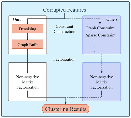
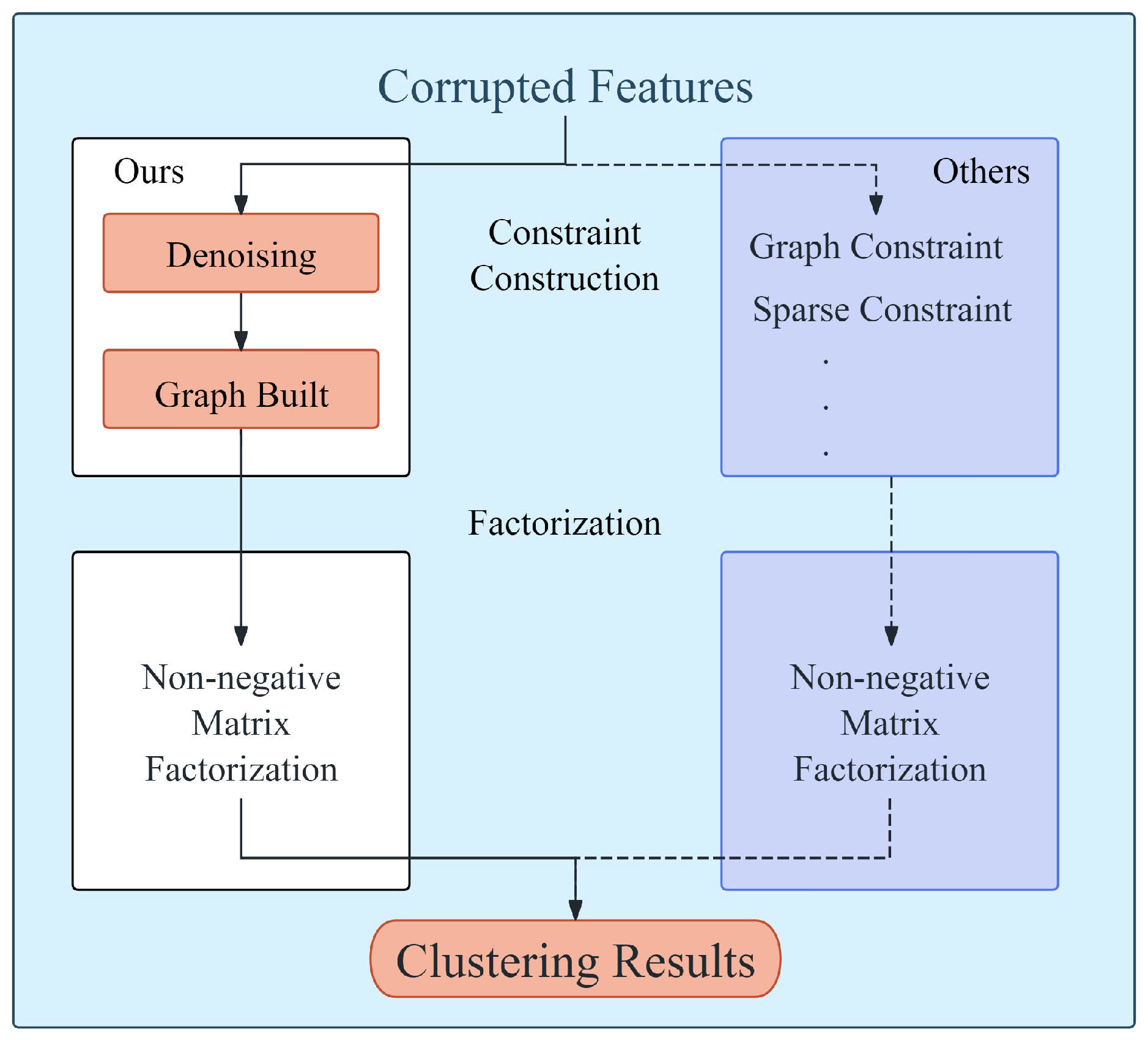
The advantages of deep non-negative matrix factorization in multi-view clustering are obvious: directly obtaining data features, reducing the difficulty in parameter tuning, and matrix factorization without redundancy. However, this also brings corresponding problems: due to directly obtaining features from the data itself, non-negative matrix factorization is more susceptible to noise interference [26,27,28,29,30]. To this end, the authors concatenate the auto-encoder with non-negative matrix factorization, so that the obtained data matrix can still be reconstructed into a cleaned matrix even when it is contaminated by noise, thereby reducing the impact of noise. How our model works and the comparison are shown in Figure 1 below.

Figure 1. Combination of denoising auto-encoder and NMF.

3.2. Features to Similarity Matrix

A multi-view dataset contains features extracted from multiple different perspectives. Due to different angles, simply concatenating or adding features cannot accurately reflect the essence of the data, and instead can lead to confusion. However, although the angles of the samples are different, similar samples often have similar features [21]. Therefore, we choose to use the similarity matrix of sample features rather than the sample features themselves for research.

Considering a dataset where each row serves as a sample, there are various forms of similarity between two samples, including Euler similarity, cosine similarity, etc.

$$\begin{array}{c}\begin{array}{c}{r}_{Eule{r}_{ij}}={\displaystyle \frac{\left|\right|x_i-x_j{\left|\right|}^2}{\left|\right|x_i\left|\right|·\left|\right|x_j\left|\right|}}.\hfill \end{array}\hfill \end{array}$$

(24)

$$\begin{array}{c}\begin{array}{c}{r}_{co{s}_{ij}}={\displaystyle \frac{x_i{\displaystyle x_j^T}}{\left|\right|x_i\left|\right|·\left|\right|x_j\left|\right|}}.\hfill \end{array}\hfill \end{array}$$

(25)

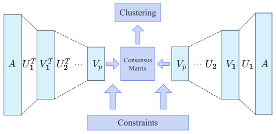
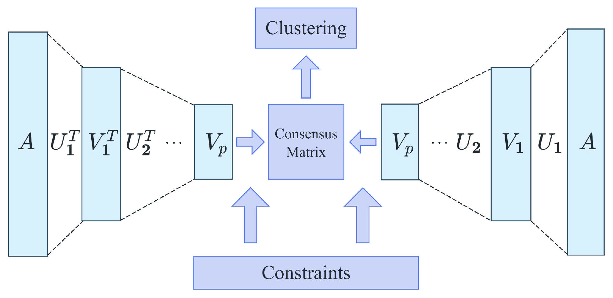
The similarity matrix can be constructed by taking the similarity between sample i and sample j as elements of the matrix. At this point, the similarity matrix is similar to the adjacency matrix of an abstract connected graph—samples belonging to similar or even identical classes have higher similarity and appear as larger elements in the similarity matrix, corresponding to edges with higher weights in an undirected weighted graph. Similarly, samples with lower similarity correspond to edges with lower weights. These can be seen in Figure 2 below.

Figure 2. Using similarity matrix for NMF.

3.3. Matrix to Graph

Subsequently, to further simplify the model, the similarity matrix can be transformed into an undirected and unweighted connected graph. However, using the magnitude of similarity itself as a criterion for preserving edges can bring a series of problems. Due to the tendency of data convergence after DAE processing, it is extremely difficult to simply use similarity values as parameters for preserving edges; at the same time, setting the parameter tuning standard too high can lead to the destruction of the connectivity of the graph, resulting in some points becoming isolated and unable to be discovered by non-negative matrix factorization, which means that clustering will produce redundancy. Meanwhile, if the standard is too low, it can also result in too many edges being retained on the graph, leading to blurry clustering results and even a decrease in the number of clusters.

Because our goal is to find clusters from a cluttered dataset, similar to finding communities from an abstract connected graph, our first concern is the distance between data points, which has already been solved by similarity. Secondly, the authors need specific indicators, which are to divide the data points into two parts based on distance to determine whether they belong to the same community. Using a sigmoid function,

$$f\left(x\right)={\displaystyle \frac{1}{1+e^{-x}}},x\in R$$

(26)

Finally, in order to initialize the size of each cluster reasonably, the authors assume that the size of each cluster is roughly similar, and propose a uniform prior distribution based on this, retaining the most similar points. This can avoid the occurrence of outliers and redundancies caused by too few edges, as well as avoid the blurring of community structure and clustering results caused by forcibly associating originally unrelated points due to too many edges.

4. Experiments

4.1. Datasets Introduction

The authors tested the model on five publicly available online datasets: BBC Sport, 3Sources, Handwritten, Wiki-fea, and Wikipedia. To test the performance of the model, the author used five commonly used indicators: accuracy (ACC), adjusted Rand index (ARI), normalized mutual information (NMI), F-score, and purity. The introduction of the datasets is in the next section. The sources of the datasets are provided at the end of the text.

BBC Sport: This dataset collected 737 articles from BBC Sport News and divided them into 5 categories: athletics, cricket, football, rugby, and tennis. Each piece of data is described in two dimensions. The data itself is arranged in an orderly manner and, during the experiment, it is randomized before clustering.

3Sources: This dataset collected 948 news events from BBC, Reuters, and The Guardian, with each source of information being independently categorized into a separate view. One of the data subsets, which includes 169 articles, is divided into a three-view data subset. The data itself is arranged randomly.

Handwritten: Handwritten digit dataset from the UCI machine learning database. The dataset consists of 2000 images with annotations ranging from 0 to 9. It includes 5 views, each with 6–240 different feature parameters. The data itself is arranged in an orderly manner and, during the experiment, it is randomized before clustering.

Wiki-fea: This dataset is a backup for the recovery of Wiki datasets. It includes a total of 2866 samples, divided into 10 categories. It is an image–text dual-view dataset that contains a total of 10,128 feature values. The data itself is arranged randomly.

Wikipedia: This is a subset of data separated from the Wiki dataset, consisting of a total of 10 different classes. The dataset has two dimensions, including 693 different articles. The data itself is arranged randomly.

4.2. Baseline Algorithm

In order to compare the effectiveness of the models proposed in this article, the author selected 5 proposed algorithms as baseline algorithms.

GMNMF [31]. This algorithm is a further optimization of traditional non-negative matrix factorization. On the basis of non-negative matrix factorization, by introducing the method of local graph regularization, the nearest neighbor graph of nodes is constructed to further obtain the relevant information of nodes and optimize the matrix algorithm. It has more advantages in obtaining data manifolds.

MVCC [32]. This algorithm is also an optimization of non-negative matrix factorization and, compared with GMNMF, it adjusts the processing of data manifolds. It introduces local manifold regularization and adds regularization terms, as well as penalties, which enable it to better preserve the local spatial geometry of data and obtain a consensus solution.

HMVC [33]. This algorithm utilizes high-order information from feature space and topological space, and achieves scalability through graph filtering and anchor-based techniques.

MCVCF [34]. This algorithm extends the method of multi-layer non-negative matrix factorization to each view, revealing the hierarchical structure hidden in the data by decomposing the representation matrix into multiple layers. Meanwhile, the algorithm applies manifold regularization to maintain local consistency in geometry.

GDLMC [35]. This algorithm is a widely used deep clustering algorithm that combines deep learning with multi-view clustering on the basis of non-negative matrix factorization.

4.3. Experimental Results

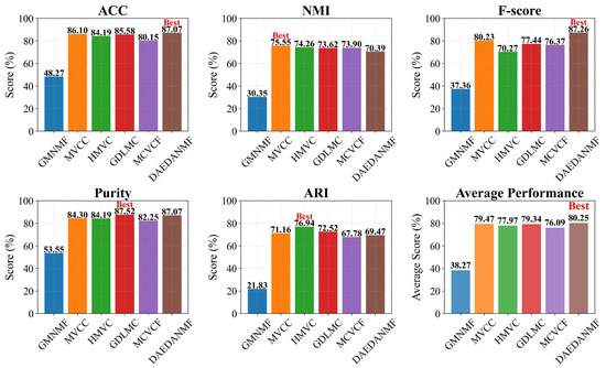
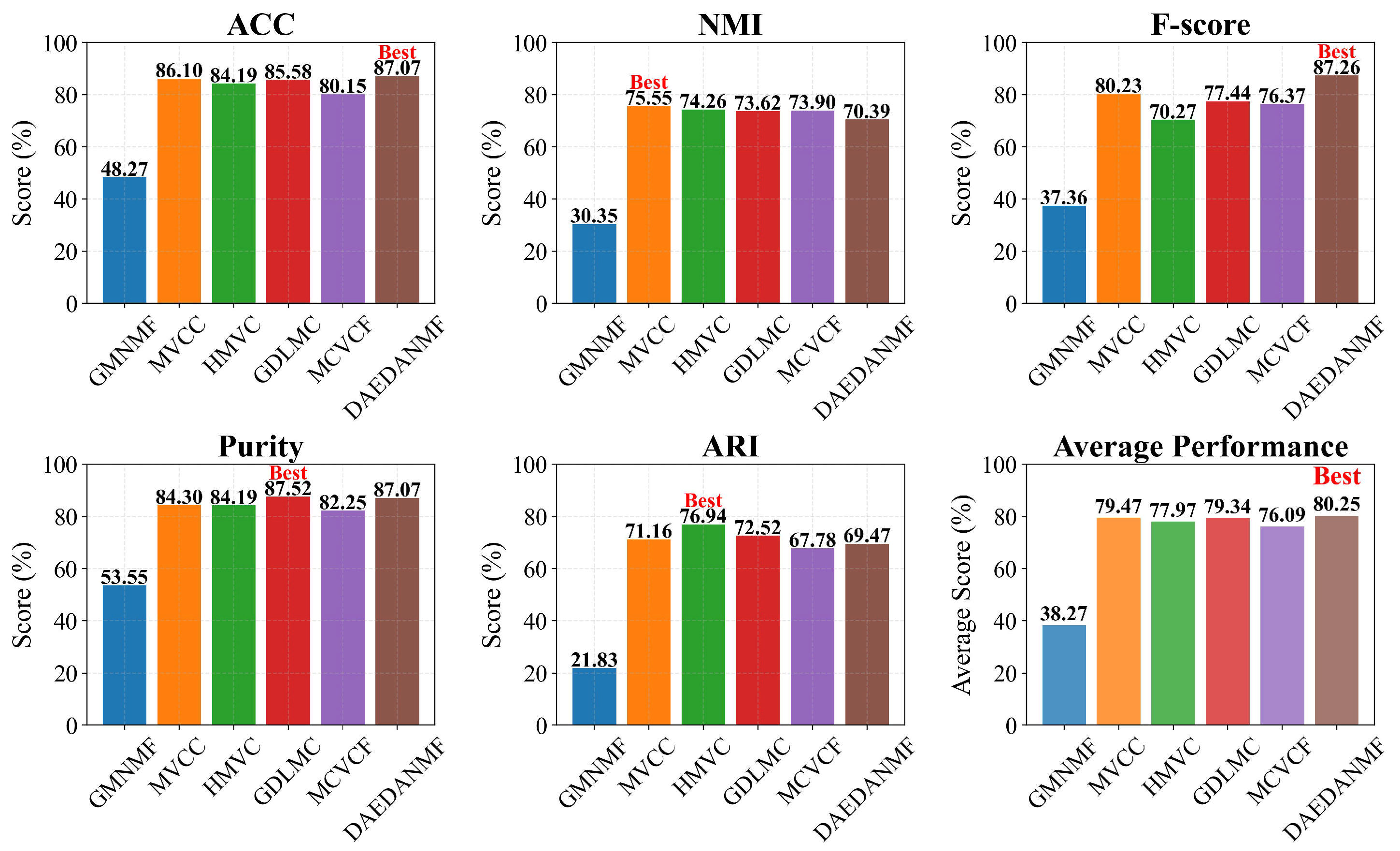
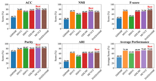
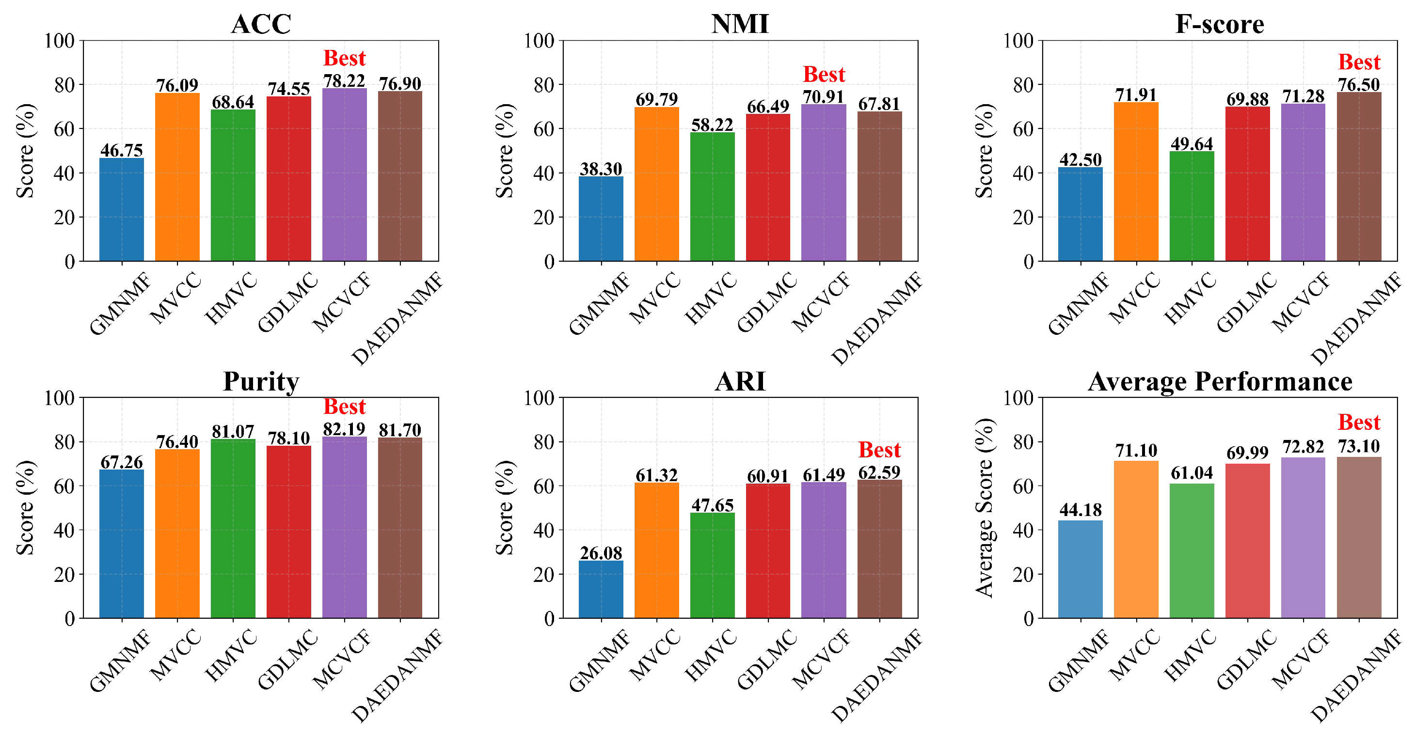
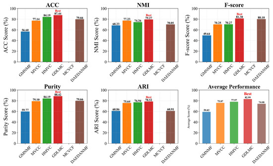
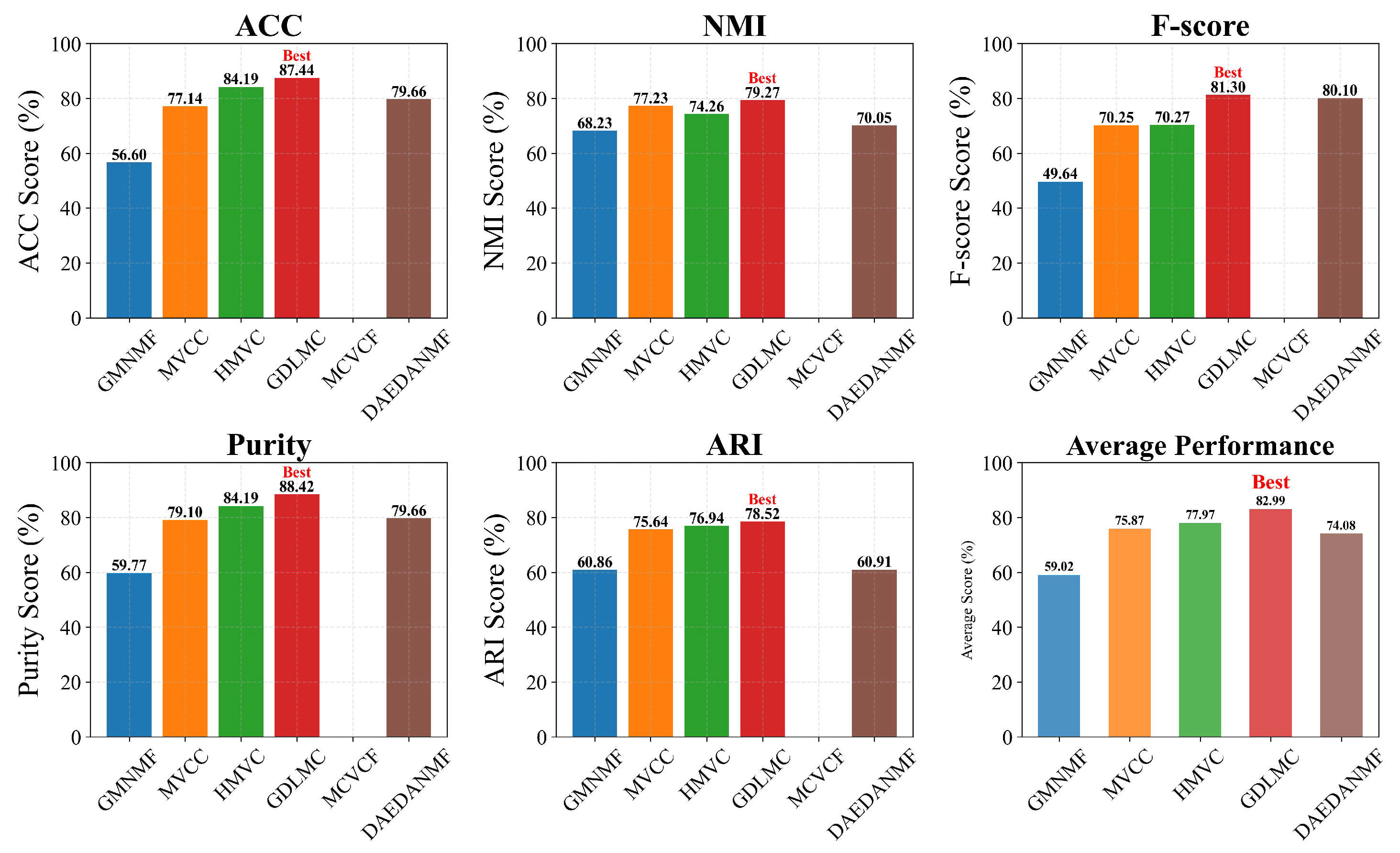
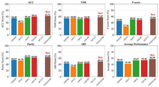
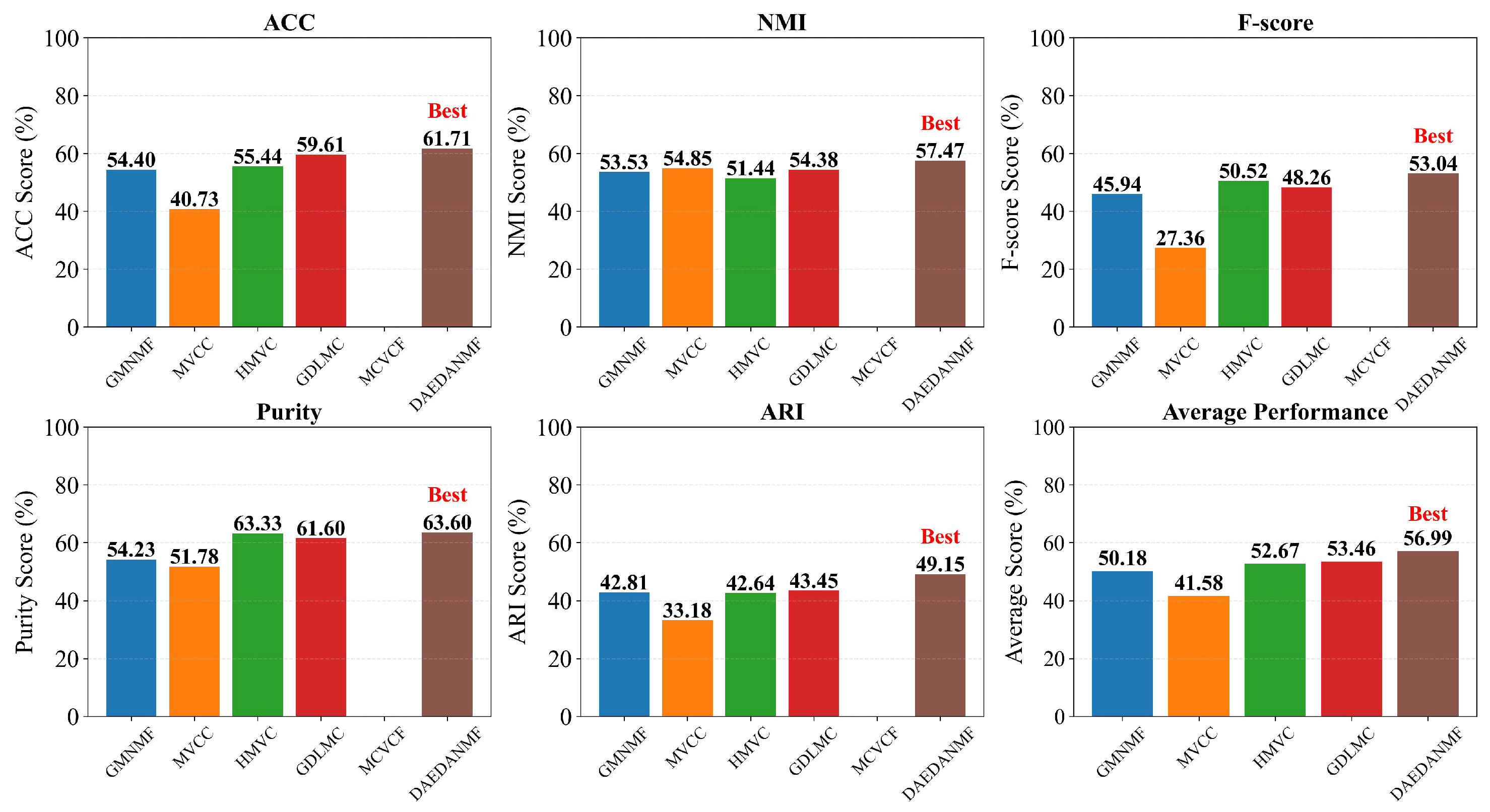
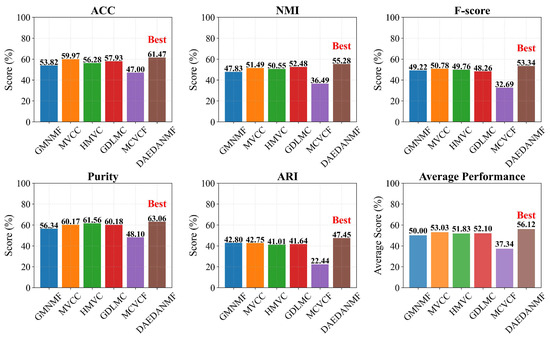
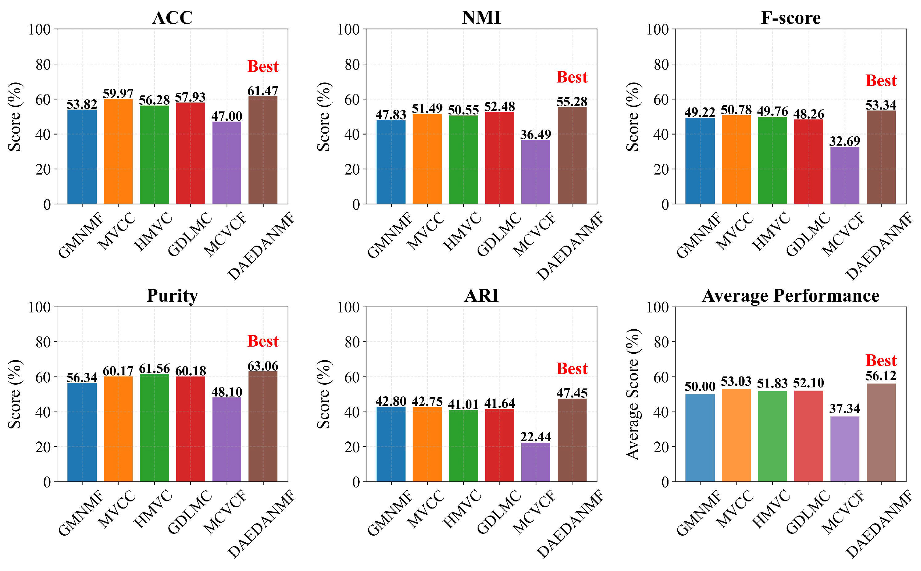
In this part of the experiment, the authors used the original feature matrix to construct an abstract connected graph. By adjusting the parameters, the data that best reflect the similar structural features within the datasets were selected for research. Finally, ACC (accuracy), NMI (normalized mutual information), F-score, Purity (clustering purity), and ARI (adjusted Rand index) were selected as measurement indicators. Table 1, Table 2, Table 3, Table 4 and Table 5 and Figure 3, Figure 4, Figure 5, Figure 6 and Figure 7 show the specific content.

Table 1. Performance evaluation on BBC Sport (The bold format marks out the largest indexes in each column, the upward arrows indicate that the indicators are positively correlated with the performances of the algorithms, the same for the following).

Method	ACC (↑)	NMI (↑)	F-Score (↑)	Purity (↑)	ARI (↑)
GMNMF	48.27	30.35	37.36	53.55	21.83
MVCC	86.10	75.55	80.23	84.30	71.16
HMVC	84.19	74.26	70.27	84.19	76.94
GDLMC	85.58	73.62	77.44	87.52	72.52
MCVCF	80.15	73.90	76.37	82.25	67.78
Ours (DAEDANMF)	87.07	70.39	87.26	87.07	69.47

Table 2. Performance evaluation on 3Sources.

Method	ACC (↑)	NMI (↑)	F-Score (↑)	Purity (↑)	ARI (↑)
GMNMF	46.75	38.30	42.50	67.26	26.08
MVCC	76.09	69.79	71.91	76.40	61.32
HMVC	68.64	58.22	49.64	81.07	47.65
GDLMC	74.55	66.49	69.88	78.10	60.91
MCVCF	78.22	70.91	71.28	82.19	61.49
Ours (DAEDANMF)	76.90	67.81	76.50	81.70	62.59

Table 3. Performance evaluation on Handwritten.

Method	ACC (↑)	NMI (↑)	F-Score (↑)	Purity (↑)	ARI (↑)
GMNMF	56.60	68.23	49.64	59.77	60.86
MVCC	77.14	77.23	70.25	79.10	75.64
HMVC	84.19	74.26	70.27	84.19	76.94
GDLMC	87.44	79.27	81.30	88.42	78.52
MCVCF	—	—	—	—	—
Ours (DAEDANMF)	79.66	70.05	80.10	79.66	60.91

Table 4. Performance evaluation on Wiki-fea.

Method	ACC (↑)	NMI (↑)	F-Score (↑)	Purity (↑)	ARI (↑)
GMNMF	54.40	53.53	45.94	54.23	42.81
MVCC	40.73	54.85	27.36	51.78	33.18
HMVC	55.44	51.44	50.52	63.33	42.64
GDLMC	59.61	54.38	48.26	61.60	43.45
MCVCF	—	—	—	—	—
Ours (DAEDANMF)	61.71	57.47	53.04	63.60	49.15

Table 5. Performance evaluation on Wikipedia.

Method	ACC (↑)	NMI (↑)	F-Score (↑)	Purity (↑)	ARI (↑)
GMNMF	53.82	47.83	49.22	56.34	42.8
MVCC	59.97	51.49	50.78	60.17	42.75
HMVC	56.28	50.55	49.76	61.56	41.01
GDLMC	57.93	52.48	48.26	60.18	41.64
MCVCF	47.00	36.49	32.69	48.10	22.44
Ours (DAEDANMF)	61.47	55.28	53.34	63.06	47.45

Figure 3. Average performance comparison of models on BBC Sport.

Figure 4. Average performance comparison of models on 3Sources.

Figure 5. Average performance comparison of models on Handwritten.

Figure 6. Average performance comparison of models on Wiki-fea.

Figure 7. Average performance comparison of models on Wikipedia.

In this section, to compare the performance of ordinary auto-encoders and denoising auto-encoders, the authors conducted three sets of experiments: using raw data for feature decomposition; adding noise and using a regular auto-encoder to denoise, then performing non-negative matrix factorization and cluster testing; after adding noise, using a denoising auto-encoder to denoise, and then performing non-negative matrix factorization and clustering testing.

For different datasets, the author designed different auto-encoders and set hyper-parameters separately. The relevant parameters are shown in Table 6.

Table 6. Hyper-parameters of the auto-encoder and denoising auto-encoder.

Dataset	Norm & Layers	Epochs	LR *	Batch Size	Activations
Handwritten	01 **, [1024, 256, 64]	400	0.001	256	Relu
Wiki-fea	01 **, [4096, 1024]	400	0.001	256	Relu
Wikipedia	01 **, [1024, 256]	1000	0.001	256	Relu

* LR means learning rate. ** 01 means 0–1 min–max normalization layer.

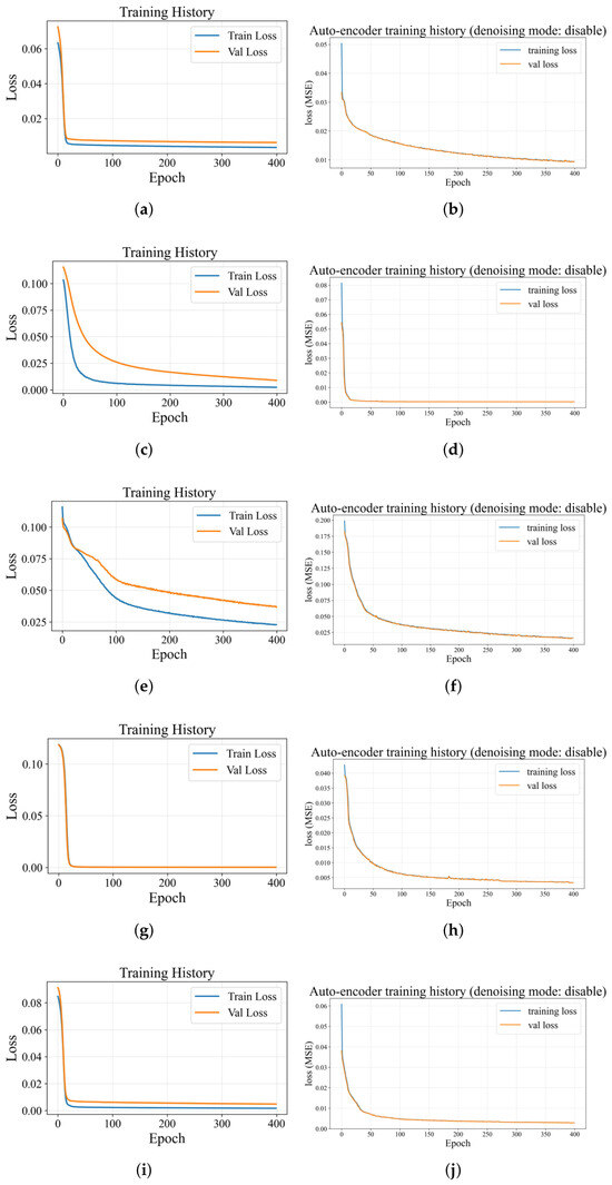
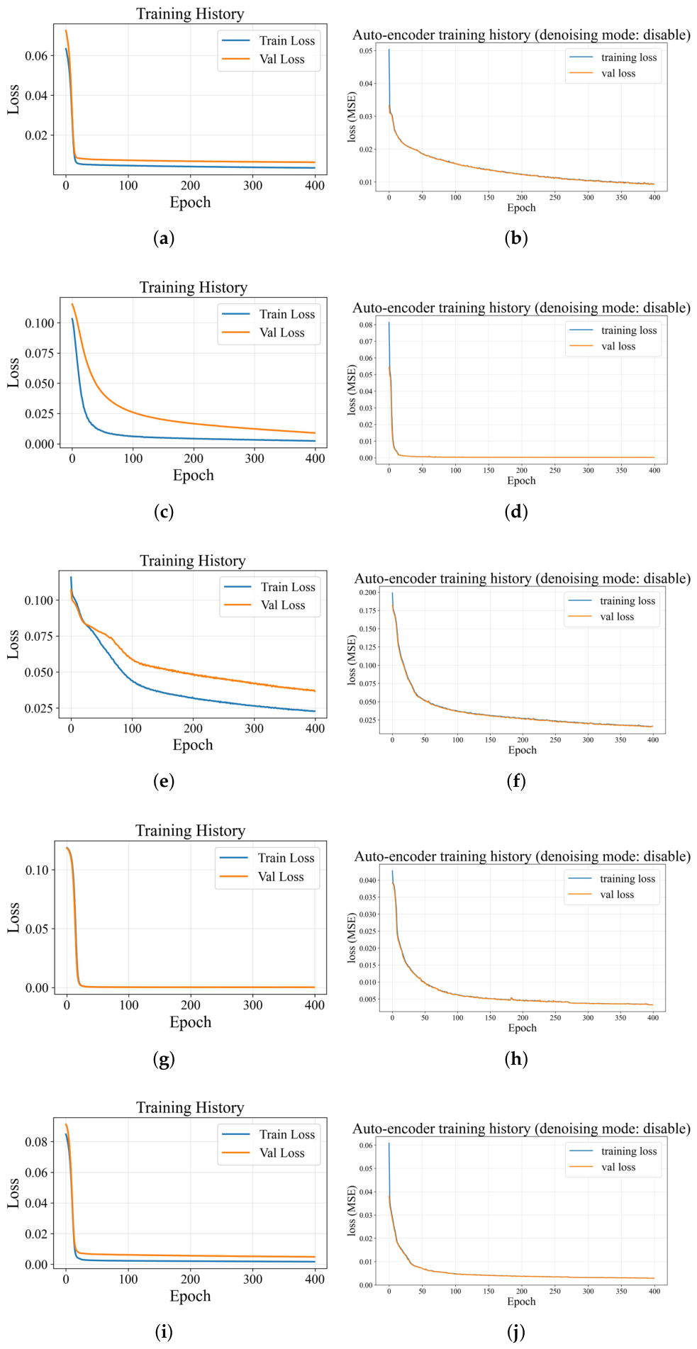
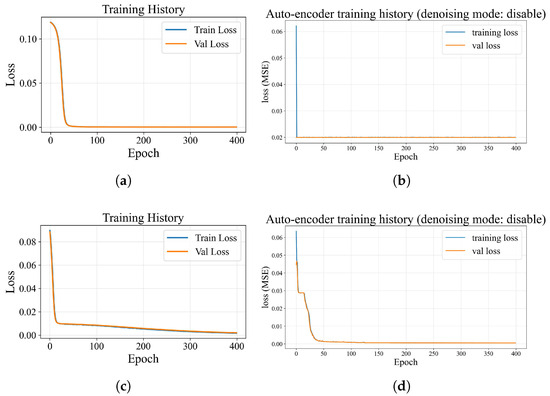
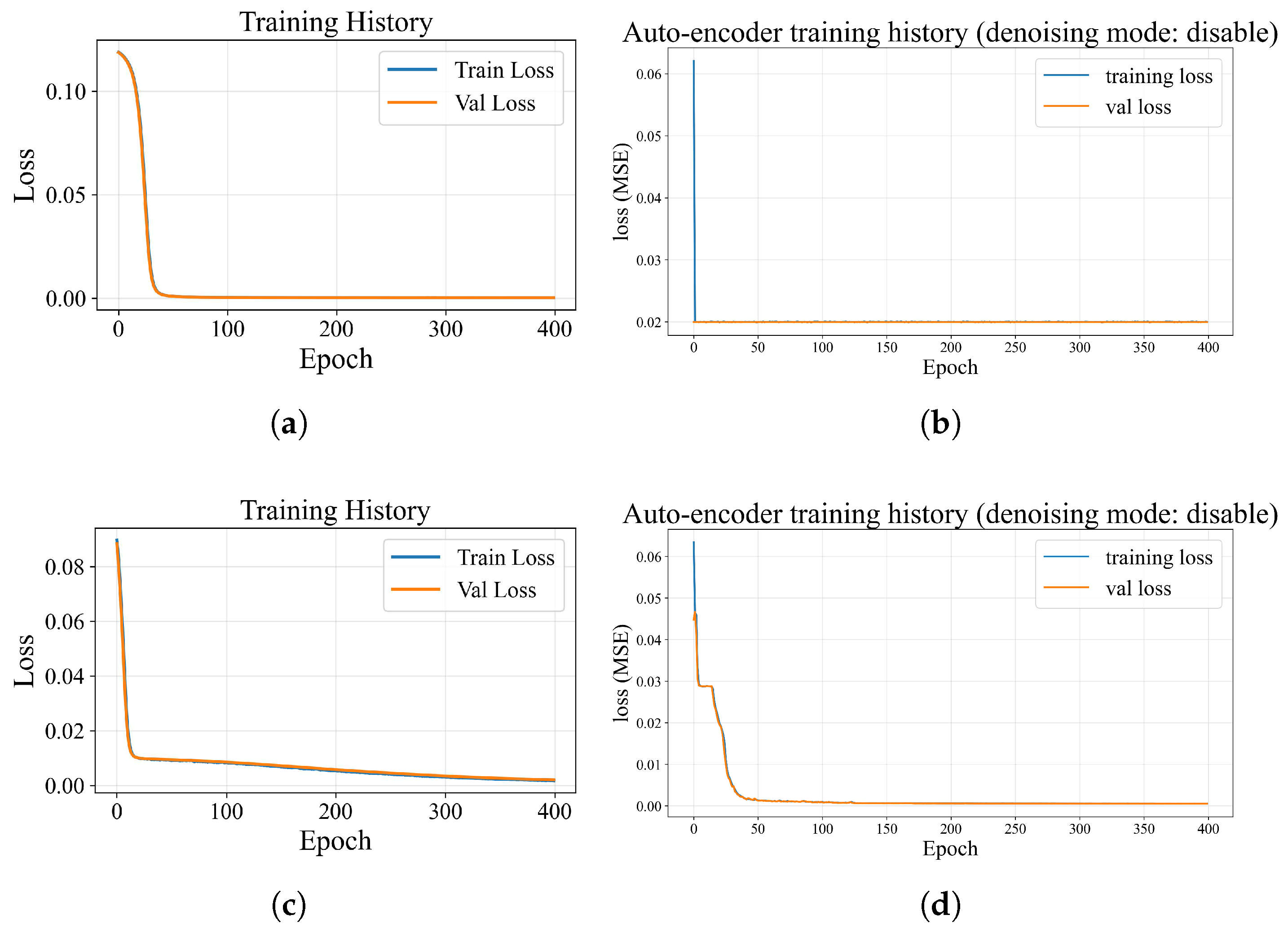
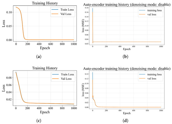
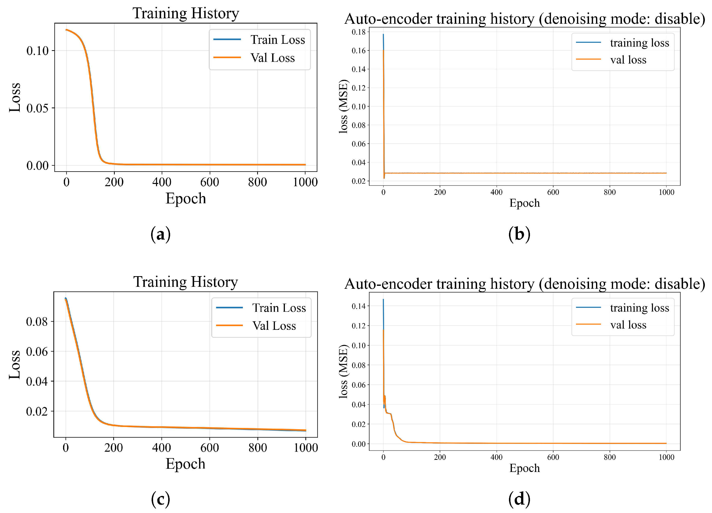
Figure 8, Figure 9 and Figure 10 show the training process and final loss for each view of the three datasets.

Figure 8. Training results of Handwritten dataset. (a) Fourier view: DAE. (b) Fourier view: AE. (c) Mor view: DAE. (d) Mor view: AE. (e) Pixel view: DAE. (f) Pixel view: AE. (g) Profile view: DAE. (h) Profile view: AE. (i) Zer view: DAE. (j) Zer view: AE.

Figure 9. Training results of Wiki-fea dataset. (a) Image view: DAE. (b) Image view: AE. (c) Text view: DAE. (d) Text view: AE.

Figure 10. Training results of Wikipedia dataset. (a) Image view: DAE. (b) Image view: AE. (c) Text view: DAE. (d) Text view: AE.

Table 7, Table 8 and Table 9 show the experimental results of using raw data, adding noise to the raw data combined with a denoising auto-encoder, and adding noise to the raw data combined with a regular auto-encoder on three datasets, Handwritten, Wiki-fea, and Wikipedia. The bold format marks out all the largest results in all columns.

Table 7. The performance results of raw features, cleaned features by AE, and cleaned features by DAE on Handwritten dataset. * Null means neither DAE nor AE has been applied to the data.

Method	ACC (↑)	NMI (↑)	F-Score (↑)	Purity (↑)	ARI (↑)
Null *	66.75	64.07	64.07	72.96	53.00
AE	55.80	63.60	53.50	69.70	48.60
DAE	58.00	61.30	56.90	70.90	46.00

Table 8. The performance results of raw features, cleaned features by AE, and cleaned features by DAE on Wiki-fea dataset. * Null means neither DAE nor AE has been applied to the data.

Method	ACC (↑)	NMI (↑)	F-Score (↑)	Purity (↑)	ARI (↑)
Null *	61.71	57.47	53.04	63.60	49.15
AE	41.34	29.95	38.43	48.25	22.11
DAE	48.32	40.07	41.95	48.78	29.20

Table 9. The performance results of raw features, cleaned features by AE, and cleaned features by DAE on the Wikipedia dataset. * Null means neither DAE nor AE has been applied to the data.

Method	ACC (↑)	NMI (↑)	F-Score (↑)	Purity (↑)	ARI (↑)
Null *	60.69	54.45	53.88	61.71	46.44
AE	48.77	46.14	36.30	50.07	33.08
DAE	50.94	43.38	48.06	52.81	31.97

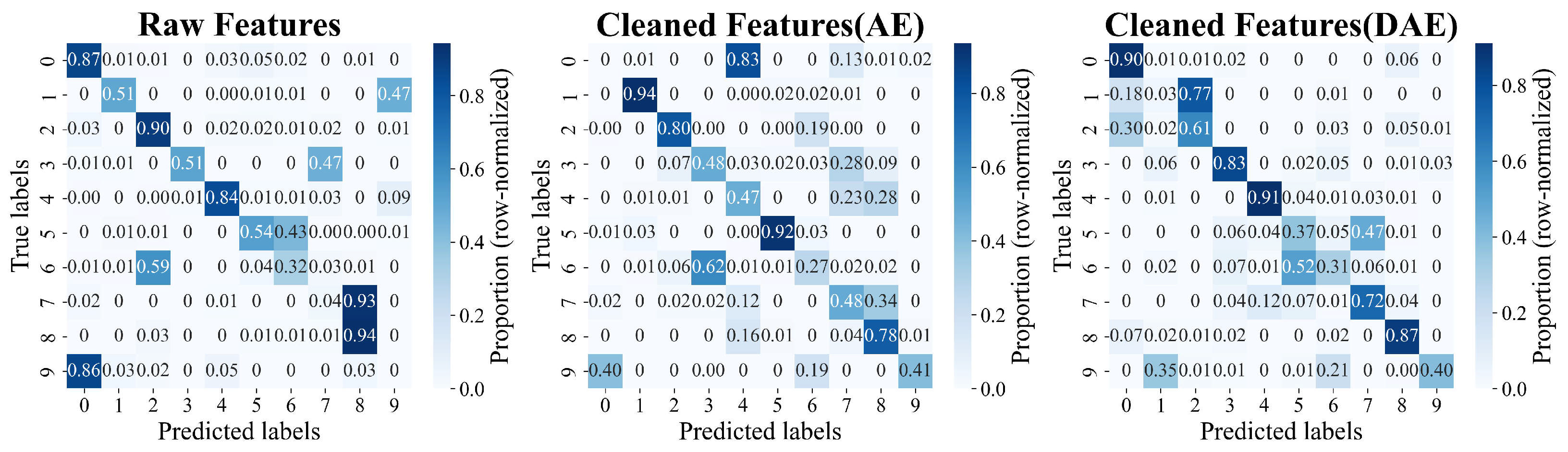
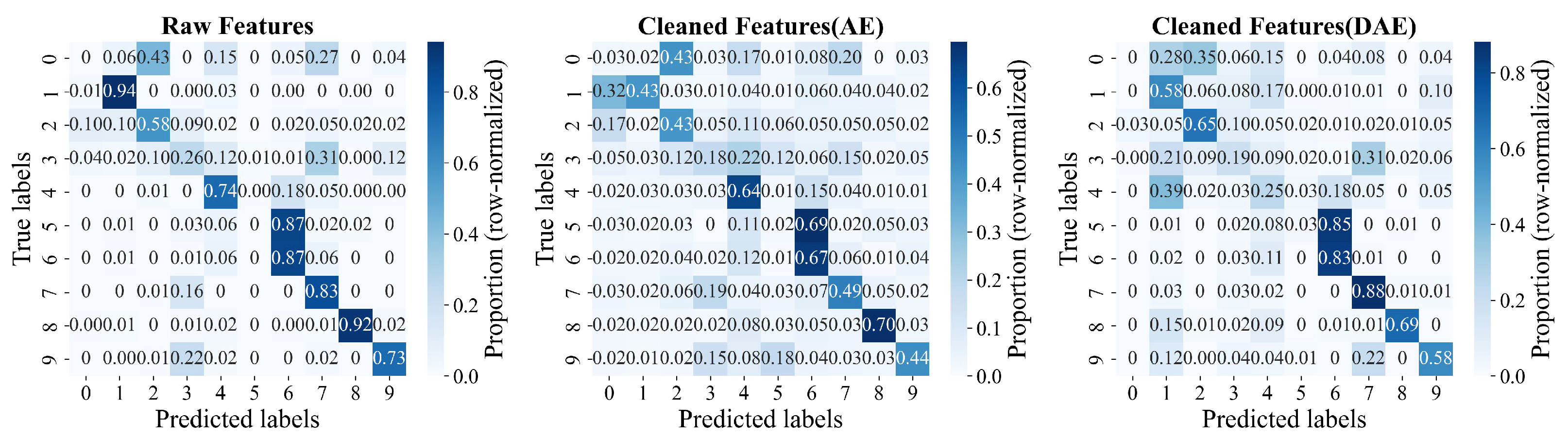
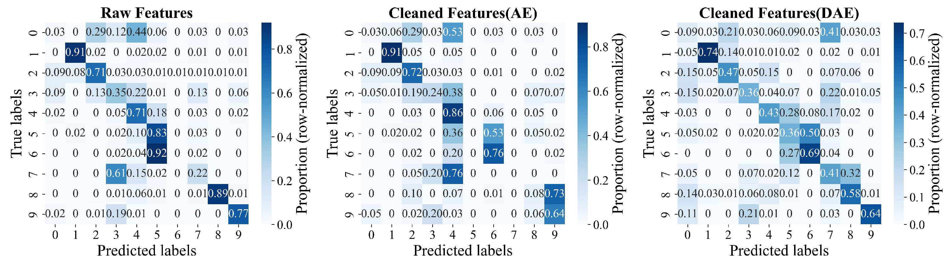
In the clustering confusion matrices, which are represented in Figure 11, Figure 12 and Figure 13, the samples on the diagonal represent correct classification. The zero before the decimal point has been omitted.

Figure 11. The confusion matrices of Handwritten data (the darker the color, the more samples there are, the same for the following).

Figure 12. The confusion matrices of Wiki-fea data.

Figure 13. The confusion matrices of Wikipedia data.

5. Discussion

For different datasets, we selected the most suitable parameters to obtain the best experimental results. Regarding the baseline algorithm we have chosen, we tested the algorithm and code provided in the original paper, and compared the results provided by the original author with those reproduced by other researchers as a benchmark. Detailed index comparisons are in Table 1, Table 2, Table 3, Table 4 and Table 5 and Figure 3, Figure 4, Figure 5, Figure 6 and Figure 7.

Compared with the baseline algorithm, the model constructed in this article achieved better performance on four out of the five datasets used for testing. Among them, on the BBC Sport dataset, this method achieved the highest F-score and overall performance, while on the 3Sources dataset, its ARI and F-score were the highest. On Wiki-fea and the Wikipedia dataset, it achieved the best performance in all five metrics.

After comparing with the baseline algorithm, we conducted comprehensive tests on three datasets: handwritten, Wiki-fea, and Wikipedia. The original datasets were directly used for non-negative matrix decomposition and clustering, denoising auto-encoders were used to denoise and cluster after adding noise, and ordinary auto-encoders were used to denoise and cluster after adding noise. The training processes can be seen in Figure 8, Figure 9 and Figure 10. Finally, the relevant indicators were carefully examined, and they are represented in Table 7, Table 8 and Table 9. All three experiments achieved consistent results: compared with ordinary auto-encoders, the accuracy of auto-encoders increased after denoising, which means that the performance of denoising auto-encoders has been improved compared to ordinary auto-encoders, and they can classify images more accurately. Detailed clustering results are shown as confusion matrices in Figure 11, Figure 12 and Figure 13. At the same time, the clustering purity and F-index have both improved to a certain extent, indicating that the points of each clustering cluster are more compact during feature reconstruction. However, compared to ordinary auto-encoders, denoising auto-encoders use more layers of neural networks and have a more complex structure, resulting in stronger randomness. Therefore, adjusting the Rand coefficient ARI and standardizing the mutual information NMI both slightly decrease accuracy.

Compared to the method of integrating feature extraction and clustering into the same objective function, this paper adopts a concatenated model. Although integrated models may perform better on standardized datasets, their interactions are undoubtedly more complex, and their ability to resist noise will also decrease. In order to improve the robustness of the model, reduce the interaction of various factors, and ensure that each module can operate independently and without interference, the authors adopted a series model. This can not only improve the robustness of the model, but also reduce the mutual interference of various functions. However, to some extent, this does make the model loose and the rigor of the model will also decrease. When put into practical application, a corresponding balance must be struck between the two.

6. Conclusions

In this article, we propose an algorithm, DAEDANMF, designed for clustering multi-view data. We propose the DAEDANMF framework by transplanting machine learning algorithms that search for community structures in abstract graphs to clustering tasks, and combining denoising auto-encoders to mitigate the impact of real-world noise. On the basis of this framework, the authors choose to introduce an alternating iterative algorithm to solve the model. Through this new framework, we effectively integrated data from multiple views and maintained high classification accuracy and robustness on features extracted using different methods.

According to our experimental results, on the one hand, compared with ordinary auto-encoders, the performance of the denoising auto-encoder has improved, indicating that the dedicated denoising auto-encoder performs better in denoising tasks than ordinary auto-encoders. On the other hand, through denoising, the model exhibits good robustness when facing different datasets and can still maintain stability even when the data is contaminated by noise. Meanwhile, when facing data inputs from different views, using the average NMF method instead of the collaborative NMF method can achieve better classification. Future research can focus on two aspects: first, testing the practicality of the model on real-world datasets with noise; secondly, improving the framework of denoising auto-encoders to obtain feature matrices that better represent the data.

References

- Basiri, F.; Amer, A.; Naserabadi, M.; Moghimi, M. A Comparative Study of K-means and NMF Clustering Algorithms. In Proceedings of the 2nd International Engineering Conference on Electrical, Energy, and Artificial Intelligence (EICEEAI), Zarqa, Jordan, 27–28 December 2023. [Google Scholar] [CrossRef] [Scilit]
- Torabi, Y.; Shirani, S.; Reilly, J. Chem-NMF: Multi-layer alpha-divergence Non-Negative Matrix Factorization for Cardiorespiratory Disease Clustering, with Improved Convergence Inspired by Chemical Catalysts and Rigorous Asymptotic Analysis. arXiv 2025, arXiv:2510.06632. [Google Scholar] [CrossRef] [Scilit]
- Mirzal, A. NMF based gene selection algorithm for improving performance of the spectral cancer clustering. In Proceedings of the 2013 IEEE International Conference on Control System, Computing and Engineering, Penang, Malaysia, 29 November–1 December 2013; pp. 74–78. [Google Scholar] [CrossRef] [Scilit]
- Park, S.; Cha, B. Query-Based Multi-Document Summarization Using Non-Negative Semantic Feature and NMF Clustering. In Proceedings of the Fourth International Conference on Networked Computing and Advanced Information Management, Gyeongju, Republic of Korea, 2–4 September 2008; pp. 609–614. [Google Scholar] [CrossRef] [Scilit]
- Lu, X.; Wu, H.; Yuan, Y. Double Constrained NMF for Hyperspectral Unmixing. IEEE Trans. Geosci. Remote Sens. 2014, 52, 2746–2758. [Google Scholar] [CrossRef] [Scilit]
- Rajabi, R.; Ghassemian, H. Spectral Unmixing of Hyperspectral Imagery Using Multilayer NMF. IEEE Geosci. Remote Sens. Lett. 2014, 12, 38–42. [Google Scholar] [CrossRef] [Scilit]
- Goel, D.; Khanna, S. Semi-NMF Regularization-Based Autoencoder Training for Hyperspectral Unmixing. In Proceedings of the 2024 National Conference on Communications (NCC), Chennai, India, 28 February–2 March 2024; pp. 1–6. [Google Scholar] [CrossRef] [Scilit]
- Zhao, J.; Cai, J.; Qu, G.; Wang, C.; Chen, Y. Graph regularized semi-nonnegative matrix factorization under sparse constraints for clustering. Res. Sq. 2024. [Google Scholar] [CrossRef] [Scilit]
- Xu, R.; Li, Y. Wide angle radar imaging under low SNR via sparsity enhanced non-negative matrix factorization. In Proceedings of the 2015 IEEE International Geoscience and Remote Sensing Symposium (IGARSS), Milan, Italy, 26–31 July 2015; pp. 3195–3198. [Google Scholar] [CrossRef] [Scilit]
- Zhong, B.; Wu, J.S.; Huang, W.; Zheng, W.S. Cluster Structure Augmented Deep Nonnegative Matrix Factorization with Low-rank Tensor Learning. Inf. Sci. 2024, 670, 120585. [Google Scholar] [CrossRef] [Scilit]
- Fan, Y.; He, R.; Hu, B.G. Global and local consistent multi-view subspace clustering. In Proceedings of the 3rd IAPR Asian Conference on Pattern Recognition (ACPR), Kuala Lumpur, Malaysia, 3–6 November 2015; pp. 564–568. [Google Scholar] [CrossRef] [Scilit]
- Carel, L.; Alquier, P. Simultaneous Dimension Reduction and Clustering via the NMF-EM Algorithm. Adv. Data Anal. Classif. 2017, 15, 231–260. [Google Scholar] [CrossRef] [Scilit]
- Cho, S. Lee and Seung (2000)’s Algorithms for Non-negative Matrix Factorization: A Supplementary Proof Guide. arXiv 2025, arXiv:2501.11341. [Google Scholar] [CrossRef] [Scilit]
- Liang, J.; Huang, J.; Xi, C.; Wang, Y.; Li, J. JGR-NMF: Joint graph-regularized non-negative matrix factorization for spatial domain identification. PeerJ 2026, 14, e20585. [Google Scholar] [CrossRef] [Scilit]
- Yao, S.; Hu, C.; Wang, T.; Cui, X. Autoencoder-like Semi-NMF Multiple Clustering. Inf. Sci. 2021, 572, 331–342. [Google Scholar] [CrossRef] [Scilit]
- Bhattamishra, S. Deep Probabilistic NMF Using Denoising Autoencoders. Int. J. Mach. Learn. Comput. 2018, 8, 49–53. [Google Scholar] [CrossRef] [Scilit]
- Ye, F.; Chen, C.; Zheng, Z. Deep Autoencoder-like Nonnegative Matrix Factorization for Community Detection. In CIKM ’18: Proceedings of the 27th ACM International Conference on Information and Knowledge Management; Association for Computing Machinery: New York, NY, USA, 2018; pp. 1393–1402. [Google Scholar] [CrossRef] [Scilit]
- Salha-Galvan, G.; Hennequin, R.; Vazirgiannis, M. Simple and Effective Graph Autoencoders with One-Hop Linear Models. In Machine Learning and Knowledge Discovery in Databases; Springer: Cham, Switzerland, 2021; pp. 319–334. [Google Scholar] [CrossRef] [Scilit]
- Seghair, T.; Besbes, O.; Abdellatif, T.; Bihiri, S. VQ-VGAE: Vector Quantized Variational Graph Auto-Encoder for Unsupervised Anomaly Detection. In Proceedings of the 2024 IEEE International Conference on Big Data (BigData), Washington, DC, USA, 15–18 December 2024; pp. 2370–2375. [Google Scholar] [CrossRef] [Scilit]
- Liu, G.; Ge, H.; Li, T.; Su, S.; Gao, P. Multi-view clustering via diversity induction and multi-layer concept factorization. Pattern Anal. Appl. 2025, 28, 76. [Google Scholar] [CrossRef] [Scilit]
- Wang, W.; Chen, F.; Ge, Y.; Huang, S.; Zhang, X.; Yang, D. Discriminative Deep Semi-Nonnegative Matrix Factorization Network with Similarity Maximization for Unsupervised Feature Learning. Pattern Recognit. Lett. 2021, 149, 157–163. [Google Scholar] [CrossRef] [Scilit]
- Vincent, P.; Larochelle, H.; Manzagol, P.A. Extracting and composing robust features with denoising autoencoders. In ICML ’08: Proceedings of the 25th International Conference on Machine Learning; Association for Computing Machinery: New York, NY, USA, 2008; pp. 1096–1103. [Google Scholar] [CrossRef] [Scilit]
- Zhang, C.; Yang, F.; Yang, J. Basis Clustering Regularized NMF for Multichannel Blind Source Separation. IEEE Trans. Audio Speech Lang. Process. 2026, 34, 153–168. [Google Scholar] [CrossRef] [Scilit]
- Jaiswal, R.; Fitzgerald, D.; Barry, D.; Coyle, E.; Rickard, S. Clustering NMF basis functions using Shifted NMF for monaural sound source separation. In Proceedings of the 2011 IEEE International Conference on Acoustics, Speech and Signal Processing (ICASSP), Prague, Czech Republic, 22–27 May 2011; pp. 245–248. [Google Scholar] [CrossRef] [Scilit]
- Redko, I.; Bennani, Y. Controlling Orthogonality Constraints for Better NMF Clustering. In Proceedings of the 2014 International Joint Conference on Neural Networks (IJCNN), Beijing, China, 6–11 July 2014. [Google Scholar] [CrossRef] [Scilit]
- Plis, S.; Potluru, V.; Lane, T.; Calhoun, V. Correlated noise: How it Breaks NMF, and What to Do about it. Signal Process. Syst. 2011, 65, 351–359. [Google Scholar] [CrossRef] [Scilit]
- Vaghmare, A.; Rama Rao, C. Unsupervised noise removal technique based on constrained NMF. IET Signal Process. 2017, 11, 788–795. [Google Scholar] [CrossRef] [Scilit]
- Tian, Y.; Li, Y.; Lin, H.; Ma, H. A sparse NMF-SU for seismic random noise attenuation. IEEE Geosci. Remote Sens. Lett. 2013, 10, 607–611. [Google Scholar] [CrossRef] [Scilit]
- Barkhoda, W.; Seyedi, A.; Gillis, N.; Akhlaghian Tab, F. Instance-wise distributionally robust nonnegative matrix factorization. Pattern Recognit. 2025, 169, 111732. [Google Scholar] [CrossRef] [Scilit]
- Park, S.; Seok, J.; Hong, J. Probabilistic Noise Detection and Weighted Non-Negative Matrix Factorization-Based Noise Reduction Methods for Snapping Shrimp Noise. J. Mar. Sci. Eng. 2025, 13, 96. [Google Scholar] [CrossRef] [Scilit]
- Wang, Z.; Kong, X.; Fu, H.; Li, M.; Zhang, Y. Feature extraction via multi-view non-negative matrix factorization with local graph regularization. In Proceedings of the 2015 IEEE International Conference on Image Processing (ICIP), Quebec, QC, Canada, 27–30 September 2015; pp. 3500–3504. [Google Scholar] [CrossRef] [Scilit]
- Khan, G.; Hu, J.; Li, T.; Diallo, B.; Wang, H. Multi-view data clustering via non-negative matrix factorization with manifold regularization. Int. J. Mach. Learn. Cybern. 2022, 13, 677–689. [Google Scholar] [CrossRef] [Scilit]
- Pan, E.; Kang, Z. High-order Multi-view Clustering for Generic Data. arXiv 2022, arXiv:2209.10838. [Google Scholar] [CrossRef] [Scilit]
- Chang, S.; Hu, J.; Li, T.; Wang, H.; Peng, B. Multi-view clustering via deep concept factorization. Knowl.-Based Syst. 2021, 217, 106807. [Google Scholar] [CrossRef] [Scilit]
- Wang, D.; Li, T.; Deng, P.; Liu, J.; Huang, W.; Zhang, F. A Generalized Deep Learning Algorithm Based on NMF for Multi-View Clustering. IEEE Trans. Big Data 2022, 9, 328–340. [Google Scholar] [CrossRef] [Scilit]
Disclaimer/Publisher’s Note: The statements, opinions and data contained in all publications are solely those of the individual author(s) and contributor(s) and not of MDPI and/or the editor(s). MDPI and/or the editor(s) disclaim responsibility for any injury to people or property resulting from any ideas, methods, instructions or products referred to in the content. |
© 2026 by the authors. Licensee MDPI, Basel, Switzerland. This article is an open access article distributed under the terms and conditions of the Creative Commons Attribution (CC BY) license.