Design and Comparative Evaluation of Path-Tracking Controllers Using Reduced-Order State-Space Models

Abstract

This study presents a comparative evaluation of path-tracking controllers designed from reduced-order state-space vehicle models. A four-state state-space model is formulated from the bicycle-model dynamics and target-path geometry, where the state variables are the previewed lateral error, heading error, side-slip angle, and yaw rate. To reduce the dependence on variables that are difficult to obtain in practice, a three-state model is derived by eliminating the explicit side-slip dynamics, and a two-state model is further obtained by replacing the yaw-rate dynamics with a kinematic approximation. Based on these three models, linear-quadratic regulator (LQR) controllers are designed. In addition, two linear quadratic static output-feedback (LQ SOF) controllers are constructed from the original four-state model by using reduced output sets. The five controllers are evaluated by vehicle simulations carried out in CarSim under front-wheel-steering and four-wheel-steering configurations. The results clarify the influence of controller structure and model order on path-tracking performance and identify the controller–actuator combination that provides the most favorable performance under the conditions considered.

1. Introduction

Autonomous driving has received sustained research interest because of its potential to improve traffic safety, reduce driver workload, and enhance transportation efficiency [1,2,3]. In a typical autonomous-driving system, perception, planning, and control constitute the main functional modules, and the control module determines how accurately the vehicle follows a prescribed path. Accordingly, path tracking is a key function in automated driving systems [4,5,6,7,8,9,10].

The path-tracking performance of a controller is closely related to the vehicle model used in the controller design stage. Existing path-tracking models can be broadly classified into two categories. The first category is based mainly on the lateral offset error e_y, heading error e_ψ, and their derivatives [11,12,13,14,15,16,17]. The second category additionally incorporates vehicle dynamic states, such as yaw rate γ and side-slip angle β, together with the tracking errors [18,19,20,21,22,23,24,25,26,27,28,29,30,31,32]. In this study, the latter category is adopted because it can represent lateral dynamic behavior more explicitly and is therefore more suitable for maneuvers in which yaw response and lateral stability are important, such as obstacle avoidance or low-friction driving [18,21,25,26,29,30,32]. The latter model, which includes (e_y, e_ψ, β, γ) is referred to hereafter as the four-state state-space model.

Although a four-state model including e_y, e_ψ, β and γ provides a physically meaningful description of path-tracking dynamics, its practical implementation is limited by the difficulty of obtaining reliable side-slip information in real vehicles. One possible solution is to use static output feedback (SOF) in place of full-state feedback. In previous studies, LQ SOF controllers were designed by selecting reduced output sets from the original four-state model [32,33,34,35,36,37]. In that study, two output sets, (e_y, e_ψ) and (e_y, e_ψ, γ), were selected for SOF design, and the corresponding LQ SOF controllers were then obtained [32]. However, unlike LQR design, LQ SOF design requires a heuristic optimization procedure. To avoid this difficulty, this study derives reduced-order state-space models directly from the four-state formulation and then designs LQR controllers based on those simplified models.

Two steering configurations are considered in this work, namely front-wheel steering (FWS) and four-wheel steering (4WS). Other motion-control actuators, including rear-wheel steering and four-wheel independent braking/driving, have also been discussed in previous studies on vehicle motion control on low-friction surfaces [30,31,32]. Nevertheless, they are not included here because earlier results indicated that their contribution to path-tracking improvement is relatively limited in the present context [31,32].

In terms of practical implementation, FWS is more favorable because it depends on the conventional front steering hardware architecture already established in production vehicles. By comparison, 4WS requires additional rear steering hardware and supervisory coordination between the front and rear steering systems. Hence, while 4WS is practically realizable and can improve maneuverability and path-tracking performance, these benefits are accompanied by increased hardware complexity, packaging constraints, calibration burden, and cost.

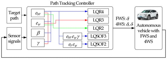
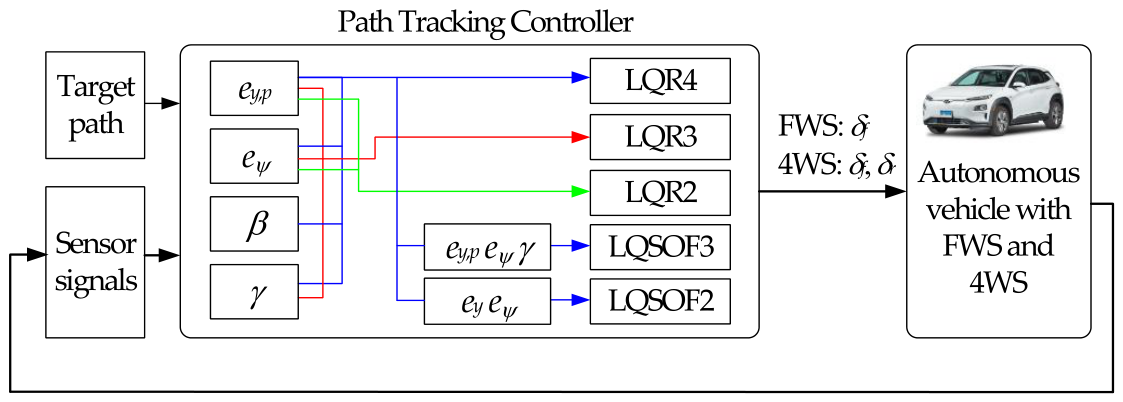
The objective of this paper is to formulate and compare several path-tracking controller structures obtained from vehicle models with different levels of complexity. Figure 1 illustrates the overall procedure for designing the path-tracking controllers considered in this study. Starting from the original four-state state-space model, a reduced three-state model with (e_y, e_ψ, γ) is derived by assuming that β is constant or varies slowly. For simplicity, a two-state reduced state-space model with (e_y, e_ψ) is derived by assuming that γ is determined kinematically by the steering input. LQR controllers based on these three state-space models are then developed and denoted as LQR4, LQR3, and LQR2 in Figure 1, respectively. For comparison, two LQ SOF controllers are also designed from the four-state state-space model by using the output sets, (e_y, e_ψ, γ) and (e_y, e_ψ), and these controllers are denoted as LQSOF3 and LQSOF2 in Figure 1, respectively. Both FWS and 4WS are considered actuator configurations, and CarSim-based simulations are conducted to identify the controller–actuator combination that yields the best path-tracking performance.

Figure 1. Control structure of LQR and LQ controllers for path tracking.

Unlike the previous study, in which LQ SOF controllers were designed from the original four-state state-space model using reduced output sets, the present study investigates the effect of the controller design model order itself on path-tracking performance. To this end, three-state and two-state control-oriented models are explicitly derived from the four-state formulation, and full-state LQR controllers, namely LQR4, LQR3, and LQR2, are designed from the corresponding models. These controllers are then compared with previously developed LQSOF3 and LQSOF2 controllers under the same CarSim environment [32]. Therefore, the novelty of this study lies in the systematic comparison of two different controller simplification strategies, namely model-order reduction and output-feedback reduction, and in providing practical insight into their performance–complexity trade-off for vehicle path tracking.

The remainder of this paper is organized as follows. Section 2 describes the derivation of the state-space models and the design procedures for the LQR and LQ SOF controllers. Section 3 introduces the performance indices used for quantitative evaluation. Section 4 presents and discusses the simulation results. Finally, Section 5 summarizes the main conclusions.

2. Controller Design for Path Tracking

2.1. Formulation of the State-Space Models

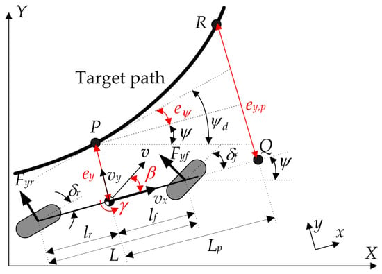
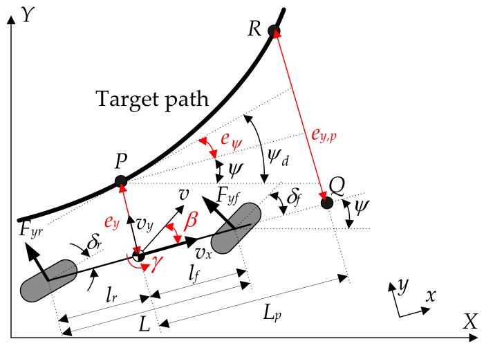
For controller design, the lateral and yaw motions of the vehicle are represented by a two-degree-of-freedom planar bicycle model [12,14,15,16,17,18,19,21,23,26,28,29,30,31,38]. Figure 2 shows the geometric representation of the bicycle model, including the relevant parameters and the target path. This representation is widely used because it captures the dominant lateral and yaw motions while keeping the mathematical structure suitable for controller synthesis. The longitudinal speed v_x is assumed to remain constant during the maneuver [38,39]. The main dynamic variables are selected as the side-slip angle β and yaw rate γ. By applying the lateral-force and yaw-moment balances to the vehicle body, the governing equations are obtained as (1) [17,29,30,31,32,38]. The front and rear tire slip angles, α_f and α_r, are then expressed as (2) in terms of the vehicle states, and the corresponding lateral tire forces, F_yf and F_yr, are approximated as (3) by linear cornering-stiffness relations. Combining these relations leads to the linear vehicle model, (4).

$$\left\{\begin{array}{l}m{v}_x\left(\dot{\beta }+\mathsf{\gamma }\right)=F_{yf}+F_{yr}\\ I_z\dot{\mathsf{\gamma }}=l_f{F}_{yf}-l_r{F}_{yr}\end{array}\right.$$

(1)

$$\left\{\begin{array}{l}{\alpha }_f={\delta }_f-{\tan }^{-1}\left(\beta +{\displaystyle \frac{l_f\mathsf{\gamma }}{v_x}}\right)\approx {\delta }_f-\beta -{\displaystyle \frac{l_f\mathsf{\gamma }}{v_x}}\\ {\alpha }_r={\delta }_r-{\tan }^{-1}\left(\beta -{\displaystyle \frac{l_r\mathsf{\gamma }}{v_x}}\right)\approx {\delta }_r-\beta +{\displaystyle \frac{l_r\mathsf{\gamma }}{v_x}}\end{array}\right.$$

(2)

$$F_{yf}=C_f{\alpha }_f,\hspace{1em}{F}_{yr}=C_r{\alpha }_r$$

(3)

$$\begin{array}{l}\dot{\beta }=\left({\displaystyle \frac{{\varsigma }_1}{m{v}_x}}\right)\beta +\left({\displaystyle \frac{{\varsigma }_2}{m{v}_x^2}}-1\right)\mathsf{\gamma }+{\displaystyle \frac{C_f}{m{v}_x}}{\delta }_f+{\displaystyle \frac{C_r}{m{v}_x}}{\delta }_r\\ \dot{\mathsf{\gamma }}=\left({\displaystyle \frac{{\varsigma }_2}{I_z}}\right)\beta +\left({\displaystyle \frac{{\varsigma }_3}{I_z{v}_x}}\right)\mathsf{\gamma }+{\displaystyle \frac{l_f{C}_f}{I_z}}{\delta }_f-{\displaystyle \frac{l_r{C}_r}{I_z}}{\delta }_r\\ {\varsigma }_1=-C_f-C_r, {\varsigma }_2=-C_f{l}_f+C_r{l}_r, {\varsigma }_3=-l_f^2{C}_f-l_r^2{C}_r\end{array}$$

(4)

Figure 2. Geometric representation of the bicycle model, including the relevant parameters and the target path.

To define the path-tracking problem, the lateral error e_y and heading error e_ψ are introduced with respect to the target path. In addition to the nominal tracking point, a preview point is adopted so that the controller can respond to the path ahead of the vehicle rather than only to the local instantaneous error [12,13,17,18,21,29,30,31,32]. This preview strategy is particularly important on low-friction surfaces.

The preview distance L_p is defined by (5) through the gain k_v. Using this distance, the preview point Q and the corresponding point R on the target path are determined. The desired heading angle at point P is denoted by ψ_d, and the heading error e_ψ is defined as (6) accordingly. The previewed lateral error e_y,p is then obtained by using L_p. Under the small-angle assumption, the kinematic relations for e_y, e_y,p, and e_ψ are derived as (8), where the path curvature κ is treated as an external disturbance.

$$L_p=k_v\cdot v_x$$

(5)

$$e_{\psi }=\psi -{\psi }_d$$

(6)

$$e_{y,p}=e_y+L_p{e}_{\psi }$$

(7)

$$\left\{\begin{array}{l}{\dot{e}}_y=v_x\beta +v_x\sin \left(e_{\psi }\right)\approx v_x\beta +v_x{e}_{\psi }\hfill \\ {\dot{e}}_{\psi }=\dot{\psi }-{\dot{\psi }}_d=\mathsf{\gamma }-v_x\kappa \hfill \\ {\dot{e}}_{y,p}={\dot{e}}_y+L_p{\dot{e}}_{\psi }=v_x\beta +v_x{e}_{\psi }+L_p\mathsf{\gamma }-L_p{v}_x\kappa \hfill \end{array}\right.$$

(8)

Using the four state variables e_y,p, e_ψ, β and γ, the state vector of the four-state model is defined as x₄ in (9). Since two steering configurations are considered, the control input vector is specified as (10) according to whether FWS or 4WS is used. By combining the definitions (9) and (10) with the vehicle dynamics (4) and path-tracking kinematics (8), the four-state state-space model is obtained as (11), where the matrices A₄, D₄ and B₄, are given in (12). The input matrix B₄ of (11) corresponds to 4WS. If FWS is selected as an actuator, the first column of B₄ is used. This model is denoted as SSM4.

$$x_4={\left[\begin{array}{cccc}{e}_{y,p}& e_{\psi }& \beta & \mathsf{\gamma }\end{array}\right]}^T,\hspace{1em}w=\kappa$$

(9)

$$u\in \left\{u_{FWS},u_{4WS}\right\},\hspace{1em}\left\{\begin{array}{l}{u}_{FWS}={\delta }_f\hfill \\ u_{4WS}={\left[\begin{array}{cc}{\delta }_f& {\delta }_r\end{array}\right]}^T\hfill \end{array}\right.$$

(10)

$${\dot{x}}_4=A_4{x}_4+D_{4}w+B_4\mathbf{u}$$

(11)

$$A_4=\left[\begin{array}{cccc}0& v_x& v_x& L_p\\ 0& 0& 0& 1\\ 0& 0& {\displaystyle \frac{{\varsigma }_1}{m{v}_x}}& {\displaystyle \frac{{\varsigma }_2}{m{v}_x^2}}-1\\ 0& 0& {\displaystyle \frac{{\varsigma }_2}{I_z}}& {\displaystyle \frac{{\varsigma }_3}{I_z{v}_x}}\end{array}\right],\hspace{1em}{D}_4=\left[\begin{array}{c}-v_x{L}_p\\ -v_x\\ 0\\ 0\end{array}\right],\hspace{1em}{B}_4=\left[\begin{array}{ll}0\hfill & 0\hfill \\ 0\hfill & 0\hfill \\ {\displaystyle \frac{C_f}{m{v}_x}}\hfill & {\displaystyle \frac{C_r}{m{v}_x}}\hfill \\ {\displaystyle \frac{l_f{C}_f}{I_z}}\hfill & -{\displaystyle \frac{l_r{C}_r}{I_z}}\hfill \end{array}\right]$$

(12)

In real vehicle applications, reliable direct measurement of the side-slip angle β is difficult. Therefore, the use of SSM4 requires a state estimator [40]. To avoid estimating β, a three-state reduced state-space model is constructed with three states e_y,p, e_ψ and γ. For this purpose, the quasi-steady condition on β is assumed as $\dot{\beta }\simeq 0$.

The quasi-steady assumption for β means that β evolves much faster than e_y,p and e_ψ and therefore can be approximated as an algebraic variable rather than an independent dynamic state. Physically, this corresponds to the situation in which the lateral tire forces quickly balance the lateral/yaw motion, so that $\dot{\beta }\simeq 0$ is a reasonable approximation. This is typically acceptable during mild-to-moderate cornering, with small tire slip angles, approximately constant longitudinal speed, and no aggressive transient maneuver. In other words, the assumption is suitable when the vehicle operates away from the handling limits and the lateral dynamics are dominated by near-linear tire behavior.

Applying this assumption to the first equation in (4) yields (13). Multiplying (13) by mv_x and rearranging the result gives (14). By replacing β in (4) and (8) with (14), (15) is obtained.

$$0=\left({\displaystyle \frac{{\varsigma }_1}{m{v}_x}}\right)\beta +\left({\displaystyle \frac{{\varsigma }_2}{m{v}_x^2}}-1\right)\mathsf{\gamma }+{\displaystyle \frac{C_f}{m{v}_x}}{\delta }_f+{\displaystyle \frac{C_r}{m{v}_x}}{\delta }_r$$

(13)

$$\beta =-{\displaystyle \frac{\left(\frac{{\varsigma }_2}{v_x}-m{v}_x\right)}{{\varsigma }_1}}\mathsf{\gamma }-{\displaystyle \frac{C_f}{{\varsigma }_1}}{\delta }_f-{\displaystyle \frac{C_r}{{\varsigma }_1}}{\delta }_r\equiv {\sigma }_{\mathsf{\gamma }}\mathsf{\gamma }+{\sigma }_f{\delta }_f+{\sigma }_r{\delta }_r$$

(14)

$$\left\{\begin{array}{l}\dot{\mathsf{\gamma }}=\left({\displaystyle \frac{{\sigma }_{\mathsf{\gamma }}{\varsigma }_2}{I_z}}+{\displaystyle \frac{{\varsigma }_3}{I_z{v}_x}}\right)\mathsf{\gamma }+\left({\displaystyle \frac{{\sigma }_f{\varsigma }_2}{I_z}}+{\displaystyle \frac{l_f{C}_f}{I_z}}\right){\delta }_f+\left({\displaystyle \frac{{\varsigma }_3}{I_z{v}_x}}-{\displaystyle \frac{l_r{C}_r}{I_z}}\right){\delta }_r\hfill \\ {\dot{e}}_{y,p}=v_x{e}_{\psi }+\left(L_p+v_x{\sigma }_{\mathsf{\gamma }}\right)\mathsf{\gamma }-L_p{v}_x\kappa +v_x{\sigma }_f{\delta }_f+v_x{\sigma }_r{\delta }_r\hfill \end{array}\right.$$

(15)

With three state variables e_y,p, e_ψ and γ, the state vector x₃ is defined as (16). By combining (8) and (15), the three-state reduced state-space model is obtained as (17), where the matrices A₃, D₃ and B₃, are given in (18). If FWS is selected as an actuator, the first column of B₃ is used. The three-state state-space model in (17) is denoted as SSM3.

$$x_3={\left[\begin{array}{ccc}{e}_{y,p}& e_{\psi }& \mathsf{\gamma }\end{array}\right]}^T$$

(16)

$${\dot{x}}_3=A_3{x}_3+D_{3}w+B_3\mathbf{u}$$

(17)

$$A_3=\left[\begin{array}{ccc}0& v_x& v_x{\sigma }_{\mathsf{\gamma }}+L_p\\ 0& 0& 1\\ 0& 0& {\displaystyle \frac{{\varsigma }_1}{I_z}}{\sigma }_{\mathsf{\gamma }}+{\displaystyle \frac{{\varsigma }_3}{I_z{v}_x}}\end{array}\right],\hspace{1em}{D}_3=\left[\begin{array}{c}-v_x{L}_p\\ -v_x\\ 0\end{array}\right],\hspace{1em}{B}_3=\left[\begin{array}{cc}{v}_x{\sigma }_f& v_x{\sigma }_r\\ 0& 0\\ {\displaystyle \frac{{\varsigma }_1}{I_z}}{\sigma }_f+{\displaystyle \frac{l_f{C}_f}{I_z}}& {\displaystyle \frac{{\varsigma }_1}{I_z}}{\sigma }_r-{\displaystyle \frac{l_r{C}_r}{I_z}}\end{array}\right]$$

(18)

In (16), three state variables are used to define the state vector. For simplicity, a path-tracking controller can be formulated using only two state variables, e_y,p and e_ψ. For this purpose, it is assumed that β is zero, and the yaw rate is approximated as (19) with geometric curvature generated by steering. In (19), L is the wheelbase. In (19), the opposite signs of δ_f and δ_r indicate that they generate yaw rates in opposite directions. By replacing γ in (8) with (19), (20) is obtained.

$$\mathsf{\gamma }={\displaystyle \frac{v_x}{L}}\left({\delta }_f-{\delta }_r\right)$$

(19)

$$\left\{\begin{array}{l}{\dot{e}}_{y,p}=v_x{e}_{\psi }+L_p\left({\displaystyle \frac{v_x}{L}}{\delta }_f-{\displaystyle \frac{v_x}{L}}{\delta }_r\right)-L_p{v}_x\kappa \hfill \\ {\dot{e}}_{\psi }={\displaystyle \frac{v_x}{L}}{\delta }_f-{\displaystyle \frac{v_x}{L}}{\delta }_r-v_x\kappa \hfill \end{array}\right.$$

(20)

The kinematic yaw-rate approximation (19) is used in addition to the quasi-steady simplification on β. In this case, the yaw rate is approximated from path geometry and forward motion, rather than treated as a fully dynamic state. The physical basis is that, under small-angle tracking conditions, the vehicle heading changes mainly according to geometric path-following kinematics, and the inertial yaw dynamics play a secondary role. Therefore, this approximation is reasonable when the vehicle experiences small heading error, small lateral deviation, moderate curvature, and low-to-moderate lateral acceleration, such that dynamic yaw effects remain limited.

With two state variables e_y,p and e_ψ, the state vector x₂ is defined as (21). By combining (20) and (21), the two-state reduced state-space model is obtained as (22), where the matrices A₂, D₂ and B₂, are given in (23). As shown in (23), there are three parameters, v_x, L and L_p in the two-state reduced state-space model. Generally, L is fixed, and L_p and v_x are time-varying because L_p depends on v_x. If FWS is selected as an actuator, the first column of B₂ is used. The two-state state-space model in (22) is denoted as SSM2.

$$x_2={\left[\begin{array}{cc}{e}_{y,p}& e_{\psi }\end{array}\right]}^T$$

(21)

$${\dot{x}}_2=A_2{x}_2+D_{2}w+B_2\mathbf{u}$$

(22)

$$A_2=\left[\begin{array}{cc}0& v_x\\ 0& 0\end{array}\right],\hspace{1em}{D}_2=\left[\begin{array}{c}-v_x{L}_p\\ -v_x\end{array}\right],\hspace{1em}{B}_2=\left[\begin{array}{cc}{\displaystyle \frac{v_x{L}_p}{L}}& -{\displaystyle \frac{v_x{L}_p}{L}}\\ {\displaystyle \frac{v_x}{L}}& -{\displaystyle \frac{v_x}{L}}\end{array}\right]$$

(23)

2.2. LQR Design for Path Tracking

To construct the LQR controller, a linear-quadratic objective function (LQOF) should be defined. The LQOFs, J₄, J₃ and J₂, for SSM4, SSM3, and SSM2 are given in (24)–(26), respectively. In the LQOFs, the first term in the brace is expanded by squaring (7), yielding (27). As shown in (27), the preview distance L_p penalizes the heading error e_ψ; thus, a larger L_p increases the penalty on e_ψ. In addition, a higher value of ρ₁ further amplifies this effect.

$$J_4=\left\{\begin{array}{ll}{\displaystyle {\int }_0^{\infty }\left\{{\rho }_1{e}_{y,p}^2+{\rho }_2{e}_{\psi }^2+{\rho }_3{\beta }^2+{\rho }_4{\mathsf{\gamma }}^2+{\rho }_5{\delta }_f^2\right\}dt}\hfill & \mathrm{for} FWS\hfill \\ {\displaystyle {\int }_0^{\infty }\left\{{\rho }_1{e}_{y,p}^2+{\rho }_2{e}_{\psi }^2+{\rho }_3{\beta }^2+{\rho }_4{\mathsf{\gamma }}^2+{\rho }_5{\delta }_f^2+{\rho }_6{\delta }_r^2\right\}dt}\hfill & \mathrm{for} 4WS\hfill \end{array}\right.$$

(24)

$$J_3=\left\{\begin{array}{ll}{\displaystyle {\int }_0^{\infty }\left\{{\rho }_1{e}_{y,p}^2+{\rho }_2{e}_{\psi }^2+{\rho }_3{\mathsf{\gamma }}^2+{\rho }_4{\delta }_f^2\right\}dt}\hfill & \mathrm{for} FWS\hfill \\ {\displaystyle {\int }_0^{\infty }\left\{{\rho }_1{e}_{y,p}^2+{\rho }_2{e}_{\psi }^2+{\rho }_3{\mathsf{\gamma }}^2+{\rho }_4{\delta }_f^2+{\rho }_5{\delta }_r^2\right\}dt}\hfill & \mathrm{for} 4WS\hfill \end{array}\right.$$

(25)

$$J_2=\left\{\begin{array}{ll}{\displaystyle {\int }_0^{\infty }\left\{{\rho }_1{e}_{y,p}^2+{\rho }_2{e}_{\psi }^2+{\rho }_3{\delta }_f^2\right\}dt}\hfill & \mathrm{for} FWS\hfill \\ {\displaystyle {\int }_0^{\infty }\left\{{\rho }_1{e}_{y,p}^2+{\rho }_2{e}_{\psi }^2+{\rho }_3{\delta }_f^2+{\rho }_4{\delta }_r^2\right\}dt}\hfill & \mathrm{for} 4WS\hfill \end{array}\right.$$

(26)

$$e_{y,p}^2={\left(e_y+L_p{e}_{\psi }\right)}^2=e_y^2+2L_p{e}_y{e}_{\psi }+L_p^2{e}_{\psi }^2$$

(27)

The three LQOFs are rewritten in the standard quadratic matrix form of (28), where the weighting matrices Q_i and R_k are determined by (29). The weighting matrices are selected using Bryson’s rule in (30), where the parameter ξ_i denotes the allowable upper bound for each state or control input [17,29,30,31,32,41]. By adjusting these admissible limits, the relative importance of tracking accuracy, state regulation, and control effort can be tuned. For each model, the optimal control input u is obtained as (31) from the solution P_i of the corresponding Riccati equation. The resulting controllers are denoted as LQR4, LQR3, and LQR2.

$$J_i={\displaystyle {\int }_0^{\infty }{\left[\begin{array}{c}{x}_i\\ u_k\end{array}\right]}^T\left[\begin{array}{cc}{Q}_i& 0\\ 0& R_{i,k}\end{array}\right]\left[\begin{array}{c}{x}_i\\ u_k\end{array}\right]dt}, \hspace{1em}\left\{\begin{array}{l}i=4,3,2\hfill \\ k=FWS,4WS\hfill \end{array}\right.\hspace{1em}$$

(28)

$$\left\{\begin{array}{ll}{Q}_4=diag\left({\rho }_1,{\rho }_2,{\rho }_3,{\rho }_4\right)\hfill & \left\{\begin{array}{ll}{R}_{4,FWS}={\rho }_5\hfill & \mathrm{for} FWS\hfill \\ R_{4,4WS}=diag\left({\rho }_5,{\rho }_6\right)\hfill & \mathrm{for} 4WS\hfill \end{array}\right.\hfill \\ Q_3=diag\left({\rho }_1,{\rho }_2,{\rho }_3\right)\hfill & \left\{\begin{array}{ll}{R}_{3,FWS}={\rho }_4\hfill & \mathrm{for} FWS\hfill \\ R_{3,4WS}=diag\left({\rho }_4,{\rho }_5\right)\hfill & \mathrm{for} 4WS\hfill \end{array}\right.\hfill \\ Q_2=diag\left({\rho }_1,{\rho }_2\right)\hfill & \left\{\begin{array}{ll}{R}_{2,FWS}={\rho }_3\hfill & \mathrm{for} FWS\hfill \\ R_{2,4WS}=diag\left({\rho }_3,{\rho }_4\right)\hfill & \mathrm{for} 4WS\hfill \end{array}\right.\hfill \end{array}\right.$$

(29)

$${\rho }_i={\displaystyle \frac{1}{{\xi }_i^2}}$$

(30)

$$u=-K_{i,k}{x}_i=-R_{i,k}^{-1}{B}_i^T{P}_i{x}_i, \left\{\begin{array}{l}i=4,3,2\hfill \\ k=FWS,4WS\hfill \end{array}\right.$$

(31)

2.3. LQ SOF Controller Design for Path Tracking

To provide a direct benchmark for the reduced-order LQR designs, LQ SOF controllers are also constructed. The SOF controllers corresponding to SSM3 and SSM2 are synthesized from the original SSM4 by selecting reduced output vectors [32]. Specifically, one output set y₃ consists of e_y,p, e_ψ and γ, corresponding to the state variables of SSM3, and the other y₂ consists of e_y,p and e_ψ corresponding to the state variables of SSM2, as given in (32). In (32), these outputs are extracted from the four-state vector x₄ through the corresponding output matrices C₃ and C₂. With those vectors, the SOF controllers corresponding to SSM3 and SSM2 are defined as (33). It should be noted that these SOF controllers are designed on the basis of SSM4.

$$\left\{\begin{array}{l}{y}_3=\left[\begin{array}{c}{e}_{y,p}\\ e_{\psi }\\ \mathsf{\gamma }\end{array}\right]=\left[\begin{array}{llll}1\hfill & 0\hfill & 0\hfill & 0\hfill \\ 0\hfill & 1\hfill & 0\hfill & 0\hfill \\ 0\hfill & 0\hfill & 0\hfill & 1\hfill \end{array}\right]x_4=C_3{x}_4\\ y_2=\left[\begin{array}{c}{e}_{y,p}\\ e_{\psi }\end{array}\right]=\left[\begin{array}{llll}1\hfill & 0\hfill & 0\hfill & 0\hfill \\ 0\hfill & 1\hfill & 0\hfill & 0\hfill \end{array}\right]x_4=C_2{x}_4\end{array}\right.$$

(32)

$$u=G_{r,k}{y}_r=G_{r,k}{C}_r{x}_4,\hspace{1em}\left\{\begin{array}{l}r=3,2\hfill \\ k=FWS,4WS\hfill \end{array}\right.$$

(33)

Analytical methods for determining the optimal gain matrices G_3,FWS, G_3,4WS, G_2,FWS and G_2,4WS of the SOF controllers that minimize the LQOFs are not available [32,42]. Accordingly, the controller gains are calculated by solving the optimization problem formulated in (34).

Since the problem is nonconvex, global optimality cannot be guaranteed [42]. In this study, the CMA-ES metaheuristic algorithm is employed to solve the optimization problem [43]. When applying CMA-ES, a coordinate-wise standard deviation (step size), σ, was set to 0.02. The resulting LQ SOF controllers corresponding to SSM3 and SSM2 are referred to as LQSOF3 and LQSOF2, respectively.

$$\begin{array}{ll}\underset{G_{r,k}}{\min }\hfill & \mathrm{trace}\left(P_4\right)\hspace{1em}\hfill \\ s.t.\hfill & \left\{\begin{array}{l}{P}_4=P_4^T>0\hfill \\ \max \left(\mathrm{Re}\left[A_4+B_4{G}_{r,k}{C}_r\right]\right)<0\hfill \\ \begin{array}{l}{\left(A_4+B_4{G}_r{C}_r\right)}^T{P}_i+P_i\left(A_4+B_4{G}_{r,k}{C}_r\right) \\ \hspace{1em}\hspace{1em}\hspace{1em}+Q_4+C_r^T{G}_{r,k}^T{N}_4^T+N_4{G}_{r,k}{C}_r+C_r^T{K}_{r,k}^T{R}_{4,k}{G}_{r,k}{C}_r=0\end{array}\hfill \end{array}\right.\hfill \end{array} \left\{\begin{array}{l}r=3,2\hfill \\ k=FWS,4WS\hfill \end{array}\right.$$

(34)

2.4. Constraints on Steering Angles

In previous work, tire constraints on steering angles were introduced to prevent saturation of the lateral tire force F_y [30,32]. Under excessive steering, F_y easily reaches its maximum value F_y,max at the corresponding slip angle α_max. When α > α_max, F_y saturates and decreases below F_y,max [38,39], leading to degraded path-tracking performance. Therefore, the slip angle is constrained as |α| ≤ α_max, as given in (35). By combining (35) with (2) and rearranging it, (36) is obtained. In (36), δ_f and δ_r are constrained by α_max, β and γ. In this study, α_max was set to 8°. If LQR3, LQR2, LQSOF3, or LQSOF2 is selected, β is set to zero in (36) because these controllers do not use β as a state variable or measured output. For those controllers, δ_f and δ_r are simply bounded by α_max in place of applying (36).

$$\left|\alpha \right|\le {\alpha }_{max}$$

(35)

$$\left\{\begin{array}{l}-{\alpha }_{max}+\beta +{\displaystyle \frac{l_f\mathsf{\gamma }}{v_x}}\le {\delta }_f\le {\alpha }_{max}+\beta +{\displaystyle \frac{l_f\mathsf{\gamma }}{v_x}}\hspace{1em}\\ -{\alpha }_{max}+\beta -{\displaystyle \frac{l_r\mathsf{\gamma }}{v_x}}\le {\delta }_r\le {\alpha }_{max}+\beta -{\displaystyle \frac{l_r\mathsf{\gamma }}{v_x}}\end{array}\right.$$

(36)

3. Measures for Path-Tracking Performance

Path-tracking performance has traditionally been evaluated using e_y and e_ψ. More recent studies adopt a double lane-change (DLC) maneuver for collision avoidance to assess the reachability and agility of path tracking [11,16,17,19,20,22,23,25,31,32].

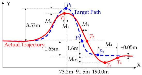
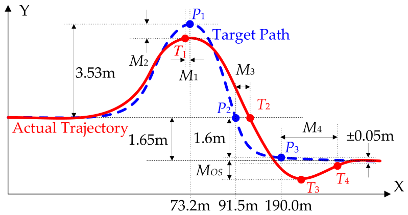
Figure 3 illustrates the target path and performance measures used to assess path-tracking performance. Based on the points P₁–P₃ on the reference path and T₁–T₄ on the trajectory, five indices M₁–M₄ and M_OS are defined in (37). M₁ and M₂ denote the longitudinal and lateral peak offsets, respectively, whereas M₃ and M₄ represent the response and settling delays, respectively. M_OS represents the percentage overshoot. As defined in (37), the terms x(★) and y(★) refer to the horizontal and vertical coordinates of point ★, in that order. Smaller values generally indicate better path-tracking performance, except for M₂ and M_OS. The smaller |M_OS|, the better; and the larger M₂, the better.

$$\left\{\begin{array}{l}{M}_1=x\left(T_1\right)-x\left(P_1\right)=x\left(T_1\right)-73.2\\ M_2=y\left(T_1\right)-y\left(P_1\right)=y\left(T_1\right)-3.53\\ M_3=x\left(T_2\right)-x\left(P_2\right)=x\left(T_2\right)-91.5\\ M_4=x\left(T_4\right)-x\left(P_3\right)=x\left(T_4\right)-190.0\\ M_{OS}={\displaystyle \frac{\left|y\left(T_3\right)-1.65\right|}{1.65+3.53}}\times 100\end{array}\right.$$

(37)

Figure 3. Target path and performance measures used to assess path-tracking performance.

In Figure 3, M₁ and M₂ stand for the responsiveness and target-reaching capability of the controller, respectively. The path-tracking performance is regarded as satisfactory when M₂ > −0.05 m. M_OS denotes the lateral damping capability and serves as an agility index. The performance is considered acceptable when M_OS < 16%. M₃ denotes the response delay, whereas M₄ is defined as the settling distance needed for the vehicle trajectory to reach convergence at the target position T₄. Hence, M₄ represents the rate at which the lateral motion converges to y = −1.65 m. On low-friction surfaces, satisfactory performance is achieved when M₄ < 16 m. The best performance is generally obtained when M_OS is approximately 1% with M₂ > −0.05 m. Accordingly, the weighting parameters and k_v are selected to maintain M₂ ≈ −0.02 m, for which M_OS remains below 1%. Further details are given in [17,29,31,32].

Lateral stability is commonly evaluated using β. In practice, stability is considered acceptable when |β| < 3° [29]. Smaller values of β indicate better stability. In this paper, the maximum absolute β and the maximum absolute rate of β are defined as MASA and MASR, respectively.

4. Simulation and Discussion

The five controllers considered in this study, namely LQR4, LQR3, LQR2, LQSOF3, and LQSOF2, were implemented in Simulink of MATLAB 2024a and tested in conjunction with CarSim 8.0 through co-simulation [44]. The simulation framework was configured to compare the controllers under identical maneuver and road conditions so that their path-tracking characteristics could be examined on a common basis. The simulation scenario is given in Figure 3. The test vehicle in CarSim was an F-segment sedan model [17,36,37,38]. The vehicle model parameters and corresponding values for the CarSim F-segment sedan are summarized in Table 1.

Table 1. Vehicle model parameters and corresponding values for the CarSim F-segment sedan.

Parameters	Values	Parameters	Values
m	1823 kg	Iz	6286 kg-m2
lf	1.265 m	lr	1.900 m
Cf	43,000 N/rad	Cr	63,000 N/rad

The vehicle was assumed to employ either an FWS or a 4WS system, both modeled as first-order actuators with a bandwidth of 5 Hz. Throughout the simulations, the longitudinal velocity v_x was maintained at 60 km/h using the built-in speed controller in CarSim, so that uncertainty associated with v_x was minimized. Simulations were conducted under two road conditions, with friction coefficients of 0.85 and 0.4 for the high- and low-friction surfaces, respectively. The total simulation time for each run was 10 s.

Low-speed cases were not considered because path-tracking performance generally improves as the vehicle speed decreases. To better distinguish controller performance, simulations were conducted under high-speed and low-friction conditions. Under low-speed or high-friction conditions, most path-tracking controllers exhibit similarly good performance.

In practical implementation, the evaluation of e_y, e_y,p and e_ψ requires localization and motion-sensing information from GNSS/GPS, an IMU, cameras, and wheel-speed sensors. GNSS/GPS provides global position information, whereas the IMU and wheel-speed sensors improve short-term motion estimation and compensate for GNSS degradation. When the target path is defined as the lane center, camera-based perception and computer-vision algorithms are additionally required, which may increase the computational burden. These implementation issues are discussed in detail in the survey papers [1,2,3,4,5].

When implementing LQR4, measurement or estimation of β is also required. Because direct measurement of β generally requires expensive sensing equipment, a state estimator is needed. For this purpose, an extended Kalman filter was designed and applied in this study [40].

4.1. Simulation on High-Friction Surface

The first set of simulations was carried out on the high-friction surface where μ = 0.85. For this case, the preview gain k_v was chosen as 0.14, and the weighting matrices in J₄, J₃ and J₂ were adjusted so that M₂ remained close to −0.02 m while MASA was kept below 2°. The preview gain and the admissible upper bounds in LQOF are presented in Appendix A. As a result, the differences in some measures, M₂ and M_OS, became small, allowing the comparison to focus more clearly on transient responsiveness and convergence behavior. In other words, the main discriminating metrics became M₁, M₃, and M₄, with MASA used as a stability constraint rather than a dominant performance separator.

Table 2 and Table 3 show a comparison of LQR and LQ SOF controller responses with FWS and 4WS on the high-friction surface, in that order. Based on the results summarized in Table 2 and Table 3, the controllers may be divided into two distinct sets, namely LQR4/LQR3/LQSOF3 and LQR2/LQSOF2. Let these two groups be denoted as LQFC43 and LQFC2, respectively.

Table 2. Comparison of LQR and LQ SOF controller responses with FWS on the high-friction surface.

Controllers	M1 (m)	M2 (m)	MOS (%)	M3 (m)	M4 (m)	MASA (Deg)	MASR (Deg/s)
LQR4	−0.05	−0.02	0.0	0.26	1.21	1.1	6.2
LQR3	−0.06	−0.02	0.0	0.25	1.40	1.1	6.1
LQR2	−0.30	−0.02	0.0	−0.19	1.12	1.2	8.8
LQSOF3	0.06	−0.02	0.0	0.25	0.17	1.1	5.8
LQSOF2	−0.47	−0.02	0.0	−0.23	3.10	1.1	7.9

Table 3. Comparison of LQR and LQ SOF controller responses with 4WS on the high-friction surface.

Controllers	M1 (m)	M2 (m)	MOS (%)	M3 (m)	M4 (m)	MASA (Deg)	MASR (Deg/s)
LQR4	−0.16	−0.02	0.00	0.10	2.92	1.1	5.8
LQR3	−0.08	−0.02	−0.01	0.21	1.07	1.1	6.3
LQR2	−0.30	−0.02	−0.00	−0.15	1.34	1.1	8.0
LQSOF3	−0.01	−0.02	−0.00	0.09	1.16	1.1	5.1
LQSOF2	−0.28	−0.02	−0.00	−0.14	1.57	1.1	7.4

As shown in Table 2, LQR2 and LQSOF2 with FWS using (e_y,p, e_ψ) show faster responses than the others in terms of M₁. However, LQSOF2 shows the slowest convergence in terms of M₄. In contrast, LQSOF3 shows the fastest convergence among these controllers. No significant differences are observed in the remaining performance measures among these controllers. Table 3 indicates that, with 4WS, LQR2 and LQSOF2 provide a more rapid response according to M₁, whereas their convergence to the final state is slower according to M₄. In contrast, LQR4 shows the slowest convergence among the LQR controllers. Because the DLC maneuver given in Figure 3 is designated for collision avoidance, the measures M₁ and M₂ are the most important. For this reason, it is recommended to use LQR2 with FWS on high-friction surfaces. As the next better option in view of collision avoidance, LQSOF2 provides relatively good performance with FWS and 4WS on high-friction surfaces.

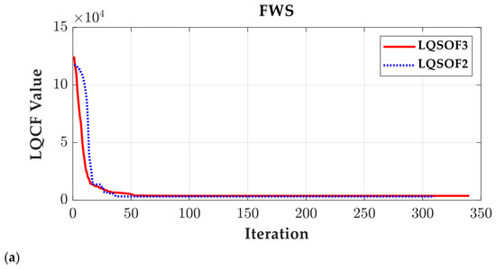
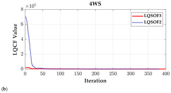
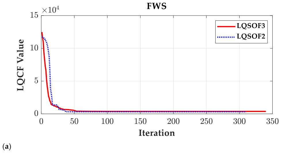
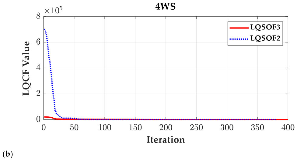
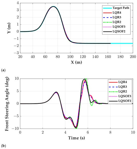
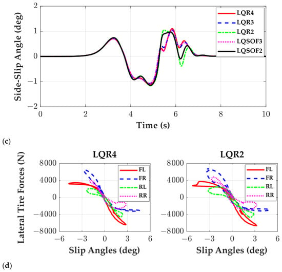
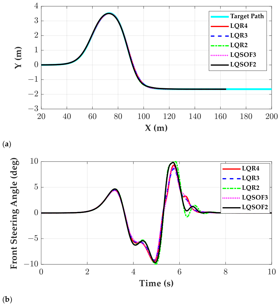
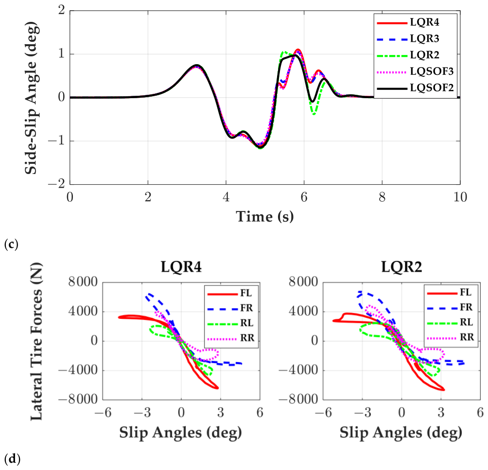
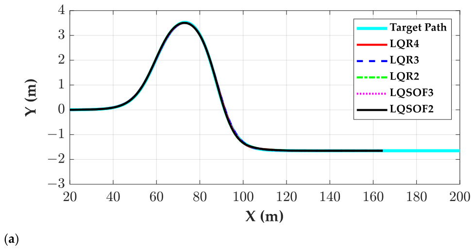
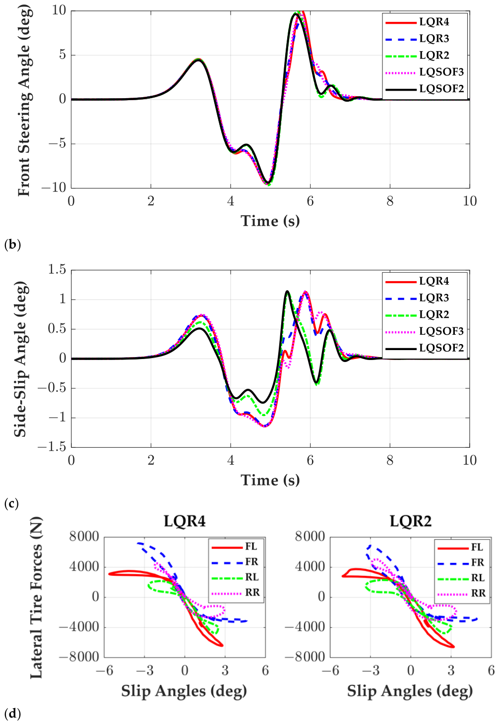
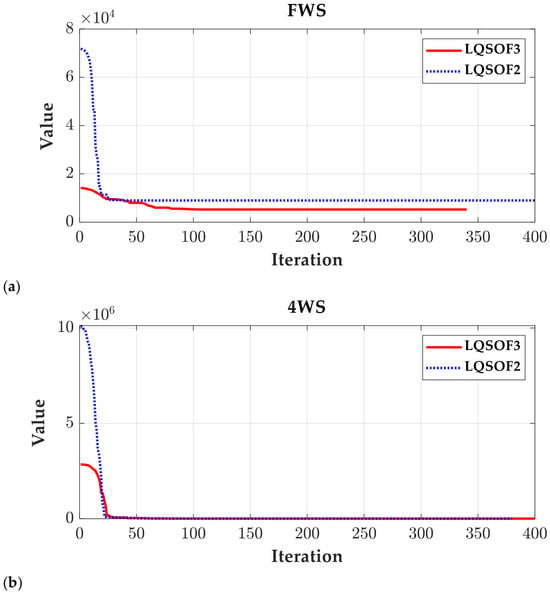
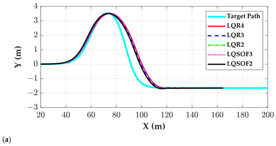
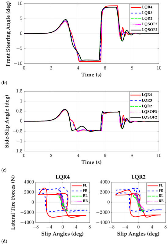
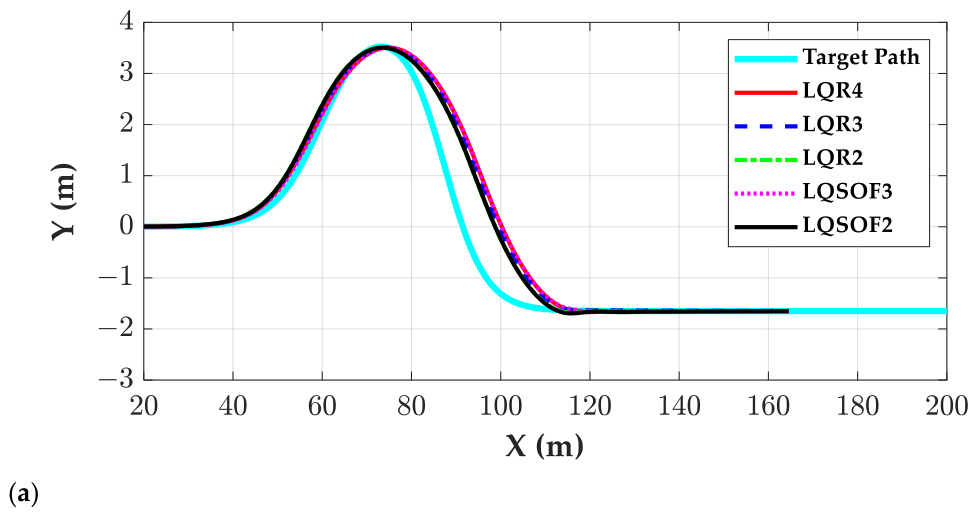
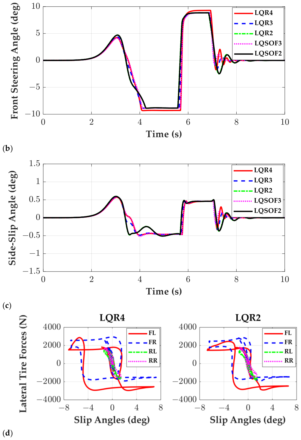
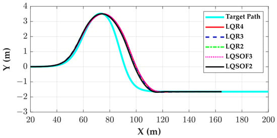
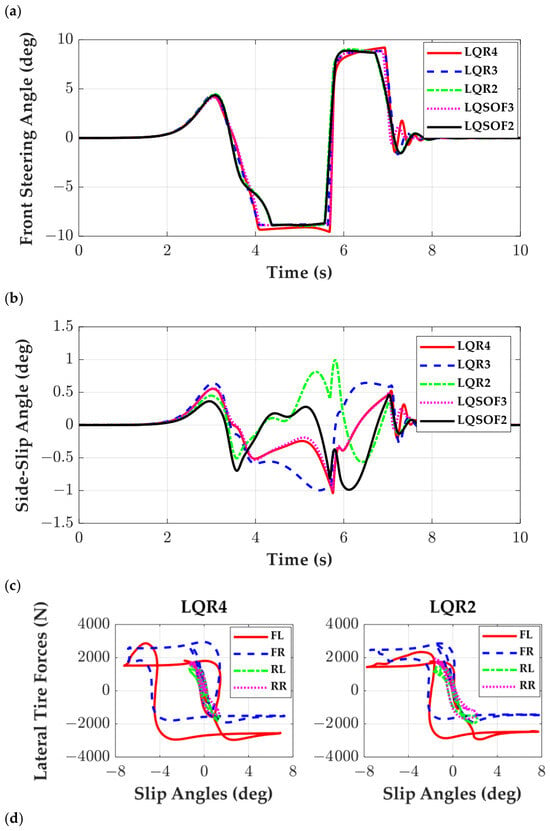
Figure 4 shows the convergence curves of CMA-ES for LQSOF3 and LQSOF2 with FWS and 4WS, in that order. As shown in these figures, CMA-ES converged in early steps. Figure 5 and Figure 6 show the trajectories, front steering angles, side-slip angles and lateral tire forces of these controllers. As illustrated in these figures, there are only slight differences among the controllers under both FWS and 4WS, except for the side-slip-angle responses in the 4WS case. As illustrated in Figure 6c, the controllers in LQFC43, i.e., LQR4, LQR3 and LQSOF3, show similar side-slip angles. On the other hand, the controllers in LQFC2, i.e., LQR2 and LQSOF2, show similar trends. This is attributed to the fact that both LQR2 and LQSOF2 use two state variables, e_y,p and e_ψ, for path-tracking control.

Figure 4. Convergence curves of CMA-ES for LQSOF3 and LQSOF2 on the high-friction surface: (a) FWS; (b) 4WS.

Figure 5. Performance comparison of the LQR- and LQ SOF-based controllers with FWS on a high-adhesion surface: (a) vehicle trajectories; (b) front steering angles; (c) side-slip angles; (d) variation in lateral tire force with slip angle.

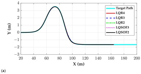
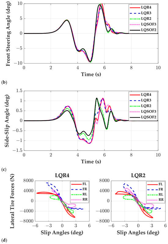
Figure 6. Performance comparison of the LQR- and LQ SOF-based controllers under 4WS on a high-adhesion surface: (a) vehicle trajectories; (b) front steering angles; (c) side-slip angles; (d) variation in lateral tire force with slip angle.

As illustrated in Figure 5a–c and Figure 6a–c, only slight differences are observed among the controllers with regard to the vehicle trajectory, front steering angle, and side-slip angle. As illustrated in Figure 5d and Figure 6d, the lateral tire forces of the controllers in the LQFC43 are similar to one another, and those of the controllers in the LQFC2 are similar to each other. For this reason, the lateral tire forces of LQR4 and LQR2 are drawn as representatives. As observed in these figures, LQR2 generates greater lateral tire forces than LQR4 because it produces larger tire slip angles. These differences generated a performance difference between LQFC43 and LQFC2.

In the DLC maneuver at 60 km/h, LQR2 and LQSOF2 exhibited faster transient response with competitive overall performance. This suggests that they use only e_y,p and e_ψ, which are the most dominant variables for aggressive path correction. Owing to this simplified feedback structure, the steering action is more directly focused on reducing path-tracking errors, thereby producing a faster lateral response and more effective lateral tire force generation. This can be identified in Figure 5b,c and Figure 6b,c. In contrast, LQR4 and LQR3 additionally reflect the internal vehicle states, such as β and γ, so part of their control effort is devoted to regulating lateral-yaw dynamics, which tends to make the steering action relatively more conservative.

4.2. Simulation on Low-Friction Surface

The second set of simulations was carried out on the low-friction surface where μ = 0.4. For this case, the preview gain k_v was chosen as 0.245, and the weighting matrices in J₄, J₃ and J₂ were adjusted so that M₂ remained close to −0.02 m while MASA was kept below 1°. This allowed the comparison to focus on how the controller structure influences responsiveness and convergence under more stability-critical conditions. Moreover, the main discriminating metrics became M₁, M₃, and M₄, with MASA used as a stability constraint rather than a dominant performance separator. The preview gain and the admissible upper bounds in LQOF are presented in Appendix A.

Table 4 and Table 5 show a comparison of LQR and LQ SOF controller responses with FWS and 4WS on the low-friction surface, in that order. According to Table 4 and Table 5, the LQFC2 group, consisting of LQR2 and LQSOF2, yields smaller M₁ and M₄ values than the other controllers, indicating faster response and convergence speeds. In particular, LQR2 shows better performance with FWS and 4WS on high- and low-friction surfaces. This trend is consistent with that observed on the high-friction surface. This result is somewhat unexpected because SSM2 does not include explicit tire-force terms; in other words, it is essentially a kinematic model. Under the present tuning and maneuver conditions, the controllers based on reduced-order models exhibited superior transient path-tracking performance despite their simpler structure. From the overall trends in Table 4 and Table 5, it can be inferred that 4WS generally improves convergence, as reflected by the smaller M₄ values, although this benefit is accompanied by an increase in β.

Table 4. Comparison of LQR and LQ SOF controller responses with FWS on the low-friction surface.

Controllers	M1 (m)	M2 (m)	MOS (%)	M3 (m)	M4 (m)	MASA (Deg)	MASR (Deg/s)
LQR4	1.68	−0.02	0.4	8.70	5.43	0.6	13.1
LQR3	1.12	−0.02	0.0	8.04	5.10	0.6	12.7
LQR2	0.29	−0.02	0.5	7.20	2.98	0.6	11.7
LQSOF3	1.78	−0.02	0.1	8.71	6.14	0.6	13.2
LQSOF2	0.36	−0.02	0.9	7.24	2.67	0.6	11.7

Table 5. Comparison of LQR and LQ SOF controller responses with 4WS on the low-friction surface.

Controllers	M1 (m)	M2 (m)	MOS (%)	M3 (m)	M4 (m)	MASA (Deg)	MASR (Deg/s)
LQR4	1.69	−0.02	0.5	8.52	4.81	1.0	11.2
LQR3	1.12	−0.02	0.7	7.96	3.67	1.0	13.5
LQR2	0.68	−0.02	0.7	7.46	2.75	1.0	8.4
LQSOF3	1.83	−0.02	0.0	8.57	5.95	1.0	11.2
LQSOF2	0.71	−0.02	0.7	7.26	2.76	1.0	6.9

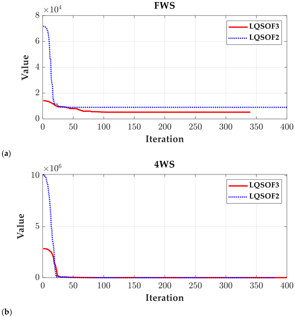
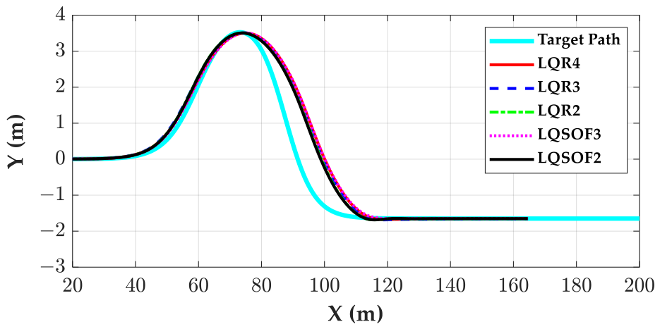
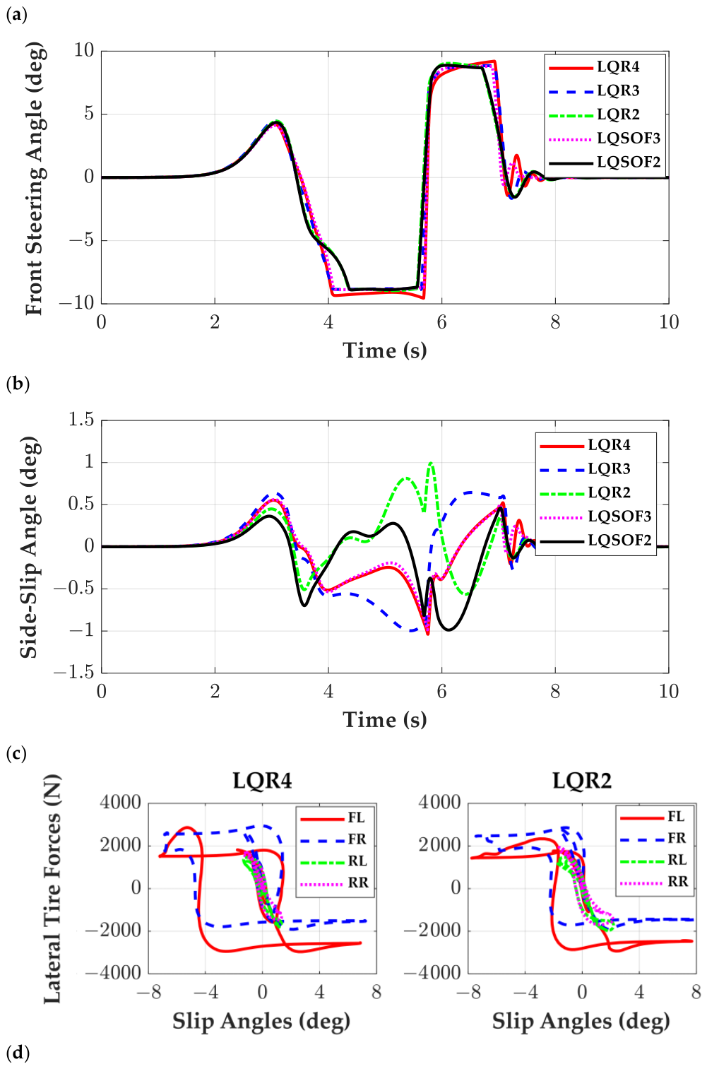
Figure 7 shows the CMA-ES convergence curves for LQSOF3 and LQSOF2 under the FWS and 4WS configurations. As shown in Figure 7, CMA-ES converged within the early iterations. This behavior is consistent with that observed in Figure 4. Figure 8 and Figure 9 present the trajectories, front steering angles, side-slip angles, and lateral tire forces produced by these controllers. As shown in Figure 8 and Figure 9, only slight differences are observed among the controllers with both FWS and 4WS systems, except for β responses in the 4WS case. These results indicate that the use of 4WS leads to an increase in β. Unlike the results on the high-friction surface, the MASA values are below 1° because of the low-friction condition. As shown in Figure 8c and Figure 9c, the counter-steering action around 3.5 s is fastest for LQR2 and LQSOF2. As a result, the values of M₁ for LQR2 and LQSOF2 are the smallest. As shown in Figure 8d and Figure 9d, the lateral tire forces of LQR4 and LQR2 show the same trend as on the high-friction surface.

Figure 7. Convergence curves of CMA-ES for LQSOF3 and LQSOF2 on the low-friction surface: (a) FWS; (b) 4WS.

Figure 8. Performance comparison of the LQR- and LQ SOF-based controllers under FWS on a low-adhesion surface: (a) vehicle trajectories; (b) front steering angles; (c) side-slip angles; (d) variation in lateral tire force with slip angle.

Figure 9. Performance comparison of the LQR- and LQ SOF-based controllers under 4WS on a low-adhesion surface: (a) vehicle trajectories; (b) front steering angles; (c) side-slip angles; (d) variation in lateral tire force with slip angle.

From the simulation results on high and low friction surfaces, LQR2, designed with SSM2, appears to be the most favorable option among the tested controllers on the low-friction surface for a severe DLC maneuver, regardless of the selected actuator.

4.3. Robustness and Parameter Sensitivity Evaluation Based on Full-Factorial Analysis

The third set of simulations was carried out for robustness and parameter sensitivity analysis. The parameters, which were assumed to be uncertain in this paper, are m_s, I_z, μ, v_x and k_v. Among the parameters, m_s and I_z were grouped into a single parameter, (m_s, I_z), because I_z is proportional to m_s. The uncertainties of C_f and C_r are assumed to be identical to that of μ because those parameters are proportional to μ. In this paper, 10% of parameter variation was assumed. As a result, the ranges of variations in those parameters are given in Table 6. In Table 6, F1~F4 corresponds to (m_s, I_z), μ, v_x and k_v, and two levels, L1 and L2, represent the lower and upper bounds, obtained from 10% perturbation. Using the nominal parameter set listed in Table 6, the controllers were adjusted so that M₂ remained close to −0.02 m. As a result, the fixed gain for each controller was obtained and used for robustness and sensitivity analyses.

Table 6. Ranges of variation in each parameter/factor.

Factors	Parameters	Nominal	Level1 (L1)	Level2 (L2)
F1	(ms, Iz)	(1823, 6286)	(1732, 5972)	(1914, 6600)
F2	μ	0.6	0.5	0.7
F3	vx	40 km/h	30 km/h	50 km/h
F4	kv	0.140	0.126	0.154

In the robustness and sensitivity analysis, the uncertainty factors were limited to (m_s, I_z), μ, v_x and k_v. This choice was made because, within the adopted linear tire modeling framework, variation in the road friction coefficient represents the dominant uncertainty affecting lateral tire-force generation, so that an additional variation in tire cornering stiffness would provide largely overlapping information. In contrast, actuator bandwidth mainly acts as a common hardware limitation that delays steering response and degrades transient performance in a qualitatively similar manner for all controllers, rather than serving as a controller-discriminating design parameter. Therefore, the present study focuses on the uncertainty factors that are more directly related to the vehicle model and the comparative characteristics of the controllers.

Since the four parameters given in Table 6 have lower and upper bounds, they each have two levels, i.e., L1 and L2, and, consequently, 2⁴ = 16 runs are needed for each controller. Using the level combinations defined by L1 and L2 for the parameters in Table 6, 2⁴ full-factorial simulations were conducted. From the simulations, M₁, M₂, M_OS, M₃, M₄ and β were obtained. Using these simulation results, robustness and parameter sensitivity were analyzed.

Since only one response value was available for each factor combination, the robustness comparison was not based on significance-oriented ANOVA, but on an effect-size-oriented variability assessment. In the analysis, the response variables were M₁, M₂, M_OS, M₃, M₄, and β. Since M₁, M_OS, M₃, M₄, and β are smaller-the-better responses, whereas M₂ is larger-the-better, M₂ was converted into a loss-type response so that all responses could be assessed on a common smaller-is-better basis. Since the desirable value of M_OS is close to zero regardless of sign, M_OS was converted into an absolute-value-type response, i.e., ∣M_OS∣, so that smaller values indicate better performance.

For each controller and response, the standard deviation and range over the 16 factorial runs were calculated to quantify overall variability. In addition, the main effects, two-factor interaction effects, and all factorial effects were calculated using coded factor levels (−1, +1), and their absolute magnitudes were used as sensitivity measures. The robustness indices of each controller were then obtained by averaging these response-level quantities over the six responses. Finally, inverse min-max normalization was applied to convert each index into a 0–100 score, and the overall robustness score was defined as the average of the five component scores corresponding to the standard deviation, range, main effects, two-factor interactions, and total factorial effects. A higher robustness score indicates that the controller is less sensitive to factor variations over the full factorial space.

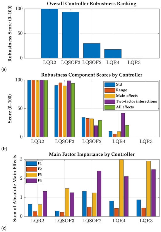
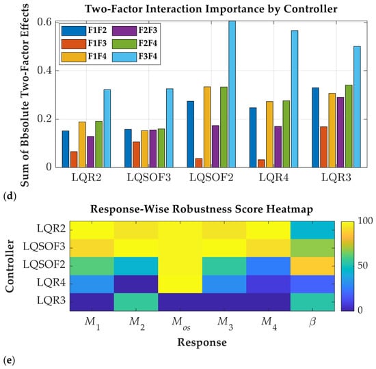
Figure 10 shows the robustness comparison results of the five controllers with FWS based on the 2⁴ full-factorial simulations. Figure 10a,b show that LQR2 achieved the highest overall robustness, followed by LQSOF3, whereas LQR3 exhibited the lowest robustness among the five controllers. This ranking was consistently supported by the smaller averaged variability and factorial-effect magnitudes of LQR2 and LQSOF3. In the response-wise comparison as shown in Figure 10e, LQR2 was particularly robust in M₁ and M₄, whereas LQSOF3 showed the most stable behavior in M₂ and M₃. Although LQSOF2 yielded favorable robustness in β, its overall robustness remained lower than that of LQR2 and LQSOF3 when all responses were considered together. The factor-importance analysis indicated that the dominant main factor was F4(k_v) for LQR2 and LQSOF2, but F3(v_x) for LQR3, LQR4, and LQSOF3, as shown in Figure 10c. Moreover, as shown in Figure 10d, the most influential two-factor interaction was consistently F3 × F4 for all controllers, implying that the coupled variation in these two factors is the primary source of robustness degradation.

Figure 10. Robustness comparison of the five controllers with FWS based on the 2⁴ full-factorial simulation: (a) overall robustness score; (b) component-wise robustness scores; (c) main-factor importance; (d) two-factor interaction importance; (e) response-wise robustness score heatmap. Higher scores indicate better robustness, whereas larger factor-importance values indicate greater sensitivity to the corresponding factor variations.

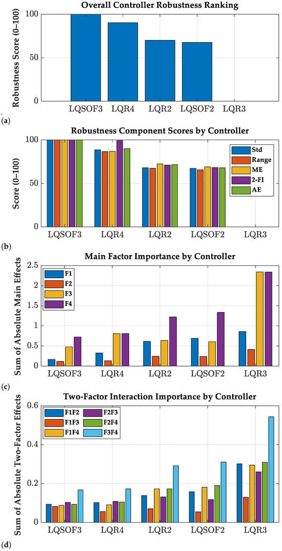
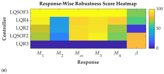
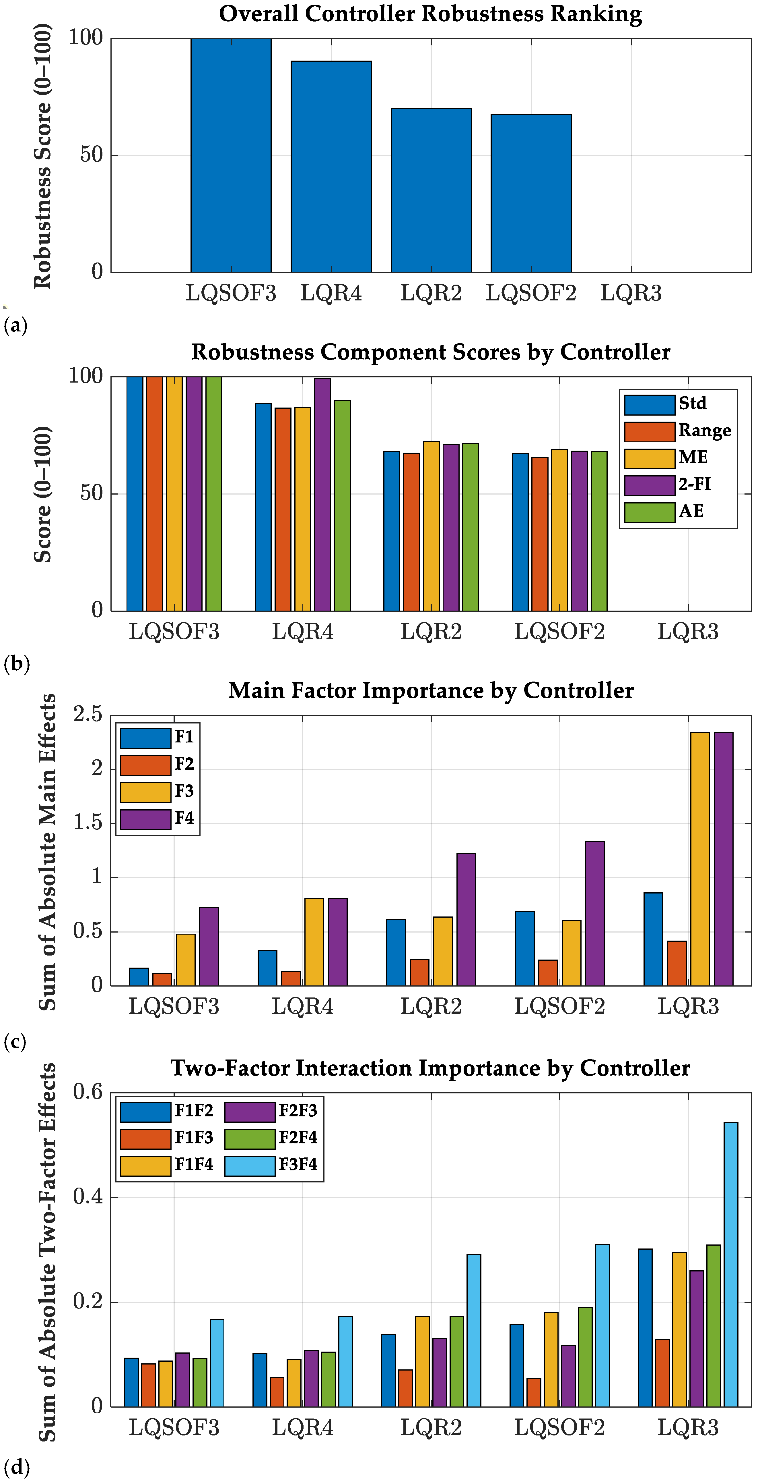
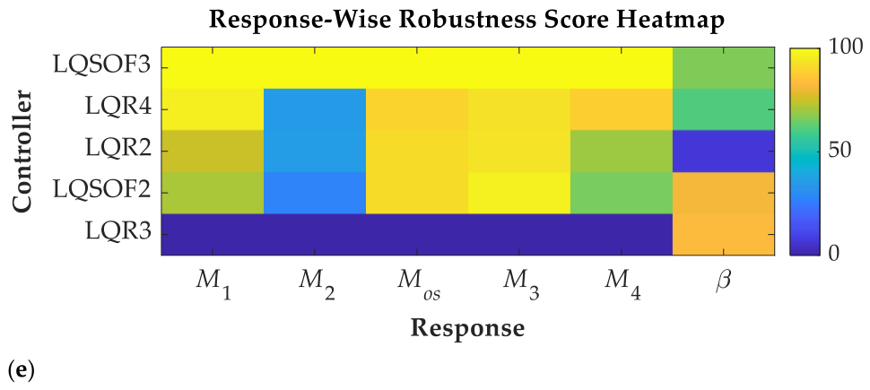
Figure 11 shows the robustness comparison results of the five controllers with 4WS based on the 2⁴ full-factorial simulations. Figure 11a shows that LQSOF3 achieved the highest overall robustness, followed by LQR4, whereas LQR3 was the most sensitive to factor variations. This ranking was consistently supported by the smaller averaged standard deviation, response range, and factorial-effect magnitudes of LQSOF3 and LQR4. In the response-wise comparison, as shown in Figure 11e, LQSOF3 provided the most robust behavior in M₁, M₂, M_OS, M₃ and M₄, indicating that its performance remained the most stable over the factorial domain. Although LQR3 showed the best robustness in β, its overall robustness was the poorest because it exhibited much larger variability and larger factorial sensitivities in most of the other response variables. The factor-importance analysis given in Figure 11c further revealed that F4 was the dominant main factor for most controllers. This means that F4(k_v) is critical in path tracking with 4WS on a low-friction surface [29,30]. As shown in Figure 11d, the most influential two-factor interaction was consistently F3 × F4. These results suggest that the superior robustness of LQSOF3 arises from its reduced sensitivity not only to individual factor changes but also to the coupled perturbation associated with F3 × F4.

Figure 11. Robustness comparison of the five controllers with 4WS based on the 2⁴ full-factorial simulation: (a) overall robustness score; (b) component-wise robustness scores; (c) main-factor importance; (d) two-factor interaction importance; (e) response-wise robustness score heatmap. Higher scores indicate better robustness, whereas larger factor-importance values indicate greater sensitivity to the corresponding factor variations.

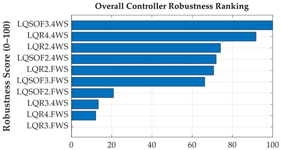
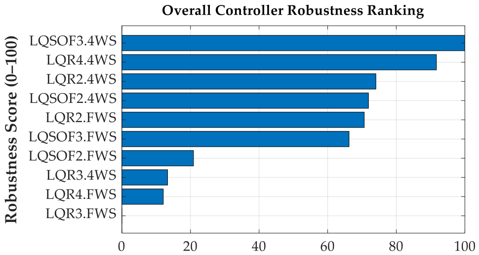
To compare the two actuator configurations, namely FWS and 4WS, the two full-factorial simulation datasets described above were combined and the robustness ranking was obtained for the ten controllers with FWS and 4WS. Figure 12 shows the overall robustness ranking of the ten controllers with FWS and 4WS, based on the 2⁴ full-factorial simulations.

Figure 12. Overall controller robustness ranking of the ten controllers with FWS and 4WS. Higher scores indicate better robustness against factor variations.

The ranking given in Figure 12 indicates that the 4WS configurations are consistently less sensitive to factor variations than the FWS counterparts. As shown in Figure 12, the most robust controller was LQSOF3.4WS, followed by LQR4.4WS, LQR2.4WS, and LQSOF2.4WS. In contrast, the FWS controllers generally exhibited larger dispersion and stronger factor dependence, with LQR3.FWS and LQR4.FWS showing the poorest robustness. These results suggest that the additional rear-wheel steering action effectively reduces the sensitivity of path-tracking performance to parameter variations and operating-condition changes, thereby improving the overall robustness of the closed-loop system.

5. Conclusions

This study provides a comparative evaluation of path-tracking controllers designed with state-space models of different orders. A four-state model is derived from the target path and the bicycle model, and three-state and two-state reduced models are obtained under simplifying assumptions. Based on the four-state model, two LQ static output-feedback (SOF) controllers are designed. The path-tracking capabilities of the controllers were assessed by means of simulations carried out with the CarSim vehicle dynamics software. Moreover, the robustness and parameter sensitivity analyses were conducted on the controllers. In summary, the goal of this paper is the systematic comparison of two different controller simplification strategies, namely model-order reduction and output-feedback reduction, and the provision of practical insight into their performance–complexity trade-off for path tracking.

From the simulation results, several observations can be drawn:

• On high-friction and low-friction surfaces, LQR2 with FWS and 4WS provides favorable path-tracking performance. LQR2 was designed with SSM2, which is derived from a kinematic model. This is contrary to the conventional belief that the larger the number of state variables, the better the performance. From this result, LQR2 is recommended for severe DLC maneuvers regardless of the selected actuator and road friction condition.
• The controllers using two state variables, i.e., LQR2 and LQSOF2, provide better performance than those using three or four state variables, i.e., LQR4, LQR3 and LQSOF3. This behavior can be attributed to the use of only the lateral offset and heading errors in LQR2 and LQSOF2, which constitute the primary states governing aggressive path-following correction.
• Using 2⁴ full-factorial simulations, robustness and parameter-sensitivity analyses were conducted for the ten controllers. These analyses showed that LQR2 and LQSOF3 were the most robust controllers for FWS and 4WS, respectively, and that most controllers with 4WS, except LQR3, were more robust than their FWS counterparts. It was also found that the single parameter v_x or k_v and their interaction v_x × k_v have the greatest influence on the path-tracking performance.

This study examined how model order influences the control performance of path-tracking systems. The results indicate that a model based only on lateral offset error and heading error can provide better performance under the tested conditions. Since SSM3 and SSM2 are control-oriented reduced models derived under simplifying assumptions, the present conclusions are limited to the operating conditions examined in this study. Therefore, the results should be interpreted as comparative findings under the tested DLC scenarios, rather than as universal conclusions over all speeds, curvatures, friction levels, and parameter uncertainties. Broader robustness validation is left for future work. Furthermore, motivated by these results, future work will extend the state-space formulation and performance validation to the pure pursuit and Stanley methods, which are widely used in autonomous-vehicle path tracking.

References

- Montanaro, U.; Dixit, S.; Fallaha, S.; Dianatib, M.; Stevensc, A.; Oxtobyd, D.; Mouzakitisd, A. Towards connected autonomous driving: Review of use-cases. Veh. Syst. Dyn. 2019, 57, 779–814. [Google Scholar] [CrossRef] [Scilit]
- Yurtsever, E.; Lambert, J.; Carballo, A.; Takeda, K. A survey of autonomous driving: Common practices and emerging technologies. IEEE Access 2020, 8, 58443–58469. [Google Scholar] [CrossRef] [Scilit]
- Omeiza, D.; Webb, H.; Jirotka, M.; Kunze, M. Explanations in autonomous driving: A survey. IEEE Trans. Intell. Transp. Syst. 2022, 23, 10142–10162. [Google Scholar] [CrossRef] [Scilit]
- Paden, B.; Cap, M.; Yong, S.Z.; Yershov, D.; Frazzoli, E. A survey of motion planning and control techniques for self-driving urban vehicles. IEEE Trans. Intell. Veh. 2016, 1, 33–55. [Google Scholar] [CrossRef] [Scilit]
- Sorniotti, A.; Barber, P.; De Pinto, S. Path tracking for automated driving: A tutorial on control system formulations and ongoing research. In Automated Driving; Watzenig, D., Horn, M., Eds.; Springer: Cham, Switzerland, 2017. [Google Scholar]
- Amer, N.H.; Hudha, H.Z.K.; Kadir, Z.A. Modelling and control strategies in path tracking control for autonomous ground vehicles: A review of state of the art and challenges. J. Intell. Robot. Syst. 2017, 86, 225–254. [Google Scholar] [CrossRef] [Scilit]
- Bai, G.; Meng, Y.; Liu, L.; Luo, W.; Gu, Q.; Liu, L. Review and comparison of path tracking based on model predictive control. Electronics 2019, 8, 1077. [Google Scholar] [CrossRef] [Scilit]
- Yao, Q.; Tian, Y.; Wang, Q.; Wang, S. Control strategies on path tracking for autonomous vehicle: State of the art and future challenges. IEEE Access 2020, 8, 161211–161222. [Google Scholar] [CrossRef] [Scilit]
- Rokonuzzaman, M.; Mohajer, N.; Nahavandi, S.; Mohamed, S. Review and performance evaluation of path tracking controllers of autonomous vehicles. IET Intell. Transp. Syst. 2021, 15, 646–670. [Google Scholar] [CrossRef] [Scilit]
- Stano, P.; Montanaro, U.; Tavernini, D.; Tufo, M.; Fiengo, G.; Novella, L.; Sorniotti, A. Model predictive path tracking control for automated road vehicles: A review. Annu. Rev. Control 2022, 55, 194–236. [Google Scholar] [CrossRef] [Scilit]
- Yakub, F.; Mori, Y. Comparative study of autonomous path-following vehicle control via model predictive control and linear quadratic control. Proc. Inst. Mech. Eng. Part D J. Automob. Eng. 2015, 229, 1695–1714. [Google Scholar] [CrossRef] [Scilit]
- Wang, R.; Yin, G.; Zhuang, J.; Zhang, N.; Chen, J. The path tracking of four-wheel steering autonomous vehicles via sliding mode control. In Proceedings of the 2016 IEEE Vehicle Power and Propulsion Conference (VPPC), Hangzhou, China, 17–20 October 2016. [Google Scholar]
- Lee, K.; Jeon, S.; Kim, H.; Kum, D. Optimal path tracking control of autonomous vehicle: Adaptive full-state linear quadratic gaussian (LQG) control. IEEE Access 2019, 7, 109120–109133. [Google Scholar] [CrossRef] [Scilit]
- Hang, P.; Chen, X. Path tracking control of 4-wheel steering autonomous ground vehicles based on linear parameter-varying system with experimental verification. Proc. Inst. Mech. Eng. Part I J. Syst. Control Eng. 2021, 235, 411–423. [Google Scholar] [CrossRef] [Scilit]
- Barari, A.; Afshari, S.S.; Liang, X. Coordinated control for path-following of an autonomous four in-wheel motor drive electric vehicle. Proc. Inst. Mech. Eng. Part C J. Mech. Eng. Sci. 2022, 236, 6335–6346. [Google Scholar] [CrossRef] [Scilit]
- Du, Q.; Zhu, C.; Li, Q.; Tian, B.; Li, L. Optimal path tracking control for intelligent four-wheel steering vehicles based on MPC and state estimation. Proc. Inst. Mech. Eng. Part D J. Automob. Eng. 2022, 236, 1964–1976. [Google Scholar] [CrossRef] [Scilit]
- Lee, J.; Yim, S. Comparative study of path tracking controllers on low friction roads for autonomous vehicles. Machines 2023, 11, 403. [Google Scholar] [CrossRef] [Scilit]
- Guo, J.; Luo, Y.; Li, K.; Dai, Y. Coordinated path-following and direct yaw-moment control of autonomous electric vehicles with sideslip angle estimation. Mech. Syst. Signal Process. 2018, 105, 183–199. [Google Scholar] [CrossRef] [Scilit]
- Chen, X.; Peng, Y.; Hang, P.; Tang, T. Path tracking control of four-wheel independent steering electric vehicles based on optimal control. In Proceedings of the 2020 39th Chinese Control Conference (CCC), Shenyang, China, 27–30, July 2020; IEEE: New York, NY, USA, 2020; pp. 5436–5442. [Google Scholar]
- Wu, H.; Si, Z.; Li, Z. Trajectory tracking control for four-wheel independent drive intelligent vehicle based on model predictive control. IEEE Access 2020, 8, 73071–73081. [Google Scholar] [CrossRef] [Scilit]
- Peng, H.; Wang, W.; An, Q.; Xiang, C.; Li, L. Path tracking and direct yaw moment coordinated control based on robust MPC with the finite time horizon for autonomous independent-drive vehicles. IEEE Trans. Veh. Technol. 2020, 69, 6053–6066. [Google Scholar] [CrossRef] [Scilit]
- Xiang, C.; Peng, H.; Wang, W.; Li, L.; An, Q.; Cheng, S. Path tracking coordinated control strategy for autonomous four in-wheel-motor independent-drive vehicles with consideration of lateral stability. Proc. Inst. Mech. Eng. Part D J. Automob. Eng. 2021, 235, 1023–1036. [Google Scholar] [CrossRef] [Scilit]
- Yang, K.; Tang, X.; Qin, Y.; Huang, Y.; Wang, H.; Pu, H. Comparative study of trajectory tracking control for automated vehicles via model predictive control and robust H-infinity state feedback control. Chin. J. Mech. Eng. 2021, 34, 74. [Google Scholar] [CrossRef] [Scilit]
- Wang, G.; Liu, L.; Meng, Y.; Gu, Q.; Bai, G. Integrated path tracking control of steering and braking based on holistic MPC. IFAC PapersOnLine 2021, 54, 45–50. [Google Scholar] [CrossRef] [Scilit]
- Xie, J.; Xu, X.; Wang, F.; Tang, Z.; Chen, L. Coordinated control based path following of distributed drive autonomous electric vehicles with yaw-moment control. Control Eng. Pract. 2021, 106, 104659. [Google Scholar] [CrossRef] [Scilit]
- Ahn, T.; Lee, Y.; Park, K. Design of integrated autonomous driving control system that incorporates chassis controllers for improving path tracking performance and vehicle stability. Electronics 2021, 10, 144. [Google Scholar] [CrossRef] [Scilit]
- Wang, G.; Liu, L.; Meng, Y.; Gu, Q.; Bai, G. Integrated path tracking control of steering and differential braking based on tire force distribution. Int. J. Control Autom. Syst. 2022, 20, 536–550. [Google Scholar] [CrossRef] [Scilit]
- Wang, W.; Zhang, Y.; Yang, C.; Qie, T.; Ma, M. Adaptive model predictive control-based path following control for four-wheel independent drive automated vehicles. IEEE Trans. Intell. Transp. Syst. 2022, 23, 14399–14412. [Google Scholar] [CrossRef] [Scilit]
- Park, M.; Yim, S. Comparative study on coordinated control of path tracking and vehicle stability for autonomous vehicles on low-friction roads. Actuators 2023, 12, 398. [Google Scholar] [CrossRef] [Scilit]
- Lee, J.; Yim, S. Path tracking control with constraint on tire slip angles under low-friction road conditions. Appl. Sci. 2024, 14, 1066. [Google Scholar] [CrossRef] [Scilit]
- Park, M.; Yim, S. Design of a path-tracking controller with an adaptive preview distance scheme for autonomous vehicles. Machines 2024, 12, 764. [Google Scholar] [CrossRef] [Scilit]
- Park, M.; Yim, S. Design of static output feedback integrated path tracking controller for autonomous vehicles. Processes 2025, 13, 1335. [Google Scholar] [CrossRef] [Scilit]
- Hu, C.; Jing, H.; Wang, R.; Yan, F.; Chadli, M. Robust H∞ output-feedback control for path following of autonomous ground vehicles. Mech. Syst. Signal Process. 2016, 70–71, 414–427. [Google Scholar] [CrossRef] [Scilit]
- Chen, J.; Lin, C.; Chen, B. An improved path-following method for solving static output feedback control problems. Optim. Control Appl. Methods 2016, 37, 1193–1206. [Google Scholar] [CrossRef] [Scilit]
- Nguyen, A.; Sentouh, C.; Zhang, H.; Popieul, J. Fuzzy static output feedback control for path following of autonomous vehicles with transient performance improvements. IEEE Trans. Intell. Transp. Syst. 2020, 21, 3069–3079. [Google Scholar] [CrossRef] [Scilit]
- Liang, Y.; Li, Y.; Zheng, L.; Yu, Y.; Ren, Y. Yaw rate tracking-based path-following control for four-wheel independent driving and four-wheel independent steering autonomous vehicles considering the coordination with dynamics stability. Proc. Inst. Mech. Eng. Part D J. Automob. Eng. 2021, 235, 260–272. [Google Scholar] [CrossRef] [Scilit]
- Kennouche, A.; Saifia, D.; Chadli, M.; Labiod, S. Multi-objective H2/H∞ saturated non-PDC static output feedback control for path tracking of autonomous vehicle. Trans. Inst. Meas. Control 2022, 44, 2235–2247. [Google Scholar] [CrossRef] [Scilit]
- Wong, H.Y. Theory of Ground Vehicles, 3rd ed.; John Wiley and Sons, Inc.: New York, NY, USA, 2001. [Google Scholar]
- Rajamani, R. Vehicle Dynamics and Control; Springer: New York, NY, USA, 2006. [Google Scholar]
- Kim, H.H.; Ryu, J. Sideslip angle estimation considering short-duration longitudinal velocity variation. Int. J. Automot. Technol. 2011, 12, 545–553. [Google Scholar] [CrossRef] [Scilit]
- Bryson, A.E.; Ho, Y.C. Applied Optimal Control; Hemisphere: New York, NY, USA, 1975. [Google Scholar]
- Syrmos, V.L.; Abdallah, C.T.; Dorato, P.; Grigoriadis, K. Static output feedback—A survey. Automatica 1997, 33, 125–137. [Google Scholar] [CrossRef] [Scilit]
- Hansen, N.; Muller, S.D.; Koumoutsakos, P. Reducing the time complexity of the derandomized evolution strategy with covariance matrix adaptation (CMA-ES). Evol. Comput. 2003, 11, 1–18. [Google Scholar] [CrossRef] [Scilit] [PubMed]
- Mechanical Simulation Corporation. VS Browser: Reference Manual, The Graphical User Interfaces of BikeSim, CarSim, and TruckSim; Mechanical Simulation Corporation: Ann Arbor, MI, USA, 2009. [Google Scholar]
Disclaimer/Publisher’s Note: The statements, opinions and data contained in all publications are solely those of the individual author(s) and contributor(s) and not of MDPI and/or the editor(s). MDPI and/or the editor(s) disclaim responsibility for any injury to people or property resulting from any ideas, methods, instructions or products referred to in the content. |
© 2026 by the author. Licensee MDPI, Basel, Switzerland. This article is an open access article distributed under the terms and conditions of the Creative Commons Attribution (CC BY) license.