A Method for Extracting Vehicle Dangerous Omen Scenarios from the Perspective of Agile Drivers

Abstract

Collecting a large number of dangerous omen scenarios from drivers’ first-person perspective is of great significance for training and improving end-to-end autonomous driving models. In this study, we aim at capturing driver-perspective scenarios when recognizing dangerous omens. Firstly, through the design and implementation of vehicle and virtual driving experiments, the electroencephalogram, electrocardiogram and eye movement data of the subjects are collected. Statistical tests are conducted to analyze the characteristic differences among drivers across three distinct states. It also reveals that the driver can perceive and distinguish the dangerous omen clearly. Secondly, the evolution law of drivers’ perception state is analyzed to accurately judge the time period of drivers’ dangerous omen perception. Thirdly, the Hidden Markov Model is used to build the driver perception state transition model, and then the model is calibrated and verified. Finally, the model is utilized to identify drivers’ dangerous omen perception states and extract the corresponding perspective objective scenarios, which can provide sufficient samples for training end-to-end autonomous driving models. This study is of great significance to enable the capability of vehicles to recognize dangerous omens, advancing end-to-end and other high-level autonomous driving technologies and further securing vehicle safety.

1. Introduction

Drivers with excellent agile perception can not only judge and identify the current dangerous situation, but also anticipate and recognize the potential omens behind the dangerous situation in advance. If autonomous vehicles can predict and recognize potential hazards (dangerous omen) like agile drivers, it will significantly reduce the probability of accidents and even prevent them altogether. Current studies focus on hazard perception. The content mainly includes three aspects: the assessment of hazard perception ability, the influencing factors of hazard perception ability, and the biological, psychological, and physical characteristics of drivers during hazard perception, as detailed below:

(1)

The accurate and effective measurement of hazard perception ability is of great significance for evaluating drivers’ safe driving level [1,2]. Hazard perception testing has been incorporated into drivers’ license examinations in many countries. Bruce C. et al. [3] investigated the role of the Occupational Therapy Risk Propensity Test in hazard perception assessments and validated its reliability. Sun Long et al. [4] developed a hazard prediction test for China drivers, named “What Happens Next”, and evaluated its reliability and validity. Glen F.C. et al. [5] conducted simulations and designed a driver hazard perception test under varying levels of visual field loss, which can evaluate the hazard perception ability of drivers with visual field impairment and their eligibility for road driving. Malone S. et al. [6] compared the effects of traditional test tasks, language tasks and motor tasks on the measurement of drivers’ hazard perception ability. Sepulveda J.A. et al. [7] found that the fixation frequency and stability of central vision as well as the efficiency of peripheral vision in perceiving motion stimuli are key factors in affecting the drivers’ hazard perception time. Meir A. et al. [8] believed that the ability to perceive and detect danger is an ability that grows with age and experience, so they studied the hazard perception abilities of children and experienced adults when crossing the road. Mcinerney K. et al. [9] studied the neuropsychological factors related to the hazard perception ability of older drivers. Sun L. et al. [10] developed a hazard perception test for cyclists to assess their ability of perceiving dangers during cycling. Bai Jing et al. [11] proposed an automatic assessment network for drivers’ hazard perception ability in highway scenarios with icy and snowy conditions.

(2)

The main factors affecting the ability to perceive danger include age [12,13,14,15], driver characteristics [16,17,18,19,20,21] (psychological traits, differences brought about by regional culture, etc.), diseases [22,23,24,25,26,27,28], and driving environment [29,30,31]. The hazard perception ability of drivers of different ages is often different. Mirman J.H. et al. [32] studied the relationship between adolescent drivers’ ability to actually drive vehicles on the road and parental supervision of their practice. With advancing age, drivers’ driving experience becomes increasingly rich, and their hazard perception ability is often further enhanced [33]. However, as they enter the elderly stage, their ability to perceive danger begins to decline, and this decline appears to manifest only after the age of 75 [34]. In addition, other individual differences among drivers can also lead to differences in their ability to perceive danger. The main factors include their personality [35], psychological traits [36], cultural characteristics [37], attitudes, etc. Illness is also a significant factor affecting the ability to perceive danger. This is because drivers suffer certain losses, due to their own actions or after an accident, which then affects their ability to perceive danger. Current research mainly focuses on diseases such as glaucoma [23,38,39] and mild traumatic brain injury (MTBI) [25].

(3)

Some studies have also explored the physiological, psychological, and physical characteristics of drivers’ hazard perception. The research of Cox J.A. et al. [40] demonstrated that drivers’ ability to perceive dynamic visual information is an important component of safe driving. Vintil F. et al. [41] studied the changes in pupil size during the driver’s perception of danger through virtual driving experiments. Lee S.S-Y. et al. [12] studied the effects of optical blur, auditory interference, and age on eye movement patterns in driver hazard perception tests. Yang Jingshuai et al. [42] tested the eye movement characteristics of young drivers when perceiving danger using 35 traffic scenarios.

There are also a few studies involving potential risks or hidden hazards. Wei T. et al. [43] designed three types of explicit and implicit dangers in traffic conflict based on UC-win/Road driving simulation software, and studied drivers’ ability to perceive danger and behavioral characteristics of different explicit and implicit events. This can be used to guide the design of drivers’ hazard perception ability test. To measure and improve drivers’ hazard perception ability, Qian Y.B. et al. [44] proposed a collision avoidance trajectory planning algorithm, which enables autonomous vehicles to actively avoid blind spots and tend to move away from areas where the field of vision is obscured with reducing the potential collision risk caused by field of vision obstruction. He X.L. et al. [45] proposed a Potential Collision Avoidance Difficulty model to calculate the risks around the vehicle in real time and explain their underlying mechanisms. It then calculates the acceleration and velocity parameters required for the vehicle to avoid a collision in real time. Gao Z.H. et al. [46] considered using multidimensional factors of uncertainty, including driver behavior, sensor perception, motion prediction model and road structure, to estimate the collision risk between the current vehicle and surrounding vehicles. This allows for proactive avoidance or mitigation of potential collisions. Waymo recently released the Waymo Open Dataset for End-to-End and proposed the Rate Feedback Score as an evaluation metric [47]. With a focus on end-to-end autonomous driving in long-tail scenarios, this research designs an evaluation system aligned with human preferences. It also points out that the evaluation of an autonomous driving system should not only focus on whether it replicates the actual driving route of a human driver, but emphasize whether its behavior is as reasonable, safe, and natural as that of an experienced driver.

The above studies not only involve drivers’ hazard perception ability, but also preliminarily discuss drivers’ perception of potential risks. They all show that traffic accidents are traceable. There are indeed related warning signs before a danger occurs, and drivers possess the ability to perceive these dangerous omens. A dangerous omen is a precursor to danger, referring to the hazard-related signs that emerge during driving, which involves the driver, vehicle, and surrounding environment. And it also occurs after the onset of an abnormality but before the emergence of a dangerous situation. A dangerous situation, on the other hand, refers to the state immediately before a danger occurs. A dangerous omen represents a latent state, indicating the possibility of a traffic accident, but the accident will not occur immediately, nor is it inevitable. Meanwhile, a dangerous situation represents an explicit state, signaling that a traffic accident is imminent. On the timeline, a dangerous situation emerges just before a danger occurs, but a dangerous omen gradually emerges after the appearance of an abnormality before the danger has fully materialized, existing prior to the dangerous situation. Once a dangerous omen appears, it is very likely to evolve into a dangerous situation without human intervention.

However, current studies still provide limited insight into the bio-psychological characteristics of drivers who can perceive dangerous omens. Furthermore, no in-depth studies have explored methods for extracting first-person perspective scenarios corresponding to the dangerous omen perception state of such drivers. Therefore, sufficient scenario data cannot be provided for large-scale model learning in end-to-end autonomous vehicles. Our study focuses on the following tasks. Firstly, we design and conduct vehicle and virtual driving experiments to collect electroencephalogram (EEG), electrocardiogram (ECG), and eye movement data of driver-related that can detect dangerous omen. Secondly, techniques such as the Kolmogorov-Smirnov (K-S) and Kruskal-Wallis (K-W) tests are utilized to further reveal the differences in EEG, ECG, and eye movement characteristics among drivers in three states: None perception of dangerous (NPD), Perception of dangerous omen (PDO), and Perception of dangerous situation (PDS). These three perceptual states are clearly distinguished. It demonstrates that drivers can indeed perceive dangerous hazard and clearly differentiate between a dangerous omen and dangerous situation.

On this basis, the evolution law of the drivers’ perception state is finally analyzed in order to accurately judge the time period of the drivers’ dangerous omen perception. The main contributions of this paper are as follows:

• A novel method is proposed to extract dangerous omen scenarios from the perspective of agile drivers, integrating real-vehicle and virtual driving experiments with the collection of EEG, ECG, and eye movement data.
• Significant differences in EEG and eye movement characteristics are identified among three perceptual states (NPD, PDO, and PDS) through non-parametric statistical tests, confirming that drivers can clearly distinguish dangerous omens from hazardous situations.
• A Hidden Markov Model is constructed to characterize the transition patterns of driver perception states, which can enable accurate extraction of first-person dangerous omen scenarios to support large-scale training of end-to-end autonomous driving models and enhance their ability to recognize potential hazards.

2. Experiment

2.1. Experimental Participants

The participants in this study are required to have the ability of perceiving dangerous omens. The personnel for the vehicle driving experiments are selected from the full-time drivers of the National Intelligent Connected Vehicle Innovation Center-Vehicle-Road-Cloud Integrated Testing Demonstration Base. The personnel for the virtual driving experiments are selected through social recruitment. After the preliminary selection, 134 drivers were selected. Through the test of dangerous omen perception ability, 67 drivers among the above-mentioned drivers who could perceive dangerous omens were further selected to participate in the experiment. Each participant will receive a cash reward upon successful completion of the experiment, with a reward of 100 yuan per person for the vehicle driving experiment and 50 yuan per person for the virtual driving experiment. The age distribution of the subjects ranged from 28 to 50 years old, with an average age of 36.34 years old. In addition, three other laboratory assistants participated in the experiment.

2.2. Experimental Equipment and Scenarios

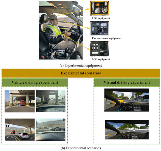
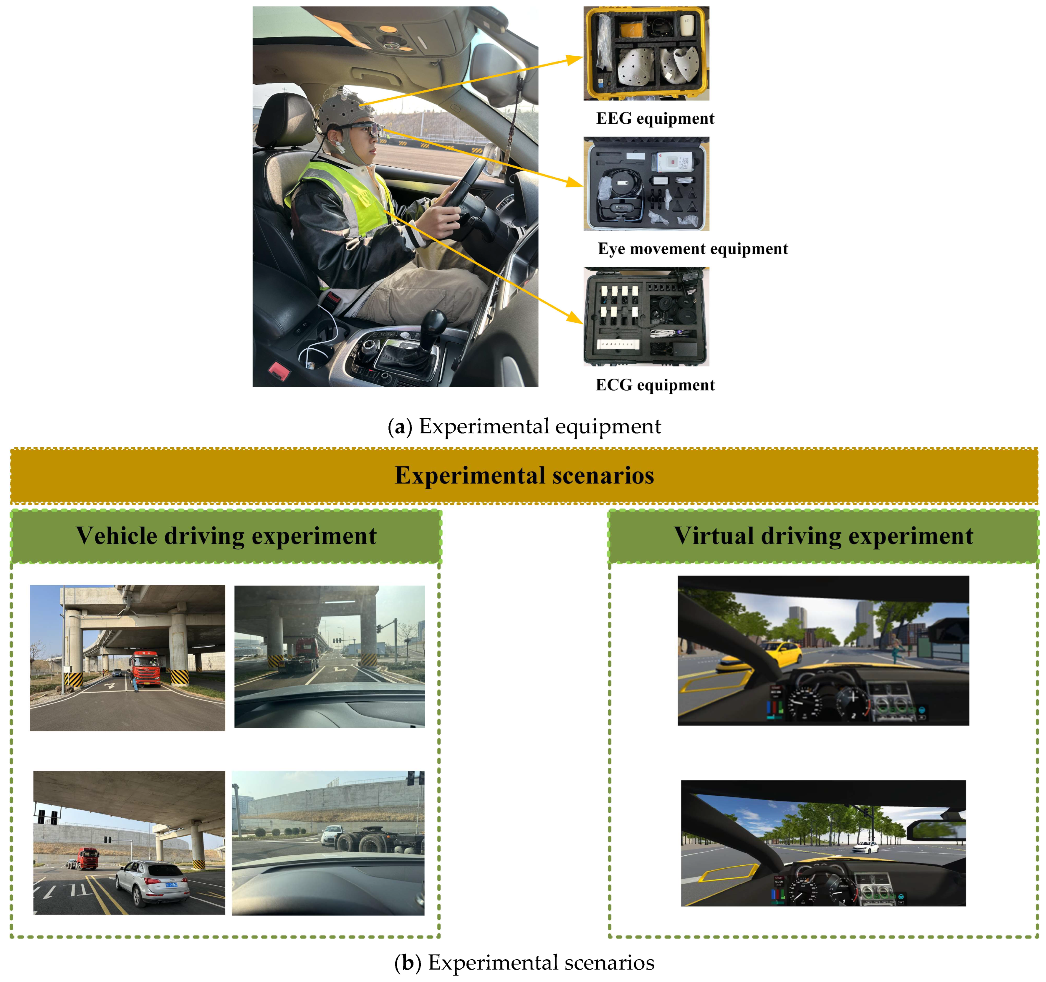
The experiment mainly includes the vehicle driving experiment and virtual driving experiment. EEG, ECG and eye movement data are collected. The vehicle driving test site is located at the National Intelligent Connected Innovation Center-Vehicle-Road Cloud Integration Test Demonstration Base in Zhaoyuan City, Shandong Province, China. The virtual driving experiment was carried out in a laboratory with standard lighting environment. The experimental scenario is designed on the basis of two typical ghost-peeking scenarios. The experimental equipment and scenarios are shown in Figure 1.

Figure 1. Experimental equipment, locations and scenarios.

2.3. Experimental Design

The experiments are divided into vehicle and virtual driving experiments. The experimental procedures of the two groups are similar. For safety reasons, the assistant driver at the passenger seat can brake the vehicle at any time in emergency. The participants are unaware of the study details beforehand and simply had to complete the driving tasks safely and normally within the designated experimental settings. The experimental procedure is as follows:

(1)

Before the experiment begins, the laboratory support staff verify that all experimental equipment is operational. The assistant staff helped the participants to wear all kinds of experimental equipment (including eye tracker, electroencephalograph, electrocardiograph, skin conductance and other human factors equipment). The video recording equipment is arranged inside and outside the vehicle. The video recording function of the eye tracker can record the first-person information of the driver. The external video recording system uses a drone to capture footage from a bird’s-eye view above the vehicle. After confirming everything is correct, it prepares to start the experiment.

(2)

Participants enter the experimental vehicle or the virtual driving platform. The assistant of experiment turns on each device. The participants are required to complete driving tasks in two constructed experimental scenarios according to the predetermined driving routes.

(3)

The experimental assistants record the entire experimental process with pre-installed video recording equipment. EEG, ECG and eye movement data of the participants are collected during the experiment.

(4)

After each driving task is completed. The assistant and the participant are shown the video of the driving task. Inquire and record whether the participants perceive dangerous omens and dangerous situations at the time points when they appeared;

(5)

After all participants complete their driving tasks, we save all experimental data, organize the experimental equipment, and conclude the experiment.

3. Statistical Analysis of Local Change Points in EEG Data

To determine the two time points at which drivers perceive dangerous omens and dangerous situations, this study combined the playback of experimental videos, the results of driver inquiries, and the local change point statistics of EEG data (for the specific method, please refer to reference [48]). Based on this, the data collected from the experiment were categorized into three distinct perception states (i.e., NPD, PDO, and PDS).

Local analysis [49,50] is a practical and powerful tool in the field of change point detection, especially in modern data flow and real-time monitoring applications. Its core lies in “seeing the big picture from the local”, which achieves rapid early warning of process changes by continuously scanning recent data. The data collected during the experiment are then categorized into three distinct perceptual states: NPD, PDO, and PDS. Table 1 shows the details of the sliding window parameters for EEG data in the local analysis method.

Table 1. Sliding window parameters of EEG data in the local analysis method.

	Window Length	Number of Sampling Points	Frequency of Sampling	Threshold Value	Minimum Duration
α	4 s	1000	250 Hz	μ + 3σ (p < 0.1)	0.5 s
β	4 s	1000	250 Hz	μ + 3σ (p < 0.1)	0.5 s
θ	3 s	750	250 Hz	μ + 3σ (p < 0.1)	0.3 s
δ	3 s	750	250 Hz	μ + 3σ (p < 0.1)	0.3 s
γ	3 s	750	250 Hz	μ + 3σ (p < 0.1)	0.3 s

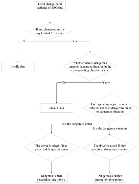
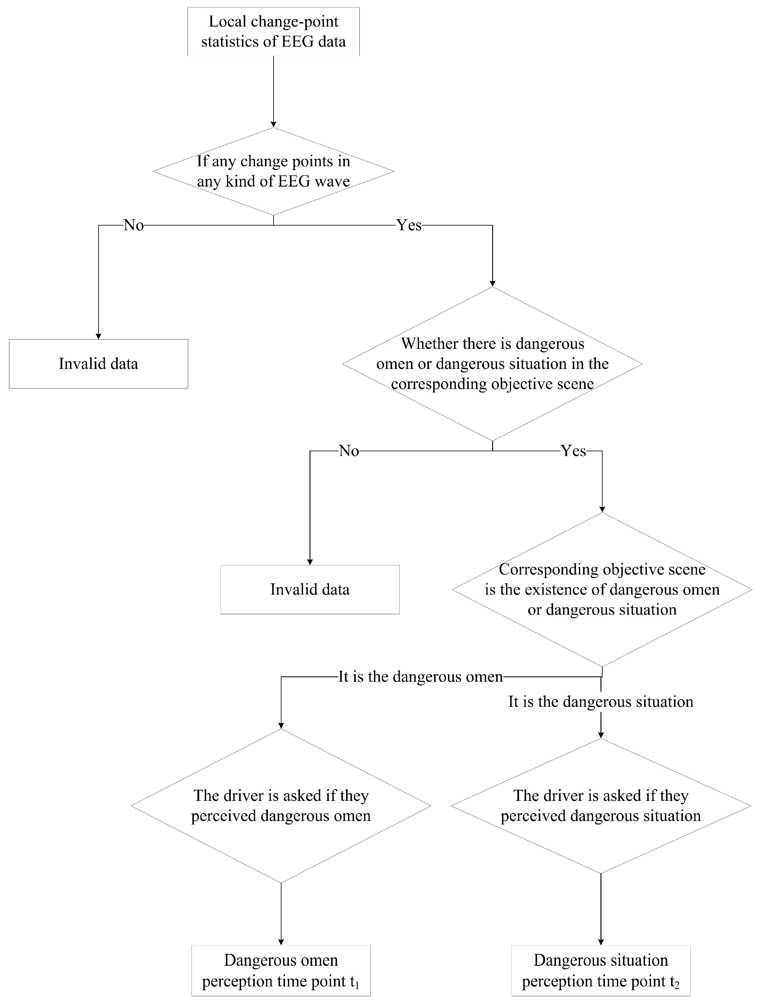
Local variable point analysis of α, β, θ, δ and γ waves are performed for each driver. In this study, a combined variable point detection strategy utilizing multiple types of brain waves is employed. The experiment video playback and the active inquiry of the driver are combined to jointly determine the time point when the driver perceives the danger signal and danger state, thus making the result more accurate. The specific procedure is as follows: apply sliding window detection to each EEG data. If no change points are detected in any of the EEG data, the driver’s data are recorded as invalid. When any kind of brainwave data detects a change point. The video playback and the active inquiry of the driver are combined, and the time point when the driver perceives the dangerous omen is recorded as $t_1$, and the time point when the dangerous situation is perceived is recorded as $t_2$.

Figure 2 shows the specific process of judging the time point of the drivers’ dangerous omen perception and dangerous situation perception.

Figure 2. Specific workflow for identifying the time points when drivers perceive dangerous omens and situation conditions. $t_1$ is the time point of dangerous omen perception, and $t_2$ is the time point of dangerous situation perception.

According to the above method, the time points of the drivers’ perception of dangerous omen and danger situation in each experimental process are obtained in this study, and some results are shown in Table 2.

Table 2. Time points of drivers’ perception of danger omens and situations (partial). “…” represents participants #9 to #65, omitted for space.

Order Number	Drivers’ Perceived Time of Dangerous Omen	Drivers’ Perceived Time of Dangerous Situation
1	139.9	169.1
2	134.9	164.4
3	129.1	161.7
4	145.1	181.6
5	163.4	198.1
6	167.3	190.1
7	146.7	175.8
8	147.6	181.1
…	…	…
66	141.4	173.6
67	153.1	187.2

For each driver, we calculated the absolute time difference $\Delta t$ between the EEG change point detection result and the driver’s self-reported time point, including both the dangerous omen perception time point and the dangerous situation perception time point. The results show that for the dangerous omen perception time point, the mean absolute deviation is 0.21 s, the standard deviation is 0.13 s, and the 95% confidence interval is [0.18 s, 0.24 s]. For the dangerous situation perception time point, the mean absolute deviation is 0.18 s, the standard deviation is 0.11 s, and the 95% confidence interval is [0.15 s, 0.21 s]. Therefore, this study selects $\Delta t\le 0.2 \mathrm{s}$ as the acceptable error range for the perception time points.

Before data analysis, the raw EEG, ECG, and eye movement data are preprocessed. EEG data are filtered using a 0.5–50 Hz bandpass filter, and independent component analysis is applied to remove ocular and myoelectric artifacts. ECG data are processed using a 0.5–40 Hz bandpass filter. The eye movement data are smoothed using median filtering to eliminate transient interference such as blinks.

4. Analysis of Physiological Characteristics of Drivers in Different Sensory States

In this study, the EEG, ECG and eye movement characteristics of the three states of NPD, PDO and PDS are statistically analyzed and compared. The characteristics of drivers in different stages of the experiment are studied to explore the law of drivers’ perceptual state transfer. So we can judge whether the driver can really perceive the dangerous omen and clearly distinguish the dangerous omen from the dangerous situation. Through experiments, the EEG, ECG, and eye movement data of 67 participants during vehicle and virtual driving tests are collected, with selected data examples are shown in Table 3. The EEG data includes alpha waves, beta waves, theta waves, delta waves, and gamma waves. The eye movement data included gaze velocity (GV), left pupil diameter (LPD), and right pupil diameter (RPD).

Table 3. Examples of experimental data (partial). “…” represents participants #9 to #65, omitted for space.

Number	α (μV2/Hz)	β (μV2/Hz)	θ (μV2/Hz)	δ (μV2/Hz)	γ (μV2/Hz)	GV (px/ms)	LPD (mm)	RPD (mm)	ECG (μV)
1	2.21 × 10−13	1.34 × 10−13	3.36 × 10−13	1.27 × 10−12	9.36 × 10−14	0.023	4.084	3.96	−12.687
2	2.32 × 10−13	1.01 × 10−13	2.90 × 10−13	2.16 × 10−13	5.15 × 10−14	0.008	4.0745	3.958	−6.156
3	1.44 × 10−13	7.60 × 10−14	2.43 × 10−13	5.96 × 10−13	4.68 × 10−14	0.018	4.021	3.941	−2.832
4	1.87 × 10−13	1.10 × 10−13	5.28 × 10−13	2.10 × 10−12	5.56 × 10−14	0.076	4.0145	3.941	19.475
5	7.57 × 10−13	2.11 × 10−13	2.43 × 10−12	1.02 × 10−11	1.03 × 10−13	0.062	4.001	3.900	−3.662
6	5.23 × 10−13	1.49 × 10−13	3.74 × 10−12	1.32 × 10−11	1.20 × 10−13	0.074	2.9825	3.878	−13.192
7	1.38 × 10−12	1.51 × 10−12	2.79 × 10−12	1.40 × 10−11	3.98 × 10−13	0.355	2.9805	3.848	17.327
8	2.27 × 10−12	2.47 × 10−13	2.72 × 10−11	8.58 × 10−11	6.44 × 10−14	0.288	4.0075	3.889	−3.053
…	…	…	…	…	…	…	…	…	…
66	1.15 × 10−12	5.61 × 10−13	7.22 × 10−12	3.87 × 10−11	1.85 × 10−13	0.321	4.0155	3.828	−18.363
67	1.30 × 10−12	2.33 × 10−13	2.43 × 10−11	8.79 × 10−11	1.20 × 10−13	0.192	4.036	3.831	25.205

The descriptive statistics of EEG data are shown in Table 4.

Table 4. Descriptive statistics of driver’s EEG, ECG, and eye movement data.

Driver Characteristics	Driver Perception State	Total N	Average Value (μV2/Hz)	Standard Deviation	95% Confidence Interval of the Mean		Minimum Value (μV2/Hz)	Maximum Value (μV2/Hz)
					Lower Limit	Upper Limit
EEG-α	NPD	67	1.139 × 10−12	2.185 × 10−12	6.061 × 10−13	1.672 × 10−12	8.180 × 10−14	1.650 × 10−11
	PDO	67	6.261 × 10−13	6.328 × 10−13	4.718 × 10−13	7.805 × 10−13	1.050 × 10−13	4.270 × 10−12
	PDS	67	5.080 × 10−12	8.696 × 10−12	2.959 × 10−12	7.201 × 10−12	9.360 × 10−14	4.800 × 10−11
EEG-β	NPD	67	3.466 × 10−13	7.237 × 10−13	1.701 × 10−13	5.232 × 10−13	7.500 × 10−14	5.000 × 10−12
	PDO	67	1.762 × 10−13	8.857 × 10−14	1.546 × 10−13	1.978 × 10−13	8.150 × 10−14	5.850 × 10−13
	PDS	67	7.471 × 10−13	2.133 × 10−12	2.268 × 10−13	1.267 × 10−12	7.140 × 10−14	1.570 × 10−11
EEG-θ	NPD	67	8.379 × 10−12	1.228 × 10−11	5.384 × 10−12	1.137 × 10−11	2.330 × 10−13	6.090 × 10−11
	PDO	67	3.876 × 10−12	8.625 × 10−12	1.772 × 10−12	5.979 × 10−12	2.910 × 10−13	5.120 × 10−11
	PDS	67	5.566 × 10−11	1.133 × 10−10	2.804 × 10−11	8.329 × 10−11	2.350 × 10−13	8.360 × 10−10
EEG-δ	NPD	67	3.465 × 10−11	5.400 × 10−11	2.148 × 10−11	4.782 × 10−11	2.160 × 10−13	3.420 × 10−10
	PDO	67	1.535 × 10−11	2.676 × 10−11	8.818 × 10−12	2.187 × 10−11	5.840 × 10−13	1.220 × 10−10
	PDS	67	2.505 × 10−10	6.927 × 10−10	8.152 × 10−11	4.194 × 10−10	9.550 × 10−13	5.450 × 10−09
EEG-γ	NPD	67	1.414 × 10−13	2.891 × 10−13	7.092 × 10−14	2.120 × 10−13	2.880 × 10−14	2.010 × 10−12
	PDO	67	7.946 × 10−14	3.098 × 10−14	7.190 × 10−14	8.701 × 10−14	3.640 × 10−14	2.100 × 10−13
	PDS	67	1.744 × 10−13	3.833 × 10−13	8.086 × 10−14	2.679 × 10−13	2.330 × 10−14	2.810 × 10−12

The descriptive statistics of ECG data are shown in Table 5.

Table 5. Descriptive statistics of driver’s ECG.

Driver Characteristics	Driver Perception State	Total N	Average Value (μV2/Hz)	Standard Deviation	95% Confidence Interval of the Mean		Minimum Value (μV2/Hz)	Maximum Value (μV2/Hz)
ECG	NPD	67	−2.407	18.351	−6.883	2.069	−40.581	37.169
	PDO	67	−16.723	42.115	−26.995	−6.450	−174.119	77.090
	PDS	67	5.125	68.135	−11.405	21.834	−219.497	186.113

The descriptive statistics of eye movement data are shown in Table 6.

Table 6. Descriptive statistics of driver’s eye movement data.

Driver Characteristics	Driver Perception State	Total N	Average Value (μV2/Hz)	Standard Deviation	95% Confidence Interval of the Mean		Minimum Value (μV2/Hz)	Maximum Value (μV2/Hz)
Eye movement-GV	NPD	67	0.230	0.364	0.141	0.319	0.008	2.530
	PDO	67	0.212	0.293	0.140	0.283	0.010	1.830
	PDS	67	1.113	1.416	0.767	1.458	0.180	6.637
Eye movement-LPD	NPD	67	4.169	0.446	4.061	4.278	2.623	4.896
	PDO	67	3.099	0.739	2.919	3.280	2.200	4.624
	PDS	67	3.280	0.844	3.075	3.486	1.915	4.579
Eye movement-RPD	NPD	67	4.148	0.237	4.090	4.206	3.575	4.577
	PDO	67	3.688	0.282	3.619	7.757	3.176	4.418
	PDS	67	3.665	0.378	3.573	3.757	2.888	4.494

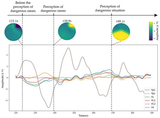
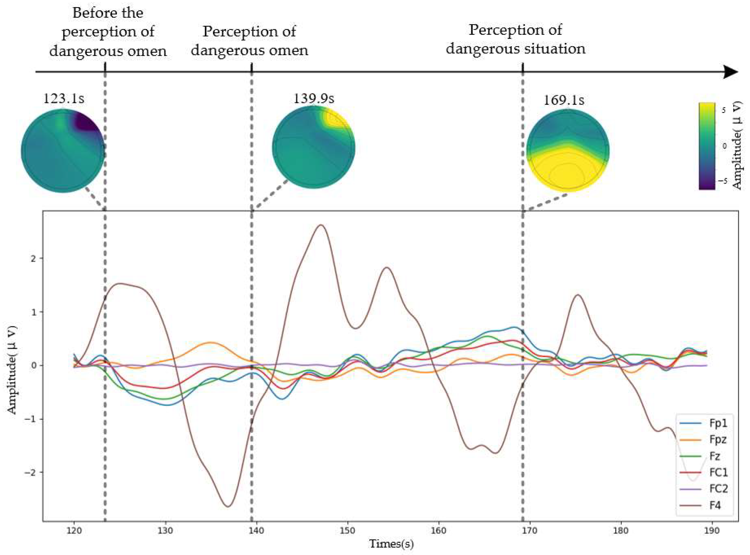
Figure 3 shows the EEG changes of the 16th driver during the vehicle driving experiment under different states (NPD, PDO and PDS). The six curves in Figure 3 represent the electrical signal variations in the driver’s brain at the following locations: frontal pole 1 (Fp1), frontal pole zero (Fpz), frontal zero (Fz), frontal central 1 and 2 (FC1 and FC2), and right frontal lobe (F4).

Figure 3. EEG data sample of the 16th driver in the experimental driving test.

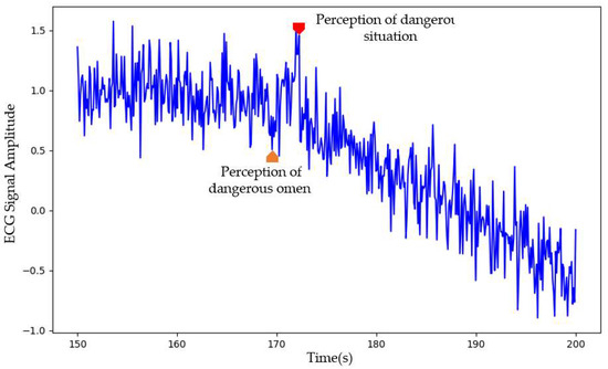
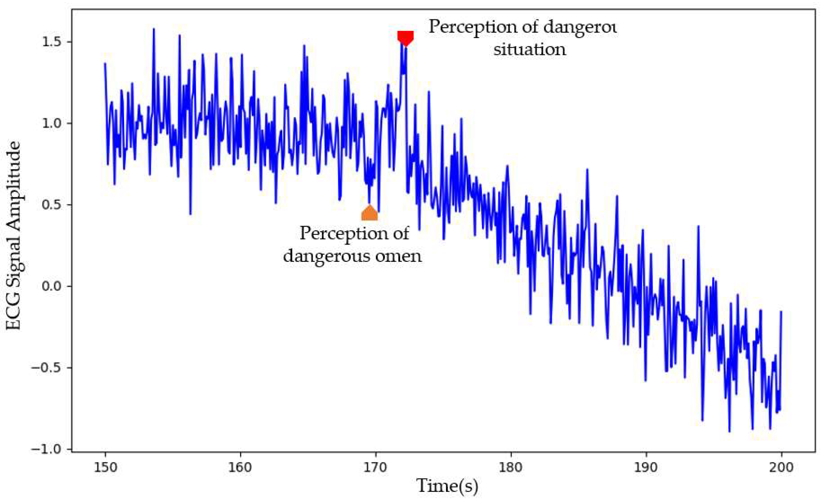
Figure 4 shows the ECG changes of the 31st driver during the vehicle driving experiment under three conditions (NPD, PDO and PDS).

Figure 4. ECG data sample of the 35th driver in the real-vehicle driving experiment.

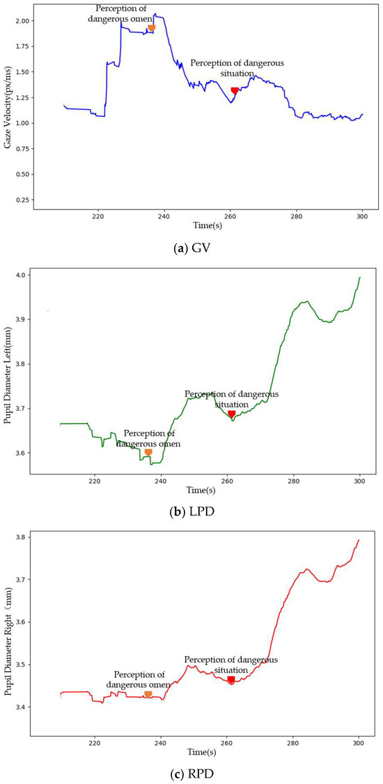
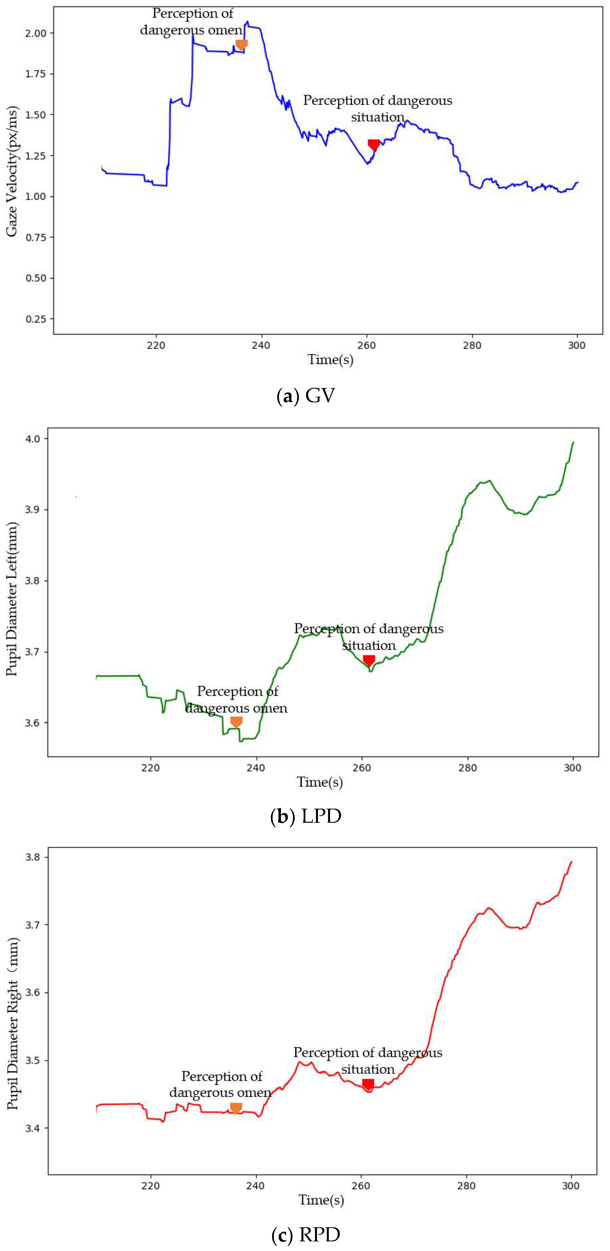
Figure 5 shows the eye movement changes of the 28th driver in the virtual driving experiment under different perceptual states (NPD, PDO and PDS).

Figure 5. Eye movement data example of the 28th driver in the virtual driving experiment.

The driver’s perception states (NPD, PDO, and PDS) are used as factor variables. EEG (α, β, θ, δ, and γ waves), ECG, and eye movement (GV, LPD, and RPD) data are used as dependent variables respectively. The K-S test is performed on the data to determine whether the collected EEG data of the driver meets the normal distribution condition. The results of the K-S test are shown in Table 7.

Table 7. K-S test results of driver’s EEG, ECG, and eye movement data.

	Kolmogorov–Smirnov (V) a
	Test Statistics	Free Degree	Conspicuousness
EEG-α	0.346	201	0.000
EEG-β	0.395	201	0.000
EEG-θ	0.374	201	0.000
EEG-δ	0.405	201	0.000
EEG-γ	0.352	201	0.000
ECG	0.147	201	0.000
Eye movement-GV	0.297	201	0.000
Eye movement-LPD	0.256	201	0.000
Eye movement-RPD	0.041	201	0.000

Pour: ^a Lilly’s significance correction.

Table 7 indicates that the significance levels of the driver’s EEG, ECG, and eye movement data are all below 0.05 (p < 0.001). The normality assumption is rejected, and the data did not conform to a normal distribution. Therefore, non-parametric tests are conducted on the EEG, ECG, and eye movement data under different perceptual states. Since the dataset comprises three samples (NPD, PDO, and PDS). The K-W test is selected for this study, with the results are shown in Table 8.

Table 8. K-W test results of EEG, ECG, and eye movement data under different driver perception states.

	Total N	Test Statistics	Free Degree	Stepwise Significance (Two-Tailed Test)
EEG-α	201	35.794 a	2	0.000
EEG-β	201	6.759 a	2	0.000
EEG-θ	201	45.995 a	2	0.034
EEG-δ	201	47.977 a	2	0.000
EEG-γ	201	7.063 a	2	0.029
ECG	201	1.660 a	2	0.436
Eye movement-GV	201	50.388 a	2	0.000
Eye movement-LPD	201	56.857 a	2	0.000
Eye movement-RPD	201	75.940 a	2	0.000

Pour: ^a The test statistics will adjust for the bound values.

In the K-W test, the null hypothesis of this study is that the driver’s perceived state differed. The distributions of alpha wave, beta wave, theta wave, delta wave, gamma wave, ECG, GV, LPD, and RPD data are the same. Table 6 shows that the significance of the data for alpha wave (p < 0.001), beta wave (p < 0.001), theta wave (p = 0.034), delta wave (p < 0.001), gamma wave (p = 0.029), GV (p < 0.001), LPD (p < 0.001), and RPD (p < 0.001) is less than 0.05 in the NPD, PDO, and PDS states, thus rejecting the null hypothesis. Therefore, the data distributions of alpha wave, beta wave, theta wave, delta wave, gamma wave, GV, LPD, and RPD differ significantly in the NPD, PDO, and PDS states.

Drivers exhibit different EEG and eye-tracking characteristics in the three perceptual states of NPD, PDO, and PDS. Since the p-value for ECG (p = 0.436) was greater than 0.05, the null hypothesis was retained, indicating that the distribution of ECG data was the same across the NPD, PDO, and PDS conditions, with no significant differences. Further multiple comparison analysis is performed to examine the significant differences in each characteristic between any two different perceptual states (i.e., between any two of NPD, PDO, and PDS). Since no significant differences were found in the distribution of the ECG data, post hoc tests were not conducted. The results are shown in Table 9.

Table 9. Paired Comparison Results.

	Sample 1-Sample 2	Test Statistics	Standard Test Statistics	Significance	Adj. Significance a
EEG-α	PDO-PDS	15.687	1.561	0.000	0.000
	PDO-NPD	−58.104	−5.782	0.000	0.000
	PDS-NPD	−42.418	−4.221	0.000	0.000
EEG-β	PDO-PDS	−22.201	−2.212	0.000	0.000
	PDO-NPD	22.978	2.289	0.000	0.000
	PDS-NPD	0.776	0.077	0.000	0.000
EEG-θ	PDO-PDS	19.560	1.946	0.013	0.041
	PDO-NPD	−66.321	−6.599	0.000	0.000
	PDS-NPD	−46.761	−4.653	0.000	0.000
EEG-δ	PDO-PDS	18.440	1.835	0.000	0.000
	PDO-NPD	−67.351	−6.702	0.000	0.000
	PDS-NPD	−48.910	−4.867	0.000	0.000
EEG-γ	PDO-PDS	−8.560	−0.856	0.003	0.010
	PDO-NPD	−26.075	−2.607	0.009	0.027
	PDS-NPD	17.515	1.751	0.008	0.024
Eye movement-GV	NPD-PDO	6.224	0.619	0.000	0.000
	NPD-PDS	−64.657	−6.434	0.000	0.000
	PDO-PDS	−58.433	−5.814	0.000	0.000
Eye movement-LPD	NPD-PDO	−10.134	−1.008	0.000	0.000
	NPD-PDS	70.104	6.976	0.000	0.000
	PDO-PDS	59.970	5.967	0.000	0.000
Eye movement-RPD	NPD-PDO	−1.007	−0.100	0.000	0.000
	NPD-PDS	76.343	7.596	0.000	0.000
	PDO-PDS	75.336	7.496	0.000	0.000

Pour: ^a Adjusted for multiple comparisons using the Bonferroni correction.

As shown in Table 9, the significance of the α-wave, β-wave, θ-wave, δ-wave, γ-wave, GV, LPD, and RPD data between any two different perceptual states of the driver is less than 0.05. Therefore, there are significant differences in the α-wave, β-wave, θ-wave, δ-wave, γ-wave, GV, LPD, and RPD data between different perceptual states of the driver. Drivers exhibit different EEG, and eye movement characteristics in each perception state.

5. Driver Perception State Transition Model Based on Hidden Markov Model

5.1. Model Construction

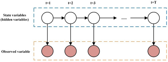
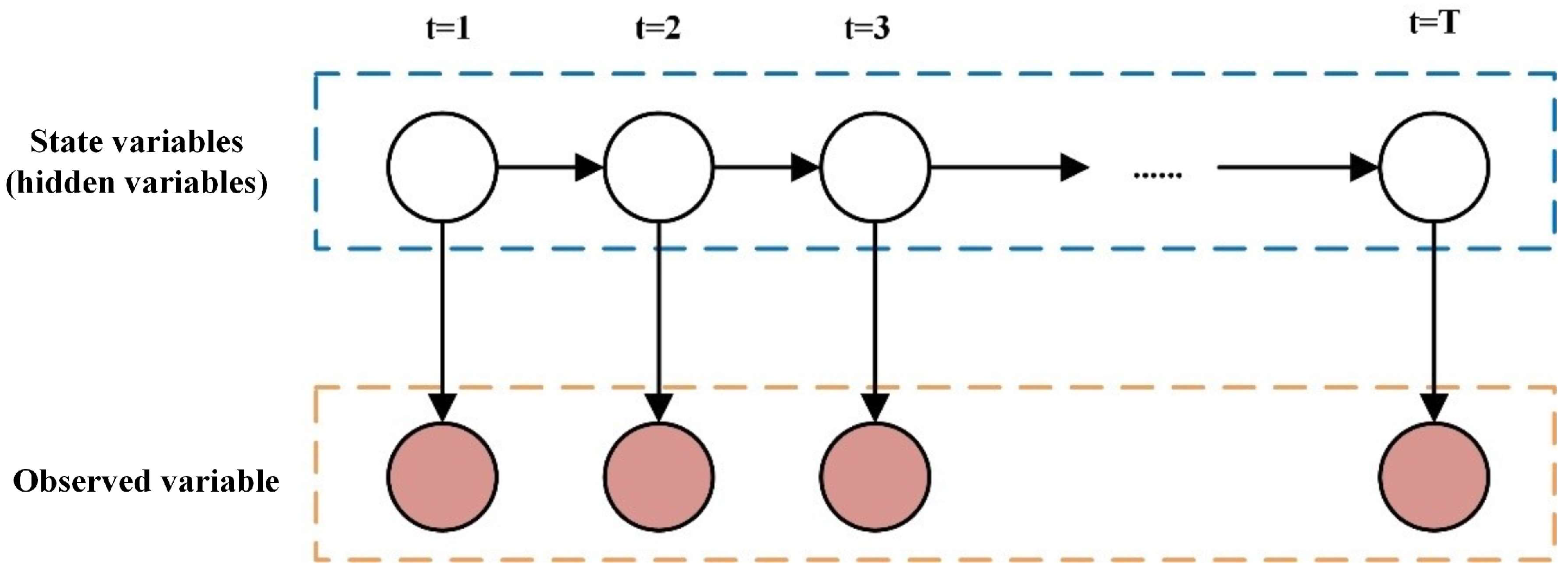
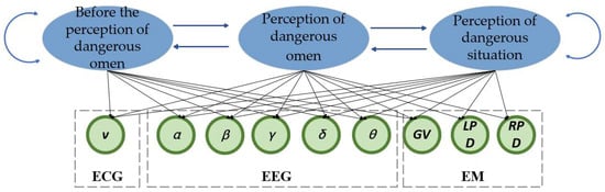
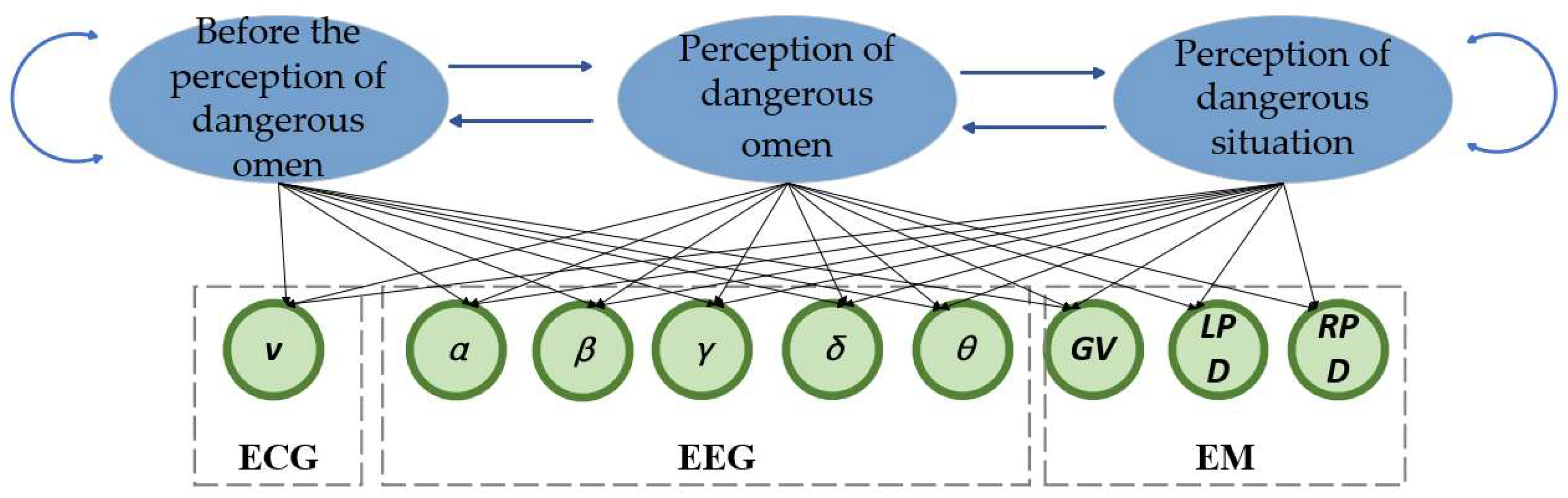
HMM (Hidden Markov Model) is a statistical model to describe a system consisting of hidden states and observable events [51]. In this study, HMM is adopted for the following reasons: (1) it offers clear interpretability, as the state transition probabilities directly reflect the evolution patterns of perceptual states; (2) it is suitable for small sample scenarios, with fewer parameters compared to deep learning models such as LSTM or GRU; (3) its Markov assumption aligns well with the characteristics of driver perception evolution, where the next state primarily depends on the current state. It is assumed that the states of the system cannot be directly observed and they are inferred through the associated observation data. HMM consists of three main components: hidden states, observation probabilities, and transition probabilities. In HMM, a transition pattern exists between system states. Each state generates an observation value based on a certain probability distribution. HMM is widely used in tasks such as time series analysis, speech recognition, and natural language processing. It can model the hidden structure of dynamic systems and inferring potential state changes. The structure is shown in Figure 6.

Figure 6. Hidden Markov Algorithm Structure.

HMM has a natural advantage in time series modeling. They can effectively capture the changing processes of system states and are particularly suitable for describing the relationship between latent states (such as NPD, PDO, and PDS) and observed data (such as EEG, ECG, and eye-tracking data). In this study, the driver’s perception state is constantly changing, and these changes could not be directly observed. HMM can be used to infer the potential driver’s perception state from the observed data. By setting state transition probabilities, HMM can model these state changes very naturally. This is suitable for studying the drivers’ perception of state transition patterns in this study.

In this study, HMM consists of three hidden states, corresponding to NPD, PDO, and PDS, respectively. The observation sequence is composed of EEG, ECG, and eye movement features, as shown in Figure 7. Each feature is normalized using the Z-score method before being input into the model. The initial state probability vector π is set to a uniform distribution. The state transition probability matrix A and the observation probability matrix B are estimated using the Baum-Welch algorithm, with the convergence criterion set to a change in the log-likelihood function of less than 10⁻⁴. The model is validated using 5-fold cross-validation.

Figure 7. Schematic diagram of Hidden Markov Model. In the observed data, “v” denotes the ECG signal value, and “EM” denotes eye movement.

The basic formula for HMM is as follows:

$$P(X,Y)=P(Y_1){\displaystyle \prod _{t=2}^{T}P(Y_t\left|Y_{t-1}\right.)P(X_t\left|Y_t\right.)}$$

(1)

$P(Y_1)$ represents the probability distribution of the initial state. $P(Y_t\left|Y_{t-1}\right.)$ represents the state transition probability, indicating the probability of transitioning from time t − 1 to time t. $P(X_t\left|Y_t\right.)$ is the emission probability, representing the probability of observing data X_t given a hidden state Y_t. X represents the sequence of observed data. Y represents the sequence of hidden states. HMM is trained by learning the state transition matrix and emission matrix of the data. The model can predict the state at each time and calculate the probability of each state. In this study, HMM is employed to model three states (NPD, PDO, and PDS). Consider a Hidden Markov Model with three states:

$$S=\{S_0,S_1,S_2\}$$

(2)

Here, $S_0$ denotes the NPD state, $S_1$ the PDO state, and $S_2$ the PDS state. Through training with the observation sequence $O=\{o_1,o_2,\dots ,o_T\}$, the HMM learns the state transition probability A and the observation probability B, as follows:

The state transition matrix A represents the probability of transitioning from one state to another:

$$A=\left(\begin{array}{l}{a}_{00}{a}_{01}{a}_{02}\\ a_{10}{a}_{11}{a}_{12}\\ a_{20}{a}_{21}{a}_{22}\end{array}\right)$$

(3)

$a_{00}$ denotes the probability that the driver remains in the non-perception state; $a_{01}$ denotes the probability that the driver transitions from the non-perception state to the dangerous omen perception state; $a_{02}$ denotes the probability that the driver transitions directly from the non-perception state to the dangerous situation perception state; $a_{10}$ denotes the probability that the driver returns from the dangerous omen perception state to the non-perception state; $a_{11}$ denotes the probability that the driver remains in the dangerous omen perception state; $a_{12}$ denotes the probability that the driver transitions from the dangerous omen perception state to the dangerous situation perception state; $a_{20}$ denotes the probability that the driver returns from the dangerous situation perception state to the non-perception state; $a_{21}$ denotes the probability that the driver transitions from the dangerous situation perception state to the dangerous omen perception state; $a_{22}$ denotes the probability that the driver remains in the dangerous situation perception state.

The observation probability matrix $B$ represents the probability of observing a specific value in each state:

$$B=\left(\begin{array}{l}{b}_0(o_1)b_0(o_2)\dots b_0(o_T)\\ b_1(o_1)b_1(o_2)\dots b_1(o_T)\\ b_2(o_1)b_2(o_2)\dots b_2(o_T)\end{array}\right)$$

(4)

The probability of the system in different states at each time is obtained by training the model and predicting the most probable state sequence corresponding to the given observation sequence. To better verify the output results of the model, this study uses a linear regression (LR) model [52] to model the changing trends of different driver characteristics (EEG, ECG, and eye movement) based on the state sequence predicted by the HMM. The regression coefficient is estimated by minimizing the error between the predicted value and the true value. This objective can be achieved by the least squares method, as shown in Formula (5).

$$\stackrel{\wedge }{\sigma }=\arg \underset{\sigma }{\min }{\displaystyle \sum _{t=1}^T(Y_t-{({\sigma }_0+({\displaystyle \sum _{i=1}^n{\sigma }_i{X}_{i,t}+}{\sigma }_0))}^2}$$

(5)

where $\widehat{\sigma }$ represents the regression coefficient estimate obtained by minimizing the error. The least squares method can be used to find the $\sigma$ series that minimizes the difference between the predicted value and the true value. $Y_t$ represents the predicted value at time $t$, $X_i$ represents the $i$-th parameter at time $t$, and ${\sigma }_i$ is the regression coefficient. The regression equation can be used to evaluate the relationship between each feature and the driver’s perception state. The form of the regression model is shown in (6).

$$Y_t={\displaystyle \sum _{i=1}^n{\sigma }_i{X}_{i,t}+}{\sigma }_0$$

(6)

where ${\sigma }_i$ (i = 0, 1, …, n) are the regression coefficients, ${\sigma }_0$ is the intercept term, and $X_{i,t}$ denotes the i-th feature observed at time t.

5.2. Model Calibration

The experimental data of 67 drivers are collected in this study. Except for two invalid datasets, the data of 55 drivers are used to calibrate the model. The data of the remaining 10 drivers are used to verify the model. The results of non-parametric test on the EEG, ECG and eye movement data show that the α, β, θ, δ and γ waves in EEG, GV, LPD and RPD in eye movement are all significantly related to the drivers’ perception state, and the ECG is not correlated. Therefore, the feature data with significant correlations mentioned above are used as input for the HMM to calibrate the model.

In order to better calibrate the HMM, the Baum-Welch estimation algorithm is adopted in this study for parameter selection and optimization. The specific method can be found in reference [53], and will not be repeated here, and the method of k-fold (k = 5) cross-validation was adopted. Finally, the obtained driver perception state transition probability matrix is shown in Equation (7):

$$P_{ij}=\left[\begin{array}{ccc}{p}_{00}& p_{01}& p_{02}\\ p_{10}& p_{11}& p_{12}\\ p_{20}& p_{21}& p_{22}\end{array}\right]$$

(7)

Due to space limitations, this section only uses the experimental data of the 12th group of drivers in the vehicle driving experiment as an example to list the transition probability matrix of the driver’s perception state during the experiment, as shown in Formula (8).

$$\begin{array}{ccc}{P}_{00}=\left[\begin{array}{ccc}0.9971& 0.0029& 0.0000\\ 0.0000& 0.0000& 1.0000\\ 0.0132& 0.0000& 0.9868\end{array}\right]& P_{01}=\left[\begin{array}{ccc}0.0001& 0.9967& 0.0032\\ 0.8961& 0.0004& 0.1034\\ 0.0050& 0.0097& 0.9853\end{array}\right]& P_{02}=\left[\begin{array}{ccc}0.7789& 0.0790& 0.1421\\ 0.0532& 0.9468& 0.0000\\ 0.1077& 0.0000& 0.8923\end{array}\right]\\ P_{10}=\left[\begin{array}{ccc}0.0001& 0.9967& 0.0032\\ 0.8961& 0.0004& 0.1034\\ 0.0050& 0.0097& 0.9853\end{array}\right]& P_{11}=\left[\begin{array}{ccc}0.9952& 0.0048& 0.0000\\ 0.0000& 0.9954& 0.0046\\ 0.0139& 0.0000& 0.9861\end{array}\right]& P_{12}=\left[\begin{array}{ccc}0.9493& 0.0507& 0.0000\\ 0.1490& 0.5729& 0.2781\\ 0.0000& 0.0518& 0.9482\end{array}\right]\\ P_{20}=\left[\begin{array}{ccc}0.9321& 0.0679& 0.0000\\ 0.1329& 0.8610& 0.0061\\ 0.1244& 0.2105& 0.6652\end{array}\right]& P_{21}=\left[\begin{array}{ccc}0.9321& 0.0679& 0.0000\\ 0.1329& 0.8610& 0.0061\\ 0.1244& 0.2105& 0.6652\end{array}\right]& P_{22}=\left[\begin{array}{ccc}0.9188& 0.0812& 0.0000\\ 0.0526& 0.9474& 0.0000\\ 0.0000& 0.0026& 0.9974\end{array}\right]\end{array}$$

(8)

To facilitate further validation of the model, the constructed regression model is calibrated in this study, as shown in Equation (6). The regression coefficients and intercept values of the obtained model are shown in Table 10.

Table 10. Model regression coefficients and intercept values.

Observation Sequence		Regression Coefficient	Value	Observation Sequence		Regression Coefficient	Value
EEG-α	$X_1$	${\sigma }_1$	−0.392	Eye movement-GV	$X_6$	${\sigma }_6$	0.061
EEG-β	$X_2$	${\sigma }_2$	0.567	Eye movement-LPD	$X_7$	${\sigma }_7$	−0.110
EEG-θ	$X_3$	${\sigma }_3$	−0.253	Eye movement-RPD	$X_8$	${\sigma }_8$	0.600
EEG-δ	$X_4$	${\sigma }_4$	0.403	Intercept		${\sigma }_0$	1.231
EEG-γ	$X_5$	${\sigma }_5$	−0.160

5.3. Model Validation

To verify the effectiveness of the model, five evaluation metrics were introduced into this study: mean squared error (MSE), coefficient of determination (R²), root mean square error (RMSE), mean absolute error (MAE), and mean absolute percentage error (MAPE) [54].

Specifically, MSE is used to evaluate the prediction error of a model. RMSE is the square root of MSE. R² measures how well the model fits the data. MAE is the average of the absolute values of the differences between the predicted and actual values. MAPE is a measure of the error between the predicted and actual values, and its specific calculation formula is as follows:

$$MSE={\displaystyle \frac{1}{n}}{\displaystyle \sum _{i=1}^n{(y_i-{\widehat{y}}_i)}^2}$$

(9)

$$RMSE=\sqrt{{\displaystyle \frac{1}{n}}{\displaystyle \sum _{i=1}^n{(y_i-{\widehat{y}}_i)}^2}}$$

(10)

$$R^2=1-{\displaystyle \frac{{\displaystyle {\sum }_{i=1}^n{(y_i-{\widehat{y}}_i)}^2}}{{\displaystyle {\sum }_{i=1}^n{(y_i-{\overline{y}}_i)}^2}}}$$

(11)

$$MAE={\displaystyle \frac{1}{n}}{\displaystyle \sum _{i=1}^n\left|y_i-{\widehat{y}}_i\right|}$$

(12)

$$MAPE={\displaystyle \frac{1}{n}}{\displaystyle \sum _{i=1}^n\left|{\widehat{y}}_i-y_i\right|}$$

(13)

Here, $y_i$ is the true value of the driver’s perception state, ${\stackrel{\wedge }{y}}_i$ is the predicted value of the driver’s perception state, n is the number of samples, and ${\stackrel{-}{y}}_i$ is the mean of the true values of the driver’s perception state.

In addition, linear regression, support vector machine (SVR) [55], decision tree (DT) [56], Gradient Boosting (GB) [57], and XGBoost [58] models are introduced. These models cover a range of algorithm types, from linear to nonlinear, and from single models to ensemble methods, providing a comprehensive and representative performance benchmark for the proposed HMM-LR framework.

To avoid data leakage, this study first stratified the data of 67 drivers according to their perception state labels (NPD, PDO, PDS), and randomly selected 10 drivers (approximately 15%) as an independent test set. This test set was completely isolated throughout the entire model training and hyperparameter optimization process, and was used only for final performance evaluation. The data from the remaining 55 drivers were used for model training and cross-validation. During the model training phase, 5-fold cross-validation was employed to optimize the HMM parameters and linear regression coefficients. The specific steps were as follows: the data from 55 drivers were randomly divided into five mutually exclusive subsets, with the proportion of the three perception states (NPD, PDO, PDS) in each subset kept consistent with the original data. Each time, four subsets were selected as the training set and the remaining subset as the validation set, and this process was repeated five times so that each subset was used as the validation set once. After each validation, evaluation metrics such as MSE, R², MAE, RMSE, and MAPE were calculated, and the average of the five validation results was taken as the cross-validation performance. Throughout the cross-validation process, all data from the same driver were always kept within the same subset, ensuring that no data leakage occurred between the training and validation sets. Based on the cross-validation, to further evaluate the stability of the model, the above 5-fold cross-validation was repeated 10 times (with random data partitioning each time), and the 95% confidence intervals for each evaluation metric were calculated. Finally, the previously reserved independent test set of 10 drivers was used to perform the final test on the model, yielding the generalization performance of the model. The evaluation metrics and confidence intervals for each model are shown in Table 11.

Table 11. Model Evaluation Indicators.

	MSE	R2	MAE	RMSE	MAPE
HMM-LR	0.002 ± 0.0005	0.997 ± 0.001	0.004 ± 0.001	0.043 ± 0.005	0.568 ± 0.12 × 1014
LR	0.275 ± 0.032	0.580 ± 0.045	0.431 ± 0.038	0.525 ± 0.041	5.482 ± 0.56 × 1014
SVR	0.095 ± 0.011	0.855 ± 0.021	0.160 ± 0.012	0.308 ± 0.019	2.030 ± 0.24 × 1014
DT	0.005 ± 0.0001	0.992 ± 0.002	0.003 ± 0.001	0.073 ± 0.008	0.216 ± 0.03 × 1014
GB	0.007 ± 0.002	0.989 ± 0.003	0.032 ± 0.005	0.084 ± 0.009	0.692 ± 0.08 × 1014
XGBoost	0.011 ± 0.003	0.984 ± 0.004	0.011 ± 0.002	0.103 ± 0.012	0.354 ± 0.05 × 1014

Note: Bold values represent the best performance in each category.

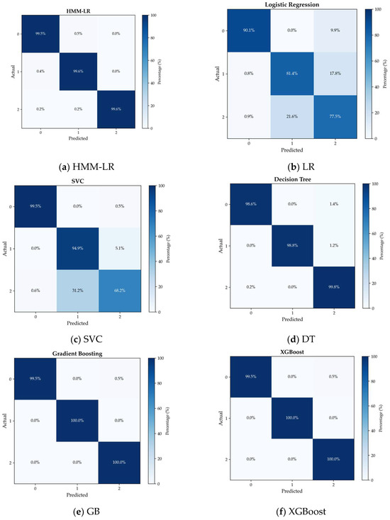
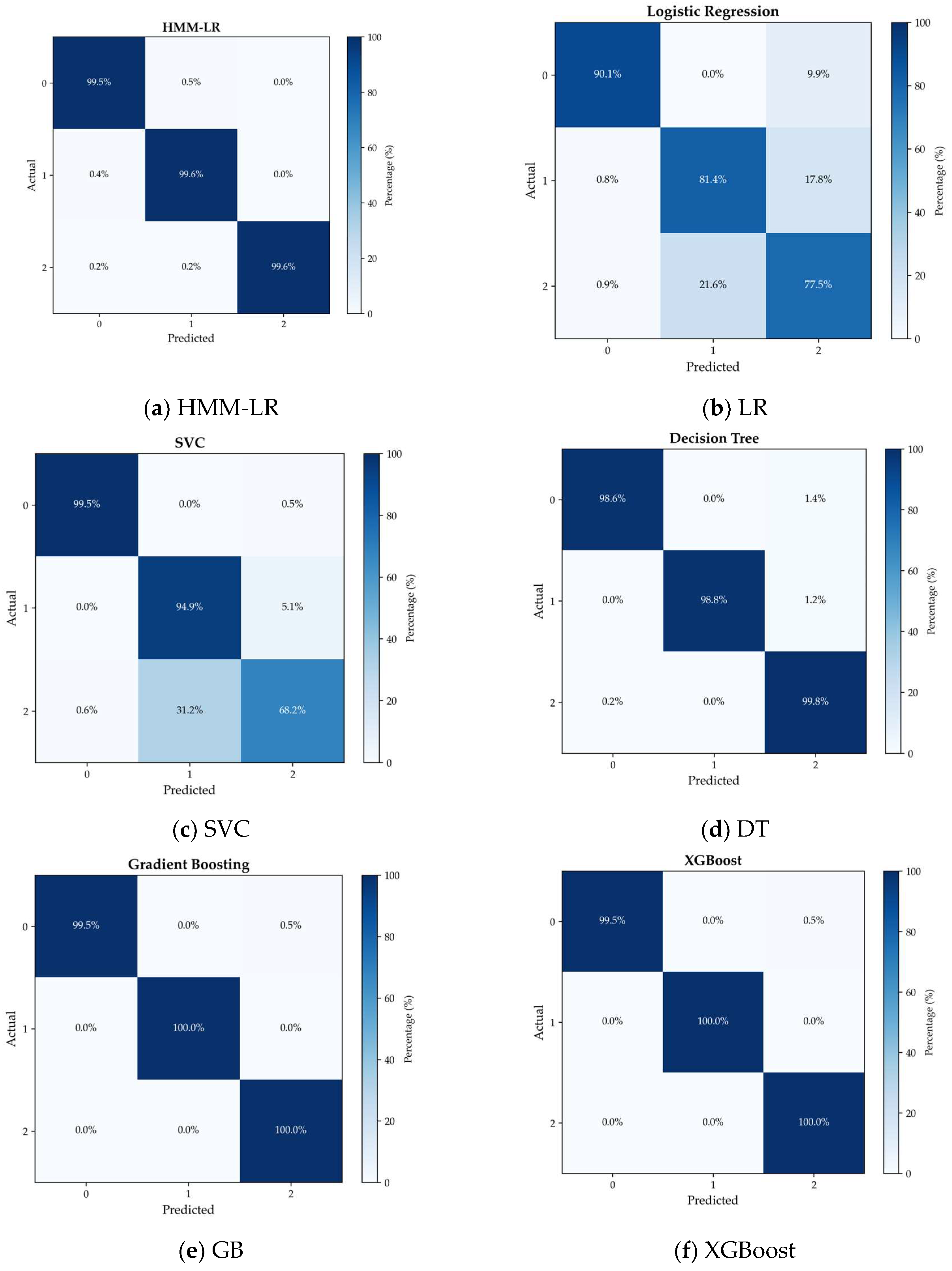
As shown in Table 9, the constructed HMM-LR model exhibits good performance. MSE and RMSE are the lowest among all models. R² is the highest among all models. MAE is only slightly higher than the decision tree model, and MAPE is only slightly higher than the decision tree model and XGBoost model. To further compare and evaluate the predictive performance of the constructed HMM-LR model. The target variable is discretized. The continuous output values are divided into several discrete categories. The regression problem is transformed into a classification problem. This allows for the evaluation of the model’s predictive accuracy. The target variable (i.e., the predicted score of the drivers’ perceived state) is assumed to be mappable to three categories: NPD (State 0), PDO (State 1), and PDS (State 2). In this study, the continuous target variable is transformed into one of these three categories. Specifically, the interval partitioning method is used in this study. The range of values for the target variable is divided into several intervals. Each interval corresponds to one of the categories: state 0, state 1, and state 2. Assuming the range of values for the target variable $y$ is $[a,b]$, each interval is partitioned according to the following rules:

$$y_{class}=\left\{\begin{array}{l}0,\mathit{if}y\in [a,m)\\ 1,\mathit{if}y\in [m,n)\\ 2,\mathit{if}y\in [n,b]\end{array}\right.$$

(14)

Here, m and n are the boundary values that divide each interval. This determines the mapping of continuous values to any one of the three class intervals, which can be obtained from the prediction model. In this way, the continuous regression output is transformed into a discrete classification task. Furthermore, the classification performance of each model is compared in this study. The resulting confusion matrix is shown in Figure 8. As shown in this figure, the constructed HMM-LR has excellent classification performance.

Figure 8. Confusion matrix.

6. Dangerous Omen Scenario Extraction Based on Driver’s Subjective Cognition

Based on the constructed driver perception state prediction model, the NPD, PDO, and PDS stages of a driver in the long-time domain before an accident can be obtained. Therefore, for any accident scenarios, drivers’ EEG, and eye-tracking data are collected and then drivers’ current perception state can be predicted. The time period when the driver perceives the dangerous omen is obtained. Then the first-person objective scenario corresponding to the subjective cognition of the driver when there is a danger is extracted. Taking two types of ghost-peeking scenarios involved in this study as examples. Based on the drivers’ perception stages in these two types of scenarios, the evolutionary patterns of “ghost-peeking” accidents in these two types of scenarios are analyzed, and the ominous scenarios are extracted. In general, dangerous omen scenarios have two objective characteristics. First, there are areas in the scenario where the driver cannot obtain information. That is, due to factors such as obstructed vision, the driver cannot obtain information about this area in a timely manner. It is difficult to determine whether there are factors affecting traffic safety in this area. In this case, the driver will perceive a dangerous omen that may lead to danger. Second, there is an area where the driver can obtain information, but the driver determines that the behavior of other road users in this area may threaten the safety of their own vehicle. In this case, the driver will perceive a hazardous sign.

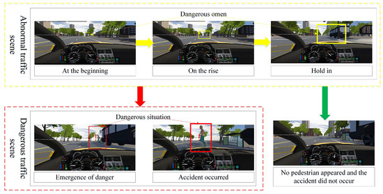
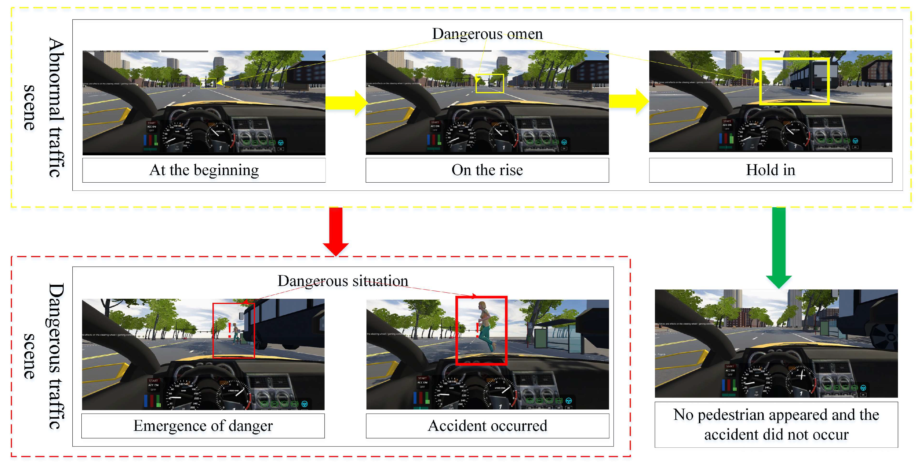
For the two types of ghost-peeking scenarios in this study, Figure 9 and Figure 10 respectively illustrate the evolution patterns of dangerous omens in these scenarios. As shown in Figure 9, when the driver’s right-side field of view is significantly obstructed by another vehicle or object, they cannot fully observe pedestrians or vehicles behind the right front. The driving scenario contains abnormal omens that may lead to danger (as shown in the yellow solid line area in Figure 9, which represents the hazard scenario requiring extraction of the driver’s first-person perspective). As the driver continues to drive, the right side remains obstructed by a vehicle, and the area of obscured vision gradually expands. The dangerous omens become increasingly prominent and persistent. If a pedestrian (or vehicle) suddenly emerges from the right front, the dangerous omens will eventually escalate into a dangerous situation (as shown by the red solid line in Figure 9), ultimately leading to an accident. If no pedestrian (or vehicle, etc.) emerges, the drivers’ view will no longer be obstructed by vehicles (or other obstructions) after passing through the area, and the dangerous omen will diminish and disappear accordingly.

Figure 9. Evolution law diagram of dangerous omens in the first type of experimental scenario. The yellow dashed box represents the dangerous omen area, and the red dashed box represents the dangerous situation area.

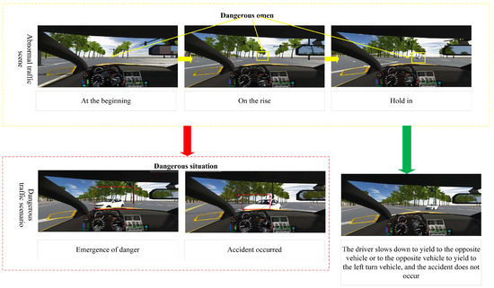
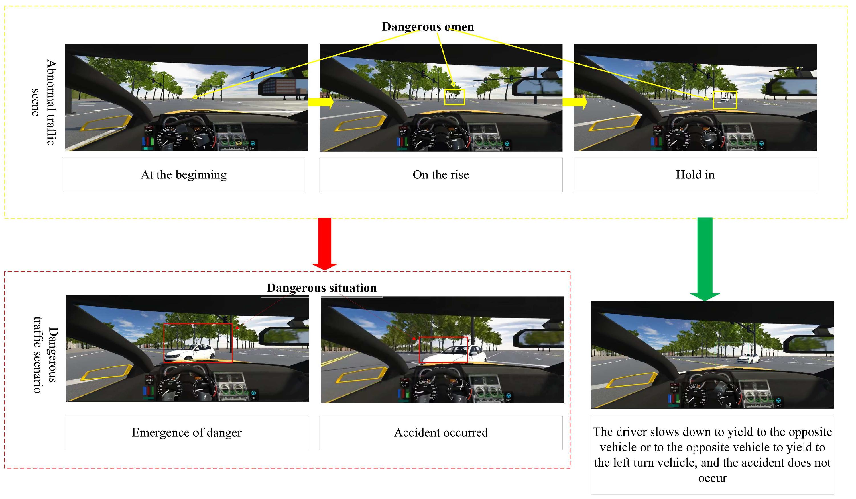
Figure 10. Evolution law diagram of dangerous omens in the second type of experimental scenario. The yellow dashed box represents the dangerous omen area, and the red dashed box represents the dangerous situation area.

As shown in Figure 10, when a driver approaches an intersection and prepares to turn left, there is a vehicle in the opposite straight lane preparing to proceed through the intersection. This vehicle is still some distance from the intersection. According to traffic rules, vehicles turning left at intersections must yield to vehicles going straight. However, because vehicles going straight in the opposite lane are far from the intersection. Drivers cannot fully judge whether the other vehicle will accelerate to cross the intersection, drive at a normal speed, or yield to the left-turning vehicle. At this time, there are dangerous signs in this area that may lead to collision accidents (As shown in the yellow solid line area in Figure 10, this represents the hazard scenario requiring extraction of the driver’s first-person perspective). As the driver drives the vehicle into the intersection and the oncoming vehicle approaches, the dangerous omen gradually increases and persists. If the oncoming vehicle accelerates to pass the intersection without yielding. There is a high probability of collision, which may escalate from the dangerous omen to the dangerous situation (as shown by the red solid line in Figure 10) and result in an accident. If the vehicle making a left turn gives way to the oncoming vehicle, or the driver slows down and yields to the oncoming vehicle. Then the dangerous omen will gradually fade and disappear after the opposite vehicle passes the intersection or the driver drives the vehicle through the intersection.

In general, according to the method proposed in this study. Any driver who can sense the danger can do it. The EEG, ECG and eye movement data can be clearly divided into three states: no perception of dangerous omens and dangerous situations, perception of dangerous omens and perception of dangerous situations. Then, the objective scenario of the first perspective corresponding to the time period of the dangerous omen perception is extracted. The extracted scenarios can be used as data samples for end-to-end large-scale learning of autonomous vehicles. It can enhance the ability of the vehicle to recognize the danger and further improve its brain-like intelligence and active safety. For example, some researchers have begun to explore the integration of traffic flow prediction with autonomous driving decision-making. The Cell-Trans method proposed by Li et al. [59] achieves high-precision trajectory prediction in signalized intersection scenarios. The dangerous omen scenarios extracted in this paper can subsequently serve as experimental scenarios for such prediction models to forecast vehicle trajectories under dangerous omen conditions.

7. Conclusions

The collection of a large number of first-person dangerous omen scenarios is of great significance for the training and improvement of end-to-end autonomous driving models. In this study, the transition patterns of drivers’ perceptual states during extended periods before accidents are thoroughly investigated. The first-person driving scenario with dangerous situation is extracted. The goal is to provide sufficient scenario data for large-scale model learning in end-to-end autonomous vehicles and enhance their capability to identify potential hazards. Based on the method proposed in this study, it is possible to determine the time periods when drivers perceive dangerous omens during driving by collecting their EEG, ECG, and eye movement data. The corresponding objective scenarios are extracted and collected. Then, this scenario is applied to end-to-end autonomous driving large model training. This study reveals the cognitive mechanisms underlying drivers’ perception of dangerous omens and promotes the development of end-to-end autonomous driving, thereby enhancing vehicle safety. In future research, we will focus on the following aspects for further investigation. First, we will extend the experimental scenarios to more complex traffic environments, such as intersections, construction zones, congested road sections, and adverse weather conditions (e.g., rain and fog), to validate the robustness and generalizability of the proposed method under different conditions. Second, we will introduce the Hidden Semi-Markov Model (HSMM) to explicitly model the duration of perceptual states, thereby further improving the accuracy of state recognition. In addition, we will explore differences in dangerous omen perception ability among driver groups of different ages, driving experience, and genders, and analyze the influence of individual heterogeneity on perceptual state transition patterns. Finally, we will integrate the dangerous omen scenarios extracted in this study with end-to-end autonomous driving models, which can evaluate their practical effectiveness in enhancing the ability of autonomous driving systems to identify potential risks.

References

- Beanland, V.; Goode, N.; Salmon, P.M.; Lenne, G. Is there a case for driver training? A review of the efficacy of pre-and post-licence driver training. Safety Sci. 2013, 51, 127–137. [Google Scholar] [CrossRef] [Scilit]
- Damm, L.; Nachtergaële, C.; Meskali, M.; Berthelon, C. The evaluation of traditional and early driver training with simulated accident scenarios. Hum. Factors 2011, 53, 323–337. [Google Scholar] [CrossRef] [Scilit] [PubMed]
- Bruce, C.; Unsworth, C.A.; Tay, R.; Dillon, P. Development and validation of the Occupational Therapy Risk Propensity Test (OT-RiPT) for drivers with disability. Scand. J. Occup. Ther. 2015, 22, 147–152. [Google Scholar] [CrossRef] [Scilit] [PubMed]
- Wu, B.; Sun, L.; Gu, N. Development and validity of a hazard prediction test for Chinese drivers. PLoS ONE 2021, 16, e0245843. [Google Scholar] [CrossRef] [Scilit] [PubMed]
- Glen, F.C.; Smith, N.D.; Crabb, D.P. Impact of superior and inferior visual field loss on hazard detection in a computer-based driving test. Br. J. Ophthalmol. 2015, 99, 613–617. [Google Scholar] [CrossRef] [Scilit]
- Malone, S.; Brünken, R. Studying gaze behavior to compare three different hazard perception tasks. Hum. Factors 2020, 62, 1286–1303. [Google Scholar] [CrossRef] [Scilit]
- Sepulveda, J.A.; Wood, J.M.; Lacherez, P.; Anderson, A.J.; McKendrick, A.M. The relationship between central and mid-peripheral motion perception and the hazard perception test in younger and older adults. Ophthalmic Physiol. Opt. 2023, 43, 1211–1222. [Google Scholar] [CrossRef] [Scilit]
- Meir, A.; Oron-Gilad, T.; Parmet, Y. Are child-pedestrians able to identify hazardous traffic situations? Measuring their abilities in a virtual reality environment. Safety Sci. 2015, 80, 33–40. [Google Scholar] [CrossRef] [Scilit]
- McInerney, K.; Suhr, J. Neuropsychological correlates of hazard perception in older adults. J. Int. Neuropsychol. Soc. 2016, 22, 332–340. [Google Scholar] [CrossRef] [Scilit]
- Sun, L.; Wang, S.; Chen, J. Development of a hazard prediction test for Chinese cyclists and its association with crash involvement. Heliyon 2023, 9, e14407. [Google Scholar] [CrossRef] [Scilit]
- Zhao, W.; Xu, L.; Bai, J.; Ji, M.; Runge, T. Sensor-based risk perception ability network design for drivers in snow and ice environmental freeway: A deep learning and rough sets approach. Soft Comput. 2018, 22, 1457–1466. [Google Scholar] [CrossRef] [Scilit]
- Lee, S.S.-Y.; Black, A.A.; Lacherez, P.; Wood, J.M. Eye movements and road hazard detection: Effects of blur and distractors. Optom. Vis. Sci. 2016, 93, 1137–1146. [Google Scholar] [CrossRef] [Scilit] [PubMed]
- Hong, I.; Kurihara, T.; Iwasaki, M. Older drivers’ perceptions, responses, and driving behaviours during complex traffic conditions at a signalized intersection. Proc. Inst. Mech. Eng. Part. D J. Automob. Eng. 2008, 222, 2063–2076. [Google Scholar] [CrossRef] [Scilit]
- Feng, J.; Choi, H.; Craik, F.I.; Levine, B.; Moreno, S.; Naglie, G.; Zhu, M. Adaptive response criteria in road hazard detection among older drivers. Traffic Inj. Prev. 2018, 19, 141–146. [Google Scholar] [CrossRef] [Scilit]
- Yamani, Y.; Horrey, W.J.; Liang, Y.; Fisher, D.L. Age-related differences in vehicle control and eye movement patterns at intersections: Older and middle-aged drivers. PLoS ONE 2016, 11, e0164124. [Google Scholar] [CrossRef] [Scilit] [PubMed]
- Lazaro, M.J.; Yun, M.H.; Kim, S. Stress-level and attentional functions of experienced and novice young adult drivers in intersection-related hazard situations. Int. J. Ind. Ergon. 2022, 90, 103315. [Google Scholar] [CrossRef] [Scilit]
- Roberts, S.C.; Zhang, F.; Fisher, D.; Vaca, F.E. The effect of hazard awareness training on teen drivers of varying socioeconomic status. Traffic Inj. Prev. 2021, 22, 455–459. [Google Scholar] [CrossRef] [Scilit]
- Kaplan, S.; Prato, C.G. Associating crash avoidance maneuvers with driver attributes and accident characteristics: A mixed logit model approach. Traffic Inj. Prev. 2012, 13, 315–326. [Google Scholar] [CrossRef] [Scilit]
- Lee, S.E.; Klauer, S.G.; Olsen, E.C.; Simons-Morton, B.G.; Dingus, T.A.; Ramsey, D.J.; Ouimet, M.C. Detection of road hazards by novice teen and experienced adult drivers. Transp. Res. Rec. 2008, 2078, 26–32. [Google Scholar] [CrossRef] [Scilit]
- Parmet, Y.; Borowsky, A.; Yona, O.; Oron-Gilad, T. Driving speed of young novice and experienced drivers in simulated hazard anticipation scenes. Hum. Factors 2015, 57, 311–328. [Google Scholar] [CrossRef] [Scilit]
- Smith, S.S.; Horswill, M.S.; Chambers, B.; Wetton, M. Hazard perception in novice and experienced drivers: The effects of sleepiness. Accid. Anal. Prev. 2009, 41, 729–733. [Google Scholar] [CrossRef] [Scilit]
- Andersson, J.; Peters, B. The importance of reaction time, cognition, and meta-cognition abilities for drivers with visual deficits. Cogn. Technol. Work. 2020, 22, 787–800. [Google Scholar] [CrossRef] [Scilit]
- Crabb, D.P.; Smith, N.D.; Rauscher, F.G.; Chisholm, C.M.; Barbur, J.L.; Edgar, D.F.; Garway-Heath, D.F. Exploring eye movements in patients with glaucoma when viewing a driving scene. PLoS ONE 2010, 5, e9710. [Google Scholar]
- Lee, J.; Itoh, M. Effects of driver compensatory behaviour on risks of critical pedestrian collisions under simulated visual field defects. PLoS ONE 2020, 15, e0231130. [Google Scholar]
- Preece, M.H.; Horswill, M.S.; Geffen, G.M. Driving after concussion: The acute effect of mild traumatic brain injury on drivers’ hazard perception. Neuropsychology 2010, 24, 493–503. [Google Scholar] [CrossRef] [Scilit]
- Piersma, D.; de Waard, D.; Davidse, R.; Tucha, O.; Brouwer, W. Car drivers with dementia: Different complications due to different etiologies? Traffic Inj. Prev. 2016, 17, 9–23. [Google Scholar] [PubMed]
- Daga, F.B.; Boer, E.R.; Diniz-Filho, A.; Elhosseiny, A.; Jammal, A.A.; Tavares, I.M.; Medeiros, F.A. Hazard detection during simulated driving in glaucoma patients. J. Glaucoma 2023, 32, 556–562. [Google Scholar] [CrossRef] [Scilit]
- Wood, J.M.; Black, A.A.; Anstey, K.J.; Horswill, M.S. Hazard perception in older drivers with eye disease. Transl. Vis. Sci. Technol. 2021, 10, 31. [Google Scholar] [CrossRef] [Scilit]
- Wang, C.; Chen, F.; Zhu, J.; Cheng, J.; Bo, W.; Zhang, P. Analysis on hazard perception ability of drivers in plateau areas: By different elevations. Can. J. Civ. Eng. 2022, 49, 1272–1280. [Google Scholar] [CrossRef] [Scilit]
- Li, Y.; Chen, Y. Driver vision based perception-response time prediction and assistance model on mountain highway curve. Int. J. Environ. Res. Public Health 2017, 14, 31. [Google Scholar]
- Li, H.; Wu, C.; Chu, D.; Zhong, M.; Li, Y. Drivers’ hazard perception analysis based on logistic regression and Cochran–Mantel–Haenszel test. Adv. Mech. Eng. 2016, 8, 1687814016670059. [Google Scholar] [CrossRef] [Scilit]
- Mirman, J.H.; Curry, A.E.; Winston, F.K.; Wang, W.; Elliott, M.R.; Schultheis, M.T.; Fisher Thiel, M.C.; Durbin, D.R. Effect of the teen driving plan on the driving performance of teenagers before licensure: A randomized clinical trial. JAMA Pediatr. 2014, 168, 764–771. [Google Scholar] [CrossRef] [Scilit]
- Horswill, M.S.; Marrington, S.A.; McCullough, C.M.; Wood, J.; Pachana, N.A.; McWilliam, J.; Raikos, M.K. The hazard perception ability of older drivers. J. Gerontol. B Psychol. Sci. Soc. Sci. 2008, 63, P212–P218. [Google Scholar] [CrossRef] [Scilit]
- Horswill, M.S.; Pachana, N.A.; Wood, J.; Marrington, S.A.; McWilliam, J.; McCullough, C.M. A comparison of the hazard perception ability of matched groups of healthy drivers aged 35 to 55, 65 to 74, and 75 to 84 years. J. Int. Neuropsychol. Soc. 2009, 15, 799–802. [Google Scholar] [CrossRef] [Scilit]
- Asadamraji, M.; Ross, V.; Yarahmadi, A. A novel hazard avoidance model based on young drivers’ characteristics: A driving simulator study. Appl. Neuropsychol. Adult 2024, 31, 1169–1179. [Google Scholar] [CrossRef] [Scilit]
- Guo, Y.; Zhang, Z.; Yuan, W.; Wang, C.; Wu, F.; Liu, Z. Accelerated failure time model to explore the perception response times of drivers in simulated car-following scenarios. J. Adv. Transp. 2020, 2020, 8894162. [Google Scholar] [CrossRef] [Scilit]
- Ventsislavova, P.; Rosenbloom, T.; Leunissen, J.; Spivak, Y.; Crundall, D. An online hazard prediction test demonstrates differences in the ability to identify hazardous situations between different driving groups. Ergonomics 2022, 65, 1119–1137. [Google Scholar] [CrossRef] [Scilit]
- Lee, S.S.-Y.; Black, A.A.; Wood, J.M. Effect of glaucoma on eye movement patterns and laboratory-based hazard detection ability. PLoS ONE 2017, 12, e0178876. [Google Scholar] [CrossRef] [Scilit] [PubMed]
- Lee, S.S.-Y.; Black, A.A.; Wood, J.M. Eye movements of drivers with glaucoma on a visual recognition slide test. Optom. Vis. Sci. 2019, 96, 484–491. [Google Scholar] [CrossRef] [Scilit] [PubMed]
- Cox, J.A.; Beanland, V.; Filtness, A.J. Risk and safety perception on urban and rural roads: Effects of environmental features, driver age and risk sensitivity. Traffic Inj. Prev. 2017, 18, 703–710. [Google Scholar] [CrossRef] [Scilit]
- Vintila, F.; Kübler, T.C.; Kasneci, E. Pupil response as an indicator of hazard perception during simulator driving. J. Eye Mov. Res. 2017, 10, 4. [Google Scholar] [CrossRef] [Scilit]
- Yang, J.; Liu, C.; Chu, P.; Wen, X.; Zhang, Y. Exploration of the relationships between hazard perception and eye movement for young drivers. J. Adv. Transp. 2021, 2021, 6642999. [Google Scholar] [CrossRef] [Scilit]
- Wei, T.; Zhu, T.; Li, C.; Liu, H. Analysis of hazard perception characteristics based on driving behavior considering overt and covert hazard scenarios. PLoS ONE 2022, 17, e0266126. [Google Scholar] [CrossRef] [Scilit] [PubMed]
- Qian, Y.; Deng, C.; Xu, J.; Qu, X.; Song, Z. Occlusion-aware collision avoidance trajectory planning with potential collision risk assessment for autonomous vehicle. Bull. Pol. Acad. Sci. Tech. Sci. 2024, 72, e149819. [Google Scholar] [CrossRef] [Scilit]
- He, X.; Happee, R.; Wang, M. A new computational perceived risk model for automated vehicles based on potential collision avoidance difficulty (PCAD). Transp. Res. Part. C Emerg. Technol. 2024, 166, 104751. [Google Scholar] [CrossRef] [Scilit]
- Gao, Z.; Bao, M.; Cui, T.; Shi, F.; Chen, X.; Wen, W.; Gao, F.; Zhao, R. Collision risk assessment for intelligent vehicles considering multi-dimensional uncertainties. IEEE Access 2024, 12, 57780–57795. [Google Scholar] [CrossRef] [Scilit]
- Xu, R.; Lin, H.; Jeon, W.; Feng, H.; Zou, Y.; Sun, L.; Gorman, J.; Tolstaya, E.; Tang, S.; White, B.; et al. WOD-E2E: Waymo open dataset for end-to-end driving in challenging long-tail scenarios. arXiv 2025, arXiv:2510.26125. [Google Scholar]
- Chen, L.; Wang, X.; Wang, J.; Zhang, H.; Jiao, C.; Wang, B.; Feng, K.; Shen, C.; Wang, Q.; Han, J.; et al. A driver screening method based on perception ability test of dangerous omen. Sensors 2026, 26, 1447. [Google Scholar] [CrossRef] [Scilit]
- Killick, R.; Fearnhead, P.; Eckley, I.A. Optimal detection of changepoints with a linear computational cost. J. Am. Stat. Assoc. 2012, 107, 1590–1598. [Google Scholar] [CrossRef] [Scilit]
- Truong, C.; Oudre, L.; Vayatis, N. Selective review of offline change point detection methods. Signal Process. 2020, 167, 107299. [Google Scholar] [CrossRef] [Scilit]
- Mobini Seraji, M.H.; Shaffiee Haghshenas, S.; Shaffiee Haghshenas, S.; Simic, V.; Pamucar, D.; Guido, G.; Astarita, V. A State-of-the-Art Review on Machine Learning Techniques for Driving Behavior Analysis: Clustering and Classification Approaches. Complex Intell. Syst. 2025, 11, 386. [Google Scholar] [CrossRef] [Scilit]
- Awad, M.; Khanna, R. Efficient Learning Machines: Theories, Concepts, and Applications for Engineers and System Designers; Apress: Berkeley, CA, USA, 2015. [Google Scholar]
- Wang, X.; Guo, Y.; Bai, C.; Yuan, Q.; Liu, S.; Han, J. Driver’s intention identification with the involvement of emotional factors in two-lane roads. IEEE Trans. Intell. Transp. Syst. 2021, 22, 6866–6874. [Google Scholar] [CrossRef] [Scilit]
- Chicco, D.; Warrens, M.J.; Jurman, G. The coefficient of determination R-squared is more informative than SMAPE, MAE, MAPE, MSE and RMSE in regression analysis evaluation. PeerJ Comput. Sci. 2021, 7, e623. [Google Scholar] [CrossRef] [Scilit]
- Vapnik, V. The Nature of Statistical Learning Theory; Springer: New York, NY, USA, 1995. [Google Scholar]
- Song, Y.-Y.; Ying, L. Decision Tree Methods: Applications for Classification and Prediction. Shanghai Arch. Psychiatry 2015, 27, 130–135. [Google Scholar]
- Natekin, A.; Knoll, A. Gradient boosting machines, a tutorial. Front. Neurorobot. 2013, 7, 21. [Google Scholar]
- Chen, T.; Guestrin, C. XGBoost: A Scalable Tree Boosting System. In Proceedings of the 22nd ACM SIGKDD International Conference on Knowledge Discovery and Data Mining, San Francisco, CA, USA, 13–17 August 2016; pp. 785–794. [Google Scholar]
- Li, A.; Xu, Z.; Pan, Y.; Gao, B.; Zhang, J.; Chen, Y.; Li, Y. Cell-Trans: A Traffic Prediction Method for Motion Planning of Autonomous Vehicles at Signalized Intersections. J. Transp. Eng. Part A Syst. 2025, 151, 04025102. [Google Scholar] [CrossRef] [Scilit]
- Ethical Review Measures for Biomedical Research Involving Humans. Available online: https://www.gov.cn/zhengce/zhengceku/2023-02/28/content_5743658.htm (accessed on 18 February 2023).
Disclaimer/Publisher’s Note: The statements, opinions and data contained in all publications are solely those of the individual author(s) and contributor(s) and not of MDPI and/or the editor(s). MDPI and/or the editor(s) disclaim responsibility for any injury to people or property resulting from any ideas, methods, instructions or products referred to in the content. |
© 2026 by the authors. Licensee MDPI, Basel, Switzerland. This article is an open access article distributed under the terms and conditions of the Creative Commons Attribution (CC BY) license.