Sampling Finite Rate of Innovation Signals with Chebyshev Polynomials

Abstract

Finite Rate of Innovation (FRI) sampling has been widely used to sampling parametric signals at sub-Nyquist sampling rates. Nevertheless, real-world systems generally handle real-valued signals, posing challenges for acquiring complex domain Fourier coefficients directly. To overcome this limitation, we propose a Chebyshev polynomial-based FRI sampling framework that enables processing entirely in the real domain. Projecting the FRI signal onto the Chebyshev basis and employing a improved annihilating filter reformulates the parameter estimation problem into a classical spectral estimation task. Furthermore, the integration of the discrete Hilbert transform allows for a further reduction in both sampling channels and total sample count. Numerical simulations validate the effectiveness of the proposed approach and the generalizability of FRI theory across different signal bases.

1. Introduction

Sampling serves as the quintessential bridge between the continuous physical world and the discrete digital processing domain. For decades, the Shannon–Nyquist sampling theorem has dictated the design of acquisition systems, asserting that a bandlimited signal can be perfectly reconstructed if the sampling rate $f_s$ exceeds twice its maximum frequency $f_{max}$ [1,2,3,4]. While this paradigm has been immensely successful, the modern era of “Big Data” and ultra-wideband communications has exposed its inherent inefficiencies [5]. Many signals encountered in radar [2,6,7] and image processing [8,9] possess high instantaneous bandwidth but exhibit a low intrinsic number of degrees of freedom. For such signals, the Nyquist rate is often prohibitively high, leading to an overwhelming volume of redundant data that burdens storage, transmission, and subsequent processing units [10,11].

To circumvent the Nyquist bottleneck, the concept of Finite Rate of Innovation (FRI) sampling was introduced as a breakthrough sub-Nyquist framework [12,13]. The core philosophy of FRI theory is that a signal is not defined by its bandwidth but by its Rate of Innovation $\rho$—the number of free parameters per unit time. Signals such as streams of Diracs, pulses, or piecewise polynomials can be fully characterized by a finite set of parameters (e.g., time delays, amplitudes, and widths) [14]. By shifting the reconstruction objective from the entire waveform to these critical parameters, FRI systems achieve accurate recovery at rates significantly lower than the Nyquist rate [15,16]. Conventionally, these parameters are mapped onto spectral information, such as Fourier coefficients [17] or moments [18], and then extracted using high-resolution spectral estimation (HRSE) algorithms [19] like ESPRIT [20], Matrix Pencil [21], or the classic Root-MUSIC [22].

Despite its theoretical elegance, the practical implementation of FRI sampling faces two major hurdles: numerical stability and hardware compatibility. On one hand, using high-order moments for parameter estimation is notoriously ill-conditioned; as the order increases, the dynamic range of the sampling kernels grows exponentially, causing the system to become extremely sensitive to noise and quantization errors [23,24]. Consequently, most robust FRI architectures rely on the Fourier domain. On the other hand, traditional FRI kernels (such as the Sum-of-Sincs or Dirichlet kernels) are designed to capture complex-valued Fourier coefficients. However, physical Analog-to-Digital Converters (ADCs) and sensors inherently acquire real-valued signals [25]. Transforming these real-world samples into the complex Fourier domain often necessitates auxiliary Discrete Fourier Transform (DFT) operations or specialized I/Q demodulation hardware, which introduces latency and increases system complexity.

Recent efforts have attempted to bridge this gap by focusing on real-valued parameter estimation. Techniques such as DFT interpolation [26] and real-domain HRSE [27] have been proposed to recover parameters directly from real components. For instance, Pasquale et al. utilized interpolated DFT to approximate the Deterministic Maximum Likelihood estimator for superimposed real sinusoids [28], while Huang et al. demonstrated that pulse streams can be recovered using only the real parts of Fourier coefficients [29]. In the statistical domain, subspace-based methods have been refined to estimate frequencies of real-valued signals by exploiting the conjugate symmetry of the spectrum [30]. Yet these methods remain tethered to the Fourier basis, which, while convenient for periodic signals, is not always the most efficient or stable representation for non-periodic signals or those defined on a finite interval.

In this context, Chebyshev polynomials emerge as a powerful alternative to the Fourier basis. Widely utilized in numerical analysis for spectral methods, Chebyshev polynomials are known for their minimax property—they provide the best possible uniform approximation to a continuous function among all polynomials of a given degree [31]. Unlike Fourier bases which may suffer from the Gibbs phenomenon at boundaries, or power-series moments which lead to poorly conditioned Vandermonde matrices, Chebyshev polynomials offer exceptional numerical stability and rapid convergence [32]. As orthogonal polynomials with respect to the weight function ${(1-x^2)}^{-1/2}$, they naturally avoid Runge’s phenomenon and are highly compatible with real-valued signal processing pipelines. By projecting FRI signals onto a Chebyshev basis rather than a Fourier basis, one can potentially enhance the robustness of the parameter extraction process while maintaining a sub-Nyquist sampling rate.

In this letter, we propose a novel FRI sampling framework based on Chebyshev polynomials specifically designed for real-valued signal recovery. Our contributions are three-fold:

• We formulate a mathematical model that maps signal characteristic parameters onto Chebyshev expansion coefficients.
• We develop an enhanced Annihilating Filter (AF) method tailored for the Chebyshev domain, effectively solving the real-valued problem without complex-domain redundancy.
• We introduce a Hilbert transform-based sampling strategy that further optimizes the number of required samples, pushing the boundaries of sampling efficiency.

Experimental results demonstrate that the proposed method outperforms traditional Fourier-based FRI in terms of both reconstruction accuracy and numerical stability, particularly in low-SNR environments. To assess the performance of the proposed method, three evaluation metrics are adopted throughout the experimental section. (1) The Mean Squared Error (MSE) of the estimated time delays, averaged over independent Monte Carlo trials, is used to quantify reconstruction accuracy as a function of SNR. (2) The success rate of pulse recovery, defined as the fraction of trials in which the maximum time-delay estimation error is less than 0.01, is used to evaluate the robustness of the proposed method under varying noise conditions. (3) A qualitative visual comparison of the reconstructed signal against the ground truth is provided to demonstrate the fidelity of the recovered pulse stream. In all experiments, the classical Fourier-domain FRI method based on the standard annihilating filter serves as the baseline for comparison.

2. Problem Formulation

2.1. FRI Signal Model

Consider a $\tau$-periodic signal $x\left(t\right)$ consisting of L Dirac pulses within one period, as formulated in (1). The innovation of this signal is concentrated at a finite set of time instants ${\left\{t_l\right\}}_{l=1}^L$, with corresponding amplitudes ${\left\{a_l\right\}}_{l=1}^L$. Mathematically, the signal can be expressed as

$$x\left(t\right)=\sum _{n\in \mathbb{Z}}\sum _{l=1}^L{a}_l\delta (t-t_l-n\tau ),$$

(1)

where the l-th pulse is characterized by its delay $t_l\in [0,\tau )$ and its weight $a_l\in \mathbb{R}$. According to the FRI theory, the rate of innovation $\rho$ is defined as the number of free parameters per unit time. For the signal in (1), this rate is given by

$$\rho ={\displaystyle \frac{2L}{\tau }},$$

(2)

which implies that at least $2L$ independent measurements per period are required for perfect reconstruction of $x\left(t\right)$ in the noiseless case.

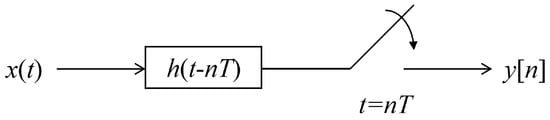
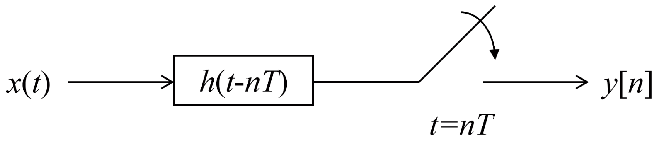
In the Classic FRI sampling structure as shown in Figure 1, the continuous-time signal $x\left(t\right)$ is typically passed through an analog pre-filter, characterized by a sampling kernel $h\left(t\right)$, before being digitized by an ADC. The filtered signal $y\left(t\right)$ is given by the convolution

$$y\left(t\right)=(x\ast h)\left(t\right)={\int }_{-\infty }^{\infty }x\left(s\right)h(t-s)ds.$$

(3)

Figure 1. The Classic FRI sampling structure.

Uniform sampling of $y\left(t\right)$ at a rate $f_s=1/T_s$ yields the discrete measurements

$$y\left[k\right]=y\left(k{T}_s\right)=⟨x\left(t\right),\phi (t-k{T}_s)⟩,n=0,\dots ,N-1,$$

(4)

where <·> denotes the inner product, and $\phi \left(t\right)=h(-t)$ denotes the effective sensing function and N is the total number of samples collected within one period $\tau$.

The classical FRI reconstruction strategy exploits the relationship between the time-domain samples $y\left[k\right]$ and the Fourier series coefficients of the periodic signal $x\left(t\right)$. Since $x\left(t\right)$ is $\tau$-periodic, it admits the Fourier series expansion

$$x\left(t\right)=\sum _{m\in \mathbb{Z}}\widehat{x}\left[m\right]e^{j2\pi mt/\tau },$$

(5)

where the Fourier coefficients $\widehat{x}\left[m\right]$ are given by

$$\widehat{x}\left[m\right]={\displaystyle \frac{1}{\tau }}\sum _{l=1}^L{a}_l{e}^{-j2\pi m{t}_l/\tau }.$$

(6)

Equation (6) reveals that the Fourier coefficients form a power sum of complex exponentials, a structure that constitutes the cornerstone of classical spectral estimation. This representation enables the use of AF techniques or subspace-based algorithms to recover the unknown sets $\left\{t_l\right\}$ and $\left\{a_l\right\}$.

However, as discussed in Section 1, the reliance on complex-valued Fourier bases introduces redundancy and numerical sensitivity when processing inherently real-valued physical signals. The key challenge addressed in this work is to reformulate the sampling-reconstruction paradigm by mapping the signal $x\left(t\right)$ onto a real-domain, numerically stable basis, namely, Chebyshev polynomials, while preserving the sub-Nyquist sampling property $N/\tau \ll f_{\mathrm{Nyquist}}$.

2.2. Chebyshev Polynomial

Chebyshev polynomials of the first kind, denoted as $T_k\left(t\right)$, are a sequence of orthogonal polynomials that play a central role in approximation theory and numerical analysis. Unlike the complex exponential bases used in Fourier analysis, Chebyshev polynomials are specifically tailored for real-valued functions defined on a closed interval. They are defined by the following three-term recurrence relation:

$$T_0\left(t\right)=1$$

(7)

$$T_1\left(t\right)=t$$

(8)

$$T_k\left(t\right)=2t{T}_{k-1}\left(t\right)-T_{k-2}\left(t\right),k\ge 2$$

(9)

where the independent variable t is typically restricted to the domain $t\in [-1,1]$. This recursive structure allows for the efficient and numerically stable computation of higher-order polynomials, a property that is particularly desirable for hardware-level signal processing.

One of the most profound characteristics of the Chebyshev polynomial $T_k\left(t\right)$ is its relationship with trigonometric functions. By performing a change of variable $t=cos\left(\theta \right)$, the polynomial admits the closed-form representation

$$T_k\left(t\right)=cos\left(karccos\left(t\right)\right),t\in [-1,1].$$

(10)

From (10), it follows immediately that

$$|T_k\left(t\right)|\le 1,\forall t\in [-1,1].$$

(11)

The roots of $T_k\left(t\right)$, known as Chebyshev nodes, are given by

$$t_i=cos\left({\displaystyle \frac{2i-1}{2k}}\pi \right),i=1,2,\dots ,k.$$

(12)

where k denotes the polynomial degree, and the k Chebyshev nodes are the roots of $T_k\left(t\right)$. These nodes cluster toward the endpoints of the interval and play a crucial role in mitigating Runge’s phenomenon, yielding superior numerical stability compared to uniform sampling.

The Chebyshev polynomials form a complete orthogonal basis for the weighted $L_2$ space

$$L_2([-1,1],\omega \left(t\right)),$$

(13)

with the weight function

$$\omega \left(t\right)={\displaystyle \frac{1}{\sqrt{1-t^2}}}.$$

(14)

The orthogonality condition is expressed as

$${\int }_{-1}^1{T}_l\left(t\right)T_m\left(t\right){\displaystyle \frac{dt}{\sqrt{1-t^2}}}={\alpha }_m{\delta }_{l,m},$$

(15)

where ${\delta }_{l,m}$ denotes the Kronecker delta, and the normalization constant ${\alpha }_m$ is given by

$${\alpha }_m=\left\{\begin{array}{cc}\pi ,\hfill & m=0,\hfill \\ {\displaystyle \frac{\pi }{2}},\hfill & m>0.\hfill \end{array}\right.$$

(16)

Given this orthogonal basis, any square-integrable function $h\left(t\right)$ defined on $[-1,1]$ can be represented by a convergent Chebyshev series

$$h\left(t\right)={\displaystyle \frac{1}{2}}{c}_0+\sum _{k=1}^{\infty }{c}_k{T}_k\left(t\right).$$

(17)

The expansion coefficients $c_k$ are obtained via orthogonal projection:

$$c_k={\displaystyle \frac{2}{\pi }}{\int }_{-1}^{1}h\left(t\right)T_k\left(t\right){\displaystyle \frac{1}{\sqrt{1-t^2}}}dt.$$

(18)

In conventional FRI sampling, a $\tau$-periodic signal $x\left(t\right)$ is expanded using a Fourier series. For a stream of L Dirac pulses, the Fourier coefficients are given by

$$X\left[k\right]={\displaystyle \frac{1}{\tau }}{\int }_0^{\tau }x\left(t\right)e^{-j{\displaystyle \frac{2\pi }{\tau }}kt}dt={\displaystyle \frac{1}{\tau }}\sum _{l=1}^L{a}_l{e}^{-j{\displaystyle \frac{2\pi }{\tau }}k{t}_l}.$$

(19)

The corresponding signal reconstruction formula is

$$x\left(t\right)=\sum _{k\in \mathbb{Z}}X\left[k\right]e^{j{\displaystyle \frac{2\pi }{\tau }}kt}.$$

(20)

By comparing the Chebyshev expansion in (17) with the Fourier expansion, several fundamental differences emerge. First, Fourier bases inherently impose periodic boundary conditions, which can lead to Gibbs artifacts when signals are observed over finite, non-periodic intervals. In contrast, Chebyshev polynomials do not enforce periodicity, making them more suitable for localized signal representations. Second, while Fourier bases rely on complex-valued exponentials, Chebyshev polynomials are purely real-valued, aligning naturally with physical sensor measurements and eliminating unnecessary complex-domain representations. Finally, the minimax property of Chebyshev polynomials ensures that approximation errors are more uniformly distributed across the interval, thereby improving numerical robustness and parameter recovery performance in FRI sampling systems.

3. FRI Sampling with Chebyshev Polynomials

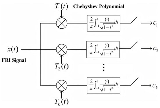
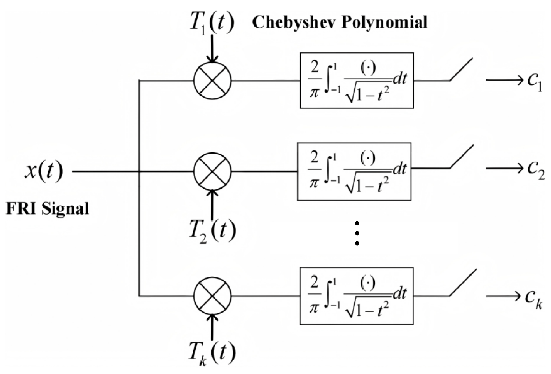
In this section, we consider the FRI sampling framework with Chebyshev polynomials. The modulation signals $T_k\left(t\right)$ in each channel are generated iteratively using the three-term recurrence

$$T_k\left(t\right)=2t{T}_{k-1}\left(t\right)-T_{k-2}\left(t\right),$$

(21)

initialized with $T_0\left(t\right)=1$ and $T_1\left(t\right)=t$. This recurrence maps directly to analog hardware, requiring only two multipliers and one adder per stage. Consequently, the architecture in Figure 2 requires no pre-designed sampling kernels, as each channel generates its modulation signal on the fly. This significantly reduces hardware complexity and eliminates the need for kernel calibration compared to classical Sum-of-Sincs or Dirichlet kernel architectures. When getting the sampling coefficients, we replace the Fourier basis with Chebyshev polynomials. We still use the signals like (1) but only focus on its single period. Without loss of generality, we assume the time delays $t_l\in [-1,1]$, for $l=0,\dots ,L-1$. The Chebyshev coefficient $c_k$ is computed by

$$\begin{array}{cc}\hfill c_k& ={\displaystyle \frac{2}{\pi }}{\int }_{-1}^1{T}_k\left(t\right)\sum _{l=1}^L{a}_l\delta (t-t_l){\displaystyle \frac{1}{\sqrt{1-t^2}}}dt\hfill \\ \hfill & ={\displaystyle \frac{2}{\pi }}\sum _{l=1}^L{a}_{l}cos\left(karccos{t}_l\right){\int }_{-1}^1\delta (t-t_l)dt\hfill \\ \hfill & ={\displaystyle \frac{2}{\pi }}\sum _{l=1}^L{a}_l{\displaystyle \frac{1}{\sqrt{1-t_l^2}}}cos\left(k{\theta }_l\right).\hfill \end{array}$$

(22)

Figure 2. The process of sampling Chebyshev polynomial coefficients.

The third equation holds because we let ${\theta }_l=arccos\left(t_l\right)$; hence, $t_l=cos\left({\theta }_l\right)$. The process of sampling Chebyshev polynomial coefficients is shown in Figure 2. We can observe that the modulation signal in each channel of this sampling architecture can be generated iteratively. Compared to the classical FRI sampling structure, it eliminates the need for sampling kernels, significantly reducing the system complexity and easing the calibration process. Because the starting point of time is zero, we generalize the integral from $-1$ to 1 by an affine function which is linear. To ensure that the input signal lies within the domain of Chebyshev polynomials, the time axis $\tau \in [a,b]$ is mapped to the interval $[-1,1]$ via the affine transformation as

$$t={\displaystyle \frac{2\tau -(a+b)}{b-a}},\tilde{x}\left(t\right)=x\left({\displaystyle \frac{(b-a)t+(a+b)}{2}}\right).$$

(23)

This transformation retains the signal’s structure while aligning it with the Chebyshev polynomial domain. The affine transformation can be implemented using analog circuits: (1) Time Scaling: A multiplier with gain $\alpha ={\displaystyle \frac{2}{b-a}}$; (2) Time Translation: An adder introducing offset $\beta =-{\displaystyle \frac{a+b}{b-a}}$.

3.1. Annihilating Filter Method

The recovery of the signal parameters ${\{t_l,a_l\}}_{l=1}^L$ from the sampled Chebyshev coefficients ${\left\{c_k\right\}}_{k=0}^M$ can be formulated as a high-resolution spectral estimation problem. In this section, we detail an improved AF method, specifically tailored to exploit the structural properties of real-valued Chebyshev-domain samples.

As derived in (22), the Chebyshev coefficients $c_k$ follow a sum-of-cosines structure. To apply the annihilating filter framework, which is traditionally designed for complex exponentials, Euler’s formula is employed to decompose the real-valued cosine terms. By defining

$${\theta }_l=arccos\left(t_l\right),$$

(24)

the coefficient $c_k$ can be rewritten as

$$\begin{array}{cc}\hfill c_k& ={\displaystyle \frac{1}{\pi }}\sum _{l=1}^L{\displaystyle \frac{a_l}{\sqrt{1-t_l^2}}}\left(e^{jk{\theta }_l}+e^{-jk{\theta }_l}\right)\hfill \\ \hfill & ={\displaystyle \frac{1}{\pi }}\sum _{l=1}^L{\tilde{a}}_l\left(e^{jk{\theta }_l}+e^{-jk{\theta }_l}\right),\hfill \end{array}$$

(25)

where

$${\tilde{a}}_l={\displaystyle \frac{a_l}{\sqrt{1-t_l^2}}}$$

(26)

denotes the modified amplitude.

Equation (25) reveals that each real-valued pulse in the Chebyshev domain is equivalent to a pair of complex conjugate exponentials located at $e^{\pm j{\theta }_l}$ on the unit circle. Consequently, the estimation of L real-valued delays $\left\{t_l\right\}$ is transformed into the problem of estimating the frequencies of $2L$ complex exponentials appearing in symmetric pairs.

The core of the AF method lies in constructing a filter $H\left(z\right)$ that annihilates the sequence $c_k$, i.e.,

$$c_k\ast h_k=0.$$

(27)

Since the roots of the filter must correspond to the complex exponentials $e^{\pm j{\theta }_l}$, the filter polynomial is defined as

$$H\left(z\right)=\prod _{l=1}^L\left(1-e^{j{\theta }_l}{z}^{-1}\right)\left(1-e^{-j{\theta }_l}{z}^{-1}\right)=\sum _{k=0}^{2L}{h}_k{z}^{-k}.$$

(28)

Because the roots occur in complex conjugate pairs, the filter coefficients exhibit Hermitian (centro-) symmetry. For real-valued signals, this symmetry is expressed as

$$h_k=h_{2L-k},k=0,\dots ,L,$$

(29)

with boundary conditions

$$h_0=h_{2L}=1.$$

(30)

This symmetry reduces the number of independent unknowns from $2L$ to L, significantly improving numerical stability and reducing the minimum required number of samples from $4L$ to $3L$. In the standard complex-domain annihilating filter, the $2L$ complex exponentials $e^{(\pm j{\theta }_l)}$ yield a filter $H\left(z\right)$ of degree $2L$ with $2L-1$ free coefficients. Constructing an overdetermined Toeplitz system therefore requires at least $4L$ samples. In our Chebyshev setting, the roots appear in conjugate pairs, giving the Hermitian symmetry

$$h_k=h_{2L-k}.$$

(31)

This reduces the number of independent unknowns from $2L-1$ to L. The resulting Toeplitz-plus-Hankel matrix ${\mathbf{C}}_{\mathrm{sys}}$ can be fully populated using samples indexed from 0 to $3L-1$, so only $3L$ samples are needed to form a well-determined system—a reduction from $4L$ to $3L$.

By exploiting the convolutional annihilation property and the symmetry of $\left\{h_k\right\}$, a system of linear equations can be constructed. For a sequence of $3L$ samples $\{c_0,c_1,\dots ,c_{3L-1}\}$, the system can be written as

$${\mathbf{C}}_{\mathrm{sys}}\mathbf{h}=\mathbf{0},$$

(32)

where

$$\left[\begin{array}{ccccc}{c}_{2L}+c_0& c_{2L-1}+c_1& \dots & c_{L+1}+c_{L-1}& c_L\\ c_{2L+1}+c_1& c_{2L}+c_2& \dots & c_{L+2}+c_L& c_{L+1}\\ ⋮& ⋮& \ddots & ⋮& ⋮\\ c_{3L-1}+c_{L-1}& c_{3L-2}+c_L& \dots & c_{2L}+c_{2L-2}& c_{2L-1}\end{array}\right]\left[\begin{array}{c}1\\ h_1\\ ⋮\\ h_{L-1}\\ h_L\end{array}\right]=\mathbf{0}.$$

(33)

The matrix ${\mathbf{C}}_{\mathrm{sys}}$ exhibits a Toeplitz-plus-Hankel structure, which is commonly encountered in real-valued sinusoidal frequency estimation. The system can be solved using singular value decomposition (SVD) or the Levinson–Durbin recursion for improved computational efficiency.

Once the filter coefficients $\left\{h_k\right\}$ are obtained, the roots of the polynomial

$$P\left(z\right)=\sum _{k=0}^{2L}{h}_k{z}^k$$

(34)

are computed. In the ideal noise-free case, all $2L$ roots lie on the unit circle. In the presence of noise, radial deviations may occur, and thus a projection is applied:

$${\tilde{r}}_m={\displaystyle \frac{r_m}{|r_m|}},m=1,\dots ,2L.$$

(35)

Due to conjugate symmetry, only the L roots with non-negative imaginary parts are retained. The angular parameters are then extracted as

$${\theta }_l=\left|arg\left({\tilde{r}}_l\right)\right|,{\theta }_l\in [0,\pi ].$$

(36)

Finally, the time delays in the Chebyshev domain are recovered via

$$t_l=cos\left({\theta }_l\right).$$

(37)

3.2. Amplitude Reconstruction via Least Squares

With the delays $\left\{t_l\right\}$ estimated, the amplitudes $\left\{a_l\right\}$ remain unknown. For all observed coefficients $k=1,\dots ,M$, the system can be written as

$$\mathbf{c}=\mathbf{C}\mathbf{S}\mathbf{a}=\mathbf{V}\mathbf{a},$$

(38)

where

• $\mathbf{c}={[c_1,c_2,\dots ,c_M]}^T$ is the coefficient vector;
• $\mathbf{S}=\mathrm{diag}({\displaystyle \frac{\pi }{\sqrt{1-t_1^2}}},\dots ,{\displaystyle \frac{\pi }{\sqrt{1-t_L^2}}})$ is a scaling matrix accounting for the Chebyshev weight function;
• $\mathbf{C}\in {\mathbb{R}}^{M\times L}$ with $C_{k,l}=cos\left(k{\theta }_l\right)$ is the real-sinusoid basis matrix.

The amplitude vector

$$\mathbf{a}={[a_1,\dots ,a_L]}^T$$

(39)

is optimally recovered using the least-squares solution, and the notation ${(·)}^T$ denotes the matrix transpose.

$$\mathbf{a}={\left({\mathbf{V}}^T\mathbf{V}\right)}^{-1}{\mathbf{V}}^T\mathbf{c}.$$

(40)

This two-stage reconstruction framework enables accurate recovery of both the temporal locations and amplitudes of the original FRI signal.

3.3. Hilbert Transform Method

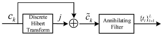
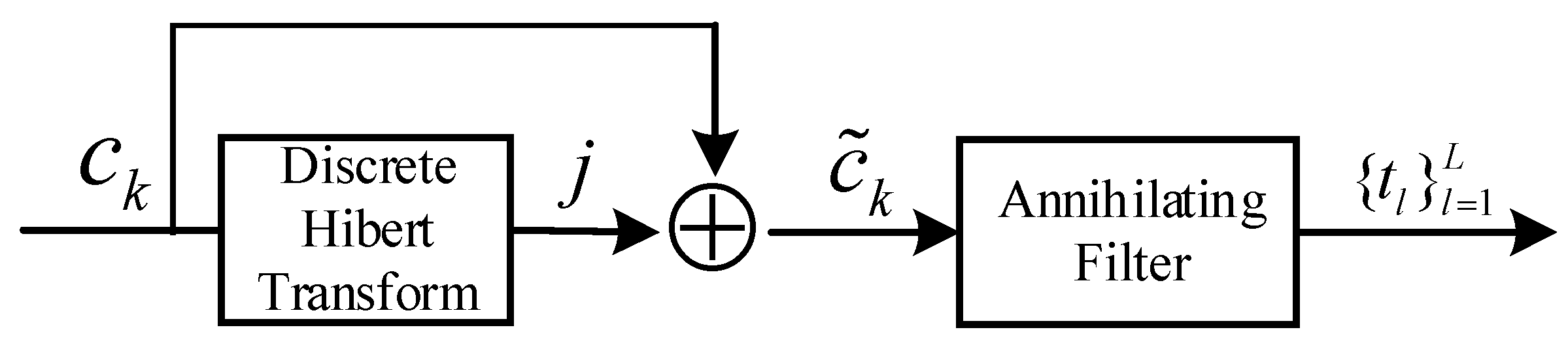
Although the annihilating filter method can obtain the exact solution, the order of the polynomials here is twice that of the complex signal. We propose to use the Hilbert transform to construct a complex signal from the real-sinusoid part as in (14). Let the discrete Hilbert transform operator be denoted by $\mathcal{H}$; then, the analytic signal ${\tilde{c}}_k$ is given as

$${\tilde{c}}_k=c_k+j\mathcal{H}\left(c_k\right)={\displaystyle \frac{2}{\pi }}\sum _{l=1}^L{a}_{l}sin\left({\theta }_l\right)e^{jk{\theta }_l}.$$

(41)

Therefore, we can estimate the parameters using the general annihilating filter method, which can be expressed as: $A\left(z\right)={\prod }_{l=1}^L\left(1-e^{j{\theta }_l}{z}^{-1}\right)={\sum }_{k=0}^L{a}_k{z}^{-k}$. Then, the time delays and amplitude parameters can be estimated using the method described in Section 3.1. We plot the algorithm flow in Figure 3. For the target applications of this work, such as short-range radar and ultrasonic imaging, signals are naturally acquired in finite-length bursts or frames, so the batch-processing assumption is fully compatible with the system architecture. We acknowledge that this limits applicability to strictly streaming systems. Future work could explore causal approximations of the Hilbert transform to enable near-online operation at the cost of a small bias.

Figure 3. Annihilating filter method based on Hilbert transform. j is the imaginary sign.

The dominant cost of the Chebyshev annihilating filter (AF) method lies in the singular value decomposition (SVD) of the $L\times L$ Toeplitz-plus-Hankel matrix ${\mathbf{C}}_{\mathrm{sys}}$, which has a complexity of $\mathcal{O}\left(L^3\right)$. The root-finding procedure for the degree-$2L$ polynomial $P\left(z\right)$ incurs a computational cost of $\mathcal{O}\left(L^2\right)$. For the Hilbert-transform-based variant, the polynomial order is reduced by half, which decreases the SVD complexity to $\mathcal{O}\left({(L/2)}^3\right)$.

For the classical FRI reconstruction framework, the signal is first low-pass filtered and uniformly sampled to obtain N low-frequency measurements. If the Fourier-series coefficients are recovered digitally through a DFT/FFT, this preprocessing step has complexity $\mathcal{O}(NlogN)$; if these coefficients are directly provided by the analog frontend, the corresponding digital cost is negligible. Then, the Prony method or annihilating-filter method constructs and solves a linear system of size approximately $L\times L$, whose computational complexity is typically $\mathcal{O}\left(L^3\right)$. After estimating the Lth-order annihilating filter, root-finding for the corresponding degree-L polynomial requires about $\mathcal{O}\left(L^2\right)$. Finally, the amplitudes are recovered by solving an $L\times L$ Vandermonde system, which also incurs a complexity of $\mathcal{O}\left(L^3\right)$. Therefore, the total complexity of the classical FRI method can be expressed as $\mathcal{O}(NlogN+L^3+L^2)$, which is typically dominated by $\mathcal{O}(NlogN+L^3)$. When N is on the order of L, the overall complexity can be approximated as $\mathcal{O}\left(L^3\right)$. Compared with the classical Fourier-based FRI scheme, whose complexity is typically $\mathcal{O}(NlogN+L^3)$ due to the DFT/FFT preprocessing and the subsequent Prony reconstruction, the proposed Chebyshev-domain method has a comparable asymptotic complexity but avoids the Fourier preprocessing stage and operates entirely in the real domain.

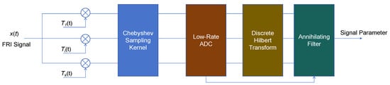
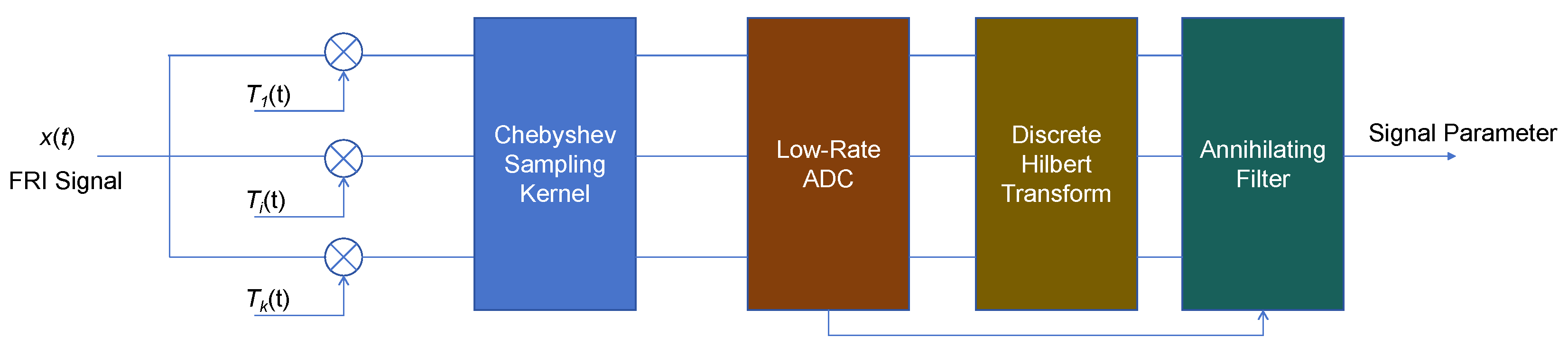
The complete processing pipeline of the proposed method is illustrated in Figure 4. The FRI signal $x\left(t\right)$ is simultaneously correlated with K Chebyshev sampling kernels ${\left\{T_k\left(t\right)\right\}}_{k=1}^K$, yielding the Chebyshev polynomial coefficients $\left\{c_k\right\}$. These coefficients are digitized by a low-rate ADC, and one of two reconstruction schemes is selected according to practical requirements. In the Hilbert transform scheme, a discrete Hilbert transform is applied to construct the analytic signal ${\tilde{c}}_k=c_k+j\mathcal{H}\left\{c_k\right\}$, converting the real cosine-sum model into a standard complex exponential form suitable for the classical annihilating filter, with only $N=2L$ samples required. In the direct scheme, the real-valued coefficients are fed directly into a modified annihilating filter that exploits the conjugate symmetry of $H\left(z\right)$, requiring $N=3L$ samples but avoiding the Hilbert transform entirely. Both schemes require far fewer samples than the Nyquist rate of the original signal. In either case, the polynomial roots of the annihilating filter yield the time delay estimates $\left\{{\widehat{t}}_l\right\}$, from which the amplitudes $\left\{{\widehat{a}}_l\right\}$ are recovered by least squares.

Figure 4. Block diagram of the proposed Chebyshev-based FRI sampling and reconstruction system.

To improve the noise robustness of the Chebyshev-domain reconstruction, two anti-noise algorithms are developed in this work, namely, the Cadzow + AF method and the Cadzow + ESPRIT method. Their common idea is to first exploit the structured low-rank property of the Chebyshev coefficient sequence to suppress noise, and then recover the delay parameters by using either annihilating filtering or subspace-based estimation.

Let the noisy Chebyshev coefficient sequence be denoted by

$${\tilde{c}}_k=c_k+n_k,k=0,1,\dots ,N-1,$$

where $n_k$ denotes additive noise. The Hankel matrix constructed from $\left\{c_k\right\}$ is ideally of rank $2L$, which provides the structural basis for noise suppression. For both proposed algorithms, the first step is Cadzow denoising. A Hankel matrix is formed from the noisy coefficients as

$$\mathbf{H}\left(\tilde{\mathbf{c}}\right)=\left[\begin{array}{cccc}{\tilde{c}}_0& {\tilde{c}}_1& \dots & {\tilde{c}}_p\\ {\tilde{c}}_1& {\tilde{c}}_2& \dots & {\tilde{c}}_{p+1}\\ ⋮& ⋮& \ddots & ⋮\\ {\tilde{c}}_{N-p-1}& {\tilde{c}}_{N-p}& \dots & {\tilde{c}}_{N-1}\end{array}\right].$$

Its singular value decomposition is written as

$$\mathbf{H}=\mathbf{U}\mathbf{\Sigma }{\mathbf{V}}^{\mathrm{H}}.$$

Then, only the largest $2L$ singular values are retained, yielding the rank-$2L$ approximation

$${\mathbf{H}}_{2L}=\mathbf{U}{\mathbf{\Sigma }}_{2L}{\mathbf{V}}^{\mathrm{H}},$$

where

$${\mathbf{\Sigma }}_{2L}=\mathrm{diag}({\sigma }_1,\dots ,{\sigma }_{2L},0,\dots ,0).$$

Finally, a denoised coefficient sequence ${\widehat{c}}_k$ is obtained by averaging the entries of ${\mathbf{H}}_{2L}$ along each anti-diagonal. This step projects the noisy data back onto the structured low-rank set implied by the underlying FRI model, thereby suppressing model-inconsistent noise components before parameter recovery.

The first anti-noise algorithm is the Cadzow + AF method. After Cadzow denoising, the cleaned coefficient sequence $\left\{{\widehat{c}}_k\right\}$ is substituted into the annihilating-filter model

$$P\left(z\right)=\prod _{\mathsf{\ell }=1}^L\left(1-e^{j{\theta }_{\mathsf{\ell }}}{z}^{-1}\right)\left(1-e^{-j{\theta }_{\mathsf{\ell }}}{z}^{-1}\right)=1+\sum _{m=1}^{2L-1}{h}_m{z}^{-m}+z^{-2L}.$$

Because the roots appear in conjugate pairs, the filter has a symmetric real-coefficient structure. The corresponding annihilation equations are assembled into a linear system, from which the filter coefficients are estimated. The delay parameters are then obtained from the phases of the roots located on the unit circle,

$${\widehat{t}}_{\mathsf{\ell }}=cos\left({\widehat{\theta }}_{\mathsf{\ell }}\right).$$

The advantage of this method is that it preserves the original annihilating-filter framework while significantly improving robustness through the structural denoising step.

The second anti-noise algorithm is the Cadzow + ESPRIT method. After the same Cadzow preprocessing, a denoised Hankel matrix is constructed, and its signal subspace is extracted by singular value decomposition. Let ${\mathbf{E}}_s$ denote the signal subspace associated with the largest $2L$ singular values. By partitioning it into two shifted submatrices,

$${\mathbf{E}}_{s,1}={\mathbf{E}}_s(1:end-1,:),{\mathbf{E}}_{s,2}={\mathbf{E}}_s(2:end,:),$$

the rotational invariance relation is exploited through

$$\mathbf{\Psi }={\mathbf{E}}_{s,1}^{†}{\mathbf{E}}_{s,2},$$

where ^† denotes the Moore–Penrose pseudoinverse. The eigenvalues of $\mathbf{\Psi }$ satisfy

$${\lambda }_{\mathsf{\ell }}\approx e^{\pm j{\theta }_{\mathsf{\ell }}},$$

and the delays are estimated as

$${\widehat{t}}_{\mathsf{\ell }}=cos\left(arg\left({\lambda }_{\mathsf{\ell }}\right)\right).$$

Compared with the annihilating-filter implementation, the ESPRIT-based estimator avoids direct high-order polynomial rooting and is therefore numerically more stable under noisy conditions.

After the delays are estimated by either method, the amplitudes are recovered by least squares. Specifically, the coefficient model can be written as

$$\widehat{\mathbf{c}}=\mathbf{C}(\widehat{\mathit{\theta }})\mathbf{S}(\widehat{\mathit{\theta }})\mathbf{a},$$

where

$${[\mathbf{C}(\widehat{\mathit{\theta }})]}_{k,\mathsf{\ell }}=cos(k{\widehat{\theta }}_{\mathsf{\ell }}),\mathbf{S}\left(\widehat{\mathit{\theta }}\right)=\mathrm{diag}\left({\displaystyle \frac{1}{sin{\widehat{\theta }}_1}},\dots ,{\displaystyle \frac{1}{sin{\widehat{\theta }}_L}}\right).$$

Hence, the amplitude vector is obtained by

$$\widehat{\mathbf{a}}=arg\underset{\mathbf{a}}{min}{∥\widehat{\mathbf{c}}-\mathbf{C}\left(\widehat{\mathit{\theta }}\right)\mathbf{S}\left(\widehat{\mathit{\theta }}\right)\mathbf{a}∥}_2^2.$$

In summary, the Cadzow + AF method improves the robustness of the original Chebyshev annihilating-filter framework by introducing structured low-rank denoising, while the Cadzow + ESPRIT method further enhances the stability by replacing polynomial rooting with subspace-based rotational-invariance estimation.

4. Super-Resolution Properties and Resolution Amplification

A defining characteristic of the proposed Chebyshev-based FRI framework is its ability to achieve super-resolution, particularly for pulses located near the boundaries of the observation interval. While traditional FRI is “grid-free,” it is not immune to the ill-conditioning that occurs when pulses are spaced more closely than the main lobe of the sampling kernel. In this section, we provide a rigorous analysis of how the non-linear nature of Chebyshev polynomials enhances the resolvability of closely spaced innovations.

4.1. Non-Linear Mapping and Resolution Amplification

The core of Chebyshev super-resolution lies in the non-linear warping of the time axis. When referring to the l-th pulse specifically, As established in (22), the time delays $t_l$ are mapped to the angular domain via

$${\theta }_l=arccos\left(t_l\right).$$

(42)

To understand how this affects resolution, we examine the sensitivity of the angular parameter $\theta$ with respect to the temporal parameter t. The differential relationship is given by

$${\displaystyle \frac{d\theta }{dt}}=-{\displaystyle \frac{1}{\sqrt{1-t^2}}},t\in (-1,1).$$

(43)

Consider two Dirac pulses separated by a minute temporal distance $\Delta t$ at a centered location t. The resulting separation in the angular domain, $\Delta \theta$, can be approximated using a first-order Taylor expansion:

$$\Delta \theta \approx \left|{\displaystyle \frac{d\theta }{dt}}\right|\Delta t={\displaystyle \frac{\Delta t}{\sqrt{1-t^2}}}.$$

(44)

We define the Resolution Amplification Factor (RAF) as

$$A\left(t\right)={(1-t^2)}^{-1/2}.$$

(45)

The behavior of $A\left(t\right)$ reveals a position-dependent resolution characteristic:

• Center Region ($t\approx 0$): In this case, $A\left(t\right)\approx 1$ and $\Delta \theta \approx \Delta t$. The mapping is quasi-linear, and the resolution is comparable to that of standard spectral estimation.
• Boundary Regions ($t\to \pm 1$): As the pulses approach the boundaries, $A\left(t\right)\to \infty$. This implies that a vanishingly small separation in the time domain $\Delta t$ is stretched into a significant separation $\Delta \theta$ in the angular domain. This stretching effect effectively pushes the complex conjugate roots $e^{\pm j\theta }$ further apart on the unit circle, making them significantly easier for the annihilating filter to distinguish.

4.2. Local Frequency Analysis and the Resolution Limit

The resolving power can also be interpreted through the lens of the local instantaneous frequency of the Chebyshev basis. The k-th order Chebyshev polynomial

$$T_k\left(t\right)=cos\left(karccost\right)$$

(46)

oscillates more rapidly near the edges of the interval $[-1,1]$. Its local frequency $f_{\mathrm{local}}\left(t\right)$ is derived as

$$f_{\mathrm{local}}\left(t\right)={\displaystyle \frac{1}{2\pi }}\left|{\displaystyle \frac{d}{dt}}\left(karccost\right)\right|={\displaystyle \frac{k}{2\pi \sqrt{1-t^2}}}.$$

(47)

The number of oscillations captured within a small interval $\Delta t$ is given by

$$N_{\mathrm{osc}}(t,\Delta t)={\int }_t^{t+\Delta t}{\displaystyle \frac{k}{2\pi \sqrt{1-s^2}}}ds\approx {\displaystyle \frac{k\Delta t}{2\pi \sqrt{1-t^2}}}.$$

(48)

According to a Rayleigh-like criterion for parametric estimation, two pulses are resolvable if the sampling basis captures at least a certain fraction of an oscillation cycle between them. By setting the threshold $N_{\mathrm{osc}}\ge \gamma$, where $\gamma$ is a dimensionless threshold analogous to the Rayleigh resolution criterion. It captures the minimum number of Chebyshev basis oscillation cycles required between two pulses for reliable resolution. In general, $\gamma$ does not admit a closed-form solution, as it depends on the SNR. In practice, a conservative choice of $\gamma =1$ is commonly adopted, which requires at least one full oscillation cycle of the k-th Chebyshev polynomial between the two pulses. The minimum resolvable time separation $\Delta t_{min}$ satisfies

$$\Delta t_{min}\left(t\right)\approx {\displaystyle \frac{2\pi \gamma \sqrt{1-t^2}}{k}}.$$

(49)

Equation (49) quantitatively demonstrates that by increasing the number of sampled coefficients k, or by exploiting the natural “stretching” near $t=\pm 1$, the system can resolve pulses that would otherwise be inseparable in a linear sampling framework. Then, we compared the proposed methods with the classical Fourier-FRI approach as shown in Table 1.

Table 1. Comparison of sampling requirements for different methods.

Method	Domain	Min. Samples	Channels
Fourier-FRI (standard AF)	Complex	$2L$	1
Chebyshev AF (proposed)	Real	$3L$	$3L$
Chebyshev + Hilbert (proposed)	Real	$2L$	$2L$

4.3. Comparison with Classical FRI Bottlenecks

In contrast, classical FRI sampling frameworks based on sinc or Dirichlet kernels are shift-invariant, meaning their resolution is uniform across the time axis and strictly limited by the kernel bandwidth.

When two Dirac pulses located at $t_1$ and $t_2$ are extremely close, classical FRI systems suffer from two fundamental limitations:

1.

Kernel Blurring: The observed signal

$$y\left(t\right)=\sum _l{a}_{l}h(t-t_l)$$

(50)

is a convolution in which the Dirac pulses are replaced by overlapping kernel responses. If $\Delta t=|t_1-t_2|$ is much smaller than the main-lobe width of $h\left(t\right)$, the pulses merge into a single peak, and the Fisher information associated with their individual delays drops sharply [8,10].

2.

Numerical Rank Deficiency: In the Fourier domain, the annihilating filter relies on a Toeplitz matrix constructed from exponentials $e^{-j\omega t_l}$. As $t_1\to t_2$, the columns of the corresponding Vandermonde matrix become nearly linearly dependent, leading to an extremely large condition number and making root-finding highly sensitive to even infinitesimal noise perturbations [33,34].

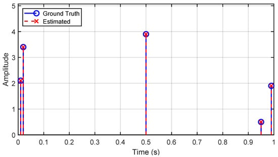
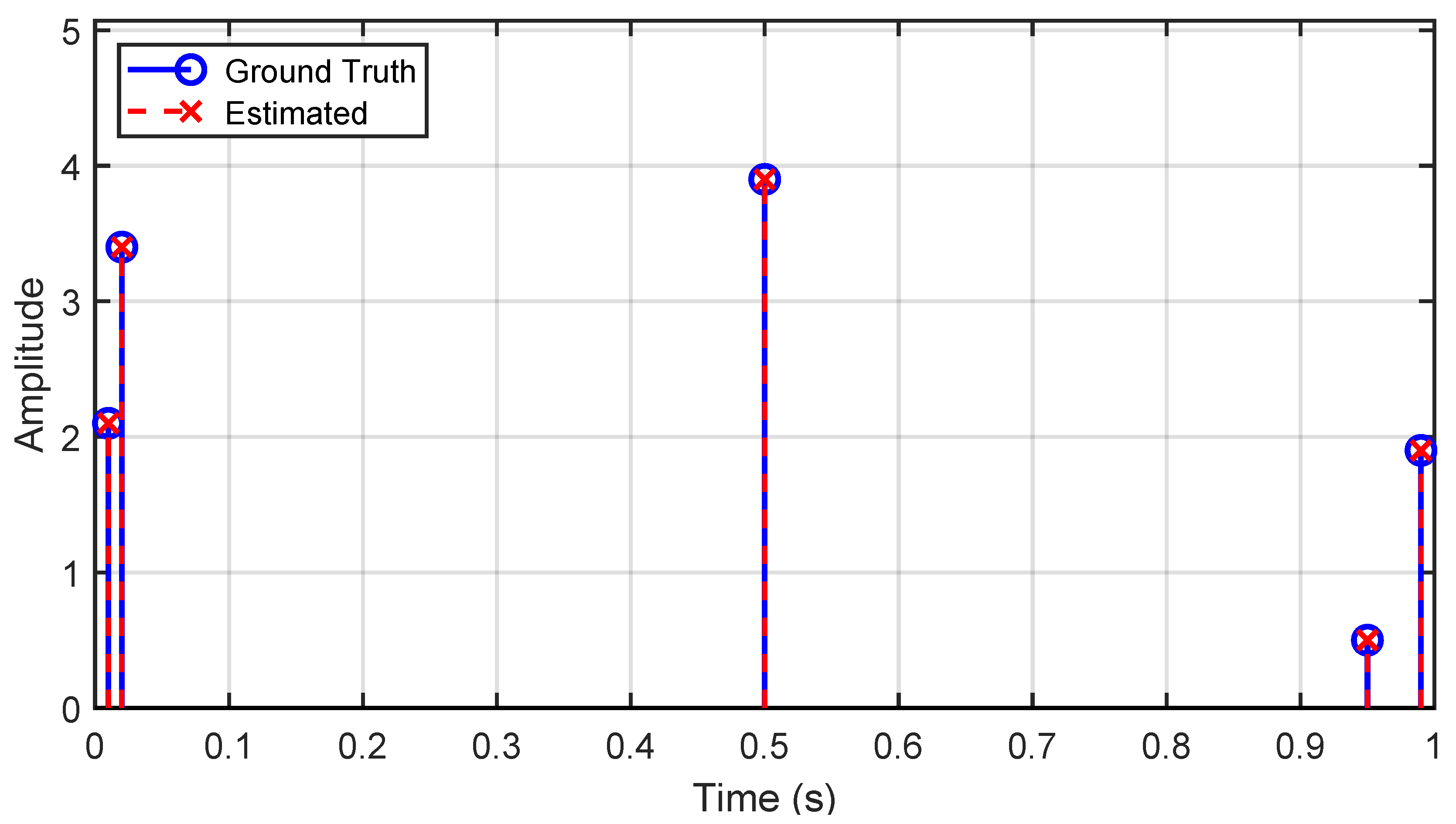
The proposed Chebyshev framework bypasses these limitations by non-linearly increasing the effective sampling density near the boundaries and by maintaining a real-valued symmetric matrix structure. Consequently, the Chebyshev-domain annihilating filter remains well-conditioned even when $\Delta t$ is small, providing a solid theoretical foundation for ultra-high-precision applications such as short-range radar and high-resolution ultrasonic imaging. As shown in Figure 5, the proposed method successfully recovers all five pulses, including the closely spaced pair near $t=0.02$ s, with negligible error in both time delay and amplitude, confirming the numerical stability of the reconstruction even for closely spaced pulses.

Figure 5. Reconstruction of a Dirac pulse stream containing two closely spaced pulses (separation $\Delta t=0.02$ s) and three well-separated pulses.

5. Numerical Simulation Results

In this section, we present some numerical simulation results to validate the algorithms we proposed. The signal under consideration is a Dirac pulse stream.

We first consider the noiseless case. The amplitude parameters are assumed as ${\mathbf{a}}_l=[2.1,3.4,1.7,0.5,1.9]$ and the time delay parameters are all included in $[0,1]$:$t_l=[0.13,0.35,0.47,0.64,0.82].$ The number of Chebyshev coefficients is $3L=15$. As shown in Figure 6, we are able to reconstruct the original signal exactly in the noiseless case. The sampling rate of our method is much lower than the bandwidth of the original signal. For the simulation with $L=5$ Dirac pulses over the interval $[0,1]$, the rate of innovation is given by

$$\rho ={\displaystyle \frac{2L}{\tau }}=10\mathrm{parameters}\mathrm{per}\mathrm{second}.$$

(51)

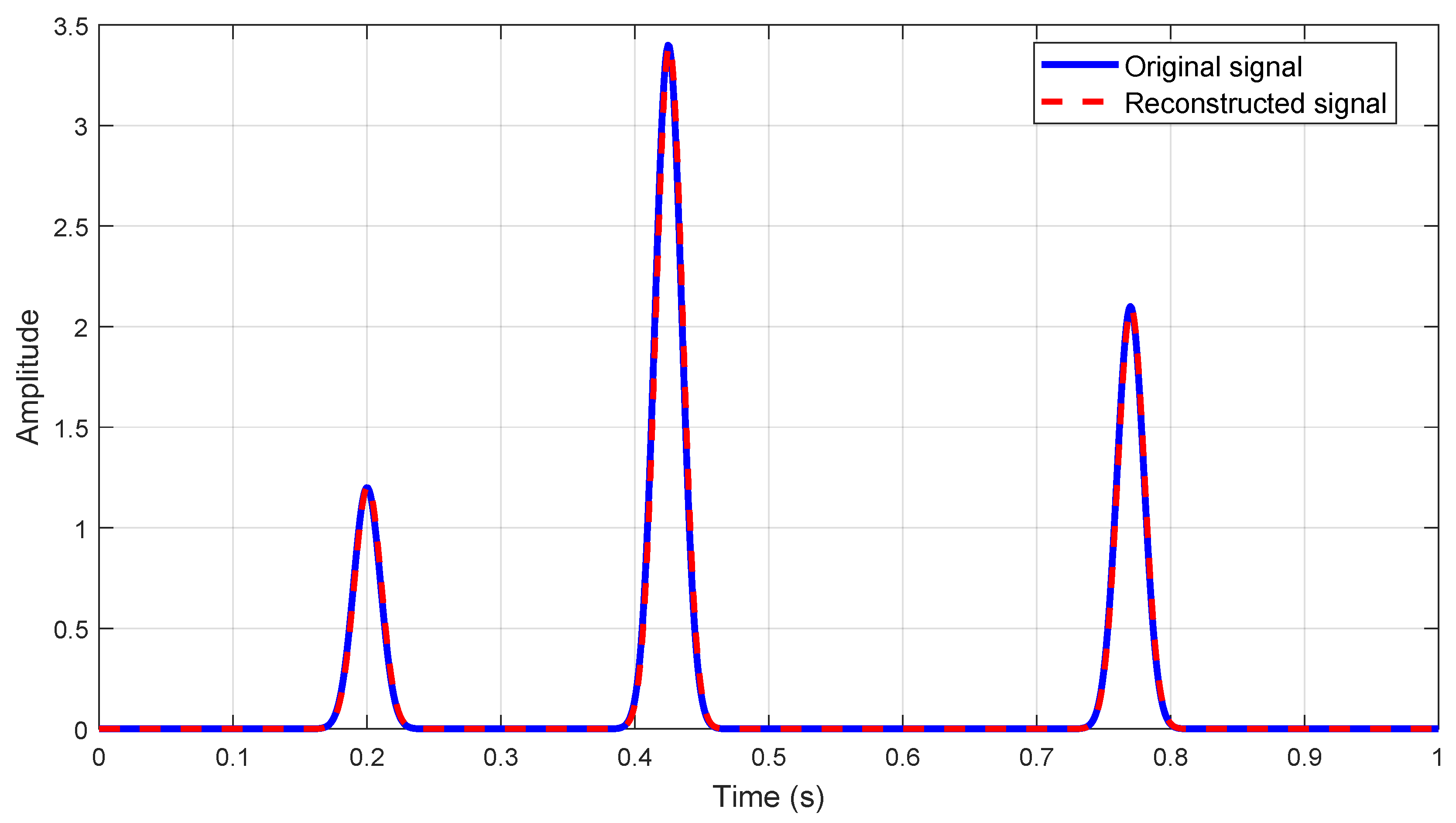
The proposed method uses only $N=3L=15$ Chebyshev coefficients per period. In contrast, the Nyquist rate for a stream of Dirac pulses is theoretically infinite. The effective sampling rate of the proposed method equals the rate of innovation $\rho$, which is fully consistent with FRI theory. Furthermore, the capability of the proposed method for recovering more general signals was also validated. In this experiment, three Gaussian pulses were considered, whose amplitudes, time delays, and standard deviation were set as $a=[2.1,3.4,1.2],$ $t=[0.77,0.425,0.2],$ and ${\sigma }_t=0.01$. As illustrated in Figure 7, the proposed method can accurately recover the original signal.

Figure 6. FRI–Chebyshev Polynomial method. The blue line is the original signal, and the red dotted line is the reconstructed signal.

Figure 6. FRI–Chebyshev Polynomial method. The blue line is the original signal, and the red dotted line is the reconstructed signal.

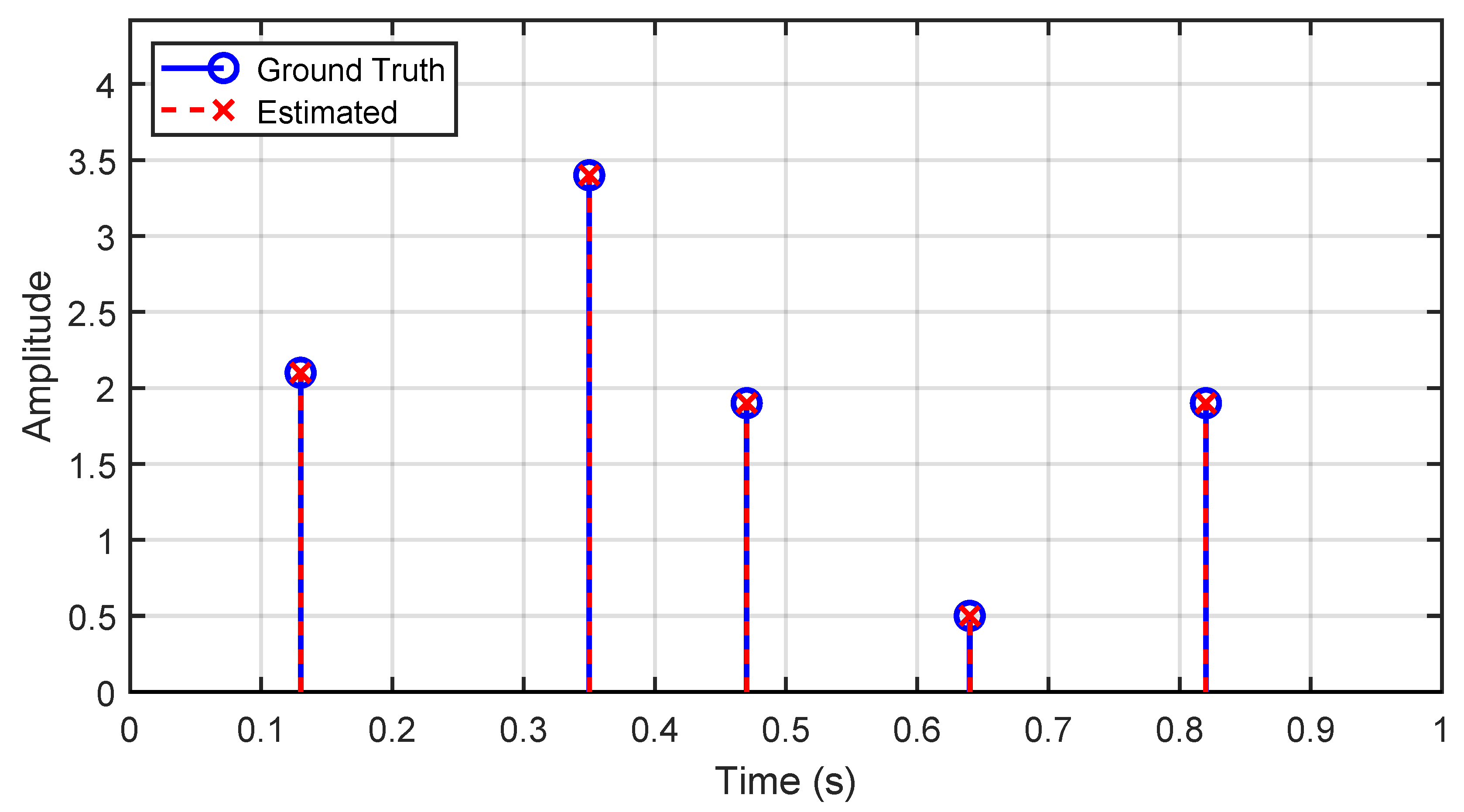
Figure 7. Reconstruction of the Gaussian pulse using the Chebyshev sampling architecture.

Figure 7. Reconstruction of the Gaussian pulse using the Chebyshev sampling architecture.

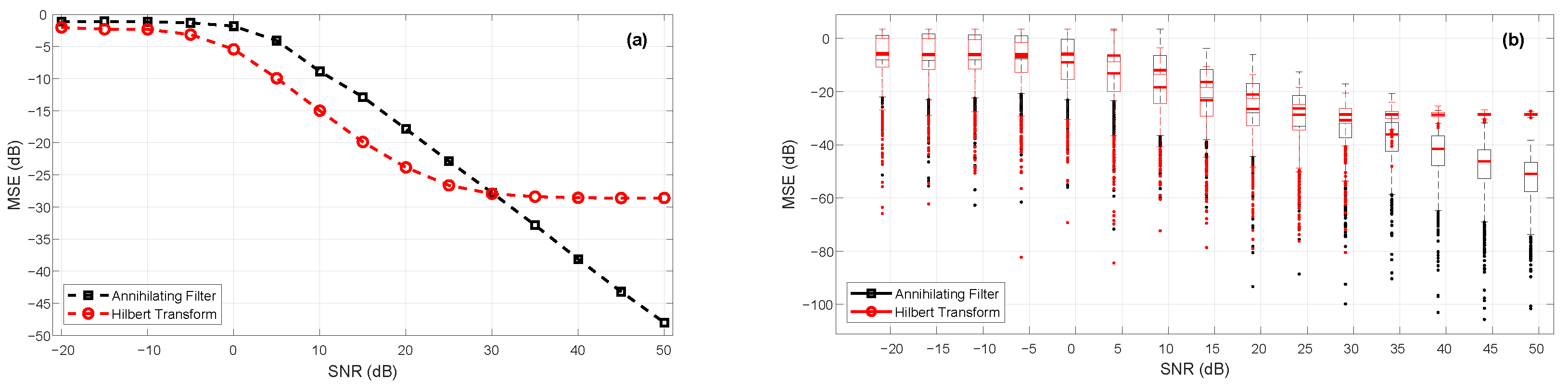
Next, we add noise with different SNRs to the original signal. In this experiment, all results were obtained by averaging over 500 independent Monte Carlo simulations. The number of data samples was $N=15$. The red dotted line represents the Hilbert transform method, while the other line represents the Annihilating filter method. The statistical contrast between the two methods is striking. At relatively low SNR, the Hilbert transform method is statistically superior to the annihilating filter method. This phenomenon occurs because the annihilating method requires at least $3L$ sample values to estimate the parameters. When these sample values are disturbed by noise, more data are required to obtain the same amount of information as compared to the annihilating filter. The MSE saturation observed in the Hilbert Transform method at high SNR is caused by the finite-length discrete Hilbert transform (DHT). For a fixed sequence length N, the DHT introduces a deterministic approximation error that is independent of the noise level. As the SNR increases, the noise eventually falls below this error floor, preventing any further reduction in MSE.

In theory, the Hilbert transform of a cosine signal yields its sine pair. However, the accuracy of the transformation depends on the amount of data. Suppose the transformation is applied to an analog signal: the output of the system would be perfect. In practice, our goal is to reconstruct the original signal from a small set of samples. Whether noise is present or not, errors arise when estimating the imaginary part from the Hilbert transform of a small sample set. Figure 8 validates this assumption.

Figure 8. Comparison of MSE of the Annihilating Filter and Hilbert Transform methods on the FRI signal. The number of sample elements is $N=15$. (a) Mean MSE curves averaged over 500 Monte Carlo trials. (b) Box plots showing the statistical distribution of MSE across 500 Monte Carlo trials, where the box represents the interquartile range (IQR), the central line denotes the median, the whiskers extend to 1.5 times the IQR, and the dots indicate outliers.

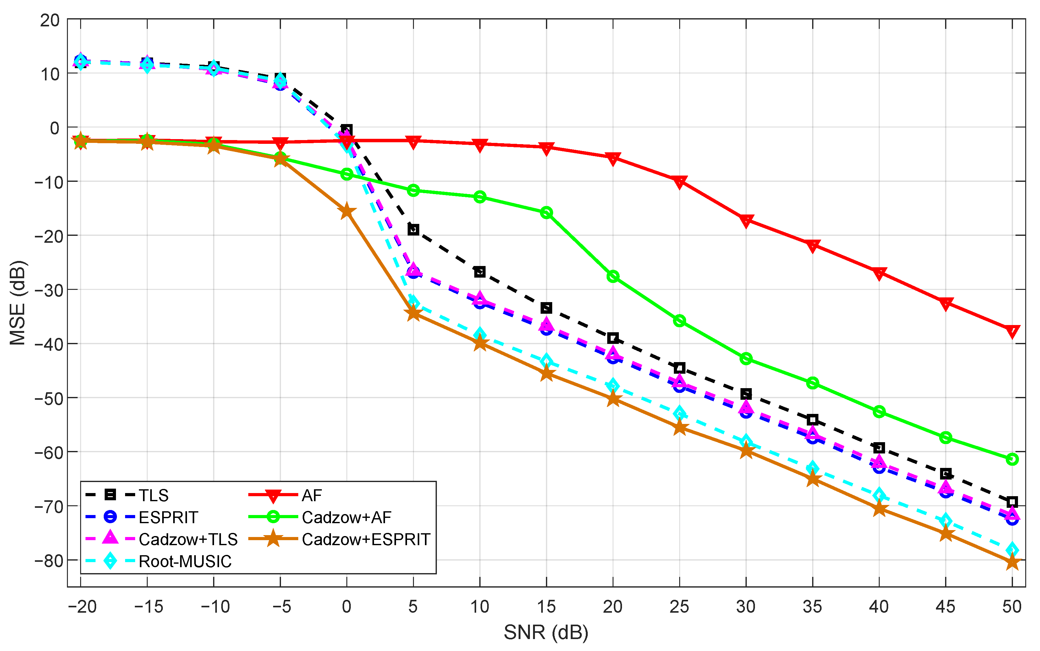
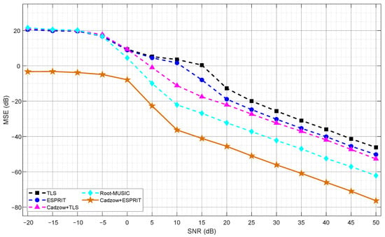
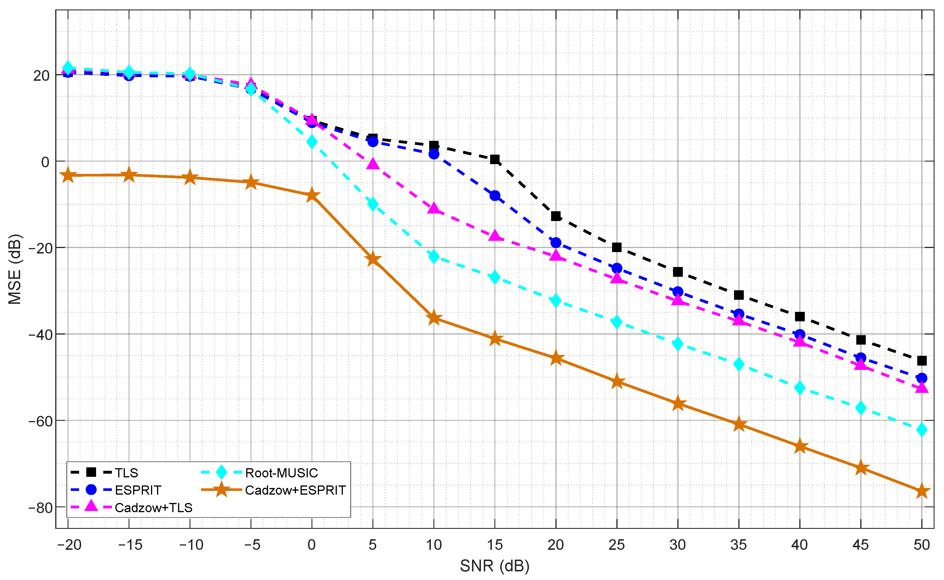
Then, Figure 9 considers a single Dirac pulse located near the boundary of the observation window. The solid lines represent the three solution methods based on the Chebyshev sampling kernel, while the dashed lines represent the four classical FRI sampling and reconstruction methods: TlS [12], ESPRIT [10], Cadzow [8] and Root-MUSIC [22]. The experiment considers a single Dirac pulse located at $t_1=0.1$ s with unit amplitude $a_1=1$. All methods use $N=27$ samples, and all results are averaged over 500 independent Monte Carlo trials across the SNR range of $-20$ to 50 dB. In this setting, the proposed Cadzow + ESPRIT method consistently achieves the lowest MSE over the entire SNR range. Unlike the classical Fourier-domain baselines, the proposed method operates in the Chebyshev domain, where the nonlinear mapping

$$\theta =arccos\left(t\right)$$

increases the local sensitivity of the coefficient sequence to the pulse location near the boundaries. As a result, the delay parameter becomes easier to estimate in the transformed domain. While the plain AF method is still highly sensitive to noise because of its direct polynomial-rooting step, the combination of Cadzow denoising and ESPRIT fully exploits the low-rank structure and the rotational invariance of the denoised signal subspace. This explains why the proposed method outperforms both the classical Fourier-domain baselines and the weaker Chebyshev-domain variants throughout the full SNR range.

Figure 9. MSE comparison of the proposed methods and classical baselines as a function of SNR, averaged over 500 Monte Carlo trials.

Figure 10 considers an extremely challenging case with two closely spaced Dirac pulses located near the boundary of the observation window ($t_1=0.02$ s and $t_2=0.12$ s) and $N=27$ samples. In this setting, the proposed Cadzow + ESPRIT method consistently achieves the lowest MSE over the entire SNR range. This superiority stems from two aspects. On the one hand, the Chebyshev mapping amplifies small temporal separations near the boundaries into larger angular separations, thereby improving the intrinsic resolvability of closely spaced pulses. On the other hand, the combination of Cadzow denoising and ESPRIT estimation further enhances the robustness by exploiting the low-rank structure of the coefficient sequence and avoiding unstable direct polynomial rooting. In contrast, the classical Fourier-domain baselines remain limited by shift-invariant resolution and by the ill-conditioning of the Fourier-domain Vandermonde structure in the closely spaced regime.

Figure 10. Time-delay estimation accuracy for closely spaced pulses. Two Dirac pulses are located near the boundary of the observation window ($t_1=0.02$ s, $t_2=0.12$ s) with a separation of $0.1$ s.

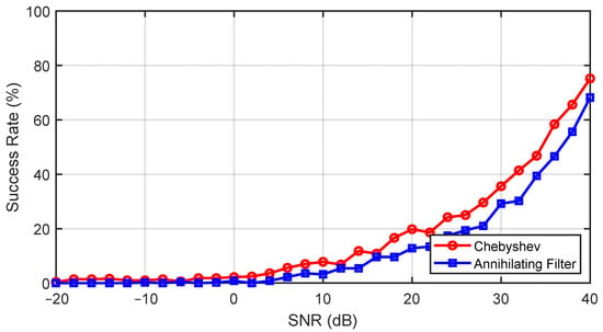
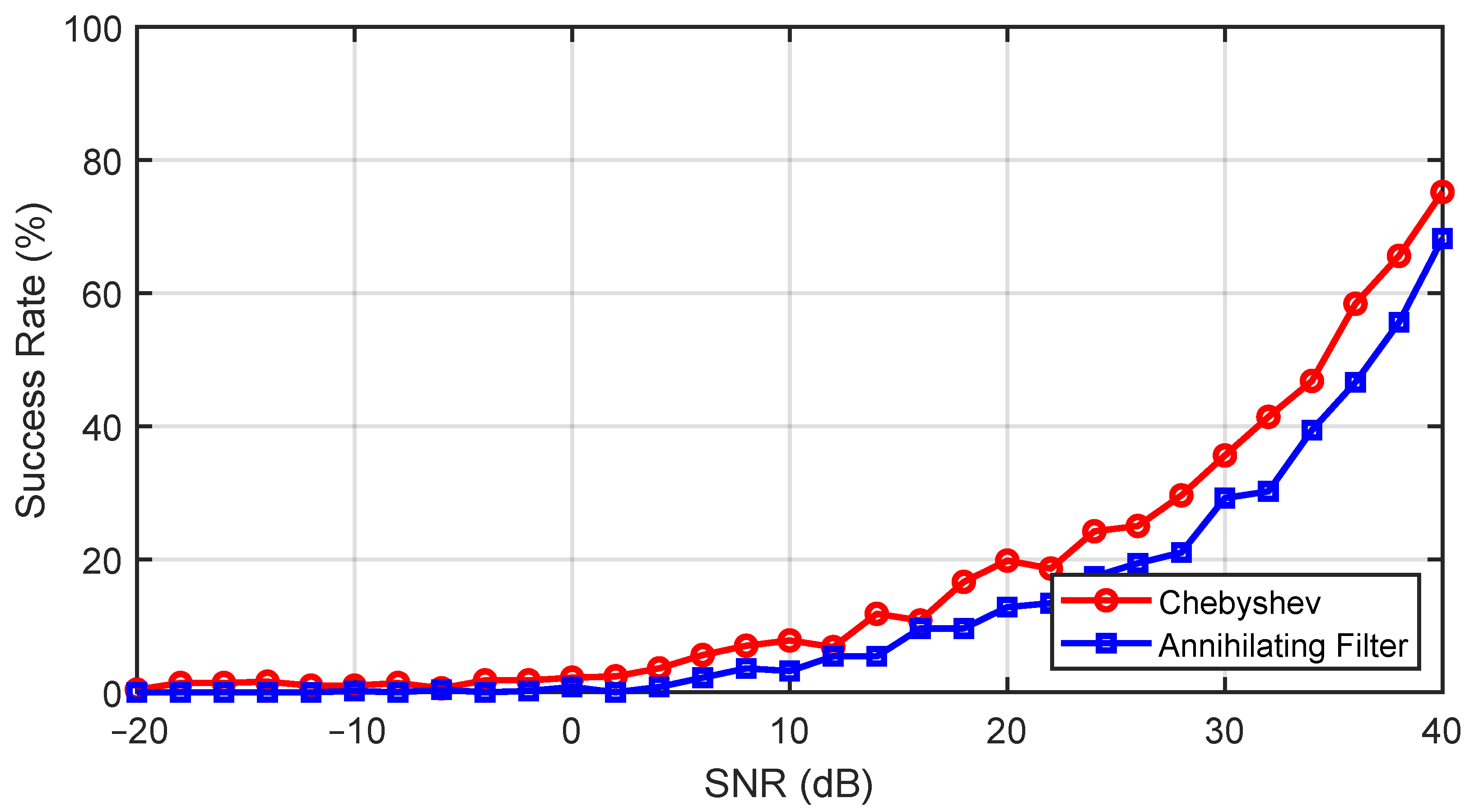
Furthermore, we select one pulse delay located close to the boundary of the time window. In this case, due to the bandwidth expansion effect of the filter, part of the signal information may be directly suppressed, thereby degrading the recovery performance. In contrast, as revealed by the previous analysis, the proposed method exhibits enhanced resolution capability when the pulse is located near the time-window boundaries. This experiment is therefore conducted to validate the advantage of the proposed method over the classical FRI annihilating filter approach. We define a successful recovery as the case where the estimation error of the time delay is less than 0.01 s. The detailed results are shown in Figure 11.

Figure 11. Success rate of pulse recovery near the time-window boundaries.

It can be observed that, due to the enhanced resolution capability, the proposed method achieves superior reconstruction performance compared with the conventional approach, which further demonstrates the potential of the proposed method.

6. Conclusions

We extend the classical FRI framework using Chebyshev polynomials. By projecting FRI signals onto the Chebyshev basis, the characteristic parameters are embedded in the polynomial coefficients, enabling accurate reconstruction via the annihilating filter. A Hilbert transform-based strategy further reduces the required number of samples from $3L$ to $2L$, at the cost of an MSE saturation floor at high SNR induced by the finite-length discrete Hilbert transform. Additionally, the proposed method assumes that the pulse number L and the signal period $\tau$ are known a priori, which may limit its applicability in practice. Potential application scenarios include radar, sonar, and medical ultrasound imaging, where sub-Nyquist acquisition of pulse streams is highly desirable. Incorporating robust preprocessing such as Cadzow denoising to further improve noise resilience remains an important direction for future work.

References

- Shannon, C. Communication in the Presence of Noise. Proc. IRE 1949, 37, 10–21. [Google Scholar] [CrossRef] [Scilit]
- Xiao, S.; Wei, Y.; Yue, W.; Sun, C.; Wang, S.; Tian, A.; Mi, S.; Cao, J. Pilot Design for Block Compressed Sensing-Based MIMO-OFDM Channel Estimation with Joint Criterion. Electronics 2025, 14, 4262. [Google Scholar] [CrossRef] [Scilit]
- Nyquist, H. Certain Topics in Telegraph Transmission Theory. Trans. AIEE 1928, 47, 617–644. [Google Scholar] [CrossRef] [Scilit]
- Unser, M. Sampling-50 years after Shannon. Proc. IEEE 2000, 88, 569–587. [Google Scholar] [CrossRef] [Scilit]
- Jiang, S.; Wei, Z.; Fu, N.; Qiao, L.; Peng, X. Sub-Nyquist Frequency and DOA Estimation with DOF Extension Arrayed MWC. IEEE Signal Process. Lett. 2024, 31, 1645–1649. [Google Scholar] [CrossRef] [Scilit]
- Wei, Z.; Fu, N.; Jiang, S.; Li, X.; Qiao, L. Parameter Measurement of LFM Signal with FRI Sampling and Nuclear Norm Denoising. IEEE Trans. Instrum. Meas. 2022, 71, 2002417. [Google Scholar] [CrossRef] [Scilit]
- Wei, Z.; Fu, N.; Jiang, S.; Qiao, L. Robust Parameter Measurement of PSK Signals Based on FRI Sampling and Structured Sparsity. IEEE Trans. Instrum. Meas. 2023, 72, 2007012. [Google Scholar] [CrossRef] [Scilit]
- Leung, V.C.H.; Huang, J.J.; Eldar, Y.C.; Dragotti, P.L. Learning-Based Reconstruction of FRI Signals. IEEE Trans. Signal Process. 2023, 71, 2564–2578. [Google Scholar] [CrossRef] [Scilit]
- Jiang, Y.; Mu, S. Single-Pixel Three-Dimensional Compressive Imaging System Using Volume Structured Illumination. Electronics 2025, 14, 3463. [Google Scholar] [CrossRef] [Scilit]
- Blu, T.; Dragotti, P.L.; Vetterli, M.; Marziliano, P.; Coulot, L. Sparse Sampling of Signal Innovations. IEEE Signal Process. Mag. 2008, 25, 31–40. [Google Scholar] [CrossRef] [Scilit]
- Wei, Z.; Fu, N.; Jiang, S.; Qian, J.; Qiao, L. Sequential-Based Range-Doppler Estimation with Fast and Slow Time Sub-Nyquist Sampling. IEEE Trans. Circuits Syst. II Express Briefs 2022, 69, 3149–3153. [Google Scholar] [CrossRef] [Scilit]
- Vetterli, M.; Marziliano, P.; Blu, T. Sampling signals with finite rate of innovation. IEEE Trans. Signal Process. 2002, 50, 1417–1428. [Google Scholar] [CrossRef] [Scilit]
- Wei, Z.; Fu, N.; Jiang, S.; Qian, J.; Qiao, L. A General FRI Sampling System for Pulse Streams and the Multichannel Synchronization Method. IEEE Trans. Circuits Syst. II Express Briefs 2022, 69, 4669–4673. [Google Scholar] [CrossRef] [Scilit]
- Dragotti, P.L.; Vetterli, M.; Blu, T. Sampling Moments and Reconstructing Signals of Finite Rate of Innovation: Shannon Meets Strang-Fix. IEEE Trans. Signal Process. 2007, 55, 1741–1757. [Google Scholar] [CrossRef] [Scilit]
- Simeoni, M.; Besson, A.; Hurley, P.; Vetterli, M. CPGD: Cadzow Plug-and-Play Gradient Descent for Generalised FRI. IEEE Trans. Signal Process. 2021, 69, 42–57. [Google Scholar] [CrossRef] [Scilit]
- Naaman, H.; Mulleti, S.; Eldar, Y.C. FRI-TEM: Time Encoding Sampling of Finite-Rate-of-Innovation Signals. IEEE Trans. Signal Process. 2022, 70, 2267–2279. [Google Scholar] [CrossRef] [Scilit]
- Yun, S.; Fu, N.; Qiao, L. Finite rate of innovation sampling of Gaussian pulse streams with variable shape. Digit. Signal Process. 2023, 136, 103976. [Google Scholar] [CrossRef] [Scilit]
- Urigen, J.A.; Blu, T.; Dragotti, P.L. FRI Sampling with Arbitrary Kernels. IEEE Trans. Signal Process. 2013, 61, 5310–5323. [Google Scholar] [CrossRef] [Scilit]
- Zhao, J.; Zhang, G. A Robust Prony Method Against Synchrophasor Measurement Noise and Outliers. IEEE Trans. Power Syst. 2017, 32, 2484–2486. [Google Scholar] [CrossRef] [Scilit]
- Roy, R.; Kailath, T. ESPRIT-estimation of signal parameters via rotational invariance techniques. IEEE Trans. Acoust. Speech Signal Process. 1989, 37, 984–995. [Google Scholar] [CrossRef] [Scilit]
- Hua, Y.; Sarkar, T. Matrix pencil method for estimating parameters of exponentially damped/undamped sinusoids in noise. IEEE Trans. Acoust. Speech Signal Process. 1990, 38, 814–824. [Google Scholar] [CrossRef] [Scilit]
- Wu, X.; Yang, X.; Jia, X.; Tian, F. A Gridless DOA Estimation Method Based on Convolutional Neural Network with Toeplitz Prior. IEEE Signal Process. Lett. 2022, 29, 1247–1251. [Google Scholar] [CrossRef] [Scilit]
- Tur, R.; Eldar, Y.C.; FRIedman, Z. Innovation Rate Sampling of Pulse Streams with Application to ULTRASOUND Imaging. IEEE Trans. Signal Process. 2011, 59, 1827–1842. [Google Scholar] [CrossRef] [Scilit]
- Wei, Z.; Fu, N.; Jiang, S.; Qiao, L. Deep Atomic Norm Denoising Network for Jointly Range-Doppler Estimation with FRI Sampling. IEEE Signal Process. Lett. 2023, 30, 628–632. [Google Scholar] [CrossRef] [Scilit]
- Nagesh, S.; Mulleti, S.; Seelamantula, C.S. On the role of the Hilbert transform in boosting the performance of the annihilating filter. In Proceedings of the 2014 IEEE International Conference on Acoustics, Speech and Signal Processing (ICASSP), Florence, Italy, 4–9 May 2014; pp. 1836–1840. [Google Scholar] [CrossRef] [Scilit]
- Wen, H.; Zhang, J.; Meng, Z.; Guo, S.; Li, F.; Yang, Y. Harmonic Estimation Using Symmetrical Interpolation FFT Based on Triangular Self-Convolution Window. IEEE Trans. Ind. Inf. 2015, 11, 16–26. [Google Scholar] [CrossRef] [Scilit]
- Bell, R.; Harris, F.J.; Gerstoft, P.; Bharadia, D. High Resolution Spectral Analysis and Signal Segregation Using the Polyphase Channelizer. In Proceedings of the 2022 56th Asilomar Conference on Signals, Systems, and Computers, Pacific Grove, CA, USA, 31 October–2 November 2022; pp. 519–526. [Google Scholar] [CrossRef] [Scilit]
- Di Viesti, P.; Selva, J.; Vitetta, G.M. A Novel Method for the Computation of the Deterministic Maximum Likelihood Estimator of Multiple Real Sinusoids. IEEE Access 2024, 12, 92142–92151. [Google Scholar] [CrossRef] [Scilit]
- Fu, N.; Huang, G.; Qiao, L.; Zhao, H. Sub-Nyquist Sampling and Recovery of Pulse Streams with the Real Parts of Fourier Coefficients. IEEE Access 2017, 5, 22667–22677. [Google Scholar] [CrossRef] [Scilit]
- Christensen, M.G.; Jakobsson, A. Improved subspace-based frequency estimation for real-valued data using angles between subspaces. In Proceedings of the 2010 18th European Signal Processing Conference, Aalborg, Denmark, 23–27 August 2010; pp. 358–362. [Google Scholar]
- Boyd, J.P. Chebyshev and Fourier Spectral Methods; Courier Corporation: Chelmsford, MA, USA, 2001. [Google Scholar]
- Trefethen, L.N. Approximation Theory and Approximation Practice, Extended Edition; SIAM: Philadelphia, PA, USA, 2019. [Google Scholar]
- Wei, X.; Dragotti, P.L. Guaranteed Performance in the FRI Setting. IEEE Signal Process. Lett. 2015, 22, 1661–1665. [Google Scholar] [CrossRef] [Scilit]
- Thomas, J.; Scharf, L.; Tufts, D. The probability of a subspace swap in the SVD. IEEE Trans. Signal Process. 1995, 43, 730–736. [Google Scholar] [CrossRef] [Scilit]
Disclaimer/Publisher’s Note: The statements, opinions and data contained in all publications are solely those of the individual author(s) and contributor(s) and not of MDPI and/or the editor(s). MDPI and/or the editor(s) disclaim responsibility for any injury to people or property resulting from any ideas, methods, instructions or products referred to in the content. |
© 2026 by the authors. Licensee MDPI, Basel, Switzerland. This article is an open access article distributed under the terms and conditions of the Creative Commons Attribution (CC BY) license.