A Robust Charging Facility Location and Battery-Swapping Routing Optimization for Shared Electric Mobility Systems Under Weather Scenarios

Abstract

In practice, the emerging shared electric bicycles battery-swapping systems face weather disturbances and time-window lateness, which can reduce travel efficiency and degrade operational reliability. To facilitate the operation reliability and management robustness, this study builds a scenario-based location–routing optimization model that links station siting with replenishment routing under two weather scenarios, no rain and rain. The first stage selects sites and determines battery-swapping station construction decisions before scenario realization. The second stage reacts through scenario-dependent depot assignment and routing and scheduling decisions. The objective functions are to minimize average cost while restraining tail risk through an explicit worst-case term, yielding an adjustable efficiency–resilience balance. The modeling constraints impose a minimum service level, preserve route feasibility under scenario travel times, and prevent structural shortcuts. An improved genetic algorithm is proposed to solve the model. The algorithm adopts construction encoding and scenario-wise assignment encoding, applies feasibility repair before evaluation, and constructs executable routes during decoding with local improvement. Experiments demonstrate that the proposed method achieves better objective values than benchmark methods and exhibits stable convergence. Case study shows that rain increases transportation and lateness-related costs. The System Resilience Analysis shows that the robust penalty term reduces variable operating loss under rain by 5.33% and cuts the cost shock from no rain to rain by 32.82%, demonstrating improved resilience under adverse weather.

1. Introduction

Shared electric bicycles (SEBs) support short urban trips. Ride patterns shift fast across hours and neighborhoods. A battery-swapping backbone largely determines fleet availability and perceived service quality. Stations act as local energy buffers, holding charged packs. Delivery vehicles circulate on planned tours, serve parking nodes by replacing depleted batteries, and replenish battery inventory for the system. Site selection and capacity sizing govern supply coverage, local redundancy, and exposure to stockouts. Route design and dispatch timing govern response speed, kilometers traveled, and delay amplification. Together these choices shape service levels and operating cost profiles over space and time.

In practice, battery-swapping systems for shared e-bikes face weather-related operational uncertainty. Rain can reduce travel efficiency and increase arrival delays, which raises transportation cost and time-window violation risk. If these effects are ignored, a plan that performs well under normal conditions may become costly and unreliable under adverse weather. Therefore, uncertainty must be explicitly accounted for during the planning phase, and the efficiency–resilience trade-off should be embedded within both the objective function and the constraint set.

Studies on uncertainty in distribution-center location indicate that robust formulations are necessary to improve feasibility and stability when correlated demand uncertainty coexists with capacity failures [1], and that two-stage robust modeling can hedge risks through a ‘location-first, allocation-after’ decision structure under demand uncertainty and facility disruptions [2]. When only partial distributional information is available, scenario-based distributionally robust location models can achieve a more resilient compromise between cost and service performance [3]. These studies provide important principles for risk-aware facility planning, but they are not tailored to shared e-bike battery swapping where routing feasibility and time-window penalties must be evaluated under weather-dependent travel conditions.

Operational studies coupled with location decisions emphasize that ‘integrated location–routing’ is essential to avoid biases induced by sequential optimization: under mixed fleets of electric and conventional vehicles and time-window constraints, the joint battery-swapping station location–routing problem can be solved efficiently via decomposition and heuristic branch-and-price methods [4], and cooperative business models can be incorporated to influence optimal layouts under co-construction and shared infrastructure deployment [5]. Multi-type electric vehicle scheduling reduces fleet size and charging costs by considering load capacity, battery mileage, and recharging duration [6]. Hybrid metaheuristics improve vehicle utilization by solving time-windowed routing with genetic search and ant-colony learning [7]. Joint routing optimization of autonomous fleets under recharging and swapping minimizes distance, idling time, and charging waiting time [8]. Deep reinforcement learning solves VRP variants with stochastic travel costs, offering scalability as complexity increases [9]. These studies motivate integrated modeling and scalable heuristics, but they do not explicitly connect weather-driven travel degradation with risk control in a coupled location–routing framework for SEB battery swapping. A focused model is still needed that links weather scenarios to scenario-dependent routing feasibility and time-window penalties, while embedding an explicit worst-scenario risk control term.

At the operational level of shared micromobility, city-scale swapping can be transformed into large-scale multi-depot routing problems through ‘clustering–decomposition’ to enhance tractability [10]; dynamic swapping and rebalancing can be characterized using Markovian or rolling-horizon strategies to describe system-state evolution and improve responsiveness [11], and deep reinforcement learning can further enable stronger online decision-making and incentive coordination [12]. Two-stage modeling of resource allocation and swapping decisions can connect strategic configurations with operational replacements to improve overall efficiency [13], while jointly modeling staff routing, swapping, and rebalancing better reflects real operational constraints in free-floating systems [14]; moreover, en-route replenishment capability further reshapes the route structure and efficiency frontier of rebalancing operations [15]. IALNS-SA improves routing distance in simultaneous pickup-and-delivery problems with time windows [16]. For risk control in swapping operations, target-oriented distributionally robust methods can limit extreme-scenario losses while meeting service targets [17], and robust swapping strategies that incorporate covariates and partial outsourcing mechanisms better align with practical operating rules [18]. At the facility-planning layer, robust station location models under demand uncertainty provide an interpretable constraint-based representation of ‘supply-side degradation’ [19]. On the demand side, simulation based on multi-source information and behavioral decision processes can generate higher spatiotemporal-resolution inputs for swapping demand [20]; activity-chain simulation can explain the impacts of key parameters on demand structure [21] and can be coupled with multi-objective optimization to output trade-off solutions between construction costs and operating costs [22]. In addition, the station selection mechanism can substantially affect standby battery inventory requirements, suggesting that rule design and network design should be jointly considered [23]. Despite these advances, the literature still lacks an integrated framework that explicitly links weather-driven travel degradation, time-window penalties, and worst-scenario risk control within a coupled location-routing model for SEB battery swapping.

Motivated by the above research stream and practical needs, this study investigates the battery-swapping station location and swapping routing problem for shared e-bikes under weather scenarios. Building upon a deterministic location–routing model, we introduce an explicit weather-scenario dimension and develop a two-scenario stochastic programming framework. In the first stage, station locations and construction decisions are determined prior to scenario realization. In the second stage, after scenario realization, depot selection, vehicle route construction, and delivery allocation are optimized for each weather scenario. The objective function simultaneously considers expected cost and worst-scenario penalties to reflect resilience preferences, while feasibility and service baselines across scenarios are ensured through constraints on depot supply capacity, weather-dependent travel impedance, time windows, and subtour elimination. To keep the scenario design consistent with the present study, uncertainty is restricted to weather conditions. Scenario probabilities are estimated using frequency statistics from observed weather records over the monitoring period. Accordingly, this study focuses on two representative weather scenarios, no rain and rain.

The remainder of this paper is organized as follows. Section 2 introduces the proposed model and the solution algorithm. Section 3 reports the computational results, including test instances, the real-world case study, and sensitivity analyses. Section 4 discusses the main findings. Section 5 concludes the paper.

2. Materials and Methods

2.1. Problem Description

This study extends the problem to a stochastic programming framework that accounts for two weather scenarios, namely no rain and rain. The central task is to make charging-station location decisions and distribution route plans under uncertainty. The objective is to minimize the expected total cost across all possible scenarios while incorporating weather-dependent travel-time changes and soft time-window penalties, together with a risk-averse term that controls the worst-scenario cost.

Compared with the deterministic setting, the stochastic version exhibits several distinctive characteristics. Key choices occur before uncertainty resolves. The plan must perform under many plausible futures. Operations must stay viable across scenarios. Uncertainty arises from weather conditions only. Weather affects travel time through scenario-specific impedance multipliers. Demand remains deterministic. The objective targets low cost in routine conditions while limiting exposure under stress, expressing an explicit efficiency–robustness trade-off through a worst-scenario penalty term.

More specifically, the decision maker selects station sites and capacity levels and determines routing and delivery plans for each weather scenario. Normal days demand lean operation. Rain conditions require adjustments in routing due to increased travel time. Scenario-wide cost must stay within a tolerable band. The stochastic formulation adds a scenario axis. Variables shift from two indices to scenario-indexed arrays. Constraints inherit scenario-specific limits and travel-time realizations caused by weather conditions.

2.2. Modeling Assumptions

Each weather scenario carries a known probability, treated as stable over the planning horizon. Estimation draws on historical records or expert elicitation. Scenarios remain mutually independent. Scenario data fix the shifts in core inputs, including travel-time conditions. Demand and station supply capacity are treated as deterministic and do not vary across scenarios. Weather conditions are represented through scenario-dependent impedance multipliers on travel arcs. Scenarios describe operating conditions over a limited period, after which baseline conditions resume.

Robustness can rely on station siting and capacity decisions that are shared across scenarios. Each candidate station is either constructed or not constructed. Delivery vehicles retain routing flexibility, enabling detours when links degrade. All demand must be fully satisfied in each scenario. The model does not allow unmet demand. This study focuses on logistics-based battery swapping, where delivery vehicles transport fully charged batteries and replace depleted batteries on site. Electricity procurement and charging tariffs are outside the scope of this study and are therefore not modeled.

The system possesses real-time monitoring and rapid response capabilities, ensuring timely weather condition recognition and contingency plan activation. Decision makers hold full information, including scenario probabilities and impact parameters. Operations allow rapid shifts in resource allocation and service schedules as conditions evolve. Scenario recognition triggers no latency. The system moves directly to an optimized operating regime.

These assumptions keep the problem solvable while retaining the dominant sources of operational complexity and uncertainty. The resulting balance supports a stochastic program with clear practical relevance.

2.2.1. Notation

(1)

Sets and Indices:

The sets and indices used in this study are summarized in Table 1.

Table 1. Set and indices definition.

Mathematical Symbols	Meaning
$N_0$	Set of candidate battery charging stations
$N_c$	Set of shared e-bike parking locations
$N$	Set of all nodes, $N=N_0\cup N_c$
$A$	A set of directed arcs representing feasible travel connections for delivery vehicles within the road network, $A=\left\{\left(i,j\right):i\in N,j\in N\right\}\backslash \left\{\left(i,j\right):i\in N_0,j\in N_0,i\ne j\right\}$
$S$	Weather scenario set, this study considers two scenarios: $S=\left\{NR,R\right\}$, representing rain-free and rainy operating conditions respectively.
$V$	Set of available delivery vehicles
$k$	Index of candidate swapping stations, $k\in N_0$
$i,j$	Index of nodes, $i,j\in N$
$i$	Index of parking locations, $i\in N_c$
$s$	Index of disruption scenarios, $s\in S$
$v$	Index of delivery vehicles, $v\in V$

(2)

Parameters:

The parameters used in this model are summarized in Table 2.

Table 2. Parameters definition.

Mathematical Symbols	Meaning
$d_{ij}$	The road network distance of route $(i,j)\in A$
$a$	Transportation cost per unit distance
$\nu$	Delivery vehicle travel speed
$g_i$	Battery-swapping dwell time at $i$ stop node
$Q$	Maximum number of batteries that a delivery vehicle can carry
$p_i$	Battery-swapping demand at stop node $i$
$T_i$	Upper bound of the latest service time window at stop node $i$
${\pi }_i$	Penalty coefficient for service delay at stop node $i$
$c_k$	Construction cost of candidate station $k$
$C_k$	Number of batteries that candidate station $k$ can provide
${\rho }_s$	Occurrence probability of scenario $s$, satisfying ${\displaystyle \sum _{s\in S}{p}_s}=1$
${\gamma }_{ijs}$	Travel-impedance inflation factor on arc $(i,j)$, under scenario $s$, it equals 1 under normal conditions and becomes greater than 1 in the presence of traffic disruptions
$\kappa$	Robustness penalty coefficient, used to control the weighting of worst-case scenario impacts
$W$	Vehicle-fixed activation cost

(3)

Variables:

The parameters used in this model are summarized in Table 3.

Table 3. Variables definition.

Mathematical Symbols	Meaning
$w_k\in \left\{0,1\right\}$	binary variable indicating whether a battery-swapping station is constructed at candidate station $k$
$y_{kvs}\in \left\{0,1\right\}$	binary variable indicating whether delivery vehicle $v$ selects station $k$ as its depot under scenario $s$
$u_{vs}\in \left\{0,1\right\}$	binary variable indicating whether delivery vehicle $v$ is used under scenario $s$
$r_{ivs}\in \left\{0,1\right\}$	binary variable indicating whether demand node $i$ is served by delivery vehicle $v$ under scenario $s$
$x_{ijvs}\in \left\{0,1\right\}$	binary routing variable indicating whether delivery vehicle $v$ traverses arc $(i,j)$ under scenario $s$
${\alpha }_{iks}\in \left\{0,1\right\}$	binary assignment variable indicating whether demand node $i$ is assigned to depot station $k$ under scenario $s$
$q_{ivs}$	quantity of batteries delivered by delivery vehicle $v$ to demand node $i$ under scenario $s$
$t_{ivs}$	arrival time of delivery vehicle $v$ at node $i$ under scenario $s$
$U_{ijvs}$	load of delivery vehicle $v$ on arc $(i,j)$ under scenario $s$
${\theta }_{ivs}$	visit sequence variable
$e_{ivs}$	lateness at demand node $i$ of delivery vehicle $v$ under scenario $s$
$\xi$	auxiliary variable representing an upper bound on the operating cost in the worst-case scenario

2.2.2. Model

(1)

Objective function:

Considering the minimization of the expected total cost under two scenarios, while simultaneously controlling the influence of the worst-case scenario via a robustness penalty term, the objective function is formulated as follows:

$$\min Z=F+{\displaystyle \sum _{s\in S}{\rho }_s(C_s+P_s)}+\kappa \xi$$

(1)

The specific calculation formulas for each cost component are given as follows:

Facility construction cost:

$$F={\displaystyle \sum _{k\in N_0}{c}_k{w}_k}$$

(2)

Transportation cost accounting for road-condition impacts:

$$C_s={\displaystyle \sum _{v\in V}{\displaystyle \sum _{(i,j)\in A}a{d}_{ij}}}{\gamma }_{ijs}{x}_{ijvs}+{\displaystyle \sum _{v\in V}W{u}_{vs}},\forall s\in S$$

(3)

Time penalty cost:

$$P_s={\displaystyle \sum _{v\in V}{\displaystyle \sum _{i\in N_c}{\pi }_i{e}_{ivs}}},\forall s\in S$$

(4)

Equation (1) presents the composite objective for two-stage stochastic programming: minimizing the facility construction cost $F$, the scenario-weighted expected operational cost, and the worst-case scenario penalty term $\kappa \xi$, where $\kappa$ is taken as 0.3. Equation (2) defines construction costs, where the location decision variable $w_k$ triggers fixed investment costs $c_k$. Equation (3) represents transport costs and fixed vehicle activation costs under scenario $s$, with weather impacts reflected solely through the road segment impedance amplification factor ${\gamma }_{ijs}$, indicating increased unit distance operating costs for vehicles under rainy conditions. Equation (4) represents the time-window delay penalty cost, where the delay magnitude $e_{ivs}$ characterizes service timeliness losses and guides route decisions to balance punctuality.

(2)

Constraint:

Location and depot choice:

$${\displaystyle \sum _{k\in N_0}{w}_k}\ge 1$$

(5)

$${\displaystyle \sum _{k\in N_0}{y}_{kvs}}=u_{vs},\hspace{1em}\forall s\in S,\forall v\in V$$

(6)

$$y_{kvs}\le w_k,\hspace{1em}\forall k\in N_0,\forall s\in S,\forall v\in V$$

(7)

Equation (5) ensures that at least one battery swap station is constructed to guarantee the fundamental operational viability of the system. Equation (6) stipulates that delivery vehicles must select battery swap station as a depot for each weather scenario. Equation (7) ensures that depots can only be selected from among the battery swap stations already constructed.

Demand satisfaction and service bundling:

$$q_{ivs}=p_i{r}_{ivs},\hspace{1em}\forall i\in N_c,\forall v\in V,\forall s\in S$$

(8)

Equation (8) binds the delivery volume to the service allocation variable, ensuring that all demand is satisfied and that each delivery vehicle serves only a single demand point.

Depot supply capacity constraints:

$${\displaystyle \sum _{v\in V}{\displaystyle \sum _{i\in N_c}{q}_{ivs}}}{\alpha }_{iks}\le C_k{w}_k,\hspace{1em}\forall k\in N_0,\forall s\in S$$

(9)

Equation (9) characterizes the supply capacity constraint of a battery-swapping station. Under each weather scenario, the number of batteries that each depot can provide for distribution is limited. Therefore, the total distribution quantity assigned to the same depot and served by vehicles from that depot cannot exceed the depot’s supply capacity. Each demand node is served by only one vehicle under the same scenario. Hence, the total distribution quantity undertaken by a depot equals the sum of the distribution quantities allocated to all demand nodes.

Visit-once and vehicle flow conservation:

$${\displaystyle \sum _{v\in V}{\displaystyle \sum _{j:(i,j)\in A}{x}_{ijvs}}}=1,\hspace{1em}\forall i\in N_c,\forall s\in S$$

(10)

$${\displaystyle \sum _{v\in V}{\displaystyle \sum _{j:(j,i)\in A}{x}_{jivs}=1}},\hspace{1em}\forall i\in N_c,\forall s\in S$$

(11)

$${\displaystyle \sum _{j:(i,j)\in A}{x}_{ijvs}}={\displaystyle \sum _{j:(j,i)\in A}{x}_{jivs}}=r_{ivs},\hspace{1em}\forall i\in N_c,\forall v\in V,\forall s\in S$$

(12)

Equations (10) and (11) ensure that each demand node is entered exactly once and departed exactly once in each scenario. This guarantees that each demand node is visited only once. Equations (5)–(12) impose flow conservation at the vehicle level. If a vehicle serves a demand node, it must enter and leave that node exactly once. If it does not serve the node, it cannot be connected to that node.

Vehicle activation and depot consistency:

$${\displaystyle \sum _{k\in N_0}{\displaystyle \sum _{j:(k,j)\in A}{x}_{kjvs}}}=u_{vs},\hspace{1em}\forall v\in V,\forall s\in S$$

(13)

$${\displaystyle \sum _{k\in N_0}{\displaystyle \sum _{j:(j,k)\in A}{x}_{jkvs}}}=u_{vs},\hspace{1em}\forall v\in V,\forall s\in S$$

(14)

$${\displaystyle \sum _{j:(k,j)\in A}{x}_{kjvs}}\le y_{kvs},\hspace{1em}\forall k\in N_0,\forall v\in V,\forall s\in S$$

(15)

$${\displaystyle \sum _{j:(j,k)\in A}{x}_{jkvs}}\le y_{kvs},\hspace{1em}\forall k\in N_0,\forall v\in V,\forall s\in S$$

(16)

$${\displaystyle \sum _{j:(k,j)\in A}{x}_{kjvs}}\le 1,\hspace{1em}\forall k\in N_0,\forall v\in V,\forall s\in S$$

(17)

$${\displaystyle \sum _{j:(j,k)\in A}{x}_{jkvs}}\le 1,\hspace{1em}\forall k\in N_0,\forall v\in V,\forall s\in S$$

(18)

Equations (13) and (14) each require activated vehicle to depart once and return once. A non-activated vehicle cannot depart or return. Equations (15) and (16) further restrict a vehicle from departing and returning to a node selected as a depot. Equations (17) and (18) limit each vehicle’s number of departures from and returns to any candidate node to at most one. This strengthens the route structure and avoids unnecessary repeated departures and returns.

Load conservation and capacity constraints:

$${\displaystyle \sum _{j:(j,i)\in A}{U}_{jivs}}-{\displaystyle \sum _{j:(i,j)\in A}{U}_{ijvs}}=q_{ivs},\hspace{1em}\forall i\in N_c,\forall v\in V,\forall s\in S$$

(19)

$${\displaystyle \sum _{j:(j,k)\in A}{U}_{jkvs}}=0,\hspace{1em}\forall k\in N_0,\forall v\in V,\forall s\in S$$

(20)

$${\displaystyle \sum _{k\in N_0}{\displaystyle \sum _{j:(k,j)\in A}{U}_{kjvs}}}={\displaystyle \sum _{i\in N_c}{q}_{ivs}},\hspace{1em}\forall v\in V,\forall s\in S$$

(21)

$$0\le U_{ijvs}\le Q{x}_{ijvs},\hspace{1em}\forall (i,j)\in A,\forall v\in V,\forall s\in S$$

(22)

$$q_{ivs}\le Q{r}_{ivs},\hspace{1em}\forall i\in N_c,\forall v\in V,\forall s\in S$$

(23)

Equation (19) enforces load conservation at demand nodes and aligns the load change with the delivered quantity. Equation (20) sets the vehicle load to zero upon returning to the depot, reflecting the operational logic that a trip ends when the vehicle returns. Equation (21) ensures that the loading quantity when leaving the depot equals the total delivered quantity over the trip, thereby closing the load flow. Equation (22) links arc loads to arc-selection variables and limits arc loads by the vehicle capacity $Q$. Equation (23) ensures that a delivery quantity can be assigned only to a vehicle that actually serves the corresponding demand node, preventing deliveries without service.

Time recursion and lateness penalty:

$$t_{jvs}\ge t_{ivs}+{\displaystyle \frac{{\gamma }_{ijs}{d}_{ij}}{\nu }}+g_i-M(1-x_{ijvs}),\hspace{1em}\forall (i,j)\in A,\forall v\in V,\forall s\in S$$

(24)

$$e_{ivs}\ge t_{ivs}-T_i,\hspace{1em}\forall i\in N_c,\forall v\in V,\forall s\in S$$

(25)

$$e_{ivs}\ge 0,\hspace{1em}\forall i\in N_c,\forall v\in V,\forall s\in S$$

(26)

Equation (24) updates arrival times recursively, so that weather affects travel time through ${\gamma }_{ijs}$. Equations (25) and (26) use an auxiliary variable $e_{ivs}$ to represent lateness and incorporate it linearly into the penalty cost.

Worst-case scenario upper bound:

$$\xi \ge C_s+P_s,\hspace{1em}\forall s\in S$$

(27)

Equation (27) defines $\xi$ as an upper bound on the operating cost across scenarios. This enables risk-averse control of the worst-case scenario in the objective function.

Subtour elimination constraints:

$${\theta }_{ivs}-{\theta }_{jvs}+\left|N_c\right|x_{ijvs}\le \left|N_c\right|-1,\hspace{1em}\forall i\ne j,i,j\in N_c,\forall v\in V,\forall s\in S$$

(28)

$$0\le {\theta }_{ivs}\le \left|N_c\right|r_{ivs},\hspace{1em}\forall i\in N_c,\forall v\in V,\forall s\in S$$

(29)

Equations (28) and (29) adopt MTZ subtour elimination constraints to ensure global connectivity of vehicle routes.

Variable domains:

$$\begin{array}{ccccc}{w}_k,& y_{ks},& x_{ijvs},& u_{vs},& r_{ivs}\in \{0,1\}\end{array}$$

(30)

$$q_{ivs}\ge 0,U_{ijvs}\ge 0,t_{ivs}\ge 0,\xi \ge 0$$

(31)

Equations (30) and (31) specify variable domains to ensure integrality of decision variables and non-negativity of continuous variables.

2.3. Algorithm Design

2.3.1. Individual Encoding Scheme

The model developed in this study optimizes multi-site location and multi-depot distribution routing under weather scenarios and a risk penalty. It simultaneously includes binary location decisions for battery-swapping station construction and vehicle routing and scheduling decisions across scenarios. The resulting formulation is a typical mixed-integer nonlinear programming problem. Based on this model, we propose an improved genetic algorithm (IGA).

Each individual consists of two parts, a construction encoding and an assignment encoding. Crossover and mutation are applied to the two parts separately. This design allows the search to cover different station construction combinations and to explore different partitions of service areas among depots.

(1)

Construction encoding. A 0–1 vector indicates whether each candidate battery-swapping station is constructed. This part corresponds to the location decision variables in the model. It naturally satisfies the feasibility requirement that at least one station must be constructed. If genetic operations produce an all-zero individual, it will be corrected in the repair stage.

(2)

Assignment encoding. For each weather scenario, an assignment is maintained for all demand nodes. It specifies the depot to which each demand node is assigned, indicating which constructed battery-swapping station serves that node. This encoding is equivalent to the assignment variables in the model. It enforces a unique depot for each demand node under a given scenario, so that the depot supply capacity constraint can be applied depot by depot. It should be noted that this study does not explicitly encode arc-level routing decisions. Instead, vehicle routes are generated dynamically for each depot during decoding based on the assignment results. This design substantially reduces chromosome dimension, improves search efficiency, and facilitates the incorporation of local route improvement operators.

2.3.2. Population Initialization

To balance diversity and initial feasibility, the initial population is generated by combining random initialization with a greedy constructive procedure. The population size is set to 80.

For the construction encoding, several candidate sites are randomly selected and set to 1, while the remaining sites are set to 0. The number of constructed stations is controlled within a reasonable range to avoid producing too many extreme individuals.

For the assignment encoding, under each scenario, a service depot is selected for each demand node from the set of constructed stations only. The initial partition is generated primarily by a nearest-distance rule, which yields a spatially reasonable service division. If too few constructed stations make assignment difficult, the repair stage will add stations or adjust assignments to restore feasibility.

2.3.3. Feasibility Repair

Genetic crossover and mutation may violate feasibility. To ensure that individuals evaluated by the fitness function satisfy the key model constraints, a repair procedure is applied before each fitness calculation. The repair mechanism targets the following three requirements: at least one station must be constructed, each demand node must be assigned to a constructed station, and the supply capacity of each depot must not be exceeded. The repair procedure is as follows.

(1)

Construction feasibility check. If the construction encoding is all zeros, one candidate site is activated at random to ensure basic system operability.

(2)

Assignment legality repair. For each scenario, any demand node assigned to a non-constructed station is reassigned to the nearest constructed station. This ensures that assignments are restricted to constructed stations.

(3)

Depot capacity repair. For each scenario, the total demand served by each depot is computed. If it exceeds the depot’s supply capacity, some demand nodes are moved to depots with remaining capacity based on an overload-contribution priority rule. Reassignment prefers depots that are close and have sufficient residual capacity. If all constructed depots have no remaining capacity, a new candidate site is activated according to the ratio between unit construction cost and supply capacity. Reassignment is then repeated until every depot satisfies its supply capacity constraint. This process is consistent with the solution logic of the algorithm: the capacity constraint applies to the total demand served by each depot, rather than to the system-wide total demand.

2.3.4. Fitness Function

The fitness function is defined based on the objective. It takes a combined form that includes construction cost, expected operating cost across scenarios, and a robust penalty for the worst-case scenario. For each individual, the construction cost is computed from the construction encoding. The operating cost under each weather scenario is then obtained through decoding. A worst-case upper bound is constructed from these scenario costs. The resulting composite objective value is denoted by $Z$. A smaller $Z$ indicates a better individual.

The scenario operating cost consists of the following three components: transportation distance cost, fixed vehicle activation cost, and time-window lateness penalty cost. The worst-case upper bound is the maximum operating cost across scenarios. It is used in the robust penalty term.

2.3.5. Decoding and Route Construction

The decoding process converts the assignment results between demand nodes and depots into executable vehicle routes. It also computes the operating cost under each scenario.

(1)

Aggregate demand nodes by depot. Based on the assignment encoding, the set of demand nodes is partitioned into subsets. Each subset is served by vehicles dispatched from the corresponding depot.

(2)

Initial route construction by nearest-neighbor heuristic. For each depot, the depot is set as both the start node and the end node. Routes are generated sequentially using a nearest-neighbor greedy rule. Under the vehicle capacity limit, the algorithm repeatedly selects the nearest unvisited demand node from the current node and appends it to the route. When no additional demand node can be feasibly added, the current route is closed, and a new vehicle is initiated. This continues until all demand nodes in the depot’s subset are covered. This construction ensures that each demand node is visited once and that each vehicle departs from and returns to its assigned depot.

(3)

Local route improvement by 2-opt. The 2-opt exchange is applied to each route generated in the previous step to reduce unnecessary detours. To control computational cost, candidate swaps that yield negligible distance changes are filtered out, and a maximum number of iterations is imposed. The local improvement only changes the visiting order within the same route. It does not change the depot assignment of demand nodes or vehicle-load feasibility.

(4)

Cost calculation and time recursion. For each route, travel time and arrival time are computed in visiting order. Weather scenarios affect travel time through the link impedance amplification factor, which in turn affects lateness penalties. The total travel mileage, the number of activated vehicles, and the lateness at each demand node are accumulated. These values are used to compute transportation distance cost, fixed vehicle activation cost, and lateness penalty cost. Their sum yields the operating cost for that scenario.

2.3.6. Design of Genetic Operators

(1)

Selection operator. Tournament selection is adopted. Several individuals are randomly sampled from the current population and compared. Individuals with better fitness are selected into the mating pool. This maintains selection pressure while reducing the risk of premature convergence.

(2)

Crossover operator. Uniform crossover is applied to the construction encoding. With a fixed probability, genes at corresponding positions are exchanged to produce offspring construction plans. For the assignment encoding, crossover is performed independently for each scenario to explore different partitions of service areas among depots. No repair is applied immediately after crossover. Instead, repair is applied once before evaluation to avoid redundant calls.

(3)

Mutation operator. Bit-flip mutation is used for the construction encoding. A small number of location decisions are randomly toggled to introduce structural perturbations. Two mutation types are used for the assignment encoding. The first reassigns the serving depot for a small number of demand nodes to refine local partitions. The second randomly selects a pair of demand nodes and swaps their assigned depots to explore changes along partition boundaries.

2.3.7. Elite Preservation and Early Stopping

To prevent loss of high-quality solutions during iterations, an elite preservation strategy is adopted. In each generation, several best individuals are copied directly to the next generation.

An early stopping mechanism is also used. If the improvement in the best fitness remains below a threshold for a specified number of consecutive generations, the iteration terminates early. This saves computation time and avoids ineffective search. A maximum number of generations is set as an upper bound to ensure sufficient search when early stopping is not triggered.

2.3.8. Algorithm Flow

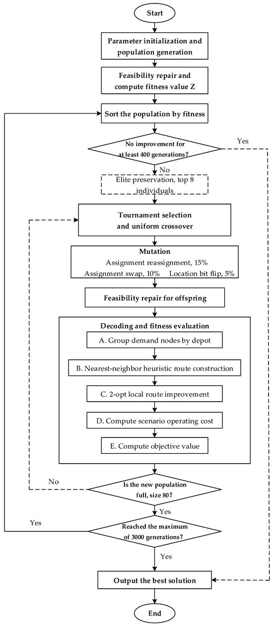
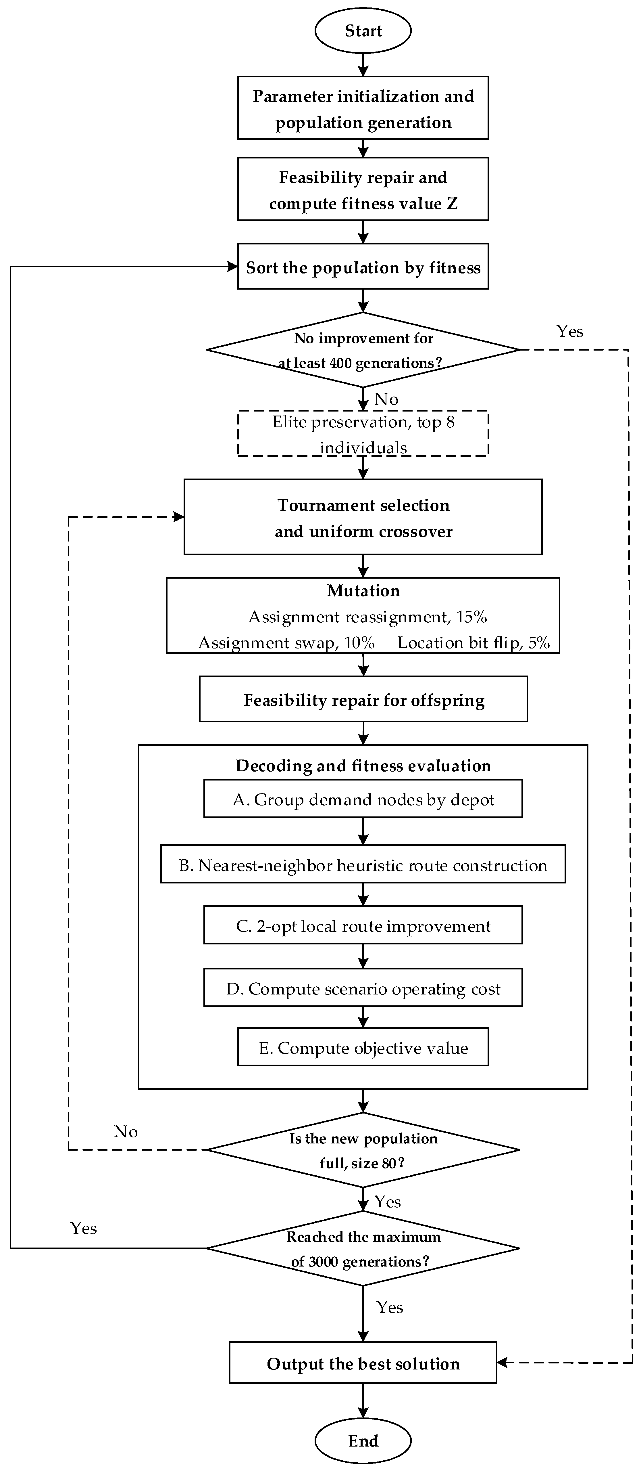
The overall procedure of the improved genetic algorithm is shown in Figure 1. The main steps are as follows.

Figure 1. Improved genetic algorithm flowchart.

Step 1—Initialization. Set algorithm parameters and generate the initial population. Apply feasibility repair and compute fitness for each individual.

Step 2—Elite preservation. Directly retain several individuals with the best fitness in the current generation for the next generation.

Step 3—Selection, crossover, mutation, and evaluation. Use the selection operator to form the mating pool. Apply crossover and mutation to generate offspring. Apply feasibility repair and decoding-based evaluation to offspring and form the next generation.

Step 4—Early stopping check. If the early stopping criterion is met, terminate the iteration. Otherwise, return to Step 2.

Step 5—Output. Output the construction plan of the best individual, the vehicle routes and number of vehicles under each scenario, and each component of the objective function along with the composite objective value.

3. Results

3.1. Test Instance Analysis

3.1.1. Test Instance Description and Parameter Settings

We evaluate the proposed improved genetic algorithm on six benchmark instances from the Prodhon dataset. The goal is to test its effectiveness for the shared e-bike battery-swapping station location–routing problem. The instances are 20-5-1, 20-5-2, 50-5-1, 50-5-2, 100-5-1, and 100-5-2. These instances cover three typical scales, including small, medium, and relatively large problem settings.

The original Prodhon instances focus on the location-routing problem and do not include explicit time-window constraints. Battery-swapping operations for shared electric bikes exhibit clear time-sensitivity. To better reflect practical operating conditions, we generate a service time window for each demand node while keeping the spatial distribution, demand scale, and construction cost unchanged. The time-window width for each customer node is randomly sampled from 40 min to 200 min. The service time is fixed at 5 min to represent the processing time of battery swapping. The vehicle travel speed is set to 25 km/h. This speed is used to convert travel distance into travel time and to trigger time-window penalties. Apart from the time-window and speed settings, all other model and cost parameters follow the original benchmark values. These settings retain the Prodhon data structure and introduce time-related constraints with clear transportation meaning. They allow the model to be evaluated in terms of both timeliness and route organization.

All experiments were conducted on a workstation equipped with an Intel Core i5-12400 processor (Intel, Santa Clara, CA, USA), 32 GB RAM, running Windows 10, with implementations developed in Python 3.12. Weather uncertainty is represented by two scenarios, no rain (NR) and rain (R). Scenario probabilities are obtained from frequency statistics of weather records over 31 consecutive days in the study area, yielding ${\rho }_{NR}=23/31$ and ${\rho }_R=8/31$. Weather impacts travel time and transportation cost through a scenario-dependent road impedance multiplier ${\gamma }_{ijs}$. As a baseline setting, we use ${\gamma }_{ijNR}=1.0$ and ${\gamma }_{ijR}=1.25$, which represent a 25% increase in effective travel impedance under rain. The risk penalty coefficient $\kappa$ is set to 0.3. It controls the weight of the worst-case operating cost upper bound in the objective function. This setting balances expected cost and risk control.

The improved genetic algorithm is developed in this study. After repeated runs and parameter tuning, the final parameter settings are obtained. The parameter settings are summarized in Table 4.

Table 4. Improved genetic algorithm parameter settings.

Parameters	Meaning	Value
pop_size	Population size	80
generations	Maximum iteration count	3000
elite_size	Elite retention size	8
early_stop_patience	Early stopping patience generations	400
init_build_num	Initial number of individuals range	2~4
tournament_k	Tournament selection size	3
crossover_rate_w	Site vector crossover probability	0.5
crossover_rate_assign	Allocation vector crossover probability	0.5
mutate_flip_w	Site switch mutation probability	0.05
mutate_reassign_prob	Redistribution mutation probability	0.15
mutate_swap_prob	Allocation swap mutation probability	0.1

3.1.2. Analysis of Results

Table 5 shows that IGA achieves better objective values across all six test instances. Compared with LNS, IGA improves the objective value by about 0.27%, 0.09%, 3.18%, 1.19%, 0.04%, and 0.62% for the six instances. The improvements are more pronounced for small and medium instances, while the gains are smaller for large instances. This indicates that, as problem size increases, both methods can approach good solutions, but IGA maintains a stable advantage. Compared with the standard GA, IGA improves the objective value by about 0.76%, 0.70%, 6.75%, 4.79%, 2.43%, and 2.58% for the six instances. The improvement persists across all scales. This suggests that the standard GA is more likely to stagnate at relatively poor solutions in coupled location and routing optimization, whereas IGA yields higher-quality integrated plans.

Table 5. Algorithm performance comparison results.

Instance	IGA		LNS		GA
	Objective Function	Execution Time	Objective Function	Execution Time	Objective Function	Execution Time
20-5-1	28,323.68	2.1 s	28,399.96	9.2 s	28,540.07	6.5 s
20-5-2	29,575.59	1.4 s	29,602.36	13.7 s	29,784.10	8.6 s
50-5-1	31,548.04	26.3 s	32,582.24	57.8 s	33,832.69	46.7 s
50-5-2	46,383.91	7.8 s	46,942.46	125.8 s	48,715.13	40.1 s
100-5-1	166,631.68	139.2 s	166,703.23	214.1 s	170,775.28	72.8 s
100-5-2	129,633.16	183.6 s	130,442.96	266.3 s	133,065.99	119.0 s

In terms of computational efficiency, IGA requires less runtime than LNS for all six instances, with reductions of about 77.2%, 89.8%, 54.5%, 93.8%, 35.0%, and 31.1%. This indicates that, as instance size increases, the computational cost of the destroy-and-repair operations in LNS grows more rapidly. Compared with the standard GA, IGA runs faster in four instances, with reductions of about 67.7%, 83.7%, 43.7%, and 80.5%. This shows that IGA achieves both solution quality and efficiency advantages for small and medium problems. It should be noted that, for the two 100-node instances, the runtime of IGA increases by about 91.2% and 54.3%, respectively, while still producing better objective values. This implies that, for larger problems, the improved GA trades higher computational effort for better solution quality through more extensive search and evaluation. It reflects a trade-off between accuracy and efficiency.

Overall, IGA attains better objective values on all six instances and shows a clear computational efficiency advantage over LNS. Relative to the standard GA, it achieves simultaneous improvements in both quality and runtime for small and medium instances, while for large instances it produces higher-quality solutions at a higher computational cost. These results demonstrate that IGA is effective and applicable to the battery-swapping station location-routing optimization model developed in this study, which incorporates weather scenarios and a risk penalty.

3.2. Case Study

3.2.1. Case Description

The case data in this study primarily originate from mobile applications of shared electric bicycle platforms and map coordinate collection. Within the platform application’s docking station page, users may query vehicle information at that location, with the battery charge status of individual bicycles displayed. Low battery levels are indicated by a prominent marker, and when users attempt to scan the QR code to use a bicycle, a prompt is provided indicating whether unlocking is possible. Based on this information presentation mechanism, this study defines vehicles displaying insufficient battery and an unlock failure prompt as the basis for determining battery swap demand. When a vehicle shows low battery and an unlock failure message, it indicates the vehicle has exited serviceable status, creating an immediate battery swap requirement. Accordingly, the number of vehicles in this state at a docking point during the observation period is defined as the battery swap demand for that point, which is further utilized to construct demand point parameters.

To reduce random fluctuations from a single observation and to improve the stability and representativeness of demand characterization, we adopt a monitoring scheme of one observation per day over one consecutive month and use the average as the representative value. The monitoring period is from 1 August 2025 to 31 August 2025. Observations are conducted at fixed locations during 7:00–9:00 each day. The observation times are kept as consistent as possible to improve comparability. During the monitoring period, the observed demand values at each parking point are aggregated. The monthly average is then computed to obtain a representative demand intensity for each parking point, which serves as an input parameter of the model.

For spatial data construction, parking-point locations are verified using platform information. Latitude and longitude coordinates of parking points are extracted using a map coordinate acquisition tool. This yields the demand-node set for the case study. Compared with the synthetic instances, the real-world case study does not use Euclidean distance to measure inter-node travel. Road-network shortest-path distances $d_{ij}$ are obtained by batched route-planning queries between any two nodes using the Baidu Map Direction API under driving mode.

For service constraints, after a battery-swapping vehicle arrives at a parking point, it must complete tasks such as locating the vehicle, replacing the battery, and confirming the status. The service time increases with the number of batteries swapped. To capture differences in workload, the service time at each point is set as the sum of a fixed basic operation time and an incremental time that depends on the battery-swapping quantity. The basic operation time after arrival is set to 5 min. An additional 10 s is added for each battery. This defines the service-time parameter for each parking point. Detailed information on parking points and candidate battery-swapping station sites is provided in Table 6 and Table 7. Only partial data are shown here, and the omitted rows are represented by ellipses.

Table 6. Information of case parking point.

Number	Longitude	Latitude	Demand	Time Window	Service Hours
D1	114.511237	38.095628	20	07:22	8.33 min
D2	114.512386	38.094340	15	07:31	7.50 min
D3	114.509481	38.091693	9	07:22	6.50 min
…	…	…	…	…	…
D60	114.518511	38.065423	9	07:50	6.50 min
D61	114.518443	38.068869	9	07:17	6.50 min
D62	114.518650	38.071540	16	07:55	7.67 min

Table 7. Information on alternative battery swap stations.

Number	Longitude	Latitude	Station Capacity	Annual Rent
C1	114.514000	38.068755	250	96,000 CNY
C2	114.514901	38.080115	250	105,000 CNY
C3	114.521039	38.069501	250	112,000 CNY
C4	114.524730	38.077118	250	99,000 CNY
C5	114.527392	38.066222	250	101,000 CNY

3.2.2. Parameter Settings

Regarding parameter settings, all cost and operational parameters are taken from the operator’s real operational data. The unit distance transport cost is set at 5 CNY per kilometer. The unit time penalty cost is set at 1 CNY per minute. The fixed vehicle deployment cost is set at 200 CNY. The battery capacity of delivery vehicles is set at 85 units. The average vehicle speed is set at 25 km/h. The algorithm parameters are identical to those used in the Test Instance Analysis.

3.2.3. Analysis of Results

(1)

Algorithm Convergence Characteristics:

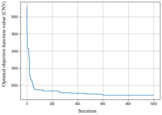
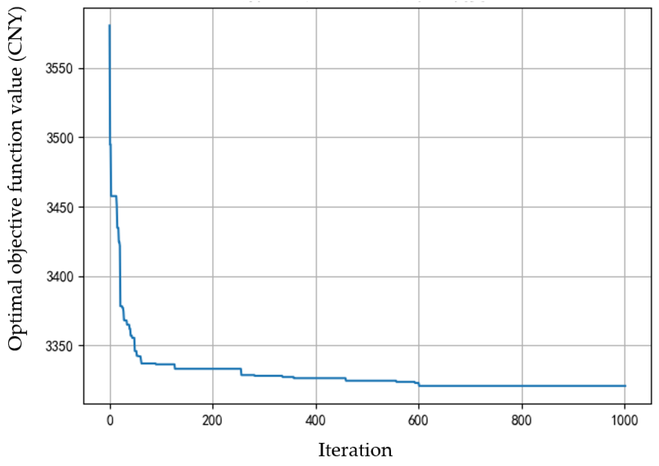
To validate the effectiveness and stability of the designed algorithm in solving location and routing problems that incorporate weather scenarios and risk penalties, this paper presents the convergence curve of the objective function’s optimal value under the genetic algorithm for this case study, as shown in Figure 2.

Figure 2. Improved genetic algorithm convergence curve.

Observing the numerical changes at key iteration points, the algorithm’s optimal objective value had decreased to 3332.94 CNY by the 200th iteration, further reduced to 3326.18 CNY by the 400th iteration, and reached 3322.76 CNY by the 600th iteration. This indicates that improvements to the objective value were more pronounced during the early iterations. By the 800th iteration, the optimal objective value reached 3320.62 CNY and remained unchanged by the 1000th iteration. This indicates that the algorithm approached a stable, near-optimal level in the mid-to-late stages, with marginal gains from further iterations diminishing markedly. This conclusion is further corroborated by the early termination mechanism’s activation. Following 400 consecutive iterations without improvement, the algorithm terminated at iteration 1002, ultimately achieving the objective function’s minimum value of 3320.62 CNY. This process demonstrates that the plateau phase of the convergence curve exhibits distinct stability characteristics. The algorithm showed no significant regression fluctuations or periodic rebounds, reflecting robust convergence reliability. The optimal solution converged by the algorithm was subsequently utilized for site allocation, route organization, and cost comparative analysis.

(2)

Analysis of Delivery Routes Under Two Weather Scenarios:

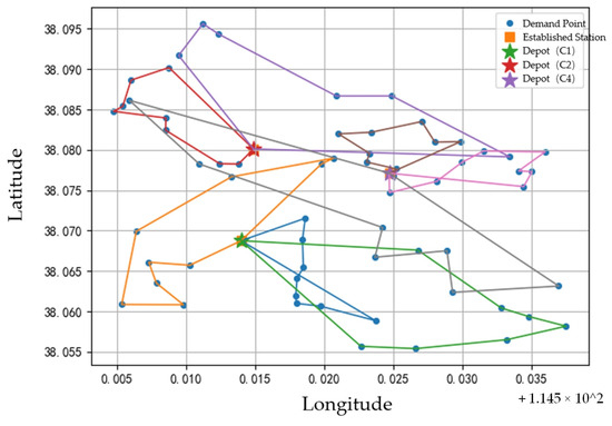
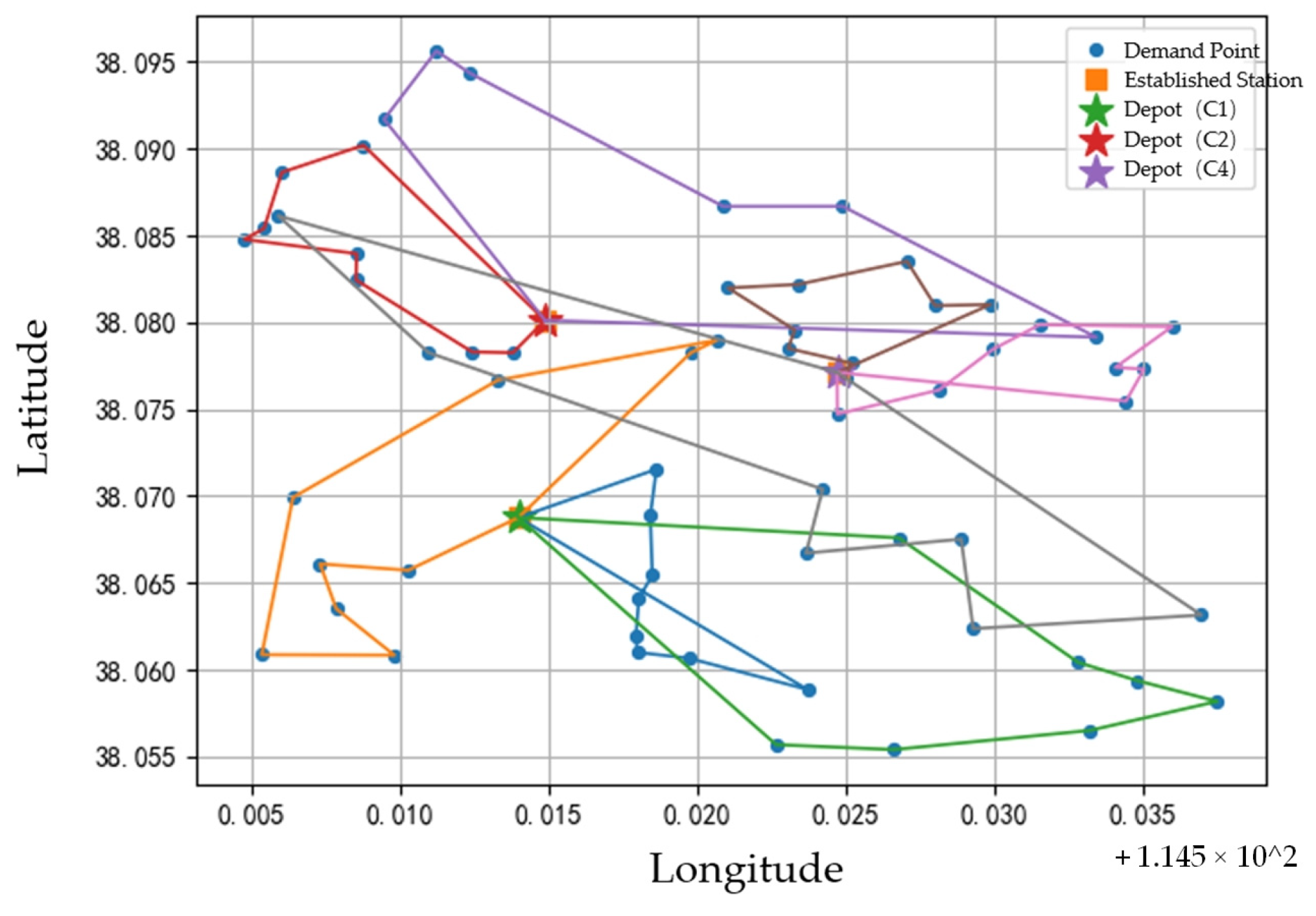
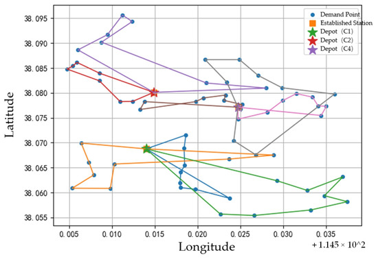
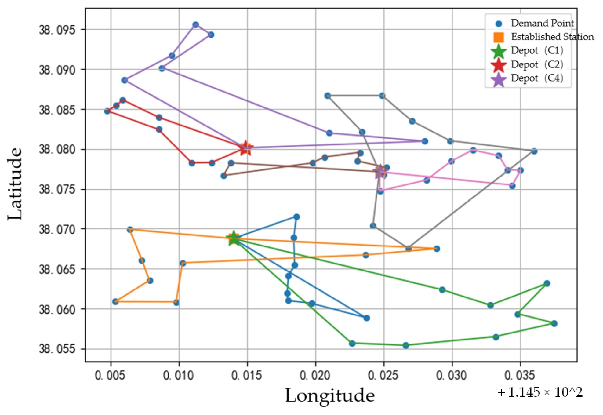
To compare distribution operations under the no rain and rain scenarios, we present route maps and detailed routing tables for both scenarios. The route map for the no rain scenario is shown in Figure 3, and the route map for the rain scenario is shown in Figure 4. The route map is used only to present the service sequence and assignment results. In model solving, $d_{ij}$ denotes the road-network shortest-path distance obtained from the Direction API, rather than the straight-line distance shown in the figure.

Figure 3. Schematic of vehicle delivery routes under the NR scenario.

Figure 4. Schematic of vehicle delivery routes under the R scenario.

The number of activated vehicles is 8 in both scenarios. This indicates that fleet size is mainly determined by total demand and vehicle capacity, and that weather has a limited impact on the required number of vehicles. In the no rain scenario, the transportation distance cost is 192.40 CNY, and the lateness penalty cost is 92.49 CNY. The scenario operating cost is 1884.89 CNY. In the rain scenario, the transportation distance cost is 217.74 CNY, and the lateness penalty cost is 133.32 CNY. The scenario operating cost is 1951.06 CNY. Both the transportation distance cost and the lateness penalty cost increase, leading to an increase of 66.17 CNY in scenario operating cost.

This indicates that the amplified impedance under rain primarily affects operational efficiency through increased arrival delays caused by reduced travel efficiency and through higher effective transportation costs. Some vehicles maintain identical or similar service chains across the two scenarios, which suggests that the spatial clustering structure of demand nodes imposes stable constraints on route patterns. At the same time, several vehicles exhibit reorganization of visiting sequences and service areas. Under rain conditions, the routing tends to reduce the cumulative impact of high-impedance links by adjusting the chaining of demand nodes and the cross-area connections, thereby mitigating delay risk. This result indicates that the model can capture the time pressure under rain during scenario evaluation and adapt to adverse weather through route-structure adjustments. The fleet size remains unchanged across scenarios while route structures are reorganized. This implies that the model absorbs weather-induced impedance changes mainly through routing decisions rather than by deploying additional vehicles to hedge risk.

The detailed vehicle routing plans under the two weather scenarios are summarized in Table 8 and Table 9. The service quantity in the tables is the number of batteries delivered by each vehicle. The utilization rate is computed using a vehicle capacity of 85 batteries. The comparison shows that vehicle loads are generally high. Most primary trips exceed 90% utilization, which indicates effective use of vehicle capacity. Meanwhile, under the rain scenario, delays increase substantially on multiple routes and become more dispersed. This reflects the uneven impact of weather disturbances on time-related constraints. Some service chains are more sensitive to impedance amplification.

Table 8. Vehicle routing plan details under the NR scenario.

Delivery Vehicle	Station	Delivery Route	Service Quantity	Utilization Rate	Delay Time
V1	C1	C1⟶D62⟶D61⟶D60⟶D59⟶D58⟶D57⟶D26⟶D34⟶C1	81	95.3%	3.3 min
V2	C1	C1⟶D38⟶D36⟶D14⟶D51⟶D52⟶D56⟶D53⟶D54⟶D55⟶C1	85	100.0%	21.2 min
V3	C1	C1⟶D33⟶D45⟶D18⟶D32⟶D44⟶D31⟶D30⟶C1	62	72.9%	1.9 min
V4	C2	C2⟶D4⟶D5⟶D7⟶D8⟶D9⟶D10⟶D12⟶D13⟶C2	85	100.0%	2.7 min
V5	C2	C2⟶D3⟶D1⟶D2⟶D15⟶D37⟶D25⟶C2	79	92.9%	12.8 min
V6	C4	C4⟶D50⟶D49⟶D48⟶D47⟶D23⟶D16⟶D29⟶D17⟶D43⟶C4	82	96.5%	33.1 min
V7	C4	C4⟶D35⟶D21⟶D24⟶D46⟶D39⟶D22⟶D41⟶D19⟶C4	78	91.8%	13.5 min
V8	C4	C4⟶D6⟶D11⟶D42⟶D40⟶D28⟶D27⟶D20⟶C4	83	97.6%	4.0 min

Table 9. Vehicle routing plan details under the R scenario.

Delivery Vehicle	Station	Delivery Route	Service Quantity	Utilization Rate	Delay Time
V1	C1	C1⟶D62⟶D61⟶D60⟶D59⟶D58⟶D57⟶D26⟶D34⟶C1	81	95.3%	5.6 min
V2	C1	C1⟶D28⟶D40⟶D55⟶D56⟶D52⟶D53⟶D54⟶D51⟶C1	80	94.1%	17.0 min
V3	C1	C1⟶D33⟶D45⟶D18⟶D32⟶D44⟶D20⟶D31⟶D27⟶C1	80	94.1%	11.4 min
V4	C2	C2⟶D9⟶D6⟶D7⟶D8⟶D10⟶D11⟶D12⟶C2	80	94.1%	6.5 min
V5	C2	C2⟶D5⟶D3⟶D1⟶D2⟶D4⟶D23⟶D17⟶C2	78	91.8%	33.8 min
V6	C4	C4⟶D50⟶D49⟶D48⟶D47⟶D36⟶D38⟶D14⟶D13⟶C4	79	92.9%	13.3 min
V7	C4	C4⟶D35⟶D21⟶D24⟶D46⟶D25⟶D22⟶D41⟶D19⟶C4	82	96.5%	15.3 min
V8	C4	C4⟶D16⟶D15⟶D37⟶D29⟶D43⟶D39⟶D30⟶D42⟶C4	75	88.2%	30.5 min

(3)

Cost Comparison Analysis of Two Scenarios:

To quantify the operational differences between the no rain and rain scenarios and to explain the risk-control role of the robust term under adverse weather, the key cost indicators and objective components of the two scenarios are summarized in Table 10.

Table 10. Cost comparison analysis of the two scenarios.

Indicator	NR Scenarios	R Scenarios	Expected Value
Number of vehicles	8	8	8
Total delay time (min)	92.49	133.32	112.91
Transportation distance cost	192.40	217.74	198.94
Fixed vehicle cost	1600.00	1600.00	1600.00
Lateness penalty cost	92.49	133.32	103.02
Scenario operating cost	1884.89	1951.06	1918.00
Station construction cost	833.33	833.33	833.33
Robust penalty term	585.32	585.32	585.32
Objective value	3320.62	3320.62	3320.62

Table 10 shows that the scenario operating cost is 1884.89 CNY under no rain and 1951.06 CNY under rain. The rain scenario increases the operating cost by 66.17 CNY. The number of vehicles is identical in the two scenarios, and the fixed vehicle cost remains unchanged. This indicates that weather does not lead to changes in fleet size. The cost gap mainly comes from higher transportation distance cost and higher lateness penalty cost. The transportation distance cost increases from 192.40 CNY to 217.74 CNY, an increase of 25.34 CNY. The lateness penalty cost increases from 92.49 CNY to 133.32 CNY, an increase of 40.83 CNY. This indicates that the increase in time pressure under rain is more pronounced and is the main driver of the operating cost increase.

(4)

System Resilience Analysis:

To examine the contribution of the robust penalty term in the risk-averse objective to solution resilience, we compare the performance of a risk-neutral model with $\kappa =0$ and a risk-averse model with $\kappa =0.3$ under the same case data and parameter settings. The two models yield the same battery-swapping station location plan and the same number of activated vehicles. Therefore, the station construction cost and fixed vehicle activation cost remain unchanged. The differences are mainly reflected in the transportation distance cost and the soft time-window lateness penalty at the operational level. The results are reported in Table 11. This comparison isolates the effect of the robust penalty term on mitigating operating losses under the adverse weather scenario and avoids interference from fixed investment terms.

Table 11. System resilience analysis under different robust penalty coefficients.

Scenario	Robust Penalty Coefficient	Transportation Distance Cost	Lateness Penalty Cost	Variable Operating Cost
NR	$\kappa$ = 0	180.38	91.96	272.34
	$\kappa$ = 0.3	192.40	92.49	284.89
R	$\kappa$ = 0	234.10	136.73	370.83
	$\kappa$ = 0.3	217.74	133.32	351.06

Under the NR scenario, the variable operating loss is 272.34 CNY when $\kappa =0$ and 284.89 CNY when $\kappa =0.3$, an increase of 12.55 CNY. This difference is mainly due to an increase of 12.02 CNY in transportation distance cost and an increase of 5.33% in lateness penalty cost. The cost breakdown across the two scenarios suggests that the impact of weather disturbances on operating loss is primarily driven by reduced traffic efficiency, which delays arrivals and increases lateness risk. It is not determined only by geometric mileage changes. This implies that, under normal weather, the solution tends to adopt more conservative routing and service sequences to maintain stable performance under adverse conditions, which leads to modest efficiency loss.

Under the rain scenario R, the variable operating loss is 370.83 CNY when $\kappa =0$ and 351.06 CNY when $\kappa =0.3$, a decrease of 19.77 CNY. This indicates that the robust model can effectively suppress operating loss under adverse weather. In terms of components, the transportation distance cost decreases by 16.36 CNY and the lateness penalty cost decreases by 3.41 CNY. The corresponding total delay time decreases by 3.41 min. The resilience gain can be quantified as a reduction of about 5.33% in variable operating loss under the rain scenario. Moreover, the shock in variable operating loss when moving from no rain to rain is 98.49 CNY for $\kappa =0$, and it decreases to 66.17 CNY for $\kappa =0.3$. The shock reduction is about 32.82%. These results show that introducing the robust penalty term substantially enhances the solution’s resistance to adverse-weather disturbances. It enables more stable time and cost performance under unfavorable conditions and improves system resilience.

3.3. Sensitivity Analysis

3.3.1. Impact of the Road Impedance Multiplier on Results

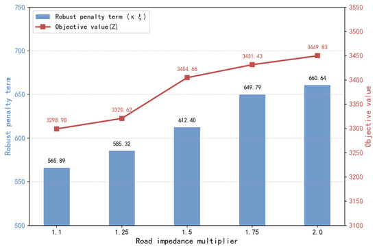
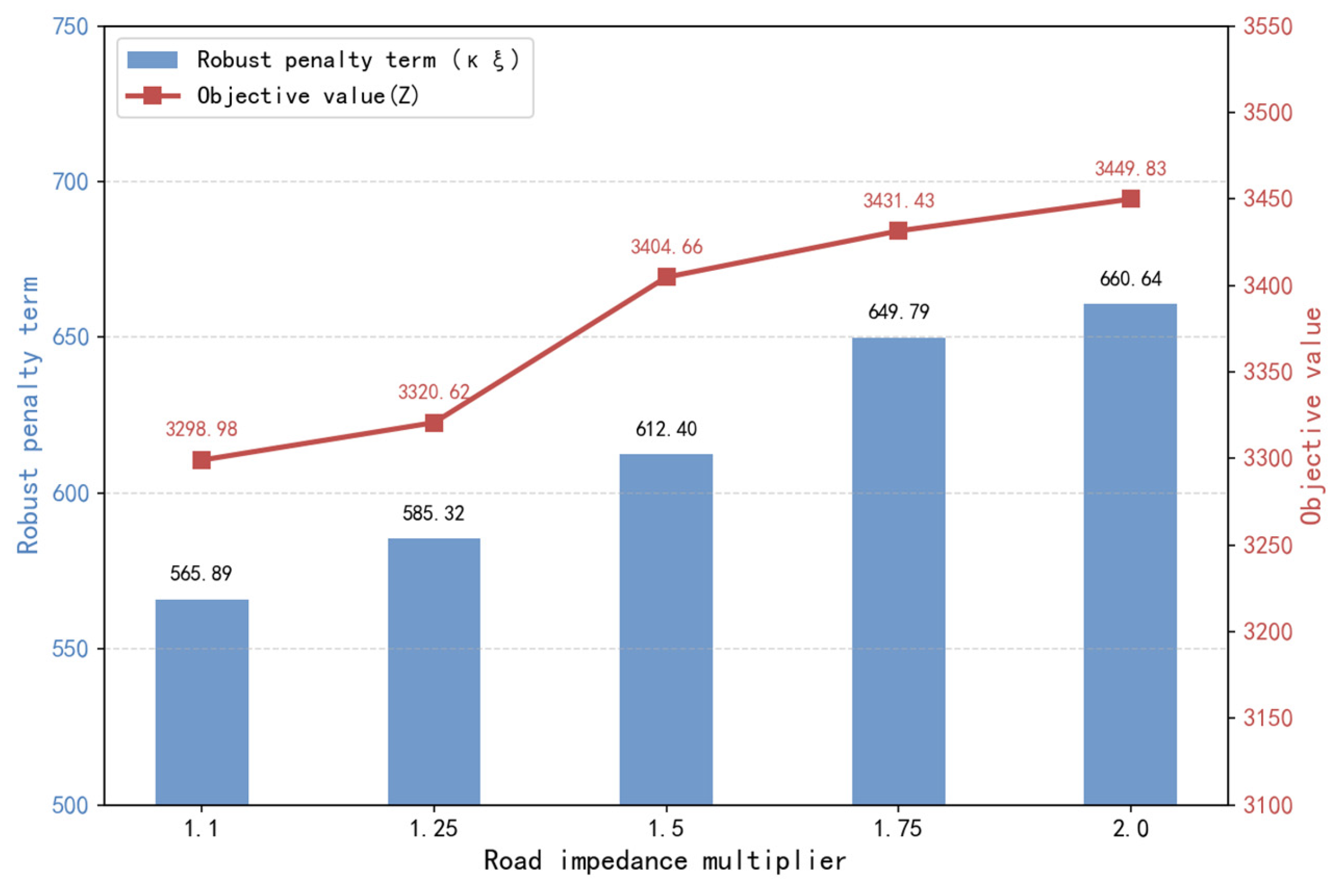
To examine how the reduction in travel efficiency under rain affects decision outcomes, we conducted a one-factor sensitivity analysis while keeping all baseline parameters unchanged. The value of ${\gamma }_{ijs}$ is set to 1.10, 1.25, 1.50, 1.75, and 2.00. The results are shown in Figure 5.

Figure 5. Sensitivity analysis results for the road impedance multiplier.

According to Equation (3), ${\gamma }_{ijs}$ scales transportation cost through impedance amplification. It also changes travel time and therefore affects the lateness penalty term. As a result, it simultaneously changes the transportation cost and the lateness penalty under the rain scenario. It further increases the worst-case upper bound.

Figure 5 shows a clear increase in total system cost as ${\gamma }_{ijs}$ increases. The total cost rises from 3298.98 CNY to 3449.83 CNY and follows a stable monotonic trend. The robust penalty term increases from 565.89 CNY to 660.64 CNY, with a substantial rise. This indicates that higher rain impedance not only increases the expected operating cost under the rain scenario, but also pushes up the worst-case cost upper bound, which in turn increases the robust penalty term.

3.3.2. Impact of the Robust Penalty Coefficient on Results

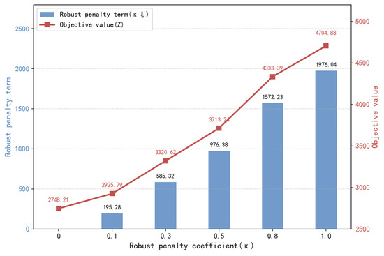
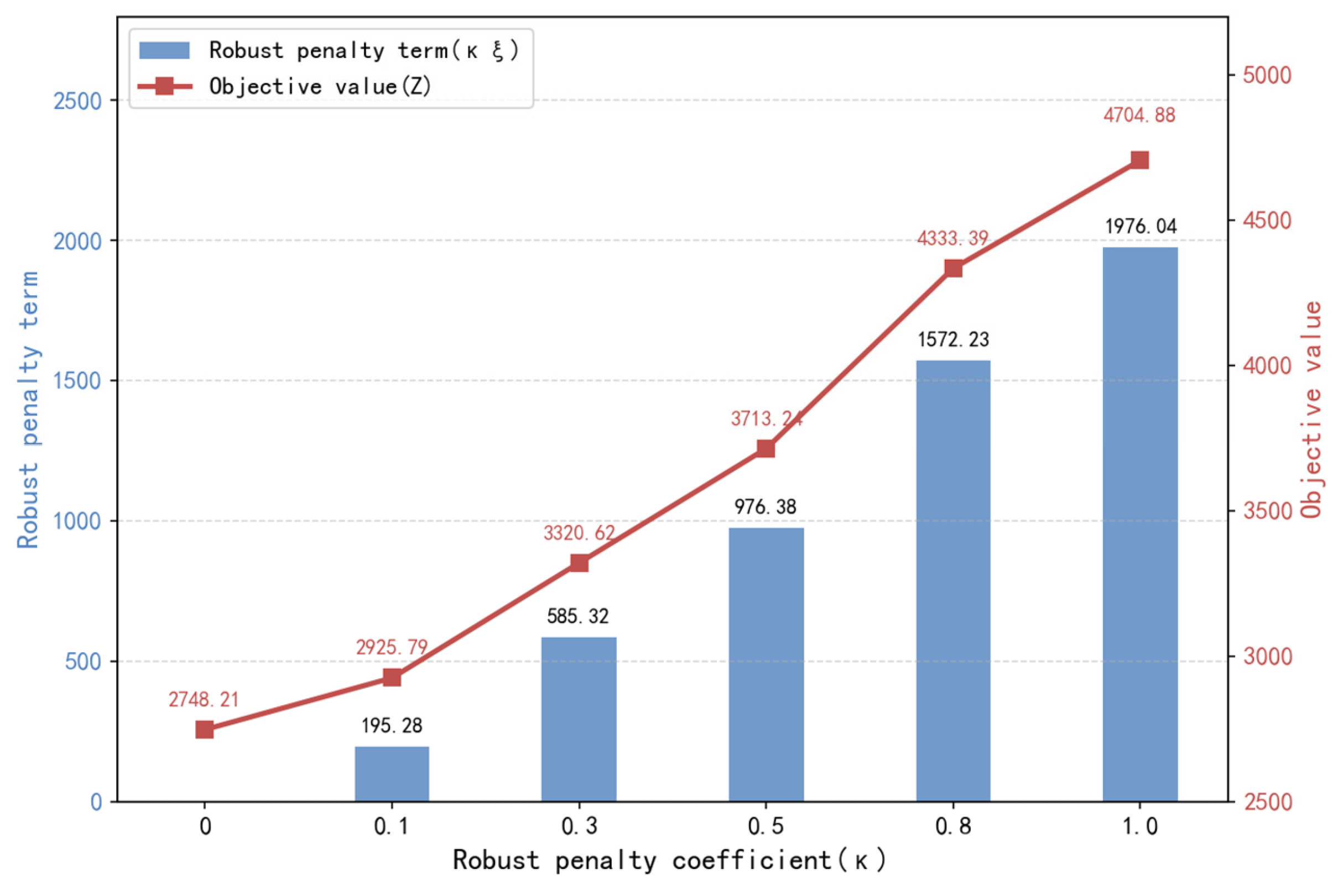
To characterize the trade-off between expected cost and worst-case risk under different risk preferences, we conduct a sensitivity analysis by varying $\kappa$ while keeping all baseline parameters unchanged. The value of $\kappa$ is set to 0, 0.1, 0.3, 0.5, 0.8, and 1.0. The results are shown in Figure 6.

Figure 6. Sensitivity analysis results for the robust penalty coefficient.

According to Equation (1), $\kappa$ directly determines the weight of the worst-case penalty term in the objective function. It is a preference-based parameter. A larger $\kappa$ places greater emphasis on worst-case risk and drives the solution toward more stable and conservative decisions.

Figure 6 shows that $\kappa$ has the most pronounced impact on total system cost and that the overall trend is monotonic increasing. When $\kappa$ increases from 0 to 1.0, the total system cost rises from 2748.21 to 4704.88 CNY, with a substantial increase. At the same time, the robust penalty cost increases from 0 to 1976.04 CNY. This pattern is consistent with the objective structure. The robust penalty cost is amplified by $\kappa$, which leads to a marked increase in the total objective value. In contrast, changes in the expected operating cost term are not dominant. This indicates that the primary role of $\kappa$ is to adjust the weight of risk penalization rather than to directly change the expected cost level.

This increase in total system cost should be interpreted carefully. A higher $\kappa$ does not imply a worse plan. It reflects a higher willingness to pay for worst-case stability under greater risk aversion. In practical applications, $\kappa$ can be used as a parametric representation of an operator’s risk preference or desired service assurance level. In this case study, the baseline value $\kappa =0.3$ represents a moderate trade-off between expected cost and worst-case risk and has clear practical interpretability.

4. Discussion

This research employs a scenario-based optimization framework with two weather scenarios. It integrates binary location decisions for battery-swapping station construction with scenario-dependent routing and scheduling decisions specific to each scenario. The formulation balances average efficiency against extreme risk by jointly optimizing expected cost and worst-scenario penalties. At the constraint level, the model embeds key operational mechanisms as hard feasibility boundaries, including depot supply capacity limits, travel impedance adjustments under adverse weather, as well as time windows and subtour elimination; meanwhile, delay penalties are used to represent soft time-window violations, without relaxing the structural feasibility requirement that each parking location must be visited exactly once, thereby ensuring implement ability and a guaranteed service baseline across scenarios. The computational results further reveal that construction decisions remain a dominant driver of system economics, substantially exceeding the scenario-weighted operating costs, indicating that facility layout is a key lever shaping overall cost; concurrently, the worst-scenario operating cost characterizes an upper bound on cost exposure under adverse weather, and an appropriate robustness weight induces a moderate robustness premium, enabling the system to constrain low-probability, high-impact risks and enhance disturbance tolerance without unduly sacrificing day-to-day cost efficiency. Methodologically, an improved genetic algorithm (IGA) is developed, following a two-part encoding and decoding architecture, which avoids directly encoding large-scale arc variables in chromosomes and constructs executable vehicle routes dynamically based on scenario-wise assignments, thereby providing a complexity-based explanation for tractability at moderate scales and potential scalability. In addition, the experimental design and the scenario probability configuration, estimated from frequency statistics over 31 consecutive days in the monitoring period, offer a reproducible modeling pathway for practical deployment. For the real-world case study, inter-node distances are obtained from the Baidu Map Direction API under driving mode to construct road-network shortest-path distances, rather than using Euclidean distance, which improves practical validity. Nevertheless, several limitations merit discussion: scenario probabilities and impact parameters are treated as exogenous with full information available to the decision maker, and the weather impact is represented by an aggregated impedance multiplier rather than time-dependent congestion dynamics, which may be optimistic in real operations; moreover, the case size remains limited, and further validation is needed on larger urban networks and under more complex multi-vehicle settings with explicit labor constraints and dynamic battery inventory evolution. In practice, disruption response is often a continuous process that requires repeated adjustment as information updates, for example, when weather forecasts change or congestion propagates. Future work will extend the proposed framework to a rolling-horizon setting. In this extension, station decisions remain fixed over a planning horizon, while routes and inventory allocation are updated periodically using real-time travel conditions and weather forecasts. The robust penalty mechanism can be retained to hedge against worst-case outcomes within each rolling window. Future research may therefore retain the scenario-based structure while incorporating data-driven scenario updating or distributionally robust formulations to reduce reliance on prior probabilities, and further integrate multi-period rolling-horizon optimization, real-time re-optimization, and finer-grained resource dynamics, so as to improve the explanatory power and transferability of the proposed framework for coordinated governance of normal-state efficiency and abnormal-state stability in real-world SEB battery-swapping systems.

5. Conclusions

This study addresses weather-related operational risk in shared e-bike battery-swapping systems, where rainy conditions may reduce travel efficiency and increase time-window violations, and accordingly develops a joint optimization framework for battery-swapping station siting and swapping logistics routing under uncertainty. The proposed approach follows a two-scenario weather-based formulation that couples station construction decisions with scenario-dependent routing and scheduling within a single model and captures a tunable trade-off between efficiency and resilience through an objective structure combining expected cost and worst-scenario penalties. Meanwhile, structural feasibility and a guaranteed service baseline across scenarios are ensured by a constraint system incorporating depot supply capacity limits, scenario-dependent impedance adjustments, time windows, and subtour elimination.

The computational study demonstrates a pronounced facility-driven cost structure, indicating that station layout is a primary lever governing system economics. The worst-scenario operating cost characterizes an upper bound on cost exposure under adverse weather; by applying a robustness weight, it yields a moderate robustness premium, thereby constraining low-probability, high-impact risks and enhancing disturbance tolerance without unduly sacrificing day-to-day cost efficiency. To address the fact that deterministic formulations may introduce a large number of arc variables and thus incur rapidly escalating computational burden, we develop an improved genetic algorithm with construction encoding and scenario-wise assignment encoding, where feasibility repair is applied before evaluation and routes are generated during decoding with local improvement. The algorithm exhibits stable convergence, maintaining near-optimal objective values in later iterations, and produces implementable station deployment and routing plans under both the no-rain and rain scenarios. The System Resilience Analysis shows that the robust penalty term reduces variable operating loss under rain by 5.33% and cuts the cost shock from no rain to rain by 32.82%. This indicates stronger resistance to adverse-weather disturbances and improved system resilience. Sensitivity analyses further show that increasing the rain impedance multiplier raises both operating cost and the worst-case penalty, while increasing the robustness weight increases total objective value by amplifying the worst-case term, reflecting a clear trade-off between expected cost and robustness.

References

- Lu, X.; Cheng, C. Locating facilities with resiliency to capacity failures and correlated demand uncertainty. Transp. Res. Part E Logist. Transp. Rev. 2021, 153, 102444. [Google Scholar] [CrossRef] [Scilit]
- Cheng, C.; Adulyasak, Y.; Rousseau, L.-M. Robust facility location under demand uncertainty and facility disruptions. Omega 2021, 103, 102429. [Google Scholar] [CrossRef] [Scilit]
- Cheng, C.; Yu, Q.; Adulyasak, Y.; Rousseau, L.-M. Distributionally robust facility location with uncertain facility capacity and customer demand. Omega 2024, 122, 102959. [Google Scholar] [CrossRef] [Scilit]
- Chen, Y.; Li, D.; Zhang, Z.; Wahab, M.I.M.; Jiang, Y. Solving the battery swap station location-routing problem with a mixed fleet of electric and conventional vehicles using a heuristic branch-and-price algorithm with an adaptive selection scheme. Expert Syst. Appl. 2021, 186, 115683. [Google Scholar] [CrossRef] [Scilit]
- Li, Y.; Li, F.; Li, Q.; Zhang, P. Battery swapping station location routing problem: A cooperative business model. Comput. Ind. Eng. 2025, 200, 110775. [Google Scholar] [CrossRef] [Scilit]
- Cao, Z.; Mao, Z.; Wang, Y.; Zhang, S. Multi-Type Electric Vehicle Scheduling Optimization Considering Load Capacity, Battery-Allowed Mileage, and Recharging Duration. Electronics 2023, 12, 4655. [Google Scholar] [CrossRef] [Scilit]
- Chen, G.; Gao, J.; Chen, D. Research on Vehicle Routing Problem with Time Windows Based on Improved Genetic Algorithm and Ant Colony Algorithm. Electronics 2025, 14, 647. [Google Scholar] [CrossRef] [Scilit]
- Cai, Z.; Shen, R.; Yu, C.; Xiang, X. Joint Routing Optimization of Autonomous Vehicles Under Recharging and Battery-Swapping Modes. Electronics 2025, 14, 4880. [Google Scholar] [CrossRef] [Scilit]
- Cai, H.; Xu, P.; Tang, X.; Lin, G. Solving the Vehicle Routing Problem with Stochastic Travel Cost Using Deep Reinforcement Learning. Electronics 2024, 13, 3242. [Google Scholar] [CrossRef] [Scilit]
- Shao, S.; Li, D.; Zhou, Y.; Sheu, J.-B. Optimizing battery swapping for city-scale e-bike sharing systems: A three-stage spatial–temporal cluster-based approach. Transp. Res. Part E Logist. Transp. Rev. 2025, 198, 104145. [Google Scholar] [CrossRef] [Scilit]
- Zhou, Y.; Lin, Z.; Guan, R.; Sheu, J.-B. Dynamic battery swapping and rebalancing strategies for e-bike sharing systems. Transp. Res. Part B Methodol. 2023, 177, 102820. [Google Scholar] [CrossRef] [Scilit]
- Xu, M.; Di, Y.; Zhu, Z.; Yang, H.; Chen, X. Designing van-based mobile battery swapping and rebalancing services for dockless e bike-sharing systems based on the dueling double deep Q-network. Transp. Res. Part C 2022, 138, 103620. [Google Scholar] [CrossRef] [Scilit]
- Jin, Z.; Ma, D.; Li, P.; Li, Y.; Zhang, L. Managing shared electric micromobility systems: Allocation planning and battery swapping. Transp. Res. Part E 2025, 198, 104108. [Google Scholar] [CrossRef] [Scilit]
- Lee, G.; Lee, J.S.; Park, K.S. Battery swapping, vehicle rebalancing, and staff routing for electric scooter sharing systems. Transp. Res. Part E 2024, 186, 103540. [Google Scholar] [CrossRef] [Scilit]
- Jin, X.; Dong, H.; Cao, Y.; Yang, Y. Rebalancing an e-scooter-sharing system with en-route charging capability. Transp. Res. Part C 2025, 180, 105295. [Google Scholar] [CrossRef] [Scilit]
- Ma, H.; Yang, T. Improved Adaptive Large Neighborhood Search Combined with Simulated Annealing (IALNS-SA) Algorithm for Vehicle Routing Problem with Simultaneous Delivery and Pickup and Time Windows. Electronics 2025, 14, 2375. [Google Scholar] [CrossRef] [Scilit]
- Jin, Z.; Li, P.; Li, Y.; Ma, D.; Ren, X.; Wu, L. Target-oriented distributionally robust optimization for battery swapping in shared micromobility systems. Omega 2025, 138, 103436. [Google Scholar] [CrossRef] [Scilit]
- Yu, C.; Liu, L. Robust battery swapping for e-bike sharing with uncertain covariates and partial outsourcing. Omega 2025, 138, 103385. [Google Scholar] [CrossRef] [Scilit]
- Guo, Y.; Yan, K.; Qian, X.; Li, X.; Hu, Y.; Wang, N. A robust optimal battery swapping station location model for commercial electric vehicles under demand uncertainty. Energy 2025, 333, 137466. [Google Scholar] [CrossRef] [Scilit]
- Zhang, F.; Lyu, H.; Ji, Y.; Wong, M.; Kuai, C.; Fan, J. Battery swapping demand simulation for electric micromobility vehicles considering multi-source information interaction and behavior decision. J. Clean. Prod. 2023, 414, 137525. [Google Scholar] [CrossRef] [Scilit]
- Lv, H.; Zhang, F.; Wong, M.; Xing, Q.; Ji, Y. Activity-based travel chain simulation for battery-swapping demand of electric micromobility vehicles. Transp. Res. Part D Transp. Environ. 2024, 126, 104022. [Google Scholar] [CrossRef] [Scilit]
- Zhang, F.; Lv, H.; Xing, Q.; Ji, Y. Deployment of battery-swapping stations: Integrating travel chain simulation and multi-objective optimization for delivery electric micromobility vehicles. Energy 2024, 290, 130252. [Google Scholar] [CrossRef] [Scilit]
- Schulz, A.; Boysen, N.; Briskorn, D. Centrally-chosen versus user-selected swaps: How the selection of swapping stations impacts standby battery inventories. Eur. J. Oper. Res. 2024, 319, 726–738. [Google Scholar] [CrossRef] [Scilit]
Disclaimer/Publisher’s Note: The statements, opinions and data contained in all publications are solely those of the individual author(s) and contributor(s) and not of MDPI and/or the editor(s). MDPI and/or the editor(s) disclaim responsibility for any injury to people or property resulting from any ideas, methods, instructions or products referred to in the content. |
© 2026 by the authors. Licensee MDPI, Basel, Switzerland. This article is an open access article distributed under the terms and conditions of the Creative Commons Attribution (CC BY) license.