APF-Driven Lightweight UAV Swarm Trajectory Optimization in GNSS-Denied Air–Terrestrial Navigation

Abstract

To enable autonomous route planning for UAV swarms in dynamic air–terrestrial cooperative navigation scenarios within GNSS-denied environments, this paper proposes a lightweight framework based on the Artificial Potential Field (APF) method. In the considered architecture, UAVs act as mobile transit navigation nodes that relay positioning information from sparse ground anchors to terrestrial users. For TOA-based cooperative positioning, the instantaneous geometric configuration of the UAV swarm significantly affects the overall system accuracy. Therefore, the impact of UAV positions on the end-to-end navigation performance is rigorously analyzed, yielding a comprehensive Dilution of Precision (DOP) matrix for the entire air–terrestrial system. By applying the Schur complement, the global performance metric is decomposed, resulting in a scalar evaluation function that directly reflects the geometric quality of the configuration. In practical scenarios involving dynamic and heterogeneous users, real-time trajectory adaptation of the UAV swarm is essential to continuously optimize user positioning accuracy. To this end, an APF-based autonomous joint route planning approach is developed. The potential field is constructed directly from the derived geometric evaluation model, where its negative gradient generates virtual forces that autonomously guide the UAV swarm. This elegantly bridges high-level navigation performance optimization with low-level motion control of the swarm. The simulation results show a 76.1% improvement in the average comprehensive GDOP for users compared to the baseline of hovering UAVs, validating the effectiveness and real-time capability of the proposed lightweight framework.

1. Introduction

The rapid advancement of near-ground and low-altitude applications has profoundly impacted economic and military developments. However, in many operational scenarios, the absence of precise position and timing information undermines mission-critical support. Navigation, positioning, and timing (PNT) services have thus become indispensable infrastructure for modern tasks.

Existing navigation solutions for near-ground and low-altitude environments face various limitations, lacking a universally effective approach. Global Navigation Satellite Systems (GNSSs) provide worldwide coverage but are susceptible to interference, jamming, and signal blockage [1]. Inertial navigation systems (INSs) are resilient to external disruptions but suffer from error accumulation over time [2], requiring auxiliary absolute measurements for correction. Matching-based methods, such as visual navigation, rely on prior fingerprint databases and are sensitive to environmental inaccuracies or changes [3,4], leading to significant performance degradation. In contrast, ground-based radio navigation systems, anchored to fixed terrestrial stations, offer high positional accuracy and stable timing through synchronization or high-precision clocks, delivering reliable PNT services to users [5].

Despite these advantages, ground-based systems have inherent drawbacks: limited coverage due to terrain constraints and obstacles, which further diminish service quality. Integrating Unmanned Aerial Vehicles (UAVs) as auxiliary positioning nodes holds promising potential. UAVs operate at elevated altitudes with diverse platforms, high operational ceilings, and flexible networking capabilities, allowing for on-demand deployment [6]. By forming air–terrestrial cooperative navigation systems, UAVs complement ground-based setups, significantly alleviating coverage limitations and enhancing overall performance [7]. For UAV spatiotemporal referencing in such systems, ground stations often provide stronger aerial coverage than terrestrial, enabling UAVs to self-localize using ground anchors [8]. Once positioned with sufficient accuracy, UAVs can rebroadcast navigation signals to serve ground users or low-altitude peers, establishing a synergistic air–ground positioning network [9,10,11,12,13]. This architecture has broad application potentials in tasks such as Internet of Things (IoT) integration and intelligent vehicle fleets, etc.

Among radio measurement techniques suitable for air–terrestrial cooperation, Time of Arrival (TOA)-based methods are the most prevalent, alongside velocity and angle measurements [14]. A primary challenge in these approaches is the geometric distribution of base stations relative to receivers, which amplifies measurement errors into positioning inaccuracies. Effective control of this geometry is crucial for users, necessitating thorough analysis, evaluation, and optimization. However, three key issues persist: the heterogeneity and dynamism of aerial nodes and users, the complexity of network topologies, and the computational demands from expanding network scales.

In precision analysis and geometric evaluation for air–terrestrial cooperative navigation, mainstream approaches primarily rely on global modeling techniques. Methods based on the Fisher Information Matrix (FIM) and Cramér–Rao Lower Bounds (CRLB) provide rigorous, network-wide performance bounds and configuration insights [15,16]. Similarly, Dilution of Precision (DOP) analysis decomposes positioning accuracy into geometric factors and User Equivalent Range Error (UERE), offering an intuitive metric for evaluating instantaneous configurations [9,17,18]. While effective for static or small-scale scenarios, these global approaches often result in high-dimensional matrices when node counts and observations increase to ensure low-altitude coverage and connectivity. The inversion or eigenvalue computation of such large matrices incurs substantial computational overhead, hindering real-time evaluation in dynamic environments with heterogeneous, mobile nodes. Moreover, the multi-hop error propagation inherent in air–ground layered structures further complicates direct application of conventional single-layer models [19]. Therefore, there is a need for a precision and light evaluation approach that preserves geometric interpretability while enabling efficient, scalable computation—particularly through matrix decomposition techniques that reduce dimensionality without sacrificing system-level fidelity.

Route planning for UAV swarms in air–terrestrial cooperative networks faces significant scalability and dynamism challenges. Heterogeneous and mobile user groups require continuous trajectory adaptation to maintain favorable geometries, rendering static hovering inadequate. The joint optimization of multiple UAVs inflates the search space and computational complexity due to tight coupling in user accuracy determination. Existing methods span a wide spectrum, including sampling-based planners, convex optimization, bio-inspired metaheuristics, and learning-based approaches. Sampling methods like RRT* and PRM* excel in high-dimensional exploration but often produce non-smooth paths and struggle with real-time replanning in dynamic environments [17,18]. Convex techniques, such as ADMM-based configuration optimization and model predictive control (MPC), provide rigorous handling of constraints but incur high per-step computation, limiting onboard feasibility [15,16]. Metaheuristic algorithms, including NSGA-III variants and particle swarm optimization (PSO), offer strong global exploration and multi-objective capability [15,20], yet their population-based iterations remain computationally intensive and typically offline-oriented [11,21,22]. Learning-based methods, such as reinforcement learning (RL) and federated RL, adapt well to uncertainties but demand extensive training data and lack provable optimality guarantees [11]. In contrast, gradient-driven reactive methods, particularly those based on Artificial Potential Fields (APFs), provide inherent advantages for this context: extremely low per-step complexity, and seamless integration of real-time feedback from system metrics like GDOP. These properties make gradient-based reactive planning particularly suitable for lightweight, autonomous trajectory adaptation in resource-constrained UAV platforms under dynamic heterogeneous user demands.

To address these challenges, this paper proposes a lightweight framework based on the Artificial Potential Field (APF) method for autonomous UAV swarm route planning in dynamic air–terrestrial cooperative navigation scenarios within GNSS-denied environments. The main contributions are as follows:

(1)

The influence of UAV positions on the overall system accuracy is analyzed, forming a comprehensive DOP matrix. The Schur complement decomposes the global metric, yielding a geometry-configuration-based evaluation model that supports efficient gradient computation.

(2)

An APF-based method enables autonomous joint route planning for the UAV swarm. The derived geometric evaluation model constructs the potential field, with its gradients serving as virtual forces to guide the swarm, effectively bridging high-level navigation performance optimization with low-level motion control.

(3)

Simulations demonstrate the framework’s effectiveness in achieving real-time geometry optimization and user accuracy improvement under dynamic heterogeneous demands.

The remainder of this paper is organized as follows: Section 2 presents the precision analysis of the air–terrestrial cooperative navigation system, including the system model, positioning equations, and the lightweight Schur complement-based decomposition for user geometric evaluation. Section 3 details the proposed APF-based UAV swarm route planning framework, covering the algorithm principle, construction of the Artificial Potential Field, and derivation of virtual forces with finite-difference gradient approximation. Section 4 evaluates the framework through extensive simulations in static and dynamic scenarios, demonstrating convergence, real-time adaptability, and significant improvements in user positioning performance. Finally, Section 5 summarizes the conclusions of this paper. An appendix provides the analytical gradient derivation of the system precision matrix for deeper insight into UAV position sensitivity.

2. Precision Analysis

This section presents a detailed analysis of the positioning precision in the air–terrestrial cooperative navigation. It first describes the architecture and measurement model, and then derives the linearized observation equations and the full precision covariance matrix. Finally, a lightweight decomposition approach based on the Schur complement is introduced to efficiently evaluate the user geometric precision while reducing computational complexity for real-time applications.

2.1. Air–Terrestrial Navigation Scenarios

The air–terrestrial cooperative navigation scenarios consists of three types of nodes: ground anchors with precisely known positions, aerial UAVs acting as dynamic transit nodes, and ground users requiring positioning service. The fundamental measurement employed throughout the system is pseudorange observation, achieved via unidirectional broadcasting.

The operational sequence is as follows: Ground anchors, whose positions are fixed and accurately surveyed in advance, continuously broadcast pseudorange signals. These signals embed the anchor’s known position coordinates and timing reference information. UAVs in the airspace receive signals from multiple ground anchors simultaneously. The UAV then broadcasts its own pseudorange signals, together with its received anchors’ pseudorange signals, to ground users and potentially to other UAVs in the vicinity. Ground users demodulate these broadcasts and apply SPP to determine all of the positions and clock offsets relative to the system time [2].

Notably, UAVs are not limited to serving only ground users; they can also receive pseudorange broadcasts from neighboring UAVs. This UAV-to-UAV unidirectional ranging enables mutual observation among aerial nodes, which can further enhance swarm-level geometric diversity, improve robustness against anchor signal blockage, and support cooperative refinement of UAV positions in cases of partial anchor visibility.

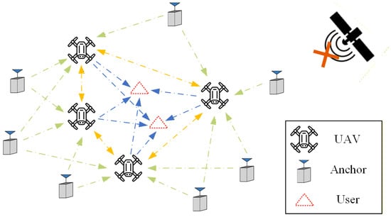
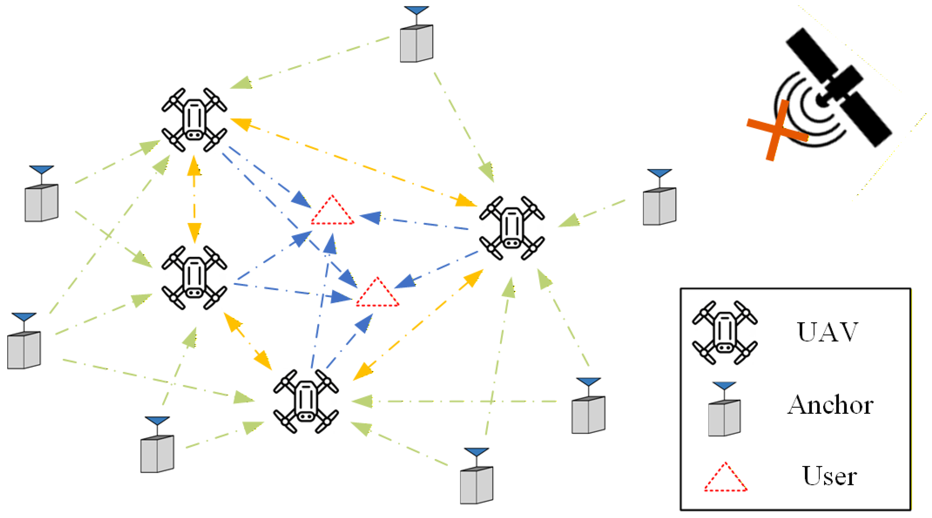
To facilitate subsequent analysis, the system can be abstracted as a directed positioning network. Let $A={\left\{a_i\right\}}_{i=1}^I$ denote the $I$ ground anchors with known positions, $W={\left\{w_j\right\}}_{j=1}^J$ represent the $J$ UAVs, and $U={\left\{u_k\right\}}_{k=1}^K$ represent the $K$ users. Directed edges indicate possible unidirectional pseudorange measurements: from anchors to UAVs, from UAVs to users, and bidirectionally between UAVs. The schematic of this air–ground cooperative scenarios is illustrated in Figure 1.

Figure 1. Typical scenario of UAV-PNS. Where the one-way green arrow indicates the observation from the ground anchor to the UAVs, the one-way blue arrow indicates the observation from the UAVs to the users, and the two-way yellow arrow indicates the mutual observation between the UAVs.

2.2. The Positioning Model and Geometry Indicator

In the basic, the pseudorange measurement model in Single-Point Positioning (SPP) [2] can be suited as follows:

$$\tilde{P}=P+\epsilon =\rho +c\mathrm{\Delta }{t}_r-c\mathrm{\Delta }{t}_t+\epsilon$$

(1)

where $\tilde{P}$ and $P$ are the measured pseudorange and real pseudorange received by the receiver, $\rho$ is the real Euclidean distance between transmitter and receiver, $\mathrm{\Delta }{t}_r$ and $\mathrm{\Delta }{t}_t$ are the clock offsets compared to the system reference time for the transmitter and receiver, respectively, $c$ is the speed of light, and $\epsilon$ is the pseudorange measurement noise. Without loss of generality, we assume that all measurement noises follow a Gaussian distribution.

Thus, we can form all of the observation equations as follows:

$$\left\{\begin{array}{cc}\hfill {\tilde{P}}_{a_1,w_1}& ={\rho }_{a_1,w_1}+c\mathrm{\Delta }{t}_{w_1}-c\mathrm{\Delta }{t}_{a_1}+{\epsilon }_{a_1,w_1}\hfill \\ & ⋮\hfill \\ \hfill {\tilde{P}}_{a_I,w_J}& ={\rho }_{a_I,w_J}+c\mathrm{\Delta }{t}_{w_J}-c\mathrm{\Delta }{t}_{a_I}+{\epsilon }_{a_I,w_J}\hfill \\ \hfill {\tilde{P}}_{w_2,w_1}& ={\rho }_{w_2,w_1}+c\mathrm{\Delta }{t}_{w_1}-c\mathrm{\Delta }{t}_{w_2}+{\epsilon }_{w_2,w_1}\hfill \\ & ⋮\hfill \\ \hfill {\tilde{P}}_{w_{J-1},w_J}& ={\rho }_{w_{J-1},w_J}+c\mathrm{\Delta }{t}_{w_J}-c\mathrm{\Delta }{t}_{w_{J-1}}+{\epsilon }_{w_{J-1},w_J}\hfill \\ \hfill {\tilde{P}}_{w_1,u_1}& ={\rho }_{w_1,u_1}+c\mathrm{\Delta }{t}_{u_1}-c\mathrm{\Delta }{t}_{w_1}+{\epsilon }_{w_1,u_1}\hfill \\ & ⋮\hfill \\ \hfill {\tilde{P}}_{w_J,u_K}& ={\rho }_{w_J,u_K}+c\mathrm{\Delta }{t}_{u_K}-c\mathrm{\Delta }{t}_{w_J}+{\epsilon }_{w_J,u_K}\hfill \end{array}\right.$$

(2)

where ${\tilde{P}}_{a_1,w_1},\dots ,{\tilde{P}}_{a_I,w_J}$ are the pseudorange observations received by UAVs $W={\left\{w_j\right\}}_{j=1}^J$ from ground anchors $A={\left\{a_i\right\}}_{i=1}^I$, ${\tilde{P}}_{w_2,w_1},\dots ,{\tilde{P}}_{w_{J-1},w_J}$ are the pseudorange observations among the UAVs, and ${\tilde{P}}_{w_1,u_1},\dots ,{\tilde{P}}_{w_J,u_K}$ are the pseudorange observations received by users $U={\left\{u_k\right\}}_{k=1}^K$ from UAVs $W={\left\{w_j\right\}}_{j=1}^J$. The pseudorange measurement noises are distributed as ${\epsilon }_{a_i,w_j}~\mathcal{N}\left(0,{\sigma }_{a_i,w_j}^2\right),{\epsilon }_{w_{j-1},w_j}~\mathcal{N}\left(0,{\sigma }_{w_{j-1},w_j}^2\right),{\epsilon }_{w_j,u_k}~\mathcal{N}\left(0,{\sigma }_{w_j,u_k}^2\right)$. This paper adopts the East–North–Up (ENU) coordinate system, where $x$, $y$, and $z$ represent the east, north, and up coordinates, respectively. A well-defined and simple transformation exists between different coordinate systems [3], ensuring that the choice of coordinate system does not affect the positioning results.

The vector to be estimated includes the three-dimensional positions and clock offsets of all of the UAVs and users. Since the above measurement models are instantaneous, there are a total of $4J+4K$ estimable variables at each epoch. The vector to be estimated is shown as follows:

$$\begin{array}{c}\theta =\left[\begin{array}{ccc}\begin{array}{cccc}{x}_{w_1}& y_{w_1}& z_{w_1}& c\mathrm{\Delta }{t}_{w_1}\end{array}& \dots & \begin{array}{cccc}{x}_{w_J}& y_{w_J}& z_{w_J}& c\mathrm{\Delta }{t}_{w_J}\end{array}\end{array}\right.\\ {\left.\begin{array}{ccc}\begin{array}{cccc}{x}_{u_1}& y_{u_1}& z_{u_1}& c\mathrm{\Delta }{t}_{u_1}\end{array}& \dots & \begin{array}{cccc}{x}_{u_K}& y_{u_K}& z_{u_K}& c\mathrm{\Delta }{t}_{u_K}\end{array}\end{array}\right]}^{\mathrm{T}}\end{array}$$

(3)

Combining the vector to be estimated, by analogy with SPP, and performing a first-order Taylor expansion on the observation equation in the linearized position of ${\theta }^0$ [2], a linearized positioning equation can be obtained as follows:

$$b+\epsilon =Hd\theta$$

(4)

where $d\theta$ is the corrections, $H$ is the overall Jacobi matrix, and $b$ is the observation vector, the details of these matrices and vectors will be elaborated in the next section. While solving the problem with algorithm in minimize the residual sum of squares ${\epsilon }^{\mathrm{T}}\epsilon$, then:

$$d\theta ={\left(H^{T}WH\right)}^{-1}{H}^{T}Wb$$

(5)

where the $W$ is the weight matrix, $W={\left({\epsilon }^{\mathrm{T}}\epsilon \right)}^{-1}$. Therefore, the covariance in the resolution estimated $\widehat{\theta }$ is:

$$\begin{array}{l}\mathrm{cov}(\delta \widehat{\theta })=\mathbb{E}\left({\left(H^{\mathrm{T}}WH\right)}^{-1}{H}^{\mathrm{T}}W\epsilon {\left({\left(H^{\mathrm{T}}WH\right)}^{-1}{H}^{\mathrm{T}}W\epsilon \right)}^{\mathrm{T}}\right)\\ =\mathbb{E}\left({\left(H^{\mathrm{T}}WH\right)}^{-1}{H}^{\mathrm{T}}W\epsilon {\epsilon }^{\mathrm{T}}WH{\left(H^{\mathrm{T}}WH\right)}^{-1}\right)\\ ={\left(H^{\mathrm{T}}WH\right)}^{-1}\end{array}$$

(6)

It can be regarded as a mapping matrix from the noise covariance observed within the network to the vector to be estimated, determined the error amplification gain.

2.3. Lightweight Computing

This section first details the structure of the Jacobian matrix $H$ and the observation vector $b$. It then proposes a decomposition-based method for evaluating user geometric precision, aimed at significantly reducing computational complexity.

Viewed along its rows and columns, the Jacobian matrix $H$ exhibits a clear block structure: the rows represent observations grouped into three categories, anchor-to-UAV, UAV-to-UAV, and UAV-to-user, while the columns correspond to the unknown states partitioned into UAV positions and user positions. Hence, we split $H$ and $b$ as follows:

$$H=\left[\begin{array}{cc}{H}_W^A& 0\\ H_W^W& 0\\ H_W^U& H_U^W\end{array}\right],b=\left[\begin{array}{c}{b}_W^A\\ b_W^W\\ b_U^W\end{array}\right]$$

(7)

where $H_W^A$ denotes the collective Jacobian submatrix corresponding to all anchor-to-UAV observations, $H_W^W$ the submatrix for all UAV-to-UAV observations, $H_U^W$ and $H_W^U$ the submatrices for all UAV-to-user observations, and $b_W^A$, $b_W^W$ and $b_U^W$ are the corresponding measurement residual vectors. The detailed composition of these blocks is given as follows:

$$H_W^A=\left[\begin{array}{cccc}{H}_{w_1}^{A_1}& 0& \cdots & 0\\ 0& H_{w_2}^{A_2}& \cdots & 0\\ ⋮& ⋮& \ddots & 0\\ 0& 0& 0& H_{w_J}^{A_J}\end{array}\right],b=\left[\begin{array}{c}{b}_{w_1}^{A_1}\\ b_{w_2}^{A_2}\\ ⋮\\ b_{w_J}^{A_J}\end{array}\right]$$

(8)

$$H_{w_j}^{A_j}=\left[\begin{array}{cccc}{\displaystyle \frac{x_{w_j}^0-x_{a_1}}{{\rho }_{a_1,w_j}^0}}& {\displaystyle \frac{y_{w_j}^0-y_{a_1}}{{\rho }_{a_1,w_j}^0}}& {\displaystyle \frac{z_{w_j}^0-z_{a_1}}{{\rho }_{a_1,w_j}^0}}& 1\\ {\displaystyle \frac{x_{w_j}^0-x_{a_2}}{{\rho }_{a_2,w_j}^0}}& {\displaystyle \frac{y_{w_j}^0-y_{a_2}}{{\rho }_{a_2,w_j}^0}}& {\displaystyle \frac{z_{w_j}^0-z_{a_2}}{{\rho }_{a_2,w_j}^0}}& 1\\ ⋮& ⋮& ⋮& ⋮\\ {\displaystyle \frac{x_{w_j}^0-x_{a_I}}{{\rho }_{a_I,w_j}^0}}& {\displaystyle \frac{y_{w_j}^0-y_{a_I}}{{\rho }_{a_I,w_j}^0}}& {\displaystyle \frac{z_{w_j}^0-z_{a_I}}{{\rho }_{a_I,w_j}^0}}& 1\end{array}\right],b_{w_j}^{A_j}=\left[\begin{array}{c}{P}_{a_1,w_j}-{\rho }_{a_1,w_j}^0+c\mathrm{\Delta }{t}_{a_1}\\ P_{a_2,w_j}-{\rho }_{a_2,w_j}^0+c\mathrm{\Delta }{t}_{a_2}\\ ⋮\\ P_{a_I,w_j}-{\rho }_{a_I,w_j}^0+c\mathrm{\Delta }{t}_{a_I}\end{array}\right]$$

(9)

where $H_{w_j}^{A_j}$ and $b_{w_j}^{A_j}$ are the Jacobian submatrix and residual vector associated with the observations received by the $j$-th UAV $w_j$ from their received anchor set $A_j\in A={\left\{a_i\right\}}_{i=1}^I$. Each row of $H_{w_j}^{A_j}$ corresponds to the line-of-sight (LOS) unit vector (augmented with a clock bias component) from $w_j$ to the respective anchor.

$$H_W^W=\left[\begin{array}{cccc}{H}_{w_1}^{W_1}& -h_{w_1}^{w_2}& \cdots & -h_{w_1}^{w_j}\\ -h_{w_2}^{w_1}& H_{w_2}^{W_2}& \cdots & -h_{w_2}^{w_j}\\ ⋮& ⋮& \ddots & ⋮\\ -h_{w_j}^{w_1}& -h_{w_j}^{w_2}& \cdots & H_{w_j}^{W_j}\end{array}\right],b=\left[\begin{array}{c}{b}_{w_1}^{W_1}\\ b_{w_2}^{W_2}\\ ⋮\\ b_{w_j}^{W_j}\end{array}\right]$$

(10)

$$H_{w_j}^{W_j}=\left[\begin{array}{cccc}{\displaystyle \frac{x_{w_j}^0-x_{w_1}^0}{{\rho }_{w_1,w_j}^0}}& {\displaystyle \frac{y_{w_j}^0-y_{w_1}^0}{{\rho }_{w_1,w_j}^0}}& {\displaystyle \frac{z_{w_j}^0-z_{w_1}^0}{{\rho }_{w_1,w_j}^0}}& 1\\ ⋮& ⋮& ⋮& ⋮\\ {\displaystyle \frac{x_{w_j}^0-x_{w_J}^0}{{\rho }_{w_J,w_j}^0}}& {\displaystyle \frac{y_{w_j}^0-y_{w_J}^0}{{\rho }_{w_J,w_j}^0}}& {\displaystyle \frac{z_{w_j}^0-z_{w_J}^0}{{\rho }_{w_J,w_j}^0}}& 1\end{array}\right],b_{w_j}^{W_j}=\left[\begin{array}{c}{P}_{w_1,w_j}-{\rho }_{w_1,w_j}^0\\ ⋮\\ P_{w_{j-1},w_j}-{\rho }_{w_{j-1},w_j}^0\\ P_{w_{j+1},w_j}-{\rho }_{w_{j+1},w_J}^0\\ ⋮\\ P_{w_J,w_j}-{\rho }_{w_J,w_j}^0\end{array}\right]$$

(11)

$$h_{w_j}^{w_m}=\left[\begin{array}{cccc}0& 0& 0& 0\\ ⋮& ⋮& ⋮& ⋮\\ {\displaystyle \frac{x_{w_j}^0-x_{w_m}^0}{{\rho }_{w_m,w_j}^0}}& {\displaystyle \frac{y_{w_j}^0-y_{w_m}^0}{{\rho }_{w_m,w_j}^0}}& {\displaystyle \frac{z_{w_j}^0-z_{w_m}^0}{{\rho }_{w_m,w_j}^0}}& 1\\ ⋮& ⋮& ⋮& ⋮\\ 0& 0& 0& 0\end{array}\right]$$

(12)

where $H_{w_j}^{W_j}$ and $b_{w_j}^{W_j}$ are the Jacobian submatrix and residual vector for the observations received by the $j$-th UAV $w_j$ from the other UAVs, form the set of $W_j\in W={\left\{w_j\right\}}_{j=1}^J$. Each row corresponds to the LOS unit vector from $w_j$ to the transmitting UAV $w_m\left(m\le J\hspace{0.33em}\mathrm{and}\hspace{0.33em}m\ne j\right)$. The individual row vector $h_{w_j}^{w_m}$ is a sparse row with only the entries corresponding to the state of $w_m$ being non-zero, and it is identical to the $m$-th observed row within the full block $H_{w_j}^{W_j}$, form the equation $H_{w_j}^{W_j}={\displaystyle \sum _m^{1,\dots ,j-1,j+1,\dots ,J}{h}_{w_j}^{w_m}}$.

$$H_W^U=\left[\begin{array}{cccc}-h_{u_1}^{w_1}& -h_{u_1}^{w_2}& \cdots & -h_{u_1}^{w_j}\\ -h_{u_2}^{w_1}& -h_{u_2}^{w_2}& \cdots & -h_{u_2}^{w_j}\\ ⋮& ⋮& \ddots & ⋮\\ -h_{u_K}^{w_1}& -h_{u_K}^{w_2}& \cdots & -h_{u_K}^{w_j}\end{array}\right],H_U^W=\left[\begin{array}{cccc}{H}_{u_1}^{W_1}& 0& \cdots & 0\\ 0& H_{u_2}^{W_2}& \cdots & 0\\ ⋮& ⋮& \ddots & ⋮\\ 0& 0& \cdots & H_{u_K}^{W_K}\end{array}\right],b_U^W=\left[\begin{array}{c}{b}_{u_1}^{W_1}\\ b_{u_2}^{W_2}\\ ⋮\\ b_{u_K}^{W_K}\end{array}\right]$$

(13)

$$H_{u_k}^{W_k}=\left[\begin{array}{cccc}{\displaystyle \frac{x_{u_k}^0-x_{w_1}^0}{{\rho }_{w_1,u_k}^0}}& {\displaystyle \frac{y_{u_k}^0-y_{w_1}^0}{{\rho }_{w_1,u_k}^0}}& {\displaystyle \frac{z_{u_k}^0-z_{w_1}^0}{{\rho }_{w_1,u_k}^0}}& 1\\ {\displaystyle \frac{x_{u_k}^0-x_{w_2}^0}{{\rho }_{w_2,u_k}^0}}& {\displaystyle \frac{y_{u_k}^0-y_{w_2}^0}{{\rho }_{w_2,u_k}^0}}& {\displaystyle \frac{z_{u_k}^0-z_{w_2}^0}{{\rho }_{w_2,u_k}^0}}& 1\\ ⋮& ⋮& ⋮& ⋮\\ {\displaystyle \frac{x_{u_k}^0-x_{w_J}^0}{{\rho }_{w_J,u_k}^0}}& {\displaystyle \frac{y_{u_k}^0-y_{w_J}^0}{{\rho }_{w_J,u_k}^0}}& {\displaystyle \frac{z_{u_k}^0-z_{w_J}^0}{{\rho }_{w_J,u_k}^0}}& 1\end{array}\right],b_{u_k}^{W_k}=\left[\begin{array}{c}{P}_{w_1,u_k}-{\rho }_{w_1,u_k}^0\\ P_{w_2,u_k}-{\rho }_{w_2,u_k}^0\\ ⋮\\ P_{w_J,u_k}-{\rho }_{w_J,u_k}^0\end{array}\right]$$

(14)

$$h_{u_k}^{w_j}=\left[\begin{array}{cccc}0& 0& 0& 0\\ ⋮& ⋮& ⋮& ⋮\\ {\displaystyle \frac{x_{u_k}^0-x_{w_j}^0}{{\rho }_{w_j,u_k}^0}}& {\displaystyle \frac{y_{u_k}^0-y_{w_j}^0}{{\rho }_{w_j,u_k}^0}}& {\displaystyle \frac{z_{u_k}^0-z_{w_j}^0}{{\rho }_{w_j,u_k}^0}}& 1\\ ⋮& ⋮& ⋮& ⋮\\ 0& 0& 0& 0\end{array}\right]$$

(15)

where $H_{u_k}^{W_k}$ and $b_{u_k}^{W_k}$ are the Jacobian submatrix and residual vector for the observations received by the k-th user $u_k$ from its received UAVs $W_k\in W={\left\{w_j\right\}}_{j=1}^J$. Each row of $H_{u_k}^{W_k}$ represents the LOS unit vector from $u_k$ to the corresponding transmitting UAV. The individual row vector $h_{u_k}^{w_j}$ is sparse, with only the entries corresponding to the state of $w_j$ being non-zero, and matches the n-th row of $H_{u_k}^{W_k}$; thus, we have $H_{u_k}^{W_k}={\displaystyle \sum _{j=1}^J{h}_{u_k}^{w_j}}$.

Back to Equation (6), it evaluated the global nodes in geometry configurations, but sometimes we only need part of the nodes, for users, as an instance. The dimension of $H^{\mathrm{T}}WH\in {ℝ}^{\left(4J+4K\right)\times \left(4J+4K\right)}$ will increase rapidly with the expansion of nodes, and the inverse operation will result in a severe computational load. Based on the block characteristics of the overall observation matrix $H$, we have:

$$\begin{array}{cc}{\left(H^{\mathrm{T}}WH\right)}^{-1}& ={\left\{\left[\begin{array}{ccc}{H_W^A}^{\mathrm{T}}& {H_W^W}^{\mathrm{T}}& {H_W^U}^{\mathrm{T}}\\ 0& 0& {H_U^W}^{\mathrm{T}}\end{array}\right]\left[\begin{array}{ccc}{W}_W^A& 0& 0\\ 0& W_W^W& 0\\ 0& 0& W_U^W\end{array}\right]\left[\begin{array}{cc}{H}_W^A& 0\\ H_W^W& 0\\ H_W^U& H_U^W\end{array}\right]\right\}}^{-1}\hfill \\ & ={\left[\begin{array}{cc}{H_W^A}^{\mathrm{T}}{W}_W^A{H}_W^A+{H_W^W}^{\mathrm{T}}{W}_W^W{H}_W^W+{H_W^U}^{\mathrm{T}}{W}_U^W{H}_W^U& {H_W^U}^{\mathrm{T}}{W}_U^W{H}_U^W\\ {H_U^W}^{\mathrm{T}}{W}_U^W{H}_W^U& {H_U^W}^{\mathrm{T}}{W}_U^W{H}_U^W\end{array}\right]}^{-1}\hfill \\ & =\left[\begin{array}{cc}{G}_W& G_{12}\\ G_{21}& G_U\end{array}\right]\hfill \end{array}$$

(16)

Use the Schur complement to avoid direct large-scale inversion. In most practical scenarios, we only need to compute the two main diagonal block matrices in Equation (16) as they directly encapsulate the geometric precision factors for the UAVs and the users, respectively. The corresponding Schur complement is given by:

$$\begin{array}{l}{G}_W=\left({H_W^A}^{\mathrm{T}}{W}_W^A{H}_W^A+{H_W^W}^{\mathrm{T}}{W}_W^W{H}_W^W+{H_W^U}^{\mathrm{T}}{W}_U^W{H}_W^U-\right.\\ {\left.{H_W^U}^{\mathrm{T}}{W}_U^W{H}_U^W{\left({H_U^W}^{\mathrm{T}}{W}_U^W{H}_U^W\right)}^{-1}{H_U^W}^{\mathrm{T}}{W}_U^W{H}_W^U\right)}^{-1}\end{array}$$

(17)

$$\begin{array}{l}{G}_U=\left({H_U^W}^{\mathrm{T}}{W}_U^W{H}_U^W-\right.\\ {\left.{H_U^W}^{\mathrm{T}}{W}_U^W{H}_W^U{\left({H_W^A}^{\mathrm{T}}{W}_W^A{H}_W^A+{H_W^W}^{\mathrm{T}}{W}_W^W{H}_W^W+{H_W^U}^{\mathrm{T}}{W}_U^W{H}_W^U\right)}^{-1}{H_W^U}^{\mathrm{T}}{W}_U^W{H}_U^W\right)}^{-1}\\ =\left({H_U^W}^{\mathrm{T}}\left(W_U^W\right.-\right.\\ {\left.\left.W_U^W{H}_W^U{\left({H_W^A}^{\mathrm{T}}{W}_W^A{H}_W^A+{H_W^W}^{\mathrm{T}}{W}_W^W{H}_W^W+{H_W^U}^{\mathrm{T}}{W}_U^W{H}_W^U\right)}^{-1}{H_W^U}^{\mathrm{T}}{W}_U^W\right)H_U^W\right)}^{-1}\end{array}$$

(18)

So, (18) is exactly what we want to evaluate the users’ geometry configurations, and $G_U$ is defined as the comprehensive DOP matrix. The computational complexity is reduced from $\mathcal{O}\left({\left(4J+4K\right)}^3\right)$ to $\mathcal{O}\left({\left(4J\right)}^3\right)$.

3. UAV Swarm Route Planning

This section develops the proposed APF framework for autonomous UAV swarm trajectory planning. It begins with the principle of the algorithm, followed by the construction of the composite potential field using the geometric evaluation metric from Section 2 as the attractive component and operational constraints as repulsive terms. The derivation of the resulting virtual forces, including a lightweight finite-difference approximation for gradients, is then presented to enable real-time motion control.

3.1. Principle of Algorithm

The Artificial Potential Field (APF) method, originally proposed by Khatib in 1986 [23], is a classical reactive approach for real-time path planning and motion control of robotic agents. By analogy with physical potential fields, the method models the environment and task objectives through virtual attractive and repulsive forces. The resultant force, computed as the negative gradient of the total artificial potential, directly guides the agent toward the goal while avoiding obstacles or undesirable configurations. Over the past decades, APF and its numerous variants have been widely applied to multi-agent coordination, UAV trajectory planning, and swarm robotics, owing to its conceptual simplicity, extremely low computational cost per control cycle, and natural suitability for distributed implementation [24,25].

Despite its advantages, the classical APF suffers from well-known limitations, most notably the susceptibility to local minima, oscillations in narrow passages, and goal non-reachability under certain configurations [26]. In recent years, various improvements have been proposed to mitigate these issues, including harmonic potential fields, virtual force hybrid methods, and adaptive repulsive force functions [25,27].

For the air–terrestrial cooperative positioning problem considered in this paper, the classical APF remains highly attractive for the following reasons: First, the primary objective is to continuously optimize the geometric configuration of the UAV swarm in response to dynamic and heterogeneous user demands, rather than to guarantee convergence to a globally optimal static formation. Second, the onboard computational resources of UAVs are strictly limited, making lightweight, reactive methods far more practical than global optimization techniques such as evolutionary algorithms or convex solvers. Third, the geometric evaluation metric derived in Section 2.2 is naturally differentiable and can be directly used to construct the potential field, enabling a seamless bridge between high-level positioning performance and low-level motion commands. These characteristics make APF particularly well-suited as a real-time, trajectory adaptation framework for the UAV swarm in this context.

Consequently, rather than proposing a new variant to address the local minima issue of APF itself, this work focuses on the specific application of the classical APF to the UAV swarm route planning problem in air–ground collaborative radio navigation systems. The emphasis is placed on how to properly define the potential field using the proposed geometry evaluation model so as to achieve effective real-time optimization of user-end positioning accuracy under dynamic conditions.

3.2. Establish of Artificial Potential Field

The total Artificial Potential Field $U_{\mathrm{total}}$ is constructed as the superposition of an attractive potential $U_{\mathrm{att}}$ and multiple repulsive potentials $U_{\mathrm{rep},i}$:

$$U_{\mathrm{total}}=U_{\mathrm{att}}+{\displaystyle \sum _{i=1}^M{U}_{\mathrm{rep},i}}$$

(19)

where $M$ is the number of active constraints (e.g., altitude limits, terrain, inter-UAV separation). The virtual force is then derived as $F=-\nabla U_{\mathrm{total}}$ (detailed in Section 3.3). This formulation ensures that UAVs are continuously pulled toward geometries minimizing user positioning error while pushed away from infeasible regions.

The primary objective is to minimize the users’ comprehensive DOP $G_U$. The attractive potential is defined as follows: $U_{\mathrm{att}}=\mathrm{tr}\left(G_U\right)$

$$U_{\mathrm{att}}=\alpha \mathrm{tr}\left(G_U\right)$$

(20)

where $\alpha$ is the coefficient factor. The negative gradient $\nabla U_{\mathrm{att}}$ naturally guides UAVs downhill toward swarm geometries that optimize end-to-end user accuracy, bridging high-level precision mapping with reactive control. Unlike discrete DOP-map waypoint methods, this continuous, differentiable formulation enables real-time, gradient-based swarm adaptation to dynamic heterogeneous users.

Repulsive potentials address key operational constraints, modeled with the standard inverse-distance form to decay rapidly away from hazards:

$$U_{\mathrm{rep},i}=\left\{\begin{array}{ll}{\eta }_i{\displaystyle \frac{1}{{d_i}^2}},\hfill & d_i\le d_{0,i}\hfill \\ 0,\hfill & d_i>d_{0,i}\hfill \end{array}\right.$$

(21)

where $d_i$ is the distance to the i-th constraint boundary, $d_{0,i}$ the influence range, and ${\eta }_i>0$ the gain. Specific forms include:

(1)

Minimum altitude constraint: $d_1=z-h_{\min }$, where $h_{\min }>0$. This ensures $z>h_{\min }$, preventing collisions with uneven ground or obstacles.

(2)

Inter-UAV collision avoidance: for UAV j and peer m, $d_2=\Vert p_j-p_m\Vert -r_{\mathrm{safe}}$, with $r_{\mathrm{safe}}$ of the safety radius.

(3)

Boundary of zones: $d_3$ from polygonal boundaries. Parameters $\{{\eta }_i,d_{0,i}\}$ are selected empirically to dominate near boundaries.

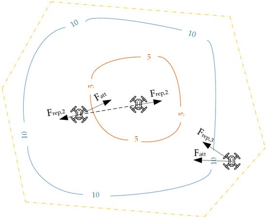
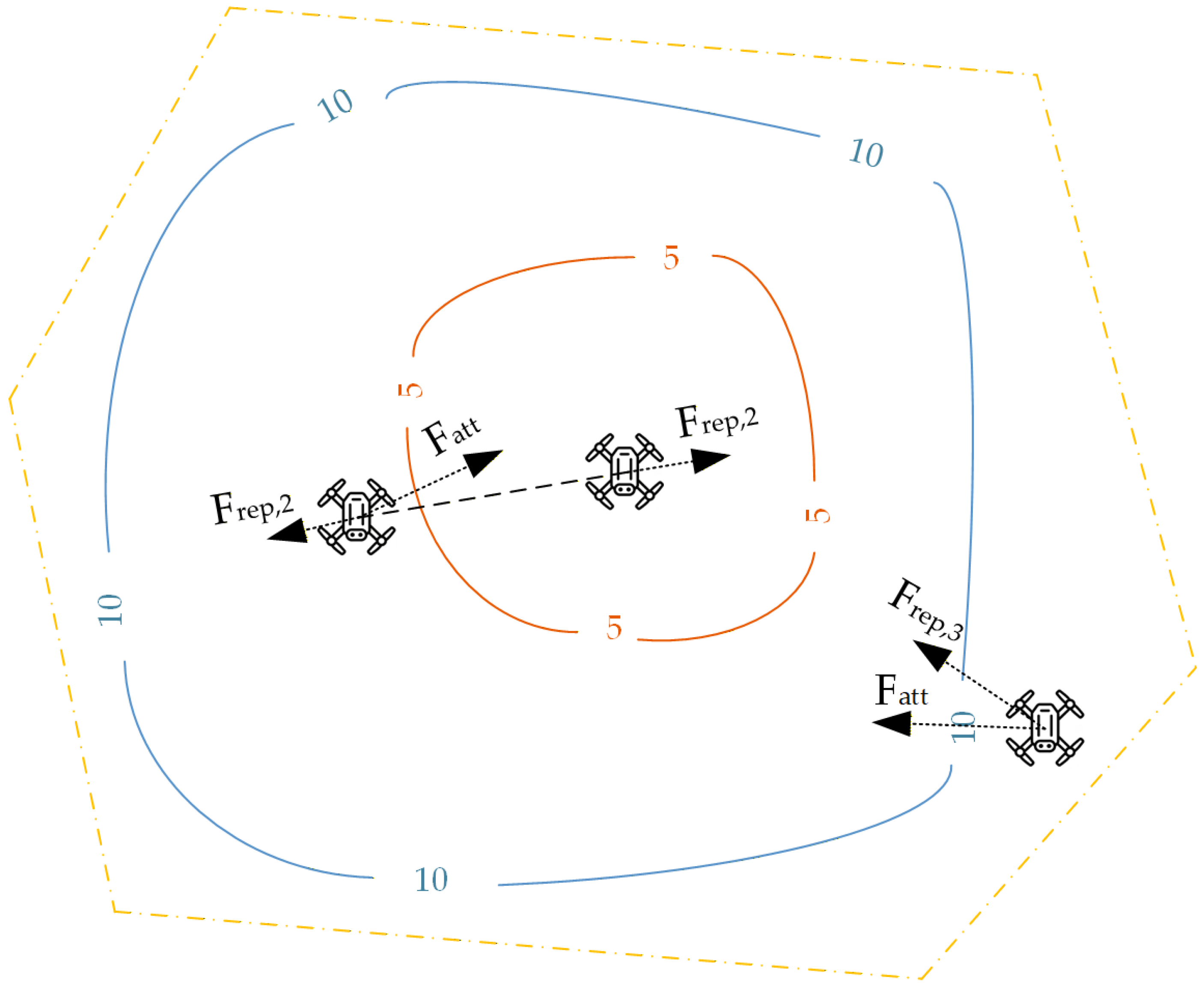
Figure 2 illustrates the composite field, where low-DOP valleys attract the swarm while repulsive barriers enforce safety. The red and blue contour lines represent the spatial variation in the comprehensive DOP levels, and the yellow dashed line is the boundary.

Figure 2. APF for UAV swarm.

3.3. Derivation of UAV Virtual Force

The virtual force acting on each UAV is derived from the negative gradient of the total Artificial Potential Field established in Section 3.2. For the j-th UAV, the force is given by:

$$F_j=-\nabla U_{\mathrm{total}}=-\nabla U_{\mathrm{att}}-{\displaystyle \sum _{i=1}^M\nabla }{U}_{\mathrm{rep},i}$$

(22)

where $\nabla ={[\partial /\partial x_j,\partial /\partial y_j,\partial /\partial z_j]}^{\mathrm{T}}$ denotes the spatial gradient operator. This resultant force guides the UAV’s motion via simple kinematic integration (e.g., $v_j\leftarrow v_j+\mathrm{\Delta }t\cdot F_j/m_j$, followed by position update), enabling reactive trajectory adaptation. Below, we derive the gradients for the attractive and repulsive components, prioritizing computational efficiency for onboard implementation.

The attractive potential $U_{\mathrm{att}}$ is a scalar function of the entire swarm configuration. The partial derivation of $U_{\mathrm{att}}$ to the coordinate of j-th UAV $r_{w_j}={\left[x_{w_j},y_{w_j},z_{w_j}\right]}^{\mathrm{T}}$ is the virtual force. While the analytical expression can be obtained by differentiating the $G_U$, this would require complex matrix derivatives that increase computational burden in high-dimensional settings.

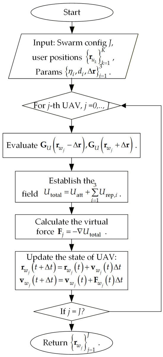
To maintain the lightweight nature of our framework and ensure real-time feasibility on resource-constrained UAV platforms, we employ a finite-difference approximation for the gradient:

$$\nabla U_{\mathrm{att}}\approx {\displaystyle \frac{G_U(r_{w_j}+\mathrm{\Delta }r)-G_U(r_{w_j}-\mathrm{\Delta }r)}{2\mathrm{\Delta }r}}$$

(23)

where $\mathrm{\Delta }r$ is a small perturbation along the three axis. The finite-difference approximation for gradients is a widely adopted practical approach in APF, as demonstrated in prior works for real-time path planning [28,29]. This central difference scheme requires only six evaluations of the scalar $G_U$ function per UAV per control cycle, preserving low complexity while providing sufficient accuracy for trajectory guidance. Numerical stability is ensured by adaptive $\mathrm{\Delta }$ scaling based on UAV speed or DOP magnitude. For offline analysis or higher precision, the analytical gradient can be derived as detailed in Appendix A.

The repulsive gradients are analytically straightforward due to their simple inverse-distance form Equation (21). For a general repulsive term $U_{\mathrm{rep},i}={\eta }_i/{d_i}^2$ (active when $d_i\le d_{0,i}$), the gradient is:

$$\nabla U_{\mathrm{rep},i}=-{\eta }_i{\displaystyle \frac{u_i}{2{d_i}^3}}$$

(24)

where $u_i$ is the unit direction vector from $r_{w_j}$ toward the constraint boundary (e.g., upward for altitude: $u_1={[0,0,1]}^{\mathrm{T}}$; toward peer UAV m for collision: $u_2=(r_{w_m}-r_{w_j})/\Vert r_{w_m}-r_{w_j}\Vert$). This closed-form expression incurs negligible computation, complementing the attractive component’s approximation.

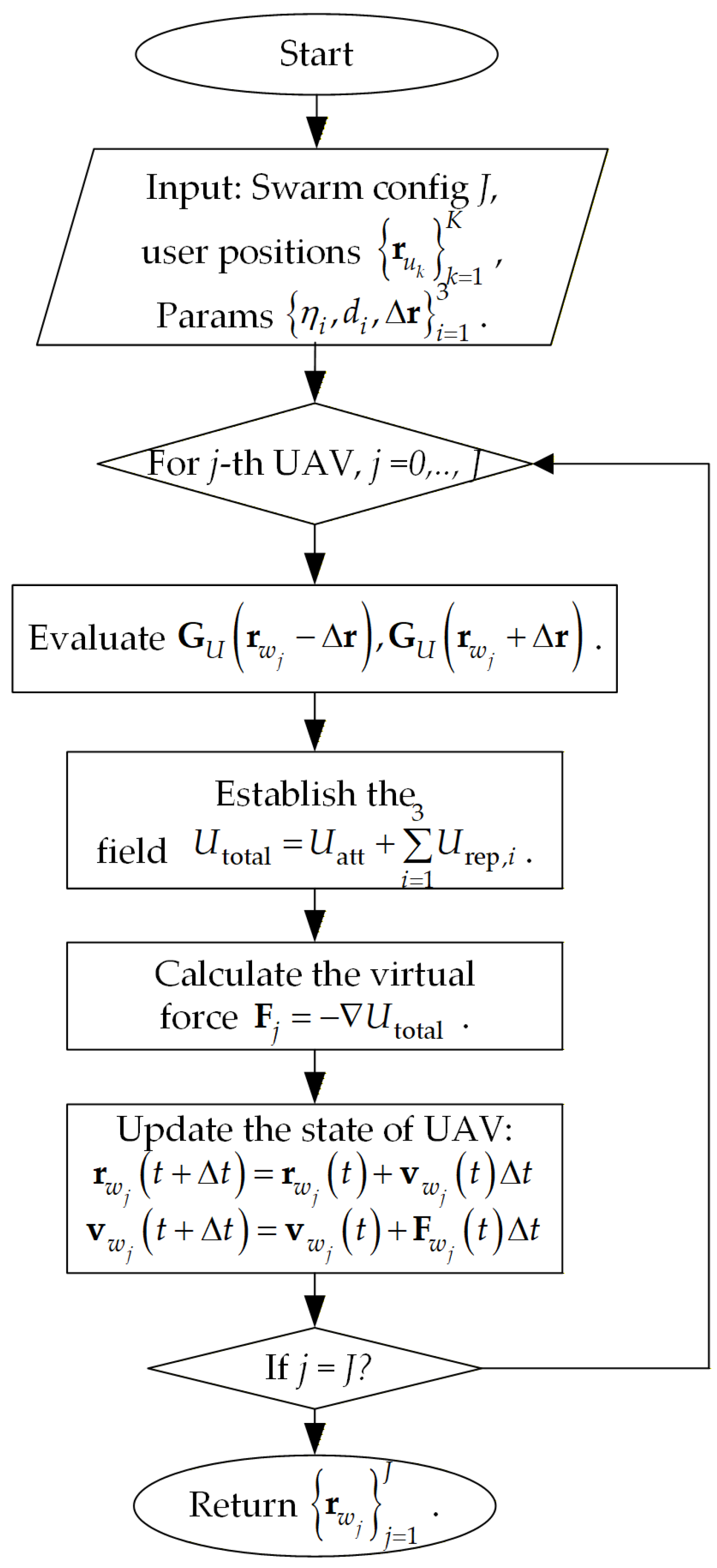
Figure 3 summarizes the overall UAV swarm route planning algorithm.

Figure 3. The flow of the algorithm.

It should be noted that while each UAV computes local forces reactively, the global user GDOP scalar is aggregated by a lightweight central coordinator (e.g., lead UAV or ground station) and periodically broadcast to the swarm via low-latency links, enabling consistent geometry optimization without requiring full observation sharing at every step.

4. Simulation

This section evaluates the effectiveness and performance of the proposed framework through comprehensive simulations. It first examines a static scenario to verify convergence and baseline geometric improvement, and then extends to dynamic scenarios with piecewise linear user motion to demonstrate real-time adaptability and robustness. Comparative analyses against non-adaptive baselines highlight the algorithm’s superior user accuracy, inter-user balance, and temporal stability under varying conditions.

4.1. Static Scenarios

To validate the basic convergence and effectiveness of the proposed APF-based UAV swarm route planning framework, a static scenario is first considered. In this setup, ground users remain fixed in position throughout the simulation, allowing us to isolate the algorithm’s ability to drive the UAV swarm from suboptimal initial configurations toward geometries that minimize the user comprehensive GDOP ($G_U$). This serves as a baseline verification of the core mechanism: the attractive potential derived from the Schur-complement-based metric $G_U$ successfully guides the swarm downhill in the potential field, while repulsive potentials enforce operational constraints.

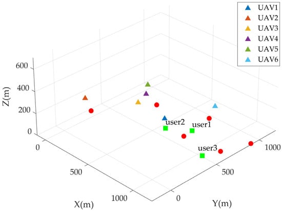
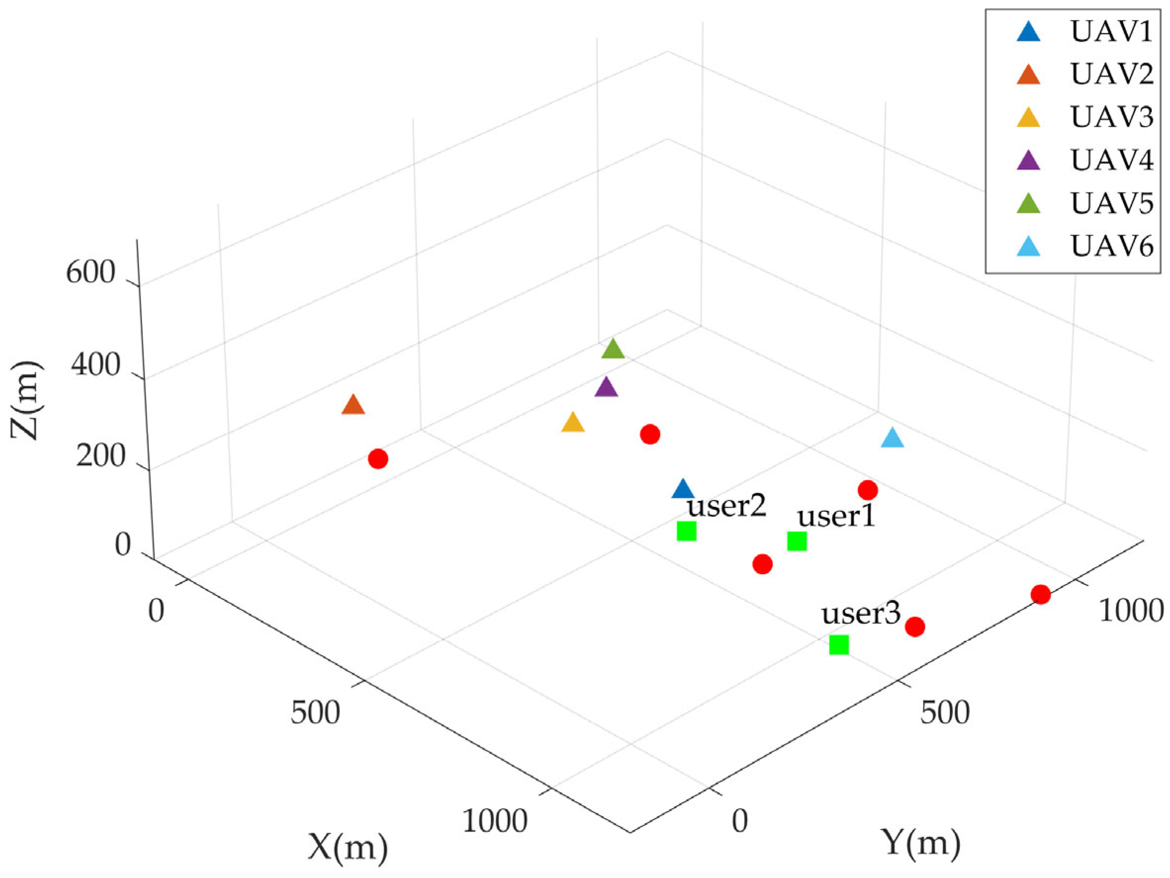
The simulation environment is defined within a cubic spatial region of dimensions $1200 \mathrm{m}\times 1200 \mathrm{m}\times 700 \mathrm{m}$ (i.e., $0<x<1200$, $0<y<1200$, $0<z<700$). Figure 4 illustrates the initial configuration of the system. Six ground anchors (marked as red circles) are deployed at fixed positions on the ground plane ($z=0$) to provide a sparse but sufficient reference network. The six UAVs start from diverse initial positions (represented by triangles of different colors) scattered across the airspace, intentionally including some poor geometric configurations relative to the users. Three ground users are placed at fixed locations (green squares), representing typical static targets in GNSS-denied applications such as monitoring stations or emergency response points.

Figure 4. Initial configuration of the static scenario. Red circles: ground anchors; colored triangles: initial UAV positions; green squares: static users.

Key simulation parameters are selected to reflect realistic UAV platform characteristics and to balance the attractive and repulsive forces. Simulation parameters are shown in Table 1.

Table 1. Simulation parameter settings.

Simulation Parameter	Value
Maximum UAV velocity	15 m/s
Maximum acceleration induced by the total virtual force	8 m/s2
Repulsive potential influence range ($d_{0,1},d_{0,2},d_{0,3}$)	100 m, 100 m, 100 m
Repulsive gain (${\eta }_1={\eta }_2={\eta }_3$)	8
Attractive potential scaling factor ($\alpha$)	400
Finite-difference perturbation distance ($\left|\mathrm{\Delta }r\right|$)	1 m

These values were tuned empirically through preliminary tests to achieve smooth convergence without excessive oscillations or overly aggressive maneuvers. The UAV swarm is updated synchronously with a fixed time step of $\mathrm{\Delta }t=0.1 \mathrm{s}$, and the simulation runs 300 s when most UAVs turn to be converged.

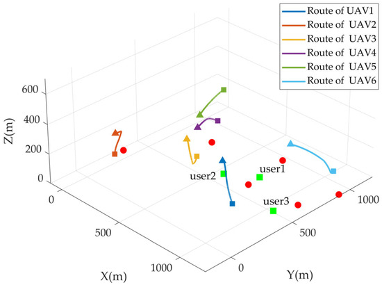
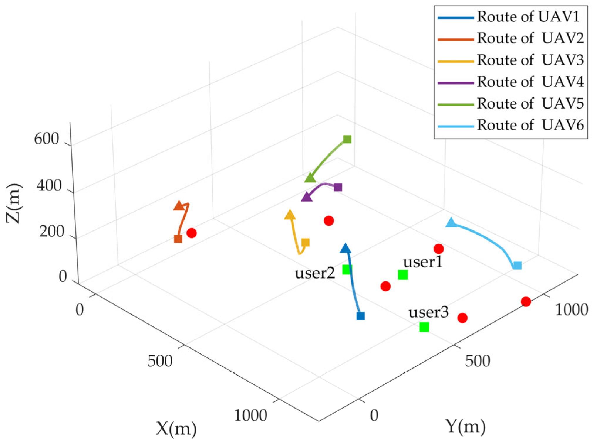
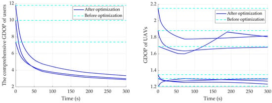
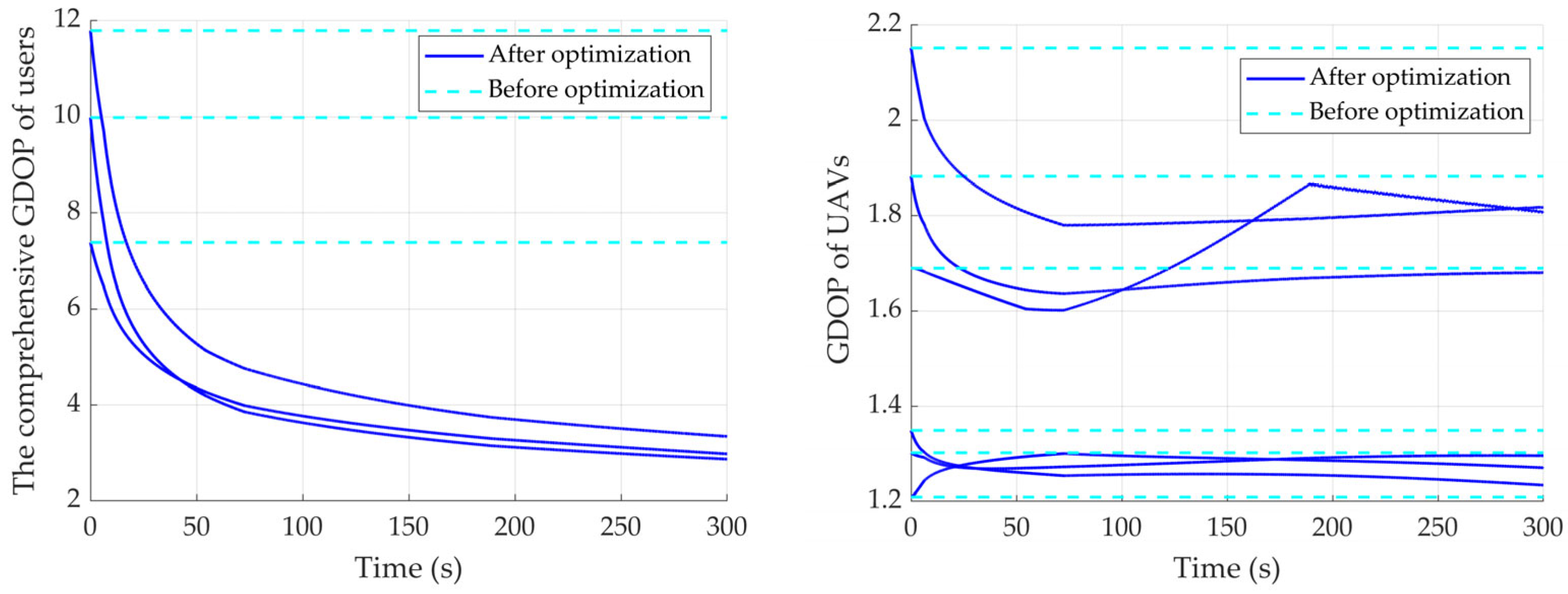
Figure 5 shows the autonomous planned route of the UAV swarm trajectories during the simulation. Starting from the initial poor geometry, the swarm gradually spreads out and ascends, forming a more favorable volumetric configuration relative to the user group. The corresponding evolution of comprehensive GDOP for each user and GDOP for each UAV is plotted in Figure 6.

Figure 5. Autonomous planned route of UAV swarm in the static scenario. Red circles: ground anchors; colored triangles and squares: initial UAV positions and final UAV positions in the mission; green squares: static users.

Figure 6. Evolution of the comprehensive GDOP of users and the GDOP of UAVs over time in the static scenario.

The metric decreases monotonically from an initial value of approximately 10 to about 3, demonstrating stable and rapid convergence. Notice in Figure 6 that, after most UAVs converge, a few still display slow, uniform rectilinear drift. This behavior arises because their positions exert only negligible influence on the user comprehensive GDOP, resulting in a correspondingly balanced virtual force state. This baseline scenario also serves as a reference for subsequent dynamic and comparative experiments, highlighting the algorithm’s intrinsic convergence properties under controlled conditions.

There are two points need to be noted in particular: First, when serving low-altitude users, the GDOP characteristics experienced by these users exhibit strong similarity to those of the UAVs due to the layered measurement structure and comparable altitudes. Second, noise-free and instantaneous access to UAV and user positions for computing the global user GDOP metric: In large-scale outdoor regional navigation, this simplification has limited impact due to geometric redundancy and spatial scale; however, in indoor or NLOS-heavy scenarios, position estimation uncertainties would propagate into the APF gradients and require additional mitigation. When such uncertainties are significant, techniques such as those proposed by Shin et al. [30]—adding a virtual force term to coordinate estimation variance—could be integrated into the total virtual force to enhance robustness.

4.2. Dynamic Scenarios

To evaluate the proposed framework’s ability to handle time-varying user demands in realistic GNSS-denied environments, a dynamic scenario is designed where ground users exhibit piecewise constant-velocity motion over a 600 s simulation horizon. This setup tests the algorithm’s convergence properties, real-time adaptability to user state changes, and overall improvement in user positioning performance compared to a non-adaptive baseline.

The simulation retains the same spatial bounds and anchor/user placement as the static scenario (Figure 4), with six UAVs and three ground users. The total duration of 600 s is divided into three equal segments of 200 s each. At the beginning of each segment ($t=0 \mathrm{s}$, $t=200 \mathrm{s}$, $t=400 \mathrm{s}$), every user is assigned a new constant velocity vector $v_u={[v_x,v_y,v_z]}^{\mathrm{T}}$, where the horizontal components $v_x$ and $v_y$ are independently drawn from a Gaussian distribution $\mathcal{N}(0,{0.15}^2) \mathrm{m}/\mathrm{s}$, and the vertical component $v_z$ is drawn from $\mathcal{N}(0,{0.005}^2) \mathrm{m}/\mathrm{s}$ and then taken as an absolute value ($\left|v_z\right|$) to prevent descent below ground level ($z\ge 0$). This results in each user following a three-segment piecewise linear trajectory (connected broken lines) with sudden velocity changes at the segment boundaries, simulating realistic heterogeneous motion patterns such as pedestrians, vehicles, or monitoring equipment in GNSS-denied areas.

The same APF parameters as in the static case are employed, ensuring consistency across experiments. The UAV swarm is updated every $\mathrm{\Delta }t=0.1 \mathrm{s}$ using the finite-difference gradient approximation.

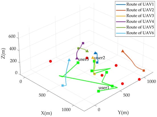
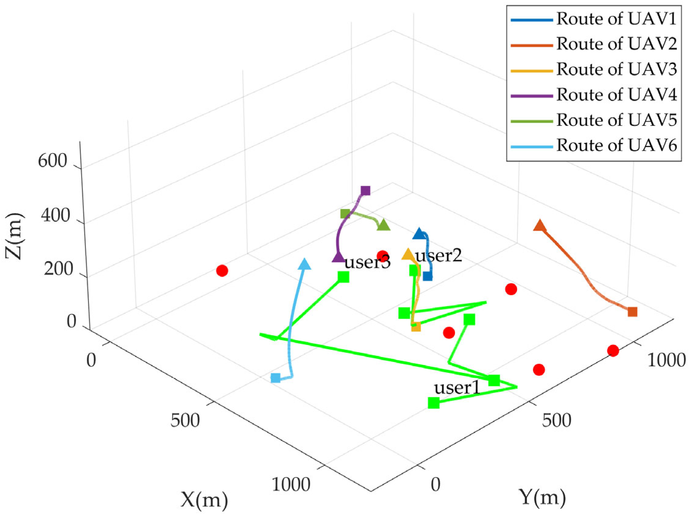
Figure 7 presents a 3D visualization of the UAV swarm trajectories throughout the 600 s simulation, overlaid with the ground anchors (red circles), initial UAV positions (colored triangles), and the complete user trajectories (green blocks to show the start and destination). The UAVs can be seen dynamically repositioning in response to each user velocity transition, spreading out and adjusting altitude to maintain favorable geometric diversity.

Figure 7. Autonomous planned route of UAV swarm in the dynamic scenario. Red circles: ground anchors; colored triangles and squares: initial UAV positions and final UAV positions in the mission; green squares: dynamic users.

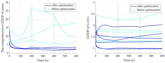
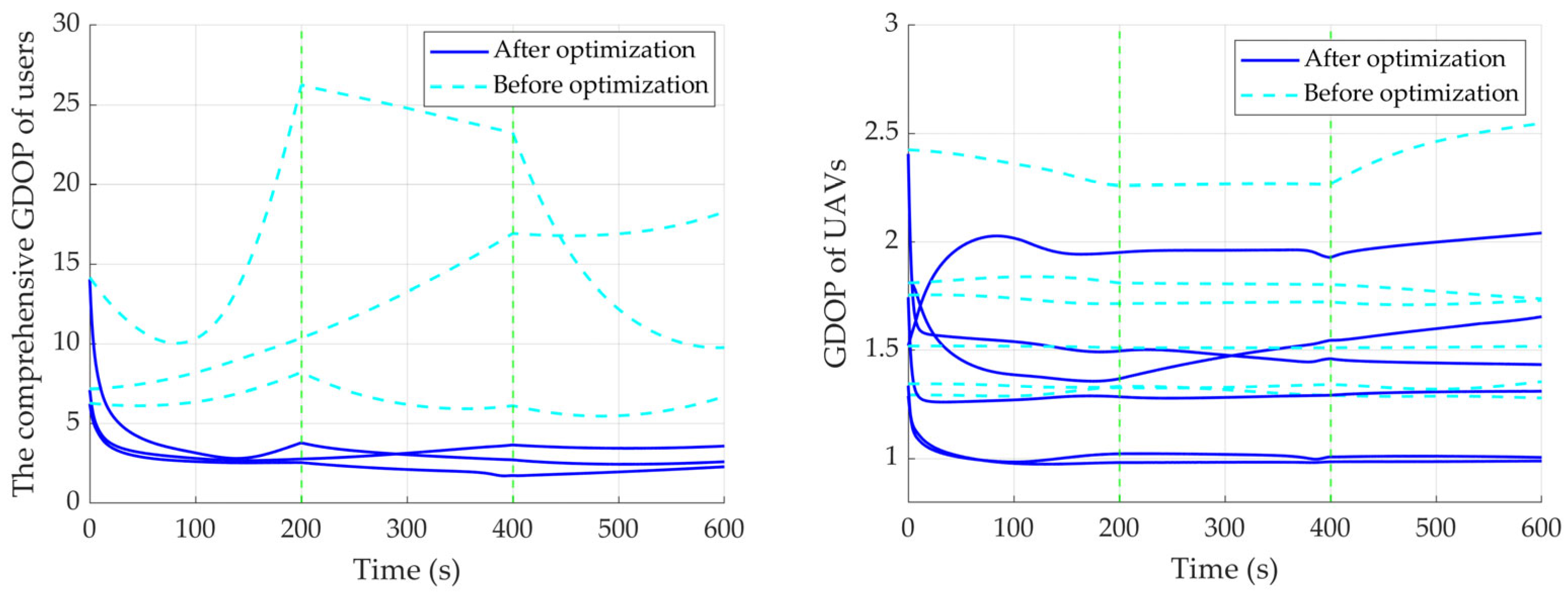
Figure 8 compares the time evolution of the average in users’ comprehensive GDOP $G_U$ (solid blue line) with that of a non-adaptive baseline where the UAVs remain fixed at their initial positions (dashed light blue line). Several key observations emerge: (1) The proposed algorithm achieves rapid convergence, reducing the $G_U$ to values consistently below 4, often approaching 2.0–2.5 after user velocity changes. (2) At the velocity transition points ($t=200 \mathrm{s}$ and $t=400 \mathrm{s}$), the $G_U$ and UAVs’ GDOP $G_W$ experience a brief spike in both cases due to sudden geometry degradation; however, the adaptive UAV swarm remains stable, while the static baseline shows persistent high GDOP. (3) Across the entire 600 s, the adaptive method yields a significantly lower mean $G_U$ for 2.92 compared to the static baseline of 12.92, achieved a 76.1% improvement. It is worth noting that the inter-user balance (lower variance among the three users), and greater temporal stability (smoother curves with fewer fluctuations) are also enhanced.

Figure 8. Evolution of the comprehensive GDOP of users and the GDOP of UAVs over time in the dynamic scenario.

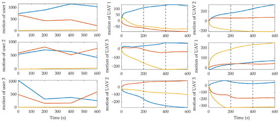
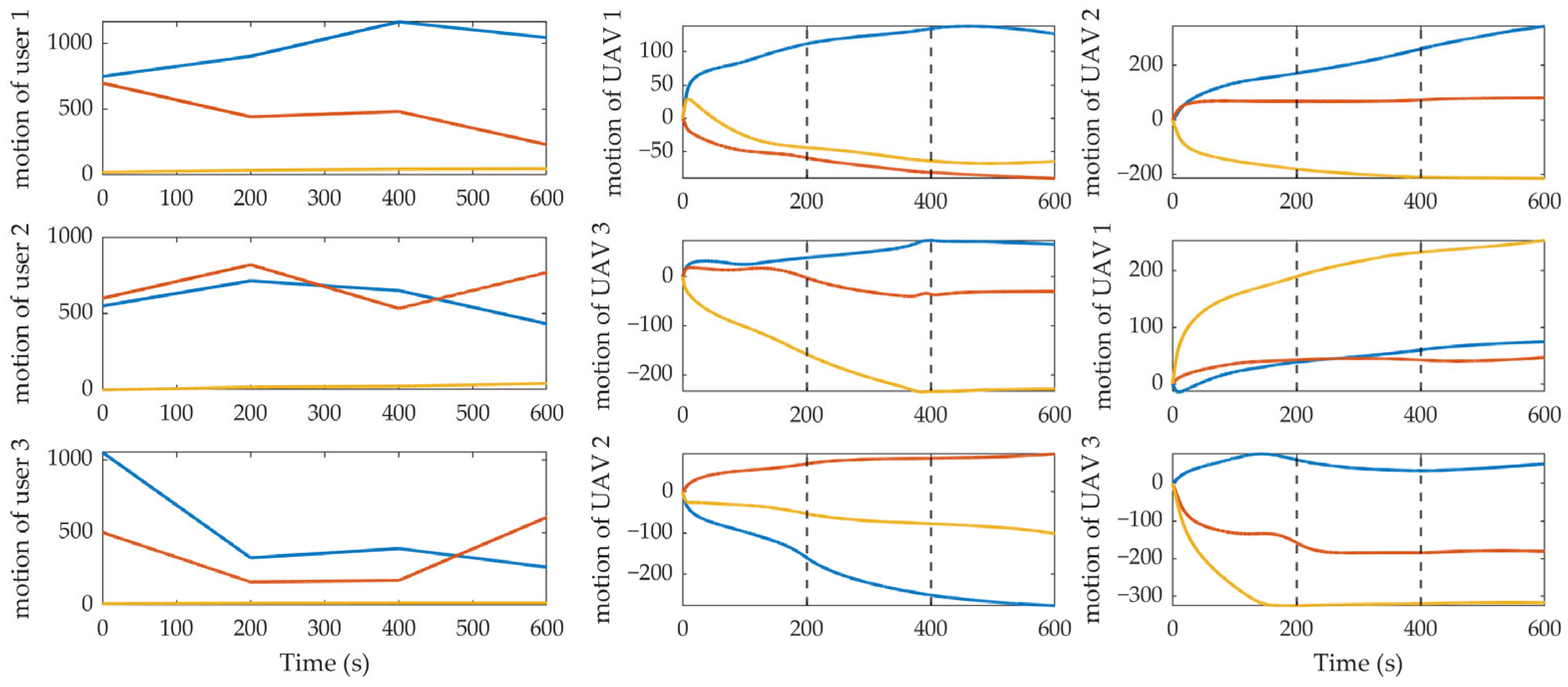
Figure 9 further illustrates the x (blue), y (red), and z (yellow) position histories of the UAV swarm and users over time. The UAV routes’ data have had the initial coordinates subtracted to exhibit clear, coordinated adjustments at $t=200 \mathrm{s}$ and $t=400 \mathrm{s}$, with noticeable velocity changes in response to the user motion discontinuities. These plots visually confirm the swarm’s self-adaptive capability: when user states change abruptly, the attractive potential gradient strengthens, prompting immediate repositioning to restore geometric quality.

Figure 9. Time histories of users and UAVs positions along x, y, z axis.

The results in this dynamic scenario demonstrate that the proposed framework not only converges effectively under time-varying conditions but also exhibits strong robustness and adaptability to sudden user state changes. Compared to the static baseline, the algorithm substantially improves user positioning accuracy, inter-user equity, and temporal consistency, validating its suitability for real-world air–terrestrial cooperative navigation applications involving heterogeneous and mobile users.

While the simulation results in static and dynamic scenarios demonstrate strong convergence and adaptability of the proposed APF framework, it is important to acknowledge the inherent limitations of classical Artificial Potential Field methods, including local minima, oscillations in narrow passages, and target unreachability. In our specific application—real-time geometric configuration optimization for UAV swarms serving dynamic ground users in GNSS-denied regional navigation—these defects manifest less severely than in traditional obstacle-dense path planning tasks. First, the primary objective is continuous, reactive minimization of user GDOP rather than convergence to a single global optimum position; thus, even if a UAV enters a local minimum, the resulting geometry often remains acceptable due to the relatively flat and forgiving nature of GDOP landscapes in multi-UAV configurations. Second, the operating environment is relatively open (airspace with sparse ground anchors), significantly reducing the probability of narrow-channel oscillations. Third, the repulsive potentials designed for minimum altitude and inter-UAV separation naturally promote swarm diversity, which helps mitigate trap situations by preventing excessive clustering. These characteristics make the classical APF particularly suitable for our lightweight, onboard-real-time requirements, where computational simplicity outweighs the need for guaranteed global optimality. Future work may incorporate adaptive gain tuning or random perturbations to further enhance robustness in more constrained environments.

4.3. Analysis of Computational Complexity

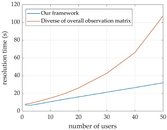
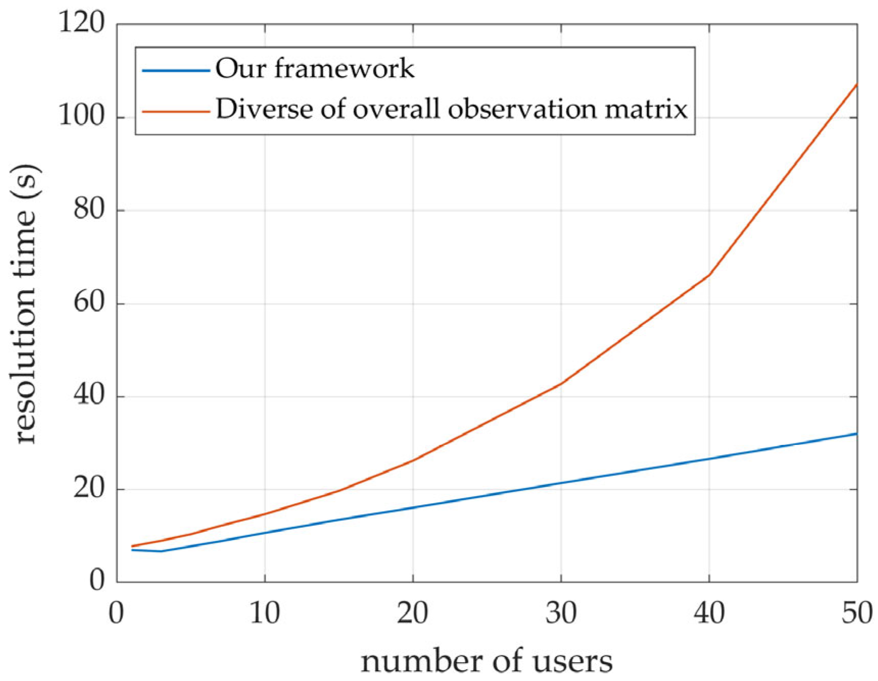
To verify the practical effectiveness of the proposed Schur-complement-based geometric evaluation model in reducing computational complexity, this section provides a quantitative comparative analysis. The simulations were performed on a computing platform equipped with an AMD Ryzen 7 5800 H CPU and 32 GB RAM. To simulate diverse air–terrestrial cooperative navigation scenarios ranging from sparse to dense, the number of UAVs was fixed at $J=6$, while the number of users ($K$) was varied from 3 to 50. Each experiment was executed 1000 times to obtain the average processing time and eliminate random fluctuations. The results are shown in Figure 10.

Figure 10. Time complexity simulations results.

As illustrated in the figure, within the range of 3 to 50 users, computational complexity is reduced from an exponential growth trend to an approximately linear progression following matrix decomposition. Specifically, at a scale of 30 users, the processing time is effectively halved, and it further decreases to approximately one-third of the baseline when the user count reaches 50. This clearly demonstrates the efficacy of our proposed method, particularly its superior scalability in scenarios involving large-scale user populations.

5. Conclusions

This paper proposed a lightweight, APF-based framework for autonomous UAV swarm route planning in dynamic air–terrestrial cooperative navigation scenarios operating in GNSS-denied environments. By integrating a Schur-complement-based geometric evaluation metric directly into the attractive potential, the method enables the UAV swarm to continuously optimize its configuration in real time so as to minimize user positioning errors while satisfying operational constraints such as minimum altitude and inter-UAV separation.

The core innovation lies in decomposing the full system precision covariance matrix via the Schur complement, yielding a scalar, differentiable user-equivalent GDOP function that faithfully captures end-to-end geometric quality. This metric is then used to construct the attractive potential, with virtual forces derived via a computationally efficient finite-difference approximation, ensuring onboard real-time feasibility even on resource-constrained UAV platforms.

Extensive simulations validated the framework across static and dynamic scenarios. In the static case, the algorithm drove the UAV swarm from poor initial geometries to near-optimal configurations, reducing the average user GDOP from approximately 10 to below 4 within 150 s and maintaining stable convergence. In the dynamic scenario involving piecewise constant-velocity user motion over 600 s, the swarm exhibited rapid adaptive navigation at each velocity transition point. Compared to the baseline of fixed UAV positions, the proposed method achieved substantial performance gains: the mean user comprehensive GDOP was reduced by 76.1% on average. Moreover, the algorithm significantly enhanced inter-user balance and temporal stability, demonstrating its effectiveness in handling heterogeneous and mobile user demands.

These results confirm that the framework successfully bridges high-level navigation performance optimization with low-level motion control, offering a practical solution for real-time UAV swarm coordination in GNSS-denied air–terrestrial positioning networks.

References

- Wang, J.; Xiao, Y.; Li, T.; Chen, C.P. A Jamming Aware Artificial Potential Field Method to Counter GPS Jamming for Unmanned Surface Ship Path Planning. IEEE Syst. J. 2023, 17, 4555–4566. [Google Scholar] [CrossRef] [Scilit]
- Morton, Y.J.; van Diggelen, F.; Spilker, J.J., Jr.; Parkinson, B.W.; Lo, S.; Gao, G. Position, Navigation, and Timing Technologies in the 21st Century; Wiley: Hoboken, NJ, USA, 2021; Volume 1. [Google Scholar]
- Budiyono, A. Principles of GNSS, Inertial, and Multisensor Integrated Navigation Systems—Second Edition Paul D. Groves Artech House, 2013, 776 pp ISBN-13: 978-1-60807-005-3. J. Navig. 2014, 67, 191–192. [Google Scholar]
- Njima, W.; Bazzi, A.; Chafii, M. DNN-Based Indoor Localization under Limited Dataset Using GANs and Semi-Supervised Learning. IEEE Access 2022, 10, 69896–69909. [Google Scholar] [CrossRef] [Scilit]
- Dou, Z.; Yao, Z.; Lu, M. Distributed Radio Local Positioning System Spatial Reference Autonomous Establishment Technology. Acta Electron. Sin. 2022, 50, 841–848. [Google Scholar]
- Zhang, X.; Chen, J.; Xin, B.; Peng, Z. A Memetic Algorithm for Path Planning of Curvature-Constrained UAVs Performing Surveillance of Multiple Ground Targets. Chin. J. Aeronaut. 2014, 27, 622–633. [Google Scholar] [CrossRef] [Scilit]
- Kim, E. A Coverage Analysis Methodology for APNT Pseudolite Ground Network. In Proceedings of the 24th International Technical Meeting of the Satellite Division of the Institute of Navigation (ION GNSS 2011), Portland, OR, USA, 20–23 September 2011; pp. 495–507. [Google Scholar]
- Khalife, J.; Kassas, Z.M. Opportunistic UAV Navigation with Carrier Phase Measurements from Asynchronous Cellular Signals. IEEE Trans. Aerosp. Electron. Syst. 2019, 56, 3285–3301. [Google Scholar] [CrossRef] [Scilit]
- Yang, X.; Liu, W.; Ye, X.; Li, X.; Wei, S.; Wang, F. A Geometry-Based Method for the Rapid Deployment of a UAV Pseudolite Navigation System in a Target Area. J. Geod. 2023, 97, 90. [Google Scholar] [CrossRef] [Scilit]
- Tang, X.; Chen, F.; Wang, F.; Jia, Z. Disaster-Resilient Emergency Communication with Intelligent Air–Ground Cooperation. IEEE Internet Things J. 2024, 11, 5331–5346. [Google Scholar] [CrossRef] [Scilit]
- Ding, T.; Liu, L.; Yan, Z.; Lu, X.; Hu, J. Federated Reinforcement Learning for Intelligent Route Planning in Aerial-Terrestrial Network. IEEE Internet Things J. 2024, 12, 43909–43921. [Google Scholar] [CrossRef] [Scilit]
- Liu, Q.; Liu, R.; Xu, C. Prospective UAV-Assisted Positioning Architecture and Technologies for 6G Network Edge. IEEE Netw. 2024, 39, 61–68. [Google Scholar] [CrossRef] [Scilit]
- Verdone, R.; Mignardi, S. Joint Aerial-Terrestrial Resource Management in UAV-Aided Mobile Radio Networks. IEEE Netw. 2018, 32, 70–75. [Google Scholar] [CrossRef] [Scilit]
- Han, S.; Gong, Z.; Meng, W.; Li, C.; Gu, X. Future Alternative Positioning, Navigation, and Timing Techniques: A Survey. IEEE Wirel. Commun. 2016, 23, 154–160. [Google Scholar] [CrossRef] [Scilit]
- Cheng, X.; Han, G.; Peng, J.; Jiang, J.; He, Y.; Zhu, W.; Shu, F.; Wang, J. An ADMM-Based Geometric Configuration Optimization in RSSD-Based Source Localization by UAVs with Spread Angle Constraint. IEEE Trans. Veh. Technol. 2024, 74, 5504–5516. [Google Scholar] [CrossRef] [Scilit]
- Wu, Z.; Yao, Z.; Lu, M. Waypoint Selection for Unmanned Aerial Vehicle-Aided Calibration in Wireless Positioning Networks. IET Radar Sonar Navig. 2023, 17, 1088–1099. [Google Scholar] [CrossRef] [Scilit]
- Li, H.; Sun, H.; Zhou, R.; Zhang, H. Hybrid TDOA/FDOA and Track Optimization of UAV Swarm Based on A-Optimality. J. Syst. Eng. Electron. 2023, 34, 149–159. [Google Scholar] [CrossRef] [Scilit]
- Zhou, R.; Sun, H.; Li, H.; Luo, W. TDOA and Track Optimization of UAV Swarm Based on D-Optimality. J. Syst. Eng. Electron. 2020, 31, 1140–1151. [Google Scholar] [CrossRef] [Scilit]
- Chen, M.; Xiong, Z.; Liu, J.; Wang, R.; Xiong, J. Cooperative Navigation of Unmanned Aerial Vehicle Swarm Based on Cooperative Dilution of Precision. Int. J. Adv. Robot. Syst. 2020, 17, 1729881420932717. [Google Scholar] [CrossRef] [Scilit]
- Deb, K.; Jain, H. An Evolutionary Many-Objective Optimization Algorithm Using Reference-Point-Based Nondominated Sorting Approach, Part I: Solving Problems with Box Constraints. IEEE Trans. Evol. Comput. 2013, 18, 577–601. [Google Scholar] [CrossRef] [Scilit]
- Huang, J.; Tao, Z.; He, J. Deep Reinforcement Learning Method of UAV Behavior Planning for Optimizing Geometric Dilution Precision Distribution. In 2022 5th International Conference on Advanced Electronic Materials, Computers and Software Engineering (AEMCSE); IEEE: New York, NY, USA, 2022; pp. 276–280. [Google Scholar]
- Ebrahimi, D.; Sharafeddine, S.; Ho, P.-H.; Assi, C. Autonomous UAV Trajectory for Localizing Ground Objects: A Reinforcement Learning Approach. IEEE Trans. Mob. Comput. 2020, 20, 1312–1324. [Google Scholar] [CrossRef] [Scilit]
- Khatib, O. Real-Time Obstacle Avoidance for Manipulators and Mobile Robots. Int. J. Robot. Res. 1986, 5, 90–98. [Google Scholar] [CrossRef] [Scilit]
- Bu, Y.; Yan, Y.; Yang, Y. Advancement Challenges in UAV Swarm Formation Control: A Comprehensive Review. Drones 2024, 8, 320. [Google Scholar] [CrossRef] [Scilit]
- Kozlov, E.; Muslimov, T. Artificial Potential Field Method for Path and Trajectory Planning of Unmanned Aerial Vehicles: A Review. Unmanned Syst. 2025. [Google Scholar] [CrossRef] [Scilit]
- Koren, Y.; Borenstein, J. Potential Field Methods and Their Inherent Limitations for Mobile Robot Navigation. In Proceedings of the 1991 IEEE International Conference on Robotics and Automation (ICRA), Sacramento, CA, USA, 9–11 April 1991; Volume 2, pp. 1398–1404. [Google Scholar]
- Hao, G.; Lv, Q.; Huang, Z.; Zhao, H.; Chen, W. UAV Path Planning Based on Improved Artificial Potential Field Method. Aerospace 2023, 10, 562. [Google Scholar] [CrossRef] [Scilit]
- Klančar, G.; Zdešar, A.; Krishnan, M. Robot Navigation Based on Potential Field and Gradient Obtained by Bilinear Interpolation and a Grid-Based Search. Sensors 2022, 22, 3295. [Google Scholar] [CrossRef] [Scilit] [PubMed]
- Bounini, F.; Gingras, D.; Pollart, H.; Gruyer, D. Modified Artificial Potential Field Method for Online Path Planning Applications. In 2017 IEEE Intelligent Vehicles Symposium (IV); IEEE: New York, NY, USA, 2017; pp. 180–185. [Google Scholar]
- Shin, Y.; Kim, E. Hybrid Path Planning Using Positioning Risk and Artificial Potential Fields. Aerosp. Sci. Technol. 2021, 112, 106640. [Google Scholar] [CrossRef] [Scilit]
Disclaimer/Publisher’s Note: The statements, opinions and data contained in all publications are solely those of the individual author(s) and contributor(s) and not of MDPI and/or the editor(s). MDPI and/or the editor(s) disclaim responsibility for any injury to people or property resulting from any ideas, methods, instructions or products referred to in the content. |
© 2026 by the authors. Licensee MDPI, Basel, Switzerland. This article is an open access article distributed under the terms and conditions of the Creative Commons Attribution (CC BY) license.