Modeling and Trajectory Tracking Control for Double- Steering Wheeled Climbing Robot Based on Adaptive Dynamic Programming

Abstract

A model and tracking control method for a double-steering wheeled climbing robot (DSWCR) are presented in this article. The dynamic model of the DSWCR system is established using the Lagrange equation, considering the effects of slipping, variations in gravity and the friction coefficient, and wall/wheel interaction forces. During wall motion, the DSWCR is subject to uncertainties introduced from both the state and model. To address the tracking problem of the DSWCR under state and model uncertainties, an adaptive dynamic programming (ADP) controller based on zero-sum theory is proposed. The stability of the DSWCR tracking system and the convergence of the weights in a neural network are demonstrated. Finally, simulations and a prototype experiment are conducted to verify the optimality and robustness of the proposed control method.

1. Introduction

Regular inspection of wall defects is an essential part of the maintenance tasks of large steel structures. The traditional methods to reach the wall surface are scaffolding, an elevated work platform or manual climbing, which have potential safety hazards and high labor costs. In order to improve operational efficiency and eliminate the safety hazards, the introduction of a wall-climbing robot equipped with inspection sensors has become a viable method. The wall-climbing robot can reach the area to be inspected and accurately detect wall defects.

The current wall-climbing robots can be divided into different types based on their move mode [1,2,3,4], such as wheeled, caterpillar and legged. Additionally, they can be divided according to the method of adhesion, such as permanent magnetic, electromagnetic, and vacuum suction. Among the various combinations of move modes and adhesion methods, the permanent magnetic wheeled climbing robot has been widely employed in wall-climbing robot structures due to its advantages of simplicity, continuous motion, and ease of manufacturing and maintenance [5].

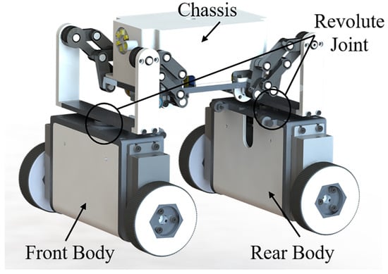
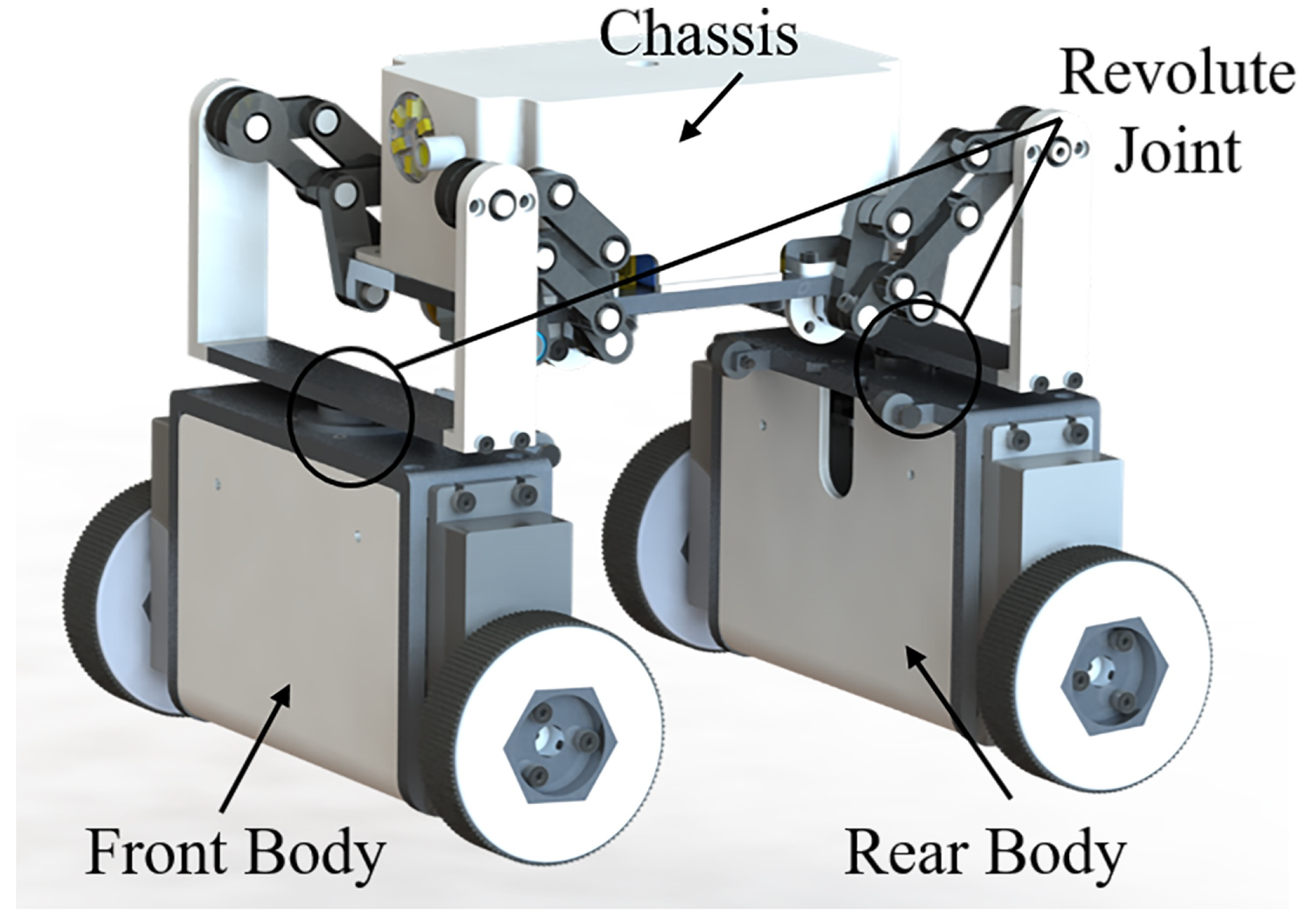
Considering the stability and the maneuverability during wall surface tasks, we have proposed a double-steering wheeled climbing robot (DSWCR). As shown in Figure 1, the robot consists of a front body, a rear body, and a chassis. The front and rear bodies are equipped with a pair of driving magnetic wheels, and steering can be achieved by adjusting the speed difference between the wheels on both sides. The front and rear body are connected to the chassis through a revolute joint. Compared to the traditional four-wheel skid-steering climbing robot (SSCR), the DSWCR incorporates an additional degree of steering freedom through its dual-steering mechanism. In SSCRs, turning heavily relies on differential wheel speeds to overcome immense lateral friction, which often leads to severe energy loss and unpredictable slip. Conversely, the structural design of the DSWCR effectively reduces the lateral slip forces required during turning maneuvers. Consequently, the DSWCR not only lowers energy consumption but also significantly enhances steering stability, maneuverability, and control precision when tracking complex trajectories on wall surfaces [6,7].

Figure 1. The structure of the DSWCR system.

In practical applications, it is necessary for a wall-climbing robot to track target trajectories, which imposes high requirements on the robot’s tracking ability. To achieve the precision tracking of the DSWCR, it is crucial to design a controller that takes into account the robot’s structural characteristics and working conditions. The DSWCR is a control system with underactuated, strong coupling, and nonlinear characteristics. The control inputs for the DSWCR include the velocity and angular velocity of the front and rear body. The system’s degrees of freedom encompass displacements in the XY direction, as well as the yaw angle of the front and rear body and the chassis. Due to having fewer control inputs than the system’s degrees of freedom, the DSWCR is an underactuated system. Furthermore, the structural design of the DSWCR leads to a coupling relationship between the velocity and angular velocity of the front and rear body, where changes in individual input variables can impact the overall system state.

When modeling and designing a controller for the DSWCR system, it is necessary to consider the uncertainties. Uncertainties can be divided into state uncertainty and model uncertainties. State uncertainty is generated by the sensor noise and measurement errors and introduced via measurement. Model uncertainties include the effects of uncertain wheel/wall interaction forces and slipping on the robot’s motion. The interaction forces vary due to factors such as gravity, the rolling friction coefficient, magnetic force, and wall inclination, thereby causing different effects on the motion. When the robot experiences slip, the wheels exhibit varying degrees of lateral and longitudinal slipping, resulting in errors in trajectory tracking. Both state and model uncertainties pose challenges to the tracking control of the DSWCR system. The novelty of this study lies in applying an adaptive dynamic programming (ADP) zero-sum game controller to the underactuated DSWCR. This approach effectively handles both state and model uncertainties. Furthermore, unlike existing simplified models, our dynamic model explicitly includes wheel slip and complex wheel/wall interaction forces. As a result, the robot achieves optimal and robust trajectory tracking in uncertain wall-climbing environments.

To actualize these novel concepts, this paper makes the following concrete contributions: (1) For the underactuated and strongly coupled DSWCR system, a rigorous dynamic model is established using the Lagrange equation. This model accurately captures the wheel/wall interaction forces and wheel slip dynamics. (2) An adaptive dynamic programming controller based on zero-sum game theory is designed. This controller achieves optimal trajectory tracking while maintaining robustness against both state and model uncertainties. (3) Based on Lyapunov theory, the overall stability of the DSWCR tracking system and the convergence of the weights in the critic network are mathematically proven.

2. Related Works

2.1. Modeling of Wheeled Climbing Robots

In recent years, several research works have focused on the modeling of wheeled wall-climbing robots [7,8,9,10]. Dian et al. [11] and Lyu Guizhi et al. [12] considered the influence of gravity and the rolling friction coefficient on the wheel/wall interaction forces in their model of a four-wheel skid-steering climbing robot (SSCR). Santos H. B. et al. [13] further incorporated the effects of wall inclination and robot pose on the wheel/wall interaction forces. A Chokshi et al. [14] and D. L. Tang et al. [15] considered the impact of both lateral and longitudinal friction forces on wheel slip. However, the above studies mainly focused on the SSCR structure, without consideration of both complex wheel/wall interactions and slip. Therefore, part of the work in this paper aims to model the DSWCR system by integrating the effects of wheel/wall interaction forces and slip.

2.2. Trajectory Tracking Control Methods

Although advanced trajectory tracking and predictive optimization strategies have been extensively developed for conventional mobile robots and unmanned vehicles [16,17], wheeled wall-climbing robots face unique and severe challenges induced by complex wheel/wall interactions and instantaneous slip. Currently, research on trajectory tracking for wheeled wall-climbing robots mainly focuses on traditional control methods such as PID [18,19], MPC [13,20] and backstepping [21,22]. While these controllers are relatively simple, they tend to be ineffective when dealing with complex systems and uncertainties. In recent years, various intelligent control algorithms have been proposed in the fields of ground mobile robots and robotic arm control, such as adaptive control [23,24,25,26], neural network control [27,28] and fuzzy control [29,30]. These methods exhibit strong adaptive capabilities and do not rely on a precise mathematical model of the system. However, their application in wheeled wall-climbing robots is limited, especially under complex wall conditions where slow adaptive parameter adjustment becomes an issue [31]. To address this problem, some researchers have introduced adaptive dynamic programming (ADP) into the tracking of wheeled climbing robots. This approach not only resolves the issue of slow parameter adjustment but also shows optimal control performance. ADP integrates the advantages of reinforcement learning, dynamic programming and neural networks, enabling adaptive control with advantageous parameter adaptation in optimal control of complex systems. It has been widely applied in the field of trajectory tracking control. Dian et al. [11] established the dynamic model of a four-wheel SSCR and achieved precise trajectory tracking control using an improved DHP algorithm and a reinforcement learning framework. In the DHP algorithm, they introduced a genetic algorithm to optimize the neural network, thereby enhancing the adaptability of the parameters. Subsequently, Fang et al. [31] further developed an online robust tracking controller based on ADP. They simplified the critic and action networks to achieve better tracking for a four-wheel SSCR. The object of the above research works is a four-wheel SSCR, which belongs to a fully actuated system. They primarily focus on the uncertainties caused by errors in modeling and overlook the impacts of state uncertainties and wheel slip.

3. Modeling of DSWCR

3.1. Structure of DSWCR

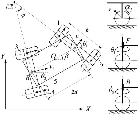
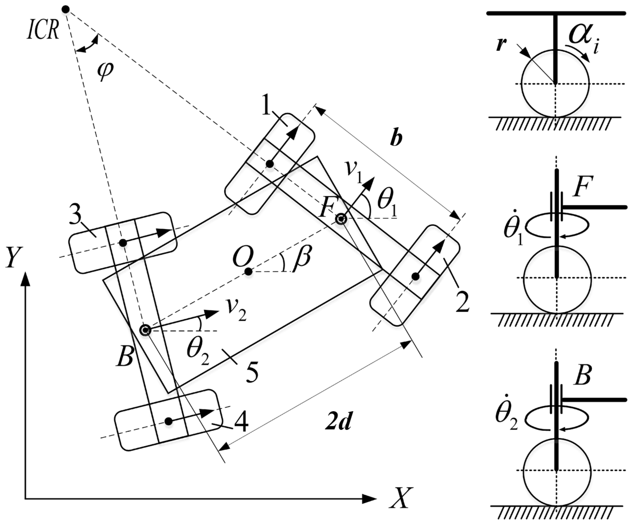
The schematic diagram in Figure 2 depicts the nonholonomic DSWCR system. The mass center of the robot is located at point O, while the front and rear body are represented by points F and B, respectively. The variable definitions of the robot are provided in Table 1.

Figure 2. Schematic diagram of DSWCR nonholonomic system.

Table 1. Definition of DSWCR system parameters.

Notation	Definition
b	Distance between parallel wheels
$2d$	Distance between points F and B
$x_1,y_1$	The position of point F in X-Y coordinates
$x_2,y_2$	The position of point B in X-Y coordinates
${\theta }_1$	Yaw angle of the front body
${\theta }_2$	Yaw angle of the rear body
${\alpha }_1,{\alpha }_2,{\alpha }_3,{\alpha }_4$	Rotation angels of the magnetic wheel
$M_w$	Mass of the magnetic wheel
$M_f$	Mass of the front body
$M_r$	Mass of the rear body
$M_p$	Mass of the chassis
$I_w$	Moment of inertia of the magnetic wheel along the wheel axis direction
$I_{wz}$	Moment of inertia of the wheel about the Z-axis through the center of the wheel
$I_f$	Moment of inertia of the front body about the Z-axis through the center point F
$I_b$	Moment of inertia of the rear body about the Z-axis through the center point B
$I_c$	Moment of inertia of the framework about the Z-axis through the center point C
r	Radius of the magnetic wheel
$\beta$	Yaw angle of the chassis
${\tau }_1,{\tau }_2$	The driving torques of wheel 1 and wheel 2
${\tau }_3,{\tau }_4$	The driving torques of wheel 3 and wheel 4

3.2. Kinematic Model of DSWCR

In this section, an analysis of the kinematic model of the DSWCR is conducted. In the inertial coordinate system $\{X,Y\}$, the generalized coordinate vector q of the DSWCR is expressed as follows:

$$q={[x_1,y_1,{\theta }_1,{\theta }_2,\beta ,{\alpha }_1,{\alpha }_2,{\alpha }_3,{\alpha }_4]}^T$$

(1)

When the robot moves on a wall surface, it is susceptible to slipping due to the influence of gravity. It is necessary to model the uncertainties caused by slipping. Referring to study [32], the constraint equations considering slip and nonholonomic constraints can be written as follows:

$$\begin{array}{c}\left\{\begin{array}{c}{\dot{x}}_{1}cos{\theta }_1+{\dot{y}}_{1}sin{\theta }_1-b{\dot{\theta }}_1=r({\dot{\alpha }}_1-{\dot{\xi }}_{l1})\\ {\dot{x}}_{1}cos{\theta }_1+{\dot{y}}_{1}sin{\theta }_1+b{\dot{\theta }}_1=r({\dot{\alpha }}_2-{\dot{\xi }}_{r1})\\ -{\dot{x}}_{1}sin{\theta }_1+{\dot{y}}_{1}cos{\theta }_1={\dot{\eta }}_1\end{array}\right.\hfill \\ \left\{\begin{array}{c}{\dot{x}}_{2}cos{\theta }_2+{\dot{y}}_{2}sin{\theta }_2-b{\dot{\theta }}_2=r({\dot{\alpha }}_3-{\dot{\xi }}_{l2})\\ {\dot{x}}_{2}cos{\theta }_2+{\dot{y}}_{2}sin{\theta }_2+b{\dot{\theta }}_2=r({\dot{\alpha }}_4-{\dot{\xi }}_{r2})\\ -{\dot{x}}_{2}sin{\theta }_2+{\dot{y}}_{2}cos{\theta }_2={\dot{\eta }}_2\end{array}\right.\hfill \end{array}$$

(2)

where ${\xi }_{li}$ and ${\xi }_{ri}$ represent the longitudinal slip displacement of the left and right magnetic wheels, respectively; ${\eta }_i$ represents the lateral slip displacement; and $i=\{1,2\}$ represents the front and rear car bodies respectively. The slip terms ${\xi }_{l1},{\xi }_{r1},{\xi }_{l2},{\xi }_{r2},{\eta }_1,{\eta }_2$ and their first and second derivatives are bounded. Due to the symmetric distribution of the magnetic wheels, there is no relative motion in the lateral direction, so their lateral slip displacements are the same.

By geometric relationships, the constraint Equation (3) can be obtained. Taking the time derivatives of both sides of the equation, we have

$$\left\{\begin{array}{c}{x}_1=x_2+2dcos\beta \\ y_1=y_2+2dsin\beta \end{array}\right.\left\{\begin{array}{c}{\dot{x}}_2={\dot{x}}_1+2d\dot{\beta }sin\beta \\ {\dot{y}}_2={\dot{y}}_1-2d\dot{\beta }cos\beta \end{array}\right.$$

(3)

The instantaneous velocity of the front body is $v_1$, while that of the rear body is $v_2$. $v_1$ and $v_2$ satisfy the following relationship:

$$\left\{\begin{array}{c}{v}_1={\dot{x}}_{1}cos{\theta }_1+{\dot{y}}_{1}sin{\theta }_1\\ v_2={\dot{x}}_{2}cos{\theta }_2+{\dot{y}}_{2}sin{\theta }_2\end{array}\right.$$

(4)

Substituting Equation (4) into Equation (3) and eliminating d, we obtain the constraint between $v_1$ and $v_2$:

$$v_{2}cos(\beta -{\theta }_2)=v_{1}cos(\beta -{\theta }_1)$$

(5)

Substituting Equation (5) into Equation (3), we can obtain the yaw angular acceleration of the chassis $\dot{\beta }$:

$$\dot{\beta }={\displaystyle \frac{sin({\theta }_1-{\theta }_2)}{2dcos(\beta -{\theta }_2)}}{v}_1$$

(6)

Defining the kinematic equation as $F(q)\dot{q}=0$, we can obtain the kinematic matrix $F(q)$ from Equation (3) to Equation (5):

$$F(q)=\left[\begin{array}{ccccccccc}cos{\theta }_1& sin{\theta }_1& -b& 0& 0& -r& 0& 0& 0\\ cos{\theta }_1& sin{\theta }_1& b& 0& 0& 0& -r& 0& 0\\ -sin{\theta }_1& cos{\theta }_1& 0& 0& 0& 0& 0& 0& 0\\ cos{\theta }_2& sin{\theta }_2& 0& -b& 2dsin(\beta -{\theta }_2)& 0& 0& -r& 0\\ cos{\theta }_2& sin{\theta }_2& 0& b& 2dsin(\beta -{\theta }_2)& 0& 0& 0& -r\\ -sin{\theta }_2& cos{\theta }_2& 0& 0& -2dcos(\beta -{\theta }_2)& 0& 0& 0& 0\end{array}\right]$$

(7)

$F(q)\in {\Re }^{m\times n}$ represents the kinematic matrix of the DSWCR. Define $S(q)\in {\Re }^{n\times (n-m)}$ as a full-rank matrix, which is also the nullspace matrix of $F(q)$, satisfying $F(q)S(q)=0$. We can obtain another form of the kinematic model as $\dot{q}=S(q)x$:

$$S(q)={\left[\begin{array}{ccccccccc}cos{\theta }_1& sin{\theta }_1& 0& 0& {\displaystyle \frac{sin({\theta }_1-{\theta }_2)}{2dcos(\beta -{\theta }_2)}}& {\displaystyle \frac{1}{r}}& {\displaystyle \frac{1}{r}}& {\displaystyle \frac{cos(\beta -{\theta }_1)}{cos(\beta -{\theta }_2)r}}& {\displaystyle \frac{cos(\beta -{\theta }_1)}{cos(\beta -{\theta }_2)r}}\\ 0& 0& 1& 0& 0& -{\displaystyle \frac{b}{r}}& {\displaystyle \frac{b}{r}}& 0& 0\\ 0& 0& 0& 1& 0& 0& 0& -{\displaystyle \frac{b}{r}}& {\displaystyle \frac{b}{r}}\end{array}\right]}^T$$

(8)

where $x\in {\Re }^{(n-m)\times 1}={(v_1,{\dot{\theta }}_1,{\dot{\theta }}_2)}^T$. Considering the influence of slip, referring to study [33], the kinematic model can be rewritten as

$$\dot{q}=S(q)(x(t)-\dot{\xi }(t))+\psi (q,\dot{\eta })$$

(9)

where $\psi (q,\dot{\eta })={[-{\dot{\eta }}_{1}sin{\theta }_1,{\dot{\eta }}_{1}cos{\theta }_1,0,0,0,{\displaystyle \frac{{\dot{\eta }}_1}{r}},{\displaystyle \frac{{\dot{\eta }}_1}{r}},{\displaystyle \frac{{\dot{\eta }}_2}{r}},{\displaystyle \frac{{\dot{\eta }}_2}{r}}]}^T$, $\dot{\xi }(t)={[{\dot{\xi }}_v,{\dot{\xi }}_{\theta 1},{\dot{\xi }}_{\theta 2}]}^T, {\dot{\xi }}_v={\displaystyle \frac{{\dot{\xi }}_{l1}+{\dot{\xi }}_{r1}}{2}}$, ${\dot{\xi }}_{\theta 1}={\displaystyle \frac{{\dot{\xi }}_{r1}-{\dot{\xi }}_{l1}}{2b}}, {\dot{\xi }}_{\theta 2}={\displaystyle \frac{{\dot{\xi }}_{r2}-{\dot{\xi }}_{l2}}{2b}}$.

3.3. Dynamic Model of DSWCR

In this section, the Lagrange equation with a multiplier is used to establish the dynamic model of the DSWCR:

$${\displaystyle \frac{d}{dt}}\left({\displaystyle \frac{\partial L}{\partial \dot{q}}}\right)-{\displaystyle \frac{\partial L}{\partial q}}=Q+F^T(q)\lambda$$

(10)

where $L=E-V$, E represents the kinetic energy, V represents the potential energy, Q represents the generalized forces, and $\lambda$ is the Lagrange multiplier.

The kinetic energy of the DSWCR is divided into three parts: the kinetic energy of the front body $E_1$, the rear body $E_2$, and the chassis $E_3$. The expressions of $E_1$ and $E_2$ are as follows:

$$\begin{array}{c}\hfill \left\{\begin{array}{cc}{E}_1\hfill & ={\displaystyle \frac{1}{2}}{M}_w({\dot{\alpha }}_1^2+{\dot{\alpha }}_2^2)r^2+{\displaystyle \frac{1}{2}}{I}_w({\dot{\alpha }}_1^2+{\dot{\alpha }}_2^2)+I_{wz}{\dot{\theta }}_1^2+{\displaystyle \frac{1}{2}}{M}_f({\dot{x}}_1^2+{\dot{y}}_1^2)+{\displaystyle \frac{1}{2}}{I}_f{\dot{\theta }}_1^2\hfill \\ E_2\hfill & ={\displaystyle \frac{1}{2}}{M}_w({\dot{\alpha }}_3^2+{\dot{\alpha }}_4^2)r^2+{\displaystyle \frac{1}{2}}{I}_w({\dot{\alpha }}_3^2+{\dot{\alpha }}_4^2)+I_{wz}{\dot{\theta }}_2^2+{\displaystyle \frac{1}{2}}{M}_r({\dot{x}}_1^2+{\dot{y}}_1^2){\displaystyle \frac{{cos}^2(\beta -{\theta }_1)}{{cos}^2(\beta -{\theta }_2)}}\hfill \\ & +{\displaystyle \frac{1}{2}}{I}_r{\dot{\theta }}_2^2\hfill \end{array}\right.\end{array}$$

(11)

The velocity of point O can be determined by the geometric relationship between point F and point O:

$$\left\{\begin{array}{c}{\dot{x}}_O={\dot{x}}_1+d\dot{\beta }sin\beta \\ {\dot{y}}_O={\dot{y}}_1-d\dot{\beta }cos\beta \end{array}\right.$$

(12)

We can obtain the kinetic energy of the chassis as

$$E_3={\displaystyle \frac{1}{2}}{M}_p({\dot{x}}_1^2+{\dot{y}}_1^2+d^2{\dot{\beta }}^2+2d\dot{\beta }({\dot{x}}_{1}sin\beta -{\dot{y}}_{1}cos\beta ))+{\displaystyle \frac{1}{2}}{I}_C{\dot{\beta }}^2$$

(13)

Next, we analyze the gravitational potential energy of the DSWCR when climbing on an inclined wall. Choosing the ground as the zero potential surface, the V of the DSWCR is

$$V=(4M_w+M_f+M_r+M_p)g{y}_{O}sin\gamma$$

(14)

where $\gamma$ represents the inclination angle of the wall.

When the DSWCR moves on a wall surface, the generalized forces include the driving and the rolling friction torques. The rolling friction torque is related to the support force. Due to gravity and the magnetic adhesion force, the support force varies continuously with the yaw angle $\beta$ and the inclination angle $\gamma$. It is necessary to analyze their relationship.

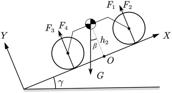
As shown in Figure 3, we establish the torque equations around point O in the X and Y directions on the plane; we can obtain the support force satisfying

$$\left\{\begin{array}{c}\sum F_i=F_M\hfill \\ (F_1+F_2)d-(F_3+F_4)d+G{h}_{2}sin\gamma sin\beta =0\hfill \\ (F_1+F_3)d-(F_2+F_4)d+G{h}_{2}sin\gamma cos\beta =0\hfill \end{array}\right.$$

(15)

Figure 3. Force analysis of the robot on an inclined wall surface.

The support forces acting on each magnetic wheel are denoted as $F_i$. $h_2$ represents the perpendicular distance from the mass center of the DSWCR to the wall surface, and $F_M$ represents the total adhesion force of each magnetic wheel.

The support force acting on each driving wheel can be calculated as follows:

$$\left\{\begin{array}{c}{F}_1=F_2={\displaystyle \frac{h_2(F_x-Gsin\gamma sin\beta )}{4d}}\hfill \\ F_3=F_4=-{\displaystyle \frac{h_2(F_x-Gsin\gamma sin\beta )}{4d}}\hfill \end{array}\right.$$

(16)

where $G{h}_{2}sin\psi sin\beta$ represents the component of gravity along the X direction. $F_x$ represents the inertial force along the X direction.

Similarly, we can write the equation for the robot along the Y direction:

$$\left\{\begin{array}{c}{F}_1=F_3={\displaystyle \frac{h_2(F_y-Gsin\gamma cos\beta )}{4b}}\hfill \\ F_2=F_4=-{\displaystyle \frac{h_2(F_y-Gsin\gamma cos\beta )}{4b}}\hfill \end{array}\right.$$

(17)

where $G{h}_{2}sin\psi cos\beta$ represents the component of gravity along the Y direction. $F_y$ represents the inertial force along the Y direction.

Combining Equations (16) and (17), we can obtain the corresponding support force for each magnetic wheel as follows:

$$\left\{\begin{array}{c}{F}_1={\displaystyle \frac{1}{4}}[F_M+h_2({\displaystyle \frac{F_x}{d}}+{\displaystyle \frac{F_y}{b}}-{\displaystyle \frac{Gsin\gamma sin\beta }{d}}-{\displaystyle \frac{Gsin\gamma cos\beta }{b}})]\hfill \\ F_2={\displaystyle \frac{1}{4}}[F_M+h_2({\displaystyle \frac{F_x}{d}}-{\displaystyle \frac{F_y}{b}}-{\displaystyle \frac{Gsin\gamma sin\beta }{d}}+{\displaystyle \frac{Gsin\gamma cos\beta }{b}})]\hfill \\ F_3={\displaystyle \frac{1}{4}}[F_M+h_2(-{\displaystyle \frac{F_x}{d}}+{\displaystyle \frac{F_y}{b}}+{\displaystyle \frac{Gsin\gamma sin\beta }{d}}-{\displaystyle \frac{Gsin\gamma cos\beta }{b}})]\hfill \\ F_4={\displaystyle \frac{1}{4}}[F_M+h_2(-{\displaystyle \frac{F_x}{d}}-{\displaystyle \frac{F_y}{b}}+{\displaystyle \frac{Gsin\gamma sin\beta }{d}}+{\displaystyle \frac{Gsin\gamma cos\beta }{b}})]\hfill \end{array}\right.$$

(18)

where $F_x$ and $F_y$ represent the total inertial forces along the X and Y directions, explicitly defined as $F_x=m{\ddot{x}}_O$ and $F_y=m{\ddot{y}}_O$ (with m being the total mass and ${\ddot{x}}_O,{\ddot{y}}_O$ being the accelerations of the center of mass). It is worth noting that a mathematical algebraic loop exists when computing the friction forces in a simulation, as $F_i$ depends on the accelerations, while the system accelerations depend on the friction derived from $F_i$. Inspired by the practical treatments in the recent literature [11], this dependence is effectively resolved in our simulation and control implementation by introducing a one-step numerical delay. Specifically, the accelerations from the previous time step are utilized to compute $F_x$ and $F_y$ for the current step. Due to the small discretization step size, this method accurately evaluates the real-time support forces without a computational singularity.

Substituting Equation (18) into Equation (15), we can verify that the obtained support forces satisfy the constraint Equation (15).

Next, we analyze the traction force of the magnetic wheel under the slip effect. We define the total longitudinal displacement of the wheel as ${\rho }_i=r{\dot{\alpha }}_i-\dot{\zeta }$. From ${\rho }_i$, we can obtain the slip ratio $s_i$ and slip angle ${\alpha }_i$. The expressions are as follows:

$$\begin{array}{c}{s}_i={\displaystyle \frac{r{\dot{\alpha }}_i-{\dot{\rho }}_i}{\max (\left|r{\dot{\alpha }}_i\right|,\left|{\dot{\rho }}_i\right|)}}={\displaystyle \frac{{\dot{\zeta }}_i}{\max (\left|r{\dot{\alpha }}_i\right|,\left|{\dot{\rho }}_i\right|)}}\hfill \\ {\alpha }_i=\mathrm{atan}({\displaystyle \frac{{\dot{\eta }}_i}{\left|r{\dot{\alpha }}_i-r{\dot{\zeta }}_i\right|}})\hfill \end{array}$$

(19)

where ${\zeta }_i$ and ${\eta }_i$ represent the lateral and longitudinal slip displacements generated by the i-th magnetic wheel, respectively.

We can model the relationship between traction forces and the slip ratio and slip angle using the simplified Dugoff model [34], which yields the following expressions:

$$\begin{array}{c}{F}_{Ri}=\sqrt{{(C_{xi}{s}_i)}^2+{(C_{yi}{\alpha }_i)}^2}\hfill \\ f_i=\left\{\begin{array}{c}1,F_{Ri}\le {\displaystyle \frac{u_i{F}_{zi}}{2}}\\ (2-{\displaystyle \frac{u_i{F}_{zi}}{2F_{Ri}}})({\displaystyle \frac{u_i{F}_{zi}}{2F_{Ri}}}),F_{Ri}>{\displaystyle \frac{u_i{F}_{zi}}{2}}\end{array}\right.\hfill \\ F_{lo{n}_i}=f_i{C}_{xi}{s}_i\hfill \\ F_{lati}=f_i{C}_{yi}{\alpha }_i\hfill \end{array}$$

(20)

where $C_{xi}$ and $C_{yi}$ represent the lateral and longitudinal stiffness of the wheel; $F_{zi}=F_i$ represents the normal load applied to the wheel, which is calculated by Equation (18); and $u_i$ represents the maximum rolling friction coefficient.

The simplified Dugoff model is adopted due to its suitability for the specific operating conditions of the magnetic DSWCR because the DSWCR operates at low, steady speeds with strong magnetic adhesion, which constrains the wheel slip ratios and slip angles within a small, linear region. Additionally, the dominant and predictable normal loads (comprising gravity and magnetic forces) allow for accurate real-time calculation. Within this linear slip regime, the simplified Dugoff model effectively captures the nonlinear coupling of longitudinal and lateral forces. Importantly, it significantly reduces the computational overhead compared to highly parameterized empirical models, thereby satisfying the strict real-time execution requirements of the adaptive dynamic programming (ADP) algorithm.

In conclusion, the calculation of the generalized forces Q acting on the DSWCR can be done as follows:

$$\begin{array}{ccc}\hfill Q= [& 00({\tau }_2-{\tau }_1-f_2{N}_2+f_1{N}_1)h_1\hfill & ({\tau }_4-{\tau }_3-f_4{N}_4+f_3{N}_3)h_{1}0\hfill \\ & {\tau }_1-f_1{N}_1{\tau }_2-f_2{N}_2{\tau }_3-f_3{N}_3\hfill & {\tau }_4-f_4{N}_4{]}^T\hfill \end{array}$$

(21)

where $h_1=b/r$ and drive torque $T=u_c={[{\tau }_1,{\tau }_2,{\tau }_3,{\tau }_4]}^T$. The matrix Q can be expressed in the form $E{u}_c+N$, where matrices E and N are

$$E={\left[\begin{array}{cc}{0}_{4\times 5}& I_{4\times 4}\end{array}\right]}^T, N={[\begin{array}{ccccc}{0}_{1\times 5}& -f_1{N}_1& -f_2{N}_2& -f_3{N}_3& -f_4{N}_4\end{array}]}^T$$

(22)

Substituting Equations (11), (13), (14) and (21) into Equation (10), we can obtain the dynamic model of the DSWCR. The specific matrix can be found in Appendix A. The dynamic model is as follows:

$$A(q)\ddot{q}+U(q,\dot{q})=Q+F^T(q)\lambda$$

(23)

Taking the time derivative of both sides of Equation (9), we can obtain

$$\ddot{q}=\dot{S}(q)(x(t)-\dot{\xi }(t))+S(q)(\dot{x}(t)-\ddot{\xi }(t))+\dot{\psi }(q,\dot{\eta })$$

(24)

Substituting Equation (24) into Equation (23) and multiplying both sides by $S^T(q)$ to eliminate the term $F^T(q)\lambda$, the dynamic model of the DSWCR can be expressed as follows:

$$M(q)\dot{x}+C(q,\dot{q})x+S^{T}U+W=S^{T}Q$$

(25)

where $M(q)=S^{T}AS$, $C(q,\dot{q})=S^{T}A\dot{S}$, and $W=-S^{T}A\dot{S}\dot{\zeta }-S^{T}A\dot{\psi }+\ddot{\zeta }$.

Combining the kinematic Equation (8) and the dynamic Equation (25), the model of the DSWCR can be transformed into a strict feedback form as follows:

$$\left\{\begin{array}{c}\dot{q}=S(q)x(t)+d_1\hfill \\ \dot{x}=f(q,x)+g(q,x)u_c+k(q,x)d_2\hfill \end{array}\right.$$

(26)

where $f(q,x)=-M^{-1}(Cx+S^{T}U), g(q,x)=M^{-1}, k(q,x)=-M^{-1}, d_1=-S(q)\dot{\xi }(t)+\psi (q,\dot{\eta }), d_2=-S^{T}A\dot{S}\dot{\zeta }-S^{T}A\dot{\psi }+\ddot{\zeta }$.

4. ADP Controller Based on Zero-Sum Game Theory

4.1. Trajectory Generation

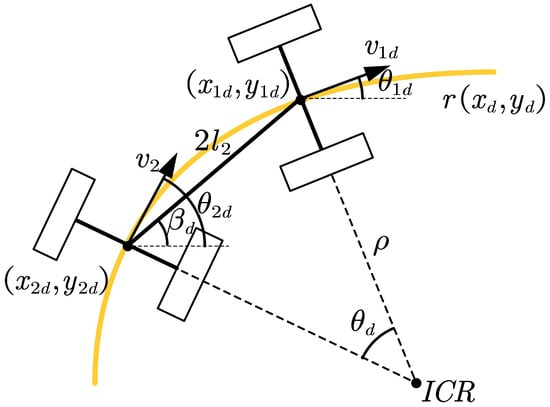
As shown in Figure 4, let us assume there is a predefined geometric path in the Cartesian plane with expression $r(x(t),y(t))$. It is necessary to establish a relationship between the reference trajectory and the state vector. We need to convert the reference trajectory into the desired state of the DSWCR at each moment. The desired state can be represented as $x_d(t)=[v_d(t),{\dot{\theta }}_{1d}(t),{\dot{\theta }}_{2d}(t)]$.

Figure 4. Reference trajectory generation.

From Equation (2), we can determine that the desired tangential velocity of the front body is $v_d=\sqrt{{\dot{x}}_{1d}^2+y_{1d}^2}$, and the desired steering angle is ${\theta }_{1d}=arctan({\dot{y}}_{1d}/{\dot{x}}_{1d})$. Taking the time derivative, we can obtain the corresponding desired steering angular velocity ${\dot{\theta }}_{1d}$ as

$${\dot{\theta }}_{1d}={\displaystyle \frac{{\dot{x}}_{1d}{\ddot{y}}_{1d}-{\dot{y}}_{1d}{\ddot{x}}_{1d}}{{\dot{x}}_{1d}^2+{\dot{y}}_{1d}^2}}$$

(27)

The desired position of $(x_{2d},y_{2d})$ satisfies the geometric relationship

$$\left\{\begin{array}{c}{x}_{2d}=x_{1d}-2dcos{\beta }_{2d}\\ y_{2d}=y_{1d}-2dsin{\beta }_{2d}\end{array}\right.$$

(28)

Similarly, we can obtain the desired angular velocity of the rear body as

$${\dot{\theta }}_{2d}={\displaystyle \frac{{\dot{x}}_{2d}{\ddot{y}}_{2d}-{\dot{y}}_{2d}{\ddot{x}}_{2d}}{{\dot{x}}_{2d}^2+{\dot{y}}_{2d}^2}}$$

(29)

The process of solving the desire angular velocity ${\dot{\theta }}_{2d}$ involves the yaw angle of the chassis $\beta$, which changes with the curvature of the curve. As shown in Figure 4, when both the front and rear bodies are moving on the desired trajectory, we can obtain the constraint from the geometric relationship

$$2dsin{\beta }_d=f(x_{1d}(t))-f(x_{1d}(t)-2dcos{\beta }_d)$$

(30)

From Equation (30), we can determine the desired yaw angle of the chassis at any time. By taking the time derivative of both sides of Equation (30), we can obtain the desired yaw angular velocity of the chassis as

$${\dot{\beta }}_d={\displaystyle \frac{\dot{f}[x_{1d}(t)]{\dot{x}}_{1d}(t)-\dot{f}[x_{1d}(t)-2dcos{\beta }_d]{\dot{x}}_{1d}(t)}{2dcos{\beta }_d+2dsin{\beta }_d\dot{f}(x_{1d}(t)-2dcos{\beta }_d)}}$$

(31)

Further differentiating with respect to ${\dot{\beta }}_d$, we can calculate ${\ddot{\beta }}_d$. Through the above equations, we can obtain the desired state of the robot at any time.

4.2. Optimal Controller Design for DSWCR

Tracking control aims to design a suitable controller for the DSWCR with uncertainties to make the tracking error e approach zero and maintain stability. In this section, we aim to achieve this goal by using an ADP controller based on zero-sum game theory. First, we define the tracking control system.

Considering the dynamic model of the DSWCR with uncertainties, we have

$$\dot{x}=f(q,x)+g(q,x)u_c+k(q,x)d$$

(32)

The desired state of the robot $x_d(t)$ is known. The error of the tracking system is defined as

$$e=x(t)+n(x)-x_d(t)$$

(33)

where $n(x)$ represents the state uncertainty, introduced from observation noise. Taking the time derivative of both sides of Equation (33), we obtain

$$\dot{e}=\dot{x}-{\dot{x}}_d=f(q,x,{\dot{x}}_d)+g(q,x)u_c+k(q,x)d+\Delta n(x)$$

(34)

where the system matrix $f\left(q,x,{\dot{x}}_d\right)=f(q,x)-{\dot{x}}_d$, $\Delta n(x)$ represents the change rate of state uncertainty, satisfying inequality $∥\Delta n(x)∥\le \Delta n_M∥e∥$. Meanwhile $g(q,x),k(q,x)$ are upper bounded, satisfying the inequality $∥g(q,x)∥\le g_M,∥k(q,x)∥\le k_M$; $g_M$, $k_M$, and $n_M$ are positive scalar constants [35].

Define the cost function [36] of the tracking system as follows:

$$V(e,u_c,d)={\int }_0^{\infty }(Q(e)+u_c^{T}R{u}_c-{\rho }^2{d}^{T}d+\Delta n_M∥e∥)d\tau$$

(35)

where $Q(e)=e^{T}Qe$ and Q and R are positive diagonal matrices. $\rho$ is a positive constant.

Considering the coexistence of control input and disturbance terms, the optimal control of the tracking system can be considered as a two-player zero-sum game problem, where the goal is to obtain the minimum cost function while the disturbance term reaches its maximum. The form of the two-player zero-sum game can be written as follows:

$$V^{\ast }(e,u_c,d)=\underset{u}{\min }c\underset{d}{\max }{\int }_0^{\infty }(Q(e)+u_c^{T}R{u}_c-{\rho }^2{d}^{T}d+\Delta n_M∥e∥)d\tau$$

(36)

To ensure the zero-sum game formulation is mathematically well-posed, it is assumed that the continuous external disturbance $d(t)$ is strictly bounded. Specifically, the disturbance belongs to an admissible constraint set $D=\{d\in {\mathbb{R}}^k: \parallel d(t)\parallel \le d_{max}\}$, where $d_{max}>0$ is a known upper bound. Furthermore, the negative quadratic penalty term $-{\gamma }^2{\parallel d\parallel }^2$ in the cost function ensures that the maximization problem with respect to $d(t)$ is strictly concave, yielding a unique and finite worst-case disturbance.

The Hamiltonian function of the system is as follows:

$$H(e,x,u_c,d)=Q(e)+u^{T}Ru-{\rho }^2{d}^{T}d+\Delta n_M∥e∥+\nabla V_e^T(f(e)+g(x)u_c+k(x)d)$$

(37)

where $\nabla V_e$ is the partial derivative of V with respect to e. By applying the optimality conditions ${\displaystyle \frac{\partial H}{\partial u_c}}=0$ and ${\displaystyle \frac{\partial H}{\partial d}}=0$, we can obtain the control and the disturbance input as follows:

$$\begin{array}{c}{\widehat{u_c}}^{\ast }(e)=\underset{u}{\arg \min } cH(e,u_c,d^{\ast },\nabla V_e^{\ast })=-{\displaystyle \frac{1}{2}}{R}^{-1}{g}^T(x)\nabla V_e^{\ast }(e)\hfill \\ {\widehat{d}}^{\ast }(e)=\underset{d}{\arg \max } H(e,u_c,d^{\ast },\nabla V_e^{\ast })={\displaystyle \frac{1}{2{\rho }^2}}{k}^T(x)\nabla V_e^{\ast }\hfill \end{array}$$

(38)

Substituting Equation (38) into Equation (37), we can obtain the another form of Hamilton:

$$\begin{array}{cc}\hfill & Q(e)-{\displaystyle \frac{1}{4}}\nabla V_e^{\ast T}(e)g(x)R^{-1}{g}^T(x)\nabla V_e^{\ast }(e)+\nabla V_e^{\ast T}f(e)+{\displaystyle \frac{1}{4{\rho }^2}}\nabla V_e^{\ast T}(e)\hfill \\ & k^T(x)k(x)\nabla V_e^{\ast }(e)+\Delta n_M∥e∥=0\hfill \end{array}$$

(39)

To obtain the optimal control input, we need to solve $\nabla V_e^{\ast }(e)$ in Equation (39). However, since Equation (39) is a nonlinear differential equation for $\nabla V_e^{\ast }(e)$, it is difficult to solve. Typically, online neural networks are employed to solve it.

4.3. Online Weight Update in Critic Network

In this section, the online weight update in critic network will be used to solve the HJI equation. Before that, Lemma 1 needs to be introduced.

Assumption 1 

([37]). Let $L(e)$ be a Lyapunov function for the DSWCR system (34) that satisfies the inequality

$$\dot{L}(e)=\nabla L_e^T(f(e)+g(x)u)<0$$

(40)

where $\nabla L_e^T$ is the partial derivative of $L(e)$ with respect to e. Meanwhile, there exists a positive diagonal matrix $\Lambda (e)$ satisfying

$$\nabla L_e^T(f(e)+g(x)u)=-\nabla L_e^T\Lambda (e)\nabla L_e$$

(41)

Assume that $∥f(e)+g(x)u∥\le \eta$ [38,39]. $f(e)+g(x)u$ can be assumed to be bounded by a function of e such that

$$∥f(e)+g(x)u∥\le \eta ∥\nabla L_e∥$$

(42)

where $\eta >0,\nabla L_e^T(f(e)+g(x)u)<0$. It can be observed that Equation (41) defined in Assumption 1 is reasonable. We can define $L(e)$ as a suitable polynomial, and here we choose $L(e)={\displaystyle \frac{1}{2}}{e}^{T}e$, $\nabla L_e=e$.

We apply the neural network to estimate the cost function [40]. The cost function value and its partial derivative with respect to e can be written as

$$\begin{array}{c}{V}_e^{\ast }=W_c^T\phi (e)+\epsilon (e)\hfill \\ \nabla V_e^{\ast }=\nabla {\phi }_e^T{W}_c+\nabla {\epsilon }_e\hfill \end{array}$$

(43)

where $W_c\in R^N$ represents the ideal weight of the critic network, N represents the number of neurons, $\phi (e)\in R^N$ represents the nonlinear activation function, and $\epsilon (e)$ represents the estimation error.

Assumption 2. 

For all admissible states x, the disturbance attenuation level ρ and the control weight matrix R are selected such that ${\lambda }_{min}(g(x)R^{-1}{g}^T(x))>{\displaystyle \frac{1}{{\rho }^2}}{\lambda }_{max}(k(x)k^T(x))$. This ensures that the matrix $G=g(x)R^{-1}{g}^T(x)-{\displaystyle \frac{1}{{\rho }^2}}k(x)k^T(x)$ remains strictly positive definite.

Substituting Equation (43) into Equation (39), the HJI equation can be rewritten as follows:

$$H(e,W)=Q(e)+W_c^T\nabla {\phi }_{e}f(e)-{\displaystyle \frac{1}{4}}{W}_c^T\nabla {\phi }_{e}G\nabla {\phi }_e^T{W}_c+\Delta n∥e∥+{\epsilon }_{HJB}$$

(44)

where $G=g(x)R^{-1}{g}^T(x)-{\displaystyle \frac{1}{{\rho }^2}}k(x)k^T(x)$ and $\rho$ is appropriately large to make G positive definite. ${\epsilon }_{HJB}$ represents the residual error of the HJI equation, and when N is appropriately large, ${\epsilon }_{HJB}$ converges to zero [41].

$${\epsilon }_{HJB}=\nabla {\epsilon }_e^T(f(e)+g(x)u_c^{\ast }+k(x)d^{\ast })+{\displaystyle \frac{1}{4}}\nabla {\epsilon }_e^{T}G\nabla {\epsilon }_e$$

(45)

When $N\to \infty$, the estimation error $\epsilon (e), \nabla {\epsilon }_e\to 0$ [42]. The ideal weight is represented by $W_c$, which is unknown; the estimate weight is represented by ${\widehat{W}}_c$. The estimates of $\widehat{V}(e)$, $\nabla {\widehat{V}}_e$, ${\widehat{u}}_c(e)$ and $\widehat{d}(e)$ can be written as follows:

$$\begin{array}{c}\widehat{V}(e)={{\widehat{W}}_c}^T\phi (e),\nabla \widehat{V}(e)=\nabla {\phi }_e^T{\widehat{W}}_c\hfill \\ {\widehat{u}}_c(e)=-{\displaystyle \frac{1}{2}}{R}^{-1}{g}^T(x)\nabla {\phi }_e^T{\widehat{W}}_c\hfill \\ \widehat{d}(e)={\displaystyle \frac{1}{2{\rho }^2}}{k}^T(x)\nabla {\phi }_e^T{\widehat{W}}_c\hfill \end{array}$$

(46)

Substituting Equation (46) into Equation (44), we can obtain the approximate Hamiltonian function:

$$\widehat{H}(e,{\widehat{W}}_c)=Q(e)+{\widehat{W}}_c^T\nabla {\phi }_{e}f(e)-{\displaystyle \frac{1}{4}}{\widehat{W}}_c^T\nabla {\phi }_{e}G\nabla {\phi }_e^T{\widehat{W}}_c+\Delta n∥e∥\stackrel{\Delta }{=}{e}_c$$

(47)

To obtain the ideal weights, it is necessary to minimize the error $e_c$. The optimal function is defined as $E={\displaystyle \frac{1}{2}}{e}_c^T{e}_c$. Referring to the study [43], the update of the weights is designed as

$$\begin{array}{c}\dot{{\widehat{W}}_c}(t)=-{\alpha }_1\varphi [Q(e)+\Delta n_M∥e∥+{{\widehat{W}}_c}^T\nabla {\phi }_{e}f(e)-{\displaystyle \frac{1}{4}}{{\widehat{W}}_c}^T\nabla {\phi }_{e}G(\widehat{x})\nabla {\phi }_e^T{\widehat{W}}_c]\hfill \\ +{\alpha }_2\Gamma (\widehat{x},{\widehat{u}}_c)\nabla {\phi }_{e}G\nabla L_e\hfill \end{array}$$

(48)

where learning rate ${\alpha }_1>0$, ${\alpha }_2>0$, $\varphi ={\displaystyle \frac{\sigma }{{({\sigma }^T\sigma +1)}^2}}$, $\sigma =\nabla {\phi }_e(f(e)-{\displaystyle \frac{1}{2}}G{\nabla }^T{\phi }_e{\widehat{W}}_c)$. The function expression $\Gamma (\widehat{x},\widehat{u})$ is as follows:

$$\Gamma (\widehat{x},{\widehat{u}}_c)=\left\{\begin{array}{c}0,\nabla L_e^T(f(e)-{\displaystyle \frac{1}{2}}G\nabla {\phi }_e^T{\widehat{W}}_c)<0\hfill \\ 1,otherwise\hfill \end{array}\right.$$

(49)

5. Stability and Convergence Proof

5.1. Convergence Analysis

Assumption 3 

([37]). The estimate error $\epsilon (e)$ and its partial derivative $\nabla {\epsilon }_e$ and the partial derivative of the activation function $\nabla {\phi }_e$ satisfy the inequalities $∥\epsilon (e)∥\le {\epsilon }_M$, $∥\nabla {\epsilon }_e∥\le \nabla {\epsilon }_M$, and $∥\nabla {\phi }_e∥\le \nabla {\phi }_M$. $\varphi ,\sigma ,{\epsilon }_{HJB}$ satisfy the inequalities $∥\varphi ∥\le {\varphi }_M$, $∥\sigma ∥\le {\sigma }_M$, and $∥{\epsilon }_{HJB}∥\le {\epsilon }_{HM}$. Matrix G is bounded and satisfies $G_m\le ∥G∥\le G_M$. Weight $W_c$ satisfies the inequality $∥W_c∥\le W_M$. ${\epsilon }_M$, $\nabla {\epsilon }_M$, $\nabla {\phi }_M$, ${\varphi }_M$, $G_m$, $G_M$, and $W_M$ are positive constants.

Theorem 1. 

For the DSWCR tracking system (34), when the control input $\widehat{u}$, disturbance $\widehat{d}$, and estimate weight ${\widehat{W}}_c$ are updated according to Equations (46) and (48), the weight estimate error $\tilde{W}$ will be uniform ultimately bounded (UUB).

Proof. 

Define the weight estimate error ${\tilde{W}}_c=W_c-{\widehat{W}}_c$. Differentiating both sides and substituting into Equations (44) and (48), we obtain

$$\dot{{\tilde{W}}_c}=-{\alpha }_1\varphi \sigma {\tilde{W}}_c^T-{\alpha }_1\varphi [{\displaystyle \frac{1}{4}}{\tilde{W}}_c^T\nabla {\phi }_{e}G\nabla {\phi }_e^T{\tilde{W}}_c+{\epsilon }_{HJB}]-{\alpha }_2\Gamma \nabla {\phi }_{e}G\nabla L_e$$

(50)

Define $L_1={\displaystyle \frac{1}{2{\alpha }_1}}{\tilde{W}}^T\tilde{W}$, we can obtain that:

$$\begin{array}{cc}\hfill {\dot{L}}_1& =-\varphi \sigma {{\tilde{W}}_c}^T{\tilde{W}}_c-\varphi {{\tilde{W}}_c}^T[{\displaystyle \frac{1}{4}}{{\tilde{W}}_c}^T\nabla {\phi }_{e}G\nabla {\phi }_e^T{\tilde{W}}_c+{\epsilon }_{HJB}]-{\displaystyle \frac{{\alpha }_2}{{\alpha }_1}}\Gamma \nabla {\phi }_{e}G\nabla L_e\hfill \\ \hfill & \le -\varphi {\sigma }_M{∥{\tilde{W}}_c∥}^2-{\displaystyle \frac{{\varphi }_M}{4}}{∥{\tilde{W}}_c∥}^3\nabla {\phi }_M^2{G}_m-{\varphi }_M∥{\tilde{W}}_c∥{\epsilon }_{HM}\hfill \end{array}$$

(51)

It can be inferred that when $∥{\tilde{W}}_c∥>{\displaystyle \frac{2\sqrt{{\sigma }_M^2-\nabla {\phi }_M^2{G}_m{\epsilon }_{H}M}-2{\sigma }_M}{\nabla {\phi }_M^2{G}_m}}$, ${\dot{L}}_1<0$. The UUB of weight estimation error can be demonstrated through the Lyapunov theory. □

5.2. Stability Analysis

Theorem 2. 

For the DSWCR tracking system (34), when the control input $\widehat{u}$, disturbance $\widehat{d}$, and weights ${\widehat{W}}_c$ update are updated according to Equations (46) and (48), the tracking error e will be UUB.

Proof. 

Define the cost function $V(e,u_c,d)$ as the Lyapunov function for the DSWCR system Equation (34) such that $L_2=V(e,u_c,d)$. Taking its time derivative we can obtain

$${\dot{L}}_2=\nabla V_e^{\ast T}(f(e)+g(x){\widehat{u}}_c^{\ast }+{\widehat{d}}^{\ast }+\Delta n)$$

(52)

Combining with Equation (39), Equation (52) can be rewritten as follows:

$$\begin{array}{cc}\hfill {\dot{L}}_2=& -Q(e)+{\displaystyle \frac{1}{4}}\nabla V_e^{\ast T}g(x)R^{-1}{g}^T(x)\nabla V_e^{\ast }-{\displaystyle \frac{1}{4{\rho }^2}}\nabla V_e^{\ast T}\nabla V_e^{\ast }+\hfill \\ & \nabla {V_e^{\ast }}^{T}g(x){\widehat{u}}_c^{\ast }+\nabla {V_e^{\ast }}^T{\widehat{d}}^{\ast }+\nabla {V_e^{\ast }}^T\Delta n-\Delta n_M∥e∥\hfill \end{array}$$

(53)

Substituting Equation (54) into Equation (53), we obtain

$$\begin{array}{cc}\hfill {\dot{L}}_2& \le -{\lambda }_{\min }{∥e∥}^2+({\phi }_M{W}_M+\nabla {\epsilon }_M-1)\Delta n_M∥e∥+{\displaystyle \frac{1}{4}}{(\nabla {\phi }_M{W}_M+{\epsilon }_M)}^2{G}_M\hfill \\ \hfill & +({\phi }_M{W}_M+\nabla {\epsilon }_M)(g_M∥u_c^{\ast }∥+∥d^{\ast }∥+{\displaystyle \frac{1}{2}}{G}_M\nabla {\epsilon }_M+{\displaystyle \frac{1}{2}}{G}_M{\phi }_M∥\tilde{W}∥)\hfill \\ \hfill & \le -{\lambda }_{\min }{∥e∥}^2+\Pi ∥e∥+\Xi \hfill \end{array}$$

(54)

where $\Xi ={\displaystyle \frac{1}{4}}{({\phi }_M{W}_M+\nabla {\epsilon }_M)}^2{G}_M+({\phi }_M{W}_M+\nabla {\epsilon }_M)(g_M∥u^{\ast }∥+∥d^{\ast }∥+{\displaystyle \frac{1}{2}}{G}_M\nabla {\epsilon }_M+{\displaystyle \frac{1}{2}}{G}_M{\phi }_M∥\tilde{W}∥)$, $\Pi =({\phi }_M{W}_M+\nabla {\epsilon }_M-1)\Delta n_M$, and ${\lambda }_{\min }$ is the minimum eigenvalue of the matrix Q. When $∥e∥>{\displaystyle \frac{\Gamma -\sqrt{{\Gamma }^2+4{\lambda }_{\min }{\Lambda }_2}}{2{\lambda }_{\min }}}$, ${\dot{L}}_2<0$. It can be observed that when ${\lambda }_{\min }$ is appropriately large, it ensures that the convergence region of e is small. □

6. Simulation

6.1. Tracking Performance Indexes

This section proposes several indexes to evaluate the tracking performance of the proposed method, including the maximum absolute error $e_{\max }$ and the root mean square error (RMSE) $\sigma$ of the tracking error, defined as

$$e_{\max }={\displaystyle \frac{1}{3}}(\max (\left|e_1(t)\right|)+\max (\left|e_2(t)\right|)+\max (\left|e_3(t)\right|)$$

(55)

$$\sigma ={\displaystyle \frac{1}{3}}(\sqrt{{\displaystyle \frac{1}{t}}{\int }_0^t{e}_1^2(\tau )d\tau }+\sqrt{{\displaystyle \frac{1}{t}}{\int }_0^t{e}_2^2(\tau )d\tau }+\sqrt{{\displaystyle \frac{1}{t}}{\int }_0^t{e}_3^2(\tau )d\tau })$$

(56)

The RMSE $\Delta$ between the desired trajectory and the executed trajectory of the DSWCR point F is defined as

$$\Delta =\sqrt{{\displaystyle \frac{1}{t}}{\int }_0^t{d}^2(t)d\tau }$$

(57)

where $d(t)=\sqrt{{(x_1(t)-x_{1d}(t))}^2+{(y_1(t)-y_{1d}(t))}^2}$.

6.2. Simulation Setting

In this section, the effectiveness of the proposed control method is demonstrated through two simulations. Case one is static target tracking, where the desired trajectory is set as a circular curve with a radius of 2 m. By using Equations (27)–(31), the static state targets are obtained as $v_{1d}=1$, ${\dot{\theta }}_{1d}(t)=0.5$, and ${\dot{\theta }}_{2d}(t)=0.5$. Case two is dynamic target tracking, where the desired trajectory is a sine curve with an amplitude of a, a frequency of w, and the expression $y=asin(wt)$. t represents the simulation time. It can be derived that the desired state $\left[v_{1d}(t),{\dot{\theta }}_{1d}(t),{\dot{\theta }}_{2d}(t)\right]$ at any given time satisfies

$$\begin{array}{c}{v}_{1d}=\sqrt{1+aw{cos}^2(wt)}\hfill \\ {\dot{\theta }}_{1d}(t)={\displaystyle \frac{-a{w}^{2}sin(wt)}{1+aw{cos}^2(wt)}}\hfill \\ {\dot{\theta }}_{2d}(t)={\displaystyle \frac{-a{w}^{2}sin(wt)}{1+aw{cos}^2(wt)}}\hfill \end{array}$$

(58)

The parameters of the dynamic model are set as shown in Table 2.

Table 2. Dynamic model parameters.

Variable	Unit	Value	Variable	Unit	Value
$M_w$	kg	1.2	$I_w$	kg · m2	$7.35\times {10}^{-4}$
$M_f$	kg	2.0	$I_{wz}$	kg · m2	$13.75\times {10}^{-4}$
$M_r$	kg	2.0	$I_C$	kg · m2	$20.8\times {10}^{-4}$
$M_p$	kg	1.2	$I_f$	kg · m2	$10.8\times {10}^{-4}$
b	m	0.08	$I_b$	kg · m2	$10.8\times {10}^{-4}$
d	m	0.08	$h_2$	m	0.12
r	m	0.035	$F_M$	N	40
$u_{Mi}$	/	0.35	$h_1$	/	2.286

6.3. Simulation Results

6.3.1. Case1: Static Target Tracking

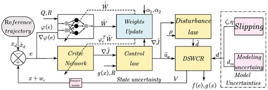
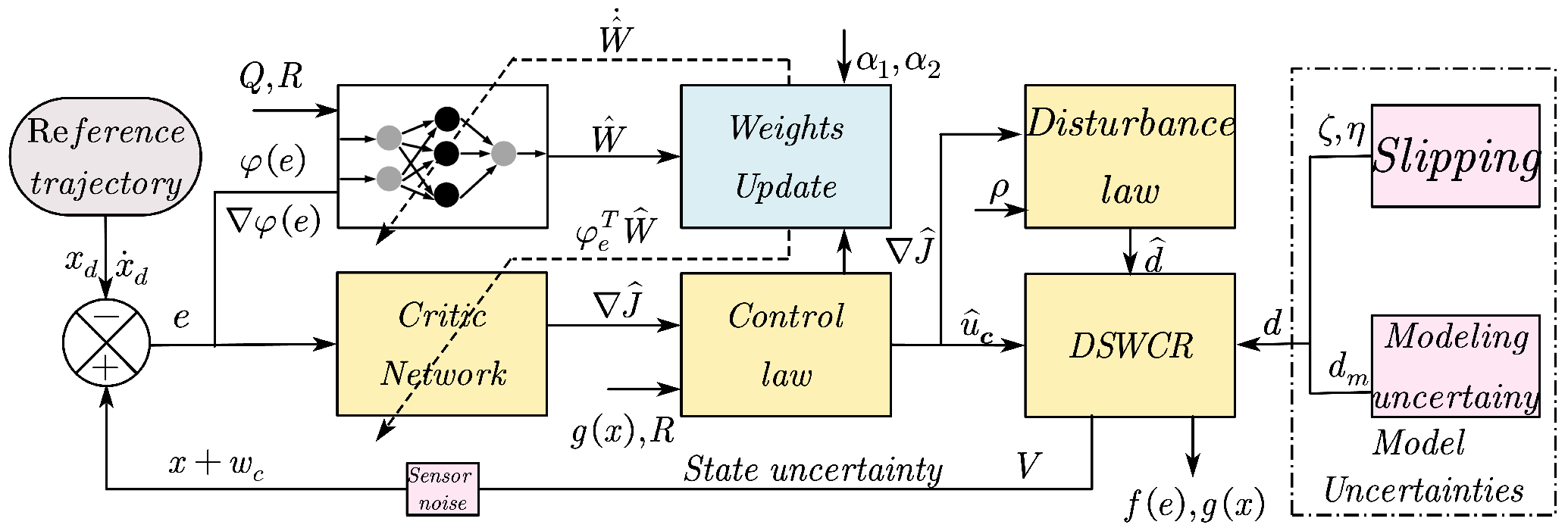
The structure of the controller is shown in Figure 5, with the initial settings of parameters as follows: the weight matrix of the cost function $Q=diag(1000,1000,1000)$, $R=diag(0.1,0.1,0.1)$. The time constant $t=0.01$ s, the threshold for the critic network ${\gamma }_d$ = 1 × 10⁻⁵, the learning rates in the network ${\alpha }_1=0.02$, ${\alpha }_2=0.01$, initial weights $Wc=rand()$, $rand()$ generated a random vecter within the interval $[-1,1]$, and the activation function $\phi (e)={[e_1,e_2,e_3,e_1^2/2,e_2^2/2,e_3^2/2,sin(e_1),sin(e_2),sin(e_3),tanh(e_1),tanh(e_2),tanh(e_3)]}^T$. The initial state of the DSWCR system is $V(0)=0;{\dot{\theta }}_1(0)=0;{\dot{\theta }}_2(0)=0$. During the simulation process, noise is added to the control input, denoted as $\zeta =rand(t)e^{-0.002t}$, to ensure a persistent excitation (PE) condition [44], and it is removed after the weights have converged.

Figure 5. The controller structure of the proposed method.

The proposed method will be compared with the PID and the Model Reference Adaptive Control (MRAC) method. The PID is incremental PD control with control parameters set as $k_p=[8.2,6.4,6.2]$, $k_d=[0.25,0.2,0.2]$. Referring to the literature [45,46], MRAC is designed in the following form:

$$\left\{\begin{array}{c}{\dot{x}}_m=A_m{x}_d+B_m{u}_r,u_r={\dot{x}}_d+K{x}_d\hfill \\ u_c=\Delta x+{\Delta }_r{u}_r\hfill \\ \dot{\Delta }=\overline{a}{w}_e{x}^T,{\dot{\Delta }}_r=\overline{b}{w}_e{u}_r^T\hfill \end{array}\right.$$

(59)

where $A_m=-K$, $B_m=I$, $K=diag[(1/dt;1/dt;1/dt)]$, and $w_e=Pe$, where P is a positive definite solution of the Lyapunov equation $A_m^{T}P+P{A}_m=-Q$. The adaptive gain is $\overline{a}=20$, $\overline{b}=0.32$.

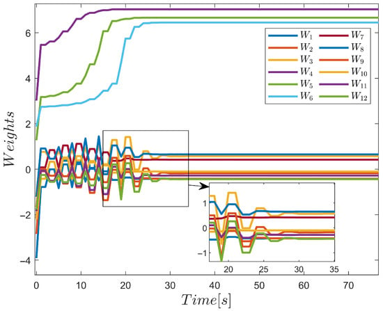
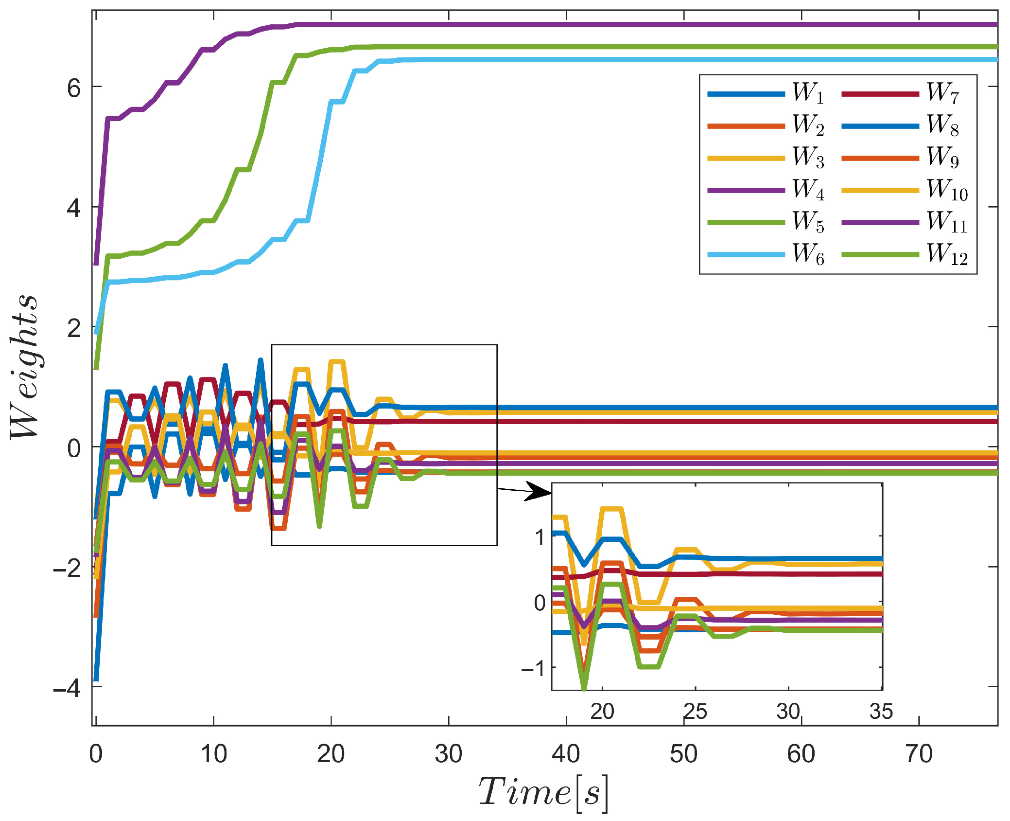
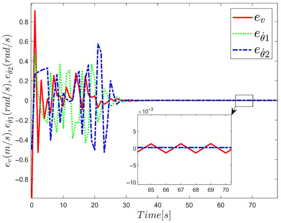
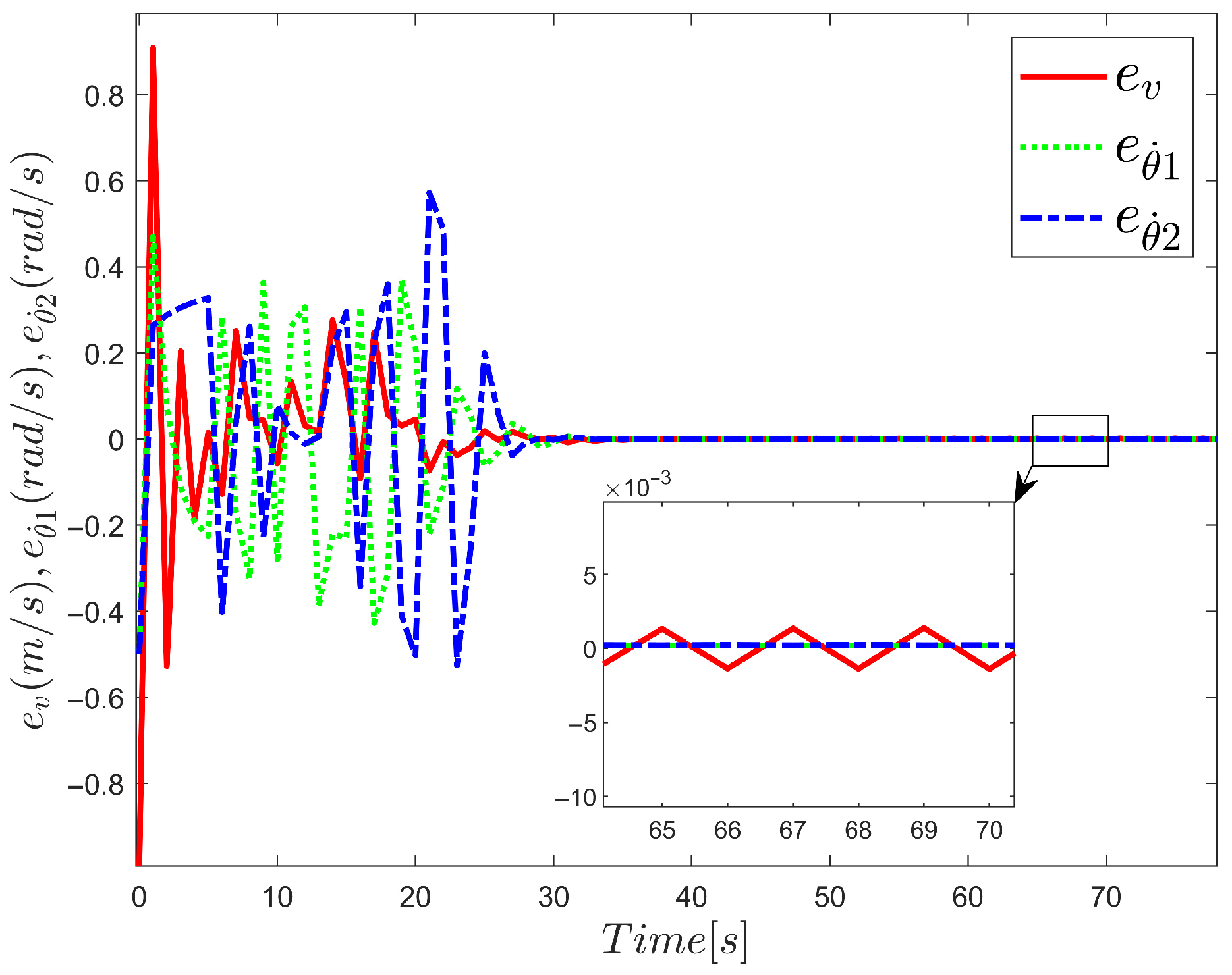
The weight updates of the critic network are shown in Figure 6. The weight values continue to update to reach the optimal value, and the weights converge to ${\widehat{W}}_c={[0.133,-0.998,-0.357,6.899,6.485,1.453,-0.471,0.268,0.500,0.238,0.679,-0.197]}^{\mathrm{T}}$. The tracking errors of the front body velocity and the angular acceleration of the front and rear bodies are shown in Figure 7. It can be observed that after the weight parameters converge, the tracking errors are controlled within a small range. The initial overshoot observed in Figure 7 is due to the lack of feasible control input during the initialization of the controller, which leads to an unstable state of the tracking control system. Although the neural network weights are continuously adjusted to make the initial controller the optimal controller, temporary overshoots or undershoots are unavoidable in the early stages.

Figure 6. Convergence of weights in critic network.

Figure 7. Curve of tracking error variation in static tracking.

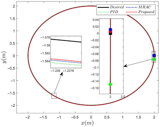
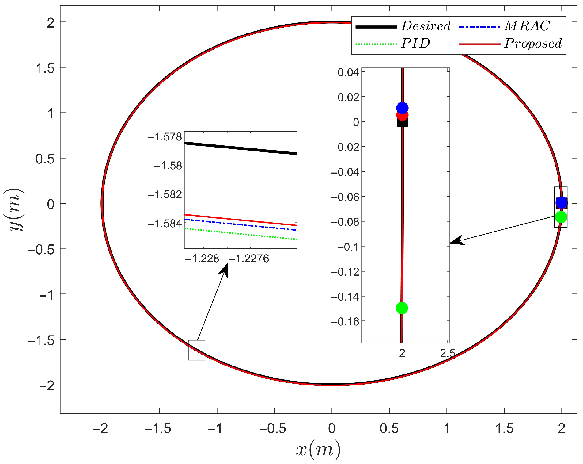
Figure 8 shows a comparison of the tracking performance among PID, MRAC, and the proposed method. The black line represents the desired trajectory, the green line represents the executed trajectory of the PID, the blue line represents the executed path of the MRAC, and the red line represents the executed trajectory of the proposed method. The DSWCR starts from the black square, with coordinates (2, 0). After moving along the circular curve, it reaches the circle points. PID, MRAC, and the proposed method reach the endpoints at (1.995, −0.1497), (2, 0.01085), and (2, 0.00547) respectively. The result shows that the ADP control method is closest to the endpoint.

Figure 8. Comparison of the executed trajectories among PID, MRAC, and the proposed method.

6.3.2. Case2: Dynamic Target Tracking

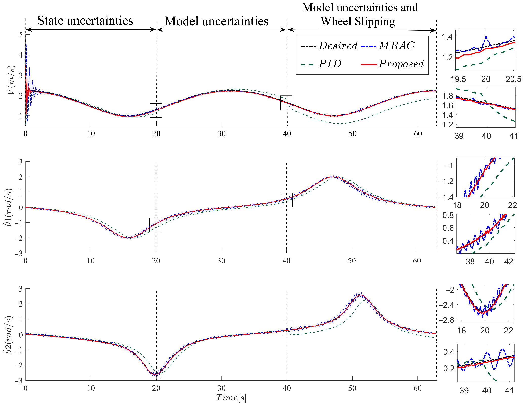
In the setup of the dynamic tracking simulation, special consideration was given to the influence of various uncertainties on the tracking performance. During the simulation process, the state uncertainty was represented by adding white noise to the observed state. The white noise consists of constant noise and Gaussian white noise. The constant white noise $n_d$ is set to 0.01. The Gaussian white noise $n_c$ follows a normal distribution with a mean of 0 and a variance of 0.01. The state uncertainty is added at the beginning of the simulation. The effects of slipping are considered as model uncertainty, and the slip variable is defined as a random variable:

$$\begin{array}{c}{\xi }_{l1}=a_{l1}{e}^{-nt}cos(nt),{\xi }_{r1}=a_{r1}{e}^{-nt}cos(nt),\hfill \\ {\xi }_{l2}=a_{l2}{e}^{-nt}cos(nt),{\xi }_{r2}=a_{r2}{e}^{-nt}cos(nt),\hfill \\ {\eta }_1=a_{\eta 1}{e}^{-nt}sin(nt),{\eta }_2=a_{\eta 2}{e}^{-nt}sin(nt)\hfill \end{array}$$

(60)

where the slip variable $a_{l1}=a_{l2}=1.5$, $a_{r1}=a_{r2}=1.2$, $a_{\eta 1}=a_{\eta 2}=0.5$, $n=2$. The model uncertainty caused by the slip is added after 20 s of simulation. In addition to the uncertainties mentioned above, the uncertainty caused by system modeling error needs to be considered as well. The uncertainty due to system modeling error is added after 40 s of simulation, denoted as ${\mathrm{d}}_m=q{[sin(\pi t/4)+cos(\pi t/4),sin(\pi t/2),cos(\pi t/2)]}^T$, where $q\in [-0.5,0.5]$. The initial settings of some parameters in the controller are modified: the desired trajectory parameters $a=2$, $w=1$, the threshold in the critic network ${\gamma }_d$ = 5 × 10⁻⁶, the learning rates ${\alpha }_1=0.012$, ${\alpha }_2=0.006$, and the uncertainty term $\Delta n_M=2$, $\rho =10$.

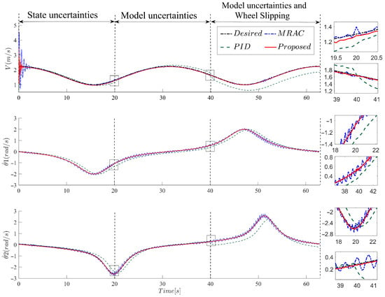
Figure 9 shows the comparison of the front body velocity, angular velocity, and rear body angular velocity tracking performance among PID, MRAC, and the proposed method under the influence of state and model uncertainties. During the first 0–4 s, the weights quickly converge, allowing accurate tracking in the presence of state uncertainty. Figure 9 demonstrates that the proposed method can effectively handle the model uncertainty after 20 s and the slip uncertainty after 40 s. However, PID is unable to handle the model uncertainties during the tracking process, while MRAC continuously adjusts its adaptive parameters, resulting in fluctuating states and inability to handle model uncertainties. The proposed method can eliminate the effects of uncertainties and achieve accurate tracking of the desired state.

Figure 9. Comparison of tracking performance among PID, MRAC, and the proposed method under uncertainties.

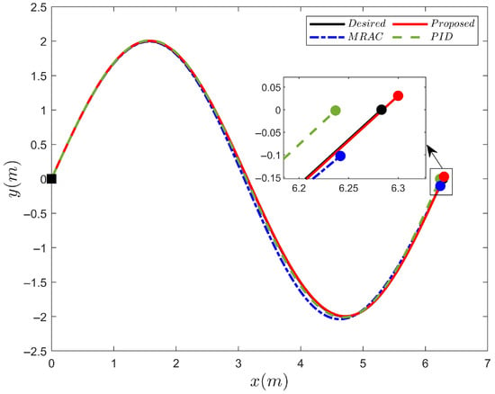
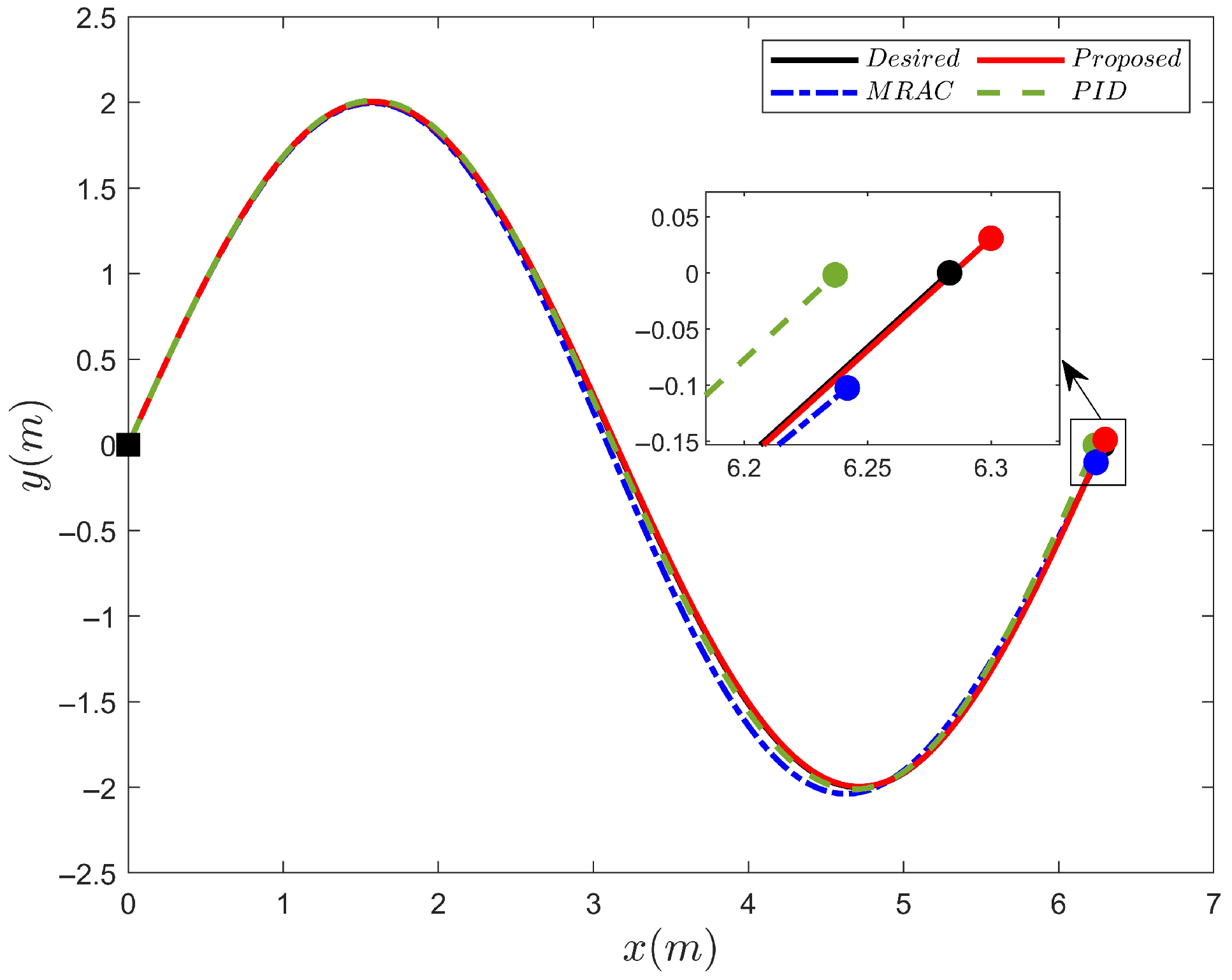
Figure 10 shows the comparison of executed trajectories among PID, MRAC, and the proposed method. From Figure 10, it can be observed that the DSWCR starts from the origin and moves along the sinusoidal curve. The red curve, representing the proposed method, is closest to the true trajectory represented by the black line. The endpoint coordinate of true trajectory is (6.283, 0), while the endpoints for PID, MRAC, and the proposed method are (6.237, −0.0018), (6.242, −0.1024), and (6.3, 0.03) respectively. The red point is closest to the endpoint.

Figure 10. Executed trajectories of PID, MRAC, and the proposed method.

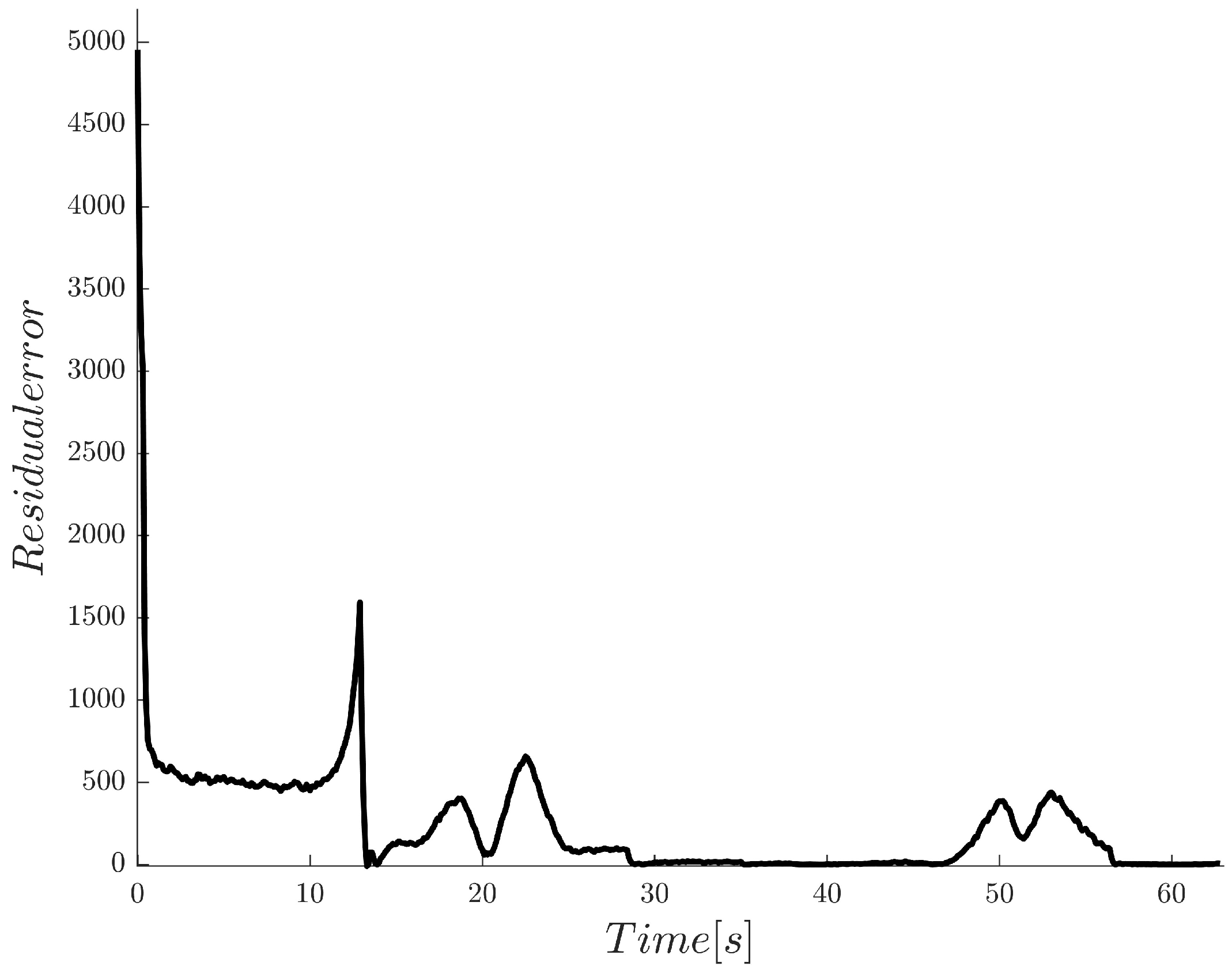
Figure 11 shows the process in which the residual error continuously decreases as the weights converge, ultimately reaching convergence with the residual error approaching 0. Table 3 shows a comparison of the tracking performance among PID, MRAC, and the proposed method without uncertainties and with uncertainties, evaluated using the index introduced in Section 5.1. From Table 3, it can be observed that the proposed method achieves the minimum values for the index $e_{\max }$, $\sigma$ and $\Delta$. The quantitative performance evaluation demonstrates that the proposed tracking method exhibits optimal tracking performance and maintains robustness against various uncertainties.

Figure 11. The change in residual error during the optimization process.

Table 3. Performance of tracking control under PID/MRAC/proposed.

Condition	Without Uncertain Term			With Uncertain Term
Index	$e_{\max }$	$\sigma$	$\Delta$	$e_{\max }$	$\sigma$	$\Delta$
PID	0.787	0.180	1.242	0.564	0.0762	0.734
MRAC	0.0531	0.0272	0.642	0.149	0.0335	0.103
Proposed	0.0322	0.0152	0.276	0.0736	0.0218	0.0761

7. Experimental Validation

7.1. Experimental Setup

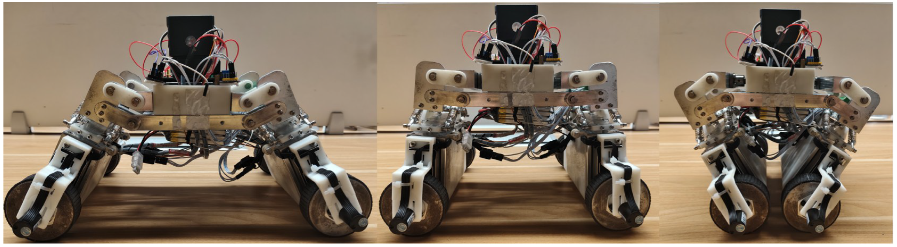
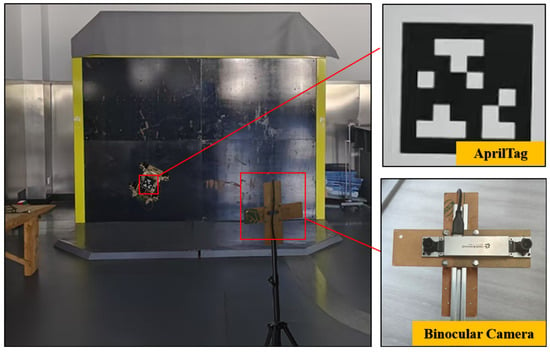
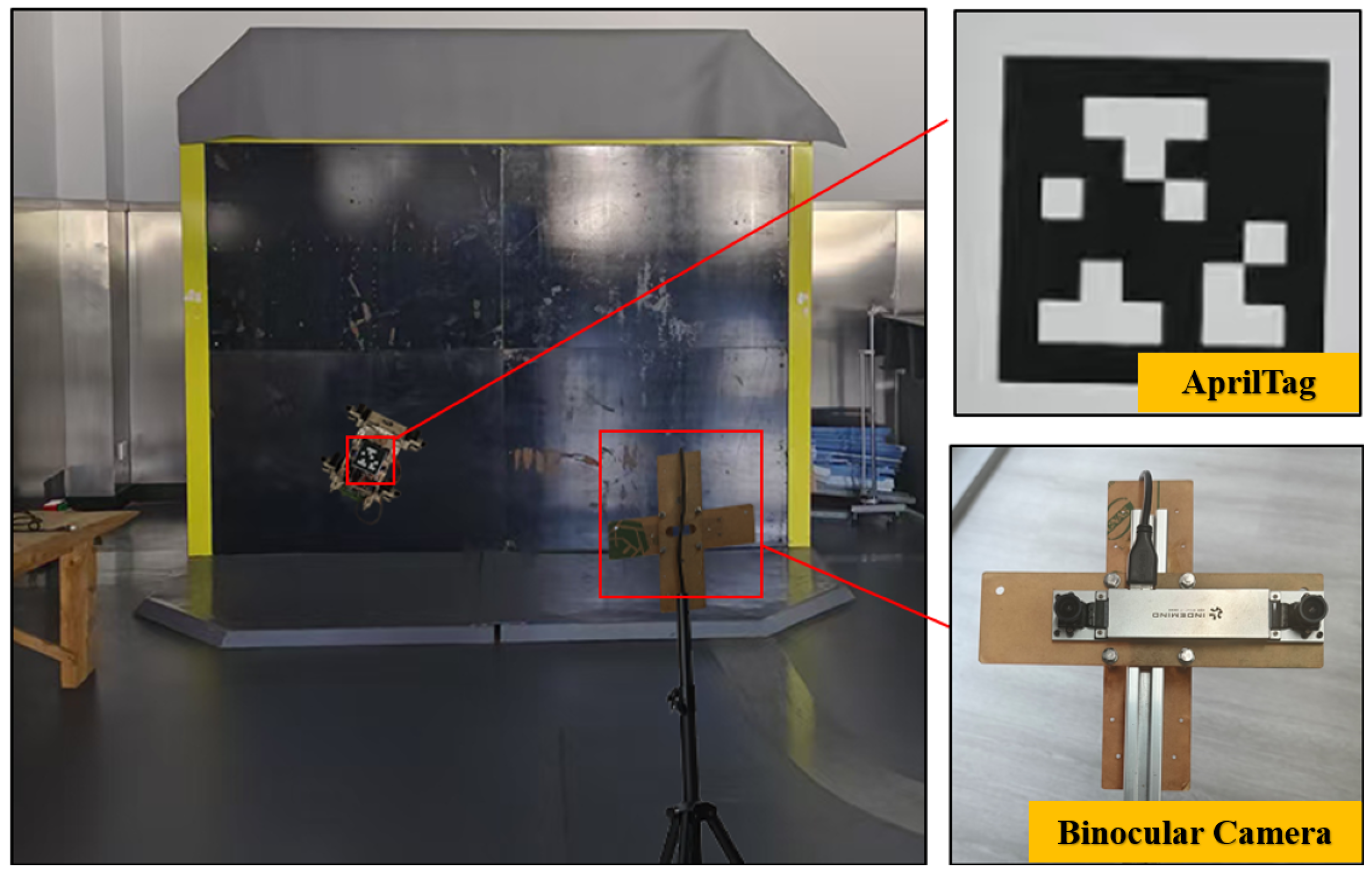
To further verify the engineering effectiveness and practical tracking performance of the proposed adaptive dynamic programming (ADP) controller, physical experiments were conducted. As shown in Figure 12 and Figure 13, the experimental platform was set up on a vertical steel plate measuring $500\mathrm{cm}\times 400\mathrm{cm}$. An AprilTag-based visual localization system was developed for real-time acquisition of the robot’s position. Specifically, an INDEMIND M1 binocular camera (resolution: $1280\times 800$; depth measurement range: $0.1$–$10\mathrm{m}$) was utilized for image capture and depth measurement, while a Tag36h11 fiducial marker ($10\mathrm{cm}\times 10\mathrm{cm}$) was firmly attached to the DSWCR chassis.

Figure 12. Prototype robot.

Figure 13. Experimental platform.

7.2. Trajectory Tracking and State Uncertainty Experiment

The robot was commanded to track a sinusoidal trajectory with an amplitude of $1\mathrm{m}$ at a constant speed of $5\mathrm{m}/\min$ to ensure consistent experimental conditions. The proposed ADP controller was compared with the Model Reference Adaptive Controller (MRAC) to evaluate tracking precision and disturbance rejection capabilities. Furthermore, to simulate state uncertainties typically encountered in complex industrial environments, Gaussian white noise was deliberately injected into the sensor measurement signals when the robot reached the midpoint of the path. This test was designed to evaluate the robustness of different control methods against sensor noise and measurement inaccuracies.

7.3. Model Uncertainty and Disturbance Experiment

To rigorously validate the robustness of the proposed ADP controller against severe model uncertainties, an additional set of experiments involving load variations, slip effects, and model noise was designed. Under the same tracking conditions ($5\mathrm{m}/\min$, tracking sine and square trajectories), the following dynamic disturbances were sequentially introduced to evaluate the tracking error, system response speed, and adaptive capacity of the ADP and MRAC methods:

• Initial Noise Disturbance: At the beginning of the experiment ($t=0\mathrm{s}$), random noise following a normal distribution was applied to the system model to simulate fundamental environmental uncertainties.
• Slip Displacement Interference: At $t=20\mathrm{s}$, artificial slip disturbances were introduced to force instantaneous displacement deviations, simulating the model uncertainty caused by non-ideal wheel–wall contact and loss of traction.
• Load Variation: At $t=40\mathrm{s}$, an additional payload of $2\mathrm{kg}$ was suddenly attached to the robot. This abrupt change was designed to test the self-adaptive capability of the controller when the mass and dynamic characteristics of the system undergo sudden mutations.

7.4. Experimental Results and Discussion

7.4.1. Tracking Performance Under State Uncertainties

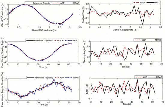
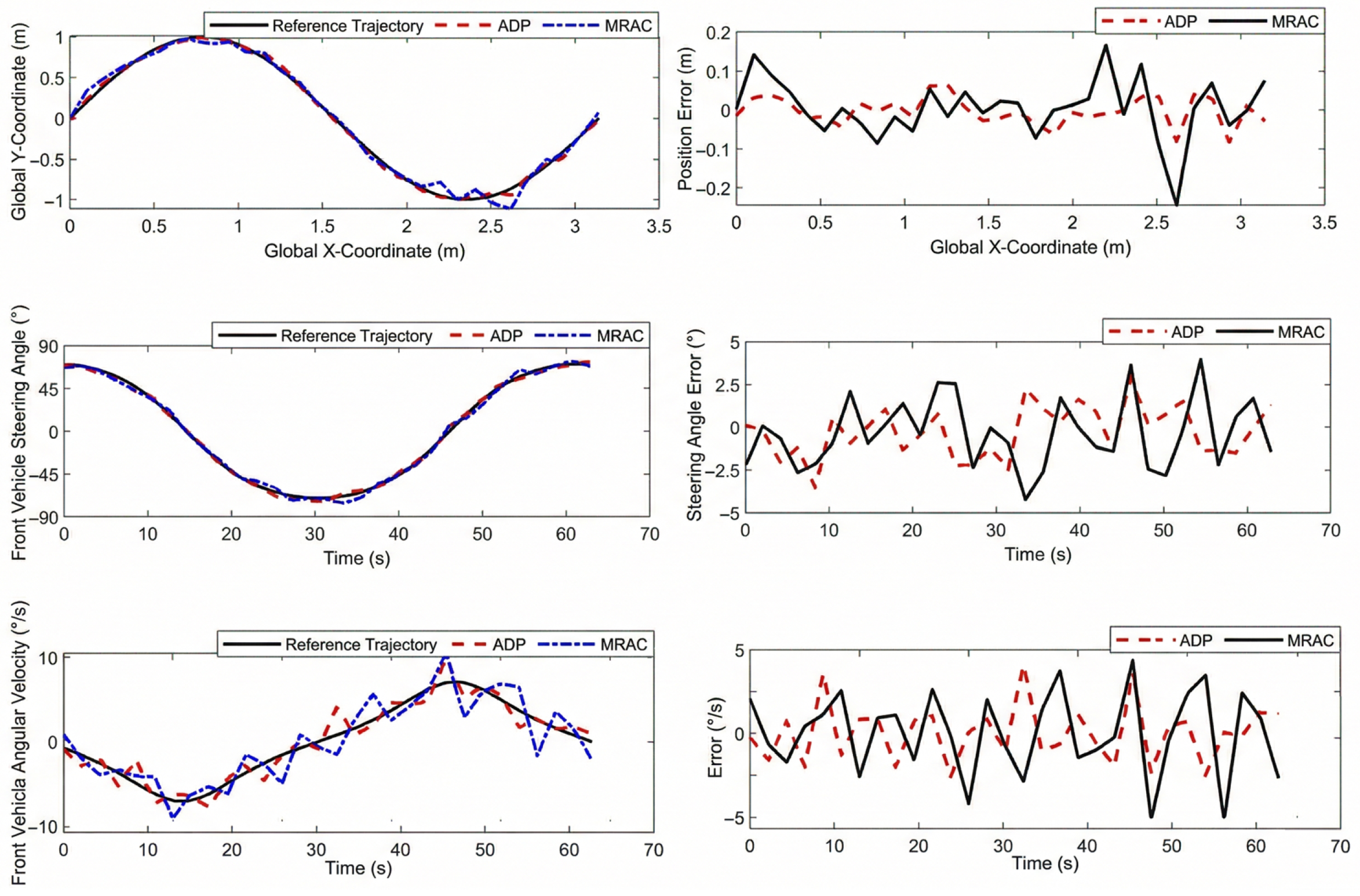
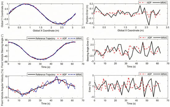
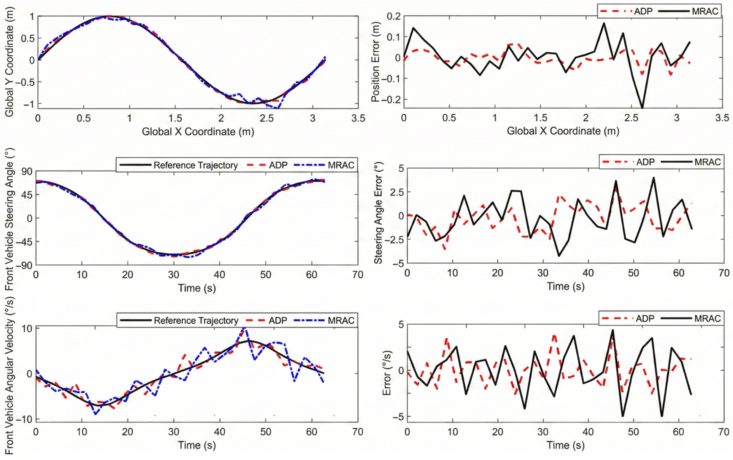
Figure 14 shows that before adding state uncertainties, both ADP and MRAC track the reference trajectory (solid black line) accurately. After adding the noise, MRAC shows large deviations. The ADP controller (red dashed line) keeps the position error within $\pm 0.1\mathrm{m}$. In contrast, the MRAC controller (blue dash-dotted line) fluctuates heavily, with a maximum error of $0.25\mathrm{m}$. This shows that ADP is more robust against state uncertainties.

Figure 14. Result of trajectory tracking and state uncertainty experiment.

For the steering angle, both controllers can generally follow the target. However, MRAC lags after the noise is added, especially at sharp turns. ADP adapts much better. The steering angle error of ADP stays within $\pm 2.5°$. Meanwhile, the MRAC error fluctuates drastically and exceeds $4.5°$. In short, ADP has smaller tracking errors, better steering precision, and smoother responses than MRAC.

7.4.2. Robustness Against Model Uncertainties

In the model uncertainty test, initial noise causes tracking errors for both methods. However, Figure 15 shows that ADP reduces the error and becomes stable much faster than MRAC.

Figure 15. Result of model uncertainty and disturbance experiment.

At $t=20\mathrm{s}$ (x-coordinate $\approx 1\mathrm{m}$), we introduce slip interference. Both trajectories deviate. ADP quickly adjusts its path and reduces the error. On the other hand, MRAC shows large error fluctuations and recovers slowly, especially near $x=1.5\mathrm{m}$.

At $t=40\mathrm{s}$, the sudden payload addition causes trajectory fluctuations for both methods. ADP adapts quickly to this load change and becomes stable again. MRAC adapts poorly, showing long and large error fluctuations.

In summary, ADP is much better at adapting and fixing errors caused by initial noise, slip, and load changes. Compared to MRAC, ADP has smaller errors and faster responses. This proves that ADP is highly robust and adaptable in complex, real-world environments.

8. Conclusions

In this paper, we established the dynamic model of the DSWCR based on the Lagrange equation. The model includes the effects of slip, the state uncertainty, and the model uncertainties. Then, we proposed an adaptive dynamic programming controller based on zero-sum game theory, which can accurately track the desired trajectory while maintaining robustness against uncertainties. Finally, through simulations and experimental validation, we demonstrated the robustness and optimality of the proposed method.

References

- Dai, Y.; Li, S.; Rui, X.; Xiang, C.; Nie, X. Review of key technologies of climbing robots. Front. Mech. Eng. 2023, 18, 48. [Google Scholar] [CrossRef] [Scilit]
- Fang, Y.; Wang, S.; Bi, Q.; Cui, D.; Yan, C. Design and technical development of wall-climbing robots: A review. J. Bionic Eng. 2022, 19, 877–901. [Google Scholar] [CrossRef] [Scilit]
- Tao, B.; Gong, Z.; Ding, H. Climbing robots for manufacturing. Natl. Sci. Rev. 2023, 10, nwad042. [Google Scholar] [CrossRef] [Scilit]
- Liu, Q.; Li, C.; Wang, G.; Li, L.; Wang, J.; Tan, J.; Wu, Y. Development of a Pipeline-Cleaning Robot for Heat-Exchanger Tubes. Electronics 2025, 14, 2321. [Google Scholar] [CrossRef] [Scilit]
- Hajeer, A.; Chen, L.; Hu, E. Review of classification for wall climbing robots for industrial inspection applications. In Proceedings of the 2020 IEEE 16th International Conference on Automation Science and Engineering (CASE), Hong Kong, China, 20–21 August 2020; IEEE: Piscataway, NJ, USA, 2020; pp. 1421–1426. [Google Scholar]
- Wang, C.; Zhu, S.; Song, W. Design and experiment of climbing robot for steel I-beam girder inspection. Ind. Robot. Int. J. Robot. Res. Appl. 2025, 52, 729–739. [Google Scholar] [CrossRef] [Scilit]
- Fan, H.; Zhu, S.; Wang, C.; Song, W. Modeling and Adaptive Neural Control of a Wheeled Climbing Robot for Obstacle-Crossing. Machines 2025, 13, 674. [Google Scholar] [CrossRef] [Scilit]
- Wang, B.; Li, P.; Li, P.; Zhang, L.; Guan, E.; Liu, X.; Hu, X.; Zhao, Y. Development of a wheeled wall-climbing robot with an internal corner wall adaptive magnetic adhesion mechanism. J. Field Robot. 2025, 42, 97–114. [Google Scholar] [CrossRef] [Scilit]
- Jiang, Z.; Zhao, Z.; Chen, B.; Li, Y.; Zhao, Y.; Xu, Y. Design and analysis of a passive adaptive wall-climbing robot based on five-bar mechanisms. Ocean. Eng. 2024, 298, 117140. [Google Scholar] [CrossRef] [Scilit]
- Lv, K.; Liu, Z.; Zhang, H.; Jia, H.; Mao, Y.; Zhang, Y.; Bi, G. Wheeled Permanent Magnet Climbing Robot for Weld Defect Detection on Hydraulic Steel Gates. Appl. Sci. 2025, 15, 7948. [Google Scholar] [CrossRef] [Scilit]
- Dian, S.; Fang, H.; Zhao, T.; Wu, Q.; Hu, Y.; Guo, R.; Li, S. Modeling and trajectory tracking control for magnetic wheeled mobile robots based on improved dual-heuristic dynamic programming. IEEE Trans. Ind. Inform. 2020, 17, 1470–1482. [Google Scholar] [CrossRef] [Scilit]
- Guizhi, L.; Peng, W.; Guohong, L.; Feng, L.; Shenglong, D. Dynamic modeling and analysis of wheeled wall-climbing robot. Adv. Mech. Eng. 2023, 15, 16878132231181247. [Google Scholar] [CrossRef] [Scilit]
- Santos, H.B.; Teixeira, M.A.S.; Dalmedico, N.; de Oliveira, A.S.; Neves, F., Jr.; Ramos, J.E.; de Arruda, L.V.R. Model predictive torque control for velocity tracking of a four-wheeled climbing robot. Sensors 2020, 20, 7059. [Google Scholar] [CrossRef] [Scilit]
- Chokshi, A.; Mehta, J.M. Dynamics of a four wheeled wall climbing robot. In Proceedings of the 18th International Conference on Informatics in Control, Automation and Robotics (ICINCO 2021), Online, 6–8 July 2021. [Google Scholar]
- Donglin, T.; Li, M.; Ding, C.; Wei, Z.; Hu, L.; Yua n, B. Research on steering stability of wheeled wall-climbing robot. Chin. J. Eng. Des. 2019, 26, 153. [Google Scholar]
- Hassan, I.A.; Abed, I.A.; Al-Hussaibi, W.A. Path Planning and Trajectory Tracking Control for Two-Wheel Mobile Robot. J. Robot. Control (JRC) 2024, 5, 1–15. [Google Scholar] [CrossRef] [Scilit]
- Morando, A.E.S.; Bozzi, A.; Graffione, S.; Sacile, R.; Zero, E. Optimizing Unmanned Air–Ground Vehicle Maneuvers Using Nonlinear Model Predictive Control and Moving Horizon Estimation. Automation 2024, 5, 324–342. [Google Scholar] [CrossRef] [Scilit]
- Kelley, L.; Ostovari, S.; Burmeister, A.B.; Talke, K.A.; Pezeshkian, N.; Rahimi, A.; Hart, A.B.; Nguyen, H.G. Design and experimental validation of a simple controller for a multi-segment magnetic crawler robot. In Proceedings of the Unmanned Systems Technology XVII; SPIE: Bellingham, WA, USA, 2015; Volume 9468, pp. 163–175. [Google Scholar]
- Liu, X.; Wang, Z.; Wu, J.; Wu, H.; Zhang, H. Trajectory Tracking of a Wall-Climbing Cutting Robot Based on Kinematic and PID Joint Optimization. Machines 2025, 13, 229. [Google Scholar] [CrossRef] [Scilit]
- Xie, F.; Mao, J.; Liu, Y.; Cao, L.; Song, G.; Song, A. Design and omnidirectional motion control of a circular concrete bridge pier climbing robot. Ind. Robot. Int. J. Robot. Res. Appl. 2025, 1–14. [Google Scholar] [CrossRef] [Scilit]
- Xiaojun, Z.; Yaqi, W.; Bicheng, X.; Jinliang, Z. Tracking control of wall climbing robot based on hybrid control algorithm. Comput. Integr. Manuf. Syst. 2023, 29, 3560. [Google Scholar]
- Xue, J.; Chen, J.; Stancu, A.; Wang, X.; Li, J. Spatial Trajectory Tracking of Wall-Climbing Robot on Cylindrical Tank Surface Using Backstepping Sliding-Mode Control. Micromachines 2023, 14, 548. [Google Scholar] [CrossRef] [Scilit]
- Zhang, D.; Li, Z.; Jia, P.; Zheng, Y.; Liu, S.; Wei, J.; Zhang, M.; Li, M. Optimization design and trajectory error compensation of a façade-adaptive wall-climbing robot. Symmetry 2023, 15, 255. [Google Scholar] [CrossRef] [Scilit]
- Chen, Z.; Liu, Y.; He, W.; Qiao, H.; Ji, H. Adaptive-neural-network-based trajectory tracking control for a nonholonomic wheeled mobile robot with velocity constraints. IEEE Trans. Ind. Electron. 2020, 68, 5057–5067. [Google Scholar] [CrossRef] [Scilit]
- Guo, Q.; Chen, Z. Neural adaptive control of single-rod electrohydraulic system with lumped uncertainty. Mech. Syst. Signal Process. 2021, 146, 106869. [Google Scholar] [CrossRef] [Scilit]
- Wang, G.; Ma, G.; Wang, D.; Bai, K.; Luo, W.; Zhuang, J.; Fan, Z. Real-Time Robotic Navigation with Smooth Trajectory Using Variable Horizon Model Predictive Control. Electronics 2026, 15, 603. [Google Scholar] [CrossRef] [Scilit]
- Szeremeta, M.; Szuster, M. Neural tracking control of a four-wheeled mobile robot with mecanum wheels. Appl. Sci. 2022, 12, 5322. [Google Scholar] [CrossRef] [Scilit]
- Wang, S.; Na, J. Parameter estimation and adaptive control for servo mechanisms with friction compensation. IEEE Trans. Ind. Inform. 2020, 16, 6816–6825. [Google Scholar] [CrossRef] [Scilit]
- Li, J.; Wang, J.; Peng, H.; Hu, Y.; Su, H. Fuzzy-torque approximation-enhanced sliding mode control for lateral stability of mobile robot. IEEE Trans. Syst. Man Cybern. Syst. 2021, 52, 2491–2500. [Google Scholar] [CrossRef] [Scilit]
- Tong, M.; Lin, W.; Huo, X.; Jin, Z.; Miao, C. A model-free fuzzy adaptive trajectory tracking control algorithm based on dynamic surface control. Int. J. Adv. Robot. Syst. 2020, 17, 1729881419894417. [Google Scholar] [CrossRef] [Scilit]
- Fang, H.; Zhu, Y.; Dian, S.; Xiang, G.; Guo, R.; Li, S. Robust tracking control for magnetic wheeled mobile robots using adaptive dynamic programming. ISA Trans. 2022, 128, 123–132. [Google Scholar] [CrossRef] [Scilit]
- Tian, Y.; Sidek, N.; Sarkar, N. Modeling and control of a nonholonomic wheeled mobile robot with wheel slip dynamics. In Proceedings of the 2009 IEEE Symposium on Computational Intelligence in Control and Automation, Nashville, TN, USA, 30 March–2 April 2009; IEEE: Piscataway, NJ, USA, 2009; pp. 7–14. [Google Scholar]
- Luy, N.T. Robust adaptive dynamic programming based online tracking control algorithm for real wheeled mobile robot with omni-directional vision system. Trans. Inst. Meas. Control 2017, 39, 832–847. [Google Scholar] [CrossRef] [Scilit]
- Habibnejad Korayem, M.; Ghobadi, N.; Fathollahi Dehkordi, S. Designing an optimal control strategy for a mobile manipulator and its application by considering the effect of uncertainties and wheel slipping. Optim. Control Appl. Methods 2021, 42, 1487–1511. [Google Scholar] [CrossRef] [Scilit]
- Kong, L.; Zhang, S.; Yu, X. Approximate optimal control for an uncertain robot based on adaptive dynamic programming. Neurocomputing 2021, 423, 308–317. [Google Scholar] [CrossRef] [Scilit]
- Szuster, M.; Hendzel, Z. Intelligent Optimal Adaptive Control for Mechatronic Systems; Springer: Berlin/Heidelberg, Germany, 2018. [Google Scholar]
- Wang, D.; Mu, C. A novel neural optimal control framework with nonlinear dynamics: Closed-loop stability and simulation verification. Neurocomputing 2017, 266, 353–360. [Google Scholar] [CrossRef] [Scilit]
- Bhasin, S.; Kamalapurkar, R.; Johnson, M.; Vamvoudakis, K.G.; Lewis, F.L.; Dixon, W.E. A novel actor–critic–identifier architecture for approximate optimal control of uncertain nonlinear systems. Automatica 2013, 49, 82–92. [Google Scholar] [CrossRef] [Scilit]
- Modares, H.; Lewis, F.L. Optimal tracking control of nonlinear partially-unknown constrained-input systems using integral reinforcement learning. Automatica 2014, 50, 1780–1792. [Google Scholar] [CrossRef] [Scilit]
- Vamvoudakis, K.G.; Lewis, F.L. Online actor–critic algorithm to solve the continuous-time infinite horizon optimal control problem. Automatica 2010, 46, 878–888. [Google Scholar] [CrossRef] [Scilit]
- Abu-Khalaf, M.; Lewis, F.L. Nearly optimal control laws for nonlinear systems with saturating actuators using a neural network HJB approach. Automatica 2005, 41, 779–791. [Google Scholar] [CrossRef] [Scilit]
- Mostovoy, J. Spaces of rational maps and the Stone–Weierstrass theorem. Topology 2006, 45, 281–293. [Google Scholar] [CrossRef] [Scilit]
- Liu, D.; Wei, Q.; Wang, D.; Yang, X.; Li, H. Adaptive Dynamic Programming with Applications in Optimal Control; Springer: Berlin/Heidelberg, Germany, 2017. [Google Scholar]
- Kong, L.; He, W.; Yang, C.; Sun, C. Robust neurooptimal control for a robot via adaptive dynamic programming. IEEE Trans. Neural Netw. Learn. Syst. 2020, 32, 2584–2594. [Google Scholar] [CrossRef] [Scilit]
- Shojaei, K.; Shahri, A.M.; Tarakameh, A.; Tabibian, B. Adaptive trajectory tracking control of a differential drive wheeled mobile robot. Robotica 2011, 29, 391–402. [Google Scholar] [CrossRef] [Scilit]
- Canigur, E.; Ozkan, M. Model reference adaptive control of a nonholonomic wheeled mobile robot for trajectory tracking. In Proceedings of the 2012 International Symposium on Innovations in Intelligent Systems and Applications, Trabzon, Turkey, 2–4 July 2012; IEEE: Piscataway, NJ, USA, 2012; pp. 1–5. [Google Scholar]
Disclaimer/Publisher’s Note: The statements, opinions and data contained in all publications are solely those of the individual author(s) and contributor(s) and not of MDPI and/or the editor(s). MDPI and/or the editor(s) disclaim responsibility for any injury to people or property resulting from any ideas, methods, instructions or products referred to in the content. |
© 2026 by the authors. Licensee MDPI, Basel, Switzerland. This article is an open access article distributed under the terms and conditions of the Creative Commons Attribution (CC BY) license.