A Resilient Ensemble Deep Learning Architecture for Load Forecasting Against FDI Attack

Abstract

Short-term load forecasting (STLF) is crucial for ensuring power grid stability and economic dispatch. Its accuracy heavily depends on the quality of the input data. However, collecting operational data via the power system’s communication network poses a significant vulnerability to cyberattacks, particularly stealthy False Data Injection (FDI) attacks. By closely mimicking normal load fluctuations, these attacks evade conventional detection, thus, compromising forecasting reliability. To address this challenge, this paper proposes a novel resilient load forecasting framework that integrates two-stage attack detection with robust ensemble learning. In the detection stage, attack identification is performed through seasonal decomposition and AE-BiLSTM reconstruction, followed by restoration using periodic-consistent historical means and secondary screening via second-order differencing (SOD). In the forecasting stage, an improved Multi-Objective Whale Migration Algorithm (MO-WMA) is employed to adaptively optimize ensemble weights for intelligent fusion, significantly enhancing prediction accuracy and robustness, and providing a generalizable solution for intelligent grid load forecasting. Experiments were conducted on the Independent System Operator of New England (ISO New England, 2012–2014) load dataset under four typical FDI attack scenarios, with test sets including diverse attack intensities and temporal patterns. Results show that the framework achieves $98.98\%$ attack detection accuracy and improves the $R^2$ forecasting metric from 0.9053 to 0.9851, approaching attack-free performance, demonstrating effective recovery of forecasting accuracy and generalization capability.

1. Introduction

Short-term load forecasting (STLF) serves as a critical foundation for decision-making in power system operations, where its accuracy directly influences grid security and stability [1]. However, operational data collected via power system communication networks is subject to serious threats from False Data Injection (FDI) attacks [2]. By tampering with measurement data, attackers can cause significant deviations in forecasting results, leading to operational dispatch failures [3]. The 2015 cyberattack on Ukraine’s power grid exemplifies the real-world damage caused by such threats [4]. Therefore, developing attack-resilient load-forecasting methods is essential to ensuring power system security.

To address this critical challenge, research efforts have primarily focused on FDI attack detection methods to enhance data quality for power system analysis. Existing approaches can be categorized into two groups: statistical methods and machine learning techniques approaches. Among statistical methods, Yue [5] introduced a hybrid detection mechanism. It combines second-order differencing with Chebyshev’s inequality for point-level anomaly detection. The method also incorporates the Heuristically Ordered Time-Symbolic Aggregate Approximation technique to capture subsequence-level anomalies. However, this method lacks an adaptive thresholding mechanism, limiting its adaptability under complex and varying operating conditions. As an improvement, Ref. [6] proposed a data-driven approach using Symbolic Aggregate Approximation to detect abnormal patterns in both load and meteorological data. Nevertheless, existing statistical methods generally overlook the inherent nonlinearity of load data, resulting in suboptimal performance on real-world datasets.

To address the challenge of capturing nonlinear features, machine learning-based detection methods have emerged. Existing studies have demonstrated that machine learning algorithms, when combined with large-scale electricity consumption data, exhibit strong generalization capability and significant potential in electricity anomaly detection tasks [7]. Building upon this foundation, various models—including Graph Neural Networks [8], Isolation Forest [9], Reinforcement Learning [10], and Long Short-Term Memory networks [11] have been widely applied in FDI attack detection. Notably, hybrid deep learning architectures demonstrate significant potential by integrating multiple technical advantages. For example, Cui et al. [12] developed a detection framework combining k-means clustering, Naive Bayes classification, and dynamic programming. Audibert et al. [13] proposed USAD, an unsupervised model based on adversarial autoencoders, to enhance generalization. Meanwhile, Wang et al. [14] established an unsupervised detection paradigm by comparing real-time load patterns with historical profiles. Furthermore, techniques such as multi-scale decomposition [15] and phase-space reconstruction [16] have been employed to explore intrinsic characteristics of load data. In recent years, as attack scenarios and data scales have become more complex, several emerging detection methods have been proposed. For example, Wang et al. [17] proposed a data-driven framework based on subspace identification for the detection and localization of FDI attacks. Wang et al. [18] proposed a recursive variational graph autoencoder, which enhances detection robustness under noisy measurement data by adding artificial noise during recursive training. However, despite the progress in attack detection accuracy, these methods share common limitations: most focus only on anomaly detection and lack mechanisms for repairing corrupted load data. As a result, under sustained attacks or large-scale data contamination, they struggle to provide reliable data for subsequent load forecasting, which can impact prediction accuracy and system security.

In response to these deficiencies, some studies have begun exploring collaborative detection and recovery mechanisms. Yue et al. [19] proposed a detection-replacement scheme using integrated solutions and their hybrid variants, but its performance deteriorates significantly with large-scale data corruption. Although the AE-CLSTM model developed by Moradzadeh et al. [20] reconstructs compromised data using autoencoders, the resulting over-smoothing ultimately constrains improvements in forecasting accuracy. These developments reveal that existing methods still face difficult trade-offs between achieving accurate detection and maintaining prediction performance.

In contrast to detection-replacement paradigms, another research direction focuses on developing inherently robust load forecasting models that can withstand data contamination directly. For instance, Luo et al. [21] established important benchmarks by conducting resilience testing across four representative models. Subsequent studies developed various robust regression methods, including improved models based on iteratively reweighted least squares and L1 regression [22], as well as adaptive robust regression incorporating M-estimation and adaptive least trimmed squares [23]. However, these linear-based methods perform inadequately when handling nonlinear load characteristics. To overcome this limitation, researchers have proposed nonlinear approaches, including Gaussian process regression, random forests [24], and non-kernel weighted quadratic surface support vector regression [25]. Recent advances include Li et al. [26]’s GenS2-P framework, which uses self-supervised data repair, and He et al. [27]’s ensemble support vector regression method, both of which demonstrate superior performance across various attack scenarios. Nevertheless, when confronting large-scale data contamination, these methods still experience significant accuracy degradation. Maintaining robustness while ensuring prediction accuracy remains a critical challenge.

In recent years, researchers have begun exploring hybrid strategies that integrate FDI detection methods with robust prediction models. For example, Ref. [28] proposed a robust load forecasting framework that first corrects corrupted data using an anomaly detection method based on a denoising variational autoencoder. Subsequently, the framework integrates IRLS with Huber robust regression to perform resilient load forecasting. However, this method fails to exploit the structural and periodic characteristics of load data fully, performs poorly in detecting attacks that resemble normal fluctuations, and still exhibits limited accuracy in data reconstruction and robust forecasting under large-scale attacks.

To address the limitations of existing methods, this paper proposes a detection-prediction collaborative framework. By integrating deep temporal modeling with multi-objective optimization algorithms, the approach achieves efficient detection of FDI attacks and robust short-term load forecasting. Specifically, this paper proposes a two-stage attack detection and recovery mechanism to address the limitations of existing methods, which often rely on a single component or external features and struggle to distinguish normal load fluctuations from abnormal attacks. This mechanism relies solely on the intrinsic temporal characteristics and periodic patterns of the load series to accurately identify and repair compromised data. Subsequently, a multi-objective whale migration algorithm (MO-WMA) is introduced to jointly optimize the ensemble weights of multiple forecasting models. Unlike traditional single-objective or heuristic weighting schemes, MO-WMA simultaneously balances diverse performance criteria, including forecasting accuracy and robustness against attack-induced disturbances. As a result, the proposed framework maintains high predictive reliability across diverse FDI attack scenarios. Overall, the method achieves a favorable trade-off between detection sensitivity and forecasting robustness, providing an innovative and practical solution for securing load forecasting in smart grid environments. Based on the above motivations, this study addresses the following research questions:

(1) How can stealthy FDI attacks that mimic normal load fluctuations be accurately detected using the intrinsic temporal and periodic characteristics of load data?

(2) How can short-term load forecasting performance be restored after FDI attack detection and data recovery?

The main contributions of this study are summarized as follows:

• This study develops a detection–prediction collaborative framework to enhance the resilience and security of the power load forecasting system.
• A two-stage FDI attack detection method, combining reconstruction after seasonal decomposition and second-order differencing (SOD), was developed, along with a data recovery strategy based on historical periodic means. This approach effectively enables the identification of attacks and significantly improves the accuracy of data restoration.
• An improved MO-WMA is employed to jointly optimize the ensemble weights of multiple forecasting models, enhancing both accuracy and robustness of the overall prediction performance.

To further clarify the methodological positioning and advantages of the proposed framework with respect to existing studies, Table 1 provides a comparative summary of representative FDI-related works and this paper in terms of detection capability, data recovery, and forecasting robustness.

Table 1. Comparison of Representative FDI Attack-related Studies and This Work.

Reference	FDI Detection	Data Recovery	Robust Forecasting	Large-Scale/Stealthy Attacks
Yue et al. (2017) [5]	✓	×	×	×
Yue et al. (2018) [6]	✓	×	×	×
Cui et al. (2019) [12]	✓	×	×	×
Audibert et al. (2020) [13]	✓	×	×	×
Wang et al. (2023) [14]	✓	×	×	×
Wang et al. (2025) [18]	✓	×	×	×
Moradzadeh et al. (2022) [20]	✓	✓	×	×
Zheng et al. (2020) [28]	✓	✓	✓	×
Luo et al. (2018) [22]	×	×	✓	×
Jiao et al. (2022) [23]	×	×	✓	×
Li et al. (2025) [26]	✓	✓	✓	×
This work	✓	✓	✓	✓

The remainder of this paper is organized as follows. Section 2 presents the problem description, and Section 3 constructs four typical attack templates. Section 4 outlines the proposed collaborative framework, which integrates attack detection and robust forecasting. Section 5 validates the effectiveness of the method through experimental results. Finally, Section 6 concludes the paper and discusses future research directions.

2. Problem Description

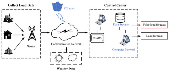
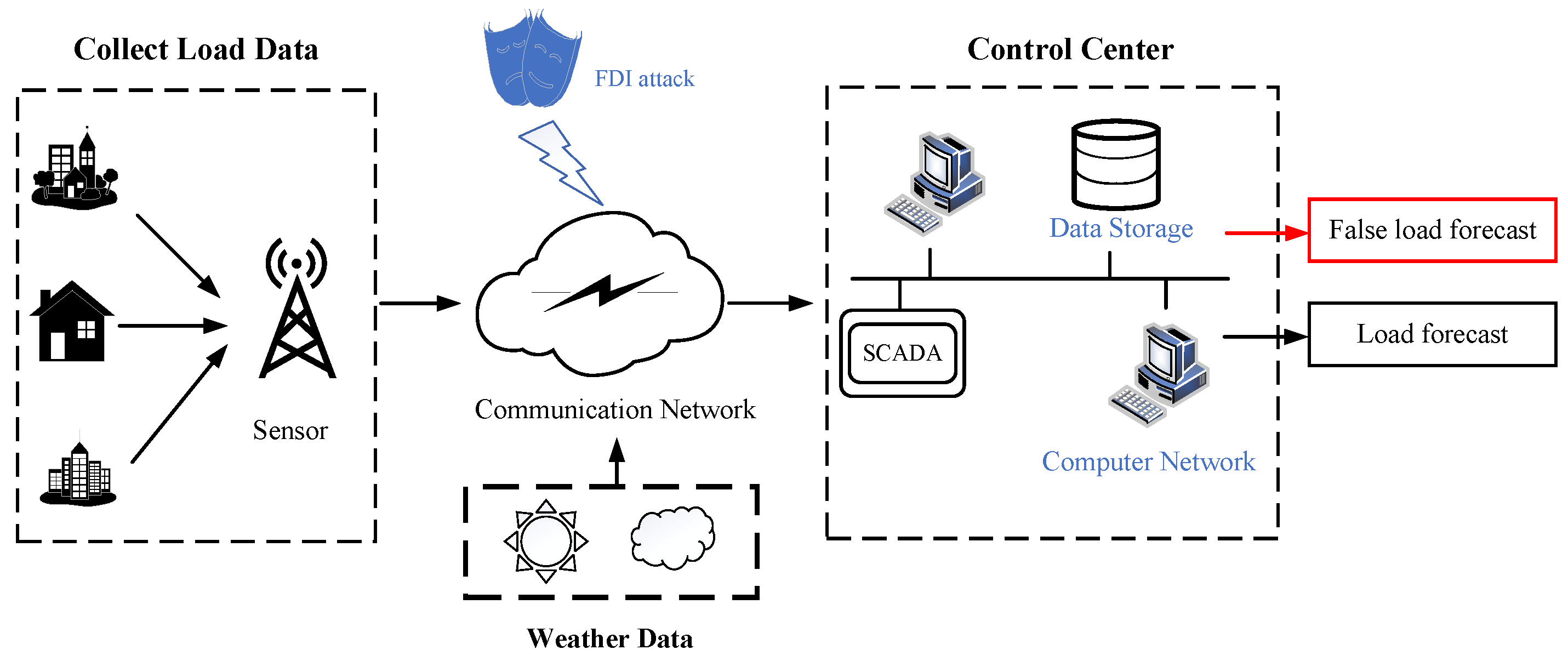
In modern power systems, Transmission System Operators (TSOs) rely on load forecasting outcomes to formulate dispatch plans, thereby ensuring the secure, economical, and stable operation of the grid. Load forecasting systems are typically deployed within control centers, serving as critical decision-support tools for dispatch operations. To produce reliable forecasting results, accurate short-term load forecasting relies on real-time data acquisition with high quality from multiple source nodes. Figure 1 illustrates the typical load forecasting workflow. Sensors first collect electricity consumption data from various nodes, while meteorological data, usually provided by external third-party service providers, are transmitted via communication networks to the control center of the power system. Within the control center, the Supervisory Control and Data Acquisition (SCADA) system consolidates these measurements, which are then stored and fed into forecasting models to generate predictions used in control and dispatch decisions. However, with the increasing interconnection and automation of power systems, cybersecurity threats have become more severe. FDI attacks stand out for their stealth and destructiveness, as attackers can tamper with measurement data during collection or transmission, allowing compromised information to be used in subsequent forecasting and dispatch without detection.

Figure 1. A Process Flow of Load Forecasting.

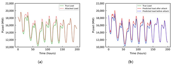
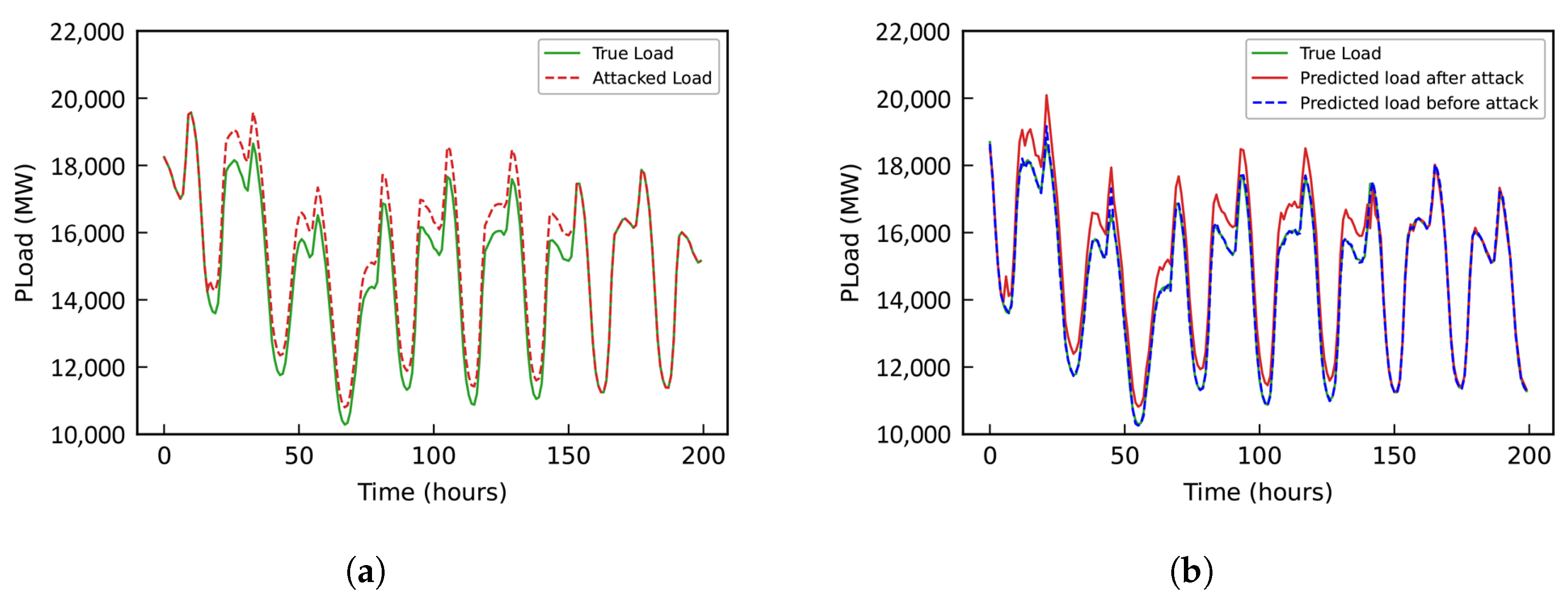
As shown in Figure 2, panel (a) compares the accurate load profile with the perturbed load profile affected by FDI attacks, while panel (b) illustrates the forecasts generated using attacked load data versus those based on clean load data. Directly using load data compromised by FDI attacks for forecasting leads to a significant deviation between the predicted trajectory and the actual load trend, highlighting the detrimental impact of such intrusions on forecasting accuracy. Thus, if the control center directly uses compromised data for forecasting without timely attack detection, the results may deviate significantly from actual load trends, leading to imbalanced generation scheduling, market-clearing errors, and even threats to grid security.

Figure 2. Comparison of Load Profiles and Forecasting Performance Under FDI Attacks. (a) True vs. Perturbed Load Profiles. (b) Forecasts Using Attacked vs. Clean Load Data.

To address this issue, this paper proposes a resilient load forecasting framework based on a collaborative detection and prediction mechanism. The proposed approach enables effective FDI attack detection and data recovery by leveraging only the intrinsic temporal characteristics of the load sequence without relying on any external variables such as weather data. Furthermore, the integration of multi-objective optimization algorithms with multi-model ensemble learning further enhances the robustness of the forecasting. This method offers a practical and scalable solution for enhancing the security and accuracy of load forecasting in innovative grid environments that are vulnerable to cyber threats.

3. FDI Attack Template

In cyber-physical systems (CPS), false data injection attacks on load forecasting sequences $\left\{x_m^A\right\}$ can be formally described as a malicious manipulation process [29].

$${\tilde{x}}_m^A=F(x_m^A,\Theta ),m\in {\mathcal{T}}_a,$$

(1)

where $x_m^A$ denotes the original load data, ${\tilde{x}}_m^A$ represents the tampered data, $F(·)$ represents the attack function, $\Theta$ denotes the attack parameter set, and ${\mathcal{T}}_a$ is the attack duration window indicating the specific moments (m) when the attack is activated.

Based on attacker intentions and strategy differences, we considered four typical attack templates.

3.1. Pulse Attack

The pulse attack injects instantaneous perturbations by manipulating deterministic load values at specific attack moments [30]. The mathematical model is:

$${\tilde{x}}_m^A=(1+{\chi }_P)x_m^A,m=m_p,$$

(2)

where ${\chi }_P$ denotes the pulse intensity factor and $m_p$ represents the occurrence moment of a single pulse attack.

3.2. Scaling Attack

The scaling attack [31] applies proportional scaling to load measurement data during a continuous period ${\mathcal{T}}_a=[m_s,m_e]$, defined as:

$${\tilde{x}}_m^A=(1+{\chi }_S)x_m^A,\forall m\in {\mathcal{T}}_a,$$

(3)

where ${\chi }_S$ represents the scaling factor, with $m_s$ and $m_e$ denoting the start time and end time of a single scaling attack instance, respectively.

3.3. Ramping Attack

The ramping attack [31] is a cyber-physical attack that disrupts normal system operations by gradually tampering with load data. In this study, we focus on the bidirectional ramping attack, which generates a symmetric “hill” pattern with ascending and descending phases, thereby mimicking natural load variations and increasing detection difficulty.

Let $m_s$ and $m_e$ denote the start and end timestamps of the attack interval, respectively, and let $m_c=⌊{\displaystyle \frac{m_s+m_e}{2}}⌋$ be the midpoint. The compromised data are:

$$\begin{array}{cc}\hfill {\tilde{x}}_m^A& =\left[1+{\chi }_R·(m-m_s)\right]x_m^A,m_s<m<m_c,\hfill \\ \hfill {\tilde{x}}_m^A& =\left[1+{\chi }_R·(m_e-m)\right]x_m^A,m_c<m<m_e,\hfill \end{array}$$

(4)

where $x_m^A$ denotes the original load data, ${\chi }_R$ controls the ramp slope, m is the current timestamp within the attack interval, and $\lfloor ·\rfloor$ denotes the floor operation to ensure integer timestamps.

3.4. Random Attack

The random attack [31] injects stochastic perturbations into load measurements by superimposing uniformly distributed noise to degrade system observability and decision-making robustness. The mathematical formulation is defined as:

$${\tilde{x}}_m^A=x_m^A+{\chi }_{RA}·\mathcal{U}\left(m\right),m_s<m<m_e,$$

(5)

where $\mathcal{U}\left(m\right)\sim U(0,1)$ is a uniformly distributed random number generator, ${\chi }_{RA}$ denotes a scaling factor.

4. Methodology

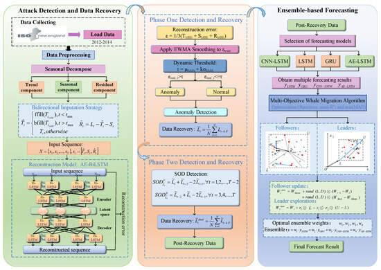
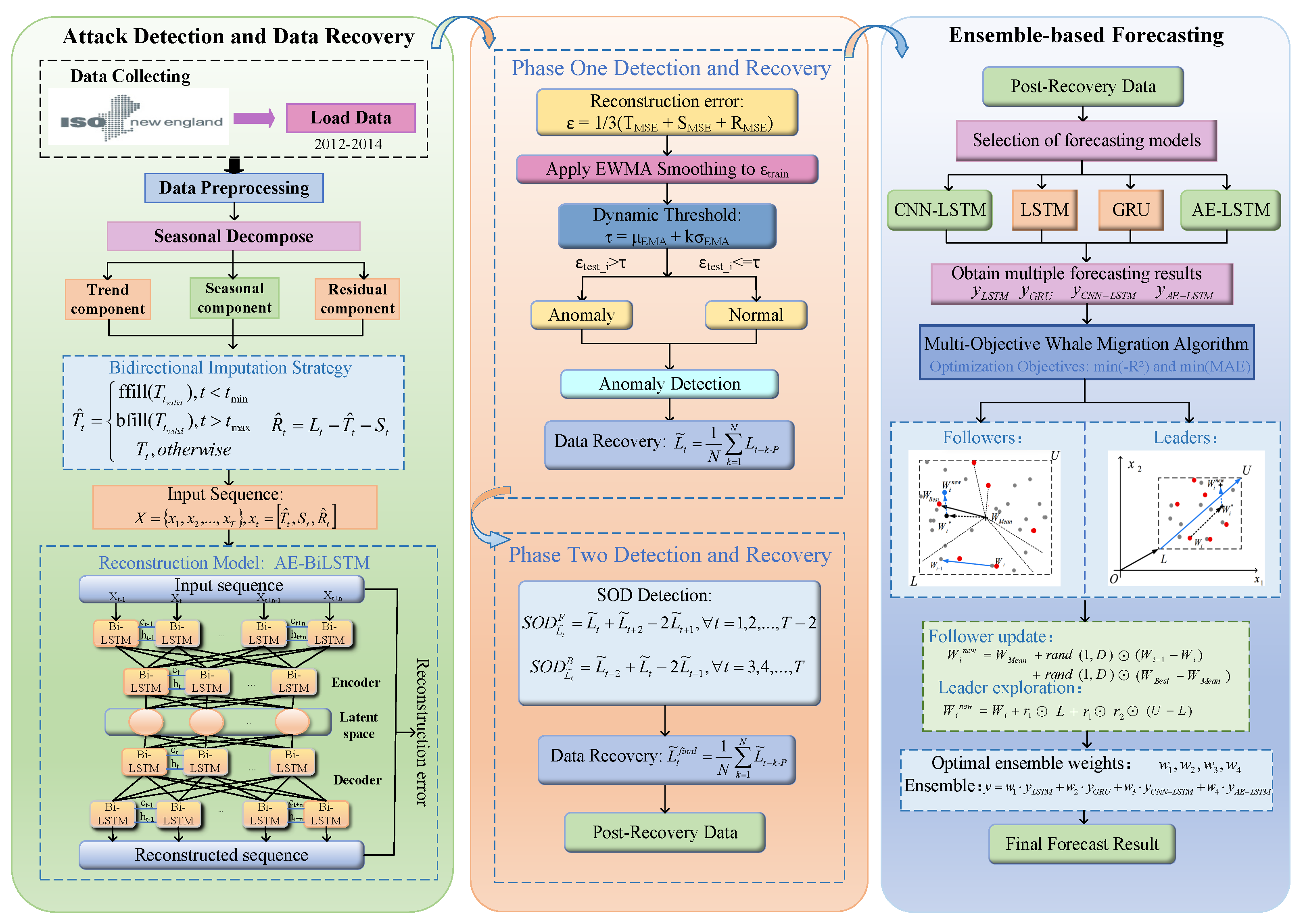
Figure 3 illustrates the proposed detection–prediction collaborative framework. It consists of two closely integrated phases: attack detection and data recovery, and ensemble-based forecasting with multi-objective weighted fusion. First, for attack detection and data recovery, the raw load sequence is decomposed into trend, seasonal, and residual components, and boundary effects are mitigated using bidirectional filling. Each component is then reconstructed using AE-BiLSTM, and the mean of the multi-component reconstruction errors is calculated as an anomaly score. Robust detection is achieved by applying EWMA smoothing to the training set errors and constructing a dynamic threshold. The detected anomalies are recovered using the historical mean at the same time of the week, and a second-order difference (SOD) is applied to further detect and refine the recovered data, thereby enhancing smoothness and reliability. Second, for ensemble-based forecasting, the recovered load data are used as inputs to the prediction models. A hybrid deep learning framework is constructed to achieve accurate load forecasting, and the ensemble parameters are optimized using the MO-WMA algorithm.

Figure 3. Overall Framework Diagram.

4.1. Attack Detection and Recovery

This section describes the proposed attack detection and recovery method. Anomalies are identified through AE-BiLSTM reconstruction with a dynamic threshold, while recovery is achieved via historical mean imputation and Second-Order Difference (SOD) refinement. The resulting cleaned load sequence is smooth, reliable, and serves as high-quality input for subsequent forecasting.

4.1.1. Seasonal Decompose

To address the challenge of detecting stealthy FDI attacks in hourly load measurements without relying on external covariates, we propose a feature-enhanced attack detection framework based on intrinsic temporal pattern decomposition. The raw load data ${\left\{L_t\right\}}_{t=1}^T$ is first decomposed into three interpretable components using seasonal-trend decomposition:

$$L_t=T_t+S_t+R_t,t=1,2,\dots ,N,$$

(6)

where $T_t$, $S_t$, and $R_t$ denote the trend, seasonal, and residual components, respectively, and N represents the total number of observations in the time series. The decomposition is performed via the classical additive model [32] with a moving average window m equal to the seasonal periodicity P (e.g., $P=24$ for daily cycles in hourly data).

Since the centered moving average suffers from boundary effects at the beginning and end of the time series due to incomplete window coverage, a bidirectional imputation strategy is adopted to ensure well-defined trend estimates across the entire sequence.

The trend, seasonal, and residual components are computed as follows:

$$\begin{array}{cc}\hfill T_t& ={\displaystyle \frac{1}{P}}\sum _{k=-\lfloor P/2\rfloor }^{\lfloor P/2\rfloor }{L}_{t+k},\hfill \end{array}$$

(7)

$$\begin{array}{cc}\hfill S_t& ={\displaystyle \frac{1}{n}}\sum _{i=0}^{n-1}(L_{t+iP}-T_{t+iP}),\hfill \end{array}$$

(8)

$$\begin{array}{cc}\hfill R_t& =L_t-T_t-S_t,\hfill \end{array}$$

(9)

where n denotes the number of complete seasonal cycles and k is the symmetric window offset index.

Specifically, the moving average operator in (7) becomes ill-defined for the first and last $\lfloor P/2\rfloor$ observations, introducing boundary artifacts due to incomplete window coverage:

$$\nexists L_{t+k}\mathrm{when}\left\{\begin{array}{cc}t+k<1,\hfill & k\in [-\lfloor P/2\rfloor ,-1]\hfill \\ t+k>N,\hfill & k\in [1,\lfloor P/2\rfloor ].\hfill \end{array}\right.$$

(10)

As a result, trend estimates cannot be directly obtained near the temporal boundaries. To address this issue, a bidirectional imputation strategy is applied, where missing trend values are filled using forward and backward propagation from the nearest valid estimates:

$$\begin{array}{cc}\hfill {\widehat{T}}_t& =\left\{\begin{array}{cc}\mathrm{ffill}\left(T_{t_{\min }}\right),\hfill & t<t_{\min },\hfill \\ \mathrm{bfill}\left(T_{t_{\max }}\right),\hfill & t>t_{\max },\hfill \\ T_t,\hfill & \mathrm{otherwise},\hfill \end{array}\right.\hfill \end{array}$$

(11)

$$\begin{array}{cc}\hfill {\widehat{R}}_t& =L_t-{\widehat{T}}_t-S_t,\hfill \end{array}$$

(12)

where $t_{\min }=\lfloor P/2\rfloor +1$ and $t_{\max }=N-\lfloor P/2\rfloor$ define the valid trend estimation range. Forward-fill (‘ffill’) and backward-fill (‘bfill’) propagate the nearest valid trend estimates to the boundaries, ensuring the entire time series has well-defined trend values.

This decomposition effectively separates the persistent load patterns (trend and seasonal components) from transient anomalies (residual), which allows the subsequent detection stage to focus on identifying FDI attacks within the residual component without interference from long-term or periodic patterns.

4.1.2. AE-BiLSTM Attack Detection and Recovery

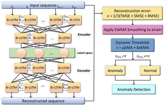
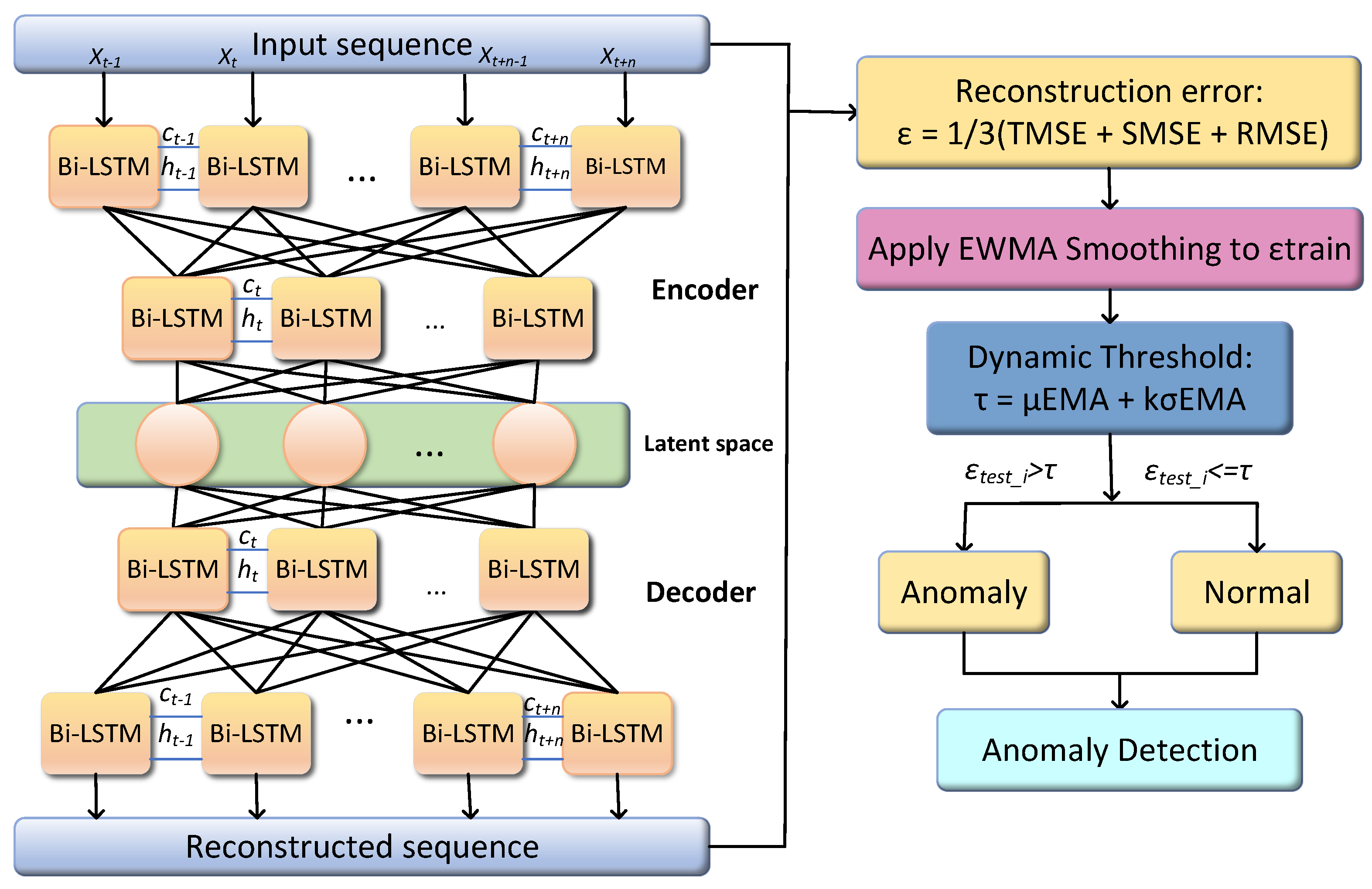
To address the insufficient representation capability of conventional residual-based detection for false data injection attacks, we propose the AE-BiLSTM architecture shown in Figure 4. This framework synergizes the feature reconstruction power of autoencoders with the temporal modeling capacity of BiLSTM networks, enabling coordinated analysis of trend (${\widehat{T}}_t$), seasonal ($S_t$), and residual (${\widehat{R}}_t$) components. Compared to conventional AE-LSTM that employs a unidirectional LSTM for encoding, the AE-BiLSTM captures both past and future temporal dependencies, resulting in a more informative latent representation. The architecture comprises two symmetric modules: a BiLSTM-stacked encoder for cross-component feature extraction and a mirrored BiLSTM decoder for input reconstruction.

Figure 4. AE-BiLSTM Attack Detection Framework.

The raw load data ${\left\{L_t\right\}}_{t=1}^T$ is decomposed into three independent modal components via seasonal decomposition: trend component (${\widehat{T}}_t$), seasonal component ($S_t$), and residual component (${\widehat{R}}_t$). These components provide comprehensive temporal representations, effectively characterizing distinct variation patterns in the sequence. Specifically, the input sequence $\mathbf{X}=\{{\mathbf{x}}_1,{\mathbf{x}}_2,\dots ,{\mathbf{x}}_T\}$ comprises 3D vectors at each timestep t:

$${\mathbf{x}}_t=[{\widehat{T}}_t,S_t,{\widehat{R}}_t]\in {\mathbb{R}}^3,$$

(13)

where ${\widehat{T}}_t$, $S_t$, and ${\widehat{R}}_t$ represent trend, seasonal, and residual features, respectively. This multi-scale modeling facilitates the identification of complex anomaly patterns.

A multi-layer bidirectional LSTM (BiLSTM) network serves as the encoder to process the multi-modal sequence $\mathbf{X}$. By leveraging forward and backward propagation through BiLSTM layers, the model captures bidirectional dependencies and compresses the input sequence into a latent representation $\mathbf{Z}$:

$$\mathbf{Z}={\mathrm{BiLSTM}}_{\mathrm{enc}}(\mathbf{X};{\Theta }_e),$$

(14)

where $\mathbf{X}\in {\mathbb{R}}^{T\times 3}$ denotes the input sequence matrix, ${\Theta }_e$ represents the encoder’s parameter set. The bidirectional architecture enables simultaneous extraction of forward and backward temporal dependencies, enriching contextual information for subsequent decoding.

The decoder reconstructs the original sequence from the latent representation $\mathbf{Z}$ using a mirrored BiLSTM structure:

$$\widehat{\mathbf{X}}={\mathrm{BiLSTM}}_{\mathrm{dec}}(\mathbf{Z};{\Theta }_d),$$

(15)

where ${\Theta }_d$ denotes the decoder’s parameter set.

This learning process minimizes the reconstruction loss error, which measures the difference between the input sequence and its reconstructed output. In our method, to ensure robustness against small anomalies present in the training set, we opt to use the Huber function as the loss function during training [33]:

$${\mathcal{L}}_{\mathrm{Huber}}({\mathbf{x}}_t,{\widehat{\mathbf{x}}}_t)=\left\{\begin{array}{cc}{\displaystyle \frac{1}{2}}{\parallel {\mathbf{x}}_t-{\widehat{\mathbf{x}}}_t\parallel }_2^2,\hfill & \mathrm{if}\parallel {\mathbf{x}}_t-{\widehat{\mathbf{x}}}_t{\parallel }_2\le \delta \hfill \\ \delta \left(\parallel {\mathbf{x}}_t-{\widehat{\mathbf{x}}}_t{\parallel }_2-{\displaystyle \frac{1}{2}}\delta \right),\hfill & \mathrm{otherwise},\hfill \end{array}\right.$$

(16)

where $\delta$ controls the transition threshold between quadratic and linear loss regimes. This hybrid loss function preserves sensitivity to significant deviations while suppressing noise-induced fluctuations.

During training, the AE-BiLSTM model is exposed to regular non-anomalous sequence patterns. It learns to accurately reconstruct these patterns with minimal reconstruction error. Thus, when it encounters an attack, these anomalous patterns deviate from the learned regular patterns and cannot be accurately reconstructed, leading to a noticeable increase in reconstruction error. To compute the reconstruction error, for each sample, we calculate the reconstruction error for its three components: trend ${\widehat{T}}_t$, seasonality $S_t$, and residual ${\widehat{R}}_t$, and take the mean of the reconstruction errors of the three components as the anomaly score for that sample at time t:

$$s_t={\displaystyle \frac{1}{3}}\sum _{k=1}^3{\left(x_t^{\left(k\right)}-{\widehat{x}}_t^{\left(k\right)}\right)}^2,k\in \{{\widehat{T}}_t,S_t,{\widehat{R}}_t\},$$

(17)

where $x_t^{\left({\widehat{T}}_t\right)}$, $x_t^{\left(S_t\right)}$, and $x_t^{\left({\widehat{R}}_t\right)}$ represent the true trend, seasonal, and residual components, respectively.

By setting a threshold for this anomaly score, attacks can be detected. Since load data is often affected by short-term fluctuations and measurement noise when determining the threshold, directly using the raw reconstruction error to set the threshold may lead to a high false positive rate. We apply an exponentially weighted moving average (EWMA) smoothing to the reconstruction errors of the training set, obtaining a smoothed error sequence. EWMA smooths the historical reconstruction errors with weights, thereby diminishing the influence of short-term fluctuations, allowing for a more robust determination of the attack detection threshold. The smoothed error sequence is calculated as:

$${\overline{s}}_t=\lambda s_t^{\left(\mathrm{train}\right)}+(1-\lambda ){\overline{s}}_{t-1},\lambda \in (0,1],$$

(18)

where ${\overline{s}}_t$ represents the smoothed error at timestep t, $s_t^{\left(\mathrm{train}\right)}$ denotes the raw reconstruction error from the training set at timestep t, ${\overline{s}}_{t-1}$ is the smoothed error at the previous timestep $t-1$, and $\lambda$ is the smoothing factor that controls the weighting between historical and current errors. The value of $\lambda$ directly influences the stability of the detection threshold. In this study, the optimal value of $\lambda$ is determined by performing a grid search over $\lambda \in (0,1]$ on a validation set, with performance evaluated using the F1-score and false positive rate.

The dynamic detection threshold is then calculated as:

$$\tau ={\mu }_{\overline{s}}+\kappa {\sigma }_{\overline{s}},$$

(19)

where ${\mu }_{\overline{s}}$ and ${\sigma }_{\overline{s}}$ denote the mean and standard deviation of the smoothed error sequence ${\left\{{\overline{s}}_t\right\}}_{t=1}^T$, $\kappa$ is a constant factor.

For each test sample at timestep t, the computed anomaly score $s_t$ is compared against the dynamic threshold $\tau$ to generate detection alerts:

$${\mathrm{Alert}}_t=\left\{\begin{array}{cc}1,\hfill & \mathrm{if}{s}_t>\tau \hfill \\ 0,\hfill & \mathrm{otherwise},\hfill \end{array}\right.$$

(20)

where ${\mathrm{Alert}}_t=1$ indicates potential FDI attacks or anomalies.

We employ a historical mean recovery strategy for each detected anomalous data point $L_t$ to mitigate the impact of FDI attacks. Leveraging the periodic nature of load data, the anomalous value is replaced by the historical mean of the same time slot from the previous week. This approach effectively smooths out abnormal fluctuations while preserving legitimate temporal patterns.The recovery value ${\tilde{L}}_t$ is computed as:

$${\tilde{L}}_t={\displaystyle \frac{1}{N}}\sum _{k=1}^N{L}_{t-k·P},$$

(21)

where P denotes the period length (e.g., daily period $P=24$ for hourly data), N represents the number of historical cycles (e.g., $N=7$ days for weekly recovery), $L_{t-k·P}$ corresponds to the value at the same time slot in the k-th historical cycle.

4.1.3. SOD Detection and Recovery

After data recovery, although the AE-BiLSTM model has effectively corrected most anomalies, residual anomalies may still exist due to trend variations or short-term fluctuations in the time series. To further refine the data and ensure its smoothness, we introduce the SOD method to identify and correct these potential anomalies.

For the recovered time series ${\left\{{\tilde{L}}_t\right\}}_{t=1}^T$, we compute forward and backward SOD metrics:

$$\begin{array}{cc}\hfill {\mathrm{SOD}}_{{\tilde{L}}_t}^F& ={\tilde{L}}_t+{\tilde{L}}_{t+2}-2{\tilde{L}}_{t+1},\forall t=1,2,\dots ,T-2,\hfill \end{array}$$

(22)

$$\begin{array}{cc}\hfill {\mathrm{SOD}}_{{\tilde{L}}_t}^B& ={\tilde{L}}_{t-2}+{\tilde{L}}_t-2{\tilde{L}}_{t-1},\forall t=3,4,\dots ,T,\hfill \end{array}$$

(23)

where ${\mathrm{SOD}}_{{\tilde{L}}_t}^F$ detects abrupt forward transitions, and ${\mathrm{SOD}}_{{\tilde{L}}_t}^B$ identifies reverse inconsistencies. Persistent anomalies manifest as simultaneous deviations in both directions.

For each timestep t, the composite SOD anomaly score is derived by computing the absolute values of ${\mathrm{SOD}}_{{\tilde{L}}_t}^F$ and ${\mathrm{SOD}}_{{\tilde{L}}_t}^B$ metrics:

$$s_t^{\left(\mathrm{SOD}\right)}=max\left(|{\mathrm{SOD}}_{{\tilde{L}}_t}^F|,|{\mathrm{SOD}}_{{\tilde{L}}_t}^B|\right),$$

(24)

where $s_t^{\left(\mathrm{SOD}\right)}$, the max operator preserves sensitivity to extreme deviations in either temporal direction.

If the anomaly score exceeds the predefined threshold ${\tau }_{\mathrm{SOD}}$, the load data at timestep t is flagged as anomalous. The threshold ${\tau }_{\mathrm{SOD}}$ can be established through offline analysis of historical normal data.

The system first identifies and marks potential anomalies through the following decision rule:

$${\mathrm{Alert}}_t^{\left(\mathrm{SOD}\right)}=\left\{\begin{array}{cc}1,\hfill & \mathrm{if}{s}_t^{\left(\mathrm{SOD}\right)}>{\tau }_{\mathrm{SOD}}\hfill \\ 0,\hfill & \mathrm{otherwise},\hfill \end{array}\right.$$

(25)

where ${\mathrm{Alert}}_t^{\left(\mathrm{SOD}\right)}=1$ indicates an anomalous data point at timestep t. For each marked anomaly (${\mathrm{Alert}}_t^{\left(\mathrm{SOD}\right)}=1$), we implement the historical mean recovery strategy as described in Section 4.1.2, resulting in the final recovered data ${\left\{{\tilde{L}}_t^{\mathrm{final}}\right\}}_{t=1}^T$. By introducing the SOD method, we can further capture and correct residual anomalies that are difficult to detect through reconstruction errors, thereby improving the smoothness of the data and ensuring more reliable input for load forecasting.

The detailed steps of the entire process are illustrated in Algorithm 1.

Algorithm 1 Detection and Recovery of Load Sequence

1: Input: Raw load sequence ${\left\{L_t\right\}}_{t=1}^T$ 2: Output: Final recovered load sequence ${\left\{{\tilde{\mathbf{L}}}_t^{\mathrm{final}}\right\}}_{t=1}^T$ 3: Stage 1: Seasonal Decomposition & AE-BiLSTM Detection 4: Decompose ${\left\{L_t\right\}}_{t=1}^T$ into trend ${\widehat{T}}_t$, seasonal $S_t$, and residual ${\widehat{R}}_t$ 5: Mitigate boundary effects using forward/backward filling 6: Construct input sequence $\mathbf{X}=\{{\mathbf{x}}_1,{\mathbf{x}}_2,\dots ,{\mathbf{x}}_T\}$, ${\mathbf{x}}_t=[{\widehat{T}}_t,S_t,{\widehat{R}}_t]\in {\mathbb{R}}^3$ 7: for  $t=1,\dots ,T$  do 8:        Reconstruct $\widehat{\mathbf{X}}$ using AE-BiLSTM 9:        Compute reconstruction aggregate error for each component: $s_t={\displaystyle \frac{1}{3}}{\sum }_{k=1}^3{\left(x_t^{\left(k\right)}-{\widehat{x}}_t^{\left(k\right)}\right)}^2$, $k\in \{{\widehat{T}}_t,S_t,{\widehat{R}}_t\}$ 10: end for 11: Apply EWMA smoothing to $\left\{s_t\right\}$ and compute dynamic threshold: $\tau ={\mu }_{\overline{s}}+\kappa {\sigma }_{\overline{s}}$ 12: Mark time t as anomalous if $s_t>\tau$ 13: Replace anomalies with historical mean at the same weekly time slot: ${\tilde{L}}_t={\displaystyle \frac{1}{N}}{\sum }_{k=1}^N{L}_{t-k·P}$ 14: Stage 2: Second-Order Difference (SOD) Refinement 15: for  $t=1,2,\dots ,T$  do 16:     Compute forward and backward SOD: $${\mathrm{SOD}}_{{\tilde{L}}_t}^F={\tilde{L}}_{t+2}-2{\tilde{L}}_{t+1}+{\tilde{L}}_t,\forall t=1,2,\dots ,T-2$$ $${\mathrm{SOD}}_{{\tilde{L}}_t}^B={\tilde{L}}_{t-2}+{\tilde{L}}_t-2{\tilde{L}}_{t-1},\forall t=3,4,\dots ,T$$ 17:     Composite SOD score: $s_t^{\left(\mathrm{SOD}\right)}=max\left(|{\mathrm{SOD}}_{{\tilde{L}}_t}^F|,|{\mathrm{SOD}}_{{\tilde{L}}_t}^B|\right)$ 18:     if $s_t^{\left(\mathrm{SOD}\right)}>{\tau }_{\mathrm{SOD}}$ then 19:         Replace ${\tilde{L}}_t$ with historical mean at the same weekly time slot 20:     end if 21: end for 22: Return: Final recovered load sequence ${\left\{{\tilde{L}}_t^{\mathrm{final}}\right\}}_{t=1}^T$

4.2. Multi-Objective Optimization-Based Ensemble Forecasting

After completing the attack detection and data recovery using AE-BiLSTM and SOD, this study develops an ensemble forecasting framework to enhance load forecasting performance. The framework takes the recovered load data sequence $\tilde{L}{t}^{\mathrm{final}}{t=1}^T$ as unified input and integrates four base predictors: Long Short-Term Memory (LSTM) [34,35], Gated Recurrent Unit (GRU) [36], Autoencoder-LSTM (AE-LSTM), and CNN-LSTM networks. These models are selected for their complementary strengths in capturing different temporal and feature characteristics of load data. Specifically, LSTM networks are effective in modeling long-term dependencies, while GRU efficiently represents medium- and short-term patterns. The CNN-LSTM model captures local spatiotemporal structures, such as daily load cycles, through convolutional layers. Additionally, the AE-LSTM enhances robustness against noise and anomalies by leveraging autoencoder-based feature extraction. By employing multi-objective weight optimization, the proposed framework achieves significant improvements in both prediction accuracy and robustness.

4.2.1. Multi-Objective Whale Migration Algorithm

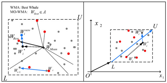
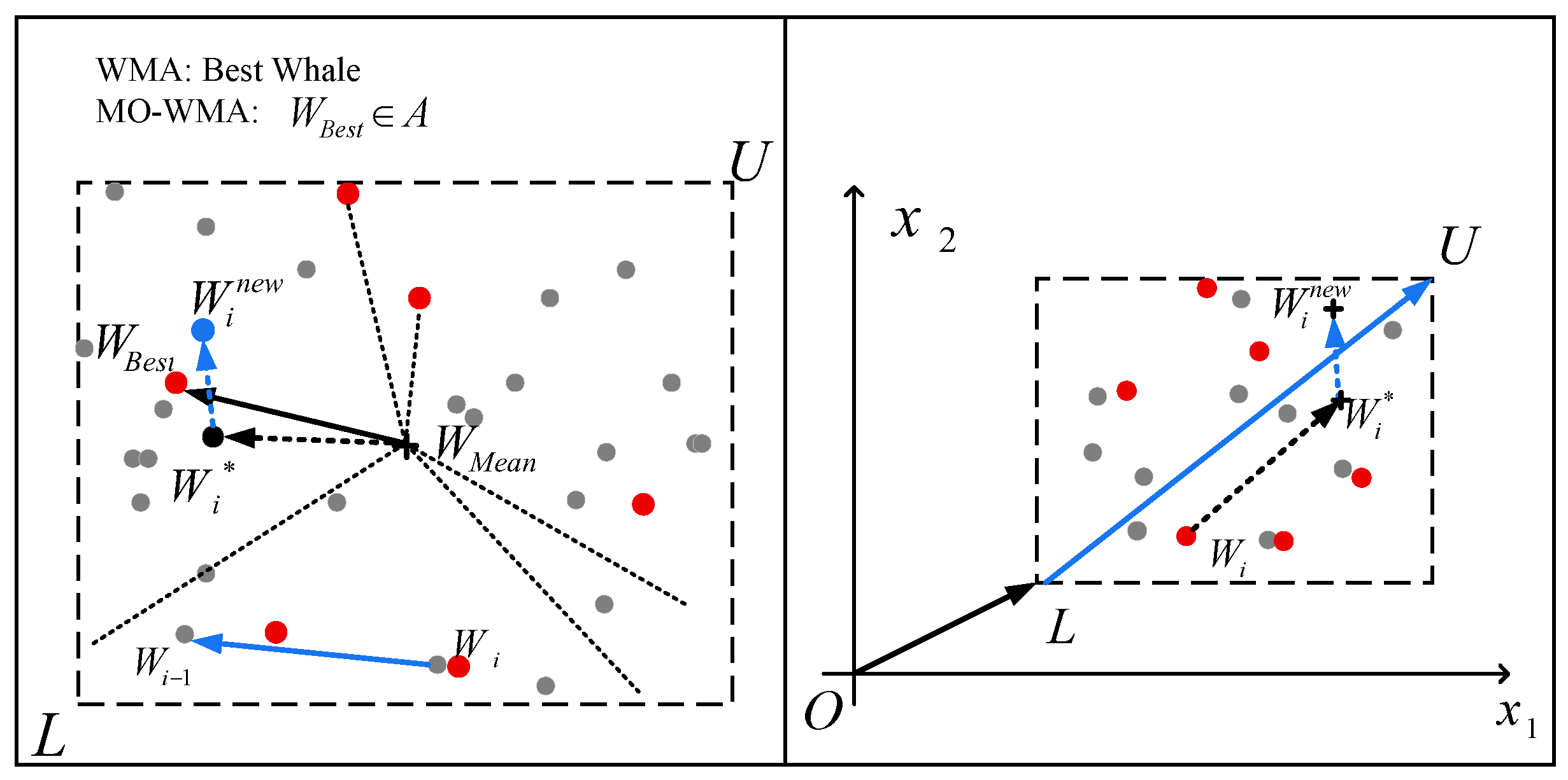
The Whale Migration Algorithm (WMA) is a population-based metaheuristic inspired by the long-distance migratory behavior of humpback whales (Megaptera novaeangliae) [37]. By simulating the cooperative interactions between leader whales and follower whales, WMA achieves a dynamic balance between global exploration and local exploitation. Figure 5 illustrate the movement patterns of the followers (left) and leaders (right) whales. However, the original design of WMA is tailored for single-objective optimization problems and cannot simultaneously handle multiple conflicting objectives. To address this limitation, this study proposes the Multi-Objective Whale Migration Algorithm (MO-WMA), which extends the WMA framework by incorporating non-dominated sorting, crowding distance, and an external archive mechanism. These enhancements enable MO-WMA to search for the Pareto-optimal set in multi-objective optimization problems effectively.

Figure 5. Schematic Illustration of the Movements of Followers (Left) and Leaders (Right).

By combining the global search capability of the Whale Migration Algorithm (WMA) with the Pareto dominance principle from multi-objective optimization, MO-WMA ensures convergence while maintaining solution diversity, thereby generating well-distributed Pareto front approximations in a single run. Compared to the classical NSGA-II, MO-WMA adopts its non-dominated sorting and crowding distance mechanisms, but replaces genetic operations with a whale-migration-inspired search strategy, enabling a more natural balance between exploration and exploitation with lower computational overhead, which is particularly suitable for real-time optimization of ensemble weights in load forecasting models.

Improvement 1: Non-Dominated Sorting

MO-WMA employs the non-dominated sorting procedure from NSGA-II to rank individuals based on dominance relations. For two solutions p and q, if

$$\forall k,f_k\left(p\right)\le f_k\left(q\right)\mathrm{and}\exists k,f_k\left(p\right)<f_k\left(q\right),$$

(26)

then p dominates q, where $f_k(·)$ denotes the k-th objective function value. After sorting, the first Pareto front $F_1$ contains all non-dominated solutions in the population.

Improvement 2: Crowding Distance

To maintain diversity in the Pareto front, MO-WMA calculates the crowding distance $C{D}_i$ for each solution i in the front $F_j$. The crowding distance on objective m is computed as

$$C{D}_i^m={\displaystyle \frac{f_m(i+1)-f_m(i-1)}{f_m^{max}-f_m^{min}}},$$

(27)

where $f_m(i+1)$ and $f_m(i-1)$ are the objective values of the immediate neighbors of solution i in the sorted list for objective m, and $f_m^{max}$, $f_m^{min}$ are the maximum and minimum objective values in $F_j$, respectively. The total crowding distance for solution i is the sum over all objectives:

$$C{D}_i=\sum _{m=1}^{M}C{D}_i^m.$$

(28)

Improvement 3: External Archive Mechanism

MO-WMA maintains an external archive A to store all non-dominated solutions found during the search. After each iteration, the archive is updated by merging with the current non-dominated front $F_1$:

$$A\leftarrow A\cup F_1.$$

(29)

Dominated solutions in A are removed. If the archive size exceeds the maximum capacity $N_A$, solutions are sorted by ascending crowding distance $C{D}_i$, and solutions with the smallest crowding distances are removed to maintain diversity.

4.2.2. MO-WMA for Ensemble Forecasting

The overall framework of MO-WMA preserves the fundamental structure of WMA while incorporating multi-objective optimization mechanisms into the leader selection and individual update strategies. This study applies the MO-WMA to the ensemble weight optimization problem in load forecasting, aiming to automatically search for the optimal weight vector $\mathbf{w}=[w_1,w_2,w_3,w_4]$ to achieve an optimal fusion of predictions from four base models (LSTM, GRU, CNN-LSTM, and AE-LSTM).

Specifically, MO-WMA adopts two complementary objective functions as optimization criteria:

• $f_1\left(\mathbf{w}\right)$: Minimization of the Mean Absolute Error (MAE), which measures the average deviation between predicted and actual values. Compared with Mean Squared Error (MSE) and Root Mean Squared Error (RMSE), MAE is more robust to outliers and provides a more stable evaluation of overall prediction error. Compared to Mean Absolute Percentage Error (MAPE), MAE avoids error inflation when actual values approach zero, making it more practical and reliable in load forecasting contexts.
• $f_2\left(\mathbf{w}\right)$: Minimization of the negative coefficient of determination ($-R^2$), i.e., maximization of $R^2$, which reflects the model’s ability to capture the trend of load variations. Unlike pure error metrics, $R^2$ emphasizes how well the predictions align with the overall time series trend, ensuring that the model not only achieves numerical accuracy but also effectively captures load dynamics.

The choice to optimize MAE and $R^2$ separately, rather than combining them into a single objective, is motivated by the inherent trade-off between these metrics. Simple linear weighting schemes require subjective weight assignment, which may bias optimization towards one metric at the expense of the other. Multi-objective optimization enables simultaneous consideration of prediction accuracy and trend fitting, exploring a Pareto-optimal set that balances these two aspects, thereby enhancing the scientific rigor and flexibility of weight selection.

In summary, by jointly optimizing MAE and $R^2$, MO-WMA effectively obtains a set of weight solutions that achieve a favorable trade-off between prediction accuracy and trend adherence. The detailed procedure is described as follows:

Step 1: Initialization

A population of $N_{pop}$ whale individuals is randomly initialized within the search space. Each ${\mathbf{W}}_i$ represents a candidate weight vector of dimension D (in this study, $D=4$), corresponding to the fusion coefficients for the ensemble prediction models.

The components of each weight vector are uniformly sampled from a bounded interval (e.g., $[0.1,0.9]$):

$${\mathbf{W}}_i=\mathbf{L}+\mathrm{rand}(1,D)\odot (\mathbf{U}-\mathbf{L}),i=1,2,\dots ,N_{pop},$$

(30)

where $\mathbf{L}$ and $\mathbf{U}$ denote the lower and upper bounds of the search space, and ⊙ denotes the Hadamard (element-wise) product.

To ensure the weights are meaningful for ensemble prediction, each vector is normalized before fitness evaluation:

$$w_j^{\mathrm{norm}}={\displaystyle \frac{w_j}{{\sum }_{k=1}^D{w}_k}},j=1,2,\dots ,D.$$

(31)

The ensemble prediction for each individual is computed using the normalized weight vector, and the multi-objective fitness is evaluated based on the mean absolute error (MAE) and the negative coefficient of determination ($-R^2$):

$$\mathbf{F}\left({\mathbf{W}}_i\right)=[f_1\left({\mathbf{W}}_i\right),f_2\left({\mathbf{W}}_i\right)]=[-R^2,\mathrm{MAE}].$$

(32)

The population is then sorted using non-dominated sorting, and the first Pareto front $F_1$ is identified. An external archive A is initialized to store all non-dominated solutions:

$$A\leftarrow F_1,$$

(33)

where A maintains a maximum size of $N_A$ and is updated throughout the optimization process to preserve diversity among solutions.

Step 2: Leader Selection

The top $N_L$ whales from the first Pareto front $F_1$ are selected as leaders based on their crowding distance and dominance rank. The mean position of these leaders ${\mathbf{W}}_{Mean}$ is computed as:

$${\mathbf{W}}_{Mean}={\displaystyle \frac{1}{N_L}}\sum _{j=1}^{N_L}{\mathbf{W}}_j.$$

(34)

This center serves as a reference for guiding the movement of followers.

Step 3: Follower Update

The remaining whales $(i=N_L+1,\dots ,N_{pop})$ update their positions by learning from their immediate superior and the leaders’ mean position:

$$\begin{array}{cc}\hfill {\mathbf{W}}_i^{new}={\mathbf{W}}_{Mean}& +\mathrm{rand}(1,D)\odot ({\mathbf{W}}_{i-1}-{\mathbf{W}}_i)\hfill \\ \hfill & +\mathrm{rand}(1,D)\odot ({\mathbf{W}}_{Best}-{\mathbf{W}}_{Mean}),\hfill \end{array}$$

(35)

where ${\mathbf{W}}_{Best}$ is randomly selected from the archive A. If ${\mathbf{W}}_i^{new}$ dominates ${\mathbf{W}}_i$, or improves diversity (evaluated by crowding distance), the update is accepted.

Step 4: Leader Exploration

Leaders explore the search space using a global exploration strategy:

$${\mathbf{W}}_i^{new}={\mathbf{W}}_i+r_1\odot \mathbf{L}+r_1\odot r_2\odot (\mathbf{U}-\mathbf{L}),$$

(36)

where $r_1$, $r_2\in [0,1]$ are random vectors, and $\mathbf{L},\mathbf{U}$ are lower and upper bounds of the search space. Updates are retained if the new solution belongs to a better Pareto front or increases diversity in A.

Step 5: Archive Update and Termination

At the end of each iteration, the archive A is updated:

$$A\leftarrow A\cup F_1.$$

(37)

Dominated solutions in A are removed. If $\left|A\right|>N_A$, solutions with the smallest crowding distances are eliminated to preserve diversity. The algorithm terminates when the maximum number of iterations is reached or a satisfactory Pareto front approximation is achieved.

The detailed steps are summarized in Algorithm 2.

Algorithm 2 MO-WMA Algorithm

1: Input: Maximum iterations $Ite{r}_{max}$, population size $N_{pop}$, number of leaders $N_L$, archive size $N_A$, bounds $\mathbf{L}$ and $\mathbf{U}$ 2: Initialize population: ${\mathbf{W}}_i=\mathbf{L}+\mathrm{rand}\odot (\mathbf{U}-\mathbf{L}),i=1,\dots ,N_{pop}$ Normalize each ${\mathbf{W}}_i$ so that ${\sum }_{j=1}^D{w}_{ij}=1$ 3: Evaluate the multi-objective fitness $\mathbf{F}\left({\mathbf{W}}_i\right)=[-R^2,\mathrm{MAE}]$ for each whale and perform non-dominated sorting; initialize archive $A\leftarrow F_1$ 4: for iteration = 1 to $Ite{r}_{max}$ do 5:      Select top $N_L$ leaders from the first Pareto front $F_1$; compute leader mean position ${\mathbf{W}}_{Mean}$ 6:      for $i=N_L+1$ to $N_{pop}$ do                    ▹ Follower update 7:         Randomly select ${\mathbf{W}}_{Best}$ from archive A 8:         Update position: $${\mathbf{W}}_i^{new}={\mathbf{W}}_{Mean}+\mathrm{rand}\odot ({\mathbf{W}}_{i-1}-{\mathbf{W}}_i)+\mathrm{rand}\odot ({\mathbf{W}}_{Best}-{\mathbf{W}}_{Mean})$$ 9:         Accept ${\mathbf{W}}_i^{new}$ if it dominates ${\mathbf{W}}_i$ or improves diversity 10:    end for 11:    for $i=1$ to $N_L$ do                    ▹ Leader exploration 12:        Generate new position via global exploration 13:        Accept new position if it improves Pareto dominance or diversity in A 14:    end for 15:    Re-evaluate population, perform non-dominated sorting, update archive $A\leftarrow A\cup F_1$ 16:    If $\left|A\right|>N_A$, prune archive by removing solutions with smallest crowding distances 17: end for 18: Output: Non-dominated archive A

The final output is a set of non-dominated weight vectors $\mathbf{w}$. From these, the best trade-off solution is selected and substituted into the weighted ensemble formula to generate the final load forecast:

$$Y=w_1{y}_{\mathrm{LSTM}}+w_2{y}_{\mathrm{GRU}}+w_3{y}_{\mathrm{CNN}-\mathrm{LSTM}}+w_4{y}_{\mathrm{AE}-\mathrm{LSTM}}.$$

(38)

This strategy enables the ensemble model to enhance prediction accuracy while maintaining effective fitting of the load variation trend, thereby improving the overall robustness and practical value of the model.

5. Experiments

5.1. Data and Attack Configuration

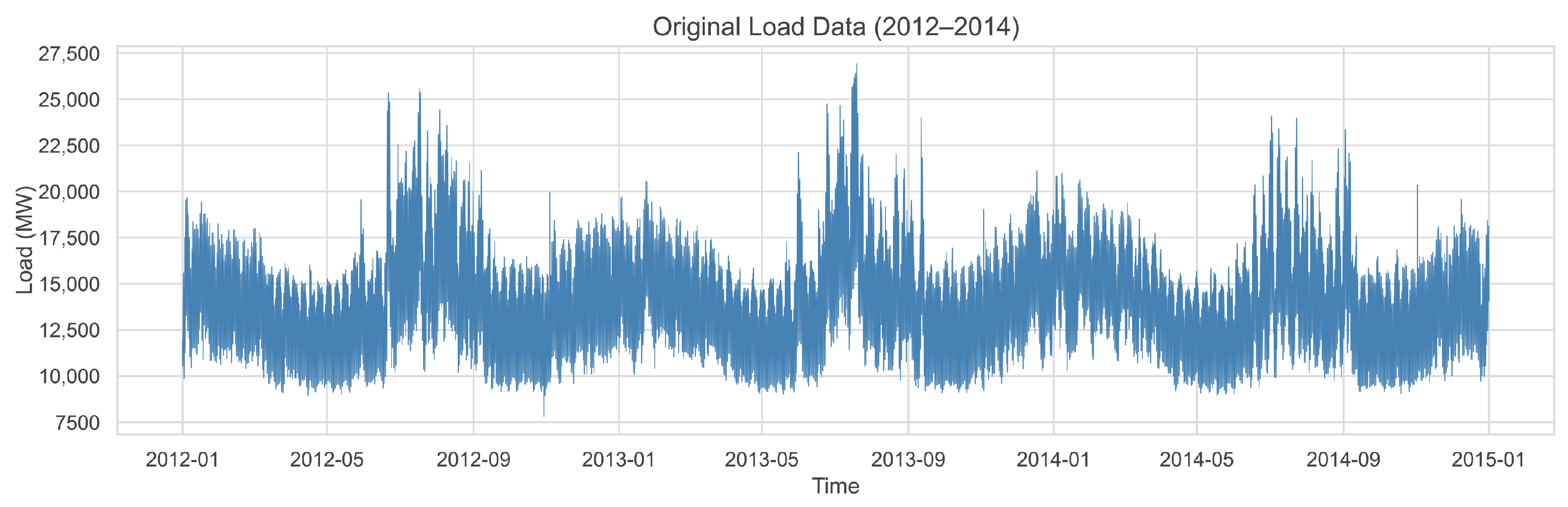
The proposed two-stage anomaly detection framework is validated against FDI attacks using hourly load data from ISO New England (2012–2014). As illustrated in Figure 6, the 2012–2013 datasets, which contain only normal, attack-free load records, are used to train the models. The 2014 dataset (8760 samples) serves as the test set with four FDIA types injected: Scaling, Ramping, Pulse, and Random attacks, whose parameter configurations are detailed in Table 2.

Figure 6. Original Load Distribution.

Table 2. Attack Parameter Settings.

Attack Type	Parameter Value	Attack Period
Scaling Attack	${\chi }_S=0.5$	01-13 01:00 to 01-14 15:00
Ramping Attack	${\chi }_R=0.021$	03-13 00:00 to 03-15 23:00
Random Attack	${\chi }_{RA}=max\left(L_m^A\right)/2.8$	05-01 01:00 to 05-01 20:00
Scaling Attack	${\chi }_S=0.3$	07-13 15:00 to 07-15 15:00
Pulse Attack	${\chi }_P=0.5$	10-01 and 10-02 06:00
Pulse Attack	${\chi }_P=0.4$	12-03 and 12-04 08:00

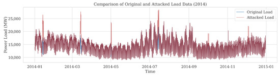
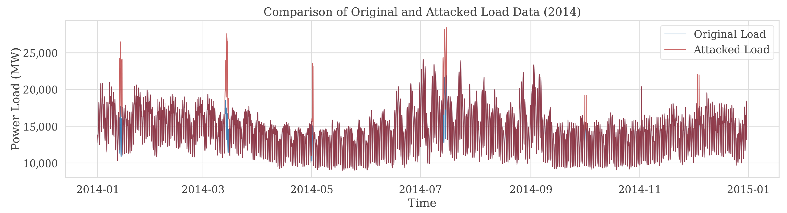
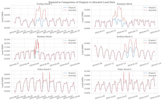
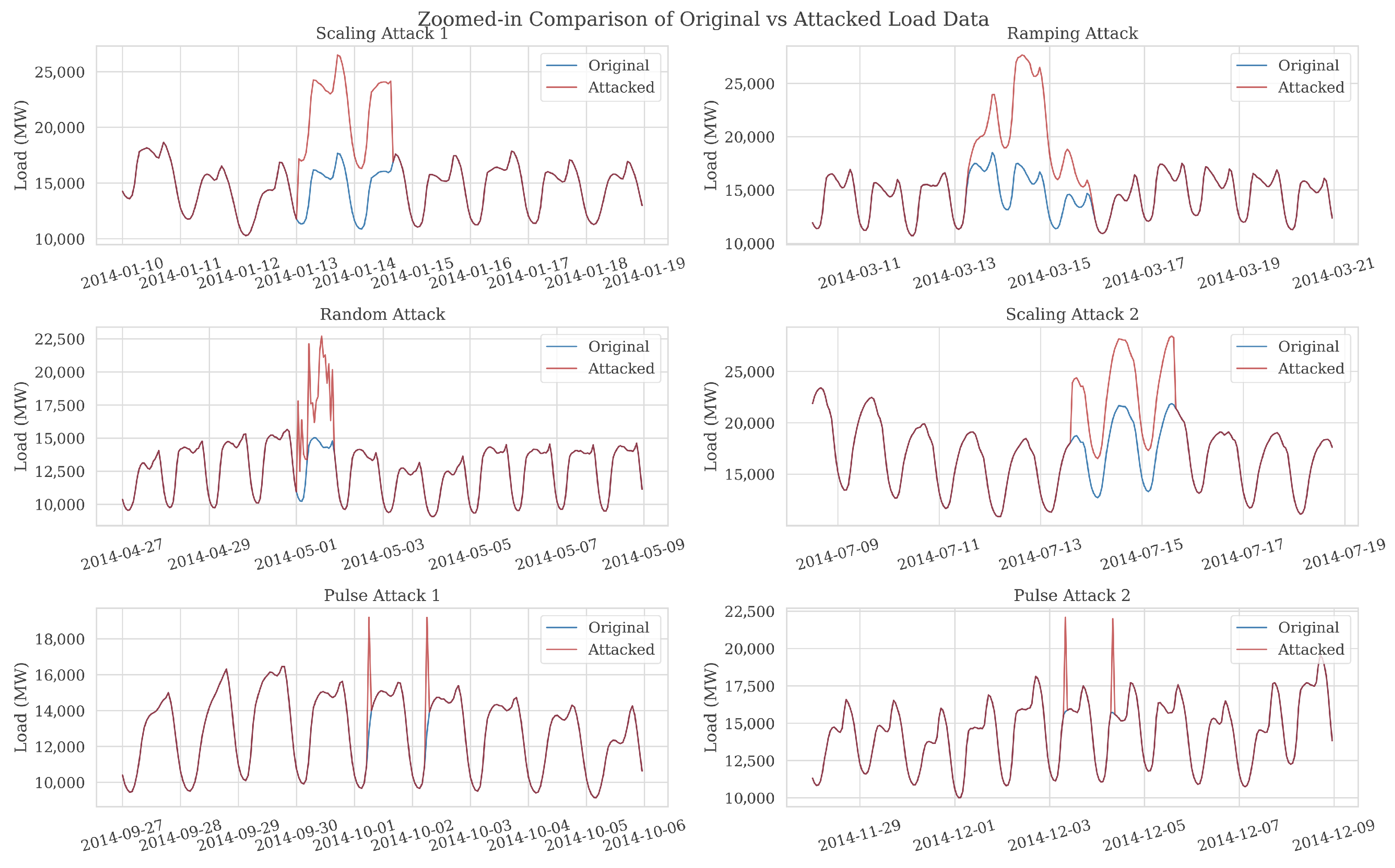
The attack parameters are determined according to the pronounced diurnal and seasonal characteristics of the ISO-NE load data, to balance attack stealthiness and effectiveness. Moderate-amplitude perturbations are adopted to ensure that the injected attacks can induce noticeable deviations in the load profile and degrade forecasting performance, while remaining partially concealed within natural load fluctuations. All attacks are implemented over limited temporal intervals rather than the entire load series, further enhancing the realism of the experimental setup. Temporal comparisons between the original and compromised data, with local magnified views, are shown in Figure 7 and Figure 8. Subsequently, both the training and test datasets were normalized using min-max scaling to ensure consistent feature representation across all datasets.

Figure 7. Comparison of Original and Attacked Load Data (2014).

Figure 8. Comparison of Original and Attacked Load Data.

5.2. Performance Evaluation of Attack Detection

5.2.1. Results and Analysis of Attack Detection

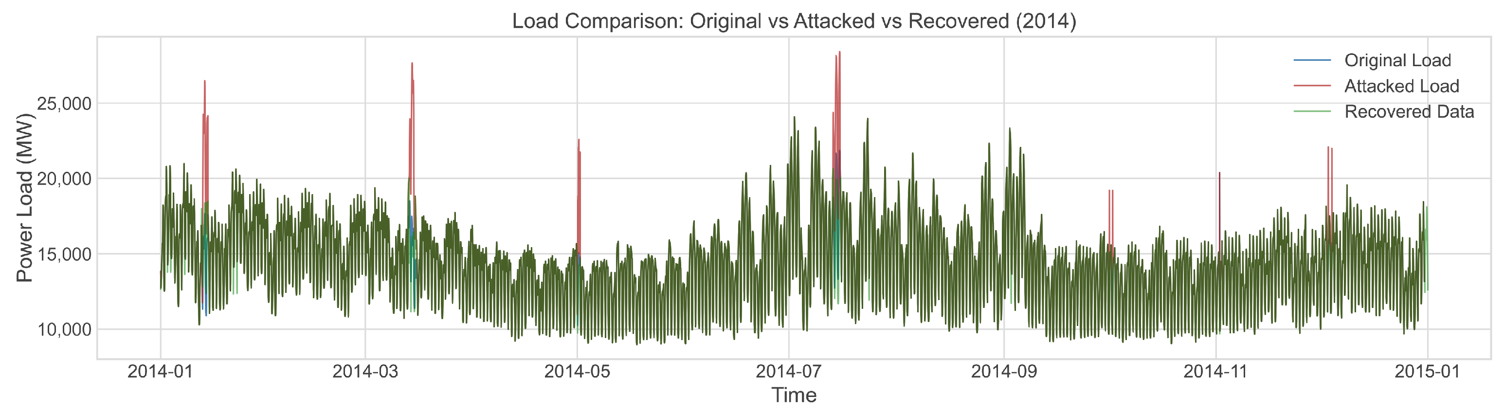
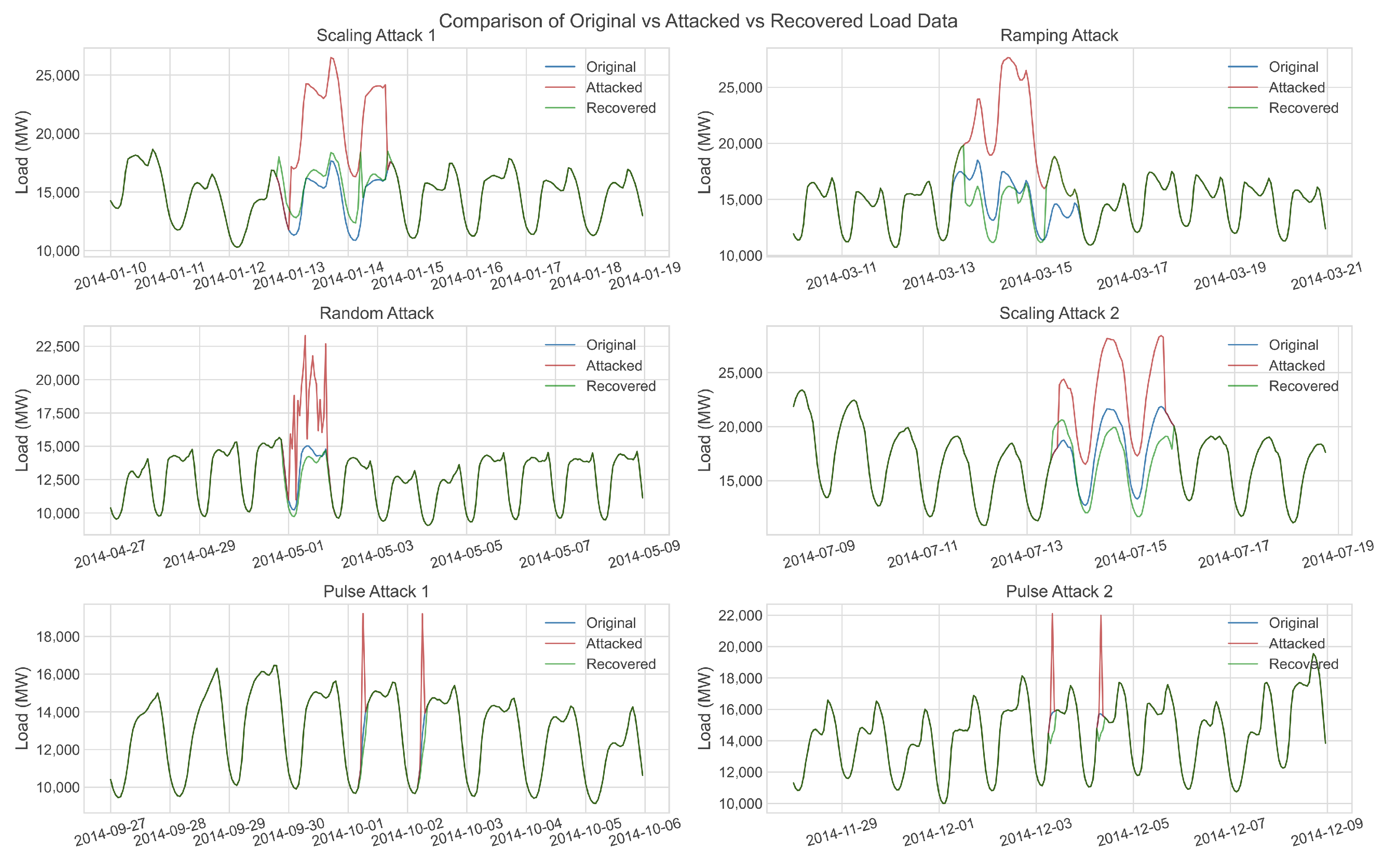
As illustrated in Figure 7 and Figure 8, the load data exhibit significant fluctuations, and certain types of attacks, such as ramping attacks, are visually similar to natural load variations. This poses a substantial challenge for anomaly detection. This study uses only historical load data to train the models for detecting various types of FDI attacks. To comprehensively evaluate the detection performance of the proposed two-stage framework, multiple FDIA types are injected into the 2014 dataset.

To validate the efficacy of the proposed AE-BiLSTM-SOD framework, four state-of-the-art unsupervised models are adopted as benchmarks: Autoencoder (AE), AE-LSTM, Variational Autoencoder LSTM (VAE-LSTM), and Deep Autoencoding Gaussian Mixture Model (DAGMM) [38]. All models are trained on the 2012–2013 dataset with manual hyperparameter optimization. The proposed model employs a three-channel input architecture (trend, seasonal, and residual components) with a 24-h temporal window. Key hyperparameter configurations are detailed in Table 3. In the comparative evaluation, six primary evaluation metrics were utilized for assessment.

$$\begin{array}{cc}\hfill & Accuracy=(\mathrm{TP}+\mathrm{TN})/(\mathrm{TP}+\mathrm{TN}+\mathrm{FP}+\mathrm{FN})\hfill \end{array}$$

(39)

$$\begin{array}{cc}\hfill & Precision=\mathrm{TP}/(\mathrm{TP}+\mathrm{FP})\hfill \end{array}$$

(40)

$$\begin{array}{cc}\hfill & Recall=\mathrm{TP}/(\mathrm{TP}+\mathrm{FN})\hfill \end{array}$$

(41)

$$\begin{array}{cc}\hfill & F1score=2\mathrm{TP}/(2\mathrm{TP}+\mathrm{FP}+\mathrm{FN})\hfill \end{array}$$

(42)

$$\begin{array}{cc}\hfill & FPR=\mathrm{FP}/(\mathrm{FP}+\mathrm{TN}),\hfill \end{array}$$

(43)

where TP represents correctly identified attacks, FP represents incorrectly identified attacks, TN represents correctly identified benign data points, and FN represents incorrectly identified benign data points. Accuracy measures the overall accuracy of the model. Precision reflects the accuracy of attack identification results. Recall (i.e., sensitivity) illustrates the capability of the model to comprehend the various scenarios of FDI attacks. The F1-score denotes the general model’s precision, where a high F1-score implies few FP and FN. False Positive Rate (FPR) evaluates the classification error ratio of misidentifying normal data points as attacks. ROC AUC (Area Under the Receiver Operating Characteristic Curve) quantifies the model’s ability to distinguish between normal data and attacks. The outcomes of these evaluation metrics across diverse classification models are demonstrated in Table 4.

Table 3. Hyperparameter Configuration.

Parameter	Value
BiLSTM Layer Structure	[128, 64, 32]
Latent Dimension	64
Learning Rate	0.001
Batch Size	32

Table 4. FDI Attack Detection Performance of Different Models (%).

Model	Accuracy	Precision	Recall	F1	FPR	ROC AUC
AE	97.97	50.25	55.31	52.66	1.14	77.08
AE-LSTM	98.52	64.50	60.89	62.64	0.70	80.10
VAE-LSTM	98.33	60.12	54.75	57.31	0.76	77.00
DAGMM	97.99	50.89	48.04	49.43	0.97	73.50
Proposed	98.98	71.23	84.36	77.24	0.71	91.82

As demonstrated in Table 4, the proposed method exhibits significant improvements across all evaluation metrics, highlighting its effectiveness in detecting FDI attacks in load data. The proposed model outperforms benchmark models substantially in both recall (0.8436) and ROC AUC (0.9182). Specifically, compared with AE-LSTM, our method achieves a $23.5\%$ higher recall rate while maintaining a comparable FPR ($0.71\%$ vs. $0.70\%$), indicating enhanced capability to identify stealthy attacks (e.g., ramp attacks) and reduced misclassification of normal load fluctuations. The ROC AUC comparison further reveals superior detection sensitivity in low false favorable rate regimes (FPR $<0.01$) compared with other models.

5.2.2. Ablation Study of Attack Detection

To validate the contributions of individual components in the proposed attack detection framework, we conducted ablation studies to analyze the effects of seasonal decomposition, SOD secondary detection, and EWMA smoothing. As demonstrated in Table 5, removing seasonal decomposition caused a $19.7\%$ decrease in recall for ramp attacks (from 0.8436 to 0.6480) and a 0.09 reduction in ROC AUC, indicating that the seasonal decomposition strategy effectively captures multi-scale anomalous features induced by attacks through the separation of trend and residual components. The removal of SOD secondary detection led to a $0.1\%$ increase in false positive rate (FPR: from 0.0071 to 0.0079) coupled with a $14.2\%$ rise in false negative rate (FNR: from 0.1564 to 0.2961), evidencing its capability to filter out false anomalies from single-stage detection. Furthermore, EWMA smoothing reduced FNR by an additional $5.9\%$ (from 0.2123 to 0.1564 without smoothing), highlighting its critical role in enhancing model robustness by suppressing high-frequency noise in residual components.

Table 5. Ablation Analysis (%).

Variant	Accuracy	Precision	Recall	F1	FPR	ROC AUC
w/o Decompose	98.61	66.29	64.80	65.54	0.69	82.06
w/o SOD	98.80	70.79	70.39	70.59	0.61	84.61
w/o EWMA	99.11	77.90	78.77	78.33	0.47	89.15
Full Model	98.98	71.23	84.36	77.24	0.71	91.82

5.2.3. Data Recovery Results

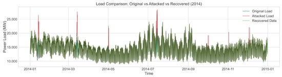
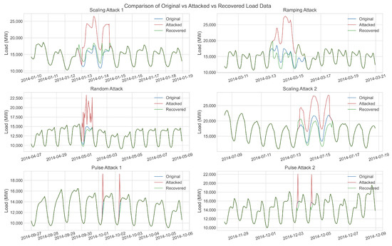
In power load forecasting tasks, input data’s integrity critically determines models’ predictive reliability. This study develops a multi-phase restoration strategy integrating temporal periodicity characteristics to mitigate data distortion caused by FDI attacks. First, a two-stage anomaly detection framework precisely localizes compromised data points. Subsequently, a historical homologous mean reconstruction algorithm replaces attacked values with temporally aligned historical averages. Finally, physical dimensions are restored through denormalization. As shown in Figure 9 and Figure 10, the comparative visualization between restored load profiles and original data in critical attack scenarios (with magnified local details) demonstrates a $63.96\%$ reduction in mean absolute error compared to pre-restoration data. This systematically validates the method’s effectiveness in preserving prediction data quality.

Figure 9. Comparison of Original and Attacked vs. Recovered Load Data (2014).

Figure 10. Comparison of Original vs. Attacked vs. Recovered Load Data.

5.3. Performance Evaluation of Load Forecasting

5.3.1. Data and Experimental Settings

After detecting FDI attacks and completing data recovery, the recovered load data are further utilized for power load forecasting to evaluate the effectiveness of the recovery strategy comprehensively. To this end, we design three comparative experiments: (i) original clean data (attack-free), (ii) compromised data without recovery, and (iii) compromised data after recovery. These experiments aim to investigate the impact of data quality on forecasting performance. Four widely adopted deep learning architectures are employed as forecasting models: LSTM, GRU, CNN-LSTM, and AE-LSTM. The dataset partitioning is kept consistent with the detection phase. Input sequences are constructed using a sliding window approach, where the past 12 h of load data are used to predict the load for the next 1 h. To ensure the reproducibility and convergence of the model training process, the main hyperparameter settings of the four models are presented in Table 6.

Table 6. Model Configurations and Training Hyperparameters.

Model	Hidden Layer Structure	Batch Size	Epochs
LSTM	[128, 64, 32]	32	100
GRU	[128, 64, 32]	32	100
CNN-LSTM	CNN [128, 64] + Pool + LSTM [64, 32, 16]	32	100
AE-LSTM	Encoder-LSTM (3–128) + FC	32	100

Furthermore, to verify the effectiveness of the proposed MO-WMA method, additional comparative experiments are conducted with alternative optimization algorithms to assess their performance in the model ensemble.

5.3.2. Evaluation Metrics

To validate the superiority of the proposed method, this study employs five commonly used evaluation metrics: Mean Absolute Error (MAE), Root Mean Squared Error (RMSE), Mean Absolute Percentage Error (MAPE), Mean Squared Error (MSE), and the coefficient of determination ($R^2$). Their mathematical definitions are as follows:

$$\mathrm{MSE}={\displaystyle \frac{1}{N}}\sum _{i=1}^N{(y_i-{\widehat{y}}_i)}^2$$

(44)

$$\mathrm{RMSE}=\sqrt{\mathrm{MSE}}=\sqrt{{\displaystyle \frac{1}{N}}\sum _{i=1}^N{(y_i-{\widehat{y}}_i)}^2}$$

(45)

$$\mathrm{MAE}={\displaystyle \frac{1}{N}}\sum _{i=1}^N|y_i-{\widehat{y}}_i|$$

(46)

$$\mathrm{MAPE}={\displaystyle \frac{100\%}{N}}\sum _{i=1}^N\left|{\displaystyle \frac{y_i-{\widehat{y}}_i}{y_i}}\right|$$

(47)

$$R^2=1-{\displaystyle \frac{{\sum }_{i=1}^N{(y_i-{\widehat{y}}_i)}^2}{{\sum }_{i=1}^N{(y_i-\overline{y})}^2}},$$

(48)

where $y_i$ and ${\widehat{y}}_i$ denote the actual and predicted load values at time i, respectively, $\overline{y}$ represents the mean of actual values, and N is the total number of samples.

MAE and RMSE quantify the average magnitude of prediction errors, with MAE measuring the mean absolute error and RMSE emphasizing larger errors through the square root of the mean squared error, thus, being more sensitive to outliers. MAPE expresses the prediction error as a percentage relative to the true value, enabling normalized comparison across datasets of varying scales. The coefficient of determination $R^2$ assesses the goodness of fit of the model. Generally, lower values of MAE, RMSE, MSE, and MAPE indicate better predictive accuracy, whereas $R^2$ values closer to 1 signify superior model fit.

5.3.3. Analysis of Forecasting Results

Table 7 summarizes the performance metrics, including MSE, RMSE, MAE, MAPE, and the coefficient of determination ($R^2$), for four individual forecasting models and the proposed MO-WMA ensemble model under three data scenarios.

Table 7. Performance Comparison of Forecasting Models Under Different Data Scenarios.

Scenario	Model	MSE	RMSE	MAE	MAPE	${\mathit{R}}^2$
Original Data	LSTM	26,620.9325	163.1592	81.2095	0.0056	0.9963
	GRU	25,480.4669	159.6260	79.5086	0.0053	0.9965
	CNN-LSTM	27,663.9892	166.3250	91.7689	0.0063	0.9962
	AE-LSTM	24,363.5860	156.0884	75.6452	0.0051	0.9966
	Ensemble	22,161.2053	148.8664	67.4845	0.0046	0.9969
Compromised Data (Without Recovery)	LSTM	659,192.5894	811.9068	184.2352	0.0122	0.9085
	GRU	713,446.2721	844.6575	192.3258	0.0127	0.9010
	CNN-LSTM	655,437.2234	809.5908	194.8420	0.0129	0.9090
	AE-LSTM	686,728.8840	828.6911	183.5810	0.0121	0.9047
	Ensemble	682,502.2619	826.1370	178.6024	0.0118	0.9053
Recovered Data (After Recovery)	LSTM	114,604.3984	338.5327	122.0723	0.0082	0.9841
	GRU	114,624.5624	338.5625	139.2316	0.0098	0.9841
	CNN-LSTM	113,834.7404	337.3940	123.8146	0.0084	0.9842
	AE-LSTM	116,964.6948	342.0010	120.4343	0.0080	0.9838
	Ensemble	107,478.9265	327.8398	109.8532	0.0074	0.9851

The experimental results indicate that, in the original (clean) data scenario, all individual models achieve a high predictive accuracy, with the coefficient of determination ($R^2$) exceeding 0.996. This suggests that the models effectively capture the temporal dynamics of load data under ideal conditions.

In the compromised data scenario (without recovery), the prediction accuracy of all models decreases substantially due to the impact of FDI attacks. The $R^2$ values of individual models drop to around 0.90, and the MAE increases sharply, reaching up to 194.84. These results indicate a severe degradation in data quality and its adverse effect on forecasting performance.

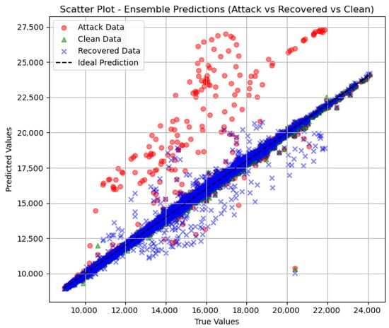
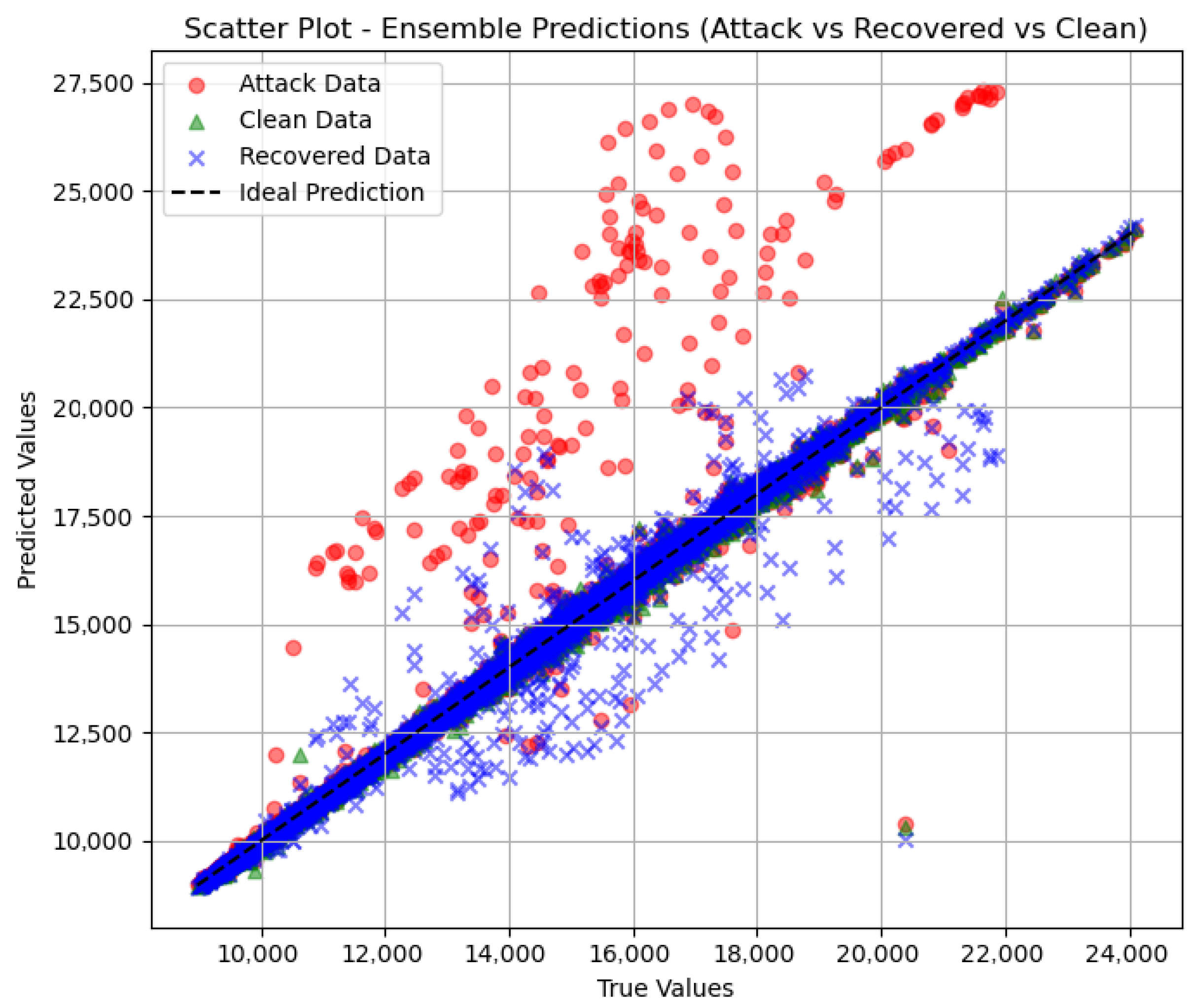
After data recovery, all models show significant improvement, with prediction accuracy approaching pre-attack levels. For example, the LSTM model’s $R^2$ increases from 0.9085 (compromised) to 0.9841 (recovered), and the MAE decreases from 184.24 to 122.07. As shown in Figure 11, the scatter plot simultaneously compares the predictions obtained from attacked data, recovered data, and original clean data against the ground-truth values. The predictions based on clean data are tightly clustered around the ideal prediction line ($y=x$), serving as a reference benchmark. Notably, the predictions obtained from the recovered data exhibit a high degree of overlap with those from the clean data and are also closely distributed along the diagonal. In contrast, predictions based on attacked data show significant dispersion and deviation from the ideal line. This visual comparison clearly demonstrates that the proposed recovery process effectively restores the data quality, enabling the forecasting model to recover prediction behavior that is highly consistent with the clean-data scenario.

Figure 11. Scatter Plot—Ensemble Predictions (Attack vs. Recovered).

Significantly, the proposed MO-WMA ensemble model consistently outperforms all individual models across all scenarios. In the recovered data scenario, it achieves the highest accuracy with $R^2=0.9851$ and MAE = 109.85, representing an $8.8\%$ reduction in MAE compared to the best-performing individual model. This indicates that the ensemble method can stabilize and further enhance forecasting performance even after data recovery.

Overall, the MO-WMA ensemble approach demonstrates superior performance across all three data scenarios. It significantly improves forecasting accuracy, robustness, and generalization capability relative to individual models. These results highlight the effectiveness of the proposed method in handling varying data quality conditions, making it well-suited for practical power load forecasting applications, particularly in environments where data integrity may be compromised.

5.3.4. Performance Analysis of MO-WMA and Baseline Ensembles

The proposed MO-WMA ensemble strategy employs a multi-objective evolutionary algorithm to optimize two key performance metrics: predictive accuracy ($R^2$) and error robustness (MAE). The optimization simultaneously maximizes $R^2$ (by minimizing $-R^2$) and minimizes MAE, aiming to identify weight configurations that perform well in both overall fit and local error control.

In contrast to traditional single-objective approaches, this dual-objective design provides a more comprehensive assessment of model performance, reducing the risk of overfitting or bias associated with optimizing a single criterion. The strategy explores the Pareto front of non-dominated solutions, and the optimal weight configuration is selected based on validation performance. This procedure enhances the robustness of the ensemble under varying data quality conditions.

As shown in Table 8, the MO-WMA ensemble outperforms all baseline ensemble methods. In the restored data scenario, it achieves the lowest MSE (107,478.93), RMSE (327.84), MAE (109.85), and MAPE (0.7359%), as well as the highest $R^2$ (0.9851). Compared to simple weighted averaging, MO-WMA reduces MSE by approximately 5.8% and improves $R^2$ by 0.09%, indicating a notable improvement in prediction accuracy.

Table 8. Performance Comparison of Different Ensemble Methods.

Method	MSE	RMSE	MAE	MAPE	${\mathit{R}}^2$
Simple Average	114,085.5759	337.7656	117.8953	0.0080	0.9842
MO-PSO	112,528.1597	335.4522	112.2550	0.0075	0.9844
MO-WOA	111,932.0610	334.5625	111.0449	0.0074	0.9845
WMA (Single Obj)	111,920.1778	334.5447	111.6006	0.0075	0.9845
MO-WMA (Proposed)	107,478.9265	327.8398	109.8532	0.0074	0.9851

Compared with other multi-objective optimization-based ensemble methods, such as MO-PSO [39] and MO-WOA [40], MO-WMA demonstrates clear advantages. For instance, it reduces MAE by 1.1% and increases $R^2$ by 0.06% relative to MO-WOA. Although the improvement in $R^2$ appears limited, MO-WMA achieves a notable reduction in MAE, indicating a consistent decrease in absolute prediction errors across the entire load sequence. Such error reductions enhance the reliability of short-term load forecasting and provide more accurate support for operational decision-making. These results indicate that MO-WMA more effectively captures load variation trends and minimizes local errors, thanks to its dual-objective design that simultaneously optimizes predictive accuracy ($R^2$) and error robustness (MAE), while identifying Pareto-optimal weight configurations for the ensemble.

Under challenging conditions, such as noisy or missing data, MO-WMA achieves lower forecasting errors and greater stability than baseline methods. These results confirm the robustness and adaptability of the approach, highlighting its potential for practical power system forecasting applications.

6. Conclusions

This paper addresses the challenges of false data injection (FDI) attacks in short-term load forecasting by proposing a collaborative detection and prediction framework based on temporal features and ensemble learning. Regarding the first research question, the framework employs a two-stage detection mechanism that effectively identifies and corrects compromised load data using only the intrinsic temporal and periodic characteristics of the load series, without relying on external covariates. Regarding the second research question, the ensemble forecasting strategy, optimized via a multi-objective algorithm, maintains and restores robust short-term load forecasting performance under attack scenarios, providing reliable inputs for power system dispatch. Future work will focus on enhancing the real-time performance and generalization capability of the framework, and extending it to multi-region, multivariate load forecasting scenarios with high penetration of renewable energy, thereby supporting the safe and stable operation of smart grids.

References

- Eren, Y.; Küçükdemiral, İ. A comprehensive review on deep learning approaches for short-term load forecasting. Renew. Sustain. Energy Rev. 2024, 189, 114031. [Google Scholar] [CrossRef] [Scilit]
- Cao, Z.; Wang, J.; Xia, Y. Combined electricity load-forecasting system based on weighted fuzzy time series and deep neural networks. Eng. Appl. Artif. Intell. 2024, 132, 108375. [Google Scholar] [CrossRef] [Scilit]
- Cui, Y.; Wu, T.; Zhang, Y. Load Frequency Control of Smart Grid Based on Data-Driven FDI Attacks Detection and Data Repair. IEEE Trans. Smart Grid 2025, 16, 5404–5415. [Google Scholar] [CrossRef] [Scilit]
- Rajkumar, V.S.; Ştefanov, A.; Torres, J.L.R.; Palensky, P. Dynamical analysis of power system cascading failures caused by cyber attacks. IEEE Trans. Ind. Inform. 2024, 20, 8807–8817. [Google Scholar] [CrossRef] [Scilit]
- Yue, M. An integrated anomaly detection method for load forecasting data under cyberattacks. In Proceedings of the 2017 IEEE Power & Energy Society General Meeting, Chicago, IL, USA, 16–20 July 2017; IEEE: Piscataway, NJ, USA, 2017; pp. 1–5. [Google Scholar] [CrossRef] [Scilit]
- Yue, M. Evaluation of a data analytic based anomaly detection method for load forecasting data. In Proceedings of the 2018 IEEE Power & Energy Society General Meeting (PESGM), Portland, OR, USA, 5–10 August 2018; IEEE: Piscataway, NJ, USA, 2018; pp. 1–5. [Google Scholar] [CrossRef] [Scilit]
- Oprea, S.V.; Bâra, A.; Puican, F.C.; Radu, I.C. Anomaly detection with machine learning algorithms and big data in electricity consumption. Sustainability 2021, 13, 10963. [Google Scholar] [CrossRef] [Scilit]
- Xu, L.; Wang, B.; Zhao, D.; Wu, X. DAN: Neural network based on dual attention for anomaly detection in ICS. Expert Syst. Appl. 2025, 263, 125766. [Google Scholar] [CrossRef] [Scilit]
- Duan, J.; Feng, J. Dynamic anomaly detection in blast furnace operations using a Transformer-Enhanced Isolation Forest framework. Eng. Appl. Artif. Intell. 2025, 159, 111724. [Google Scholar] [CrossRef] [Scilit]
- Wang, Z.; He, H.; Wan, Z.; Sun, Y. Coordinated topology attacks in smart grid using deep reinforcement learning. IEEE Trans. Ind. Inform. 2020, 17, 1407–1415. [Google Scholar] [CrossRef] [Scilit]
- Ayas, S.; Ayas, M.S.; Cavdar, B.; Sahin, A.K. Detecting cyberattacks based on deep neural network approaches in industrial control systems. J. Inf. Secur. Appl. 2025, 94, 104206. [Google Scholar] [CrossRef] [Scilit]
- Cui, M.; Wang, J.; Yue, M. Machine learning-based anomaly detection for load forecasting under cyberattacks. IEEE Trans. Smart Grid 2019, 10, 5724–5734. [Google Scholar] [CrossRef] [Scilit]
- Audibert, J.; Michiardi, P.; Guyard, F.; Marti, S.; Zuluaga, M.A. Usad: Unsupervised anomaly detection on multivariate time series. In Proceedings of the 26th ACM SIGKDD International Conference on Knowledge Discovery & Data Mining, Virtual, 23–27 August 2020; Association for Computing Machinery: New York, NY, USA, 2020; pp. 3395–3404. [Google Scholar] [CrossRef] [Scilit]
- Wang, X.; Yao, Z.; Papaefthymiou, M. A real-time electrical load forecasting and unsupervised anomaly detection framework. Appl. Energy 2023, 330, 120279. [Google Scholar] [CrossRef] [Scilit]
- Lei, T.; Gong, C.; Chen, G.; Ou, M.; Yang, K.; Li, J. A novel unsupervised framework for time series data anomaly detection via spectrum decomposition. Knowl.-Based Syst. 2023, 280, 111002. [Google Scholar] [CrossRef] [Scilit]
- Zhang, W.; Luo, C. Decomposition-based multi-scale transformer framework for time series anomaly detection. Neural Netw. 2025, 187, 107399. [Google Scholar] [CrossRef] [Scilit]
- Wang, X.; Zhu, H.; Luo, X.; Guan, X. Data-Driven-based Detection and Localization Framework against False Data Injection Attacks in DC Microgrids. IEEE Internet Things J. 2025, 12, 36079–36093. [Google Scholar] [CrossRef] [Scilit]
- Wang, Y.; Lu, Z.; Ma, J.; Jin, Q. Locational false data injection attack detection in smart grid using recursive variational graph auto-encoder. IEEE Internet Things J. 2025, 12, 13697–13708. [Google Scholar] [CrossRef] [Scilit]
- Yue, M.; Hong, T.; Wang, J. Descriptive analytics-based anomaly detection for cybersecure load forecasting. IEEE Trans. Smart Grid 2019, 10, 5964–5974. [Google Scholar] [CrossRef] [Scilit]
- Moradzadeh, A.; Mohammadpourfard, M.; Konstantinou, C.; Genc, I.; Kim, T.; Mohammadi-Ivatloo, B. Electric load forecasting under False Data Injection Attacks using deep learning. Energy Rep. 2022, 8, 9933–9945. [Google Scholar] [CrossRef] [Scilit]
- Luo, J.; Hong, T.; Fang, S.C. Benchmarking robustness of load forecasting models under data integrity attacks. Int. J. Forecast. 2018, 34, 89–104. [Google Scholar] [CrossRef] [Scilit]
- Luo, J.; Hong, T.; Fang, S.C. Robust regression models for load forecasting. IEEE Trans. Smart Grid 2018, 10, 5397–5404. [Google Scholar] [CrossRef] [Scilit]
- Jiao, J.; Tang, Z.; Zhang, P.; Yue, M.; Yan, J. Cyberattack-resilient load forecasting with adaptive robust regression. Int. J. Forecast. 2022, 38, 910–919. [Google Scholar] [CrossRef] [Scilit]
- Aflaki, A.; Gitizadeh, M.; Kantarci, B. Accuracy improvement of electrical load forecasting against new cyber-attack architectures. Sustain. Cities Soc. 2022, 77, 103523. [Google Scholar] [CrossRef] [Scilit]
- Luo, J.; Hong, T.; Gao, Z.; Fang, S.C. A robust support vector regression model for electric load forecasting. Int. J. Forecast. 2023, 39, 1005–1020. [Google Scholar] [CrossRef] [Scilit]
- Li, D.; Leung, M.F.; Tang, J.; Wang, Y.; Hu, J.; Wang, S. Generative self-supervised learning for cyberattack-resilient EV charging demand forecasting. IEEE Trans. Intell. Transp. Syst. 2025. early access. [Google Scholar] [CrossRef] [Scilit]
- He, Y.; Luo, J.; Zheng, Y. A novel ensemble support vector regression for load forecasting under data attacks. Energy 2025, 333, 137100. [Google Scholar] [CrossRef] [Scilit]
- Zheng, R.; Gu, J.; Jin, Z.; Peng, H.; Zhu, Y. Load forecasting under data corruption based on anomaly detection and combined robust regression. Int. Trans. Electr. Energy Syst. 2020, 30, e12103. [Google Scholar] [CrossRef] [Scilit]
- Ahmadi, A.; Nabipour, M.; Taheri, S.; Mohammadi-Ivatloo, B.; Vahidinasab, V. A new false data injection attack detection model for cyberattack resilient energy forecasting. IEEE Trans. Ind. Inform. 2022, 19, 371–381. [Google Scholar] [CrossRef] [Scilit]
- Zhao, X.; Ma, Z.; Shi, X.; Zou, S. Attack detection and mitigation scheme of load frequency control systems against false data injection attacks. IEEE Trans. Ind. Inform. 2024, 20, 9952–9962. [Google Scholar] [CrossRef] [Scilit]
- Chen, Z.; Du, C.; Zhang, B.; Yang, C.; Gui, W. A Cybersecure Distribution-Free Learning Model for Interval Forecasting of Power Load Under Cyberattacks. IEEE Trans. Ind. Inform. 2024, 21, 2540–2549. [Google Scholar] [CrossRef] [Scilit]
- Savchuk, S.; Doskich, S.; Gołda, P.; Rurak, A. The seasonal variations analysis of permanent GNSS station time series in the central-east of Europe. Remote Sens. 2023, 15, 3858. [Google Scholar] [CrossRef] [Scilit]
- Balasundaram, S.; Prasad, S.C. Robust twin support vector regression based on Huber loss function. Neural Comput. Appl. 2020, 32, 11285–11309. [Google Scholar] [CrossRef] [Scilit]
- He, F.; Zhou, J.; Feng, Z.K.; Liu, G.; Yang, Y. A hybrid short-term load forecasting model based on variational mode decomposition and long short-term memory networks considering relevant factors with Bayesian optimization algorithm. Appl. Energy 2019, 237, 103–116. [Google Scholar] [CrossRef] [Scilit]
- Huang, C.; Yang, M. Memory long and short term time series network for ultra-short-term photovoltaic power forecasting. Energy 2023, 279, 127961. [Google Scholar] [CrossRef] [Scilit]
- Ławryńczuk, M.; Zarzycki, K. LSTM and GRU type recurrent neural networks in model predictive control: A Review. Neurocomputing 2025, 632, 129712. [Google Scholar] [CrossRef] [Scilit]
- Ghasemi, M.; Deriche, M.; Trojovskỳ, P.; Mansor, Z.; Zare, M.; Trojovská, E.; Abualigah, L.; Ezugwu, A.E.; kadkhoda Mohammadi, S. An efficient bio-inspired algorithm based on humpback whale migration for constrained engineering optimization. Results Eng. 2025, 25, 104215. [Google Scholar] [CrossRef] [Scilit]
- Zong, B.; Song, Q.; Min, M.R.; Cheng, W.; Lumezanu, C.; Cho, D.; Chen, H. Deep autoencoding gaussian mixture model for unsupervised anomaly detection. In Proceedings of the International Conference on Learning Representations, Vancouver, BC, Canada, 30 April–3 May 2018. [Google Scholar]
- Karthika, S.; Rathika, P. An adaptive data compression technique based on optimal thresholding using multi-objective PSO algorithm for power system data. Appl. Soft Comput. 2024, 150, 111028. [Google Scholar] [CrossRef] [Scilit]
- Deng, L.; Liu, S. Deficiencies of the whale optimization algorithm and its validation method. Expert Syst. Appl. 2024, 237, 121544. [Google Scholar] [CrossRef] [Scilit]
Disclaimer/Publisher’s Note: The statements, opinions and data contained in all publications are solely those of the individual author(s) and contributor(s) and not of MDPI and/or the editor(s). MDPI and/or the editor(s) disclaim responsibility for any injury to people or property resulting from any ideas, methods, instructions or products referred to in the content. |
© 2026 by the authors. Licensee MDPI, Basel, Switzerland. This article is an open access article distributed under the terms and conditions of the Creative Commons Attribution (CC BY) license.