


Abstract
Randomness is crucial for our understanding of nature and indispensable in information processing tasks. In practical applications, assessing the quality of random numbers is crucial—particularly in cryptographic applications, where random numbers must exhibit statistical uniformity. Various statistical estimation methods have been developed to test the statistical characteristics of generated random numbers, enabling comprehensive evaluation of their statistical uniformity from multiple perspectives. Despite recent advances in quantum information providing physically well-characterized models for randomness quantification, distinction between different types of random numbers (including quantum random numbers) remains a challenging task, and statistical uniformity is rarely directly applicable to such discrimination scenarios. With the development of artificial intelligence technologies, the problem of random number discrimination is expected to draw on the paradigm of image classification in computer vision. This research proposes a machine learning-based randomness discrimination method, specifically addressing the challenge of quantum random number identification. Specifically, we design an image-based convolutional neural network (CNN) approach: one-dimensional random number sequences are converted into two-dimensional grayscale images, and binary classification of these images is achieved by capturing high-dimensional latent features that are undetectable via traditional statistical tests, thereby enabling effective random number discrimination. Experimental results demonstrate that, for the selected quantum random numbers, the proposed discrimination method successfully achieves two key distinctions: (1) between raw quantum random numbers and classical random numbers; and (2) between raw quantum random numbers and post-processed quantum random numbers—additionally revealing the role of statistical uniformity in these discrimination tasks. This achievement provides significant support for the design of randomness extraction protocols and the security assessment of quantum random number generators.
1. Introduction
Randomness is an indispensable resource in fundamental science and modern information processing. While classical randomness often relies on complex but deterministic processes, quantum mechanics provides a positive answer to the existence of intrinsic randomness [1,2]. Consequently, quantum random number generators (QRNGs), leveraging stochastic processes such as vacuum fluctuations [3,4,5,6,7,8,9,10,11] and Bell inequality violations [12,13,14], are regarded as the gold standard for generating information-theoretically private sequences [15,16].
In practice, a QRNG architecture typically consists of an entropy source that generates raw stochastic events, followed by a digitization process and a deterministic randomness extractor [17,18]. The extractor compresses raw digital bits into a shorter string of nearly perfect random bits [19]. However, ensuring the security and quality of this process remains a critical challenge; low-quality randomness can lead to catastrophic cryptographic failures [20,21,22,23].
Traditionally, the quality of generated randomness is evaluated using statistical test suites such as NIST [24], AIS 31 [25], and TestU01 [26]. While effective at verifying uniformity and decorrelation, these methods have three fundamental limitations. First, they treat the generator as a black box, ignoring the underlying physical process and requiring delicate, often unverifiable calibration of devices [9,27,28,29,30]. Second, well-designed pseudorandom number generators (PRNGs) can easily pass these tests despite having low entropy, as statistical suites often fail to capture subtle structural differences or long-range correlations [31]. Third, most tests are inapplicable to biased raw data, yet extractors can mask poor entropy sources by producing seemingly uniform outputs [15,17]. This creates an urgent need for evaluation methods that can distinguish the quantum origin of randomness without relying on physical models or post-processing.
Machine learning (ML) offers a promising paradigm to bridge this gap by automatically extracting high-dimensional latent features that are undetectable by traditional tests [31,32,33,34]. Recent works have utilized ML for entropy evaluation, cryptanalysis, and post-processing acceleration (see Table 1). Building on these advancements, we propose an image-based convolutional neural network (CNN) approach to QRNG distinction. By converting one-dimensional bitstreams into two-dimensional grayscale images, our model captures spatial patterns and structural features inherent to the generation mechanism. The primary contribution of this work is a robust distinction framework applied directly to raw data. We construct a comprehensive dataset including classical PRNGs, physical thermal noise, and multiple types of QRNGs (laser phase noise and device-independent Bell tests). Our results demonstrate that the proposed CNN method can effectively (1) partition random numbers into uniform and non-uniform groups; (2) distinguish between raw quantum data and classical noise; and (3) verify the quantum identity of a generator regardless of post-processing. This provides a powerful tool for the security assessment and verification of modern QRNG systems.
Table 1.
Representative works on quantum random number generators based on machine learning.
The remainder of this paper is organized as follows. Section 2 provides the preliminary knowledge regarding quantum random number generators (QRNGs) and convolutional neural networks (CNNs). Section 3 describes the proposed methodology, including the construction of the comprehensive dataset and the architecture of the improved LeNet-5 model. Section 4 presents and analyzes the experimental results, highlighting the discrimination performance and its correlation with traditional statistical tests. Finally, Section 5 concludes the paper and discusses potential directions for future research.
2. Preliminary
2.1. Random Number Generation
Classical random number generation (RNG) methodologies are broadly bifurcated into hardware-based physical sources and software-defined algorithmic schemes. Hardware-based implementations, such as those utilizing FPGA capacitive oscillators or SRAM voltage underscaling, leverage stochastic physical phenomena—including thermal noise and metastability—to achieve continuous generation and high entropy. While these hardware solutions offer robustness against digital switching noise, they remain sensitive to placement-and-routing constraints and are often susceptible to side-channel attacks (SCA). Conversely, software-based generators rely on deterministic algorithms like the Mersenne Twister or the PCG family, which provide exceptional statistical properties and high computational throughput. However, these algorithmic approaches are inherently insecure for cryptographic purposes due to their predictability and potential for state recovery. A comprehensive comparative analysis of these diverse platforms, highlighting their respective advantages and security risks, is presented in Table 2.
Table 2.
Comparative Analysis of Classical Random Number Generators (Software & Hardware).
2.2. Quantum Random Number Generator
Quantum random number generators generate true randomness by exploiting the intrinsic stochasticity of quantum mechanical processes, which is fundamentally different from classical pseudo-random number generators (PRNGs) that rely on deterministic algorithms with initial seeds. The core of QRNG lies in quantum entropy sources and subsequent measurement and digitization. The generation process typically includes the following components: First, a quantum entropy source inducing quantum stochastic processes (e.g., spontaneous emission in lasers, vacuum field fluctuations); Second, a quantum measurement converting quantum fluctuations into measurable physical quantities (e.g., optical intensity, voltage) via detectors; Third, a digitization procedure sampling the measured analog signals into digital data using analog-to-digital converters (ADCs); Finally, a randomness extractor processing raw digital data with deterministic algorithms (e.g., Toeplitz matrix hashing) to obtain uniformly distributed random bits. According to the trustworthiness of devices, QRNGs are mainly classified into three categories:
Trusted-device randomness generation: The trusted-device randomness generation process refers to the fact that the undergoing physical process is trusted and well-characterized. The quantum system to be measured and the quantum measurements are first calibrated, and the system losses and noise are also modeled. For this type of randomness generation process, the intrinsic randomness is evaluated simply by calculating the quantum coherence of the quantum system on the measurement basis. This evaluation varies in different protocols, and we shall provide detailed analyses later for the protocols we use in this work. However, if the system characterization is inaccurate or even false, the randomness evaluation shall fail.
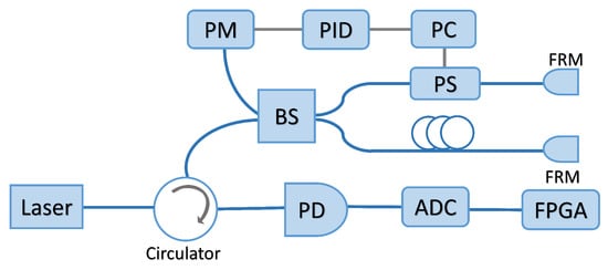
QRNGs based on laser phase noise (see Figure 1) have emerged as one of the leading approaches in the field, owing to their simple structures, clear operational principles and high generation rates, which utilize the phase fluctuations induced by spontaneous emission as a quantum entropy source to generate quantum random numbers. The photons emitted by a laser primarily originate from stimulated emission and spontaneous emission. Photons generated by stimulated emission are generally considered to have a fixed phase, while those produced by spontaneous emission exhibit a random phase. Consequently, the collective phase of photons generated by spontaneous emission fluctuates continuously over time, exhibiting intrinsic quantum randomness. Since direct measurement of phase fluctuations is inherently challenging, an interferometer is typically employed to convert phase fluctuations into measurable intensity fluctuations, which are then detected by a photodiode and subsequently converted into electrical signals. In this way, the quantum randomness inherent in spontaneous emission can be extracted and utilized to generate raw random numbers.
Figure 1.
Structure of the QRNG based on laser phase noise. BS: beam splitter, PS: phase shifter, FRM: Faraday rotator mirrors, PM: power meter, PID: proportional–integral–derivative, PC: piezoelectric controller, PD: photodiode, ADC: analog-to-digital converter, FPGA: field-programmable gate array.
The QRNG topology based on laser phase noise adopted in our work is mainly considered for the following two reasons: First, this topology has a simple structure, clear operational principles, and is easy for experimental implementation and data collection. It also features a high generation rate, making it one of the mainstream technical routes in the current QRNG field. Second, compared with other topologies (e.g., complex topologies based on vacuum fluctuations and Bell inequality violations), this topology has a clear classical noise interference mechanism, which is more conducive to verifying the ability of machine learning methods to distinguish between “quantum signals and classical noise.” Experimental results show that the quantum random numbers generated by this topology can effectively reflect the structural differences between quantum and classical random numbers, providing a typical and reliable data source for the discrimination task in our work.
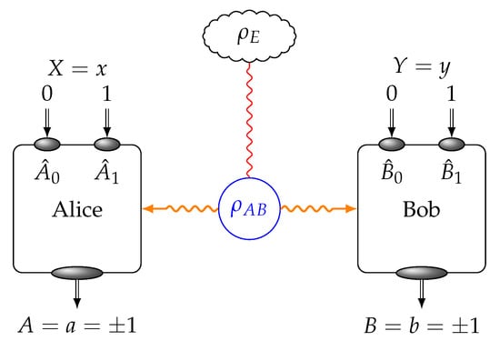
Device-independent (DI) randomness generation: In the quantum region, there exists specific correlation behaviour from which we can “self-test” the inner working status of the quantum devices without a prior characterisation. This phenomenon allows us to design (semi) device-independent quantum randomness generation protocols. In this work, we consider the device-independent quantum randomness generation based on the Bell tests. Intuitively, entanglement and non-commuting measurements are the necessary conditions for the violation of a Bell inequality. As entanglement can be interpreted as a special kind of multi-partite coherence, intrinsic randomness originates from breaking the entangled system. It is then possible to evaluate the amount of generated intrinsic randomness with respect to the Bell violation, as shown in Figure 2.
Figure 2.
Diagram of a Bell test setup.
In this work, we consider DI-QRNG based on the Clauser–Horne–Shimony–Holt (CHSH) Bell inequality [47]. As shown in Figure 2, two players, Alice and Bob, share a bipartite quantum state . Their state might be correlated with another party in the state . In the Bell test, Alice and Bob randomly choose the input settings , which correspond to the measurement of the observables . Their measurement devices generate outputs . Afterwards, Alice and Bob evaluate the following value,
In [48], a tight lower bound on the conditional min-entropy is analytically derived in terms of the Bell value,
However, if there is a loophole in the Bell test, this randomness evaluation result might fail. In a loophole-free Bell test, the following conditions are required:
- Non-Signaling: No information is communicated between Alice and Bob’s devices in a round.
- Free Will: The users have trusted local private randomness as the basis for their choices.
- Efficiency: The detection efficiency must be higher than a threshold to ensure the violation without assuming fair sampling.
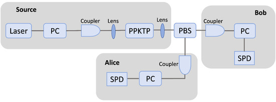
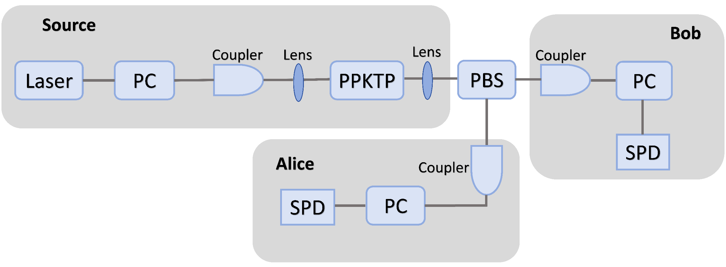
The optical experimental settings of DI-QRNG is shown in Figure 3.
Figure 3.
Experimental settings of DI-QRNG. SPD: single-photon detector, PC: polarization controller; PPKTP: periodically poled KTiOPO4; PBS: polarization beam splitter.
Semi-self-testing QRNG: Balances device trustworthiness and generation speed, serving as an intermediate category. This category typically includes source-independent QRNGs and measurement-device-independent QRNGs, which are not the focus of this work.
For post-processed QRNG (QRNG-Post-processed, DI-QRNG-Post-processed), we adopted the Toeplitz matrix hashing extractor. The extractor parameters are: matrix size = , hash function = SHA-256, and the output length is 50% of the input raw data length. This procedure effectively eliminates biases and correlations, resulting in uniformly distributed random bits that pass the NIST SP 800-22 test suite. These detailed descriptions and the new Figure 2 have been added to Section 2.1 (Quantum Random Number Generator) of the revised manuscript.
2.3. Convolutional Neural Network (CNN)
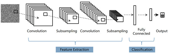
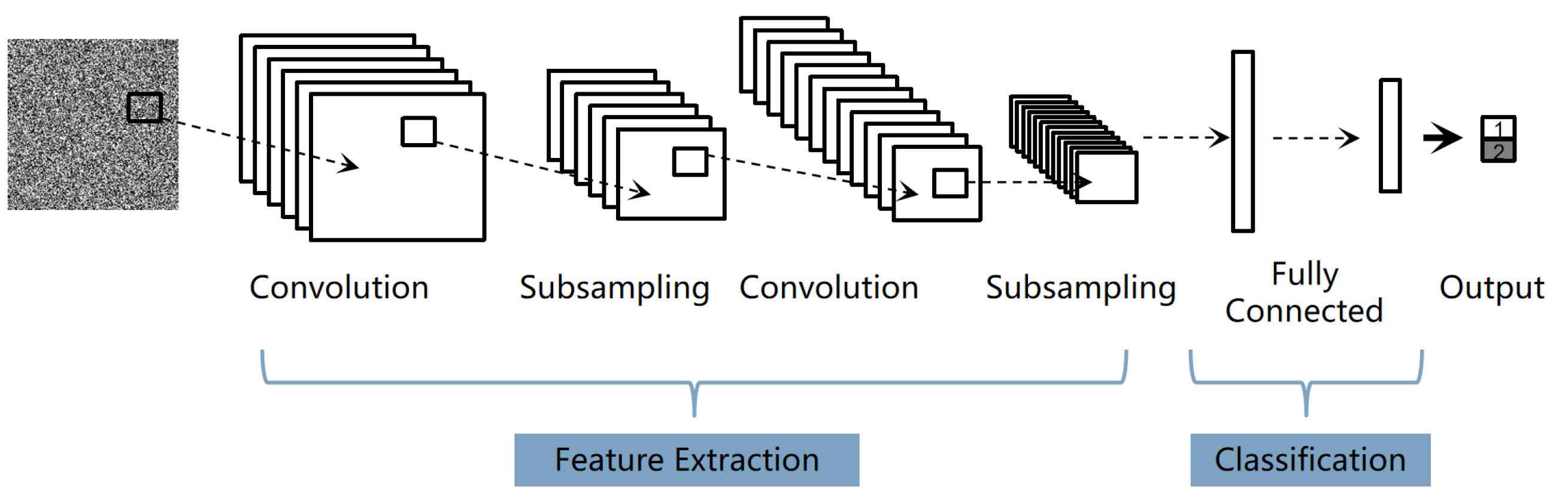
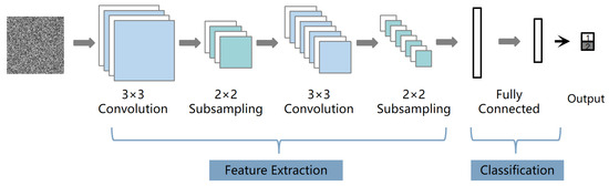
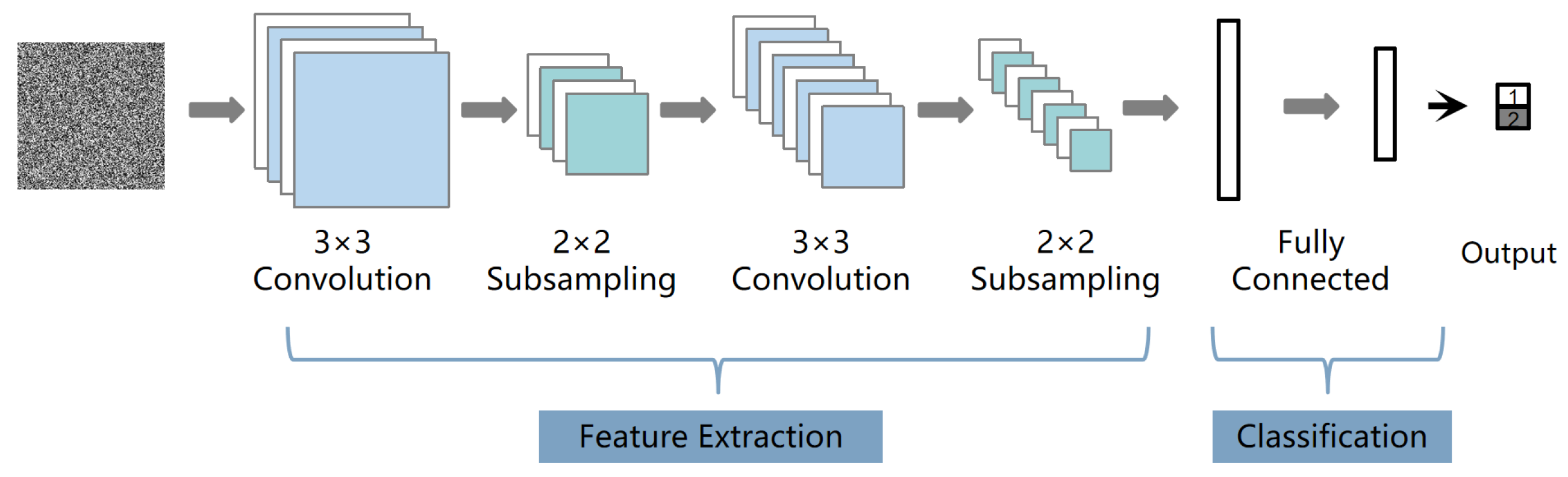
CNNs are deep learning models designed for grid-structured data (e.g., images), featuring local receptive fields, weight sharing, and pooling operations. A typical CNN consists of the following components (Figure 4): Convolutional layers: Extract hierarchical features from input data via convolution kernels. Each kernel slides over the input to compute feature maps, capturing local patterns (e.g., edges, textures in images). Activation functions: Introduce non-linearity to model complex relationships. The Rectified Linear Unit (ReLU) is widely used, defined as , which mitigates the vanishing gradient problem. Pooling layers: Reduce feature map dimensions while preserving key information. Max-pooling (taking the maximum value in a local window) is commonly adopted to enhance spatial invariance. Fully connected layers: Map high-dimensional features from convolutional/pooling layers to class labels for classification tasks.
Figure 4.
Structure of a typical CNN.
Compared with traditional statistical tests, CNNs offer unique advantages for random number distinction: Automatic feature extraction: No need for handcrafted features (e.g., frequency, linear complexity), automatically capturing high-dimensional latent patterns in random sequences. Strong representation ability: Deep network structures can model subtle structural differences between classical and quantum random numbers that are undetectable when using statistical methods. Adaptability to raw data: Directly process raw random data without relying on prior assumptions about distribution uniformity.
Random number sequences are one-dimensional (1D) binary streams, which are not suitable for CNN input. Converting 1D sequences into two-dimensional (2D) grayscale images leverages CNN’s powerful image recognition capabilities. Each bit in the sequence maps to a pixel (0 → black, 1 → white), and the 2D structure preserves the sequential correlation of the original data. This conversion enables CNN to capture spatial patterns corresponding to the intrinsic structure of random numbers, laying the foundation for effective distinction. We summarize representative machine learning techniques in Table 3.
Table 3.
Overview of machine learning technologies in the context of RNG analysis.
3. Methods
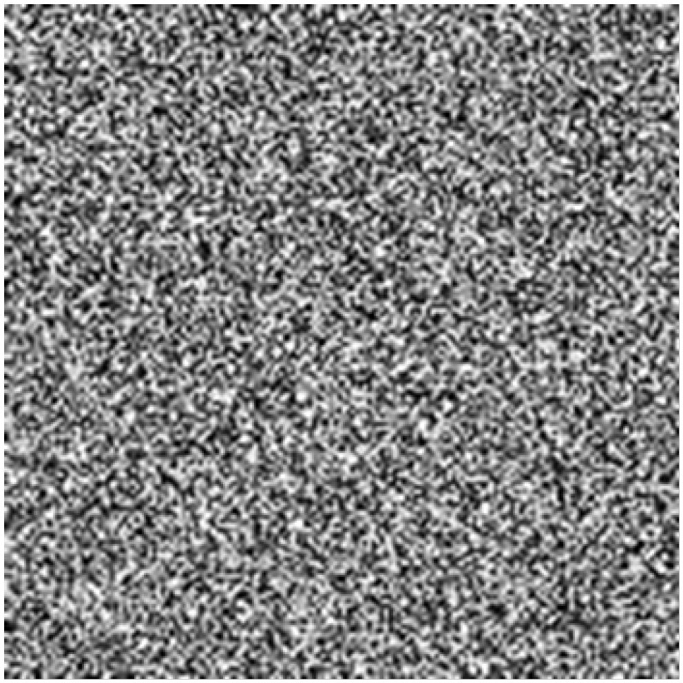
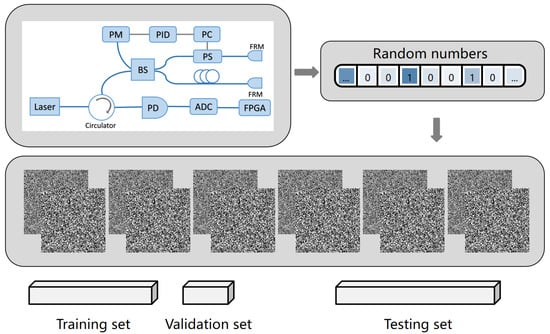
In this research, we address the core problems in QRNG distinction between classical and quantum random numbers. To this end, we collect a large number of datasets from thermal noise, physical random numbers, classical noise in the raw quantum random numbers generation stage, the raw quantum random numbers, and the final generated quantum random numbers—multiple types of classical/quantum random numbers for the distinction task. We leverage the image recognition capability of CNNs, converting one-dimensional random number sequences into two-dimensional images (Figure 5) to capture structural features that enable effective classification. The core idea of distinguishing classical and quantum random numbers is to convert one-dimensional random number sequences into two-dimensional images, leveraging the mature image recognition capabilities of machine learning models to achieve accurate binary and multi-class classification. Unlike traditional statistical test methods that rely on handcrafted features (e.g., frequency, serial correlation, linear complexity), this image-based approach automatically extracts high-dimensional latent features from random number sequences, thereby capturing subtle differences between classical and quantum randomness.
Figure 5.
Image representation of random numbers generated by LCG-PRNG.
3.1. Dataset
To ensure the generality and reliability of the discrimination model, a comprehensive dataset containing multiple types of random numbers was constructed, covering both classical pseudorandom numbers, classical physical random numbers, and quantum random numbers with different generation mechanisms. Specifically, the classical pseudorandom numbers included (1) Linear Congruential Generator pseudorandom numbers (LCG-PRNG), generated using the formula with standard parameters a = 1,103,515,245, c = 12,345, and ; (2) Mersenne Twister pseudorandom numbers (MT-PRNG), a widely used PRNG with a period of and excellent statistical properties; (3) Linux operating system pseudorandom numbers (LINUX-PRNG), sourced from the/dev/random interface, which aggregates environmental noise from hardware devices. The classical physical random numbers were physical thermal noise random numbers collected from a resistor thermal noise detection system at room temperature (298 K). The quantum random numbers included (1) trusted device quantum random numbers (1 GHz sampling rates), generated from the laser phase noise; (2) random numbers from classical noise in quantum random processes (1 GHz sampling rates), obtained by turning off the laser in the QRNG system; (3) device-independent quantum random numbers (DI-QRNG), generated based on Bell inequality violation without trusting the internal working of the quantum device.
Each type of random number was standardized to a size of 10 MB (equivalent to binary bits) to ensure sufficient data volume for model training and testing. The one-dimensional binary sequence was then converted into two-dimensional grayscale images using a reshape operation: each image was set to a resolution of 32 × 32 pixels (totaling 1024 pixels per image), where each pixel value corresponds to a single bit (0 or 1) in the random number sequence. The selection of an appropriate input image resolution is of paramount importance, and its rationale is grounded in the two core considerations detailed below. First, we prioritize data mapping consistency and sequence adaptability to ensure proper alignment between binary random number sequences and their corresponding spatial image representations. Each 32 × 32 image corresponds to a 1024-bit binary random number sequence, and this segmentation length is empirically validated as reasonable: it preserves the intrinsic local sequential correlations inherent to the random number sequences while avoiding excessive computational overhead. Second, the 32 × 32 image resolution achieves the optimal tradeoff between model discrimination performance and computational efficiency for our specific task. Preliminary comparative experiments were conducted using alternative image resolutions (16 × 16 and 64 × 64) for benchmarking. The 16 × 16 resolution induces the loss of critical fine-grained features, leading to a notable decline in discrimination accuracy. Conversely, scaling to 64 × 64 resolution doubles the computational burden while creating a negligible gain in discrimination accuracy. Accordingly, the 32 × 32 resolution is formally validated as the optimal choice, striking a well-rounded balance among feature preservation, discriminative capability, and computational efficiency.
We have explicitly elaborated on the sequential reshaping operation that transforms one-dimensional (1D) random number sequences into two-dimensional (2D) images following a fixed ordering rule: the first 32 bits form the first row of the 2D image, the ensuing 32 bits sequentially constitute the second row, and this patterned arrangement is iteratively executed in a consistent manner. This transformation preserves the inherent temporal correlations of the original 1D sequences within the spatial structure of the generated 2D images. Furthermore, we observe that scrambling the bit order prior to the reshaping procedure induces complete disorder in model inference and renders the model entirely non-functional. These experimental results demonstrate that the spatial correlations embedded in the 2D images are a direct manifestation of the temporal correlations inherent in the original random number sequences.
To ensure experimental reproducibility, a fixed random seed of 42 was used for all dataset splitting steps (implemented via numpy.random.seed(42) and sklearn.model_ selection.train_ test_ split(random_ state = 42) in Python 3.12. Each random number type contains 81,920 32 × 32 image samples, calculated as 10 MB/1024 bytes = 81,920, which were randomly split into a training set and a test set at a 1:1 ratio (40,960 samples per class for training and 40,960 for testing) to avoid overfitting and ensure the model’s generalization ability to unseen data; in addition, a validation set of 4096 samples per class was randomly extracted from of the training set with no sample overlap, allowing the model’s performance to be monitored during training and hyperparameters to be adjusted in a timely manner.
The complete data pipeline was constructed as follows: raw random bitstreams (10 megabytes per class) were first reshaped into 32 × 32 two-dimensional grayscale images (where 0 represents a black pixel, and 1 represents a white pixel) in accordance with the row-major order rule; subsequently, the image dataset was normalized to scale the pixel values to the range of ; next, the dataset was split into training, test, and validation subsets with a fixed random seed of 42 to ensure reproducibility; finally, the split datasets were converted into the tf.data.Dataset format compatible with TensorFlow, and the efficiency of data loading was optimized by applying prefetch (buffer_size = tf.data.AUTOTUNE) and shuffle (buffer_size = 10,000) operations, with no data augmentation performed, given that the structural features of random number images cannot be disturbed.
3.2. Training Process
As a foundational model of convolutional neural networks (CNNs), traditional LeNet-5 has achieved groundbreaking breakthroughs in early tasks such as handwritten digit recognition, relying on its concise hierarchical architecture of convolution–pooling–full connection. However, its inherent limitations lead to insufficient feature representation capability and generalization performance of the model, making it difficult to be directly adapted to complex classification tasks with specific data distribution characteristics, such as random number discrimination. To address this issue, this study adopts the improved LeNet-5 model, and specifically through the integration of multi-scale convolutional features, unsaturated substitution of activation functions, and targeted implementation of regularization strategies, the model’s classification accuracy and robustness in random number discrimination tasks are significantly enhanced.
For the binary classification task utilizing the improved LeNet-5, the input consists of 32 × 32 RGB images with a batch size of 64, corresponding to an initial input tensor shape of [64, 32, 32, 3] in Figure 6 (where the dimensions represent [batch size, height, width, channels], and the 3 channels are derived from the RGB image properties). This input tensor remains unchanged after passing through the input layer, which solely performs data normalization without involving any trainable parameters. Subsequently, the first convolutional layer—equipped with 32 3 × 3 kernels, a padding of 1, and a stride of 1—processes the input tensor, yielding an output tensor of [64, 32, 32, 32]. Here, the channel count increases from 3 to 32, which equals the number of convolutional kernels. The ReLU activation function applied immediately afterward introduces non-linearity without altering the tensor shape. The following max pooling layer 1, configured with a 2 × 2 kernel, a stride of 2, and no padding, downsamples the feature maps, reducing the spatial dimensions from 32 × 32 to 16 × 16 while preserving the channel count at 32, thus outputting a tensor of [64, 16, 16, 32]. Next, the second convolutional layer (featuring 64 3 × 3 kernels, a padding of 1, and a stride of 1) further extracts high-level spatial features. After ReLU activation, the tensor shape transforms to [64, 16, 16, 64], with the channel count increasing from 32 to 64. The subsequent max pooling layer 2, identical in configuration to the first pooling layer (2 × 2 kernel, stride = 2, no padding), downsamples the spatial dimensions again to 8 × 8, resulting in an output tensor of [64, 8, 8, 64], with the channel count remaining 64. The flatten layer then converts the four-dimensional feature maps into a 2-dimensional vector; the length of this vector is calculated as 8 × 8 × 64 = 4096, leading to an output tensor of [64, 4096]. This two-dimensional vector is fed into the first fully connected layer (FC1), which has an input dimension of 4096 and an output dimension of 512. After ReLU activation, FC1 produces an output tensor of [64, 512], serving to integrate the global feature information extracted from the convolutional and pooling layers. The second fully connected layer (FC2), acting as the output layer, has an input dimension of 512 and an output dimension of 2 (matching the number of classes in the binary classification task), ultimately generating an output tensor of [64, 2]. Finally, this tensor is processed by the Softmax layer to convert it into a probability distribution (where the sum of probabilities for the two classes is 1), while maintaining the tensor shape of [64, 2]. The output values of this tensor represent the predicted probabilities that the input sample belongs to each of the two classes. We illustrate the whole process in Figure 7.
Figure 6.
Data preparation and processing (using QRNG based on laser phase noise as an example).
Figure 7.
Processing flow for binary classification of random numbers based on an improved LeNet-5 CNN.
For the basic binary classification task with balanced sample distribution (e.g., classifying random numbers into two distinct classes), the improved LeNet-5 model employs the Binary Cross-Entropy (BCE) Loss as the core objective function for training. This loss function is a standard choice for balanced binary classification scenarios, as it effectively quantifies the discrepancy between the model’s predicted probability distribution and the ground-truth label distribution, without introducing additional weight adjustments for sample imbalance. To align with the binary classification task, the output layer of the original LeNet-5 (designed for multi-class classification with a multi-neuron Softmax layer) is improved in the improved version: the output layer is simplified to a single neuron with a Sigmoid activation function, which maps the raw logits (unnormalized scores) of the model to the range [0, 1]. This mapping directly yields the predicted probability that a given sample belongs to Class A (positive class), which is required for the computation of BCE Loss. The mathematical formulation of the BCE Loss is given in Equation (3):
where N denotes the batch size (number of training samples in a single mini-batch), and represents the ground-truth label of the i-th sample, with indicating one class and indicating another class. is the predicted probability that the i-th sample belongs to the one class, where is the raw output (logit) of the improved LeNet-5’s output layer, and denotes the Sigmoid activation function. During the training process, the parameters of the improved LeNet-5 are updated via backpropagation to minimize , thereby optimizing the model’s ability in the balanced binary classification task of random number discrimination.
4. Results
4.1. Model Selection and Parameter Settings
The experimental hardware environment consists of an NVIDIA RTX 3090 (24 GB VRAM) GPU, an Intel Core i9-12900K (3.2 GHz, 16 cores) CPU, 64 GB of DDR5 RAM, and the Ubuntu 20.04 LTS operating system, with TensorFlow 2.2.0, CUDA 11.0, and cuDNN 8.0 adopted as the deep learning framework and corresponding acceleration libraries. All experiments adopt a fixed batch size of 64, and the per-epoch and total wall-clock training times are measured under the above hardware configuration; the improved LeNet-5 takes approximately 2 h to train on a single NVIDIA RTX 3090 GPU, with a per-epoch training time of about 2.5 min. In this study, we employ a improved LeNet-5 architecture that presents obvious performance advantages over the vanilla LeNet-5 model, which has prominent limitations when applied to random number image classification. Specifically, the original network only deploys single-scale 5 × 5 convolutional kernels and fails to simultaneously extract the fine-grained local characteristics and global structural patterns inherent to random number images; adopts the Sigmoid saturated activation function that gives rise to the vanishing gradient problem in deep network training, thus hindering model convergence and resulting in unsatisfactory classification accuracy; and lacks any built-in regularization mechanisms, making it highly prone to overfitting when trained on large-scale random number image datasets.
To address the aforementioned limitations, we introduce two targeted optimization strategies in the improved network: we parallelly integrate 3 × 3 and 2 × 2 multi-scale convolutional kernels to capture multi-level features of random number images, which effectively remedies the defect that single-scale convolutional kernels fail to extract comprehensive visual features; furthermore, we embed L2 regularization with a weight decay coefficient of 0.0005 and dropout layers with a dropout rate of 0.2 into the fully connected layers, which suppresses model overfitting and improves the generalization performance of the network on test datasets.
The rationale for adopting our improved LeNet-5 model over more advanced architectures such as ResNet-18 is threefold. Primarily, LeNet-5 was originally developed for small-scale image classification tasks typified by 32 × 32 MNIST handwritten digit images, making it perfectly compatible with the resolution of the binary random number images in this study; conversely, modern networks like ResNet are engineered for large 224 × 224 images (e.g., ImageNet datasets) and demand a massive number of parameters for feature extraction, which is redundant for the structurally simple random number images. Additionally, preliminary experiments demonstrate that ResNet-18 yields a classification accuracy of 96.5% on our dataset, nearly on par with the 96.2% achieved by our improved LeNet-5, yet ResNet-18 contains 11 million parameters—roughly 50 times the 220,000 parameters of our improved model—and such excessive parametric capacity substantially raises the overfitting risk on simple datasets. Finally, the improved LeNet-5 finishes training in just 2 h on a single NVIDIA RTX 3090 GPU, while ResNet-18 takes 10 h under identical hardware conditions, and this distinct computational efficiency advantage better facilitates the practical application of the proposed discrimination method in the security evaluation of quantum random number generators (see Table 4).
Table 4.
Architecture Details and Parameter Counts of Original and Improved LeNet-5.
All model hyperparameters in this study were determined via grid search, and model performance was evaluated on the validation set using 5-fold cross-validation to select the parameter combination with the highest validation accuracy and optimal generalization ability. The key hyperparameters of the model were systematically optimized, and their search ranges, number of trials, final values, and selection criteria are summarized as follows: for the learning rate, four candidate values (0.01, 0.001, 0.0001, 0.00001) were tested in 4 independent trials, and 0.0001 was determined as the optimal value because 0.01 and 0.001 led to excessively fast convergence and severe overfitting, 0.00001 resulted in overly slow convergence, and 0.0001 achieved a favorable balance between convergence speed and classification accuracy; for the L2 regularization coefficient, three values (0.0001, 0.0005, 0.001) were evaluated in 3 trials, with 0.0005 selected as the final value since 0.0001 provided insufficient regularization, 0.001 caused underfitting due to excessive regularization, and 0.0005 effectively suppressed overfitting without sacrificing model accuracy; for the Dropout rate, three candidate values (0.1, 0.2, 0.3) were examined in 3 trials, and 0.2 was chosen as the optimal value as 0.1 exhibited a weak effect on overfitting suppression, 0.3 led to excessive feature loss, and 0.2 achieved the best trade-off between feature preservation and overfitting reduction; for the training epochs, three values (30, 40, 50) were tested in 3 trials, and 50 epochs were finally adopted, which can ensure sufficient convergence of the model when combined with the early stopping strategy (training terminates if no performance improvement occurs within 5 consecutive epochs). Additionally, the Adam optimizer with default hyperparameters () is adopted for network parameter optimization, and Binary Cross-Entropy (BCE) Loss is employed as the loss function for the binary classification task in this work.
To verify whether the performance differences between each model and the improved LeNet-5 are statistically significant, 10 independent repeated experiments were conducted for all models (with the random seed fixed and only the random partition of the dataset altered). A paired t-test was employed to analyze the accuracy differences between the improved LeNet-5 and other models, with the significance level set to (where p < 0.05 indicates a significant difference, and p < 0.01 indicates an extremely significant difference). The test results are presented in the following Table 5.
Table 5.
Statistical significance test results of model comparison (Improved LeNet-5 as the benchmark).
The results reveal that the performance discrepancies between the improved LeNet 5 and the original LeNet 5, MLP, and SVM all reach a statistically highly significant level, which validates that the proposed architectural modification strategies can effectively enhance the discriminative capability of the model. By contrast, no statistically significant accuracy difference is observed between the improved LeNet 5 and ResNet 18. Considering that ResNet 18 has substantially more parameters (11 million) than the improved LeNet 5 (220,000) and requires more than five times the training time, it is conclusively demonstrated that the improved LeNet 5 serves as a more advantageous lightweight model.
Meanwhile, we elaborate on the results of statistical randomness tests in this section. Statistical test suites such as the NIST SP 800-22 test can determine the randomness of a target sequence solely based on its statistical indicators, yet such judgments are intrinsically qualitative, which only enables a rough classification of samples into statistically uniform distribution groups and statistically non-uniform distribution groups for discrimination tasks. In contrast, our convolutional neural network (CNN)-based discrimination approach not only validates the qualitative classification results of the statistically uniform and non-uniform groups, but also provides quantitative discrimination accuracy on this basis.
Finally, we implement targeted strategies to further alleviate the influence of overfitting risks on experimental validity, a key issue that often compromises the generalization capacity of deep learning models. Experimental results demonstrate that our improved LeNet-5 model achieves a classification accuracy of 96.2% on the training set and 95.8% on the independent validation set, with a marginal accuracy gap of only 0.4% between the two datasets. This negligible performance difference conclusively verifies that the model does not suffer from overfitting and retains superior generalization ability throughout training. Such favorable anti-overfitting behavior stems from the synergistic effect of the combined optimization strategies adopted in this work, namely, L2 regularization, dropout layers embedded in the fully connected modules, and the early stopping mechanism.
4.2. Binary Discrimination Results and Analysis
Table 6 summarizes the pairwise discrimination results of the 7 random number types (type correspondence: 1 = LCG-PRNG, 2 = MT-PRNG, 3 = LINUX-PRNG, 4 = Thermal Noise, 5 = QRNG-RAW, 6 = QRNG-Classical Noise-RAW, 7 = DI-QRNG-RAW.), where “Y” denotes effective discrimination (test set discrimination rate > 95 %), “N” denotes indistinguishability (discrimination rate ∼50%, consistent with random guessing), and blank cells correspond to self-comparison (excluded from analysis).
Table 6.
Pairwise discrimination results and NIST test results of 7 types of random number types. “Y” = effective discrimination; “N” = indistinguishability; “P” = pass; “F” = fail; blank = self-comparison. Type correspondence: 1 = LCG-PRNG, 2 = MT-PRNG, 3 = LINUX-PRNG, 4 = Thermal Noise, 5 = QRNG-Raw, 6 = QRNG-Classical Noise-Raw, 7 = DI-QRNG-Raw.
As seen in the table, a distinct bipartition emerges in the discrinination performance: the first four types (LCG-PRNG, MT-PRNG, LINUX-PRNG, and Thermal Noise) are mutually indistinguishable (marked “N”), which aligns with their uniformly distributed statistical properties—their converted 2D images lack unique structural features, so the CNN cannot capture differentiable latent patterns (as confirmed by LCG-PRNG passing all national cryptographic statistical tests). In contrast, these four uniform-distribution random numbers can all be effectively distinguished (marked “Y”) from the remaining three types (QRNG-Raw, QRNG-Classical Noise-Raw, DI-QRNG-Raw), whose non-uniform statistical distributions (e.g., the skewed distribution of QRNG-Classical Noise-Raw) introduce distinct spatial features into their 2D image representations. Notably, QRNG-RAW, QRNG-Classical Noise-RAW, and DI-QRNG-RAW not only distinguish from the uniform-distribution group but also from each other—this confirms that their non-uniformities carry unique, CNN-capturable feature information. Overall, these results verify that our image-based CNN approach effectively identifies subtle differences between random numbers with distinct statistical properties, particularly separating non-uniformly distributed (raw quantum random numbers) from uniformly distributed ones. We also perform NIST tests for all the 7 types of random numbers according to NIST SP 800-22. The distinction results align well with the NIST test result, i.e., the last three types of random numbers fail to pass the NIST test, while the first four types succeed. We also make a distinction between the QRNGs before and after post-processing (see Table 7), which are relabeled as (1 = QRNG-Post-processed, 2 = QRNG-Classical Noise-Post-processed, 3 = DI-QRNG-Post-processed, 4 = QRNG-Raw, 5 = QRNG-Classical Noise-Raw, 6 = DI-QRNG-Raw). It turns out that after processing, all three types of QRNGs become indistinguishable and can pass the NIST test.
Table 7.
Pairwise discrimination results and NIST test results of QRNGs before and after post-processing. “Y” = effective discrimination; “N” = indistinguishability; “P” = pass; “F” = fail; blank = self-comparison. Type of correspondence: 1 = QRNG–Post-processed, 2 = QRNG–Classical Noise–Post-processed, 3 = DI-QRNG–Post-processed, 4 = QRNG–Raw, 5 = QRNG–Classical Noise–Raw, 6 = DI-QRNG–Raw.
Thus far, we have tentatively confirmed the important role of statistical uniformity in random number discrimination tasks: i.e., for the binary discrimination task involving classical and quantum random numbers, if at least one of the two types fails to pass the NIST statistical tests, the convolutional neural network (CNN) model proposed in this research is conducive to achieving the discrimination task, with a critical prerequisite that the generation principles of the two types of random numbers exhibit significant differences; conversely, if the two types of random numbers share the same generation principle and only have minor differences in certain generation parameters (e.g., sampling rates of 500 M samples/s and 600 M samples/s), they remain difficult to distinguish, even though neither passes the NIST statistical tests. Additionally, the method proposed in this research is applicable to the quantum random numbers with different generation principles selected herein, while its applicability to those with other principles requires further testing. To further verify the contribution of statistical uniformity to random number discrimination, we have restricted the discrimination task exclusively to different types of quantum random numbers—for instance, selecting raw quantum random numbers and their corresponding post-processed counterparts for discrimination.
Conducting comparative experiments between biased, unprocessed classical random numbers and uniformly distributed counterparts holds substantial reference significance. Given that thermal noise random number data necessitates post-processing to eliminate inherent biases, we further performed such a comparative experiment, and the results corroborated the effectiveness of our proposed technique. Specifically, we utilized thermal noise random numbers subjected to basic denoising as the foundation, and introduced controllable biases by adjusting the sampling threshold of the Analog-to-Digital Converter (ADC) to construct biased unprocessed classical random numbers—for instance, tuning the proportion of 0-bits to 70% and that of 1-bits to 30%. Subsequently, we employed a pre-trained convolutional neural network (CNN) model to perform classification tasks on the biased unprocessed thermal noise random numbers versus three types of uniformly distributed classical random numbers, namely, thermal noise random numbers, Linear Congruential Generator pseudo-random numbers (LCG-PRNG), and Mersenne Twister pseudo-random numbers (MT-PRNG). Experimental results demonstrated that the model achieved an average classification accuracy of 96.7% for the two categories of random numbers (see Table 8). This finding indicates that our proposed technique is not only sensitive to the quantum or classical origin of randomness but also capable of effectively distinguishing between biased and uniformly distributed random numbers within the classical random number domain.
Table 8.
Comparative experiments between biased unprocessed classical random numbers and uniformly distributed counterparts. “Y” = effective discrimination; “N” = indistinguishability; “P” = pass; “F” = fail; blank = self-comparison. Type of correspondence: 1 = LCG–PRNG, 2 = MT–PRNG, 3 = thermal noise, 4 = thermal noise (biased).
A critical consideration in this research is whether the classifier can distinguish post-processed QRNG from classical PRNGs, as both exhibit high statistical uniformity. We believe our work has significant potential in this area. The core advantage of the CNN-based approach lies in its ability to capture generation-mechanism-dependent structural features rather than merely distinguishing biased vs. uniform distributions [31,32]. Classical random numbers (e.g., LCG-PRNG, MT-PRNG) are generated by deterministic algorithms with inherent periodicity or hidden correlations—even if they pass statistical uniformity tests such as NIST SP 800-22, their high-dimensional latent patterns (e.g., long-range sequential correlations) differ fundamentally from post-processed QRNG [26,31]. Post-processed QRNG is essentially unpredictable and aperiodic due to the fundamental laws of quantum mechanics [15,19]. By mapping these bitstreams into 2D spatial features, the CNN can potentially exploit these big structural differences that are invisible to 1D statistical estimators, providing a path for verifying “true” randomness even after extraction.
5. Conclusions
We propose an image-based convolutional neural network (CNN) method for distinguishing quantum random numbers (QRNGs) from classical random numbers. By converting one-dimensional random number sequences into two-dimensional grayscale images, the CNN effectively captures high-dimensional latent features that elude traditional statistical tests, successfully achieving two key distinctions: (1) between raw quantum random numbers and classical random numbers and (2) between raw quantum random numbers and post-processed quantum random numbers.
Our distinction method successfully partitions random numbers into uniform and non-uniform statistical distribution groups. Uniformly distributed random numbers—including classical pseudorandom numbers (LCG–PRNG, MT-PRNG, LINUX–PRNG), classical physical thermal noise, and trusted-post-processed-device QRNGs—are mutually indistinguishable. In contrast, non-uniformly distributed random numbers (raw quantum random numbers) can be reliably distinguished from the uniform group and even from each other. This demonstrates the method’s ability to reveal structural differences related to generation mechanisms, providing a new tool for verifying the quantum origin of random numbers.
The proposed approach avoids the limitations of physical model assumptions (which are often unprovable). It directly processes raw data, making it applicable to randomness extraction protocols and QRNG security assessment. However, uniformly distributed quantum random numbers cannot yet be distinguished from high-quality classical random numbers—a limitation that future work may address with more advanced feature extraction methods (e.g., deeper CNN architectures and transformer-based models).
Author Contributions
Conceptualization, Y.H.; Methodology, Y.H.; Validation, Y.H.; Formal analysis, Y.H. and T.P.; Resources, F.Z.; Data curation, T.P. and F.Z.; Writing – original draft, F.Z.; Writing – review & editing, Y.H.; Visualization, T.P.; Project administration, Y.H. All authors have read and agreed to the published version of the manuscript.
Funding
This research received no external funding.
Data Availability Statement
All experimental code and the complete raw dataset of this study, together with the data underlying the plots and other findings presented in this paper, are available from the corresponding author upon reasonable request.
Acknowledgments
We thank Yangyang Fei for the helpful discussion.
Conflicts of Interest
The authors declare no conflicts of interest.
References
- Bauke, H.; Mertens, S. Random numbers for large-scale distributed Monte Carlo simulations. Phys. Rev. E 2007, 75, 066701. [Google Scholar] [CrossRef] [Scilit]
- Stipcevic, M. Quantum random number generators and their applications in cryptography. In Proceedings of the Advanced Photon Counting Techniques VI; Itzler, M.A., Ed.; International Society for Optics and Photonics, SPIE: Washington, DC, USA, 2012; Volume 8375, p. 837504. [Google Scholar]
- Zhou, H.; Yuan, X.; Ma, X. Randomness generation based on spontaneous emissions of lasers. Phys. Rev. A 2015, 91, 062316. [Google Scholar] [CrossRef] [Scilit]
- Nie, Y.Q.; Huang, L.; Liu, Y.; Payne, F.; Zhang, J.; Pan, J.W. The generation of 68 Gbps quantum random number by measuring laser phase fluctuations. Rev. Sci. Instrum. 2015, 86, 063105. [Google Scholar] [CrossRef] [Scilit]
- Shen, Y.; Tian, L.; Zou, H. Practical quantum random number generator based on measuring the shot noise of vacuum states. Phys. Rev. A 2010, 81, 063814. [Google Scholar] [CrossRef] [Scilit]
- Qi, B.; Chi, Y.M.; Lo, H.K.; Qian, L. High-speed quantum random number generation by measuring phase noise of a single-mode laser. Opt. Lett. 2010, 35, 312–314. [Google Scholar] [CrossRef] [Scilit]
- Guo, H.; Tang, W.; Liu, Y.; Wei, W. Truly random number generation based on measurement of phase noise of a laser. Phys. Rev. E 2010, 81, 051137. [Google Scholar] [CrossRef] [Scilit]
- Gabriel, C.; Wittmann, C.; Sych, D.; Dong, R.; Mauerer, W.; Andersen, U.L.; Marquardt, C.; Leuchs, G. A generator for unique quantum random numbers based on vacuum states. Nat. Photonics 2010, 4, 711–715. [Google Scholar] [CrossRef] [Scilit]
- Huang, W.; Zhang, Y.; Zheng, Z.; Li, Y.; Xu, B.; Yu, S. Practical security analysis of a continuous-variable quantum random-number generator with a noisy local oscillator. Phys. Rev. A 2020, 102, 012422. [Google Scholar] [CrossRef] [Scilit]
- Bruynsteen, C.; Gehring, T.; Lupo, C.; Bauwelinck, J.; Yin, X. 100-Gbit/s Integrated Quantum Random Number Generator Based on Vacuum Fluctuations. PRX Quantum 2023, 4, 010330. [Google Scholar] [CrossRef] [Scilit]
- Li, Y.H.; Fei, Y.Y.; Wang, W.L.; Meng, X.D.; Wang, H.; Duan, Q.H.; Han, Y.; Ma, Z. Effect of external magnetic fields on practical quantum random number generator. EPJ Quantum Technol. 2023, 10, 49. [Google Scholar] [CrossRef] [Scilit]
- Pironio, S.; Acín, A.; Massar, S.; de La Giroday, A.B.; Matsukevich, D.N.; Maunz, P.; Olmschenk, S.; Hayes, D.; Luo, L.; Manning, T.A.; et al. Random numbers certified by Bell’s theorem. Nature 2010, 464, 1021–1024. [Google Scholar] [CrossRef] [Scilit]
- Liu, Y.; Yuan, X.; Li, M.H.; Zhang, W.; Zhao, Q.; Zhong, J.; Cao, Y.; Li, Y.H.; Chen, L.K.; Li, H.; et al. High-Speed Device-Independent Quantum Random Number Generation without a Detection Loophole. Phys. Rev. Lett. 2018, 120, 010503. [Google Scholar] [CrossRef] [Scilit]
- Liu, W.Z.; Li, M.H.; Ragy, S.; Zhao, S.R.; Bai, B.; Liu, Y.; Brown, P.J.; Zhang, J.; Colbeck, R.; Fan, J.; et al. Device-independent randomness expansion against quantum side information. Nat. Phys. 2021, 17, 448–451. [Google Scholar] [CrossRef] [Scilit]
- Ma, X.; Yuan, X.; Cao, Z.; Qi, B.; Zhang, Z. Quantum random number generation. npj Quantum Inf. 2016, 2, 1–9. [Google Scholar] [CrossRef] [Scilit]
- Herrero-Collantes, M.; Garcia-Escartin, J.C. Quantum random number generators. Rev. Mod. Phys. 2017, 89, 015004. [Google Scholar] [CrossRef] [Scilit]
- Ma, X.; Xu, F.; Xu, H.; Tan, X.; Qi, B.; Lo, H.K. Postprocessing for quantum random-number generators: Entropy evaluation and randomness extraction. Phys. Rev. A 2013, 87, 062327. [Google Scholar] [CrossRef] [Scilit]
- De, A.; Portmann, C.; Vidick, T.; Renner, R. Trevisan’s extractor in the presence of quantum side information. SIAM J. Comput. 2012, 41, 915–940. [Google Scholar] [CrossRef] [Scilit]
- Acín, A.; Masanes, L. Certified randomness in quantum physics. Nature 2016, 540, 213–219. [Google Scholar] [CrossRef] [Scilit]
- Gutterman, Z.; Pinkas, B.; Reinman, T. Analysis of the linux random number generator. In Proceedings of the 2006 IEEE Symposium on Security and Privacy (S&P’06); IEEE: New York, NY, USA, 2006; p. 15. [Google Scholar]
- Dorrendorf, L.; Gutterman, Z.; Pinkas, B. Cryptanalysis of the random number generator of the windows operating system. In ACM Transactions on Information and System Security (TISSEC); ACM: New York, NY, USA, 2009; Volume 13, pp. 1–32. [Google Scholar]
- Heninger, N.; Durumeric, Z.; Wustrow, E.; Halderman, J.A. Mining your Ps and Qs: Detection of widespread weak keys in network devices. In Proceedings of the Presented as Part of the 21st {USENIX} Security Symposium ({USENIX} Security 12); ACM: New York, NY, USA, 2012; pp. 205–220. [Google Scholar]
- Hastings, M.; Fried, J.; Heninger, N. Weak keys remain widespread in network devices. In Proceedings of the 2016 Internet Measurement Conference; ACM: New York, NY, USA, 2016; pp. 49–63. [Google Scholar]
- Barker, E.; Feldman, L.; Witte, G. Recommendation for Random Number Generation Using Deterministic Random Bit Generators; Technical Report; National Institute of Standards and Technology: Gaithersburg, MD, USA, 2015.
- Schindler, W.; Killmann, W. Evaluation criteria for true (physical) random number generators used in cryptographic applications. In Proceedings of the International Workshop on Cryptographic Hardware and Embedded Systems; Springer: Berlin/Heidelberg, Germany, 2002; pp. 431–449. [Google Scholar]
- L’Ecuyer, P.; Simard, R. TestU01: A C Library for Empirical Testing of Random Number Generators; Association for Computing Machinery: New York, NY, USA, 2007; Volume 33. [Google Scholar]
- Liu, W.B.; Lu, Y.S.; Fu, Y.; Huang, S.C.; Yin, Z.J.; Jiang, K.; Yin, H.L.; Chen, Z.B. Source-independent quantum random number generator against tailored detector blinding attacks. Opt. Express 2023, 31, 11292–11307. [Google Scholar] [CrossRef] [Scilit]
- Lin, X.; Wang, S.; Yin, Z.Q.; Fan-Yuan, G.J.; Wang, R.; Chen, W.; He, D.Y.; Zhou, Z.; Guo, G.C.; Han, Z.F. Security analysis and improvement of source independent quantum random number generators with imperfect devices. npj Quantum Inf. 2020, 6, 100. [Google Scholar] [CrossRef] [Scilit]
- Zhou, H.; Zheng, Z.; Huang, L.; Wang, X.; Chen, Z.; Yu, S. Eavesdropping attack on a continuous-variable source-independent quantum random number generator with fluctuating local oscillator. J. Phys. B At. Mol. Opt. Phys. 2022, 55, 065502. [Google Scholar] [CrossRef] [Scilit]
- Li, Y.; Fei, Y.; Wang, W.; Meng, X.; Wang, H.; Duan, Q.; Han, Y.; Ma, Z. Practical security analysis of a continuous-variable source-independent quantum random number generator based on heterodyne detection. Opt. Express 2023, 31, 23813–23829. [Google Scholar] [CrossRef] [Scilit]
- Truong, N.D.; Haw, J.Y.; Assad, S.M.; Lam, P.K.; Kavehei, O. Machine learning cryptanalysis of a quantum random number generator. IEEE Trans. Inf. Forensics Secur. 2018, 14, 403–414. [Google Scholar] [CrossRef] [Scilit]
- Cao, J.; Zhang, M.; Liu, W.; Wang, L.; Peng, J. Deep Learning-Based Security Analysis of Quantum Random Numbers Generated by Imperfect Devices. IEEE Trans. Inf. Forensics Secur. 2024, 19, 7841–7852. [Google Scholar] [CrossRef] [Scilit]
- Cao, J.; Liu, W.; Zhang, M.; Wang, L.; Peng, J. Min-Entropy Estimation for Continuous-Variable Quantum Random Number Generators via Deep Neural Networks. Adv. Quantum Technol. 2025, 8, e00072. [Google Scholar] [CrossRef] [Scilit]
- Guo, X.; Zhou, W.; Luo, Y.; Meng, X.; Li, J.; Bian, Y.; Guo, Y.; Xiao, L. Deep Learning-Based Min-Entropy-Accelerated Evaluation for High-Speed Quantum Random Number Generation. Entropy 2025, 27, 786. [Google Scholar] [CrossRef] [Scilit]
- Truong, N.D.; Haw, J.Y.; Assad, S.M.; Lam, P.K.; Kavehei, O. Machine Learning Cryptanalysis of a Quantum Random Number Generator. arXiv 2019, arXiv:1905.02342. [Google Scholar] [CrossRef] [Scilit]
- Liu, L.; Yang, J.; Wu, M.; Liu, J.; Huang, W.; Li, Y.; Xu, B. A Novel Post-Processing Method for QRNG Based on Zero-Phase Component Analysis Whitening. Entropy 2025, 27, 68. [Google Scholar]
- Monjor, A.; Haw, J.Y.; Truong, N.D.; Ng, H.J.; Ho, R.; Assad, S.; Wang, C.; Lam, P.K.; Kavehei, O. Benchmarking a Quantum Random Number Generator with Machine Learning. In Proceedings of the Quantum Information and Measurement (ICQI), Washington, DC, USA, 1–5 November 2021. [Google Scholar]
- Situ, H.; He, Z.; Wang, Y.; Li, L.; Zheng, S. Quantum generative adversarial network for generating discrete distribution. Inf. Sci. 2020, 538, 193–208. [Google Scholar] [CrossRef] [Scilit]
- Hajduk, Z. Simple True Random Number Generator Using Capacitive Oscillators for FPGA Implementation. Electronics 2025, 14, 4228. [Google Scholar] [CrossRef] [Scilit]
- Abelian, A.A. ANUBIS: Hybrid FPAA-FPGA Architecture for Entropy-Based True Random Number Generation. In IEEE Workshop on Crystal-Free/-Less Radio and System-Based Research for IoT; IEEE: New York, NY, USA, 2024. [Google Scholar]
- Yüksel, I.E.; Olgun, A.; Salami, B.; Bostancı, F.N.; Tugrul, Y.C.; Yaglıkçı, A.G.; Ghiasi, N.M.; Mutlu, O.; Ergin, O. TuRaN: True Random Number Generation Using Supply Voltage Underscaling in SRAMs. arXiv 2024, arXiv:2211.10894. [Google Scholar]
- Ngo, K.; Dubrova, E. Side-Channel Analysis of the Random Number Generator in STM32 MCUs. ResearchGate. 2023. Available online: https://www.researchgate.net/publication/361116202_Side-Channel_Analysis_of_the_Random_Number_Generator_in_STM32_MCUs (accessed on 5 May 2025).
- Kristinsson, B. True Random Number Generation on an Arduino. arXiv 2012, arXiv:1212.3777. [Google Scholar]
- Python Software Foundation. random—Generate pseudo-random numbers. In Python 3.12 Documentation; Python Software Foundation: Beaverton, OR, USA, 2024. [Google Scholar]
- O’Neill, M.E. PCG: A Family of Simple Fast Space-Efficient Statistically Good Algorithms for Random Number Generation. In Harvey Mudd College Tech Report HMC-CS-2014-0905; Harvey Mudd College: Claremont, CA, USA, 2014. [Google Scholar]
- Blackman, D.; Vigna, S. Scrambled Linear Pseudorandom Number Generators. ACM Trans. Math. Softw. 2021, 47, 4. [Google Scholar] [CrossRef] [Scilit]
- Clauser, J.F.; Horne, M.A.; Shimony, A.; Holt, R.A. Proposed Experiment to Test Local Hidden-Variable Theories. Phys. Rev. Lett. 1969, 23, 880–884. [Google Scholar] [CrossRef] [Scilit]
- Masanes, L.; Pironio, S.; Acín, A. Secure device-independent quantum key distribution with causally independent measurement devices. Nat. Commun. 2011, 2, 238. [Google Scholar] [CrossRef] [Scilit]
- Cortes, C.; Vapnik, V. Support-Vector Networks. Mach. Learn. 1995, 20, 273–297. [Google Scholar] [CrossRef] [Scilit]
- LeCun, Y.; Bottou, L.; Bengio, Y.; Haffner, P. Gradient-based learning applied to document recognition. Proc. IEEE 1998, 86, 2278–2324. [Google Scholar] [CrossRef] [Scilit]
- Hochreiter, S.; Schmidhuber, J. Long Short-Term Memory. Neural Comput. 1997, 9, 1735–1780. [Google Scholar] [CrossRef] [Scilit]
- Ho, J.; Jain, A.; Abbeel, P. Denoising Diffusion Probabilistic Models. Adv. Neural Inf. Process. Syst. 2020, 33, 6840–6851. [Google Scholar]
- Vaswani, A.; Shazeer, N.; Parmar, N.; Uszkoreit, J.; Jones, L.; Gomez, A.N.; Kaiser, Ł.; Polosukhin, I. Attention Is All You Need. Adv. Neural Inf. Process. Syst. 2017, 30, 1–11. [Google Scholar]

Disclaimer/Publisher’s Note: The statements, opinions and data contained in all publications are solely those of the individual author(s) and contributor(s) and not of MDPI and/or the editor(s). MDPI and/or the editor(s) disclaim responsibility for any injury to people or property resulting from any ideas, methods, instructions or products referred to in the content. |
© 2026 by the authors. Licensee MDPI, Basel, Switzerland. This article is an open access article distributed under the terms and conditions of the Creative Commons Attribution (CC BY) license.