Channel-Robust RF Fingerprinting via Adversarial and Triplet Losses

Abstract

Radio frequency fingerprints (RFFs), arising from inherent hardware imperfections, serve as distinctive features for device identification. The location- and time-dependent nature of the wireless channel directly affects RFF-based device identification, making it challenging under different channel conditions. This is primarily because the training and test datasets containing RFFs may not overlap within the same feature-space domain. In this work, the mentioned issue is addressed as a domain adaptation problem. For this objective, we propose the use of a triplet-learning-based domain-adversarial neural network within a hybrid framework named TripletDANN. We leverage the triplet loss, enabling the network to focus exclusively on device-specific latent representations under different channel conditions, while employing an adversarial loss to prevent the network from exploiting channel-specific characteristics. With this aim, data aggregation is performed together with channel labeling. The generalization capability of TripletDANN is evaluated on previously unseen test data collected across different locations under two distinct scenarios. Raw I/Q signals of 15 Wi-Fi devices are used as a case study. The proposed TripletDANN model achieves up to $88.52\%$ average device classification accuracy across the different data collection locations. On average, TripletDANN attains up to a $5\%$ performance improvement over its counterpart model. Moreover, data augmentation is employed to improve the overall performance, and a highest accuracy of $96.71\%$ is achieved on experimentally collected test data from an unseen location.

1. Introduction

Radio frequency (RF) fingerprinting is a technical proof of concept that aims to enable physical layer security through the identification of devices based on their intrinsic hardware imperfections within and beyond the error tolerance specifications. These imperfections result in RF impairments, such as I/Q (in-phase/quadrature) imbalance, phase and frequency offset, AM/PM conversion, and DC offset [1]. Throughout the years, features extracted from raw I/Q signals have been used as input to RF fingerprinting networks. The features obtained from the transient part of the transmitted signals have been conventionally adopted [2,3,4]. Studies have shown successful device identification rates under static channel conditions, where training and test datasets were collected at the same location and on the same day. However, if the test dataset is formed from unseen data, i.e., the test and training datasets experience different channel conditions, the performance of the RF fingerprinting (test accuracy) drops to approximately random guess performance [5,6]. This suggests that the trained models for RF fingerprinting learn channel-specific features instead of the device-related features. Therefore, in recent years, the search for channel-robust RF fingerprinting, or equivalently specific emitter identification, has been observed in the literature. The experiments to overcome the channel effect on RF fingerprinting in the literature generally consist of the following scenarios:

-

The train dataset contains device RFFs on a single day, while the test dataset covers RFFs on different days. This scenario is referred to as train one day test another day (TOTA) in [6].

-

The training dataset consists of device RFFs collected at a single fixed transmitter–receiver location, whereas the test dataset comprises RFFs collected at different transmitter or receiver locations.

To mitigate the impact of wireless channel conditions on RFFs, studies published in recent years have focused mainly on waveform modification, extraction of channel-resilient features, data augmentation, deep learning models, and the use of domain adaptation techniques. Some of the related studies are summarized below.

The waveforms of Wi-Fi and ADS-B signals were slightly modified by using optimized finite impulse response (FIR) filters to overcome the channel effect problem in [7]. Sankhe et al. [8] intentionally added minor I/Q imbalance modifications to the waveform without significantly decreasing the data bit error rate and achieved test accuracy over $99\%$ in dynamic channels. However, it is not clearly stated whether the test data is unseen or not.

Xing et al. [9] extracted the difference of the logarithm of the spectrum features, namely DoLoS, from adjacent preamble OFDM symbols to attain channel-robust RFFs. The study showed a cross-environment test accuracy of $97\%$ for seven access point devices. Shen et al. [10] proposed channel-independent spectrogram features, which are fed into a ResNet-based convolutional neural network (CNN). They reported over $90\%$ success in distinguishing 30 LoRa devices in different test locations. Another proposed RFF is linear to the logarithmic differential spectrum, for which the training dataset is collected under wired connection [11]. In various environments, the achieved test accuracies exceed $95\%$ for multiple wireless protocols.

Domain adaptation methods have been examined to compensate for channel impacts on RF fingerprints. Wang et al. [12] used global domain discrimination and local domain class prediction losses during training of the designed deep residual neural network. They reported over $90\%$ test accuracy for 20 ZigBee devices for various features. The alternating adversarial domain adaptation method demonstrated an $8\%$ improvement for the time-varying test dataset with 20 FM radios, collected on 15 different days [13]. In a recent study, He et al. [14] proposed adversarial training of a multi-feature fusion network. They achieved $87.43\%$ classification accuracy for six Wi-Fi devices evaluated using data collected on four different days under identical TX–RX deployment, i.e., the TOTA scenario. In [15], in order to identify different USRP devices configured to transmit LTE, 5G, and Wi-Fi signals, a deep learning model training with triplet loss was used, achieving $92.97\%$ accuracy for Wi-Fi waveforms when training and testing datasets were formed on different days (TOTA scenarios). Gaskin et al. [16] obtained calibrated fingerprints for LoRa, which were used to adapt the test domain to the trained domain via triplet loss, achieving test accuracies from $81\%$ to $93\%$ for TOTA scenarios. Another domain adaptation technique of contrastive learning was utilized to adapt the two-domain latent space for spectrogram and raw I/Q features of 10 LoRa devices [17]. For static scenarios, the spectrograms yielded $94\%$ for different test locations, while the raw I/Q samples resulted in lower test accuracies within the range of 60–83% for different locations.

Soltani et al. [18] utilized data augmentation with the Model-B of the wireless LAN TGn channel to enhance the RFF-based device identification rate across different channels. The augmented data were then used to train two types of convolutional neural networks (CNNs) and one convolutional recurrent neural network. The study demonstrated that data augmentation provided a $35\%$ increase in test accuracy for 50 devices. The use of data augmentation was also evident in studies [10,17], where it led to improved accuracy in tests involving unseen data.

In this work, the main focus is to improve the channel robustness of RF fingerprints based on raw I/Q samples by using domain adaptation methods. We proposed a TripletDANN model that combines triplet loss and adversarial loss during training. The triplet dataset with careful labeling of channels enables the use of triplet loss, providing the domain adaptation of latent embeddings across different channels. Adversarial cross-entropy loss forces the feature extractor of TripletDANN not to train on channel-dependent characteristics. The main contributions of this study are summarized as follows:

-

This work introduces an architectural integration of domain-adversarial learning and triplet-based metric learning within a unified framework to enhance the channel robustness of RFFs. To the best of our knowledge, this hybrid approach has not been previously investigated in the context of RF fingerprinting. The proposed method achieves more than $90\%$ identification accuracy for 15 low-power Wi-Fi devices at unseen locations.

-

Our work considers data from different locations under two distinct scenarios, collected over a few days. In contrast, most existing studies using domain adaptation methods to obtain channel-robust RFFs have largely focused on TOTA scenarios.

-

In the absence of data aggregation and augmentation, single-location training improves the device identification rate by at least $30\%$ relative to training based on multi-location data collection. This type of training data collection appears to be novel.

The remainder of this paper is organized as follows. In Section 2, signal detection and preprocessing procedures are presented. In Section 3, the proposed TripletDANN model is introduced along with the details of the training losses used. Details of the experimental setup and scenarios are given in Section 4. The data aggregation and data augmentation techniques employed are explained in Section 5. Performance evaluations with experimental data are presented in Section 6. This paper is concluded in Section 7.

2. Signal Extraction and Preprocessing

2.1. 802.11n Legacy Signal Structure

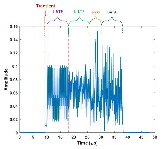
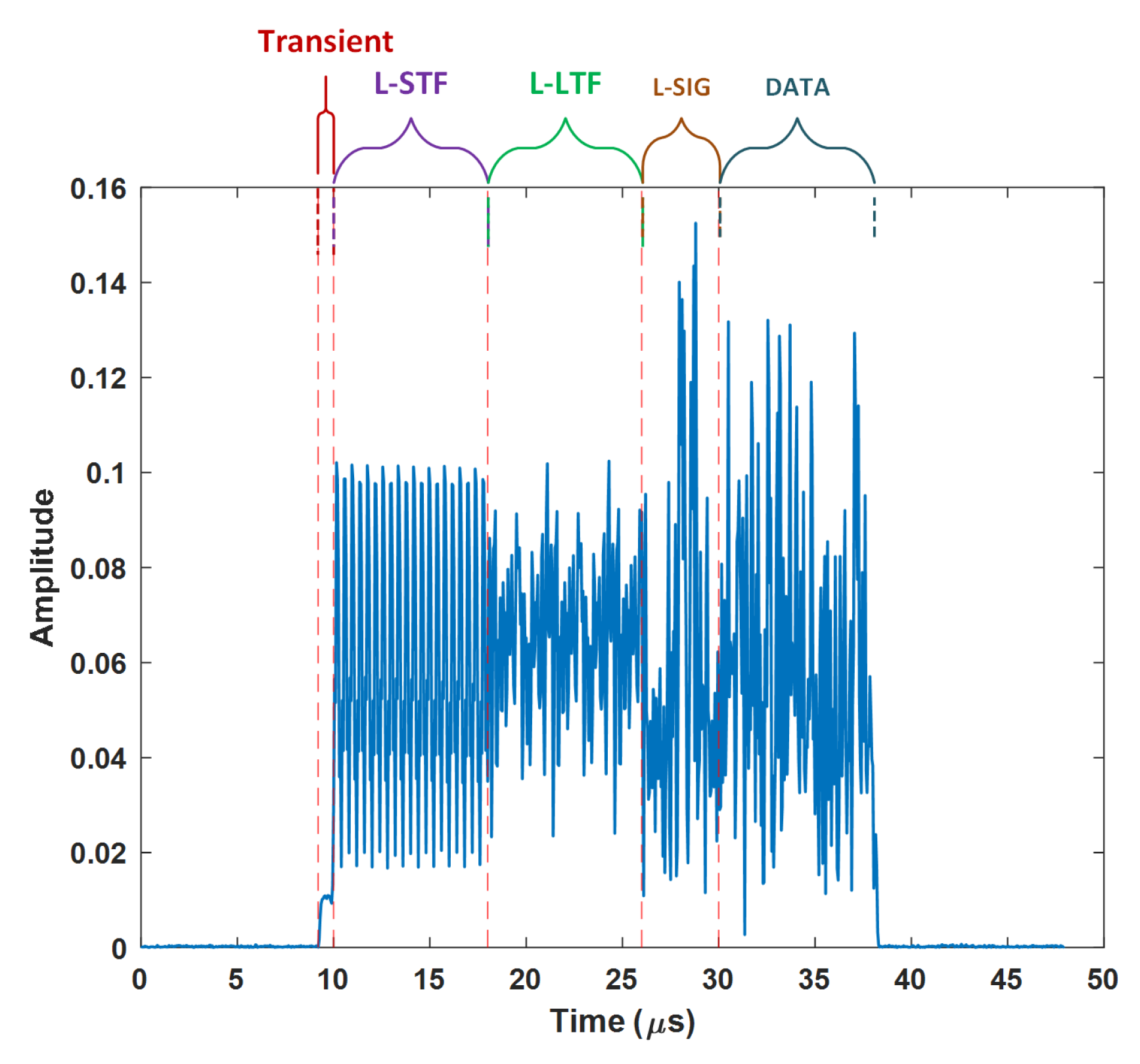
Legacy IEEE 802.11n [19] (non-high-throughput) Wi-Fi signals were used to test the overall performance of the proposed network. These signals are made up of three main parts: transients, preamble, and data. Transient signals emitted during power-on cycles can be used for device identification, as they exhibit unique unintended characteristics of transmitters [4]. The preamble part enables the receiver to perform certain operations, such as time synchronization, frequency offset compensation, and channel equalization. This part comprises the legacy short training field (L-STF, 2x OFDM symbols), the legacy long training field (L-LTF, 2x OFDM symbols), and the legacy signal field (L-SIG, 1x OFDM symbol). The data part of the 802.11n frame contains the service, payload (MAC layer data), tail, and pad bits.

In Figure 1, the transient and preamble parts of a captured 802.11n legacy frame can be observed. Since L-SIG and data parts contain payload-related information, these were not included in the scope of this study. In other words, raw I/Q signals containing transient, L-STF and L-LTF parts were used as input to the designed RF fingerprinting algorithm.

Figure 1. A legacy 802.11n signal packet.

In the next sections, detection and preprocessing of these signals will be discussed, respectively.

2.2. Signal Detection

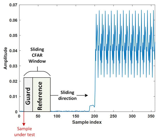
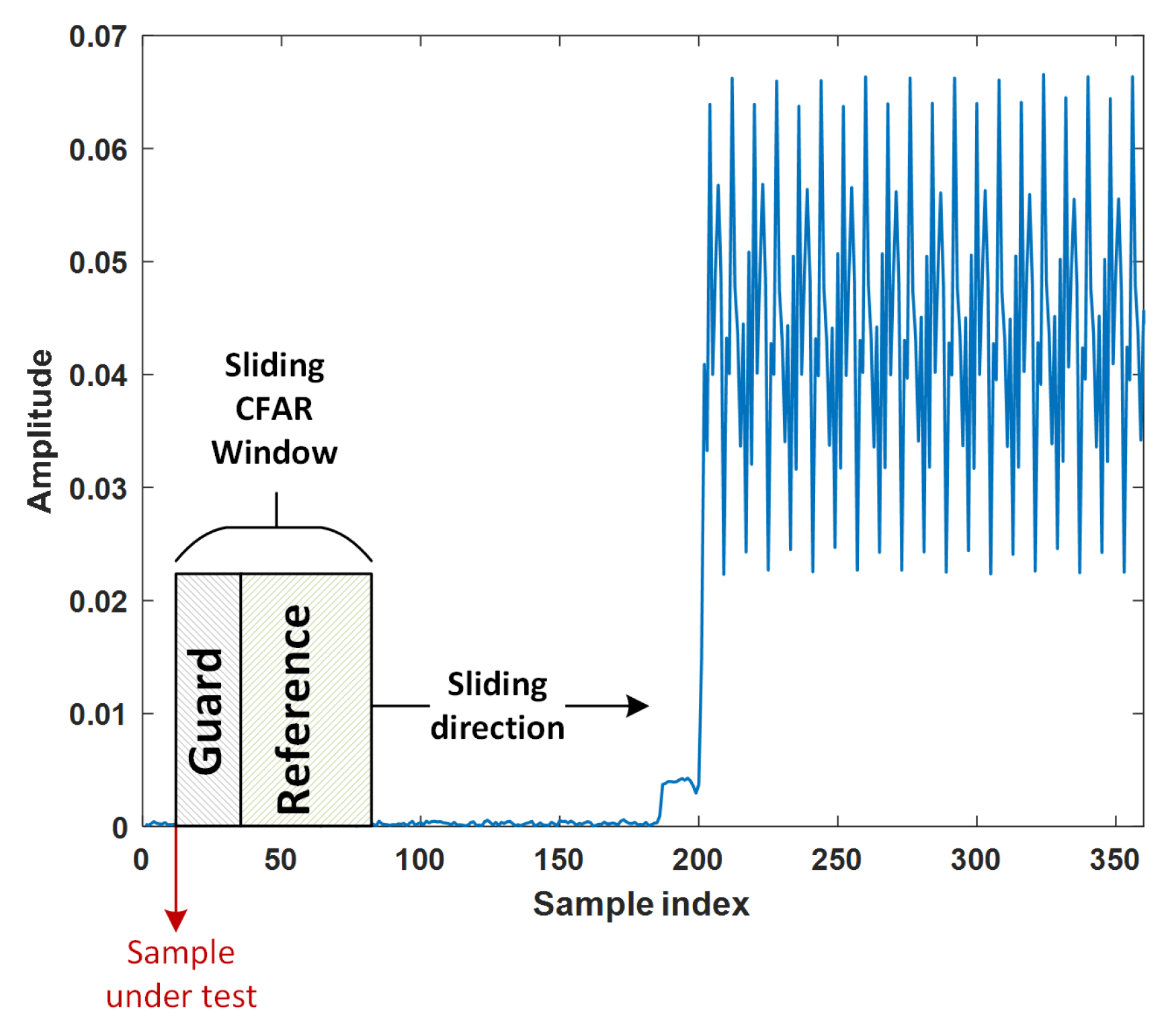
For transient signal detection, the constant false alarm rate (CFAR) detection algorithm is employed. CFAR detectors are adaptive types of Neyman–Pearson detectors that estimate the noise floor and maintain the false alarm rate at a constant level [20]. For the proposed CFAR detector, as shown in Figure 2, the sliding test window is on the leading side of the sample under test (also called the cell under test or candidate) to detect a transient starting point. The reference window is used to estimate the local noise level that is set as a threshold, while the instantaneous energy of the samples within the guard window is not used. Guard windows disable false detections due to abrupt energy leakage of the sample under test.

Figure 2. CFAR detector for transient detection.

The energy accumulated within the CFAR window can be written as follows:

$$E_{test}\left[n\right]=\sum _{k=1}^{N_{test}}{\left|x[n+k]\right|}^2,$$

(1)

where $x\left[n\right]$ is the received signal, $N_{test}$ is the length of the CFAR window, and n is the sample under test. The local noise power is estimated from reference window (with a length $N_{ref}$) samples as

$${\widehat{\sigma }}_n^2={\displaystyle \frac{1}{N_{ref}}}\sum _{i=N_{guard}+1}^{N_{test}}{\left|x[n+i]\right|}^2,$$

(2)

where $N_{guard}$ is the length of the guard window. The CFAR constant, $\alpha$, and the noise power estimate set the detection threshold as $T=\alpha ·{\widehat{\sigma }}_n^2$. $\alpha$ is determined with the desired probability of false alarm, $P_{FA}$, assuming that the null hypothesis (noise only) has a Chi-squared energy distribution [21]:

$$\alpha =[P_{FA}^{-1/N_{ref}}-1].$$

(3)

After that, if the total energy within the CFAR window is above the set threshold $E_{test}>T$, signal detection is achieved. In this study, $P_{FA}$ is set to 0.001.

The starting point of the preamble of the received 802.11n frame is detected by the wlanPacketDetect function of MATLAB (version R2024b) [22,23]. The function first performs the autocorrelation operation between the received signal, $x\left[n\right]$, and its delayed version $x[n+d]$:

$$R\left(\tau \right)=\sum _{n=0}^{d-1}x[n+\tau ]·x^{\ast }[n+d+\tau ],$$

(4)

where d corresponds to the number of delayed samples. Then, the function performs the autocorrelation operation of the delayed signal, $x[n+d]$:

$$E\left(\tau \right)=\sum _{n=0}^{d-1}{\left|x[n+d+\tau ]\right|}^2.$$

(5)

The method then applies normalization as follows:

$$R_{norm}\left(\tau \right)={\displaystyle \frac{{\left|R\left(\tau \right)\right|}^2}{E{\left(\tau \right)}^2}}.$$

(6)

The obtained decision statistics are then passed through a built-in threshold value. The first point that exceeds the threshold value is specified as the starting point of the preamble.

2.3. Preprocessing

The legacy 802.11n preamble parts include OFDM symbols for which the reference frequency should be the same for both transmission and reception operations. The carrier frequency offset (CFO) may occur due to hardware (master clock, local oscillator, etc.) imperfections that may result in asynchronous (mismatched) frequencies between transmitters and receivers. Uncompensated CFO may lead to the Doppler shift effect and inter-carrier interference [24], resulting in degraded RF fingerprinting performance. After extraction of transients and preamble parts, in order to eliminate the effect of CFO, coarse and fine CFO compensation are carried out. For this purpose, first, the L-STF signal part is extracted from the preamble and a coarse carrier frequency offset estimation is performed using the function wlanCoarseCFOEstimate [25]. The function first removes the cyclic prefixes of two OFDM symbols within the L-STF signal. After that, the phase information is extracted from the autocorrelation between the remaining signal and its delayed version of 16 samples. Finally, the obtained value is scaled and the coarse frequency offset estimation is completed.

The suppression of the estimated coarse frequency offset ($\Delta f_c$) is carried out as in the equation given below:

$$x_c=x·e^{-i2\pi \Delta f_{c}t}.$$

(7)

In the next step, the packet start time is fine-tuned using the wlanSymbolTimingEstimate function [26]. In this function, a cross-correlation is performed between the theoretically expected L-LTF signal and the received signal in which the coarse frequency offset is suppressed. According to this correlation result, the L-LTF start time is determined and, thus, the packet start time is updated. Later, a fine CFO estimate is obtained by using the function wlanFineCFOEstimate [27]. Conceptually, the fine frequency offset estimation is similar to the coarse frequency offset estimation, except that this time only L-LTF samples are used. The suppression of the estimated fine frequency offset, $\Delta f_f$, is performed as follows:

$$x_f=x_c{e}^{-i2\pi \Delta f_{f}t}.$$

(8)

In addition to CFO compensation, power normalization is applied per captured frame to eliminate device disentanglement due to power fluctuations [28,29]. The normalized waveform $x_{norm}$ is

$$x_{norm}={\displaystyle \frac{x}{\sqrt{\frac{1}{N}{\sum }_{n=0}^N{\left|x\right[n\left]\right|}^2}}}.$$

(9)

For notational simplicity, the power-normalized received signal $x_{norm}$ is denoted as x in the following sections.

3. Classifier Structure

Since raw I/Q samples are used as RFFs, the classifier structure must be adapted to handle complex values. In this work, the classifier network is configured based on complex convolutional layers and activation units. First, the convolutional neural network (CNN) model is evaluated to establish a supervised baseline. Then, this architecture is extended to explicitly disentangle device-specific and channel-dependent features by employing adversarial and triplet losses.

3.1. Complex-Valued Convolutional Neural Network

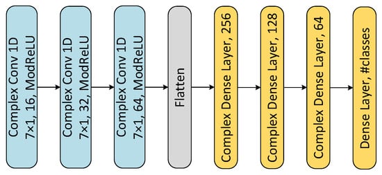
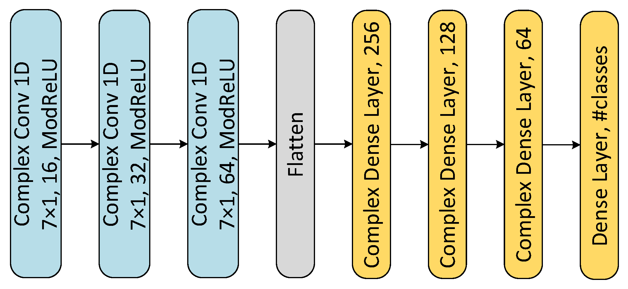
In this study, one-dimensional complex-valued convolutional neural networks (CVCNNs) are employed to better extract local characteristics. Generally, raw I/Q samples are fed into a network with two channels as real (in-phase) and imaginary (quadrature) parts. However, in this case, functions like convolutions and activations within a network are generally applied to real and imaginary parts separately. In this study, the designed CVCNN provides complex convolution operations and complex activation functions that are directly applied to the raw I/Q sample within a single channel. The architectural structure for the CVCNN is demonstrated in Figure 3.

Figure 3. The proposed one-dimensional complex-valued CNN.

ComplexConv1D is a complex convolutional layer that contains kernels (filters) with a response $h\left[n\right]$. Assuming that the received and preprocessed I/Q signal is $x\left[n\right]$, the complex convolution of $x\left[n\right]$ and $h\left[n\right]$ can be written as follows:

$$\begin{array}{cc}\hfill y\left[n\right]& =\sum _{k}x[n-k]h\left[k\right],\hfill \\ \hfill y\left[n\right]& =\sum _k(x_r[n-k]+j{x}_i[n-k])(h_r\left[k\right]+j{h}_i\left[k\right]),\hfill \\ \hfill y& =(x_r\ast h_r-x_i\ast h_i)+j(x_r\ast h_i+x_i\ast h_r),\hfill \end{array}$$

(10)

where ∗ denotes the convolution operation, n is the index of the output sample being calculated, and k represents the coefficient index that spans the kernel length.

In addition, modReLU activation layers are utilized in the CVCNN network. The formula for this activation function is as follows:

$$f\left(z\right)=ReLU\left(\right|z|+b)·{\displaystyle \frac{z}{\left|z\right|}},$$

(11)

where $b\in R$ is a nonlinearity bias parameter. Hence, the activation function applies a magnitude threshold while maintaining the phase of complex data [30]. Standard CNN structures with two channels (I and Q) without weight constraints might not preserve the phase information of the received signal [31,32].

3.2. TripletDANN and Loss Functions

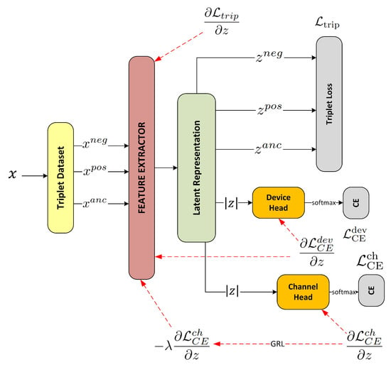
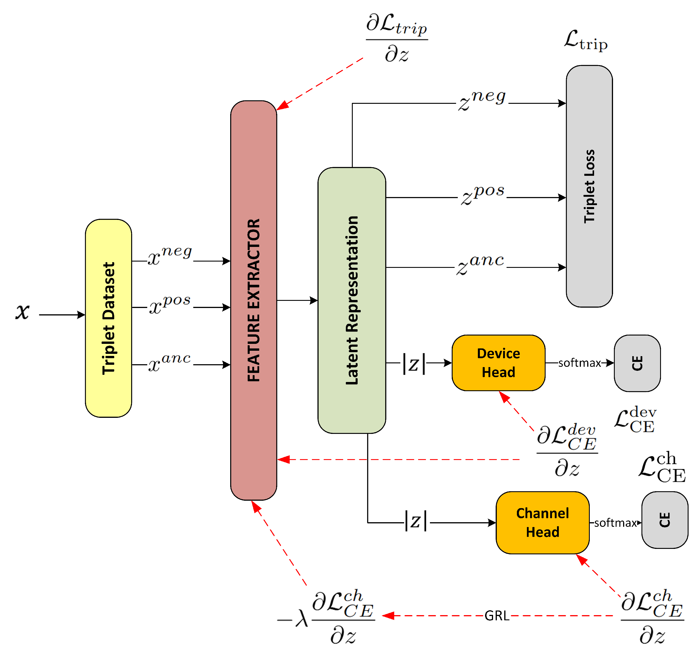
In this work, the complex-valued convolutional neural network is mainly employed as an autonomous feature extractor from raw I/Q samples. After feature extraction, the latent space feature vector is fed into the device head and channel head, which comprise multilayer perceptrons (MLPs). The device head and channel head yield a softmax output according to the device and channel labels. To improve the robustness of the model, adversarial loss is utilized in a manner similar to that provided by domain-adversarial neural networks (DANNs). This type of network is generally used to adapt feature spaces in different domains [33]. In addition to adversarial loss, the triplet loss is also incorporated into the total loss function to further enhance the model’s resilience against channel variations. Consequently, the TripletDANN architecture is introduced as in Figure 4. The calculations of the loss function and the gradient flow during backpropagation are also demonstrated in this figure.

Figure 4. Proposed TripletDANN architecture.

The proposed TripletDANN comprises a feature extractor, a device head, and a channel head. The feature extractor, structured as a CVCNN without an output layer, outputs the latent space vector z, which is then fed into the channel and device heads.

The device head is formed to enable the identification of devices. It consists of a single fully connected layer (64 → $N_{DEV}:15$), which produces device logits from the learned latent embeddings. In the training loop, the cross-entropy loss ($CE$) is computed from the softmax output of the device head.

Similarly, the channel head is configured as a fully connected neural network to classify the channel of the devices according to the assigned channel labels. The channel head consists of batch normalization followed by a two-layer multilayer perceptron (64 → 256 → $N_{ch}$) that produces channel logits. Cross-entropy loss is used for the loss function of the channel head.

In addition to cross-entropy losses of device and channel heads, the triplet loss derived from latent features is computed and added to the total loss function. Triplets are generated using sampling over the entire dataset rather than by mining within a batch. Each triplet is independently created by drawing an anchor, a positive, and a negative example from the full dataset, and batches are formed by grouping these independently sampled triplets. A comparatively large batch size (512) is used to keep the proportions of anchors, positives, and negatives well balanced. No hard negative mining strategy is applied. The anchor set is composed of data from every device and channel label present in the training dataset. The positive subset is formed by concatenating data samples originating from the same device in different channels, while the negative subset contains data samples from different devices. Assume, for example, that in a single batch anchor the first sample consists of data labeled device $\#01$, channel $\#02$. For this case, the positive sample might be from data labeled device $\#01$, channel $\#05$, while the negative sample may be from data labeled device $\#04$, channel $\#02$. The network is enforced to focus solely on device-specific latent features by feeding a triplet dataset, ensuring that these features are generalized across different channels. Triplet loss is obtained from latent features using the $L_2$ norm as follows:

$${\mathcal{L}}_{\mathrm{trip}}=\sum _i^N[\parallel z_i^{anc}-z_i^{pos}{\parallel }_2^2-\parallel z_i^{anc}-z_i^{neg}{\parallel }_2^2+\mu ],$$

(12)

where $z^{anc}$, $z^{pos}$, and $z^{neg}$ are latent vectors obtained from the anchor set, the positive subset, and the negative subset samples, respectively [15,16]. A margin parameter $\mu$ ensures that the distance between $z^{anc}$ and $z^{pos}$ in the latent space is at least $\mu$ smaller than the distance between $z^{anc}$ and $z^{neg}$ [34]. Thus, $z^{anc}$ is pushed towards $z^{pos}$ instead of $z^{neg}$ in the feature space. Training starts with a forward pass: the feature extractor generates a latent vector z, which is then fed into the device head and the channel head. The triplet loss is computed based on the distance of the anchor’s latent embeddings with respect to the latent features of positive and negative subsets, whereas the cross-entropy losses are calculated on the basis of channel and device predictions. Then, the total loss function is calculated as follows:

$$\begin{array}{cc}\hfill L& ={\kappa }_{dev}·{\mathcal{L}}_{\mathrm{CE}}^{\mathrm{dev}}+{\kappa }_{ch}·{\mathcal{L}}_{\mathrm{CE}}^{\mathrm{ch}}+{\kappa }_{trip}·{\mathcal{L}}_{\mathrm{trip}},\hfill \end{array}$$

(13)

where ${\kappa }_{dev}$, ${\kappa }_{ch}$, and ${\kappa }_{trip}$ are weighting coefficients of the corresponding losses. All hyperparameters, including the loss weighting coefficients and the triplet margin, were determined through empirical tuning based on extensive preliminary experiments. Multiple configurations were evaluated using validation performance as the primary criterion to ensure stable convergence and balanced contributions from competing loss components. The final values of ${\kappa }_{\mathrm{dev}}=1.0$, ${\kappa }_{\mathrm{ch}}=0.5$, ${\kappa }_{\mathrm{trip}}=1.0$, and the triplet margin $\mu =1$ correspond to near-optimal settings, and no significant performance improvement was observed beyond these configurations.

Subsequently, during the backpropagation of TripletDANN, the channel head and device head parameters are updated to minimize their respective losses ${\mathcal{L}}_{\mathrm{CE}}^{\mathrm{chan}}$ and ${\mathcal{L}}_{\mathrm{CE}}^{\mathrm{dev}}$. In contrast, the parameters of the feature extractor are optimized using the gradient of ${\mathcal{L}}_{\mathrm{CE}}^{\mathrm{dev}}$, ${\mathcal{L}}_{\mathrm{trip}}$ along with the reversed and scaled gradient of ${\mathcal{L}}_{\mathrm{CE}}^{\mathrm{chan}}$. This gradient inversion is performed by the gradient reversal layer (GRL), originally introduced in [35]. The GRL acts as an identity mapping during the forward pass, while enabling adversarial training by reversing and scaling the gradient of the channel classification loss during the backpropagation. Mathematically, the GRL operation for the feature extractor can be defined as follows:

$${\mathrm{GRL}}_{\lambda }\left(z\right)=\left\{\begin{array}{cc}z,\hfill & \mathrm{forward}\mathrm{propagation},\hfill \\ -{\lambda }_{grl}{\displaystyle \frac{\partial {\mathcal{L}}_{CE}^{ch}}{\partial z}},\hfill & \mathrm{backpropagation}.\hfill \end{array}\right.$$

(14)

where ${\lambda }_{grl}$ is the weighting of GRL. Ganin suggested a schedule for ${\lambda }_{grl}$ so that it remains zero from epoch 1 to epoch 5, after which it gradually increases to 1 [35]:

$${\lambda }_{grl}\left(epoch\right)=\left\{\begin{array}{cc}0,\hfill & \mathrm{epoch}\le 5,\hfill \\ {\displaystyle \frac{2}{1+e^{-10\frac{(epoch-5)}{(total\#ofepochs-5)}}}}-1,\hfill & \mathrm{epoch}>5.\hfill \end{array}\right.$$

(15)

Alternatively, another scheduling named ramp-down is suggested. The network is subjected to high adversarial loss at epoch $\#5$ and then stabilized by setting ${\lambda }_{grl}$ to $0.4$ at the end of training:

$${\lambda }_{grl}\left(epoch\right)=\left\{\begin{array}{cc}0,\hfill & \mathrm{epoch}\le 5,\hfill \\ 1-0.6{\displaystyle \frac{epoch-5}{total\#ofepochs-5}},\hfill & \mathrm{epoch}>5.\hfill \end{array}\right.$$

(16)

The general flow chart of the gradients computed during the backward pass of the TripletDANN training can be seen in red dashed lines in Figure 4. In the training phase, device MAC addresses are used as labels for the device head, whereas assigned channel labels are used to obtain the triplet dataset and to supervise the channel head. Channel labels are excluded during the evaluation phase.

4. Experimental Setup

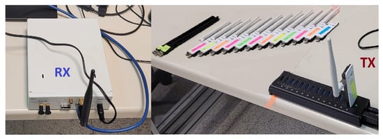
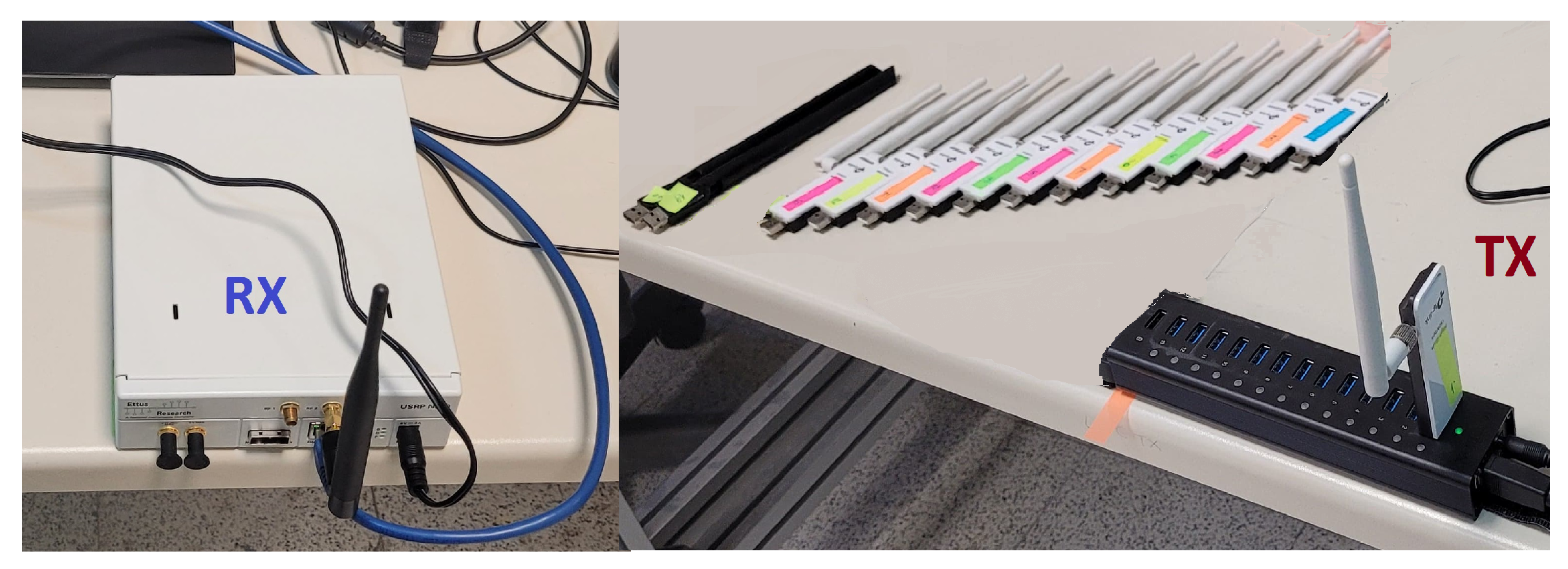
The devices to be identified are Wi-Fi adapters that comply with the IEEE 802.11n legacy mode. The total number of Wi-Fi devices is 15 ($13\times$ TP-Link Wireless USB Adapter and $2\times$ Realtek 8811CU Wireless LAN 802.11ac USB NIC). An access point establishes a connection with wireless devices, enabling the devices to transmit Wi-Fi signals. The USRP N210 software-defined radio equipped with an UBX-40 RF daughterboard is used as a receiver, as shown in Figure 5.

Figure 5. Transmitting Wi-Fi devices and the receiver.

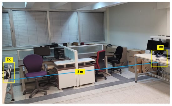
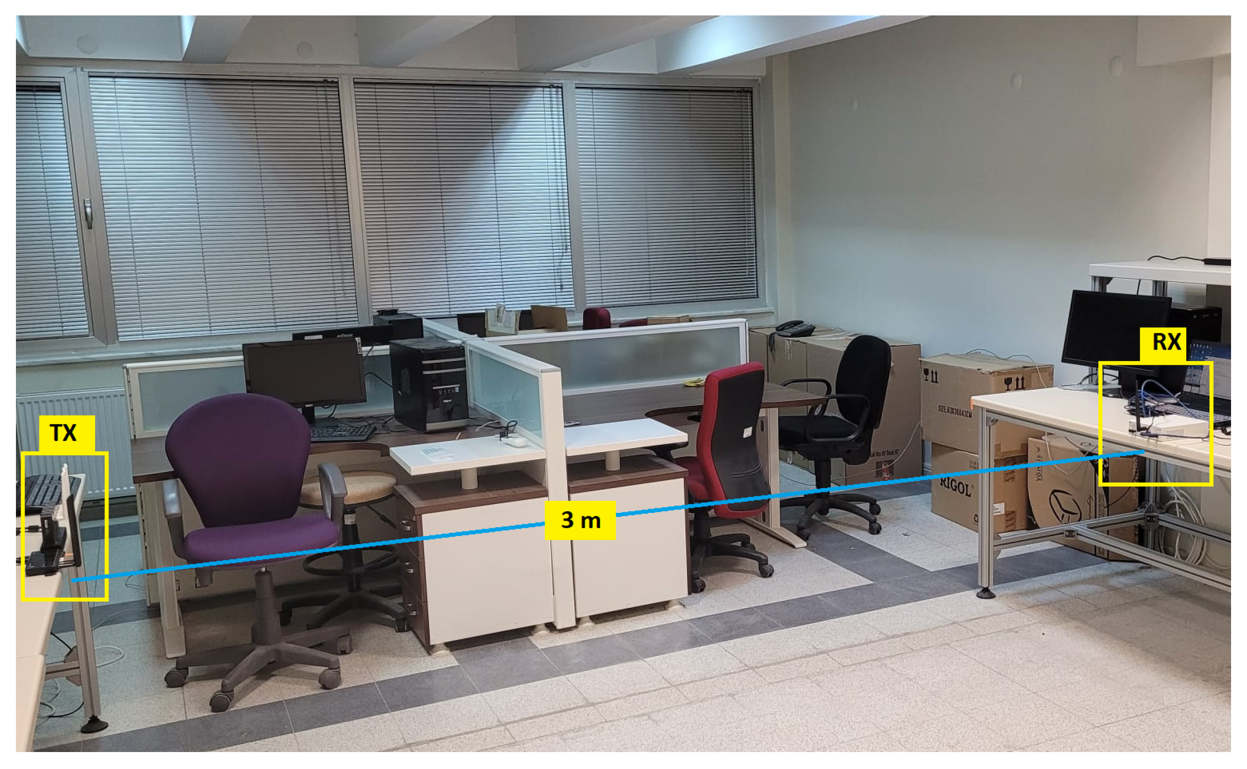
The Wi-Fi signals were captured with a sampling rate of 20 MSa/s. After demodulation, the captured Wi-Fi packets were saved and labeled according to their MAC addresses. In Figure 6, the experimental setup is demonstrated, in which the transmitters and the receiver are approximately three meters apart.

Figure 6. Experimental setup in the laboratory.

For experiments, the transmitting devices were placed either at a single fixed location or at multiple fixed locations, while the receiver was placed in different locations. The experiments were conducted under static environmental conditions on different days. A TX–RX separation of approximately 3 m was maintained to ensure far-field conditions. Data were collected at receiver locations spaced 30 cm apart, with both TX and RX placed on 1 m high tables. Despite the presence of many scattering objects in the laboratory, the propagation environment was predominantly line-of-sight (LOS). In some cases, the antennas of the transmitting devices could partially obstruct the direct LOS paths of other transmitters. For each device, 1000 Wi-Fi packets were collected in less than 3 min.

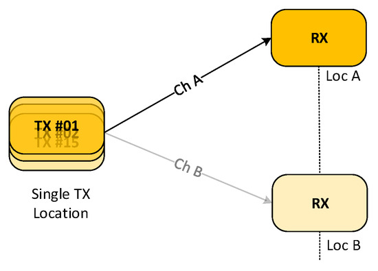
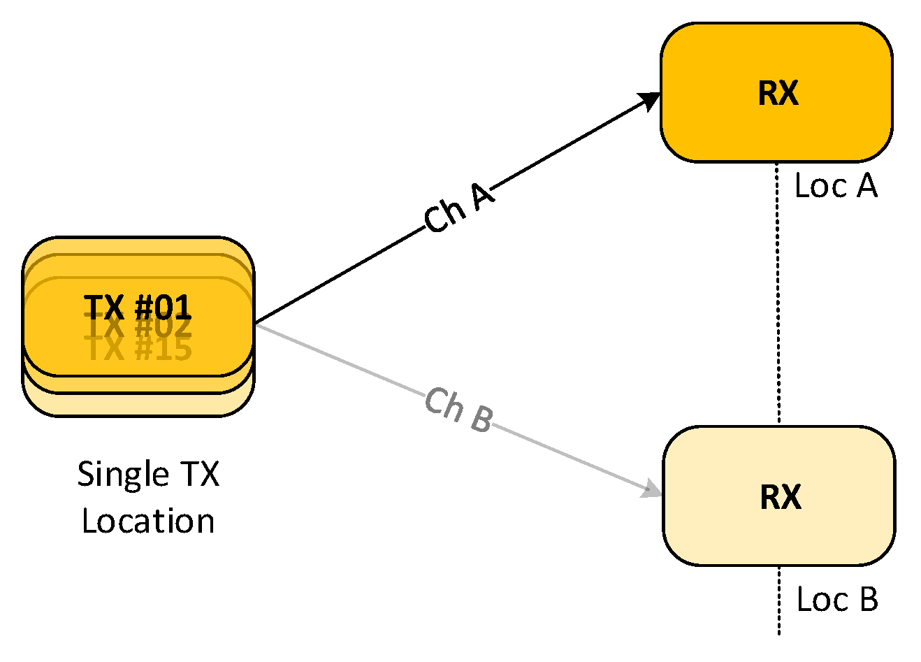
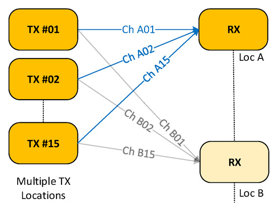
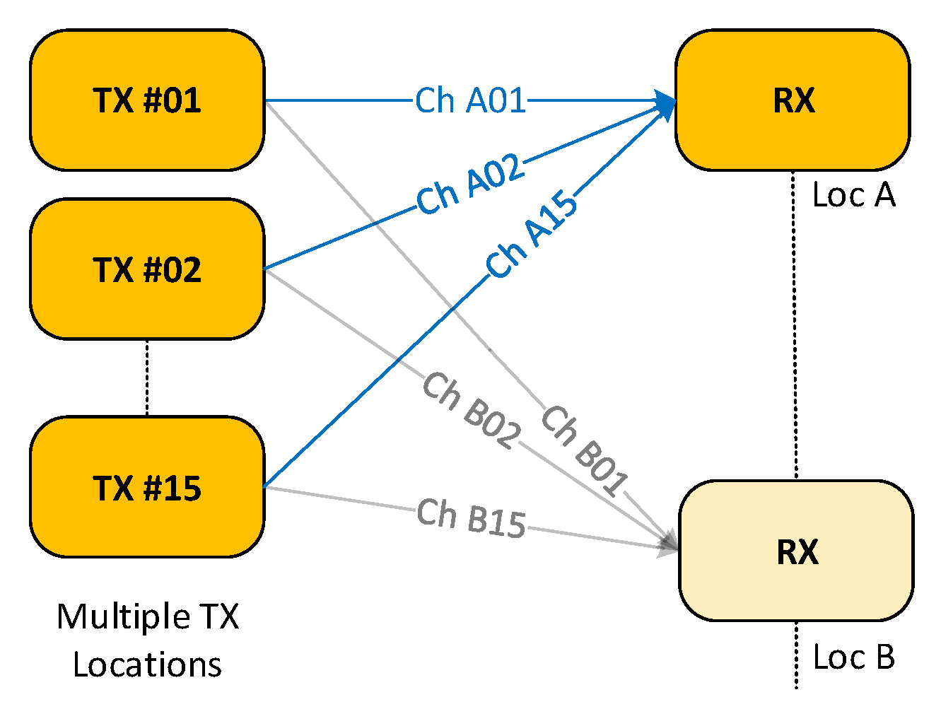
In the experiments, two types of data collection scenarios were considered, namely SL (single-location) and ML (multi-location). In the SL scenario, the transmitters were placed at a single fixed position, whereas in the ML scenario, they were deployed at multiple distinct and fixed locations. The data gathered in Scenario ML is regarded as more realistic and challenging for deriving channel-robust RF fingerprints since TX devices may be spatially distributed across different locations in practice. For each scenario, the receiver was placed in different locations. Data collection scenarios are illustrated in Figure 7 and Figure 8.

Figure 7. SL data collection scenario.

Figure 8. ML data collection scenario.

For Scenario SL, transmitters were placed at a fixed location, whereas the receiver location was changed after capturing 1000 packets from all transmitters (TX #1–#15). Channel labeling of data was performed according to the location of the receiver in this scenario. For example, the data collected at receiver location A was labeled as Channel A (Ch A). Similarly, the data collected at receiver location B was labeled as Channel B (Ch B), and the data for subsequent receiver locations were labeled accordingly.

For Scenario ML, the transmitters were placed at multiple distinct locations. The receiver location was changed once the packets from all transmitters were captured, as in Scenario SL. Data labeling was carried out based on the locations of the transmitters and the receiver for Scenario ML. For example, at receiver position A, channel labels were assigned to each transmitter data individually, i.e., Ch A01 to Ch A15. Data from subsequent receiver locations were labeled in the same manner. Hence, the positive subsets of the triplet dataset were modified to enable fine-grained supervision. An example of channel labeling is presented for two receiver locations in Table 1.

Table 1. Channel labeling applied in training.

Scenarios	RX Location	Channel Labels
SL	A	Ch A
ML	A	Ch A01–Ch A15
SL	B	Ch B
ML	B	Ch B01–Ch B15

5. Training Strategies

TripletDANN achieves channel robustness by taking advantage of triplet loss and adverserial training through the aggregation of data with at least two different channel labels. This is motivated by the insight that data collected from a single RX location may not provide enough representation of channel-specific data to the feature extractor, so the network may not separate channel- and device-specific features from each other. Two different data expansion approaches were employed: the first was aggregation of data collected at different receiver locations, while the second was the application of data augmentation techniques.

Data aggregation is performed by combining each observation per device from different channels. For this purpose, 800 observations per device collected from at least two different RX positions are aggregated for the training dataset, while 200 observations per device are aggregated for the validation dataset. When collecting data from multiple receiver locations is not feasible or practical, TripletDANN can be used in conjunction with data augmentation. This enables generalization through channel simulations.

In this study, data collected from a single receiver location under static channel conditions, i.e., channel conditions slightly vary over the duration of data collection, were augmented by synthetic data. The data augmentation process is as follows.

• Data were collected from a fixed position of the receiver. Measurements were conducted under line-of-sight conditions [10].
• Since the laboratory environment corresponds to a large office scenario, the TGn Model-C can be appropriately utilized, as described in [36]. Therefore, TGn channels with Model-C were randomly generated and channels were stored [37].
• The collected signals were passed through the stored channels. For Scenario SL, the observations of all devices were passed through the same channels. For Scenario ML, the observations of each device were passed through different channels.
• Transient detection was performed, and delayed samples were circularly shifted so that they aligned with the original signal.
• Augmented data was saved and channel labels were assigned according to the type of scenario.

6. Results and Analysis

In this section, we present the experimental analysis and results. For testing, 1000 samples per device collected at unseen locations were used. The reported test results are obtained by training the models using five-fold cross-validation and averaging the results across the folds. We define two types of testing scenario, namely same-scenario and cross-scenario evaluations. The same-scenario evaluation means that both the training and test datasets are formed under the same data collection scenario, i.e., train in SL, test in SL or train in ML, test in ML ($SL\to SL$ or $ML\to ML$). The cross-scenario evaluation corresponds to training and test datasets being formed under different data collection scenarios, i.e., train in SL, test in ML or train in ML, test in SL ($SL\to ML$ or $ML\to SL$).

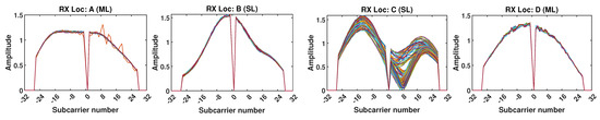
In order to visualize channel characteristics, sample channel estimates from the collected data are demonstrated in Figure 9. Channel estimates show that channels typically exhibit a moderate level of variation as the TX–RX geometry changes. Location- and scenario-dependent behavior as well as occasional quasi-static behavior of channels can be observed.

Figure 9. Channel estimates for device #14 across different locations and data collection scenarios.

6.1. Impact of the Number of RX Locations Used for Data Aggregation

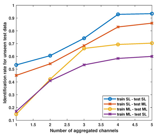
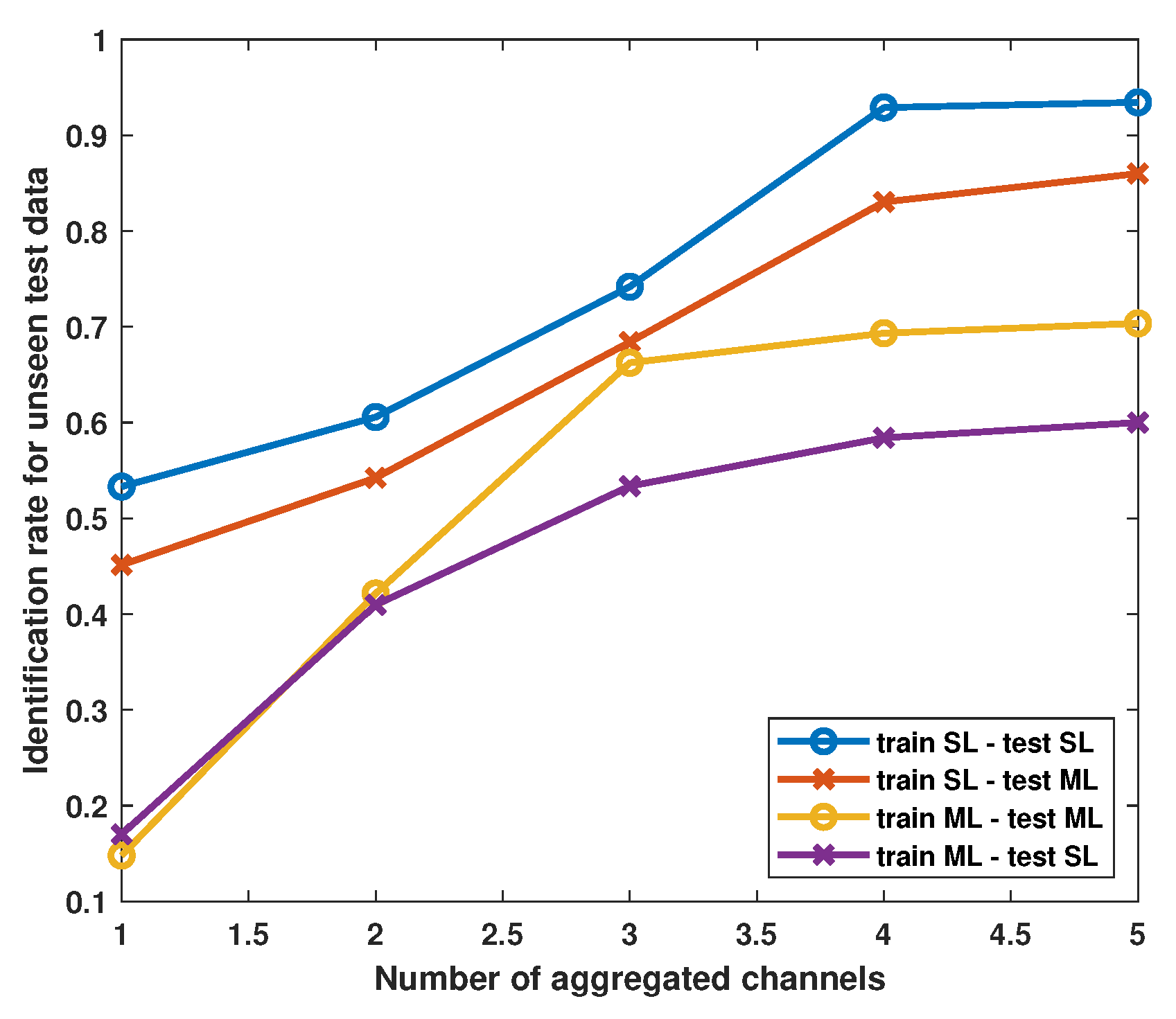
Before evaluating the TripletDANN model, the aggregation of data from different channels within each scenario is analyzed in Figure 10. Evidently, when the CVCNN is trained without data aggregation (i.e., data from only one channel) in the ML setup, it performs poorly in both same-scenario and cross-scenario evaluations. Training the network within the SL scenario improves test accuracy, particularly without relying on data aggregation. It can be deduced that the channel effects on the collected data across all devices tend to be largely similar. In addition, notice that increasing the aggregated data from different channels saturates the generalization, especially for ML scenarios. However, in general, data aggregation enhances the identification performance for all scenarios. This observation demonstrates that the data aggregation approach adopted by the proposed TripletDANN can improve performance across the same- and cross-test scenarios. Furthermore, we use domain adaptation techniques based on triplet and adversarial losses to enhance channel robustness even in the case of a limited number of datasets to be combined.

Figure 10. CVCNN test accuracies against the number of aggregated channels.

6.2. Compared Methods

The performance of the proposed TripletDANN model is evaluated against three other models using raw I/Q data: CVCNN, DANN, and TripletCNN. For a fair comparison, all models are trained using an identical batch size of 512 and the same number of epochs, specifically 35, as employed for TripletDANN. The AdamW optimizer with a learning rate of $0.001$ is used to train the models. CVCNN is the baseline model and consists solely of the feature extractor and the device head. The standard DANN model trained using the Ganin scheduling strategy [35] corresponds to the CVCNN architecture with an additional channel head. TripletCNN is the network that omits the channel head and relies on triplet loss instead.

In addition, to enable a direct comparison between the proposed method and a feature-based technique, we employ the channel-independent spectrogram (CIS) method described in [10]. Although this feature was originally developed for the LoRa protocol, we adopt the core principle of the method for the Wi-Fi protocol. For this purpose, we compute the short-time Fourier transform (STFT) of the preamble segment of the raw I/Q signals, employing a window length (equivalently, FFT size) of 64 samples and an overlap ratio of 0.75 between consecutive windows. After that CIS is obtained by

$$CIS=20lo{g}_{10}{\displaystyle \frac{\left|S\right(f,w\left)\right|}{\left|S\right(f,w-1\left)\right|}},$$

(17)

where f denotes frequency bins and w denotes the number of window bins of the spectrogram. The dimensionality of the CIS matrix is $64\times 16$. Then, we form a 2D real-valued CNN with the same layer and filter numbers as the CVCNN, except that, due to the small size of the columns of the CIS, we alter the kernel size from 7 to 3. The proposed model and the compared methods are summarized in Table 2.

Table 2. Model summary and training losses.

Model	Structure	Training Losses
CVCNN	Feature Extractor → Device Head	${\mathcal{L}}_{\mathrm{CE}}^{\mathrm{dev}}$
DANN	Feature Extractor → Device & Channel Heads	${\mathcal{L}}_{\mathrm{CE}}^{\mathrm{dev}},{\mathcal{L}}_{\mathrm{CE}}^{\mathrm{ch}}$
TripletCNN	Feature Extractor → Device Head	${\mathcal{L}}_{\mathrm{CE}}^{\mathrm{dev}},{\mathcal{L}}_{\mathrm{trip}}$
TripletDANN	Feature Extractor → Device & Channel Heads	${\mathcal{L}}_{\mathrm{CE}}^{\mathrm{dev}},{\mathcal{L}}_{\mathrm{CE}}^{\mathrm{ch}},{\mathcal{L}}_{\mathrm{trip}}$
CIS + CNN2D	Feature Extractor → Device Head	${\mathcal{L}}_{\mathrm{CE}}^{\mathrm{dev}}$

6.3. Performance Comparison Under Data Aggregation

To obtain a comparative performance evaluation between TripletDANN and the networks given in Table 2, the datasets captured from different RX locations within the SL and ML scenarios were aggregated.

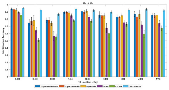
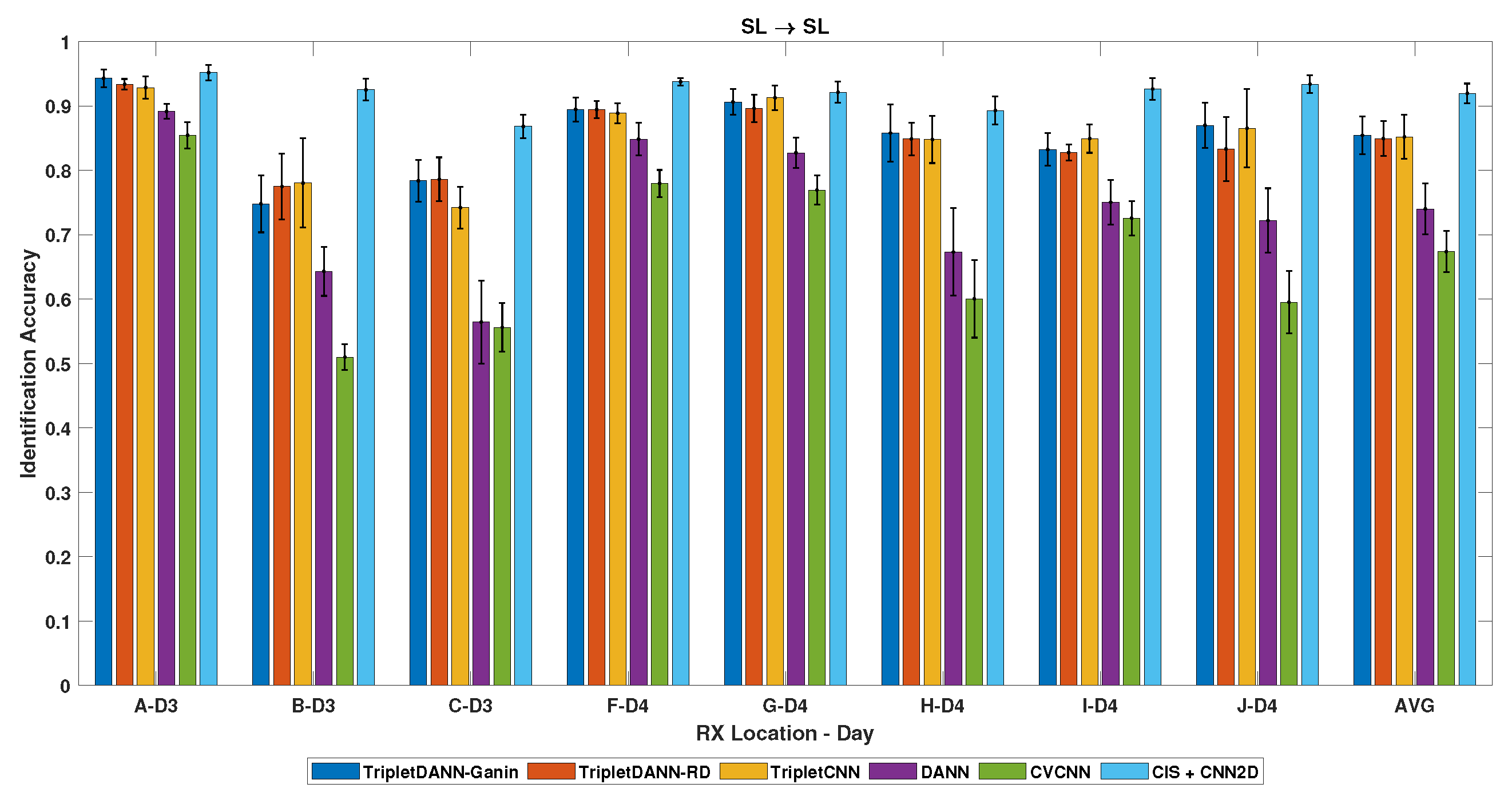
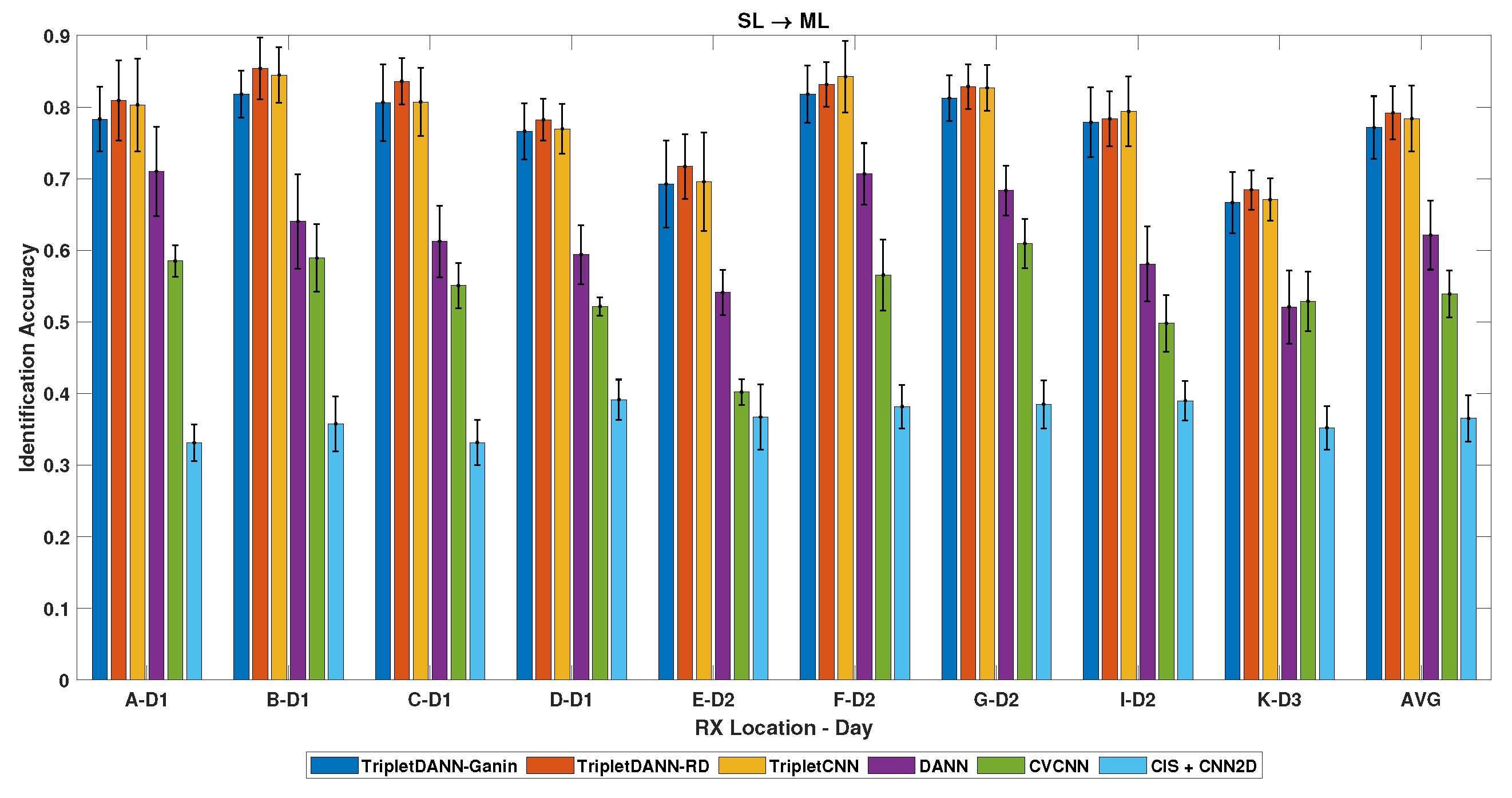
Firstly, we evaluated the performance of the networks at different RX positions in the SL data collection scenario. For this purpose, we combined the data collected from receiver locations D and E. The performance of Triplet DANN trained with ramp-down (RD) and Ganin scheduling (see Section 3) and the other models for this case study were compared within the same- and cross-scenario evaluations. In the same-scenario evaluation ($SL\to SL$), TripletDANN and TripletCNN outperform standard DANN and CVCNN, achieving an average test accuracy of around $85\%$, as shown in Figure 11. The CIS feature exhibits the highest performance in the same-scenario evaluation. In addition, error bars are shown to reflect the variation in accuracy across folds, corresponding to one standard deviation. In the cross-scenario evaluation ($SL\to ML$), TripletDANN achieves an average test accuracy of about $78\%$ and the highest test accuracy of $85.39\%$, as demonstrated in Figure 12. The identification performance of the CIS feature with the CNN2D network drastically drops to an average of $36.5\%$.

Figure 11. Identification results across unseen channels—train: SL, test: SL (same-scenario).

Figure 12. Identification results across unseen channels—train: SL, test: ML (cross-scenario).

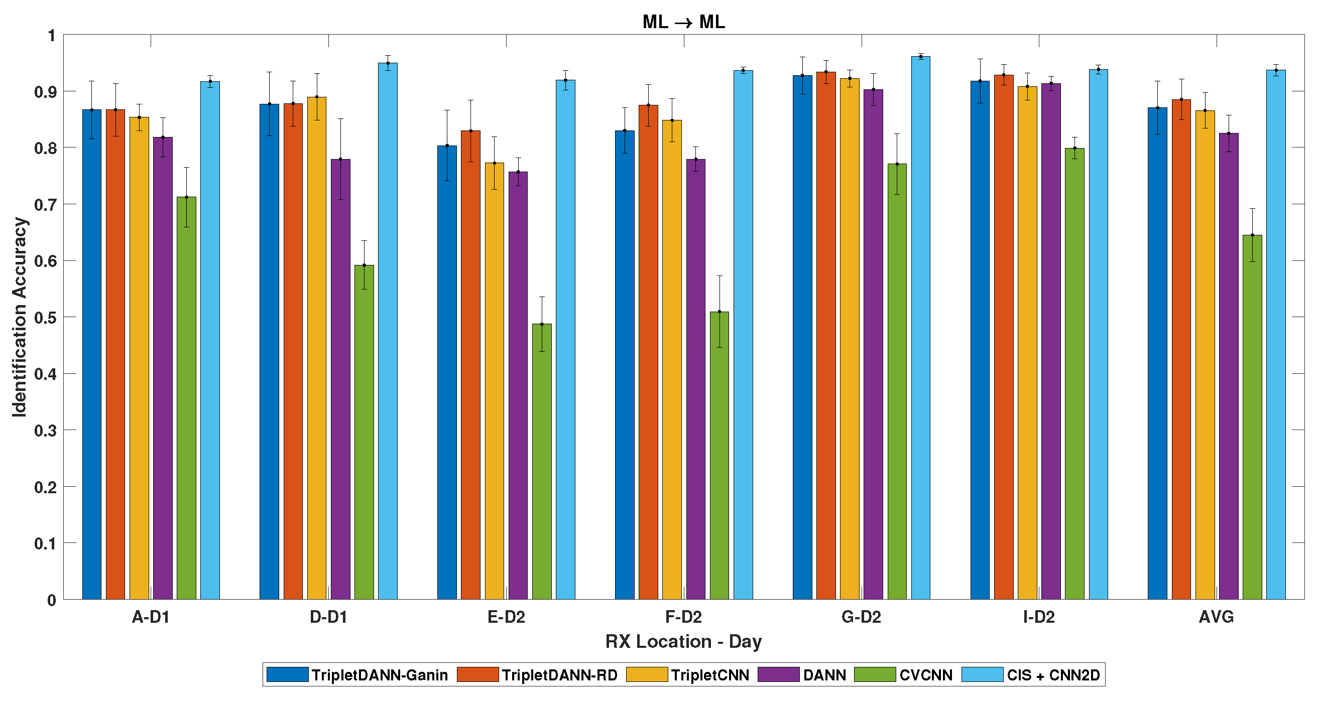
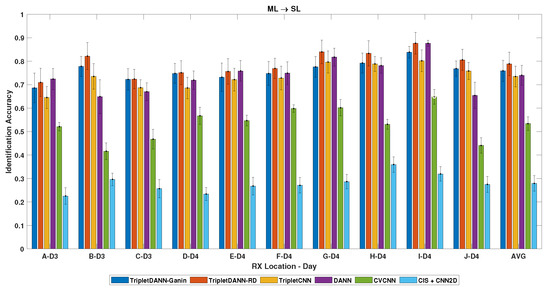
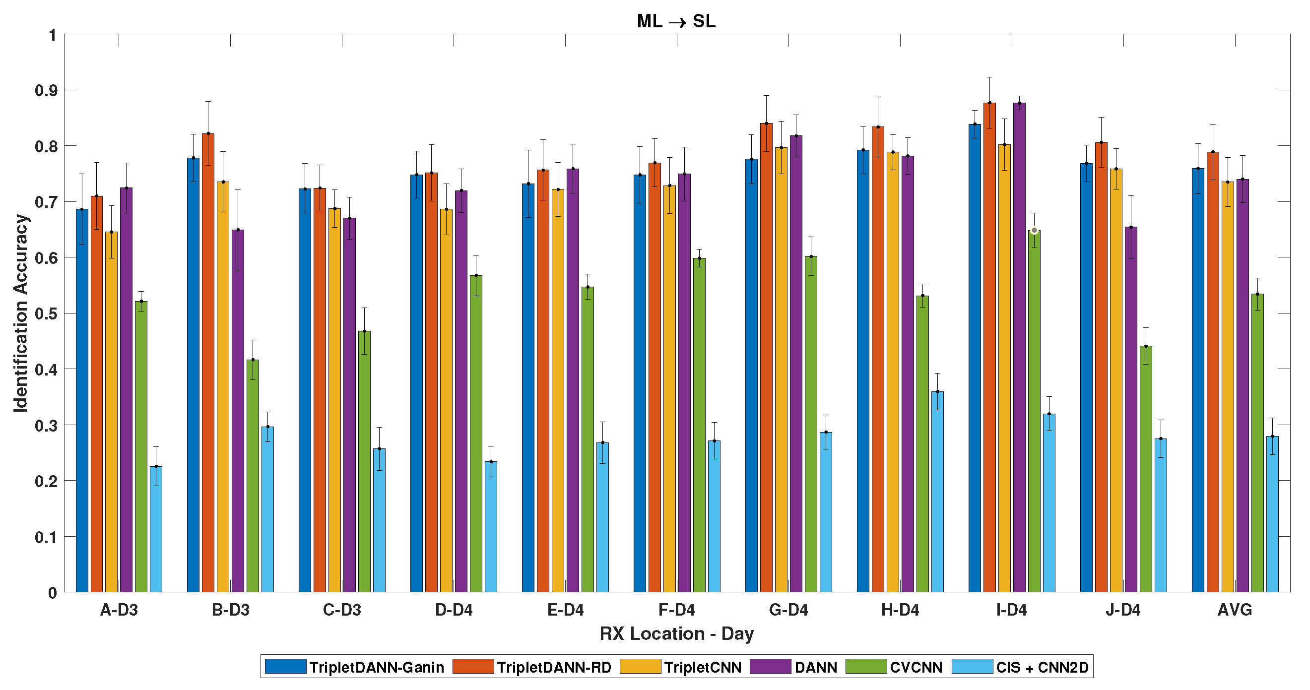
Secondly, we investigated the device classification performance of the networks in the ML data collection scenario. Network training is performed with a dataset that was aggregated from data collected in the B, C, and K channels in the ML setup. In Figure 13, TripletDANN employing the ramp-down schedule demonstrates the highest average accuracy of $88.52\%$ among the models using raw I/Q inputs under same-scenario evaluation ($ML\to ML$). The feature-based CIS method achieves the highest average classification accuracy, outperforming raw I/Q signal-driven networks. In cross-scenario tests ($ML\to SL$), TripletDANN with ramp-down scheduling once again achieves the highest average accuracy, reaching $78.88\%$ across ten unseen RX locations, as shown in Figure 14. TripletDANN outperforms TripletCNN, achieving an average gain of about $5\%$ and a $14\%$ improvement in Ch B data. The CIS method exhibits the lowest average accuracy among all methods in cross-scenario evaluations.

Figure 13. Identification results across channels—train: ML, test: ML (same-scenario).

Figure 14. Identification results across unseen channels—train: ML, test: SL (cross-scenario).

To provide further insight into the channel robustness of the proposed method, CVCNN is adopted as a reference model because it does not include any dedicated channel robustness mechanism. CVCNN exhibits varying average accuracies across different RX locations. This suggests that under same-scenario evaluation, CVCNN can achieve a reasonable level of accuracy when the test channel conditions are relatively similar to those observed during training (e.g., ML→ML, locations G and I). However, when such similarity diminishes (e.g., ML→ML, locations D and E), the performance of CVCNN degrades substantially. In contrast, under the same conditions TripletDANN outperforms CVCNN by up to 33.74% (see Figure 13). Therefore, the results indicate that the proposed method maintains robust performance under channel variations arising from changes in TX–RX geometry.

Overall, the proposed TripletDANN method achieves consistently strong identification performance in all evaluated test scenarios. In same-scenario evaluations, it generally achieves higher accuracy than approaches based on raw I/Q input, while its performance remains comparable to the feature-based method, with a modest performance gap. In cross-scenario evaluation, TripletDANN outperforms all compared methods, indicating strong generalization capability. Additionally, the error bars indicate that the proposed method demonstrates consistent performance for all evaluation scenarios. The standard deviation values are generally comparable to those of the compared methods, except in the same-scenario evaluation case where CIS shows lower variability.

The literature frequently discusses computational complexity, the size of network parameters, and the efficiency of inference [38,39]. For all methods given in Table 2, the computational performance analysis is presented in Table 3. All models were trained and tested on an NVIDIA GeForce RTX 3050 Ti GPU using CUDA 12.8.

Table 3. Comparison of model complexity and inference time.

Model	Input	Number of Parameters (M)	Average Batch Latency (ms)	Inference Time per Sample (µs)
CNN2D	CIS	0.164	1.89	3.75
CVCNN	Raw I/Q	0.390	6.82	13.6
DANN	Raw I/Q	0.407	7.10	14.0
TripletCNN	Raw I/Q	0.390	6.60	13.1
TripletDANN	Raw I/Q	0.407	7.29	14.5

Table 3 indicates that TripletDANN introduces only a negligible amount of computational cost compared to models using raw I/Q inputs. Although CIS + CNN2D shows less latency, note that CIS extraction is not included in computational time (i.e., STFT computation and division operations).

6.4. TripletDANN with Data Augmentation

In this section, the effect of data augmentation on the TripletDANN model is evaluated. Data augmentation was performed for the SL and ML data collection scenarios separately. For this purpose, the data collected in Ch E under the SL scenario were passed through 20 independently generated TGn Model-C channel realizations. The experimental results for the same-scenario test ($SL\to SL$) are reported in Table 4. The achieved average and highest accuracies are $92.37\%$ and $94.49\%$, respectively. For training within the ML data collection scenario, 20 randomly generated TGn channels per device were used in data augmentation. Channel K in the ML scenario was augmented with the specified channels per device. The experimental results for the same-scenario evaluation ($ML\to ML$) are in Table 5. TripletDANN attains an average accuracy of $93.33\%$, while the highest test accuracy of $96.71\%$ is achieved again through ramp-down scheduling. For same-scenario evaluations, data augmentation improves the average test accuracy by up to $7\%$ with respect to data aggregation (see Figure 11 and Figure 13).

Table 4. Device identification rate across unseen channels—train: SL, test: SL (same-scenario).

Channel	TripletDANN
	Ganin	Ramp-Down
A	0.9393	0.9245
B	0.9405	0.9363
C	0.9134	0.9023
D	0.9166	0.9176
F	0.9061	0.9113
G	0.9376	0.9449
H	0.9388	0.9407
I	0.9038	0.8840
J	0.9171	0.9025
AVERAGE	0.9237	0.9182

Table 5. Device identification rate across unseen channels—train: ML, test: ML (same-scenario).

Channel	TripletDANN
	Ganin	Ramp-Down
A	0.9070	0.9138
B	0.9025	0.9482
C	0.9213	0.9152
D	0.9519	0.9671
E	0.9060	0.9270
F	0.9285	0.9401
G	0.9124	0.9378
I	0.9270	0.9113
AVERAGE	0.9196	0.9330

The effect of data augmentation on identification performance is also assessed in cross-scenario tests. For training with the augmented Ch E-SL dataset, the cross-scenario evaluation ($SL\to ML$) results are given in Table 6. TripletDANN with Ganin scheduling achieves an average identification performance of $89.79\%$. For training with the Ch K-ML augmented dataset the cross-scenario evaluation ($ML\to SL$) results are presented in Table 7. TripletDANN–Ganin exhibited an average test accuracy of $84.61\%$ across the different channels, with the highest accuracy of $88.94\%$ in the RX location of H. Data augmentation provides up to an $11\%$ average performance improvement compared to data aggregation in cross-scenario evaluations (see Figure 12 and Figure 14).

Table 6. Device identification rate across unseen channels—train: SL, test: ML (cross-scenario).

Channel	TripletDANN
	Ganin	Ramp-Down
A	0.9234	0.9161
B	0.9085	0.8948
C	0.9199	0.9061
D	0.9200	0.9035
E	0.8962	0.8946
F	0.8716	0.8554
G	0.9040	0.8964
I	0.9114	0.8988
K	0.8259	0.8010
AVERAGE	0.8979	0.8852

Table 7. Device identification rate across unseen channels—train: ML, test: SL (cross-scenario).

Channel	TripletDANN
	Ganin	Ramp-Down
A	0.8024	0.7824
B	0.8427	0.8612
C	0.8337	0.8137
D	0.8246	0.8444
E	0.8657	0.8687
F	0.8311	0.8416
G	0.8836	0.8821
H	0.8894	0.8834
I	0.8440	0.8122
J	0.8441	0.8266
AVERAGE	0.8461	0.8416

For clarity, the results of the proposed TripletDANN model presented are summarized in Table 8. In the table, the ‘Highest’ values indicate the maximum accuracy achieved across all data collection locations for each evaluation. The ‘Average’ values correspond to the mean accuracy calculated over all data collection locations for that evaluation. The reported values correspond to the scheduling strategies (Ganin or ramp-down) that achieve the best performance.

Table 8. Identification performance summary of the proposed TripletDANN.

	Same-Scenario		Cross-Scenario
Train → Test	SL → SL		SL → ML
	Average (%)	Highest (%)	Average (%)	Highest (%)
Aggregation	85.44 †	94.28 †	79.18 *	85.39 *
Augmentation	92.37 †	94.49 *	89.79 †	92.34 †
Train → Test	ML → ML		ML → SL
	Average (%)	Highest (%)	Average (%)	Highest (%)
Aggregation	88.52 *	93.94 †	78.88 *	87.67 *
Augmentation	93.33 *	96.71 *	84.61 †	88.94 †

† denotes Ganin scheduling; * denotes ramp-down scheduling.

The findings show that the suggested ramp-down schedule is generally effective for adversarial training and offers a small advantage over the Ganin schedule when data augmentation is not feasible.

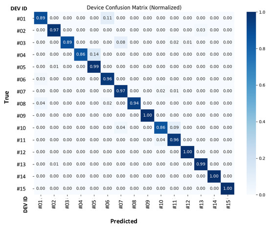
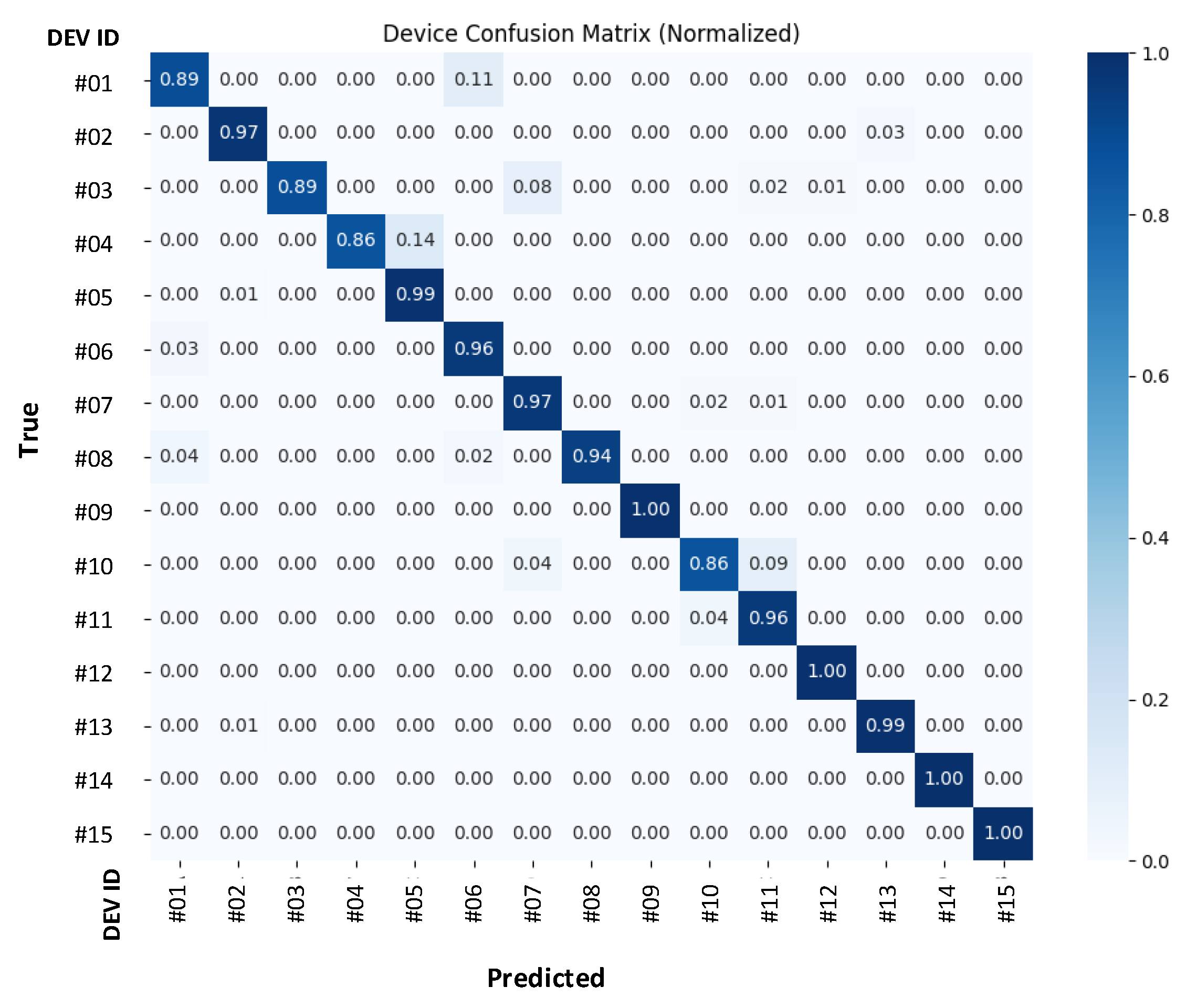
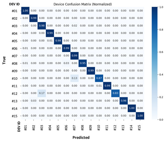
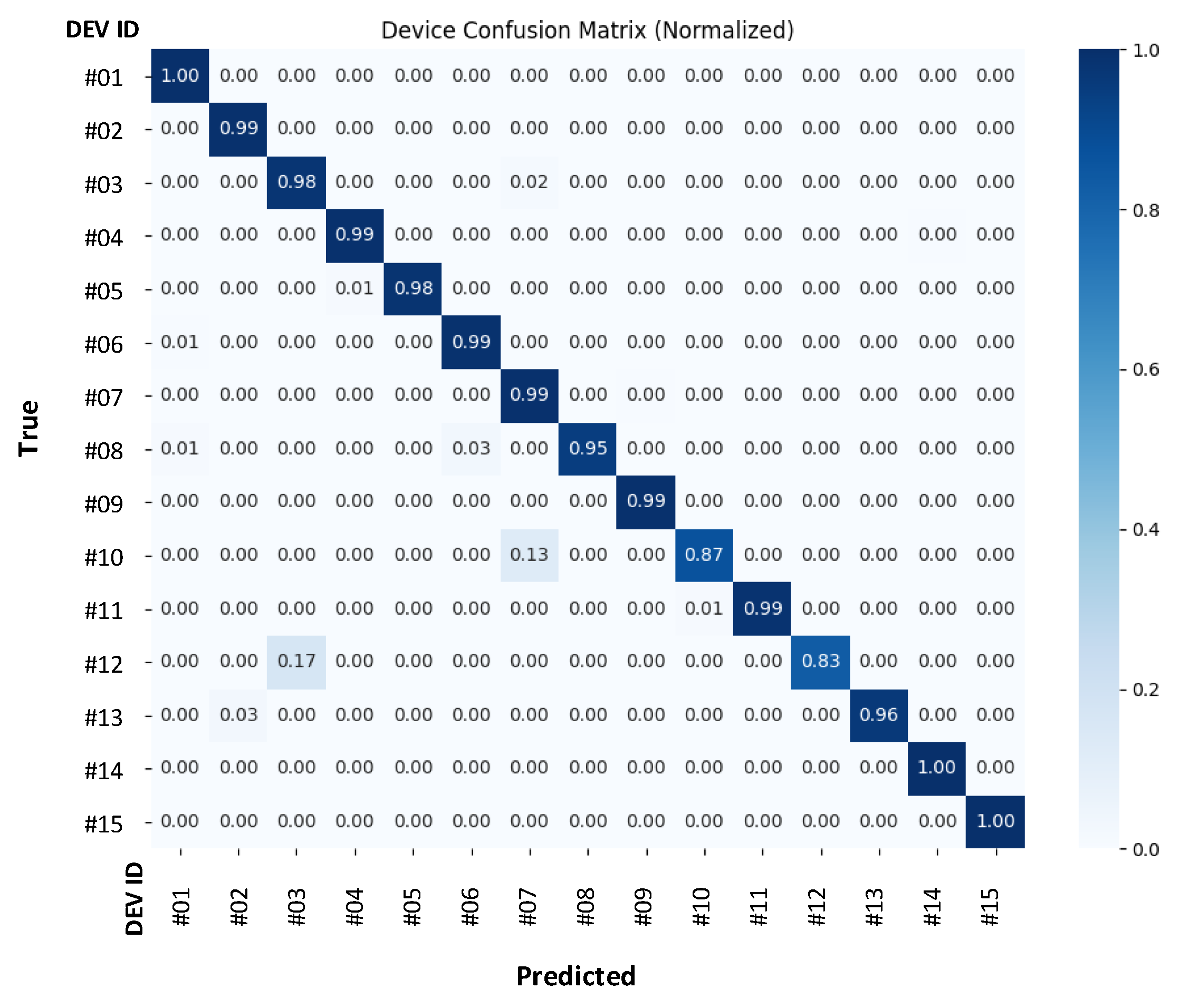
The confusion matrices for the highest accuracy values obtained in the same-scenario evaluations are presented in Figure 15 and Figure 16. Considering the type and number of TX devices used in the experiments, the confusion matrices indicate promising device classification performance on unseen data.

Figure 15. Confusion matrix obtained with training in SL (Ch E augmented with 20 channels)—test in Ch B of SL scenario.

Figure 16. Confusion matrix obtained with training in ML (Ch K augmented with 20 channels per device)—test in Ch D of ML scenario.

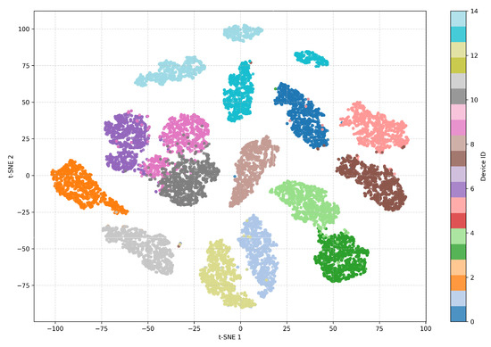
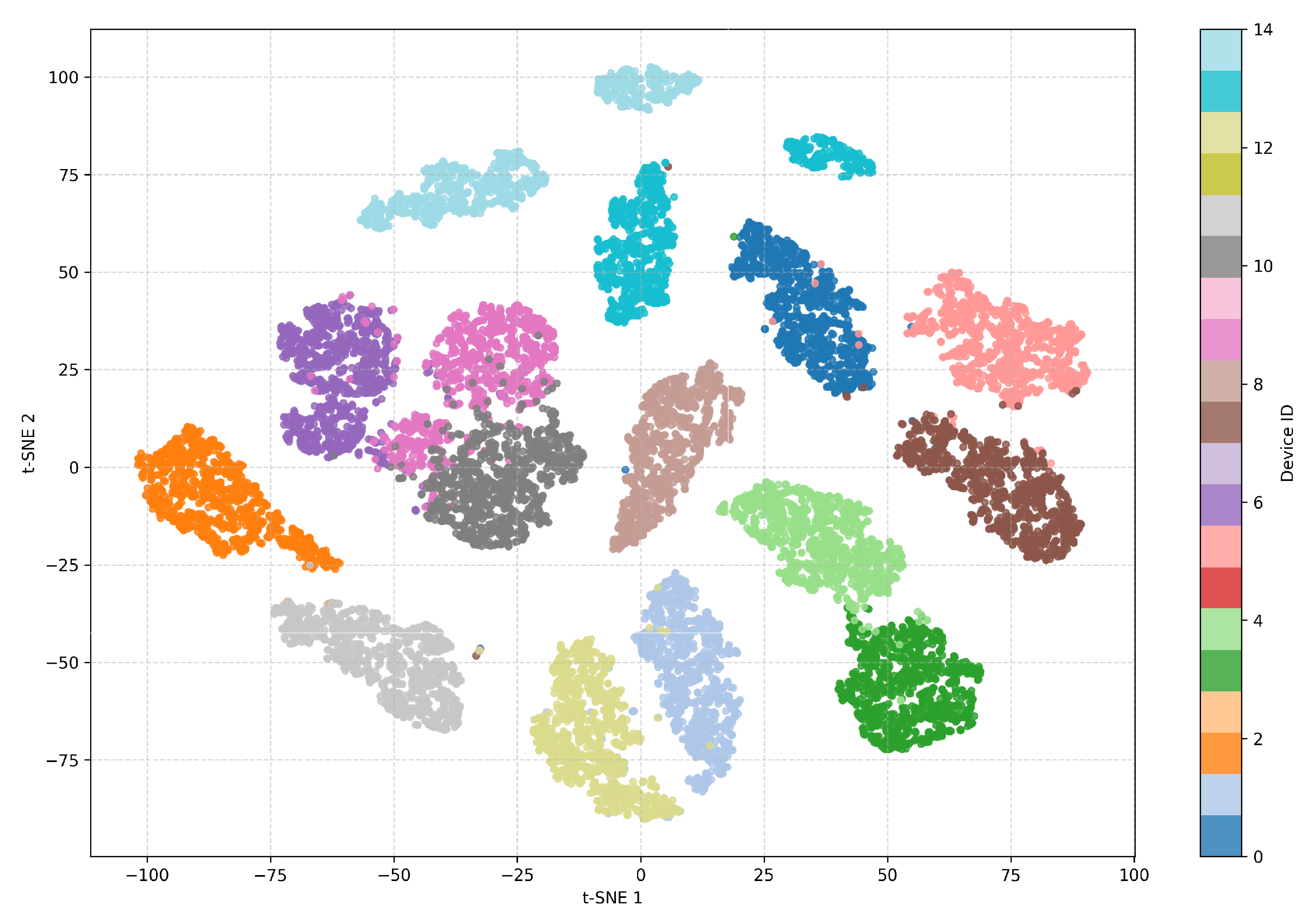
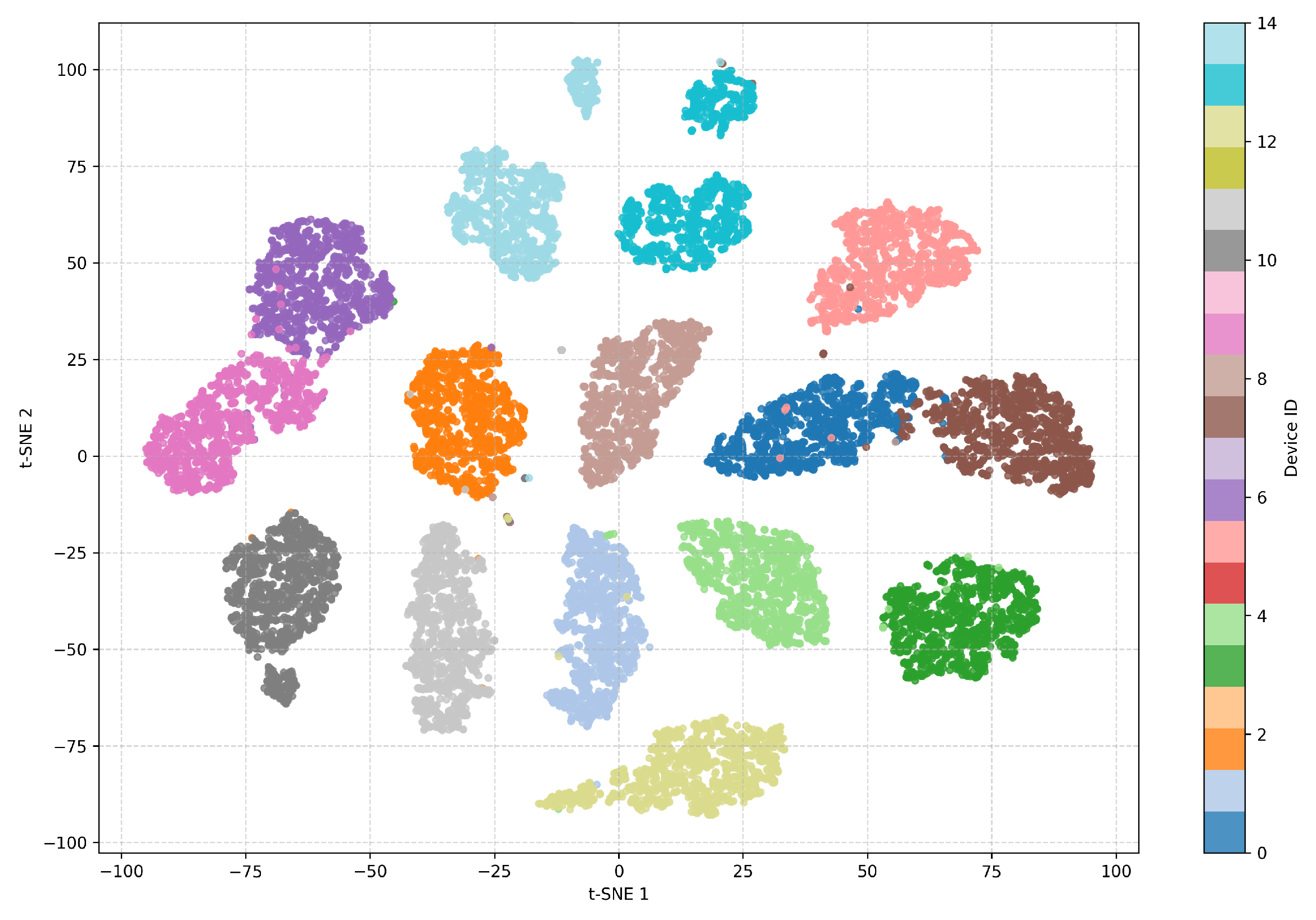
Furthermore, to visually interpret the latent features, two-dimensional t-distributed stochastic neighbor embedding (t-SNE) plots were generated. Referring to Figure 15 and Figure 16, the corresponding t-SNE plots are demonstrated in Figure 17 and Figure 18, respectively. Apparently, the embeddings belonging to device-specific latent features can be distinguished.

Figure 17. t-SNE visualization for test dataset of Ch B under SL scenario.

Figure 18. t-SNE visualization for test dataset of Ch D under ML scenario.

7. Conclusions

In this paper, device identification is performed using channel-robust RF fingerprints based on raw I/Q data. The proposed TripletDANN takes advantage of the triplet and adversarial losses. To accomplish this, in addition to device labels, standard and fine-grained channel labels are used to improve the test accuracy under unseen channel conditions. In this work, channel labels are determined based on receiver/transmitter locations and do not cover time/frequency diversity or fast fading. Legacy 802.11n signals from 15 Wi-Fi transmitters are used as case studies. Two different data collection scenarios, a single location of TXs and multiple locations of TXs, are investigated within the same- and cross-evaluation cases. Data aggregation is utilized to obtain more data from different channels to enable the use of triplet datasets and domain adversarial loss. For the same evaluation cases of both data collection scenarios, the proposed TripletDANN achieves average device classification accuracies of about 85–88% across all unseen channels. TripletDANN outperforms its counterpart model by up to $5\%$ in cross-evaluation cases. Data augmentation is also used to enhance datasets derived from different channels, resulting in mean classification accuracies of 91.82–93.30% in the same-scenario evaluation and 84.16–89.79% in the cross-scenario evaluation. Another aspect to mention is that if data augmentation or aggregation is not eligible, then it is recommended to train the network using data collected with transmitters placed at a single location.

In future work, the performance of TripletDANN will be evaluated in experiments that include dynamic channels and non-line-of-sight scenarios. In addition, triplet sampling strategies, as well as alternative contrastive learning paradigms, will be systematically investigated.

References

- Danev, B.; Zanetti, D.; Čapkun, S. On physical-layer identification of wireless devices. ACM Comput. Surv. 2012, 45, 6. [Google Scholar] [CrossRef] [Scilit]
- Üreten, O.; Serinken, N. Wireless security through RF fingerprinting. Can. J. Electr. Comput. Eng. 2007, 32, 27–33. [Google Scholar] [CrossRef] [Scilit]
- Danev, B.; Capkun, S. Transient-based identification of wireless sensor nodes. In Proceedings of the International Conference on Information Processing in Sensor Networks (IPSN); IEEE: New York, NY, USA, 2009; pp. 25–36. [Google Scholar]
- Köse, M.; Taşcıoğlu, S.; Telatar, Z. RF fingerprinting of IoT devices based on transient energy spectrum. IEEE Access 2019, 7, 18715–18726. [Google Scholar] [CrossRef] [Scilit]
- Stankowicz, J.; Robinson, J.; Carmack, J.M.; Kuzdeba, S. Complex neural networks for radio frequency fingerprinting. In Proceedings of the IEEE Western New York Image and Signal Processing Workshop (WNYISPW); IEEE: New York, NY, USA, 2019; pp. 1–5. [Google Scholar]
- Al-Shawabka, A.; Restuccia, F.; D’oro, S.; Jian, T.; Rendon, B.C.; Soltani, N.Y.; Dy, J.G.; Chowdhury, K.R.; Ioannidis, S.; Melodia, T. Exposing the fingerprint: Dissecting the impact of the wireless channel on radio fingerprinting. In Proceedings of the IEEE Conference on Computer Communications (INFOCOM); IEEE: New York, NY, USA, 2020; pp. 646–655. [Google Scholar]
- Restuccia, F.; D’Oro, S.; Melodia, T.; Chowdhury, K.R. DeepRadioID: Real-time channel-resilient optimization of deep learning–based radio fingerprinting algorithms. In Proceedings of the IEEE Conference on Computer Communications (INFOCOM); IEEE: New York, NY, USA, 2019; pp. 121–129. [Google Scholar]
- Sankhe, K.; Belgiovine, M.; Zhou, F.; Riyaz, S.; Ioannidis, S.; Chowdhury, K.R. ORACLE: Optimized radio classification through convolutional neural networks. In Proceedings of the IEEE International Conference on Computer Communications (INFOCOM); IEEE: New York, NY, USA, 2019; pp. 370–378. [Google Scholar] [CrossRef] [Scilit]
- Xing, Y.; Hu, A.; Zhang, J.; Peng, L.; Wang, X. Design of a channel-robust radio frequency fingerprint identification scheme. IEEE Internet Things J. 2023, 10, 6946–6959. [Google Scholar] [CrossRef] [Scilit]
- Shen, G.; Zhang, J.; Marshall, A.; Cavallaro, J.R. Towards scalable and channel-robust radio frequency fingerprint identification for LoRa. IEEE Trans. Inf. Forensics Secur. 2022, 17, 774–787. [Google Scholar] [CrossRef] [Scilit]
- Chen, T.; Hu, A.; Zhang, S. Fighting fire with fire: Channel-independent RF fingerprinting via the ratio of linear to logarithmic differential spectrum. IEEE Wirel. Commun. Lett. 2025, 14, 1999–2003. [Google Scholar] [CrossRef] [Scilit]
- Wang, J.; Zhang, B.; Zhang, J.; Yang, N.; Wei, G.; Guo, D. Specific emitter identification based on deep adversarial domain adaptation. In Proceedings of the 4th International Conference on Information Communication and Signal Processing (ICICSP); IEEE: New York, NY, USA, 2021; pp. 104–109. [Google Scholar] [CrossRef] [Scilit]
- Liu, J.; Wang, J.; Huang, H.; Li, J. Specific emitter identification unaffected by time through adversarial domain adaptation and continual learning. Eng. Appl. Artif. Intell. 2024, 138, 109324. [Google Scholar] [CrossRef] [Scilit]
- He, J.; Xie, Y.; Liu, X. Channel-robust specific emitter identification based on domain-adversarial training of neural networks and multi-feature fusion. IEEE Access 2025, 13, 153093–153104. [Google Scholar] [CrossRef] [Scilit]
- Reus-Muns, G.; Jaisinghani, D.; Sankhe, K.; Chowdhury, K.R. Trust in 5G open RANs through machine learning: RF fingerprinting on the POWDER PAWR platform. In Proceedings of the IEEE Global Communications Conference (GLOBECOM); IEEE: New York, NY, USA, 2020; pp. 1–6. [Google Scholar] [CrossRef] [Scilit]
- Gaskin, J.; Elmaghbub, A.; Hamdaoui, B.; Wong, W.-K. Deep learning model portability for domain-agnostic device fingerprinting. IEEE Access 2023, 11, 86801–86823. [Google Scholar] [CrossRef] [Scilit]
- Ma, J.; Zhang, J.; Shen, G.; Peng, L.; Marshall, A. Towards channel-robust radio frequency fingerprint identification using contrastive learning. In Proceedings of the IEEE Wireless Communications and Networking Conference (WCNC); IEEE: New York, NY, USA, 2025; pp. 1–6. [Google Scholar] [CrossRef] [Scilit]
- Soltani, N.; Sankhe, K.; Dy, J.G.; Ioannidis, S.; Chowdhury, K.R. More is better: Data augmentation for channel-resilient RF fingerprinting. IEEE Commun. Mag. 2020, 58, 66–72. [Google Scholar] [CrossRef] [Scilit]
- IEEE Std 802.11-2012; IEEE Standard for Information Technology—Telecommunications and Information Exchange Between Systems—Local and Metropolitan Area Networks—Specific Requirements—Part 11: Wireless LAN Medium Access Control (MAC) and Physical Layer (PHY) Specifications. IEEE: New York, NY, USA, 2012. [CrossRef] [Scilit]
- Richards, M.A. Principles of Modern Radar: Basic Principles; SciTech Publishing: Raleigh, NC, USA, 2010; Volume 1. [Google Scholar]
- Kay, S.M. Fundamentals of Statistical Signal Processing: Detection Theory; Prentice Hall: Englewood Cliffs, NJ, USA, 1998. [Google Scholar]
- Soltani, N.; Roy, D.; Chowdhury, K. PRONTO: Preamble overhead reduction with neural networks for coarse synchronization. IEEE Trans. Wirel. Commun. 2023, 22, 7848–7861. [Google Scholar] [CrossRef] [Scilit]
- MathWorks. WlanPacketDetect—Estimate Timing Offset of OFDM Packet Using L-STF. MATLAB & Simulink Documentation. Available online: https://www.mathworks.com/help/wlan/ref/wlanpacketdetect.html (accessed on 31 December 2025).
- Mohseni, S. Study the Carrier Frequency Offset (CFO) for Wireless OFDM. Master’s Thesis, Department of Electrical and Computer Engineering, University of Denver, Denver, CO, USA, 2013. Available online: https://digitalcommons.du.edu/etd/438 (accessed on 2 January 2026).
- MathWorks. WlanCoarseCFOEstimate—Perform Coarse Carrier Frequency offset (CFO) Estimation. MATLAB & Simulink Documentation. Available online: https://www.mathworks.com/help/wlan/ref/wlancoarsecfoestimate.html (accessed on 4 January 2026).
- MathWorks. WlanSymbolTimingEstimate—Estimate Symbol Timing Offset of OFDM Packet Using L-STF. MATLAB & Simulink Documentation. Available online: https://www.mathworks.com/help/wlan/ref/wlansymboltimingestimate.html (accessed on 2 January 2026).
- MathWorks. WlanFineCFOEstimate—Estimate Fractional Carrier Frequency Offset of OFDM Packet. MATLAB & Simulink Documentation. Available online: https://www.mathworks.com/help/wlan/ref/wlanfinecfoestimate.html (accessed on 2 January 2026).
- Hanna, S.; Karunaratne, S.; Cabric, D. WiSig: A large-scale WiFi signal dataset for receiver- and channel-agnostic RF fingerprinting. IEEE Access 2022, 10, 22808–22818. [Google Scholar] [CrossRef] [Scilit]
- Taşcıoğlu, S.; Köse, M.; Soysal, G. Sequential transient detection for RF fingerprinting. Electronics 2022, 11, 3333. [Google Scholar] [CrossRef] [Scilit]
- Arjovsky, M.; Shah, A.; Bengio, Y. Unitary evolution recurrent neural networks. In Proceedings of the 33rd International Conference on Machine Learning (ICML); ACM: New York, NY, USA, 2016; pp. 1120–1128. [Google Scholar]
- Guberman, N. On complex valued convolutional neural networks. arXiv 2016, arXiv:1602.09046. [Google Scholar] [CrossRef] [Scilit]
- Yang, J.; Gu, H.; Hu, C. Deep complex-valued convolutional neural network for RF fingerprinting. Drones 2022, 6, 374. [Google Scholar] [CrossRef] [Scilit]
- Huang, K.; Yang, J.; Liu, H.; Hu, P. Deep adversarial neural network for specific emitter identification under varying frequency. Bull. Pol. Acad. Sci. Tech. Sci. 2021, 69, 136737. [Google Scholar] [CrossRef] [Scilit]
- Zeng, D. Comparing contrastive and triplet loss: Variance analysis and optimization behavior. arXiv 2025, arXiv:2510.02161v2. [Google Scholar] [CrossRef] [Scilit]
- Ganin, Y.; Ustinova, E.; Ajakan, H.; Germain, P.; Larochelle, H.; Laviolette, F.; Marchand, M.; Lempitsky, V. Domain-adversarial training of neural networks. J. Mach. Learn. Res. 2016, 17, 35. [Google Scholar]
- Erceg, V.; Schumacher, L.; Kyritsi, P.; Baum, D.S.; Gorokhov, A.Y.; Oestges, C.; Li, Q.; Yu, K.; Tal, N.; Dijkstra, B.; et al. TGn Channel Models. IEEE 802.11-03/940r4, Version 4. 2004. Available online: https://www.google.com/url?sa=t&source=web&rct=j&opi=89978449&url=https://mentor.ieee.org/802.11/dcn/03/11-03-0940-04-000n-tgn-channel-models.doc&ved=2ahUKEwiUoeOosIOTAxXkOjQIHXeYOp0QFnoECBgQAQ&usg=AOvVaw09gOnPU8C2MU8wNHtZs-Wc (accessed on 4 January 2026).
- MathWorks. WlanTGnChannel System Object—TGn Multipath Fading Channel for IEEE 802.11n. MATLAB & Simulink Documentation. Available online: https://www.mathworks.com/help/wlan/ref/wlantgnchannel-system-object.html (accessed on 4 January 2026).
- Miuccio, L.; Panno, D.; Riolo, S. A flexible encoding/decoding procedure for 6G SCMA wireless networks via adversarial machine learning techniques. IEEE Trans. Veh. Technol. 2023, 72, 3288–3303. [Google Scholar] [CrossRef] [Scilit]
- Ma, J.; Zhang, J.; Shen, G.; Peng, L.; Marshall, A. Toward channel-robust and receiver-independent radio frequency fingerprint identification. IEEE Trans. Inf. Forensics Secur. 2025, 20, 12112–12125. [Google Scholar] [CrossRef] [Scilit]
Disclaimer/Publisher’s Note: The statements, opinions and data contained in all publications are solely those of the individual author(s) and contributor(s) and not of MDPI and/or the editor(s). MDPI and/or the editor(s) disclaim responsibility for any injury to people or property resulting from any ideas, methods, instructions or products referred to in the content. |
© 2026 by the authors. Licensee MDPI, Basel, Switzerland. This article is an open access article distributed under the terms and conditions of the Creative Commons Attribution (CC BY) license.