Lightweight Network Design for Joint Detection and Modulation Recognition of LPI Radar Signals with Knowledge Distillation

Abstract

In the field of electronic support and radar warning, it is necessary to effectively detect and recognize the modulation types of non-cooperative radar signals, especially for radars with Low Probability of Intercept (LPI) waveforms. Multiple intelligent detection and recognition algorithms based on the Transformer architecture have been proposed, achieving good performance even under low signal-to-noise ratio (SNR). However, Transformer-based radar intelligent detection and recognition algorithms have a huge number of parameters coupled with complex structures, which will result in significant power consumption and computational latency when deployed on general computing platforms. To address the above issues, this paper proposes a lightweight design for Transformer-based radar signal intelligent detection and recognition networks. A Lightweight Joint Detection and Modulation Recognition Networks (JDMR-LNet) is designed. To enhance the feature extraction ability of lightweight networks, this paper designed a hybrid model distillation method. The experimental results demonstrate that, compared with the directly trained JDMR-LNet, the accuracy of automatic modulation type recognition of the JDMR-LNet after distillation is increased by 2.37% at −12 dB, and the signal detection is increased by 2.07% at −10 dB. The number of parameters of the JDMR-LNet has also decreased significantly. Compared with the original model, the JDMR-LNet is compressed by 11.18 times. Furthermore, this paper completed FPGA deployment of the JDMR-LNet model, with simulation verifying its functional correctness.

1. Introduction

Electronic support is a part of electronic warfare, referring to a series of actions involving the search, interception, identification, and localization of electromagnetic radiation sources [1]. One of the representative issues in electronic support is the signal detection (SD) and automatic modulation recognition (AMR) of Low Probability of Intercept (LPI) radar signals [2], which have characteristics such as low peak power, large time-bandwidth product, frequency agility, and compound modulations [3]. Signal detection in radar refers to the task of processing the received radar echo signal to assess the presence of radar pulses [4]. Automatic modulation recognition involves analyzing and processing signals to identify the modulation scheme used and classify them. In radar systems, signal detection is crucial as it directly impacts the performance and accuracy of the radar system and automatic modulation recognition also directly affects the correctness of the output results of the radar system [5]. Traditional detection and recognition methods generally exhibit higher identification accuracy when the signal-to-noise ratio (SNR) is above 0 dB, but with a sharp decrease in accuracy as the SNR decreases, indicating poor robustness.

In recent years, with the development of deep learning, SD and AMR methods based on deep learning have attracted wide attention due to their efficient learning ability and better detection performance [6,7,8]. More and more researchers are applying them to radar signal detection and automatic modulation recognition.

Most of the existing deep learning-based signal detection and automatic modulation classification consider signal detection and automatic modulation classification as two cascaded tasks: First, a pulse is detected in the SD task, and then the pulse is sent to the AMR task for processing [9]. However, since the energy of the signal is distributed in both the time-frequency domain and the energy distribution patterns are modulation-specific, applying this modulation-type information to the SD task can yield better results and simplify the traditional processing chain. To this end, Joint Detection and Modulation Recognition Networks (JDMR-Net) is a multi-task learning framework based on Transformer, that efficiently performs radar signal detection and automatic modulation classification tasks simultaneously [10].

However, deep neural networks have a huge number of parameters, making it difficult to deploy them on embedded devices with strict limitations on memory, computing resources, and power consumption [11,12]. Therefore, one of the current research focuses is how to design lightweight networks with simpler structures and fewer parameters [13]. Model compression methods for deep neural networks include pruning, low-rank decomposition, compact network design, quantization, and knowledge distillation. Parameter pruning-based methods exploit the redundancy inherent in model parameters, aiming to reduce the total number of model parameters by eliminating redundant and non-critical components [14]. Low-rank decomposition utilizes tensor decomposition of matrices to compress the information of deep neural network weight parameters [15]. Compact network design reduces the parameter space by designing special network structures, thereby saving storage and computational resources [16,17]. The method based on quantization represents the floating-point weights or activation output values in the network with low-bit fixed-point numbers to reduce the storage space occupied by the network [18].

Knowledge distillation trains a more compact neural network to reproduce the inference effects of a larger model [19,20]. This method involves constructing a lightweight model (commonly referred to as the student model), which is trained using supervisory signals from a larger, higher-performance model (referred to as the teacher model). In this training process, such supervisory signals are incorporated into the loss function to enhance the performance of the lightweight model [21]. The supervisory signals generated by the teacher model are defined as “knowledge” in this context, while the process by which the student model acquires such knowledge—transmitted via the teacher’s supervisory signals—is referred to as “distillation”. Knowledge distillation was first proposed by Hinton in 2015 and applied to classification tasks [22]. Subsequently, Romero et al. introduced FitNets [23], which extended output layer distillation to feature distillation. In 2017, intermediate layer attention distillation (AT) was proposed [24], which is no longer limited to the representation of a specific node in the network. Feature translation and distillation were achieved through the addition of modules in 2018 with the introduction of FT. Following this, more research on the relationships between features emerged, such as RKD [25] and IRG [26]; ReviewKD proposed by Chen P et al., improves the effectiveness of knowledge distillation by leveraging the multi-layer features of the teacher model to guide the single-layer feature learning of the student model [27]. TinyMIM designs a distillation scheme for Transformer models, utilizing the relationships between the Q, K, and V matrices of corresponding layers in the teacher and student models for distillation [28]. For distillation of heterogeneous models, Hao Z et al. introduced a branching structure in the intermediate layers of the student model, which projects the intermediate layer features into the logits space and trains the branch using the logits output from the teacher [29].

Each of these compression and acceleration methods can achieve good results when used individually, but they also have their own limitations. To meet the requirements for model lightweighting in the radar field and edge deployment, this study integrates multiple distillation methods, applies them to the radar field, and distills the lightweight network to enhance its edge deployment performance. Therefore, this paper selects the JDMR-Net as an example and designs a lightweight network. By analyzing the functions of various network structures in JDMR-Net, corresponding lightweight designs and pruning are applied to simplify the network structure and reduce the number of parameters, resulting in a lightweight model called JDMR-LNet, which is used as the student model in model distillation. Subsequently, network branch structures are designed to extract regional information of pulse signals in the input sequence for feature distillation. Relationship distillation is then employed to enhance the feature extraction capability of the student model’s attention layers due to the insufficient feature extraction caused by the fewer attention layers in the student model [30]. Finally, a hybrid distillation approach combining relationship distillation and feature distillation is proposed, along with the total distillation loss expression.

The main contributions of the text can be summarized as follows:

(1) Taking JDMR-Net as an example, a lightweight structure is designed for the Transform-based network to obtain JDMR-LNet.

(2) After the lightweight model design, we employed knowledge distillation to enhance the performance of JDMR-LNet, ensuring it maintains excellent detection and recognition capabilities under a compression ratio of 11.18.

(3) A branch structure has been designed for feature distillation, which can extract the location information of pulse signals. Through feature distillation, the signal detection probability of the student model can be improved at various SNRs.

(4) By combining feature distillation with relation distillation, not only is the signal detection probability of the student model significantly improved, but also the accuracy of automatic modulation recognition is enhanced.

(5) The conversion of the JDMR-LNet for deployment on the FPGA platform has been completed, and corresponding simulation tests have been conducted.

2. Problem Formulation

To perform the SD task and AMR tasks, this paper formulates the radar signal detection and modulation recognition as a multi-task learning (MTL) problem. Subsequently, the formulation of the knowledge distillation is introduced.

2.1. Multi-Task Learning

Given m learning tasks ${\left\{T\right\}}_{i=1}^m$, where all or a subset of the tasks are related, MTL is a paradigm in which these m tasks are jointly learned via a unified network, enabling knowledge from one task to benefit others [31,32]. In this paper, we adopt a scheme that shares hidden layers across all tasks while maintaining multiple task-specific output layers.

The joint SD and AMR tasks formulated as an MTL problem can be denoted as $T=\{T_{\mathrm{SD}},T_{\mathrm{AMR}}\}$, where $T_{\mathrm{SD}}$ and $T_{\mathrm{AMR}}$ represent the SD and AMR tasks, respectively. Let $X=\left\{x_i\right|1\le i\le N\}$ denote the training data, and the corresponding training targets are given by $\mathrm{Y}=\left\{(y_i^{\mathrm{SD}},y_i^{\mathrm{AMR}})\right|1\le i\le N\}$, where N is the number of samples. These two tasks share the same training data, while their corresponding $\mathrm{Y}$ varies across tasks. For the i-th signal sample containing M pulses, the SD task provides the starting position $b_j^{\mathrm{s}}$ and ending position $b_j^{\mathrm{e}}$ of the j-th pulse, denoted as $y_i^{\mathrm{D}}=\left\{(b_j^{\mathrm{s}},b_j^{\mathrm{e}})\right|1\le j\le M\}$. The corresponding modulation types of the detected pulses are obtained through the AMR task, denoted as $y_i^{\mathrm{R}}=\left\{c_j\right|1\le j\le M\}$. Therefore, the function $F^{\mathrm{MTL}}:X\to \mathrm{Y}$ is constructed using the training dataset, mapping the data space X to the corresponding target space $\mathrm{Y}$. For a test signal sample, the learned function $F^{\mathrm{MTL}}$ concurrently solves the SD and AMR tasks to generate outputs for each task.

2.2. Model Lightweight

In model lightweight, the problem function aims to train a lightweight student model $f_s$ to mimic the knowledge of a pre-trained large teacher model $f_t$, such that $f_s$ achieves comparable performance to $f_t$ with lower computational cost. Formally, given a dataset $\mathcal{D}={\left\{(x_i,y_i)\right\}}_{i=1}^N$ where $x_i$ is the input sample and $y_i\in \{1,2,\dots ,C\}$ is the true label (with C being the number of classes), the student model is optimized by minimizing a weighted combination of two loss terms: Hard loss measures the discrepancy between the student’s predictions and the true labels. Soft loss captures the “dark knowledge” from the teacher’s softened predictions. The student model is trained by minimizing the joint loss function to leverage both the true labels and the teacher’s implicit knowledge.

3. Method

In this section, an overall procedure of the method is first provided, followed by a detailed account of the teacher model, the student model, and the design of the two distillation methods, and finally, the overall loss function is presented.

3.1. Overall Procedure

Based on the referenced original network model, we first designed a teacher model with a structure more suitable for the knowledge distillation process. Then, a lightweight student model (JDMR-LNet) was designed based on the teacher model. For the dual tasks, two distillation methods—feature distillation and attention distillation—were designed, and they were combined to enhance the performance of the student model.

3.2. Teacher Model

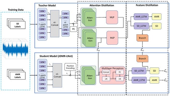
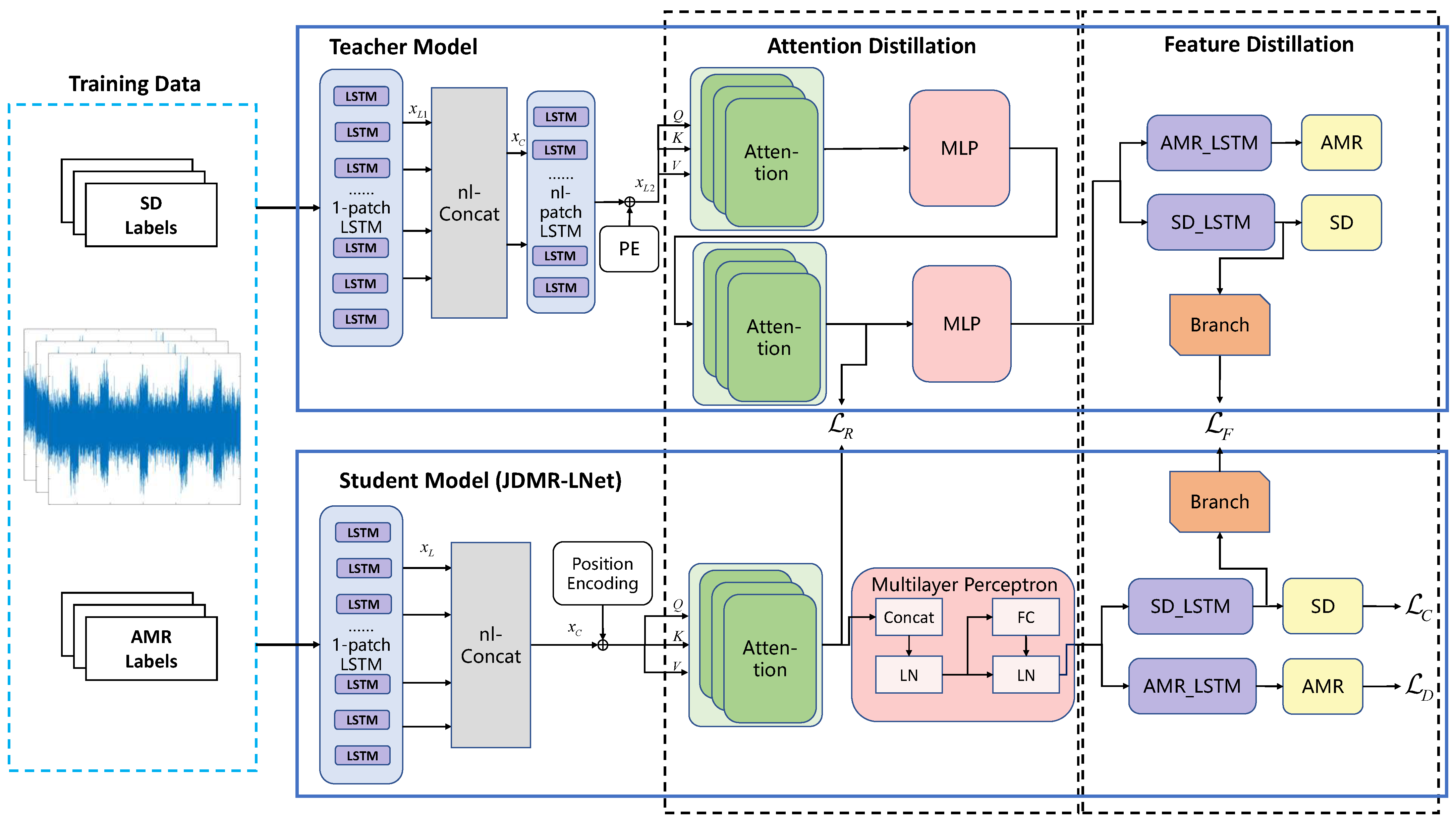
In JDMR-Net, a cross-attention mechanism is employed to process the information preprocessed by previous stages. Although the cross-attention mechanism excels in feature extraction, its intricate structure introduces model heterogeneity when used as the architecture for the subsequent teacher model. This heterogeneity makes it challenging for the student model to effectively acquire knowledge via distillation. Therefore, we first designed a simplified teacher model. Compared to the original JDMR-Net, this simplified version replaces the cross-attention layer with a self-attention layer while keeping all other components unchanged. The resultant simplified JDMR-Net serves as the teacher model for subsequent distillation operations. The structure of the teacher model is illustrated in Figure 1.

Figure 1. The above figure shows the structures of the teacher model and student model, as well as the distillation design. In the figure, PE is the abbreviation of the Position Encoding module, MLP is the abbreviation of the Multilayer Perceptron module, and the nl-concate module concatenates every nl adjacent feature vector from the single-scale LSTM output into a new patch.

3.3. Student Model (JDMR-LNet)

This section first analyzes the functions of key network structures within the teacher model, laying a foundation for subsequent lightweight optimization. On this basis, structure-specific lightweight design and parameter pruning are carried out for each key structure, with the core goal of reducing model redundancy while preserving the network’s core detection and recognition performance. Through this series of targeted optimization processes, a lightweight intelligent detection and recognition network for radar signals is developed, which is formally designated as JDMR-LNet. As the direct product of functional analysis and structural optimization based on the teacher model, this JDMR-LNet will serve as the student model in the subsequent model distillation process to further enhance its comprehensive performance.

Data Preprocessing: The first step for the teacher model is data preprocessing. In order to effectively extract features from the input sequence, enhance the parallel processing capability of subsequent processing steps, and address the potential vanishing gradient problem during the model training of LSTM with long input sequences, the input signal is divided into multiple smaller patches.

Let the radar signal sampling sequence to be processed be denoted as $\mathbf{X}\in {\mathbf{R}}^{T\times 2}$, which is a matrix of size T, where T is the length of the sequence to be processed, and each data point in the sequence contains two values: the real part and the imaginary part. In the preprocessing step, the signal is divided into n patches, each of length w, denoted as ${\mathbf{X}}^i(1\le i\le n)$. Therefore, the entire sequence to be processed can be represented as shown in Equation (1):

$$\mathbf{X}=\left[{\mathbf{X}}^1,{\mathbf{X}}^2,\dots ,{\mathbf{X}}^n\right],{\mathbf{X}}^i\in {\mathbf{R}}^{w\times 2}$$

(1)

The relationship between the sequence length T, the number of patches n, the patch length w, and the sliding step p is

$$T=(\mathrm{n}-1)\times p+w$$

(2)

From the ablation experiments, it is evident that data preprocessing has a crucial impact on the final results; therefore, JDMR-LNet still employs this preprocessing as its first component.

Local Feature Extraction: In the teacher model, after preprocessing, the sequence to be processed is divided into n patches of length w: ${\mathbf{X}}^i(1\le i\le n)$. These patches will be used to extract features at different time scales through a dual-scale LSTM. The “1-patch scale LSTM” is used to learn the time-series relationships within the sequence patches, and its output consists of n feature vectors with a dimension of $u1$, denoted as ${\mathbf{X}}_{L1}^i(1\le i\le n)$. Next, concatenate every $n_l$ adjacent feature vectors in $X_{L1}$ to form $n/n_l$ matrices, denoted as ${\mathbf{X}}_C^i(1\le i\le n/n_l)$. Then, $X_C$ is used as input data for the “nl-patch scale” LSTM, which extracts temporal features at the scale of $n_l$ patches. The output of the “nl-patch scale” LSTM is denoted as ${\mathbf{X}}_{L2}^i(1\le i\le n/n_l)$.

Corresponding to the local feature extraction part of the teacher model, JDMR-LNet is a single-layer LSTM. Unlike the dual-scale LSTM, in JDMR-LNet a single-layer LSTM is used to extract signal features within the patch, while the extraction of features between patches is handled by subsequent network layers.

Global Similarity Mining: After local feature extraction, we obtain $X_C$ and $X_{L2}$, which contain hierarchical features from a single patch and adjacent $n_1$ patches, respectively. In the global feature extraction part, the teacher model extracts the global similarity of feature vectors $X_C$ and $X_{L2}$ through a two-layer cross-attention structure. Before inputting $X_C$ and $X_{L2}$ into the Cross Attention layer, the teacher model adds positional encoding to retain the relative positional information of the sequence. Encoder 1 selects $X_C$ as the input for the query and $X_{L2}$ as the input for the key and value. Encoder 2 selects $X_{L2}$ as the input for the query and $X_C$ as the input for the key and value. Here, the encoder is exactly the same as the encoder in the Transformer, which includes sub-layers such as multi-head attention, feed-forward neural networks, residual connections, and layer normalization. The output of the first layer of self-attention serves as the input for the second layer of self-attention.

Therefore, the third part of JDMR-LNet is a single-layer encoder, which corresponds to the self-attention layer in the teacher model. In the teacher model, the two output results from the dual-scale LSTM are used as part of the input for the two encoders in the self-attention layer, allowing the self-attention layer to learn the features between patches. The attention mechanism in Transformers has a high computational complexity, and the cross-attention mechanism in JDMR-Net further increases the model’s complexity. To simplify the computation, JDMR-LNet employs only a single-layer encoder to extract features between patches through self-attention.

Task Head: The fourth part of JDMR-LNet is the task head output layer, which corresponds to the task head in the teacher model, responsible for completing the tasks of signal detection and modulation type recognition. The task head in JDMR-LNet consists of tensor transformations and fully connected layers, which map the results of global feature extraction into the output format required for signal detection and automatic modulation type recognition. Since the output of SD indicates the start and end positions of pulses, while the output of AMR indicates the modulation type of the signal, the task heads serve to map the input feature ${\mathbf{Z}}_S$ into the output formats required for SD and AMR. The computational expression for the task head can be represented by the following equation:

$$\begin{array}{c}{\mathbf{Y}}^{\mathrm{SD}}=\mathrm{Sigmoid}\left(\mathrm{Trans}\left({\mathbf{Z}}_S\right){\mathbf{W}}_D+{\mathrm{b}}_{\mathrm{D}}\right)\hfill \\ {\mathbf{Y}}^{\mathrm{AMR}}=\mathrm{Softmax}\left(\mathrm{Trans}\left({\mathbf{Z}}_S\right){\mathbf{W}}_R+{\mathrm{b}}_{\mathrm{R}}\right)\hfill \end{array}$$

(3)

where $W_D$, $W_R$, ${\mathrm{b}}_{\mathrm{D}}$, and ${\mathrm{b}}_{\mathrm{R}}$ represent the weights and biases of the fully connected layers in the signal detection task and automatic modulation recognition task, respectively, while $\mathrm{Trans}(\ast )$ denotes the shape transformation applied to the input tensor.

The LSTM layer between the encoder and the fully connected layer is also retained. The LSTM in the signal detection task head is used to summarize the features related to the signal detection task from the input, while the LSTM in the automatic modulation recognition task head is used to summarize the features related to the automatic modulation recognition task from the input.

The final structure of the network is shown in Figure 1. The lightweight network JDMR-LNet significantly simplifies the computational structure and reduces the number of layers in the teacher model, making it more suitable for deployment on embedded devices.

3.4. Feature Distillation

The feature map-based distillation method involves mapping the output feature maps of the target layers of the teacher model and the student model into matrices of the same size. The similarity between these two matrices is used as the distillation loss to perform distillation on the model. From Equation (2), it can be seen that when the patch size is equal to w and the sliding step p is also equal to w, the data preprocessing divides the input sequence into n patches of size w.

In the signal detection task, the start and end positions of the pulse signal must be located in one of the n regions. Therefore, a network branch composed of fully connected layers can be added to the task heads of both the teacher model and the student model.

The branch consists of a start branch and an end branch, which are used to predict the regions of the starting and ending positions of the signal, respectively. The branch structure essentially performs a multi-class classification task, and its computational expression is as follows:

$$\begin{array}{c}\mathbf{S}=\mathrm{Softmax}(\mathbf{X}{\mathbf{W}}_{\mathrm{start}}+{\mathbf{b}}_{\mathrm{start}})\hfill \\ \mathbf{E}=\mathrm{Softmax}(\mathbf{X}{\mathbf{W}}_{\mathrm{end}}+{\mathbf{b}}_{\mathrm{end}})\hfill \end{array}$$

(4)

In this context, $\mathbf{X}$ is the input to the branching structure; ${\mathbf{W}}_{\mathrm{start}}$ and ${\mathbf{b}}_{\mathrm{start}}$ are the weights and biases of the fully connected layer for the start branch; ${\mathbf{W}}_{\mathrm{end}}$ and ${\mathbf{b}}_{\mathrm{end}}$ are the weights and biases of the fully connected layer for the end branch. $\mathbf{S}\in {\mathbf{R}}^{M\times n}$ and $\mathbf{E}\in {\mathbf{R}}^{M\times n}$ are matrices of size $(M,n)$, where M is the maximum number of pulses in a single signal sequence, and n is the number of patches into which the input signal sequence is divided. The meaning of the element at position $[i,j]$ in matrix $\mathbf{S}$ is the probability that the starting position of the i-th pulse in the input sequence falls within the j-th patch; the meaning of the element at position $[i,j]$ in matrix $\mathbf{E}$ is the probability that the ending position of the i-th pulse in the input sequence falls within the j-th patch.

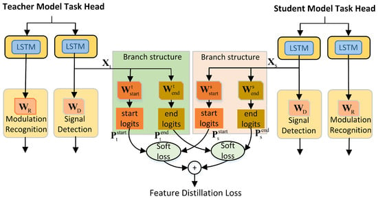
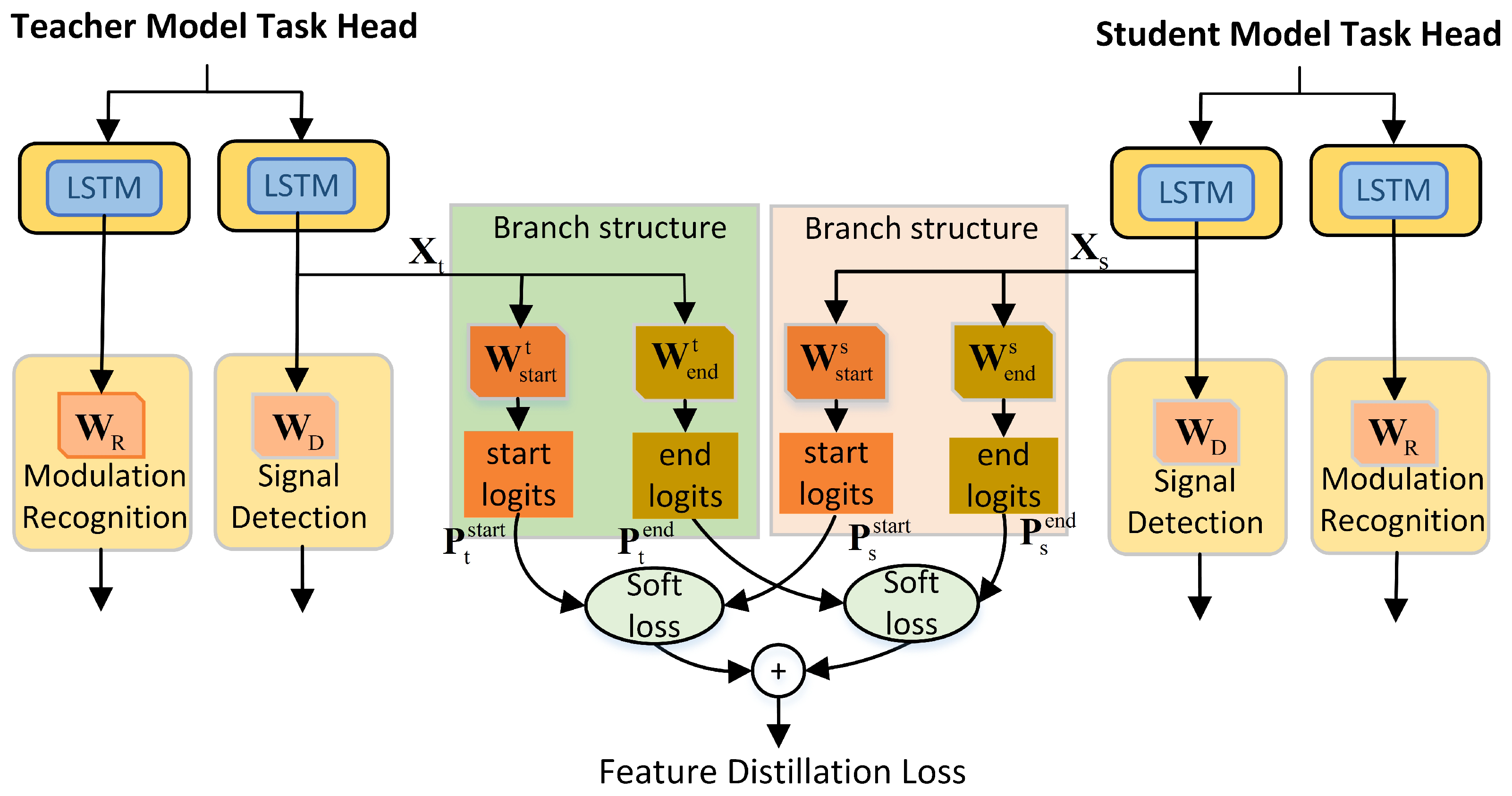
Before training the teacher model, a branch structure is added. After the training is completed, this branch structure can accurately predict the regions where the pulse starting and ending positions are located. During the distillation process, the student model learns the knowledge of the pulse regions through the branch structure, thereby enhancing its signal detection performance. The feature distillation structure is shown in Figure 2.

Figure 2. Feature distillation structure. By incorporating branch structures to convey the signal location information of the teacher model to JDMR-LNet.

The soft label loss between the teacher branch structure and the student branch structure logits in this paper is defined as the feature distillation loss, with the calculation formula given in Equation (5).

$${\mathcal{L}}_F={\mathcal{L}}_{\mathrm{soft}}({\mathbf{P}}_t^{\mathrm{start}},{\mathbf{P}}_s^{\mathrm{start}})+{\mathcal{L}}_{\mathrm{soft}}({\mathbf{P}}_t^{\mathrm{end}},{\mathbf{P}}_s^{\mathrm{end}})$$

(5)

where ${\mathcal{L}}_F$ represents the feature distillation loss. ${\mathbf{P}}_t^{\mathrm{start}}$ and ${\mathbf{P}}_s^{\mathrm{start}}$ are the probability distributions belonging to various regions output by the start branch structures of the teacher model and the student model, respectively, when the temperature coefficient is T. ${\mathbf{P}}_t^{\mathrm{end}}$ and ${\mathbf{P}}_s^{\mathrm{end}}$ are the probability distributions belonging to various regions output by the end branch structures of the teacher model and the student model, respectively, when the temperature coefficient is T. The expressions for the probability distributions and the soft label loss ${\mathcal{L}}_{\mathrm{soft}}$ are shown below.

$$\begin{array}{cc}\hfill & \mathrm{P}(z_j,T)=\mathrm{Sotfmax}(z_j/T)\hfill \\ \hfill & {\mathcal{L}}_{\mathrm{soft}}({\mathrm{P}}_t,{\mathrm{P}}_s)={\mathrm{D}}_{\mathrm{KL}}({\mathrm{P}}_t\left|\right|{\mathrm{P}}_s)\hfill \\ \hfill & ={\displaystyle \sum _{j=1}^N}{\mathrm{P}}_t(z_{t,j},T)log\left({\displaystyle \frac{{\mathrm{P}}_t(z_{t,j},T)}{{\mathrm{P}}_s(z_{s,j},T)}}\right)\hfill \end{array}$$

(6)

3.5. Attention Distillation

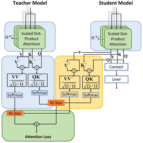
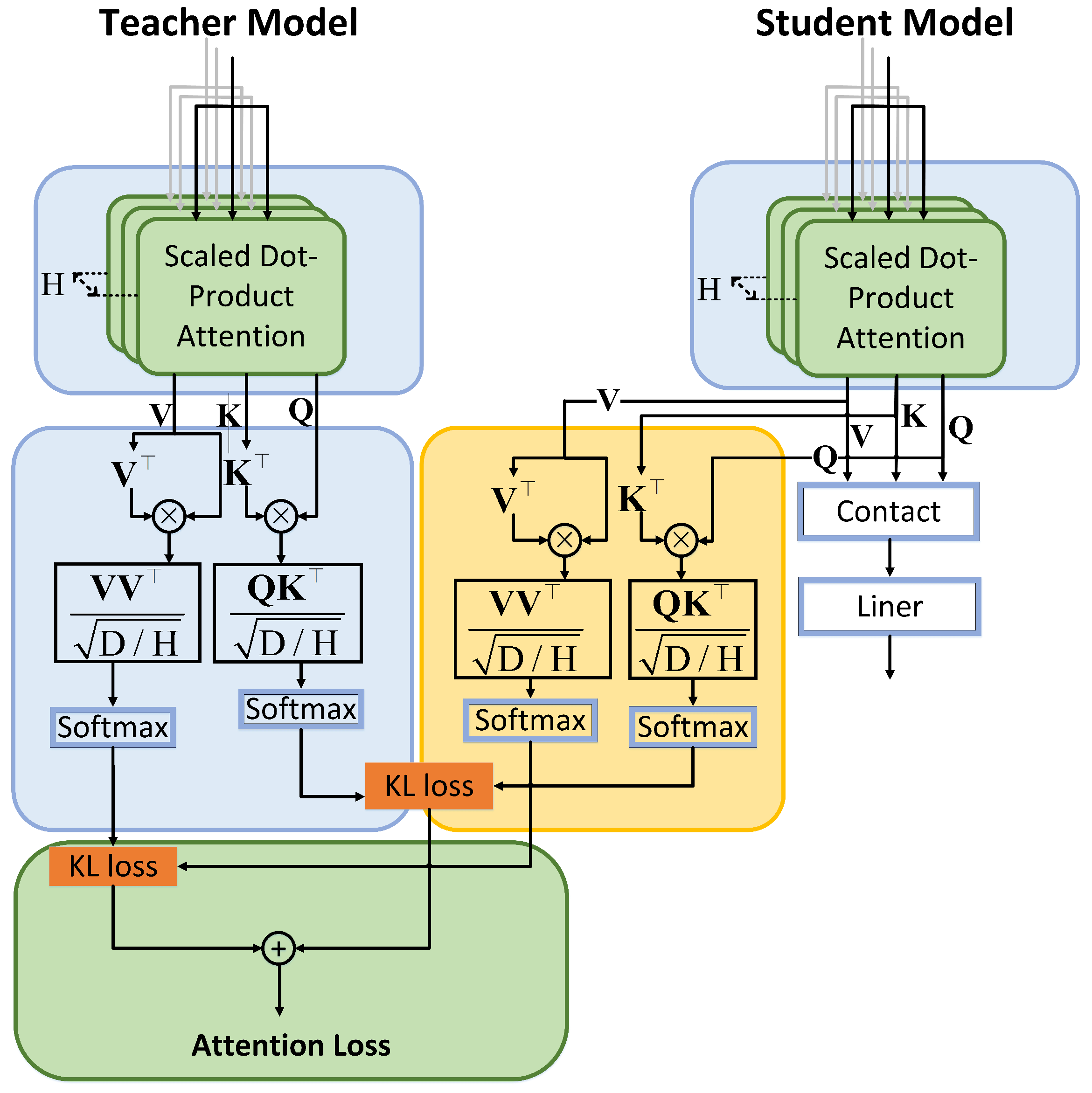
Relational distillation transforms the outputs of specific layers of the teacher model and the student model into relational matrices, using the similarity of the relational matrices from both models as the distillation loss. Multiple studies have shown that relational distillation is more effective for distilling the attention components. Therefore, in this paper, we design a distillation structure for the attention layer based on the relational distillation method as shown in Figure 3.

Figure 3. Attention distillation structure. Distillation is performed using the relationship between the QKV matrices output by the attention modules of the teacher and student models, with their KL divergence serving as the distillation loss.

Calculate the relationship matrix of the attention layer outputs V-V and Q-K as shown below.

$$\begin{array}{c}{\mathbf{R}}_{s\to h}^{QK}=\mathrm{Softmax}\left({\displaystyle \frac{{\mathbf{Q}}_s^h{\mathbf{K}}_s^{h\top }}{\sqrt{D/H}}}\right)\hfill \\ {\mathbf{R}}_{s\to h}^{VV}=\mathrm{Softmax}\left({\displaystyle \frac{{\mathbf{V}}_s^h{\mathbf{V}}_s^{h\top }}{\sqrt{D/H}}}\right)\hfill \end{array}$$

(7)

$$\begin{array}{c}{\mathbf{R}}_{t\to h}^{QK}=\mathrm{Softmax}\left({\displaystyle \frac{{\mathbf{Q}}_{t,2}^h{\mathbf{K}}_{t,2}^{h\top }}{\sqrt{D/H}}}\right)\hfill \\ {\mathbf{R}}_{t\to h}^{VV}=\mathrm{Softmax}\left({\displaystyle \frac{{\mathbf{V}}_{t,2}^h{\mathbf{V}}_{t,2}^{h\top }}{\sqrt{D/H}}}\right)\hfill \end{array}$$

(8)

where ${\mathbf{R}}_{s\to h}^{QK}$ represents the $\mathbf{Q}-\mathbf{K}$ relationship matrix predicted by the student model, while ${\mathbf{R}}_{t\to h}^{QK}$ is the target $\mathbf{Q}-\mathbf{K}$ relationship matrix output by the teacher model. Similarly, ${\mathbf{R}}_{s\to h}^{VV}$ and ${\mathbf{R}}_{t\to h}^{VV}$ are the $\mathbf{V}-\mathbf{V}$ predicted the relationship matrix of the student model and the $\mathbf{V}-\mathbf{V}$ target relationship matrix of the teacher model, respectively. D is the dimension of the input vector, H represents the total number of attention heads, and ${\mathbf{Q}}_s^h$, ${\mathbf{K}}_s^h$, and ${\mathbf{V}}_s^h$ are the outputs of $\mathbf{Q}$, $\mathbf{K}$, and $\mathbf{V}$ from the h-th attention head in the encoder of the student model; ${\mathbf{Q}}_{t,2}^h$, ${\mathbf{K}}_{t,2}^h$, and ${\mathbf{V}}_{t,2}^h$ are the outputs of $\mathbf{Q}$, $\mathbf{K}$, and $\mathbf{V}$ from the h-th attention head in the second layer encoder of the teacher model, respectively. ${(\ast )}^{\top }$ denotes the transpose of the matrix.

Finally, the KL divergence between the relationship matrices is used as the distillation loss, and the expression for the calculation is as follows:

$$\begin{array}{cc}& {\mathcal{L}}_R={\displaystyle \frac{1}{H}}{\displaystyle \sum _{h=1}^H}{\mathrm{D}}_{\mathrm{KL}}\left({\mathbf{R}}_{t\to h}^{QK}\left|\right|{\mathbf{R}}_{s\to h}^{QK}\right)+{\displaystyle \frac{1}{H}}{\displaystyle \sum _{h=1}^H}{\mathrm{D}}_{\mathrm{KL}}\left({\mathbf{R}}_{t\to h}^{VV}\left|\right|{\mathbf{R}}_{s\to h}^{VV}\right)\end{array}$$

(9)

3.6. Loss Function

The calculation of the AMR loss ${\mathcal{L}}_C$ is shown in Equation (10):

$${\mathcal{L}}_C(c,\widehat{c})={\displaystyle \frac{1}{M}}{\displaystyle \sum _{j=1}^M}\left[-c_{j}log\widehat{p}\left(c_j\right)\right]$$

(10)

where ${\mathcal{L}}_C$ represents the cross-entropy loss between the predicted values $\widehat{c}$ and the true values c, $\widehat{p}\left(c_j\right)$ denotes the probability of being predicted as class $c_j$, and M is the maximum number of pulses in the signal sequence.

The loss function for SD ${\mathcal{L}}_D$ is shown as follows:

$$\begin{array}{c}\hfill {\mathcal{L}}_D(b,\widehat{b})={\displaystyle \frac{1}{M}}{\displaystyle \sum _{j=1}^M}\left[\left({\left(b_j^{\mathrm{start}}-{\widehat{b}}_j^{\mathrm{start}}\right)}^2+{\left(b_j^{\mathrm{end}}-{\widehat{b}}_j^{\mathrm{end}}\right)}^2\right)/2\right]\end{array}$$

(11)

In this context, ${\mathcal{L}}_D$ represents the mean of the mean squared error between the predicted value $\widehat{b}$ and the corresponding label b. ${\widehat{b}}_j^{\mathrm{start}}$ and ${\widehat{b}}_j^{\mathrm{end}}$ are the starting and ending positions of the predicted pulse in the time domain, while $b_j^{\mathrm{start}}$ and $b_j^{\mathrm{end}}$ are the actual starting and ending positions of the pulse in the time domain.

In the distillation experiment, the teacher model is first trained. During the training of the teacher model, a branching structure needs to be incorporated. Therefore, the training loss of the teacher model is shown in Equation (12).

$${\mathcal{L}}_t={\mathcal{L}}_C+{\mathcal{L}}_D+{\mathcal{L}}_{\mathrm{hard}}(y_{\mathrm{true}}^{\mathrm{start}},{\mathbf{P}}_t^{\mathrm{start}})+{\mathcal{L}}_{\mathrm{hard}}(y_{\mathrm{true}}^{\mathrm{end}},{\mathbf{P}}_t^{\mathrm{end}})$$

(12)

The total loss of the teacher model is denoted as ${\mathcal{L}}_t$, where ${\mathcal{L}}_C$ and ${\mathcal{L}}_D$ represent the AMR loss and the SD loss, respectively, as expressed in Equations (10) and (11). $y_{\mathrm{true}}^{\mathrm{start}}$ and $y_{\mathrm{true}}^{\mathrm{end}}$ are the labels of the true regions where the starting and ending positions of the pulse signal are located, while ${\mathbf{P}}_t^{\mathrm{start}}$ and ${\mathbf{P}}_t^{\mathrm{end}}$ are the probability distributions predicted by the teacher model’s branch structure for the starting and ending positions of the pulse signal. The calculation expression for ${\mathcal{L}}_{\mathrm{hard}}$ is given in Equation (13).

$${\mathcal{L}}_{\mathrm{hard}}=-{\displaystyle \sum _{j=1}^N}{y}_{j}logP(z_j,1)$$

(13)

After the teacher model training is completed, it can obtain the weight parameters and the weight parameters in its branch structure, and finally distill the JDMR-LNet from a zero initial state. The overall loss function includes the distillation loss and the label-based loss. The label-based loss function consists of two parts: the SD loss ${\mathcal{L}}_D$ and the AMR loss ${\mathcal{L}}_C$. The total loss calculation formula is as follows:

$${\mathcal{L}}_{\mathrm{distill}}(y,\widehat{y})=\gamma ({\mathcal{L}}_C+{\mathcal{L}}_D)+\rho ({\mathcal{L}}_F+{\mathcal{L}}_R)$$

(14)

The total distillation loss, denoted as ${\mathcal{L}}_{\mathrm{distill}}$, consists of four components: the first component ${\mathcal{L}}_C$ is the modulation type recognition loss; the second component ${\mathcal{L}}_D$ is the signal detection loss; the third component ${\mathcal{L}}_F$ is the feature distillation loss; and the fourth component ${\mathcal{L}}_R$ is the attention distillation loss. The coefficients $\gamma$ and $\rho$ are used to balance the label-based loss and the distillation loss.

4. Experiments and Analysis

4.1. Experiment Design

(1) Dataset: The dataset used for model training in this paper is generated through simulation. Below is an introduction to this dataset. The mathematical expression of the pulse signal can be written as follows:

$$s\left[k\right]=x\left[k\right]+n\left[k\right],0\le k\le K$$

(15)

where $n\left[k\right]$ is Gaussian white noise, k is the sequence index, K is the number of sampling points, and $x\left[k\right]$ is the radar signal under noise-free conditions, expressed as follows:

$$x\left[k\right]=a\left[k\right]e^{j\theta \left[k\right]}$$

(16)

where the variable $a\left[k\right]$ represents the envelope of the pulse signal. When $0\le k{T}_s\le {\tau }_{pw}$, $a\left[k\right]=A$. $T_s$ is the sampling frequency, $f_s$ is the corresponding time interval, and ${\tau }_{pw}$ is the pulse width. The instantaneous phase $\theta \left[k\right]$ is defined by the instantaneous frequency $f\left[k\right]$ and the phase offset $\varphi \left[k\right]$,

$$\theta \left[k\right]=2\pi f\left[k\right]\left(k{T}_s\right)+\varphi \left[k\right]$$

(17)

There are a total of 11 types of pulse modulation in the training set, which are linear frequency-modulated pulse (LFM), fixed frequency pulse, frank encoding pulse, 4 types of polyphase encoding pulses $\left(P1P4\right)$, and 4 types of multi-time encoding pulses $\left(T1T4\right)$. The instantaneous frequency and phase shift in these 11 pulse modulation types are shown in Table 1.

Table 1. Eleven pulse modulation types.

NO.	Modulation Type	Frequency	Phase
1	LFM	$f_0+B/{\tau }_{\mathrm{pw}}\left(k{T}_s\right)$	${\varphi }_0$
2	Costas	$f_0$	${\varphi }_0$
3	Frank	$f_0$	${\displaystyle \frac{2\pi }{N_m}}(i-1)(j-1)$
4	P1	$f_0$	$-{\displaystyle \frac{\pi }{N_m}}\left(N_m-(2j-1)\right)\left((j-1)N_m+(i-1)\right)$
5	P2	$f_0$	${\displaystyle \frac{2\pi }{N_m}}(2i-1-N_m)(2j-1-N_m)$
6	P3	$f_0$	${\displaystyle \frac{\pi }{N_s}}{(i-1)}^2$
7	P4	$f_0$	${\displaystyle \frac{\pi }{N_s}}{(i-1)}^2-\pi (i-1)$
8	T1	$f_0$	$\mathrm{mod}{\displaystyle \frac{2\pi }{N_p}}⌊(N_g\left(k{T}_s\right)-j{\tau }_{\mathrm{pw}}){\displaystyle \frac{j{N}_p}{{\tau }_{\mathrm{pw}}}}⌋,2\pi$
9	T2	$f_0$	$\mathrm{mod}{\displaystyle \frac{2\pi }{N_p}}⌊(N_g\left(k{T}_s\right)-j{\tau }_{\mathrm{pw}})\left({\displaystyle \frac{2j-N_g+1}{{\tau }_{\mathrm{pw}}}}\right){\displaystyle \frac{N_p}{2}}⌋,2\pi$
10	T3	$f_0$	$\mathrm{mod}{\displaystyle \frac{2\pi }{N_p}}⌊{\displaystyle \frac{N_{p}B{\left(k{T}_s\right)}^2}{2{\tau }_{\mathrm{pw}}}},2\pi ⌋$
11	T4	$f_0$	$\mathrm{mod}{\displaystyle \frac{2\pi }{N_p}}⌊{\displaystyle \frac{N_{p}B{\left(k{T}_s\right)}^2}{2{\tau }_{\mathrm{pw}}}}-{\displaystyle \frac{N_{p}B\left(k{T}_s\right)}{2}}⌋,2\pi$

The training and testing data of the model consist of in-phase/quadrature signal sequences, where the signal amplitudes are normalized after intermediate frequency sampling. Each individual data sample contains 3000 samples, with no more than 10 pulses per sample, and all pulses within a single sample have the same modulation type. The signals generated in the simulation are intermediate frequency signals with added Gaussian white noise, with the SNR starting from −14 dB and stepping up to 10 dB in 2 dB intervals, with corresponding datasets for each SNR. One dataset only contains signals with Gaussian noise, while the other dataset further incorporates spurious pulses and missing pulses. In the training set, there are 11,000 training samples for each SNR; in the validation set, there are 550 test samples for each SNR.

(2) Evaluation Criteria: In this article, a data sample contains only one type of pulse modulation and at most M pulses. Therefore, after the input sample data undergoes inference calculations through the network, it will consistently output M detection results and one modulation type recognition result. The predicted output generated from a single sample input is a set of M predicted values, denoted as $\widehat{y}=\left\{\left({\widehat{y}}_j^D,{\widehat{y}}^R\right)\mid 1\le j\le M\right\}$, where ${\widehat{y}}_j^D={\widehat{b}}_j=\left({\widehat{b}}_j^{\mathrm{start}},{\widehat{b}}_j^{\mathrm{end}}\right)$ is the predicted output for the SD task, and ${\widehat{b}}_j^{\mathrm{start}}$ and ${\widehat{b}}_j^{\mathrm{end}}$ are the predicted starting and ending positions of the pulses in the sequence, respectively. ${\widehat{y}}^R=\widehat{c}$ is the predicted output for the AMR task, indicating the modulation type of the sample. $y=\left\{\left(y_j^D,y^R\right)\mid 1\le j\le M\right\}$ is the set of true results for the signal detection task and the automatic modulation recognition task, where $y_j^D=b_j=\left(b_j^{\mathrm{start}},b_j^{\mathrm{end}}\right)$ is the label for the SD task, and $b_j^{\mathrm{start}}$ and $b_j^{\mathrm{end}}$ are the true starting and ending positions of the pulses in the sequence, respectively; $y^R=c$ is the label for the AMR task, representing the true modulation type of the sample.

In the SD task, the predicted pulses are matched with the labels using Intersection-over-Union (IoU). The IoU metric is used to measure the overlap between the predicted area and the actual area, which is the ratio of the length of the intersection to the length of the union. The calculation formula for IoU for a single predicted value $\left({\widehat{b}}_j^{\mathrm{start}},{\widehat{b}}_j^{\mathrm{end}}\right)$ and a label value $\left(b_j^{\mathrm{start}},b_j^{\mathrm{end}}\right)$ is shown in Equation (18).

$$IoU(b_j,{\widehat{b}}_j)={\displaystyle \frac{min({\widehat{b}}_j^{\mathrm{end}},b_j^{\mathrm{end}})-max({\widehat{b}}_j^{\mathrm{start}},b_j^{\mathrm{start}})}{max({\widehat{b}}_j^{\mathrm{end}},b_j^{\mathrm{end}})-min({\widehat{b}}_j^{\mathrm{start}},b_j^{\mathrm{start}})}}$$

(18)

For each group of predicted values $({\widehat{b}}_j,1\le j\le M)$ and labels $(b_j,1\le j\le M)$, calculate the IoU value ${\widehat{b}}_j$ between a single predicted value and all labels $b_j$. Take the label $b_m(1\le m\le M)$ corresponding to the maximum value from the M IoU values. If this maximum IoU value is greater than the threshold Ths, the j-th predicted value ${\widehat{b}}_j$ of the signal detection task is considered matched with the label $b_m$. After completing the IoU matching, the network’s predicted output set $\widehat{y}=\left\{\left({\widehat{y}}_j^D,{\widehat{y}}_j^R\right)\mid 1\le j\le \widehat{J}\right\}$ can be obtained, and $\widehat{J}$ is the number of matched pulses.

Therefore, the evaluation criterion for the signal detection task is the Probability of Detection (Pd), which is the ratio of the number of correctly matched pulses to the actual number of pulses, and can be expressed by Equation (19),

$$Pd={\displaystyle \frac{1}{N}}\sum _{i=1}^N{\displaystyle \frac{{\widehat{J}}_i}{M_i}}$$

(19)

where N is the total number of test samples, $M_i(1\le i\le N)$ is the number of true pulses in the i-th sample, and ${\widehat{J}}_i(1\le i\le N)$ is the number of matched pulses in the i-th sample.

The output of the AMR task is a vector $\widehat{v}$, where ${\widehat{v}}_c(1\le c\le C)$ represents the value of the c-th element in vector $\widehat{v}$, indicating the probability that the sample signal belongs to the k-th modulation type. The index corresponding to the maximum probability value is the predicted pulse modulation type $\widehat{c}$, and C is the number of modulation types in the dataset. The evaluation criterion for AMR is the classification Accuracy (Acc), which is the proportion of correctly classified pulses. The definition of Acc is

$$\begin{array}{c}Acc={\displaystyle \frac{1}{N}}{\displaystyle \sum _{i=1}^N}{n}_i\\ n_i=\left\{\begin{array}{c}1,\mathrm{if}{\widehat{c}}_i=c_i\hfill \\ 0,\mathrm{otherwise}\hfill \end{array}\right.\end{array}$$

(20)

where N is the total number of test samples, ${\widehat{c}}_i$ represents the modulation type of the predicted i-th sample, while $c_i$ is the label of the actual modulation type.

In addition, we also introduce a joint evaluation criterion that combines the SD and AMR tasks as the final result evaluation, and its formula is as follows:

$$JE=(w_{1}Pd+w_{2}Acc)/(w_1+w_2)$$

(21)

where $JE$ is the joint evaluation criterion, $w_1$ and $w_2$ are the weights for evaluating the two tasks.

(3) Experiment Setting: Table 2 shows the parameter configurations for the teacher model and JDMR-LNet, as well as the training settings. $L_1$ is the number of LSTM layers in the first layer of the dual-scale LSTM; $L_2$ is the number of LSTM layers in the second layer of the dual-scale LSTM; $L_E$ is the number of encoders in the teacher model; while $u_1$ and $u_2$ represent the number of hidden units in the dual-scale LSTM layers, respectively; $d_v$ is the dimension of the value vector v in the value matrix $\mathbf{V}$, and the vector dimensions of the query vector q and the key vector k are the same as that of the value vector v. $d_{ff}$ denotes the number of hidden units in the feed-forward layer of the encoder; H denotes the number of multi-head attention heads. $h_L$ is the dimension of the hidden layer in a single-layer LSTM of the student model; $h_{SD}$ is the dimension of the hidden layer in the LSTM for the SD task; $h_{AMR}$ is the dimension of the hidden layer in the LSTM for the AMR task; $d_{Encoder}$ is the dimension of q, k, and v in a single-layer encoder of the student model; and $head$ is the number of attention heads in the encoder of the student model. w is the size of the patch in data preprocessing. Since the dataset in this paper is the same as JDMR-Net, to ensure network performance, w is set to 50. p is the stride in data preprocessing, and in this paper, its value is set equal to w. This paper uses the Adam [33] optimizer with momentum parameters ${\beta }_1=0.9,{\beta }_2=0.98,\epsilon ={10}^{-9}$; the learning rate is set to 0.0001; the distillation temperature T is 5; and the hyperparameter $\gamma =1,\rho =0.8$. The overall experimental procedure can be found in Algorithm 1.

Algorithm 1 Framework of JDMR-LNet

Require: Train datasets $D^{Tr}={\{x_i^{Tr},y_i^{Tr}\}}_{i=1}^{N^{Tr}}$ Testing datasets $D^{Te}={\{x_i^{Te},y_i^{Te}\}}_{i=1}^{N^{Te}}$, epoch number E, batch size $N^b$, Maximum number of pulses M, threshold value $ths$. Ensure: Matched targets ${\left\{{\widehat{y}}_i\right\}}_{i=1}^{N^{Te}}$        #Training Teacher Model Procedure

1: Initialize the parameters ${\theta }_t$ of the Teacher Model $F_T$ 2: for $e=1\to E$ do 3:    Sample ${\{x_i^{Tr},y_i^{Tr}\}}_{i=1}^{N^b}$ from $D^{Tr}$; 4:    Obtain the predicted targets ${\left\{{\widehat{y}}_i\right\}}_{i=1}^{N^b}$ using $F_T(x;{\theta }_t;M)$; 5:    Updata ${\theta }_t$ by descending gradients of losses ${\mathcal{L}}_t$ in Equation (12) 6: end for #Distilling Procedure 7: Initialize the parameters ${\theta }_s$ of the JDMR-LNet $F_S$ 8: for $e=1\to E$ do 9:      Sample ${\{x_i^{Tr},y_i^{Tr}\}}_{i=1}^{N^b}$ from $D^{Tr}$; 10:    Obtain the predicted targets ${\left\{{\widehat{y}}_i\right\}}_{i=1}^{N^b}$ using $F_S(x;{\theta }_s;M)$; 11:    Updata ${\theta }_s$ by descending gradients of losses ${\mathcal{L}}_{distill}$ in Equation (14) 12: end for #Testing Procedure 13: for $i=1\to N^{Te}$ do 14:    Sample ${\widehat{y}}_i$ from $D^{Te}$; 15:    Using $F_S(x_i;{\theta }_s;M)$ to predict the targets; 16:    for $j=1\to M$ do 17:        Calculate $IoU$ and chose the Max as $Io{U}_j$ 18:        if $Io{U}_j\ge ths$ then 19:           Add ${\widehat{y}}_i$ into the set of matched pulses; 20:        end if 21:        Record the number of matched pulses ${\widehat{J}}_i$; 22:    end for 23:    Obtain the predicted targets of the ith sample after matching 24: end for

Table 2. Model configurations and training settings.

	Teacher Model Configurations		JDMR-LNet Configurations		Training Setting
NO.	Parameter Name	Value	Parameter Name	Value	Parameter Name	Value
1	$L_1$	1	$h_{\mathrm{L}}$	128	Epoch	70
2	$L_2$	1	$h_{\mathrm{SD}}$	64	Batch size	50
3	$L_{\mathrm{E}}$	2	$h_{\mathrm{AMR}}$	64	optimizer	Adam
4	$u_1$	256	$\mathrm{head}$	4	Learn rate	0.0001
5	$u_2$	256	$n_1$	1	$\gamma$	1
6	$n_1$	1	$d_{\mathrm{Encoder}}$	64	$\rho$	0.8
7	$d_{\mathrm{v}}$	128	w	50	T	5
8	$d_{\mathrm{ff}}$	256	p	50	Ths	0.5
9	H	4

4.2. Overall Results

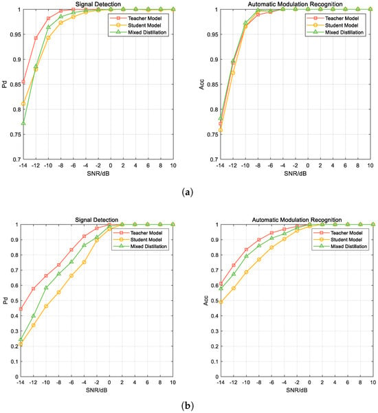
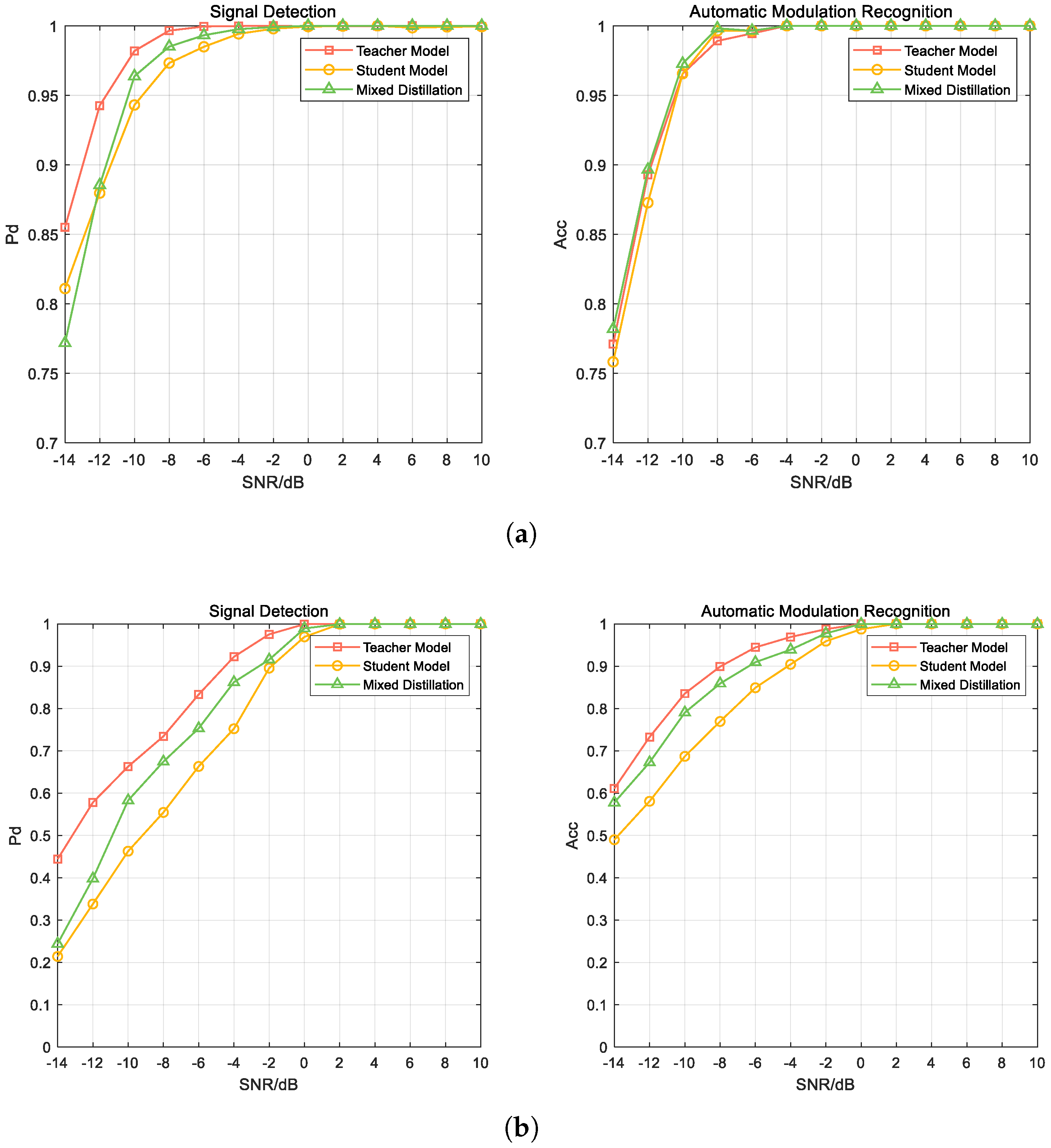
Using the teacher model, JDMR-LNet was directly trained, and the JDMR-LNet after distillation was used to predict data under different SNR (ranging from −14 dB to 10 dB); the prediction results are shown in Figure 4 and Table 3.

Figure 4. Teacher model, JDMR-LNet directly trained and JDMR-LNet after mixed distillation’s prediction results under different SNR. Figure (a) shows the results with only Gaussian noise added, while Figure (b) presents the results trained on the dataset incorporating spurious and missing pulses.

Table 3. Prediction Results. The signal detection probability and modulation recognition accuracy of the directly trained teacher model, the directly trained JDMR-LNet, and the after-distillation JDMR-LNet under 0 to −14 dB.

	SNR/dB	0	−2	−4	−6	−8	−10	−12	−14	Average
SD	Teacher Model	99.96%	100%	99.98%	99.95%	99.65%	98.19%	94.26%	85.51%	97.18%
	JDMR-LNet	99.94%	99.79%	99.42%	98.49%	97.32%	94.30%	87.96%	81.09%	94.78%
	After Distillation	100%	99.91%	99.76%	99.32%	98.50%	96.37%	88.53%	77.17%	94.95%
	Performance Gain	+0.06%	+0.12%	+0.34%	+0.83%	+1.18%	+2.07%	+0.57%	−3.92%	+0.17%
AMR	Teacher Model	100%	100%	100%	99.45%	98.91%	96.55%	89.27%	77.09%	95.16%
	JDMR-LNet	100%	100%	100%	99.64%	98.73%	96.55%	87.27%	75.82%	94.86%
	After Distillation	100%	100%	100%	99.64%	99.82%	97.27%	89.64%	78.18%	95.57%
	Performance Gain	0%	0%	0%	0%	+0.18%	+0.72%	+2.37%	+2.36%	+0.71%
AMR & SD	Performance Gain	+0.02%	+0.04%	+0.11%	+0.28%	+0.51%	+1.17%	+1.77%	+0.27%	+0.52%

In the SD task, when the SNR is relatively high, the teacher model can effectively detect the signal, almost achieving a 100% detection rate. When the SNR is greater than −10 dB, the Pd can be maintained above 0.95. However, for the directly trained JDMR-LNet, the detection performance is better at higher SNRs, but it significantly deteriorates when the SNR is below 0 dB. When the SNR is lower than −8 dB, the detection Pd has already dropped below 0.95. In the AMR task, the teacher model can maintain an accuracy above 0.95 when the SNR is −10 dB or higher, and even at an SNR of −12 dB, it can still achieve an accuracy of around 0.9. In contrast, the directly trained JDMR-LNet requires an SNR of at least greater than −10 dB to reach an accuracy of 0.95, and when the SNR is even lower, the ACC drops sharply, showing a significant gap compared to the teacher model. Clearly, the feature extraction capability of the student model, which has a simplified structure and fewer parameters, is weaker than that of the teacher model. This leads to a substantial decline in the Pd and accuracy compared to the teacher model at lower SNRs, with the maximum decrease being approximately 6%.

After distilling the JDMR-LNet using the method designed in this paper, the predictions made show a significant improvement compared to direct training. When the SNR is greater than −10 dB, both the correct probabilities for SD and AMR exceed 0.95, which is much higher than the accuracy of the JDMR-LNet trained directly, and is very close to the accuracy of the teacher model’s predictions, with a difference of about 1%. For the SD task, when the SNR is at 0 to −12 dB, the prediction accuracy of the distilled JDMR-LNet shows an average improvement of 0.73% in PD compared to the directly trained JDMR-LNet. In the AMR task, when the SNR is below −8 dB, the Acc of the distilled JDMR-LNet shows an average improvement of 0.90% compared to the directly trained JDMR-LNet.

When the SNR is high, input data detection and recognition are relatively easy. Even the directly trained JDMR-LNet can perform well in SD and AMR, so the improvement brought by distillation is not obvious. As the SNR gradually decreases, the performance gap between JDMR-LNet and the teacher model begins to emerge, and the improvement brought to JDMR-LNet by distillation also gradually increases. In the SD task, the maximum improvement is 2.07% at −10 dB, and in the AMR task, the maximum improvement is 2.37% at −12 dB. As the SNR continues to decrease, the difficulty of the SD and AMR tasks further increases. At this time, even the accuracy of the teacher model significantly decreases, which relatively narrows the gap between JDMR-LNet and the teacher model. The effective knowledge that JDMR-LNet can learn from the teacher model through distillation also decreases, and the performance improvement brought by distillation gradually declines. When the SNR decreases to −14 dB, LPI radar signals are severely submerged in background noise, which prevents the teacher network from extracting effective pulse features and yielding accurate SD predictions. The teacher network thus suffers significant performance degradation, with large prediction deviations and heavy noise contamination in its outputs. During distillation, the student network inevitably inherits not only valid knowledge but also the noise and prediction errors from the degraded teacher network. Under extremely low SNR, the transferred noise becomes dominant, so that the student network cannot distinguish effective features from interference. This directly lowers the prediction accuracy of the SD task and leads to negative distillation gain.

From the above results, it can be seen that the effect of distillation is very significant, which can bring great performance improvement to the lightweight JDMR-LNet model and significantly enhance its recognition results under low SNR. The impact of different distillation designs on the overall results during distillation will be discussed in the following sections.

4.3. Compare with SOTA

This section verifies the performance advantages of the proposed JDMR-LNet over the SOTA methods ETE [34] and RCDN [35] in SD and AMR tasks through quantitative comparisons. Experiments and comparative analyses were conducted across SNR levels ranging from 0 dB to −14 dB, as shown in Table 4.

Table 4. Comparison with SOTA Method.

	SNR/dB	0	−2	−4	−6	−8	−10	−12	−14
	JDMR-LNet	100%	99.91%	99.76%	99.32%	98.50%	96.37%	88.53%	77.17%
SD	ETE	91.60%	87.57%	82.72%	79.11%	71.76%	67.63%	59.71%	57.58%
	RCDN	96.60%	93.08%	89.76%	85.79%	79.56%	73.91%	69.07%	65.56%
	JDMR-LNet	100%	100%	100%	99.64%	99.82%	97.27%	89.64%	78.18%
AMR	ETE	100%	100%	100%	99.45%	96.36%	92.36%	85.09%	73.64%
	RCDN	100%	100%	100%	99.45%	96.91%	91.82%	87.82%	76.91%

In the SD task, JDMR-LNet demonstrates significant superiority across all SNR intervals: at 0 dB SNR, JDMR-LNet achieves an accuracy of 1.0, compared to 0.9160 for ETE and 0.9660 for RCDN. As noise interference intensifies (SNR decreases), the performance gap widens progressively. At the low SNR of −14 dB, JDMR-LNet achieves an accuracy of 0.7717, representing a 19% improvement over ETE (0.5758) and an 11% improvement over RCDN (0.6556), fully illustrating its robustness in weak signal detection.

In the AMR task, the performance is comparable between the two methods in the high SNR range (0 dB to −6 dB, both $\ge 0.9945$), but notable divergence emerges when SNR is below −8 dB. At −10 dB, JDMR-LNet achieves an accuracy of 0.9727, higher than ETE and RCDN; under extreme noise conditions of −14 dB, JDMR-LNet maintains a recognition rate of 0.7818, while ETE drops to 0.7364 and RCDN drops to 0.7691. This difference is attributed to JDMR-LNet’s attention distillation module, which precisely captures temporal modulation features.

In summary, JDMR-LNet exhibits superior comprehensive performance in complex noisy environments, particularly its robustness advantage in low SNR scenarios, validating its practical value in real-world radar signal processing applications.

4.4. Ablation Study

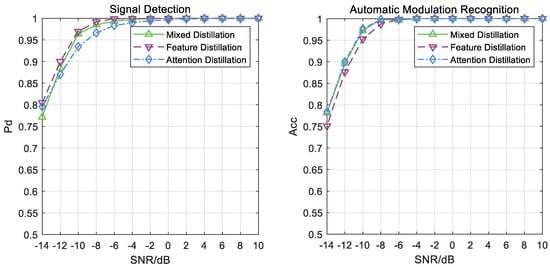
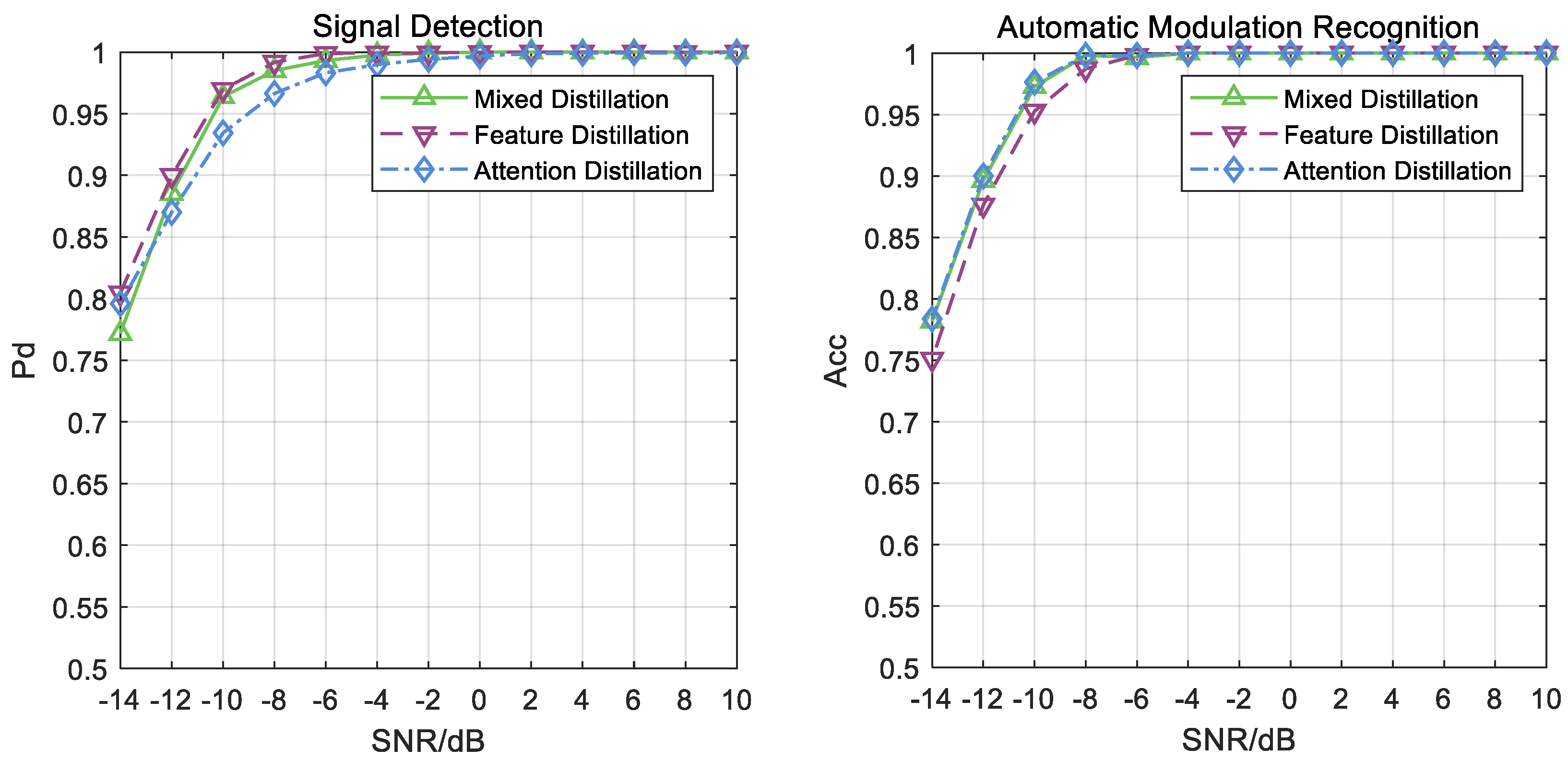
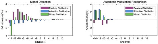
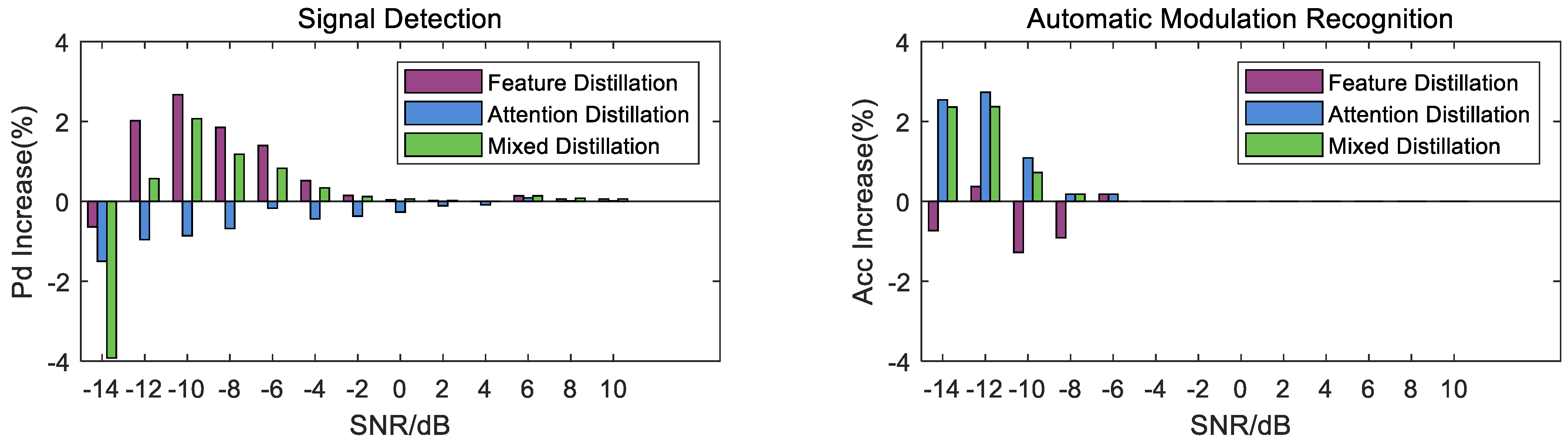
The distillation of JDMR-LNet employs different distillation methods for the task head and the attention head, combining both as the overall distillation method. To determine the impact of the feature distillation and attention distillation set in this paper on the overall distillation process and results, ablation experiments were conducted. The JDMR-LNet was trained separately using only the feature distillation and attention distillation components, and the results were compared with those of the mixed distillation. The results are shown in Figure 5 and Figure 6.

Figure 5. Results of using solely feature distillation, solely attention distillation, and mixed distillation methods. The green color represents the results using mixed distillation, the blue color indicates the results using attention distillation alone, and the purple color represents the results of feature distillation.

Figure 6. The performance improvement of different distillation methods compared to directly trained JDMR-LNet. In the SD task, attention distillation exerts a certain negative impact on the results, and this negative impact becomes more pronounced as the SNR decreases. By contrast, feature distillation can effectively improve the accuracy of the SD task after distillation. In the AMR task, attention distillation can significantly enhance the accuracy of the student network; however, since feature distillation is specifically designed for the SD branch, it exerts some negative impacts on the AMR task. Combining these two distillation methods obtains favorable distillation performance.

Effect of attention distillation: As shown in Figure 6, attention distillation can enhance the performance of small models across various SNRs in the AMR task. Specifically, when the SNR is below −8 dB, attention distillation can provide approximately a 2% performance improvement in the accuracy of AMR. However, for SD tasks, attention distillation adversely affects Pd after distillation, and this impact becomes increasingly pronounced as the SNR decreases.

Analyzing the structure of attention distillation, the reason for the performance enhancement is that through attention distillation, the attention layers of the student model and the teacher model exhibit similar attention mechanisms. This similarity helps to address the issue where the student model, due to its simpler structure, struggles to learn complex features and capture critical attention information. The output of the attention layer is provided simultaneously for the AMR task, which can improve the accuracy of the final results of AMR tasks.

Effect of feature distillation: As shown in Figure 6, feature distillation can significantly improve the accuracy of the SD task, and it reaches the highest at −10 dB. However, for AMR tasks, feature distillation reduces the accuracy of modulation type recognition, and its negative impact on AMR tends to increase as the SNR decreases.

The reason feature distillation can enhance the accuracy of signal detection is that the branching structure can map the area where the signal is located from the input of the task head. Therefore, the input of the task head contains some prior information about the area where the signal is located, which can improve detection accuracy. Since the small model uses the output of the attention layer to perform both SD and AMR tasks simultaneously, during backpropagation, the feature distillation of the branching structure causes the attention layer to focus more on the relationships of sequences over a broader range. In contrast, automatic modulation recognition requires the model to focus on the relationships of sequences within a narrower range, which leads to a negative impact on the AMR task.

Mixed distillation: The green curve in Figure 5 represents the results of training the small model using a combination of comprehensive attention distillation and branch structure feature distillation. Combined with Figure 6, it can be seen that its performance improvement of the two tasks is better than using attention distillation or feature distillation alone. In the SD task, the improvement in Pd achieved by mixed distillation at various SNRs is lower than that obtained by using attention distillation and feature distillation alone, with the highest improvement of 2.07% at −10 dB, but in the AMR task, it is much better than using feature distillation alone. In the AMR task, although mixed distillation has a slightly lower accuracy than using attention distillation alone, it can well balance the negative impact of attention distillation in the SD task.

Combining feature distillation and attention distillation allows the student model’s attention layers to learn the complex features extracted by the teacher model’s attention layers, while also enabling the student model’s task head to better learn the signal regions contained in the inputs of the teacher model’s task head. The synergy of these two approaches can lead to improved performance of the distilled JDMR-LNet model on both SD and AMR tasks.

4.5. Hyperparameter Analysis

This section focuses on conducting a systematic analysis of the impact of hyperparameters ($\gamma$ and $\rho$, T) on model performance in the experiment, aiming to determine the optimal hyperparameter configuration scheme adapted to the SD and AMR tasks in this study through quantitative experiments.

To maximize the manifestation of the impact of hyperparameter adjustments on model performance, we selected an SNR of −12 dB as the experimental benchmark. As verified by our previous experiments, the difference in core performance metrics between the teacher network and the student network is the most significant under this SNR. Subtle changes in hyperparameters are more intuitively reflected in performance fluctuations, which avoids the issues of performance saturation and insignificant hyperparameter influence that occur under high SNR conditions. The adjustments to hyperparameters are illustrated in the figure below. We fixed the hyperparameter $\gamma$ at 1 and adjusted the hyperparameter $\rho$ to obtain distillation results under different weight proportions. After comprehensive consideration, we selected $\gamma =1$ and $\rho =0.8$ as our final hyperparameters. At present, our research on hyperparameters is only preliminary, and more experiments can be conducted for further analysis in the future. The results are shown in Table 5.

Table 5. Experimental results with $\gamma$ set to 1 and different $\rho$ parameters.

$\mathit{\rho }$	0.1	0.2	0.3	0.4	0.5	0.6	0.7	0.8	0.9
SD	87.04%	87.82%	86.53%	87.19%	85.83%	87.61%	84.77%	88.53%	88.20%
AMR	89.18%	89.32%	89.64%	88.18%	89.09%	89.82%	87.82%	89.64%	90.00%

Regarding the distillation temperature T, we have also supplemented multiple distillation experiments conducted at different temperatures ranging from 1 to 9. Specifically, these experiments were carried out with fixed parameters of $\gamma =1$ and $\rho =0.8$, and the corresponding results are presented in Table 6.

Table 6. Experimental results with different distillation temperatures.

T	1	2	3	4	5	6	7	8	9
SD	88.00%	88.66%	88.56%	88.73%	88.53%	88.16%	88.23%	88.38%	88.07%
AMR	90.27%	89.18%	89.55%	89.61%	89.64%	89.27%	89.09%	89.18%	88.91%

It can be observed that the distillation temperature exerts a minimal influence on the experimental results; thus, a distillation temperature of 5 is adopted as the final experimental setup.

4.6. Model Complexity

After model lightweighting, the parameter quantities of the JDMR-LNet and the teacher model are shown in Table 7. The trainable parameters of the student model are approximately 11.04 times lower than those of JDMR-Net. The parameter quantity of the JDMR-LNet designed in this paper is significantly reduced compared to the original model, making it more suitable for deployment on resource-constrained platforms such as FPGA.

Table 7. The parameters and model size of JDMR-Net, the teacher model and JDMR-LNet. The compression ratio is the model size of the JDMR-LNet compared with the JDMR-Net and the teacher model.

	JDMR-Net	Teacher Model	JDMR-LNet	Compression Ratio (JDMR-Net)	Compression Ratio (Teacher Model)
Parameters	2,168,919	1,736,527	196,383	11.18	8.95
Model Size (MB)	8.27	6.62	0.74
Test Time (ms)	27.42	22.75	2.07

5. FPGA Deployment

5.1. Overall Architecture Design

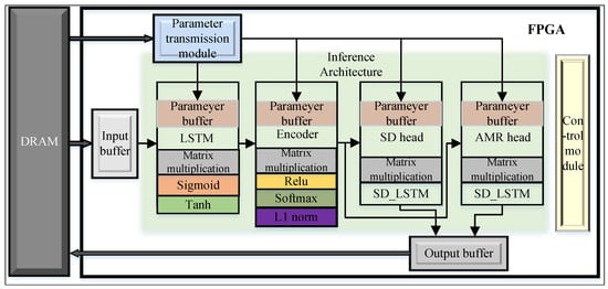
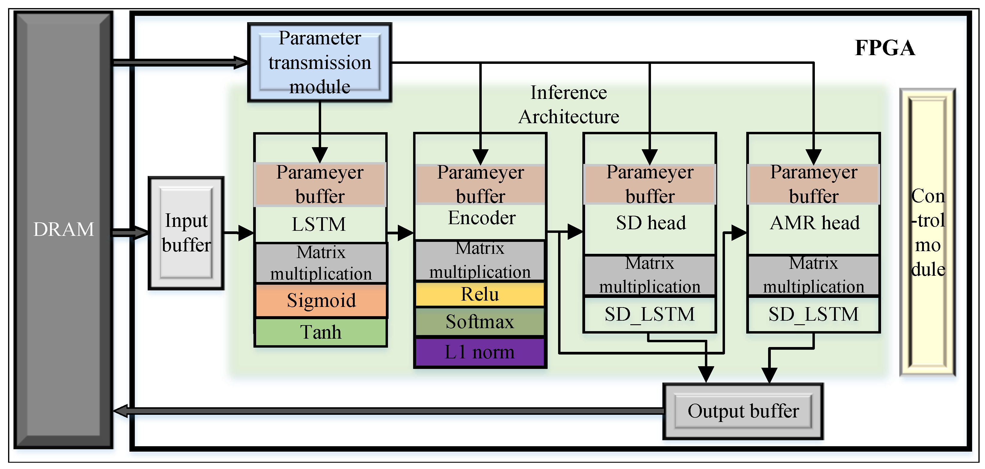
The overall architecture design of the lightweight model on the FPGA platform illustrated in Figure 7, forms a complete and efficient hardware operation chain. We have conducted functional simulations on this design to validate its operational logic and correctness. It relies on the collaborative data caching of the input buffer, parameter buffer, and output buffer and the efficient scheduling of the parameter transmission module and control module, as well as the core computing support of LSTM, Encoder, and task heads constructed with basic operation modules. This architecture achieves a significant optimization of hardware resource occupancy: compared with the original model, the parameter occupancy is reduced by 11.18 times, and the FPGA hardware storage resource occupancy is further reduced by 22.36 times. This achievement fully balances the lightweight requirements of the model and the hardware resource constraints of FPGA edge deployment, which not only verifies the rationality and efficiency of the architecture design but also lays a solid hardware foundation for the subsequent real-time and low-overhead radar signal processing tasks at the edge of radar systems.

Figure 7. The FPGA deployment framework design mainly consists of an external storage module (DRAM) and internal computing modules. DRAM is responsible for caching input data, weight parameters, and intermediate calculation results, providing data support for internal computing. The internal computing modules include LSTM, Encoder, SD Head, and AMR Head. All modules perform collaborative computing through an internal data bus.

For the network, input data, weight parameters, scaling factors, and matrix computation-related parameters (such as the number of rows and columns of the input matrix) are loaded from the off-chip DRAM into the on-chip buffers. The inference results of the network are first written into the on-chip output buffer, and finally stored in the off-chip DRAM.

The on-chip buffers consist of three types: input data buffer, parameter buffer, and output data buffer. Specifically: The input data buffer is used to cache input data transmitted from the off-chip DRAM. The parameter buffer is distributed within each network structural module, and serves to store weight parameters, scaling factors, and matrix computation-related parameters required for the inference of that specific module. The output data buffer is dedicated to storing the computation results of forward inference.

The inference architecture implements the forward inference operations of the model, and includes four inference sub-modules: LSTM, Encoder, SD head, and AMR head. Each inference sub-module incorporates computation modules such as matrix multiplication units, Sigmoid/Tanh activation modules, Softmax layers, and L1 normalization layers.

The parameter transmission module is responsible for reading model-related parameters from the off-chip memory and distributing these parameters to the parameter buffers within each inference sub-module. The control module manages the computation enable signals of all inference sub-modules throughout the entire computation process, and also controls the read enable signal of the parameter transmission module.

Communication between the modules is implemented using the AXI4-Stream protocol. AXI4-Stream is an interface protocol defined by ARM for high-speed data stream transmission, which can be used to connect a single master device (that generates data) to a single slave device (that receives data). The key control signals of the AXI4-Stream interface protocol are listed in Table 8 In the inference architecture, the output of each module is matrix data. In this study, matrix data is partitioned into blocks and transmitted via the AXI4-Stream protocol.

Table 8. AXI4-Stream interface protocol.

Signal	Description
aclk	Clock Signal
aresetn	Reset Signal
tready	Slave Ready to Receive Data
tdata	Master Transmitted Data
tstrb	Indicates Valid Bytes of TDATA
tlast	End of TDATA
tvalid	Data Transmission Valid
tuser	User-Defined Signal

5.2. Simulation Result

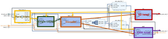
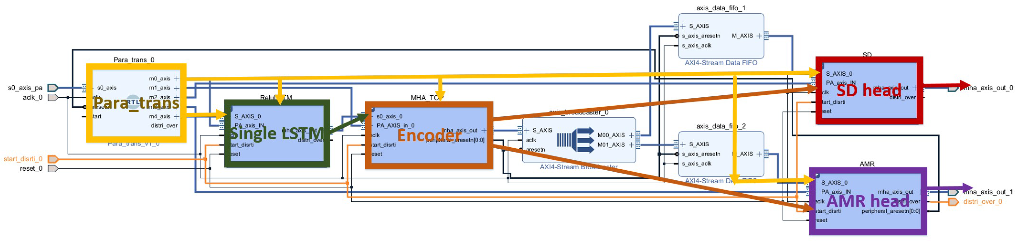
The implementation of the overall network architecture is illustrated in Figure 8. The data distribution module $Para\_trans$ reads out input data, weight parameters, and scaling factors from the external memory. The input data is sent to the input data buffer, while weight parameters and scaling factors are respectively delivered to the buffer of their corresponding network structures based on their affiliated network architectures.

Figure 8. The structural diagram of the block design implemented on the Vivado tool.

When the $\mathrm{start}\text{\_}\mathrm{distri}\text{\_}0$ signal goes high, each network structure redistributes the weight data in the buffer to its respective computational sub-modules. After the distribution of weight parameters and scaling factors across all structures is completed, the $\mathrm{distri}\_\mathrm{over}\_0$ signal is pulled high. Once $\mathrm{distri}\_\mathrm{over}\_0$ goes high, the input data is fed into the network for forward inference.

Due to the large parameter volume of the LSTM structure and the requirement for iterative computation in inference, the matrix multiplication module of this network structure necessitates a larger computation array. In this study, the size of the matrix multiplication array for LSTM within Single LSTM, $\mathrm{SD}\_\mathrm{head}$, and $\mathrm{AMR}\_\mathrm{head}$ is set to 16, while the size of all other matrix multiplication arrays is set to 4.

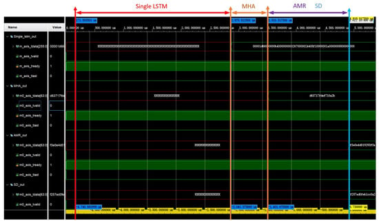
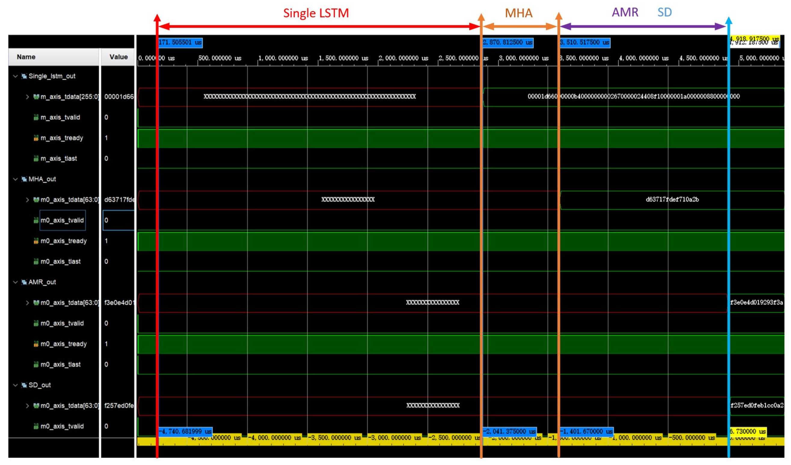
Vivado is employed as the simulation tool in this study. Parameters including input data, weights, and scaling factors are read from the Testbench file. The simulation waveform is illustrated in Figure 9, where the inference process of Single LSTM requires $5.39861\times {10}^6$ clock cycles; that of Encoder requires $1.27941\times {10}^6$ clock cycles; that of SD head requires $2.8168\times {10}^6$ clock cycles; and that of AMR head requires $2.80334\times {10}^6$ clock cycles. The simulation clock frequency settings, data throughput, and other related parameters can be found in Table 9.

Figure 9. The results of simulation and calculation conducted on the Vivado tool.

Table 9. Simulation Performance Metrics.

Clock Frequency	End-to-End Latency	Throughput
200 MHz	4.73 ms	633.58 k samples/s

The Xilinx XCZU9EG-2FFVB1156E FPGA chip is selected as the target device for the design, and the resulting synthesis results are presented in Table 10.

Table 10. FPGA resource utilization.

FPGA Resource	DSPs	BRAM	FF	LUT
Available Quantity	2520	912	548,160	274,080
Single LSTM	247	103.5	21,895	53,728
Encoder	508	151.5	26,864	66,909
SD head	232	72	20,962	41,335
AMR head	232	72	20,960	41,350
Total Resource Usage	1219	403	90,797	203,403
Total Utilization Rate	48.37%	44.19%	16.56%	74.21%

6. Conclusions

This paper proposes a lightweight integrated network for radar signal detection and recognition named JDMR-LNet, aiming to address prominent issues such as running high-complexity models on edge devices with limited computing resources. Based on the JDMR-Net model, this model significantly reduces the model volume by compressing the model structure and hidden layer dimensions, thereby lowering model complexity. Furthermore, to tackle the insufficient feature extraction capability of lightweight networks, this paper designs a branch-structured feature distillation method to enhance the signal detection performance of lightweight networks. The comprehensive use of feature distillation and relation distillation improves the overall performance of the model. Finally, the number of parameters of the network model is compressed by 11.04 times compared to the original model. Through distillation, under low signal-to-noise ratio conditions, it achieves a maximum performance improvement of 2.37% in the AMR task and 2.07% in the SD task. It successfully completes the task of a lightweight detection and recognition network and meets the target performance requirements.

Future research will focus on the deep integration of multi-source domain adaptation (MSDA) and dataset distillation (DD), combined with dataset dictionary learning to overcome the limitations of radar signal processing in complex scenarios [36,37,38,39]. This will provide an end-to-end solution for real-time radar processing in complex environments. On the other hand, since the current study is based on a simulated LPI radar dataset, future research will focus on verifying the method’s generalization ability in multi-scenario settings closer to practical applications, and take the optimization of the dynamic distillation strategy as one of the key research directions to further refine its adaptive adjustment mechanism for the variable requirements of complex scenarios, with bidirectional expansion from the dimensions of modulation modes and scenarios. By verifying the distillation, lightweighting performance of the method and the adaptation effect of the dynamic distillation strategy on the expanded datasets, the adaptability of the method in scenarios with complex signal types and intensive target interactions will be clarified, providing more comprehensive experimental support for its implementation in real radar systems.

References

- Liu, Y.; Xiao, P.; Wu, H.; Xiao, W. LPI radar signal detection based on radial integration of Choi-Williams time-frequency image. J. Syst. Eng. Electron. 2015, 26, 973–981. [Google Scholar] [CrossRef] [Scilit]
- Wang, D.; Cui, T.; Li, R.; Huang, Y.; Zhu, Y. Adaptive Broad Learning Network for LPI Radar Waveform Recognition. In Proceedings of the 2024 9th International Conference on Intelligent Computing and Signal Processing (ICSP), Xian, China, 19–21 April 2024; pp. 924–929. [Google Scholar] [CrossRef] [Scilit]
- Kong, S.H.; Kim, M.; Hoang, L.M.; Kim, E. Automatic LPI Radar Waveform Recognition Using CNN. IEEE Access 2018, 6, 4207–4219. [Google Scholar] [CrossRef] [Scilit]
- Tao, W.; Kaili, J.; Jingyi, L.; Tingting, J.; Bin, T. Research on LPI radar signal detection and parameter estimation technology. J. Syst. Eng. Electron. 2021, 32, 566–572. [Google Scholar] [CrossRef] [Scilit]
- Zhu, M.; Zhang, Z.; Li, C.; Li, Y. JMRPE-Net: Joint modulation recognition and parameter estimation of cognitive radar signals with a deep multitask network. IET Radar Sonar Navig. 2021, 15, 1508–1524. [Google Scholar] [CrossRef] [Scilit]
- Ye, H.; Li, G.Y.; Juang, B.H. Power of Deep Learning for Channel Estimation and Signal Detection in OFDM Systems. IEEE Wirel. Commun. Lett. 2018, 7, 114–117. [Google Scholar] [CrossRef] [Scilit]
- Geng, Z.; Yan, H.; Zhang, J.; Zhu, D. Deep-Learning for Radar: A Survey. IEEE Access 2021, 9, 141800–141818. [Google Scholar] [CrossRef] [Scilit]
- Qu, Z.; Hou, C.; Hou, C.; Wang, W. Radar Signal Intra-Pulse Modulation Recognition Based on Convolutional Neural Network and Deep Q-Learning Network. IEEE Access 2020, 8, 49125–49136. [Google Scholar] [CrossRef] [Scilit]
- Zhang, Z.; Li, Y.; Zhai, Q.; Li, Y.; Gao, M. Few-Shot Learning for Fine-Grained Signal Modulation Recognition Based on Foreground Segmentation. IEEE Trans. Veh. Technol. 2022, 71, 2281–2292. [Google Scholar] [CrossRef] [Scilit]
- Zhang, Z.; Zhu, M.; Li, Y.; Wang, S. JDMR-Net: Joint Detection and Modulation Recognition Networks for LPI Radar Signals. IEEE Trans. Aerosp. Electron. Syst. 2023, 59, 7575–7589. [Google Scholar] [CrossRef] [Scilit]
- Seng, K.P.; Lee, P.J.; Ang, L.M. Embedded intelligence on FPGA: Survey, applications and challenges. Electronics 2021, 10, 895. [Google Scholar] [CrossRef] [Scilit]
- Huang, M.; Luo, J.; Ding, C.; Wei, Z.; Huang, S.; Yu, H. An Integer-Only and Group-Vector Systolic Accelerator for Efficiently Mapping Vision Transformer on Edge. IEEE Trans. Circuits Syst. I Regul. Pap. 2023, 70, 5289–5301. [Google Scholar] [CrossRef] [Scilit]
- Buciluundefined, C.; Caruana, R.; Niculescu-Mizil, A. Model compression. In Proceedings of the 12th ACM SIGKDD International Conference on Knowledge Discovery and Data Mining, Philadelphia, PA, USA, 20–23 August 2006; pp. 535–541. [Google Scholar] [CrossRef] [Scilit]
- Lee, N.; Ajanthan, T.; Torr, P.H.S. SNIP: Single-shot Network Pruning based on Connection Sensitivity. arXiv 2019, arXiv:1810.02340. [Google Scholar] [CrossRef] [Scilit]
- Tai, C.; Xiao, T.; Wang, X.; E, W. Convolutional neural networks with low-rank regularization. In Proceedings of the 4th International Conference on Learning Representations, ICLR, San Juan, Puerto Rico, 2–4 May 2016; pp. 1–11. [Google Scholar]
- Vasu, P.K.A.; Gabriel, J.; Zhu, J.; Tuzel, O.; Ranjan, A. FastViT: A Fast Hybrid Vision Transformer Using Structural Reparameterization. In Proceedings of the IEEE/CVF International Conference on Computer Vision (ICCV), Paris, France, 2–6 October 2023; pp. 5785–5795. [Google Scholar]
- Sun, P.; Zhang, H.; Yang, J.; Wei, D. MobileViT Based Lightweight Model for Prohibited Item Detection in X-Ray Images. In Proceedings of the Asian Conference on Pattern Recognition, Kitakyushu, Japan, 5–8 November 2023; pp. 45–58. [Google Scholar]
- Müller, R.; Kornblith, S.; Hinton, G.E. When does label smoothing help? In Advances in Neural Information Processing Systems 32—NeurIPS 2019; Curran Associates, Inc.: Red Hook, NY, USA, 2019; Volume 32. [Google Scholar]
- Choudhary, T.; Mishra, V.; Goswami, A.; Sarangapani, J. A comprehensive survey on model compression and acceleration. Artif. Intell. Rev. 2020, 53, 5113–5155. [Google Scholar] [CrossRef] [Scilit]
- Cheng, Y.; Wang, D.; Zhou, P.; Zhang, T. A Survey of Model Compression and Acceleration for Deep Neural Networks. arXiv 2020, arXiv:1710.09282. [Google Scholar] [CrossRef] [Scilit]
- Gou, J.; Yu, B.; Maybank, S.J.; Tao, D. Knowledge Distillation: A Survey. Int. J. Comput. Vis. 2021, 129, 1789–1819. [Google Scholar] [CrossRef] [Scilit]
- Hinton, G.; Vinyals, O.; Dean, J. Distilling the Knowledge in a Neural Network. arXiv 2015, arXiv:1503.02531. [Google Scholar] [CrossRef] [Scilit]
- Romero, A.; Ballas, N.; Kahou, S.E.; Chassang, A.; Gatta, C.; Bengio, Y. FitNets: Hints for Thin Deep Nets. arXiv 2015, arXiv:1412.6550. [Google Scholar] [CrossRef] [Scilit]
- Zagoruyko, S.; Komodakis, N. Paying More Attention to Attention: Improving the Performance of Convolutional Neural Networks via Attention Transfer. arXiv 2017, arXiv:1612.03928. [Google Scholar] [CrossRef] [Scilit]
- Park, W.; Kim, D.; Lu, Y.; Cho, M. Relational Knowledge Distillation. In Proceedings of the IEEE/CVF Conference on Computer Vision and Pattern Recognition (CVPR), Long Beach, CA, USA, 15–20 June 2019; pp. 3967–3976. [Google Scholar]
- Liu, Y.; Cao, J.; Li, B.; Yuan, C.; Hu, W.; Li, Y.; Duan, Y. Knowledge Distillation via Instance Relationship Graph. In Proceedings of the 2019 IEEE/CVF Conference on Computer Vision and Pattern Recognition (CVPR), Long Beach, CA, USA, 15–20 June 2019; pp. 7089–7097. [Google Scholar] [CrossRef] [Scilit]
- Chen, P.; Liu, S.; Zhao, H.; Jia, J. Distilling Knowledge via Knowledge Review. In Proceedings of the IEEE/CVF Conference on Computer Vision and Pattern Recognition (CVPR), Nashville, TN, USA, 19–25 June 2021; pp. 5008–5017. [Google Scholar]
- Ren, S.; Wei, F.; Zhang, Z.; Hu, H. TinyMIM: An Empirical Study of Distilling MIM Pre-Trained Models. In Proceedings of the IEEE/CVF Conference on Computer Vision and Pattern Recognition (CVPR), Vancouver, BC, Canada, 18–22 June 2023; pp. 3687–3697. [Google Scholar]
- Hao, Z.; Guo, J.; Han, K.; Tang, Y.; Hu, H.; Wang, Y.; Xu, C. One-for-All: Bridge the Gap Between Heterogeneous Architectures in Knowledge Distillation. arXiv 2023, arXiv:2310.19444. [Google Scholar] [CrossRef] [Scilit]
- Vaswani, A.; Shazeer, N.; Parmar, N.; Uszkoreit, J.; Jones, L.; Gomez, A.N.; Kaiser, L.; Polosukhin, I. Attention is all you need. In Proceedings of the 31st International Conference on Neural Information Processing Systems, Long Beach, CA, USA, 4–9 December 2017; pp. 6000–6010. [Google Scholar]
- Zhang, Y.; Yang, Q. A Survey on Multi-Task Learning. IEEE Trans. Knowl. Data Eng. 2022, 34, 5586–5609. [Google Scholar] [CrossRef] [Scilit]
- Ranjan, R.; Patel, V.M.; Chellappa, R. HyperFace: A Deep Multi-Task Learning Framework for Face Detection, Landmark Localization, Pose Estimation, and Gender Recognition. IEEE Trans. Pattern Anal. Mach. Intell. 2019, 41, 121–135. [Google Scholar] [CrossRef] [Scilit]
- Kingma, D.P.; Ba, J. Adam: A Method for Stochastic Optimization. arXiv 2017, arXiv:1412.6980. [Google Scholar] [CrossRef] [Scilit]
- Scholl, S.; Panati, C.; Wagner, S. End-to-End Learning for Radar Electronic Support: Multi-label Classification and Explainable AI. IEEE Trans. Aerosp. Electron. Syst. 2025, 61, 11128–11140. [Google Scholar] [CrossRef] [Scilit]
- Bhavana, B.; Sabat, S.L. A Low-Complexity Deep Learning Model for Modulation Classification and Detection of Radar Signals. IEEE Trans. Aerosp. Electron. Syst. 2025, 61, 2548–2556. [Google Scholar] [CrossRef] [Scilit]
- Montesuma, E.F.; Stanc, S.L.; Mboula, F.N. Online Multi-Source Domain Adaptation through Gaussian Mixtures and Dataset Dictionary Learning. In Proceedings of the IEEE 34th International Workshop on Machine Learning for Signal Processing (MLSP), London, UK, 22–25 September 2024. [Google Scholar]
- Montesuma, E.F.; Ngolè Mboula, F.; Souloumiac, A. Multi-Source Domain Adaptation Meets Dataset Distillation through Dataset Dictionary Learning. In Proceedings of the ICASSP 2024—2024 IEEE International Conference on Acoustics, Speech and Signal Processing (ICASSP), Seoul, Republic of Korea, 14–19 April 2024; pp. 5620–5624. [Google Scholar] [CrossRef] [Scilit]
- Feng, H.; You, Z.; Chen, M.; Zhang, T.; Zhu, M.; Wu, F.; Wu, C.; Chen, W. KD3A: Unsupervised Multi-Source Decentralized Domain Adaptation via Knowledge Distillation. In Proceedings of the International Conference on Machine Learning, Virtual, 18–24 July 2021. [Google Scholar]
- Guo, F.; Wang, Y.K.; Qi, H.; Zhu, L.; Sun, J. DMSD-CDFSAR: Distillation from Mixed-Source Domain for Cross-Domain Few-shot Action Recognition. Expert Syst. Appl. 2025, 270, 126411. [Google Scholar] [CrossRef] [Scilit]
Disclaimer/Publisher’s Note: The statements, opinions and data contained in all publications are solely those of the individual author(s) and contributor(s) and not of MDPI and/or the editor(s). MDPI and/or the editor(s) disclaim responsibility for any injury to people or property resulting from any ideas, methods, instructions or products referred to in the content. |
© 2026 by the authors. Licensee MDPI, Basel, Switzerland. This article is an open access article distributed under the terms and conditions of the Creative Commons Attribution (CC BY) license.