


Abstract
This paper presents a dedicated dataset for the measurement and prediction of VHF signal propagation path error, aiming to mitigate their adverse effects on the ranging and positioning accuracy of terrestrial navigation systems. The Automatic Identification System (AIS), as a critical maritime collision-avoidance technology, enables terrestrial-based positioning using coastal AIS stations, offering significant advantages in terms of deployment and maintenance costs. However, propagation path error remains one of the primary sources of positioning inaccuracies, and no specialized datasets have yet been developed to support its systematic measurement and prediction. To address this limitation, a comprehensive data acquisition and processing framework for AIS-related VHF-band propagation path error is proposed. Based on this framework, a multidimensional dataset is constructed, incorporating temperature, relative humidity, air pressure, instantaneous wind speed, salinity, and measured propagation path error. The measured propagation path error data are collected using a self-developed additional secondary phase correction system. Hydrometeorological parameters obtained from authoritative sources at the same time and location are integrated with the measured data to form experimental samples with rich feature representations. Data cleaning and preprocessing procedures are further applied to improve dataset quality. The final dataset comprises 1,296,000 samples and is suitable for training and evaluating machine learning and deep learning models for VHF signal propagation path error prediction, thereby supporting enhanced positioning accuracy and the improved reliability of maritime navigation systems.
1. Introduction
Against the backdrop of accelerating economic globalization, maritime transportation has become one of the most efficient means for long-distance cargo transport, and its importance continues to grow [1]. At present, ship navigation relies predominantly on the Global Navigation Satellite System (GNSS). However, GNSS signals received onboard are inherently weak and based on openly accessible signal structures, making them highly vulnerable to interference, spoofing, and even complete denial [2]. When GNSS performance is degraded, ships may fail to obtain accurate positioning, navigation, and timing (PNT) information, posing serious risks to navigational safety. With the ongoing trend toward larger and faster vessels, reliance on a single navigation source can no longer meet the safety requirements of modern maritime transportation. This vulnerability is particularly pronounced in narrow waterways, congested ports, and adverse meteorological conditions, where positioning failures can significantly increase the likelihood of collisions and groundings [3]. Such incidents not only threaten the safety of crew members and assets, but may also trigger secondary consequences, including environmental pollution, cargo damage, and substantial economic losses [4,5]. Consequently, the development of terrestrial positioning and navigation systems that operate independently of space-based navigation systems has become a critical measure for enhancing the resilience of maritime navigation safety and is explicitly recommended by the International Maritime Organization (IMO) [6].
As the primary shipborne collision-avoidance system, the Automatic Identification System (AIS) is essentially a digital communication system that broadcasts both dynamic and static vessel information over the VHF band [7,8]. By enabling mutual identification and information sharing among vessels, AIS plays a critical role in ensuring navigational safety [9]. The positional information transmitted by AIS is obtained from its onboard GNSS receiver. However, GNSS inherently suffers from vulnerability to both intentional and unintentional interference, including signal anomalies, outages, blockage, spectrum congestion, and deliberate jamming or spoofing [10,11]. Consequently, exclusive reliance on GNSS poses significant risks to maritime navigation [12,13]. To mitigate these risks, the IMO has explicitly recommended and supported the deployment of dual-redundant positioning and navigation systems, integrating space-based and terrestrial-based solutions onboard vessels [14,15]. If shipborne AIS equipment can exploit signals transmitted from AIS shore stations for positioning, a reliable alternative can be provided in GNSS-degraded or GNSS-denied scenarios, thereby substantially enhancing navigational safety. Notably, this approach can fully leverage the globally deployed AIS shore-based infrastructure without requiring the construction of dedicated terrestrial navigation stations, leading to significant reductions in system deployment and maintenance costs. Moreover, as the International Convention for the Safety of Life at Sea (SOLAS) mandates AIS installation on the majority of commercial and fishing vessels, AIS-based positioning using shore-station time-of-arrival (TOA) or time-difference-of-arrival (TDOA) techniques does not require additional onboard navigation terminals, thus avoiding redundant equipment and further reducing implementation costs [16]. Due to these advantages, AIS-based terrestrial positioning has been recognized by both the IMO and the International Association of Marine Aids to Navigation and Lighthouse Authorities (IALA) as one of the most economically viable terrestrial positioning and navigation solutions currently available [17]. The positioning errors of terrestrial navigation systems mainly originate from three sources: reference station transmission error, signal propagation path error, and receiver-related error. This study focuses specifically on positioning errors induced by signal propagation effects. Fundamentally, positioning information in terrestrial navigation systems is derived from the propagation channel. When AIS signals in the VHF band propagate through the atmosphere and over the sea surface, their phase velocity is influenced by the propagation medium, resulting in deviations from the speed of light. If a constant light-speed assumption is adopted, non-negligible propagation delay errors are introduced. Accordingly, all propagation delay deviations from the speed of light are collectively defined as a propagation path error and considered for modeling and correction in this study. Despite their importance, the spatiotemporal characteristics of VHF signal propagation path error remain insufficiently investigated, which limits the achievable accuracy of high-precision terrestrial positioning systems. To address this limitation, this study aims to construct a high-quality VHF signal propagation path error dataset by integrating multisource hydrometeorological information, thereby providing a reliable data foundation for subsequent investigations using machine learning and deep learning methods to explore underlying spatiotemporal patterns and achieve accurate real-time error prediction.
Existing studies on AIS datasets have predominantly focused on vessel behavior analysis and trajectory prediction. For example, Andreas Tritsarolis et al. developed a standardized AIS database for large-scale maritime data analysis [18], covering more than 2.5 years of AIS records in the vicinity of the Port of Piraeus, Greece. This dataset integrates vessel position and static information with geographic and meteorological data, providing a comprehensive representation of operational conditions in busy port environments and supporting a wide range of maritime data analytics applications. In the same year, Clément Iphar et al. enhanced raw AIS data collected in the Brest region of France by extracting trajectory segments, labeling them according to their associated shipping routes, and identifying 17 maritime routes connecting regional ports [19]. The resulting dataset effectively supports maritime traffic modeling, analysis, and visualization tasks, thereby improving the feasibility and effectiveness of traffic monitoring applications. Subsequently, Rory Meyer et al. constructed an AIS dataset by aggregating spatial position and timestamp information from vessel reports [20]. Using a hexagonal grid representation, the dataset quantifies vessel dwell time and trajectory frequency across different months and vessel categories, and is openly shared through an open-source data processing workflow. Guelsoylu, Emre et al. further advanced AIS dataset construction by integrating shore-based camera imagery with corresponding AIS message data [21]. Through spatiotemporal alignment between YOLOv5-detected vessel bounding boxes and AIS-provided metadata—including vessel type, dimensions, heading, and speed—and by applying homography-based coordinate transformations, their dataset supports automatic vessel annotation, pose estimation, and the training and evaluation of maritime vision algorithms under diverse weather conditions. In addition, Shangbo Mao et al. developed a dedicated AIS database for trajectory prediction and data mining, systematically addressing trajectory cleaning, interpolation, and noise removal, and enabling applications such as maritime trajectory prediction, anomalous behavior detection, and traffic flow analysis [22]. Kapsar Kelly et al. utilized AIS data acquired from the exactEarth satellite constellation to construct a vessel activity dataset for the North Pacific Arctic region [23]. By filtering anomalous records and GPS-induced error and classifying vessels by type, this work filled a long-standing gap in high-resolution maritime activity data for the region. Despite these advances, existing AIS datasets primarily target vessel behavior analysis, trajectory modeling, and traffic monitoring, even when integrated with auxiliary data sources. In contrast, the accurate prediction of VHF signal propagation path error requires explicit consideration of hydrometeorological parameters influencing the propagation channel, as well as the combined effects of multiple propagation mechanisms, including direct propagation, reflection, scattering, and refraction. These mechanisms are highly sensitive to environmental conditions and differ fundamentally from the research objectives of the aforementioned studies. To capture the nonlinear spatiotemporal relationships between hydrometeorological factors and VHF signal propagation path error, machine learning and deep learning approaches offer promising solutions. However, the effectiveness of such methods critically depends on the availability of high-quality training datasets with rich and multidimensional input features. Therefore, this study aims to construct a dedicated dataset tailored to VHF signal propagation path error modeling and prediction.
In addition, the construction of such integrated datasets inevitably involves ethical and regulatory considerations that cannot be overlooked, particularly with respect to vessel trajectory privacy protection, the management of navigation-sensitive information, and compliance with international maritime data governance frameworks. Accordingly, clear data management and governance mechanisms must be established at the data acquisition stage to ensure that privacy and regulatory requirements are adequately addressed while preserving the scientific value of the dataset for ranging and positioning research. These challenges are primarily manifested during data acquisition and include the following:
- Conducting signal acquisition in a manner that avoids any disturbance or harm to the marine ecosystem, ensuring that high-frequency or high-intensity emissions do not pose potential risks to marine organisms;
- Safeguarding privacy in environmental data, by preventing unrestricted sharing of raw data within the research team;
- Implementing a compliant data protection plan to ensure that data collection, storage, and usage adhere to relevant regulations, such as the General Data Protection Regulation (GDPR), with respect to environmental data rights.
In this paper, the procedures for acquiring VHF signal propagation delay test signals and collecting hydrometeorological data are described. The collected data possess several notable characteristics:
- Adherence to established environmental ethics guidelines, with a focus on protecting ecological safety;
- Covers a wide range of environmental conditions, enhancing the completeness and reliability of the dataset.
- Application of standardized protocols and methods during data acquisition, ensuring consistency and quality;
- Compliance with relevant regulations, including the GDPR, guaranteeing lawful and ethical data handling.
The remainder of this paper is organized as follows. Section 2 presents the architecture and construction methodology of the VHF propagation path error dataset; Section 3 experimentally validates the effectiveness of the dataset for predicting VHF propagation path error; and Section 4 discusses the current limitations of the dataset and outlines directions for future work.
2. Structure of the VHF Signal Propagation Path Error Dataset
This paper presents a dedicated dataset for the investigation of VHF signal propagation path error, with its overall construction framework illustrated in Figure 1. The framework is composed of three main modules: a VHF signal propagation delay acquisition module, a data integration module, and a data cleaning module. This structure is designed to ensure the effectiveness and reliability of the dataset when applied to data analysis, feature extraction, and model training using machine learning or deep learning algorithms.
Figure 1.
Schematic diagram of the overall structure for constructing the VHF signal propagation path error dataset.
2.1. VHF Signal Propagation Delay Acquisition Module
This section focuses on the method for acquiring VHF signal propagation delay, including its design and implementation. The acquisition module is based on a self-developed additional secondary phase correction system [24], which enables the real-time measurement of VHF signal propagation delay. These measured values are compared with the calculated ideal propagation delays to derive the VHF signal propagation path error. The following provides a brief overview of the structural composition and measurement principles of the additional secondary phase correction system.
2.1.1. The Architecture and Measurement Principle of the Additional Secondary Phase Correction System
To meet the requirements for acquiring the measured VHF signal propagation delay, the authors’ research team independently developed an additional secondary phase correction system [24]. The system employs one transmitter to broadcast AIS signals and two receivers to simultaneously receive the signals and measure the propagation delay, thereby enabling the elimination of fixed system error. The overall dimensions of the system are 111 mm (height) × 482.6 mm (length) × 300 mm (width). A schematic diagram of the system architecture is shown in Figure 2, and a photograph of the physical system is presented in Figure 3. The transmitter subsystem mainly consists of a time synchronization module, a signal generation module, and a high-frequency power amplification module [24]. The time synchronization module consists of a rubidium atomic clock and a timing-grade GNSS receiver, which jointly maintain precise time synchronization between the transmitter and the receiver. After synchronization is achieved, both the transmitting and receiving units operate under the control of a synchronized pulse-per-second (PPS) signal, and the VHF signal propagation path error is measured with respect to this synchronized PPS reference. The timing-grade GNSS receiver provides PPS signals with an accuracy better than 20 ns and excellent long-term stability. However, its short-term stability is relatively poor. In contrast, the PPS output of a rubidium atomic clock exhibits outstanding short-term stability but suffers from limited long-term stability. To exploit the complementary advantages of both devices, the rubidium atomic clock is disciplined by the GNSS receiver, thereby enhancing its long-term stability while maintaining a highly stable PPS output. When GNSS signals are available, the GNSS-disciplined rubidium clock enables a time synchronization accuracy better than 10 ns. In the event of GNSS signal loss, the rubidium clock operates in free-running mode, during which the synchronization accuracy degrades to approximately 30 ns after about 24 h. Once GNSS signals are restored, the synchronization accuracy can rapidly recover to within 10 ns. As both the transmitting and receiving systems employ this GNSS-disciplined rubidium clock technique, the resulting high-stability and high-precision PPS synchronization pulses further improve the measurement accuracy of the VHF signal propagation path error. The signal generation module produces a periodic sequence with a length of 255 and a symbol rate of 10,200 bps, which is modulated using binary phase-shift keying (BPSK) to generate an intermediate-frequency signal at 455 kHz. Subsequently, the high-frequency power amplification module upconverts the 455 kHz intermediate-frequency signal to 160 MHz and amplifies the transmission power to 12.5 W for signal emission.
Figure 2.
Structural diagram of the additional secondary phase correction system for the propagation delay measurement.
Figure 3.
Hardware implementation of the transmitter and receiver in the additional secondary phase correction system.
The receiver subsystem mainly consists of a time synchronization module, a radio-frequency (RF) processing module, and a signal processing module. Similar to the transmitter, the time synchronization module employs a GNSS-disciplined rubidium atomic clock to achieve precise time synchronization with the transmitter. The RF processing module downconverts the received 160 MHz signal to an intermediate-frequency signal at 455 kHz. The signal processing module then performs analog-to-digital (AD) sampling of the intermediate-frequency signal, followed by baseband signal acquisition and tracking, to estimate the signal propagation delay.
During the actual data acquisition, Receiver A is fixed at a location very close to the transmitter (within 5 m), while Receiver B is deployed within a variable test area. The measured signal propagation delay from the transmitter to Receiver A and Receiver B are denoted as and , respectively, and can be expressed as follows [25]:
where denotes the propagation delay calculated based on the speed of light, and is expressed as: , where is the distance between the transmitter and Receiver A, and is the speed of light in vacuum; represents the additional propagation delay caused by the dielectric properties of the transmission medium; denotes the fixed equipment delay of Receiver A, which is determined by the intrinsic characteristics of the receiver hardware. Similarly, is the propagation delay computed based on the speed of light, where is the distance between the transmitter and Receiver B; denotes the additional delay due to the dielectric variation of the propagation medium along this path, and represents the fixed equipment delay of Receiver B, also determined by its internal hardware characteristics. Since Receiver A is located very close to the transmitter, the additional propagation delay can be neglected. Therefore, subtracting Equation (1) from Equation (2) yields:
Thus:
where is obtained through actual measurements using the additional secondary phase correction system, and are regarded as constant values derived from multiple measurements, the positions of the transmitter and Receiver A are precisely known, while the position of Receiver B can be precisely determined using real-time kinematic (RTK) positioning techniques. After obtaining the values within the test area, a correction model for VHF signal propagation path error is further established by jointly considering variations in the distance between the transmitter and receiver and the influence of environmental factors.
2.1.2. Presentation and Analysis of Measured VHF Signal Propagation Path Error
VHF signal propagation path error data were collected under real maritime environmental conditions. The transmitter was installed at the Lingjing Grand Hotel in Dalian, China (38.8404° N, 121.5179° E), while the two receivers were deployed at the Lingjing Grand Hotel and the Fujia Zhuang Shipping Hotel in Dalian, China (38.9273° N, 121.6478° E), respectively. The locations of the transmitter and receivers are illustrated in Figure 4.
Figure 4.
Locations of the receivers and transmitter.
The transmitter continuously broadcasts a predefined pseudo-random sequence. The receivers perform signal acquisition, tracking, and counter adjustment on the received signals, and output one measured VHF signal propagation delay value to the serial port every 10 s. In addition, the theoretical propagation delay was calculated based on the accurately known positions of the transmitter and receivers and the speed of light. The difference between the measured and theoretical delays was taken as the measured VHF signal propagation path error. Using data collected over a five-day period as an example (shown in Figure 5), the temporal and spatial variations of the VHF signal propagation delay and the corresponding path error are presented.
Figure 5.
Temporal variation of measured VHF signal propagation delay and path error: (a) Temporal variation of measured VHF signal propagation delay; (b) Temporal variation of measured VHF signal propagation path error.
Figure 5 illustrates the dynamic evolution of the VHF signal propagation delay and the corresponding path error over five consecutive days, from 17 July to 21 July. First, Figure 5a compares the measured propagation delay with the theoretical propagation delay. The data are presented at 10-s intervals, with 8640 samples collected per day, providing full 24-h coverage. Notably, the horizontal line at the bottom of the figure represents the theoretical propagation delay calculated using standard formulas. This value depends solely on the geographical distance between the transmitter and receiver and the speed of light in a vacuum, and under ideal conditions, it remains constant. In contrast, the colored fluctuating curves above correspond to the measured delay on different dates, which are consistently higher than the theoretical value and exhibit evident random variations.
Subsequently, Figure 5b removes the theoretical delay component to extract and display the real-time variations of the VHF signal propagation path error. A detailed analysis of Figure 5b reveals that the path error exhibited non-stationary fluctuations across different dates. Notably, on 20 July (green curve), the error fluctuated more drastically than on other days, with multiple high-frequency, large-magnitude instantaneous jumps observed throughout the day. In comparison, the variations on 17 July (black curve) and 18 July (red curve) were relatively moderate, with the error more tightly distributed.
This observation highlights the inherently dynamic nature of VHF signal propagation path error: it is not constant but is influenced by a complex interplay of multiple hydrometeorological factors. Therefore, constructing a multi-feature fused dataset that captures the nonlinear relationships between hydrometeorological variables and VHF signal path error is essential. Predictive models trained on such a dataset can accurately estimate the VHF propagation path error based on real-time hydrometeorological inputs, enabling the effective compensation of ranging deviations and improving the positioning accuracy of terrestrial navigation systems. This underpins the central aim of this study: to strengthen the data foundation for developing high-precision predictive models and to provide robust training and validation support.
2.2. Data Integration Module
This section aims to construct a dataset of VHF signal propagation path error. First, hydrometeorological observation data for the test sea area were obtained from the China Ocean Forecasting Network and the National Meteorological Science Data Center. The data were collected by a monitoring station at Dalian (38.9083° N, 121.64° E) with a sampling interval of 1 h, including variables such as station height, timestamp, temperature, relative humidity, precipitation, wind speed, wind direction, air pressure, salinity, horizontal visibility, weather phenomena, and total cloud cover. The timestamps were strictly aligned with the measured VHF signal propagation path error values recorded by the additional secondary phase correction system. Next, based on three propagation mechanisms—the two-ray propagation model, the tropospheric scatter model, and the evaporation duct model—key hydrometeorological parameters affecting the propagation path error were selected, namely temperature, relative humidity, air pressure, salinity, and instantaneous wind speed. Finally, the selected parameters were temporally interpolated to align with the sampling frequency of the VHF path error measurement, and the datasets were time-synchronized to generate a preliminary VHF signal propagation path error dataset.
2.2.1. Selection of Hydrometeorological Data
VHF signal propagation over the sea is primarily governed by the two-ray model; however, due to the presence of the troposphere and atmospheric ducts in the propagation environment, phase error induced by tropospheric-scattered signals and duct-refracted signals must also be considered.
- 1.
- Two-ray model: This model represents that the signal received at the receiver consists of a direct wave and a wave reflected off the sea surface. Accordingly, the received signal strength at the VHF frequency band used by AIS can be expressed as [26]:
As shown in Equation (7), the lower temperature/the higher salinity leads to increased electrical conductivity , resulting in a larger imaginary part of the relative permittivity . This causes the magnitude of the Fresnel reflection coefficient to become larger, thereby increasing the phase shift of the reflection coefficient . Consequently, the phase variation of the electromagnetic field intensifies, leading to greater propagation path errors for VHF signals.
On a rough sea surface, the sea-surface reflection coefficient is expressed as:
where denotes the Fresnel reflection coefficient, and denotes the roughness correction factor, which is a function of the root mean square height of the sea surface , and is expressed as:
where is the root mean square height of the sea surface, is the incidence angle, and is the first-kind zeroth-order Bessel function, and the root mean square height of the sea surface is a function of the sea surface wind speed, expressed as:
where denotes the wind speed at 10 m above the sea surface.
From Equation (10), it can be observed that a higher wind speed results in an increased root mean square height of the sea surface . This leads to an exponential decay in the magnitude of the roughness correction factor while simultaneously increasing the variance of the random phase fluctuations. Consequently, although the reflection intensity is attenuated, the phase uncertainty increases, causing larger phase fluctuations in the reflected signal. As a result, the VHF signal propagation path errors become more pronounced.
Based on the above analysis, under the two-ray model, the hydrometeorological parameters affecting the phase of the AIS received signal are temperature, salinity, and sea surface wind speed.
- 2.
- Tropospheric scattering model: When radio waves propagate through the troposphere with a non-uniform refractive index structure, path scattering occurs. In the generalized scattering model, the received AIS signal field strength is given by [27]:
- 3.
- Evaporation duct model: Due to the spatiotemporal inhomogeneity of atmospheric temperature, humidity, and pressure, the vertical distribution of the atmospheric refractive index becomes uneven, giving rise to atmospheric ducting that affects signal propagation. Among these, the evaporation duct is the most frequently occurring type of atmospheric duct. The received AIS signal strength can be represented using the wide-angle parabolic equation [28]:
As summarized, the hydrometeorological parameters affecting the phase velocity of AIS signal propagation are temperature, air pressure, relative humidity, instantaneous wind speed, and salinity.
2.2.2. Interpolation of Hydrometeorological Data
In this study, VHF signal propagation path data were collected at a sampling interval of 10 s, yielding a total of 8640 samples per day (from 00:00:00 to 23:59:50). In contrast, the hydrometeorological parameters—including temperature, relative humidity, air pressure, instantaneous wind speed, and salinity—were obtained from the Dalian site (38.9083° N, 121.64° E) provided by the China Marine Forecasting Network and the National Meteorological Science Data Center, where only hourly observations are available. As a result, each hydrometeorological parameter contains only 24 original values per day, leading to a clear mismatch in temporal resolution between the VHF signal propagation path error data and the corresponding hydrometeorological observations. To achieve spatiotemporal alignment between the measured VHF signal propagation path error and the hydrometeorological parameters, the Inverse Distance Weighting (IDW) method was employed for temporal interpolation of each hydrometeorological variable. Specifically, for each pair of adjacent hourly observations, 360 equally spaced data points were interpolated within the corresponding one-hour interval, with a temporal resolution of 10 s. Through this procedure, all hydrometeorological parameters were resampled to match the sampling interval of the VHF signal propagation path data, thereby ensuring consistent temporal resolution and effective spatiotemporal alignment between the two datasets. The rationale for selecting this method is detailed in [29].
IDW interpolation estimates the value at an unknown point as a weighted average of the observed values at surrounding known sample points, where the weights are inversely proportional to the distance between each sample point and the target location. Specifically, closer sample points are assigned greater influence. The method is expressed as:
where denotes the interpolated value of the hydrometeorological parameter at the target point; represents the index of the sampled data points used in the interpolation; is the observed value at the th sampling point; is the time difference between the target and the th sampling point; is typically set to 2; and is the number of sampling points involved in the interpolation, which was set to 2 in this study.
All interpolation procedures were strictly constrained within the physically reasonable ranges of each variable. The specific boundaries were determined based on the statistical distributions summarized in Table 1: temperature was limited to 15–30 °C, relative humidity to 45–96%, air pressure to 980–1100 hPa, instantaneous wind speed to 1.4–8.1 m/s, and salinity to 28.5–32 ‰. If any interpolated value exceeded the corresponding predefined range, boundary truncation was applied to prevent the introduction of nonphysical values. This strategy ensures the reliability, physical consistency, and numerical stability of the interpolated hydrometeorological parameters.
Table 1.
Descriptive statistical information of the experimental sample set.
2.2.3. Data Integration
The measured VHF signal propagation path error was paired with the corresponding hydrometeorological parameters recorded at the same time instants, forming a structured dataset comprising input features and target labels. This dataset included air pressure, temperature, relative humidity, instantaneous wind speed, salinity, and the measured VHF signal propagation path error. All variables were sampled at a uniform temporal resolution of 10 s, ensuring strict temporal alignment across all data streams. A summary of the experimental sample characteristics is provided in Table 1, and the feature correlation matrix for the dataset is visualized as a heatmap in Figure 6.
Figure 6.
Heatmap of feature correlations for the experimental dataset.
As summarized in Table 1, the air pressure ranged from 980 to 1100 hPa, with a mean value of 1040 hPa. The temperature varied between 15 °C and 30 °C (mean: 22.5 °C), while the relative humidity spanned 45% to 96% (mean: 70.5%). Instantaneous wind speed ranged from 1.4 to 8.1 m/s, with an average of 2.4 m/s. Salinity varied between 28.5‰ and 32‰ (mean: 29.3‰), and the measured VHF signal propagation path errors exhibited a range of 0.006 to 6.5 μs (mean: 2.78 μs). These statistical characteristics—comprising temperature, relative humidity, air pressure, instantaneous wind speed, salinity, and measured VHF signal propagation path errors—constitute the training dataset for modeling VHF signal propagation path error. This dataset provides a critical foundation for the subsequent analysis, modeling, and prediction of VHF signal propagation path errors.
Figure 6 presents a heatmap of feature correlations between five hydrometeorological parameters and the VHF signal propagation path errors. The results show that air pressure exhibited a s moderate-to-strong positive correlation with the path errors (r = 0.618), indicating that the VHF signal propagation path error increases with the rise in air pressure. Relative humidity also showed a moderate positive correlation (r = 0.524), meaning that a higher relative humidity is associated with a larger VHF signal propagation path error. In contrast, temperature demonstrated a moderate negative correlation (r = −0.434), which implies that the VHF signal propagation path error decreases as temperature rises. In comparison, instantaneous wind speed and salinity exhibited weak positive correlations with VHF signal propagation path errors (r = 0.292 and r = 0.310). This suggests that the increase in instantaneous wind speed and salinity will lead to a slight rise in the VHF signal propagation path errors, with the promoting effect being relatively insignificant. The quantitative correlation analysis results of the aforementioned characteristic parameters are consistent with the qualitative conclusions regarding the influence trends of each hydrometeorological parameter on the VHF signal propagation path errors presented in Figure 7, Figure 8, Figure 9, Figure 10 and Figure 11.
Figure 7.
The variation of VHF signal propagation path errors with temperature.
Figure 8.
The variation of VHF signal propagation path errors with relative humidity.
Figure 9.
The variation of VHF signal propagation path errors with air pressure.
Figure 10.
The variation of VHF signal propagation path errors with instantaneous wind speed.
Figure 11.
The variation of VHF signal propagation path errors with salinity.
Based on the feature correlation heatmap shown in Figure 6, the Pearson correlation coefficient matrix was obtained as follows:
In the matrix, the variables are ordered from left to right and from top to bottom as air pressure (P), relative humidity (RH), temperature (T), salinity (S), instantaneous wind speed (W), and propagation path error (E). The matrix reveals the linear correlation structure among the hydrometeorological parameters and their relationships with the VHF signal propagation path errors.
To systematically quantify the effects of hydrometeorological parameters on VHF signal propagation path errors, this section conducts a quantitative analysis at both the single-variable and multivariable interaction levels. First, the proportion of variance in the VHF signal propagation path errors explained by each individual variable is given by:
where denotes the coefficient of determination of the single variable; represents the proportion of variance in the VHF signal propagation path error explained by the corresponding hydrometeorological parameter through a linear relationship; denotes the hydrometeorological parameter; and represents the VHF signal propagation path error.
According to Equations (16) and (17), it can be concluded that air pressure exhibited the strongest positive correlation with the VHF signal propagation path error (rE,P = 0.618), with a variance explanation ratio of 0.382, indicating that air pressure is the most influential single factor affecting propagation path error. Relative humidity also showed a positive correlation with the propagation path error (rE,RH = 0.524), explaining 0.275 of the variance. Temperature demonstrated a moderate negative correlation (rE,T = −0.434), accounting for 0.188 of the variance. In addition, salinity exhibited a weak positive correlation with the VHF signal propagation path error (rE,S = 0.310), explaining 0.096 of the variance, while instantaneous wind speed showed a relatively weak correlation (rE,W = 0.292), contributing 0.085 to the explained variance. However, under strong wind conditions, instantaneous wind speed can indirectly amplify its influence on VHF signal propagation path errors by inducing increased sea-surface roughness.
Second, from the perspective of multivariable coupling, the proportion of variance in the VHF signal propagation path error jointly explained by multiple variables is given by:
where denotes the coefficient of determination for the multivariable case; denotes the proportion of variance in the VHF signal propagation path error explained by hydrometeorological parameter 1 through a linear relationship; denotes the proportion of variance explained by hydrometeorological parameter 2; and represents the proportion of variance associated with the covariance between hydrometeorological parameter 1 and hydrometeorological parameter 2.
Based on the calculation using Equation (18), when air pressure and relative humidity acted jointly, the proportion of variance in the VHF signal propagation path error explained was 0.492; for the joint effect of air pressure and temperature, the explained variance was 0.426. When air pressure and salinity acted together, the explained variance reached 0.418, while the joint contribution of air pressure and instantaneous wind speed explained 0.412 of the variance. For relative humidity and temperature acting jointly, the explained variance was 0.285; the combined effect of relative humidity and salinity explained 0.328 of the variance; and the joint contribution of relative humidity and instantaneous wind speed accounted for 0.335. In addition, the joint effect of temperature and salinity explained 0.212 of the variance, that of temperature and instantaneous wind speed explained 0.267, and the combined effect of salinity and instantaneous wind speed explained 0.179 of the variance.
2.2.4. The Influence of Hydrometeorological Parameters on VHF Signal Propagation Path Error
This section presents the influence of key hydrometeorological parameters—air pressure, temperature, relative humidity, instantaneous wind speed, and salinity—on VHF signal propagation path errors. In practical observations, these meteorological variables typically vary simultaneously. Therefore, an approximate control variable approach was adopted in this study. When analyzing the effect of a specific parameter, only samples in which the remaining four parameters exhibited minimal variation were retained and treated as approximately constant conditions (i.e., temperature variation < 0.4 °C, relative humidity variation < 0.4%, air pressure variation < 0.5 hPa, instantaneous wind speed variation < 0.1 m/s, and salinity variation < 0.1‰). Based on this approach, the influence of individual hydrometeorological parameters on propagation path errors was first analyzed (as shown in Figure 7, Figure 8, Figure 9, Figure 10 and Figure 11). Subsequently, the variation patterns of propagation path errors under coupled temperature–humidity effects were further investigated (as shown in Figure 12 and Figure 13).
Figure 12.
Effects of increasing temperature and decreasing relative humidity on VHF signal propagation path errors.
Figure 13.
Effects of increasing temperature and increasing relative humidity on VHF signal propagation path errors.
Figure 7 illustrates the temporal variation of VHF signal propagation path errors under the relative humidity of 70%, air pressure of 1000 hPa, instantaneous wind speed of 2.4 m/s, and salinity of 29.6‰, with temperature of 26 °C, 27 °C, and 28 °C, respectively. Overall, as the temperature increased, the VHF signal propagation path error exhibited a decreasing trend. At an identical time point, the propagation path error values at 28 °C were generally lower than those at 27 °C and 26 °C, indicating that higher temperature contributes to a reduction in propagation path errors. Detailed numerical results are provided in Table 2.
Table 2.
Numerical variation range of VHF signal propagation path errors with different temperature conditions.
Based on Table 2 and Figure 7, it can be concluded that temperature has an influence on the magnitude of VHF signal propagation path errors when relative humidity, air pressure, instantaneous wind speed, and salinity remain constant. From the overall variation trend of the data, lower temperature corresponds to a wider range of variation in the VHF signal propagation path errors. These experimental results are consistent with the theoretical inference described in Equation (11).
Figure 8 illustrates the temporal variation of VHF signal propagation path errors under the temperature of 23 °C, air pressure of 999.5 hPa, instantaneous wind speed of 1.7 m/s, and salinity of 30.1‰, with relative humidity levels of 86%, 88%, and 92%, respectively. Overall, the VHF signal propagation path error increased progressively with rising relative humidity. At an identical time point, the propagation path error values under 86% relative humidity were generally lower than those under 88% and 92%, indicating that lower relative humidity contributes to a reduction in propagation path errors. Detailed numerical results are provided in Table 3.
Table 3.
Numerical variation range of VHF signal propagation path errors with different relative humidity conditions.
Based on Table 3 and Figure 8, it can be concluded that relative humidity has an effect on the magnitude of VHF signal propagation path errors when temperature, air pressure, instantaneous wind speed, and salinity remain constant. From the overall trend of the data, lower relative humidity corresponds to a smaller variation range of the VHF signal propagation path errors. These experimental results are consistent with the theoretical inference described in Equation (11).
Figure 9 illustrates the temporal variation of VHF signal propagation path errors under the temperature of 25.5 °C, relative humidity of 80%, instantaneous wind speed of 2.4 m/s, and salinity of 30.1‰, with air pressures of 997 hPa, 1002 hPa, and 1005 hPa, respectively. Overall, the VHF signal propagation path error exhibited an increasing trend with rising air pressure. At an identical time point, the propagation path error values under 997 hPa were generally lower than those under 1002 hPa and 1005 hPa. Detailed numerical results are provided in Table 4.
Table 4.
Numerical variation range of VHF signal propagation path errors with different air pressure conditions.
Based on Table 4 and Figure 9, it can be concluded that air pressure has an influence on the magnitude of VHF signal propagation path errors when temperature, relative humidity, instantaneous wind speed, and salinity remain constant. From the overall trend of the data, lower air pressure corresponded to a smaller variation range of the VHF signal propagation path errors. These experimental results are consistent with the theoretical inference described in Equation (11).
Figure 10 illustrates the temporal variation of VHF signal propagation path errors under the temperature of 27 °C, relative humidity of 66.5%, air pressure of 1001 hPa, and salinity of 30‰, with instantaneous wind speeds of 1.8 m/s, 2.0 m/s, 2.4 m/s, 7.1 m/s, and 20 m/s (Under strong storm wind conditions), respectively. Overall, the VHF signal propagation path error increased progressively with increasing instantaneous wind speed. Detailed numerical results are provided in Table 5.
Table 5.
Numerical variation range of VHF signal propagation path errors with different instantaneous wind speed conditions.
By jointly analyzing Table 5 and Figure 10, it can be observed that under identical conditions of temperature, relative humidity, air pressure, and salinity, instantaneous wind speed exerted an influence on the VHF signal propagation path errors. As the instantaneous wind speed increased from 1.8 m/s to 2.4 m/s, the variation range of the VHF propagation path errors expanded. When the instantaneous wind speed further rose to 7.1 m/s, the propagation path errors range increased markedly to 5.38–6.41 μs, indicating that under moderate and higher wind speeds, sea surface disturbances begin to exert an effect on VHF signal propagation path errors. Furthermore, based on the statistically observed growth pattern of VHF signal propagation path errors within the interval where the instantaneous wind speed exceeded 7 m/s in the measured data, a data-driven simulation under strong storm conditions was constructed to examine the predictive adaptability of the proposed dataset under such extreme scenarios. First, within the constructed dataset, the variation in VHF signal propagation path errors with instantaneous wind speed was statistically analyzed for wind speeds greater than 7 m/s to characterize their growth behavior. Second, when the instantaneous wind speed exceeded 7 m/s, the sea surface transitioned into a rough-surface regime. Accordingly, a sea surface roughness correction factor was introduced to compensate for the prediction bias in VHF signal propagation path errors, and the statistically derived growth trend was extrapolated to strong wind conditions with an instantaneous wind speed of 20 m/s. Finally, while keeping the remaining hydrometeorological parameters unchanged, dynamic random perturbations were superimposed onto the measured VHF signal propagation path error data to generate simulated samples. As a result, the variation in VHF signal propagation path errors with instantaneous wind speed under strong storm conditions was obtained, as illustrated by the purple curve in Figure 10. The results indicate that under strong storm conditions with an instantaneous wind speed of 20 m/s, the VHF signal propagation path error ranges from 9.70 to 10.50 μs, which is significantly larger than that observed under smooth sea surface conditions. This demonstrates that VHF signal propagation path errors are subject to severe disturbances under strong storm conditions, leading to a substantial degradation in prediction reliability. Consequently, the proposed dataset is not suitable for modeling or predicting VHF signal propagation path errors under extreme weather conditions such as strong storms.
Figure 11 illustrates the temporal variation of VHF signal propagation path errors under the temperature of 26.5 °C, relative humidity of 68%, air pressure of 999 hPa, and instantaneous wind speed of 2.6 m/s, with salinity levels of 29.3‰, 29.6‰, and 30.1‰, respectively. Overall, the VHF signal propagation path error increased progressively with increasing salinity. At an identical time point, the propagation path error values under a salinity of 29.3‰ were generally lower than those under 29.6‰ and 30.1‰. Detailed numerical results are provided in Table 6.
Table 6.
Numerical variation range of VHF signal propagation path errors with different salinity conditions.
Based on Table 6 and Figure 11, it can be concluded that salinity has an influence on the magnitude of VHF signal propagation path errors when temperature, relative humidity, air pressure, and instantaneous wind speed remain constant. From the overall trend of the data, lower salinity corresponded to a smaller variation range of the VHF signal propagation path errors. These experimental results are consistent with the theoretical inference described in Equation (5).
Figure 12 illustrates the effects of the coupled variation of temperature and relative humidity on the VHF signal propagation path errors. Under conditions of the air pressure of 1004 hPa, the instantaneous wind speed of 3.1 m/s, and salinity of 30‰, the temporal variations of the VHF signal propagation path errors are shown for temperature and relative humidity pairs of (26 °C, 59%), (27 °C, 54%), and (28 °C, 50%), respectively. Overall, as temperature increases while relative humidity decreases, the VHF signal propagation path error exhibits a decreasing trend. The corresponding quantitative results are summarized in Table 7.
Table 7.
Variations in VHF signal propagation path errors with increasing temperature and decreasing relative humidity.
Table 7 and Figure 12 demonstrate the effects of the coupled interaction between temperature and relative humidity on the VHF signal propagation path errors under constant air pressure, instantaneous wind speed, and salinity. In conjunction with the conclusions drawn in Table 2 regarding the influence of temperature, higher temperatures are associated with smaller VHF signal propagation path errors. Under these conditions, a further reduction in relative humidity leads to an additional decrease in the propagation path error. This observation indicates that the combined effect of increasing temperature and decreasing relative humidity can effectively reduce the VHF signal propagation path error.
Figure 13 illustrates the effects of the coupled variation of temperature and relative humidity on the VHF signal propagation path errors. Under conditions of the air pressure of 1005 hPa, the instantaneous wind speed of 3.1 m/s, and the salinity of 30‰, the temporal variations of the VHF signal propagation path errors are shown for temperature and relative humidity pairs of (26 °C, 81%), (27 °C, 84%), and (28 °C, 86%), respectively. Overall, as temperature increases while relative humidity increases, the VHF signal propagation path error exhibits a increasing trend. The corresponding quantitative results are summarized in Table 8.
Table 8.
Variations in VHF signal propagation path errors with increasing temperature and increasing relative humidity.
Table 8 and Figure 13 illustrate the influence of the coupled interaction between temperature and relative humidity on the VHF signal propagation path errors under constant air pressure, instantaneous wind speed, and salinity. Consistent with the conclusions presented in Table 2, an increase in temperature generally leads to a reduction in the VHF signal propagation path error. However, when relative humidity increases simultaneously, the propagation path error increases accordingly. Moreover, the impact of temperature on the VHF signal propagation path error is weaker than that induced by relative humidity, indicating that relative humidity plays a more dominant role under these conditions.
2.3. Data Cleaning Module
To improve the quality of the VHF signal propagation path error dataset and ensure its reliability and validity for subsequent analysis, modeling, or applications, the integrated dataset was subjected to data cleaning. The data cleaning workflow is illustrated in Figure 14. This workflow includes steps such as dynamic imputation of missing values, hash-based detection of duplicate records, and sliding-window compensation for outliers.
Figure 14.
Data cleaning process.
- 1.
- For missing values in the VHF signal propagation path error dataset, a dynamic imputation method was employed. The algorithm proceeds as follows:
Step1: Valid value extraction. Search the feature columns of the VHF signal propagation path error dataset and construct a set of valid values, i.e.,:
where is the set of valid feature values for VHF signal propagation path error, denotes a valid feature value, and represents the missing value.
Step2: Imputation Strategy Selection. First, calculating the proportion of valid values :
where is the number of valid feature values in the VHF signal propagation path error dataset, and is the total number of feature entries.
When , the missing values are filled with the mean of the corresponding valid feature values, i.e.,:
where is the mean of the valid values for the corresponding feature, is the number of valid feature values in the VHF signal propagation path error dataset, and denotes each individual valid feature value.
When , the missing values are filled with the median of the corresponding valid feature values, i.e.,:
where is the median of the valid values for the corresponding feature, and is the number of valid feature values in the VHF signal propagation path error dataset.
Step3: Data Imputation. Replace the missing entries in the VHF signal propagation path error feature dataset with either the mean or the median of the valid values.
- 2.
- For duplicate entries in the VHF signal propagation path error dataset, a hash-based detection of duplicate algorithm is employed. The steps of the algorithm are as follows:
Step1: Feature fingerprint generation. For each record in the VHF signal propagation path error feature dataset, concatenate all feature values into a single feature vector and apply a hash function to generate a unique fingerprint, as shown in Equation (23):
where is the feature fingerprint generated via Equation (23), MD5 is a cryptographic hash function, represents the features contained in the th VHF signal propagation path error data record, and in this study.
Step2: Hash table construction. Record the hash values calculated in Step 1 into a hash map .
Step3: Duplicate detection. When the feature fingerprint of a new record already exists in the hash map, the record is identified as a duplicate.
Step4: Redundancy removal. Remove all duplicate records, retaining only one instance for each unique fingerprint. The resulting dataset constitutes the cleaned VHF signal propagation path error feature dataset, denoted as:
where denotes the cleaned VHF signal propagation path error feature dataset, and represents the VHF signal propagation path error feature record associated with a unique fingerprint.
- 3.
- For outliers in the VHF signal propagation path error dataset, the sliding-window compensation for outliers method is employed. The algorithm proceeds as follows:
Step1: Statistic calculation. Define the sample mean and sample standard deviation of all observations in the dataset as:
where is the th VHF signal propagation path error sample, and denotes the total number of VHF signal propagation path error samples.
Step2: Outlier detection. Identify and flag all data points that satisfy the condition .
Step3: Data correction. For each flagged outlier , if its temporal position satisfies (i.e., the distance from both the beginning and end of the dataset is no less than two sampling intervals), it is considered to have sufficient neighboring information. In such cases, the outlier is replaced using a five-point centered sliding window, which includes the two preceding points, the two following points, and the outlier itself, with the mean value calculated over these points:
where denotes the data value after mean-based replacement, and represents the original value of the outlier.
Step4: Direct removal. If an outlier is located within the first two () or last two () sampling intervals of the dataset, it lacks a complete set of neighboring observations required for reliable local estimation. In such boundary cases, the anomalous records are directly removed from the dataset to avoid introducing bias or distortion during subsequent analysis.
3. Model Verification
To evaluate the validity and usability of the constructed VHF signal propagation path error dataset in prediction tasks, seven models were selected: RNN, LSTM, Transformer, Regression Tree, Random Forest, ARIMA, and Linear Regression, representing deep learning models, traditional machine learning models, and classical statistical models, respectively, for systematic performance validation. The selection of these models balances the diversity of modeling paradigms with the comparability of results. RNN and LSTM, as classical time-series prediction models, are well-suited for capturing temporal dependency characteristics inherent in hydrometeorological sequences. The Transformer model, leveraging the self-attention mechanism, is capable of more effectively modeling complex dependency relationships between hydrometeorological parameter variables and VHF signal propagation path errors. Regression Tree and Random Forest models, as representative traditional machine learning approaches, possess a strong nonlinear fitting capability and a certain degree of interpretability, and have been widely applied in meteorological and environmental modeling tasks. The ARIMA model, as a typical statistical time-series method, provides strong modeling capability for linear temporal structures under stationary or weakly non-stationary conditions and serves as a baseline for assessing statistical predictability. Linear Regression, as a fundamental statistical modeling tool, is commonly used to characterize linear relationships between variables and likewise provides a reference benchmark for evaluating predictability from a statistical perspective. By comparing the performance of these diverse models in predicting VHF signal propagation path errors, the dataset’s adequacy in representing temporal information and its structural design can be comprehensively assessed. Moreover, from the perspectives of statistical modeling, traditional machine learning, and deep learning, the evaluation demonstrates the dataset’s effectiveness and usability in practical engineering prediction scenarios.
3.1. Dataset Preprocessing
All features contained in the dataset were used as model inputs in this study. During the preprocessing stage, the dataset was first standardized to ensure a consistent data format. Subsequently, the feature values of each column were normalized to eliminate the influence of differing feature scales on model training. Finally, the dataset was partitioned into a training set (60%), a validation set (20%), and a test set (20%) for model training and evaluation.
3.2. Hyperparameter Settings
This section presents the hyperparameter settings of the verification models. The specific configurations are summarized in Table 9, Table 10 and Table 11.
Table 9.
Hyperparameter Settings of Deep Learning Models.
Table 10.
Hyperparameter Settings of Machine Learning Models.
Table 11.
Hyperparameter Settings of Statistical Models.
Table 9 presents the architectures and hyperparameter settings of the three deep learning prediction models. Both RNN and LSTM adopt a single recurrent layer followed by a linear output layer, while the Transformer incorporates multi-head self-attention (MHA), a feedforward network (FFN), residual connections, and layer normalization. The input dimension for all three models was set to 6. RNN and LSTM each use a single hidden layer with 32 units. The Transformer employs a multi-head attention mechanism with 2 attention heads (nhead = 2) and a feedforward network dimension of 24 (d_ff = 24), along with residual connections and LayerNorm. All deep learning models use the Adam optimizer. The learning rate was set to 0.001 for RNN and LSTM, and 0.0001 for the Transformer. The batch size was 128, the number of training epochs was 50, and a dropout rate of 0.1 was applied to prevent overfitting.
Table 10 presents the architectures and hyperparameter settings of the two machine learning models. The regression tree relies on a single tree structure, achieving nonlinear fitting through decision and leaf nodes. The random forest is an ensemble method consisting of 100 regression trees, which improves robustness and generalization by averaging the predictions of multiple trees. For both models, the maximum depth was unrestricted (max_depth = None) to allow the trees to fully fit the training data. The minimum number of samples required to split a node (min_samples_split = 2) and the minimum number of samples required at a leaf node (min_samples_leaf = 1) were set to their default values to ensure fine-grained fitting.
Table 11 presents the structures and hyperparameter settings of the ARIMA and Linear Regression models. The ARIMA model consists of three components: autoregression (AR), differencing (I), and moving average (MA), with its core hyperparameters (p,d,q) selected and optimized based on the Akaike Information Criterion (AIC). During model construction, the differencing order d is first determined using the augmented Dickey–Fuller (ADF) test to ensure stationarity of the series. The optimal autoregressive order p and moving average order q are then automatically selected by minimizing the AIC value. The Linear Regression model constructs the predictive model as a linear combination of input features, with the regression coefficients estimated via the least squares method. The Linear Regression model does not rely on the autocorrelation structure of the time series; instead, it directly captures the linear mapping between input features (e.g., hydrometeorological parameters) and the prediction target, and requires no additional hyperparameter setting.
3.3. Experimental Results
For the input layers of the RNN, LSTM, Transformer, Regression Tree, Random Forest, ARIMA, and Linear Regression models, the training set was used to train the models, and hyperparameters were tuned based on the prediction performance on the validation set. Finally, the VHF signal propagation path errors were predicted on the test set, and the predictions of each model were compared with the observed propagation path errors to evaluate and validate their predictive performance. Figure 15 presents a comparison of the predicted and observed VHF signal propagation path errors across all models.
Figure 15.
Comparison chart of the measured and predicted values of the VHF signal propagation path error: (a) The comparison results of the RNN model; (b) The comparison results of the LSTM model; (c) The comparison results of the Transformer model; (d) The comparison results of the Regression Tree model; (e) The comparison results of the Random Forest model; (f) The comparison results of the Linear Regression; (g) The comparison results of the ARIMA.
As shown in Figure 15, the blue lines represent the observed VHF signal propagation path errors, while the red lines represent the predicted errors. Among the models, the Transformer achieved the best fit, with predicted values closely matching the observed values and exhibiting the smallest deviations. Although other deep learning and machine learning models showed some discrepancies, their predicted trends generally followed the observed variations, demonstrating the usability of the dataset across different predictive models. In contrast, Linear Regression and ARIMA performed poorly, with prediction curves unable to capture the complex error fluctuations. This is primarily due to the highly nonlinear spatiotemporal couplings present in the dataset, which exceed the linear representational capabilities of classical statistical models. To further assess the effectiveness of the constructed VHF signal propagation path error dataset in prediction tasks, quantitative metrics—including mean absolute error (MAE), root mean square error (RMSE), coefficient of determination (R2), and mean squared logarithmic error (MSLE)—were employed to evaluate the predictive performance of each model. The evaluation results are summarized in Table 12.
Table 12.
Evaluation Results of Quantitative Indicators for Different Prediction Models.
The evaluation results in Table 12 indicate significant differences in predictive performance among the models for VHF signal propagation path errors. The Transformer model demonstrated the best overall performance, achieving an MAE of 0.354 μs, RMSE of 0.634 μs, MSLE of 4.02 × 10⁻¹³ (all optimal values), and an R2 of 0.909, indicating high predictive accuracy and strong fitting capability when trained on the constructed dataset. In contrast, ARIMA and Linear Regression performed the worst, suggesting that classical statistical models struggle to capture the complex nonlinear relationships present in multifeature hydrometeorological data and are therefore unsuitable for such high-precision prediction tasks. Other models, such as LSTM and RNN, showed comparable performance, slightly inferior to Transformer but still better than traditional machine learning methods. Regression tree and random forest exhibited moderate modeling capability. However, their metrics were consistently lower than those of the deep learning models.
3.4. Model Generalization
To comprehensively evaluate the generalization capability of the models under different marine climatic conditions, test datasets were constructed along both spatial and temporal dimensions. In the spatial dimension, a synthetic test dataset for the South China Sea was generated based on the statistical characteristics and inter-variable correlations of the study dataset. Specifically, hydrometeorological parameter data—including temperature, air pressure, relative humidity, instantaneous wind speed, and salinity—were obtained from the China Marine Forecast Network and the National Meteorological Science Data Center. Using the multivariate linear relationships established between VHF signal propagation path errors and hydrometeorological parameters in the study dataset (as indicated by the feature correlation heatmap), the hydrometeorological parameter data were mapped to corresponding observed VHF signal propagation path errors, forming Test Dataset 1. In the temporal dimension, the model’s adaptability to other seasons in Dalian (e.g., spring, autumn, and winter) was further evaluated. Similarly, annual hydrometeorological parameter data—including temperature, air pressure, relative humidity, instantaneous wind speed, and salinity—were extracted from the same authoritative sources. Using the same error-generation mechanism, the corresponding VHF signal propagation path errors for each season were synthesized to form Test Dataset 2. Finally, Test Datasets 1 and 2 were separately fed into the Transformer model trained in Section 3.3, and the predictive results were quantitatively evaluated. The detailed performance metrics are summarized in Table 13 and Table 14.
Table 13.
Performance of the Transformer Model on Test Dataset 1.
Table 14.
Performance of the Transformer Model on Test Dataset 2.
As shown in Table 13 and Table 14, the Transformer model demonstrated strong predictive performance for both temporal generalization (Test Dataset 2) and spatial generalization (Test Dataset 1) tasks. For the temporal generalization task, the model achieved an MAE of 0.466 μs, RMSE of 0.692 μs, and R2 of 0.81. For the spatial generalization task, the corresponding metrics were an MAE of 0.511 μs, RMSE of 0.782 μs, and R2 of 0.70. Although there were slight differences between the two tasks, the overall error levels were low and the R2 values were above 0.7, indicating that the model can adapt to seasonal variations within the same region as well as effectively generalize to different marine environments. Moreover, the MSLE values were on the order of 10−13, further confirming the model’s stable ability to capture relative variations in VHF signal propagation path errors. These results fully demonstrate that the constructed dataset provides reliable generalization capability across both temporal and spatial dimensions.
4. Limitations
The VHF signal propagation path error dataset constructed in this study was primarily based on in situ measurements collected in the Dalian coastal waters of China, where the marine climate exhibits typical temperate monsoon characteristics, including pronounced seasonal variations in wind fields and distinct thermal–salinity structures. It should be explicitly noted that the dataset does not include observations under strong storm conditions (e.g., typhoons or severe convective events with instantaneous wind speeds exceeding 15 m/s). Data-driven simulations further confirm that the dataset is inherently unsuitable for modeling and predicting VHF signal propagation path errors under strongly disturbed meteorological conditions. Although preliminary spatial generalization capability was verified in Section 3.4 using a synthetic test dataset for the South China Sea, and good adaptability was observed in temporal transfer tasks across different seasons, the dataset still exhibited clear limitations in geographical and meteorological representativeness. On the one hand, substantial differences exist among marine regions in terms of hydrometeorological conditions, topography, and electromagnetic propagation environments. On the other hand, strong storm events can induce severe sea-surface roughening and abrupt variations in atmospheric refractivity—mechanisms that are not represented within the current data distribution. As a result, models trained on this dataset lack effective modeling capability under extreme weather conditions. To enhance environmental adaptability and practical applicability, future work will focus on expanding both the geographical coverage and the diversity of meteorological scenarios. Pilot observations are planned in multiple representative marine regions to systematically collect VHF signal propagation time delay measurements and corresponding hydrometeorological data across multiple regions, seasons, and climate types. In addition, numerical simulation techniques may be employed to generate synthetic data under diverse extreme climatic scenarios, further enriching the dataset’s diversity and representativeness. On this basis, a comprehensive dataset encompassing multiple regions, environmental conditions, and intensities of meteorological disturbance can be constructed, enabling systematic evaluation of model transferability under varying marine climates and ultimately advancing the application of VHF signal propagation path error prediction techniques to broader and more challenging marine environments.
5. Summary
This study constructed a high-quality dataset for the analysis, modeling, and prediction of VHF signal propagation path error, effectively addressing the lack of dedicated training data for high-precision ranging and positioning using machine learning or deep learning algorithms in AIS terrestrial navigation systems. Based on the identification of key hydrometeorological parameters influencing VHF signal propagation path error, the dataset integrates measured propagation path error data obtained from the authors’ self-developed additional secondary phase correction system with synchronous hydrometeorological observations (temperature, air pressure, relative humidity, instantaneous wind speed, and salinity). The final dataset comprises 1,296,000 samples and, through a systematic data cleaning workflow, ensures both reliability and usability for subsequent analysis and modeling tasks.
To evaluate the effectiveness of the constructed VHF signal propagation path error dataset for error prediction tasks, seven representative models were selected for comparative experiments. The results indicate that deep learning models can effectively capture the complex nonlinear relationships between multidimensional hydrometeorological parameters and VHF signal propagation path errors, demonstrating excellent predictive performance, with the Transformer model achieving the best results (MAE = 0.354 μs, RMSE = 0.634 μs, R2 = 0.909). In contrast, traditional statistical models, due to their simpler structures and lack of multivariate interaction modeling capability, struggled to accommodate the complex multifeature couplings present in the dataset. Importantly, in test scenarios designed for temporal generalization across different seasons and spatial generalization to a simulated South China Sea environment, deep learning models trained on this dataset maintained high predictive accuracy (R2 ≥ 0.70). These findings demonstrate that the dataset not only supports high-precision local modeling but also possesses strong cross-regional and cross-seasonal generalization potential.
In summary, this dataset provides a solid foundation for the deep learning-based prediction of VHF signal propagation path errors, significantly enhancing the ranging accuracy and robustness of terrestrial AIS systems. It establishes a critical technological basis for high-precision maritime navigation, intelligent ship collision avoidance, and maritime supervision applications.
Author Contributions
W.W. wrote the original draft and carried out the simulations. X.W. designed the measurement scheme and contributed to the writing of the paper. Z.Y. analyzed and compiled the data. X.S. arranged the architecture. Q.H. supervised the work. All authors have read and agreed to the published version of the manuscript.
Funding
This research was funded by the National Natural Science Foundation of China (No. 62301106), the Natural Science Foundation of Liaoning Province (2025-MSLH-092), and the Educational Commission of Liaoning Province of China (LJ212410151026).
Data Availability Statement
The data supporting the findings of this study are available from the corresponding author upon reasonable request.
Conflicts of Interest
The authors declare no conflicts of interest.
References
- Shang, T.Y.; Wu, H.; Wang, K.; Yang, D. Would the shipping alliance promote or discourage green shipping investment? Transp. Res. Part D Transp. Environ. 2024, 128, 104102. [Google Scholar] [CrossRef] [Scilit]
- Li, B.L.; Duan, J.L.; Chai, Y.H. Research on the Application of Vessel Track Data Based on AIS. Yangtze River Inf. Commun. 2021, 34, 30–33. [Google Scholar]
- Zhang, C.; Zou, X.; Lin, C. Fusing XGBoost and SHAP Models for Maritime Accident Prediction and Causality Interpretability Analysis. J. Mar. Sci. Eng. 2022, 10, 1154. [Google Scholar] [CrossRef] [Scilit]
- Gil, M.; Wrobel, K.; Montewka, J.; Goerlandt, F. A bibliometric analysis and systematic review of shipboard Decision Support Systems for accident prevention. Saf. Sci. 2020, 128, 104717. [Google Scholar] [CrossRef] [Scilit]
- Du, L.; Goerlandt, F.; Banda, O.A.V.; Huang, Y. Improving stand-on ship’s situational awareness by estimating the intention of the give-way ship. Ocean. Eng. 2020, 201, 107110. [Google Scholar] [CrossRef] [Scilit]
- Guo, X.; Wang, N.; Ren, Y.H. Ship trajectory segmentation by movement states while addressing uncertainty and sparsity. Ocean. Eng. 2024, 312, 119218. [Google Scholar] [CrossRef] [Scilit]
- Liu, Y.; Chen, X.H.; Zhang, R. An adaptive trajectory segmentation and simplification algorithm based on vessel behavioral features. Ocean. Eng. 2024, 312, 119329. [Google Scholar]
- Zhu, M.D.; Han, P.H.; Wang, C.L. An AIS Data-Driven Hybrid Approach to Ship Trajectory Prediction. IEEE Trans. Syst. 2024, 55, 96–109. [Google Scholar] [CrossRef] [Scilit]
- Liu, Z.H.; Qi, W.J.; Zhou, S.P.; Zhang, W.J.; Jiang, C. Hybrid deep learning models for ship trajectory prediction in complex scenarios based on AIS data. Appl. Ocean. Res. 2024, 153, 104231. [Google Scholar] [CrossRef] [Scilit]
- Liu, Z.H.; Qi, W.J.; Zhou, S.P.; Zhang, W.J.; Jiang, C. Low-complexity framework for GNSS jamming and spoofing detection on moving platforms. Iet Radar Sonar Navig. 2020, 14, 2027–2038. [Google Scholar]
- Wu, H.; Hu, L.Y.; Li, X.Y. A novel ship trajectory reconstruction approach based on low-rank tensor completion. Ocean. Eng. 2024, 310, 118724. [Google Scholar] [CrossRef] [Scilit]
- Huai, S.H.; Zhang, S.F.; Zhang, J. Holographic detection of AIS real-time signals based on sparse representation. EURASIP J. Wirel. Commun. Netw. 2019, 2019, 84. [Google Scholar] [CrossRef] [Scilit]
- Wang, X.Y.; Zhang, S.F.; Sun, X.W. Research on the Additional Secondary Phase Factor for Automatic Identification System Signals Transmitted over a Rough Sea Surface. Sensors 2018, 18, 617. [Google Scholar] [CrossRef] [Scilit]
- Kim, G.H.; Jeon, S.H.; Kim, C.W.; Han, D.W.; Kee, C.D. A combined numerical-empirical orbit propagation algorithm for satellite tracking and backup navigation system. In Proceedings of the Institute of Navigation International Technical Meeting 2012, ITM 2012, Newport Beach, CA, USA, 30 January–1 February 2012; pp. 812–819. [Google Scholar]
- Whelan, D.; Enge, P.; Gutt, G. Robust time transfer from space to backup GPS. In Proceedings of the 23rd International Technical Meeting of the Satellite Division of The Institute of Navigation (ION GNSS 2010), Portland, OR, USA, 21–24 September 2010; pp. 907–914. [Google Scholar]
- Jakub, T.; Jakub, H. GNSS Interference and Security: Impacts on Critical Infrastructure and Mitigation Strategies. Procedia Comput. Sci. 2025, 253, 2635–2644. [Google Scholar] [CrossRef] [Scilit]
- Resilient Position, Navigation and Timing (PNT). Available online: https://www.intertekinform.com/en-gb/standards/iala-g1180-2023-1345933_saig_iala_iala_3350493/ (accessed on 14 December 2023).
- Tritsarolis, A.; Kontoulis, Y.; Theodoridis, Y. The Piraeus AIS dataset for large-scale maritime data analytics. Data Brief 2022, 40, 107782. [Google Scholar] [CrossRef] [Scilit]
- Iphar, C.; Jousselme, A.L.; Pallotta, G. Maritime route and vessel tracklet dataset for vessel-to-route association. Data Brief 2022, 44, 108513. [Google Scholar] [CrossRef] [Scilit]
- Meyer, R.; Kleynhans, W.; Portier, M.; Beja, J.; Tyberghein, L. Dataset of ocean vessel traffic in the North Sea. Data Brief 2022, 51, 109746. [Google Scholar] [CrossRef] [Scilit] [PubMed]
- Gülsoylu, E.; Koch, P.; Yildiz, M.; Constapel, M. Image and AIS Data Fusion Technique for Maritime Computer Vision Applications. arXiv 2023, arXiv:2312.05270. [Google Scholar] [CrossRef] [Scilit]
- Mao, S.B.; Tu, E.M.; Zhang, G.H.; Rachmawati, L.; Rajabally, E. An Automatic Identification System (AIS) Database for Maritime Trajectory Prediction and Data Mining. In Proceedings of the ELM-2016, Singapore, 13–15 December 2016; Springer: Berlin/Heidelberg, Germany, 2017; pp. 241–257. [Google Scholar]
- Kapsar, K.; Sullender, B.; Liu, J.; Poe, A. North Pacific and Arctic marine traffic dataset (2015–2020). Data Brief 2022, 44, 108531. [Google Scholar] [CrossRef] [Scilit]
- Wang, X.Y.; Zhang, S.F.; Sun, X.W. The Additional Secondary Phase Correction System for AIS Signals. Data Brief 2017, 17, 736. [Google Scholar] [CrossRef] [Scilit] [PubMed]
- Sun, X.W.; Zeng, H.; Zhang, S.F. Measurement System for Additional Secondary Phase Factor of VHF Signal. CN Patent 201310368437, 11 December 2013. [Google Scholar]
- Wang, X.Y. Research on AIS Autonomous Positioning System Propagation Path Error and Correction Techniques. Dalian Maritime University 2018. Available online: https://kns.cnki.net/kcms2/article/abstract?v=yqBhao7Q9gxtqbX64okeVMjbxP40Iwypjgz2k97I9Jp_fSeS3Yb2BVWugFoQIRdfZbAuj66_FkQCUWi0YQoHLS9JcMya_cdEtt_YNezWIhRxR1qvCv-EeYwofXN-d8J8JC4FZ54sJWk2iy6Ohc19CSQxqsoEr1S0Ju6nJfZl4XP64cIUhmOKvzAPwaL9dOXZ&uniplatform=NZKPT&language=CHS (accessed on 16 November 2018).
- Zhang, M.G. Tropospheric scattering propagation. In Tropospheric Scattering Propagation; Electronics Industry: Beijing, China, 2004; pp. 103–112. Available online: https://xueshu.baidu.com/ndscholar/browse/detail?paperid=b7ae90cc30941222683795185f0fe652 (accessed on 1 October 2004).
- Dockery, G.D.; Kuttler, J.R. An Improved Impedance-Boundary Algorithm for Fourier Split-Step Solutions of the Parabolic Wave Equation. IEEE Trans. Antennas Propag. 1996, 44, 1592–1599. [Google Scholar] [CrossRef] [Scilit]
- Sheng, Y.; Yuan, Z.P.; Chen, Y.Q. Liaoning Provincial Township Weather Foreacasting Business System. J. Meteorol. Environ. 2008, 24, 13–17. [Google Scholar]
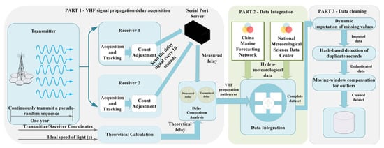
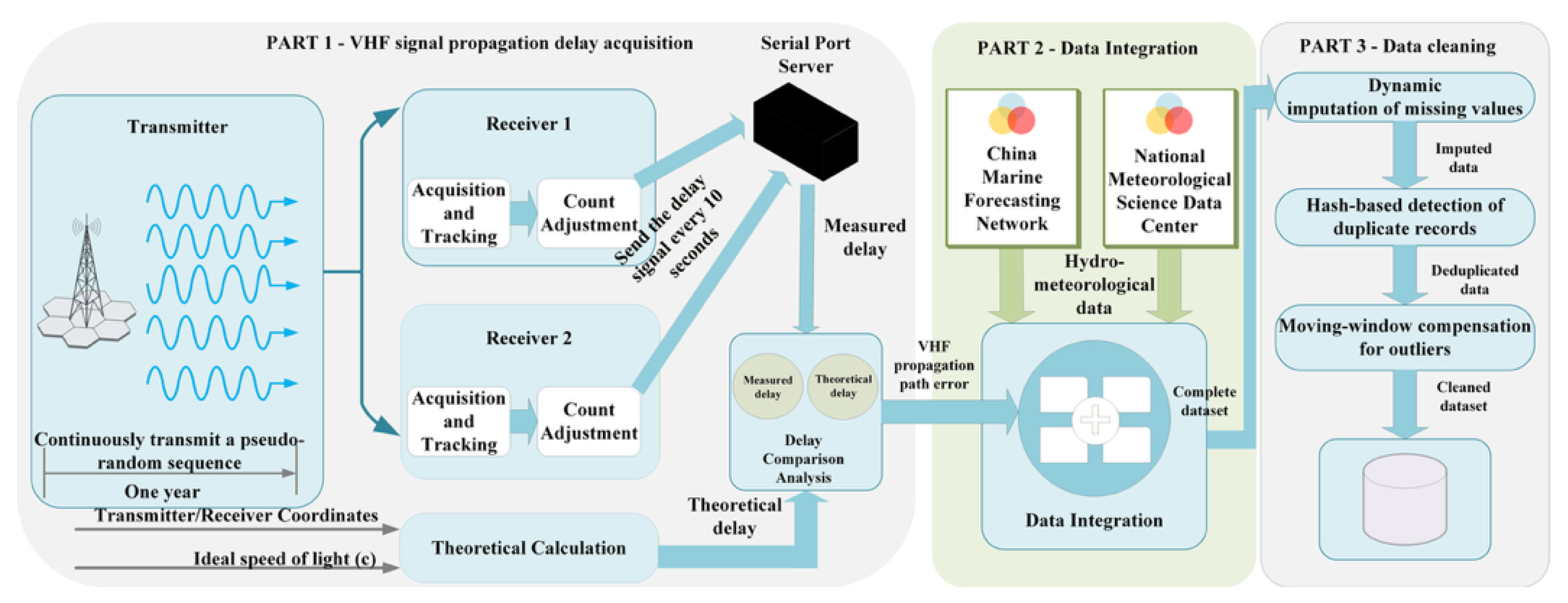
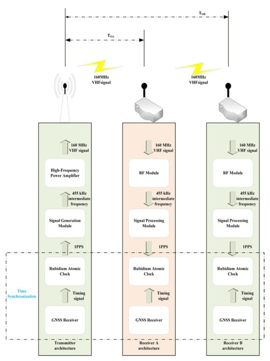
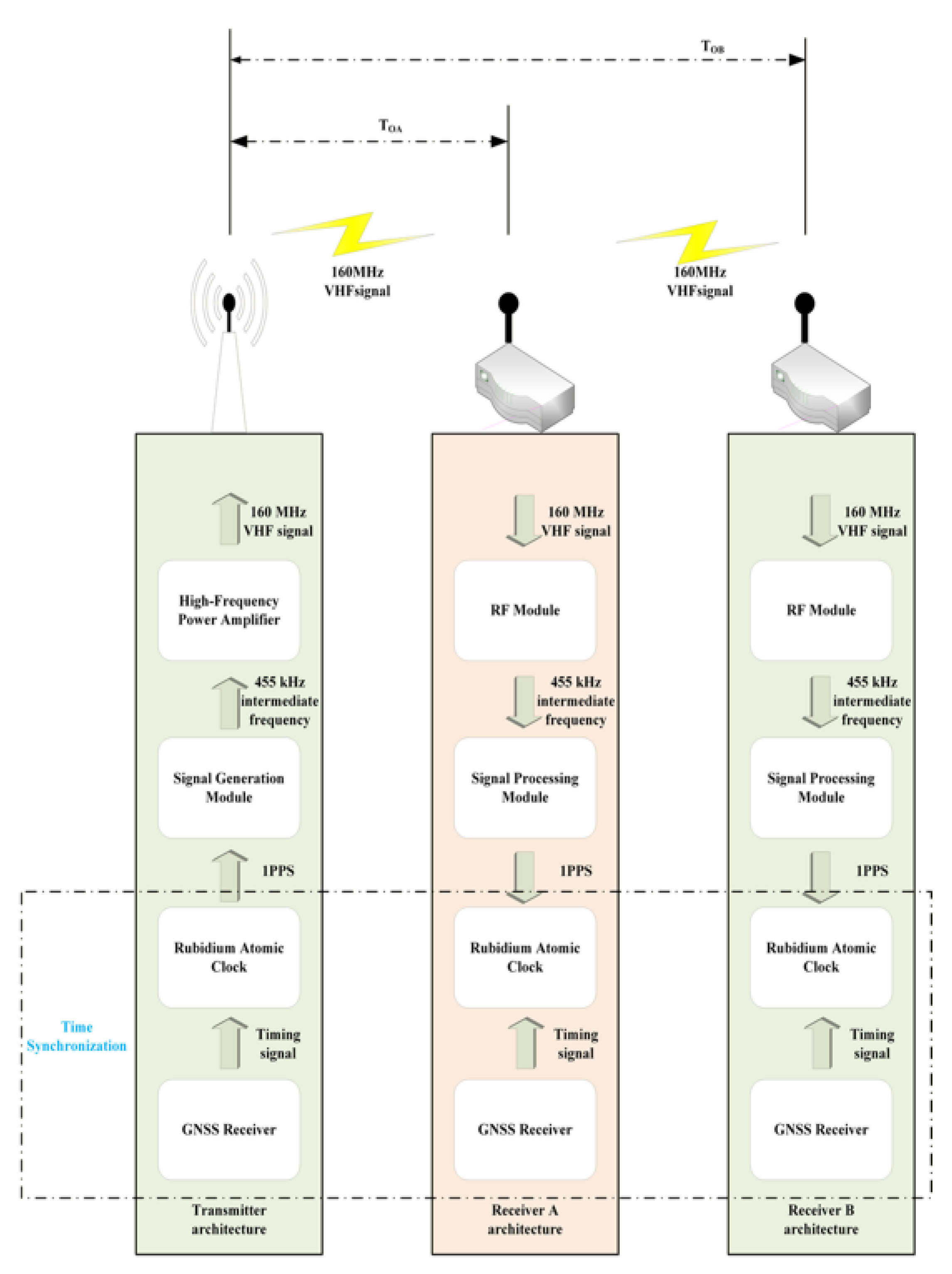
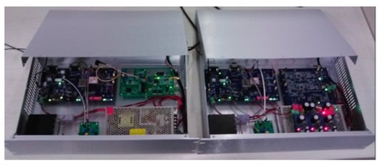
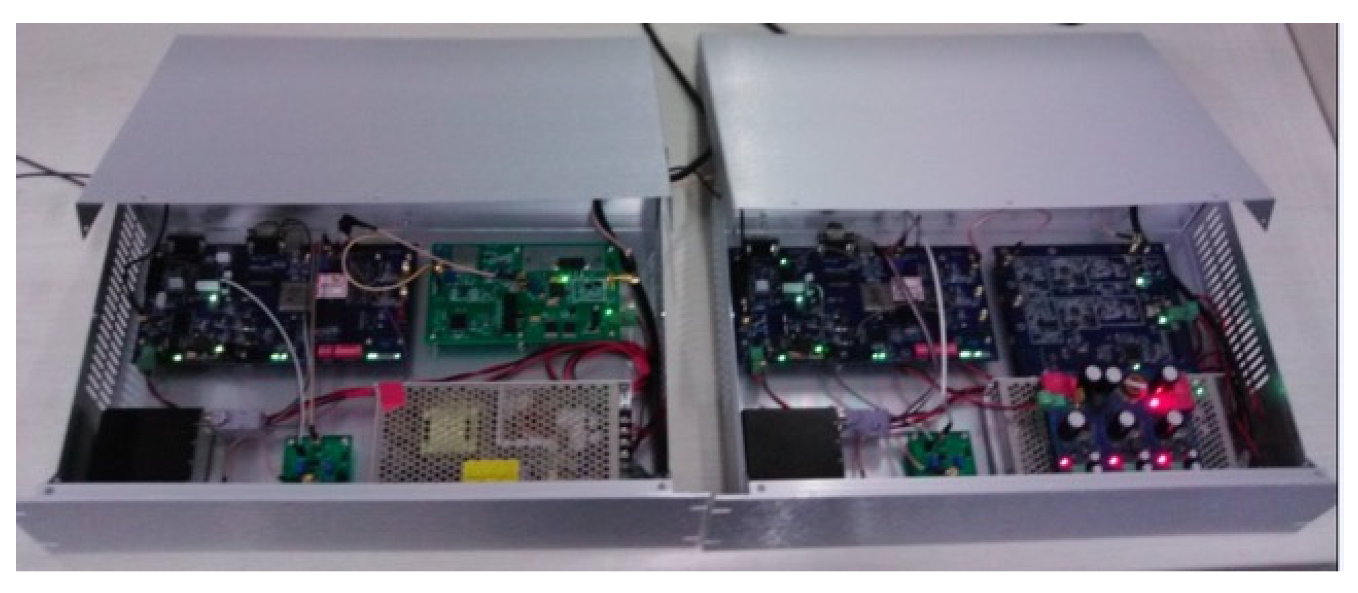
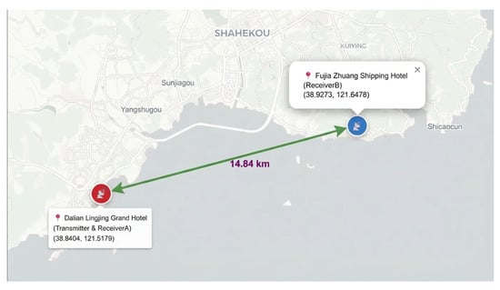
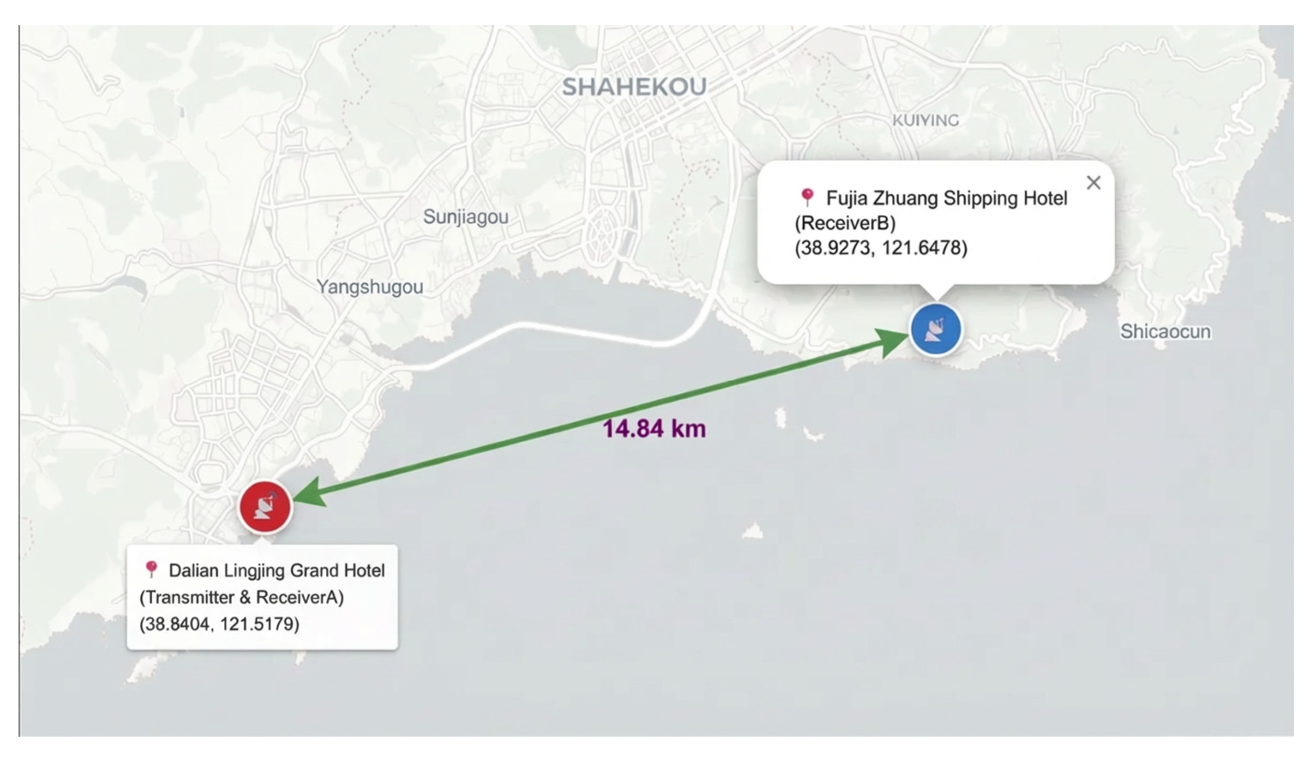
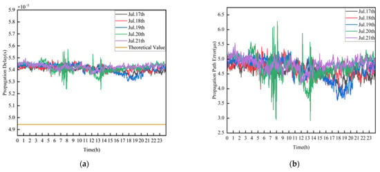
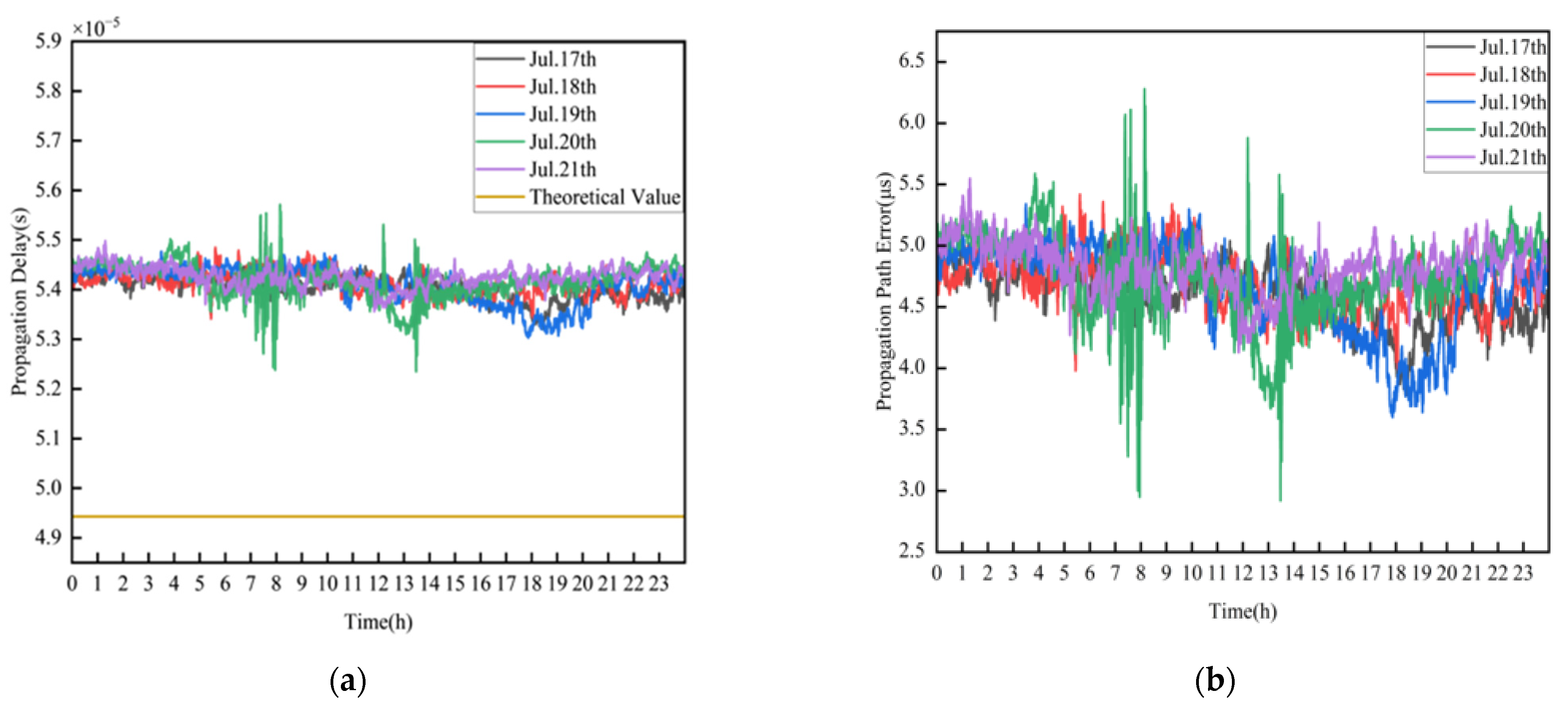
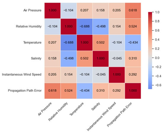
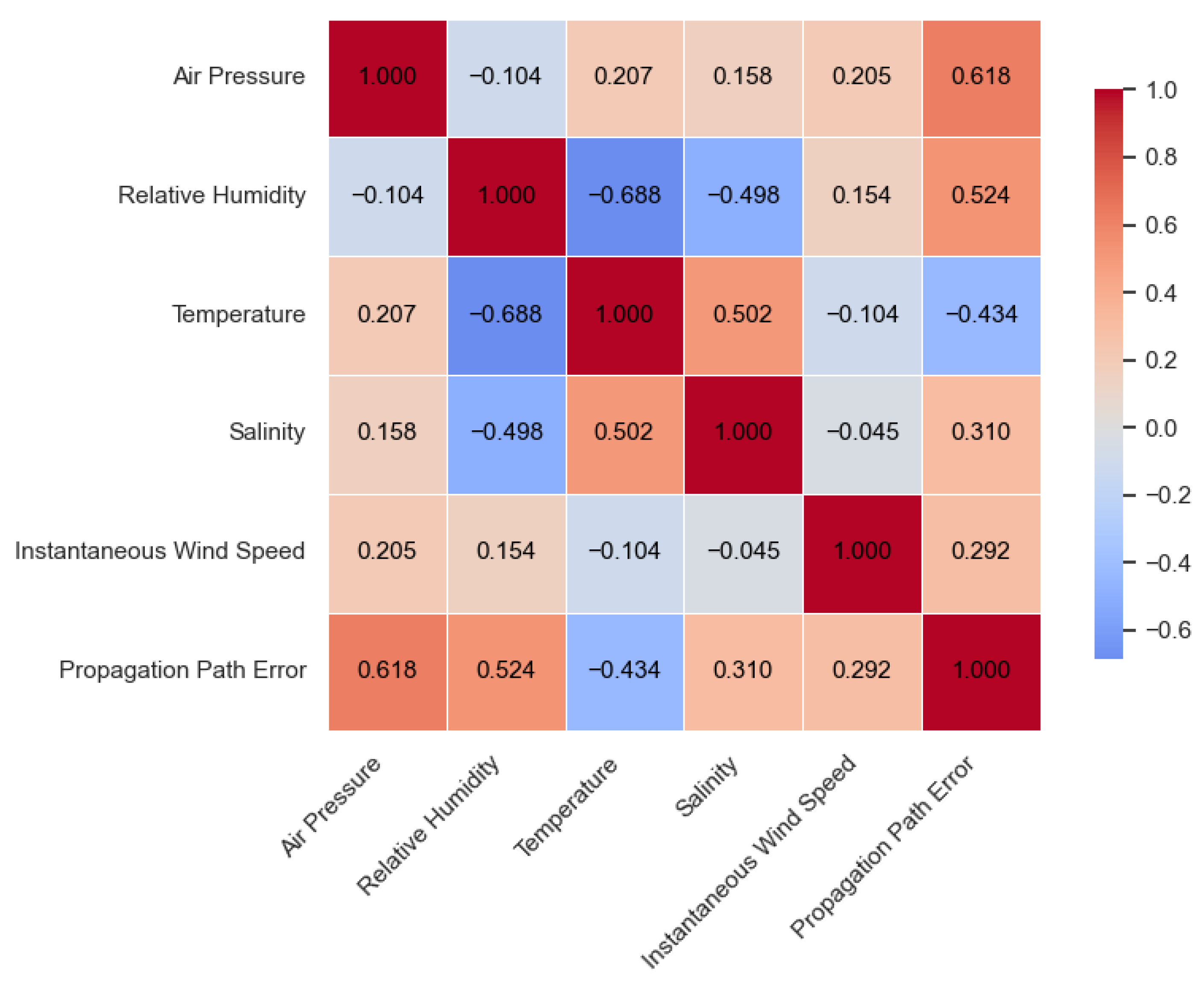
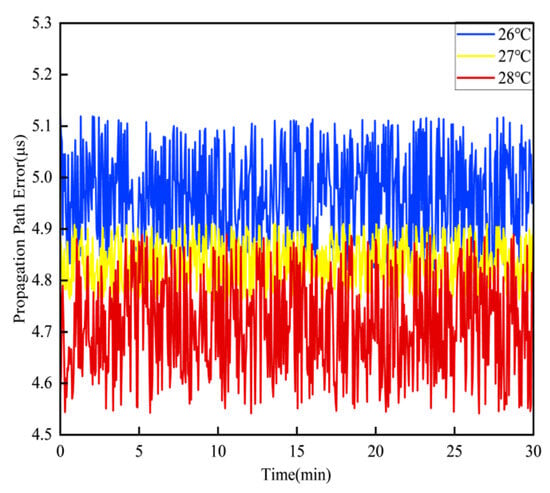
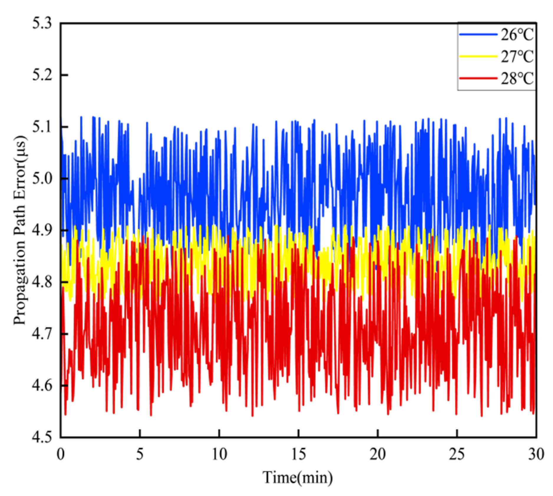
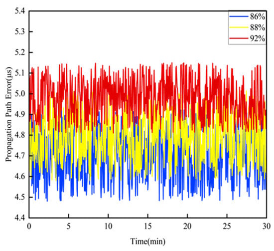
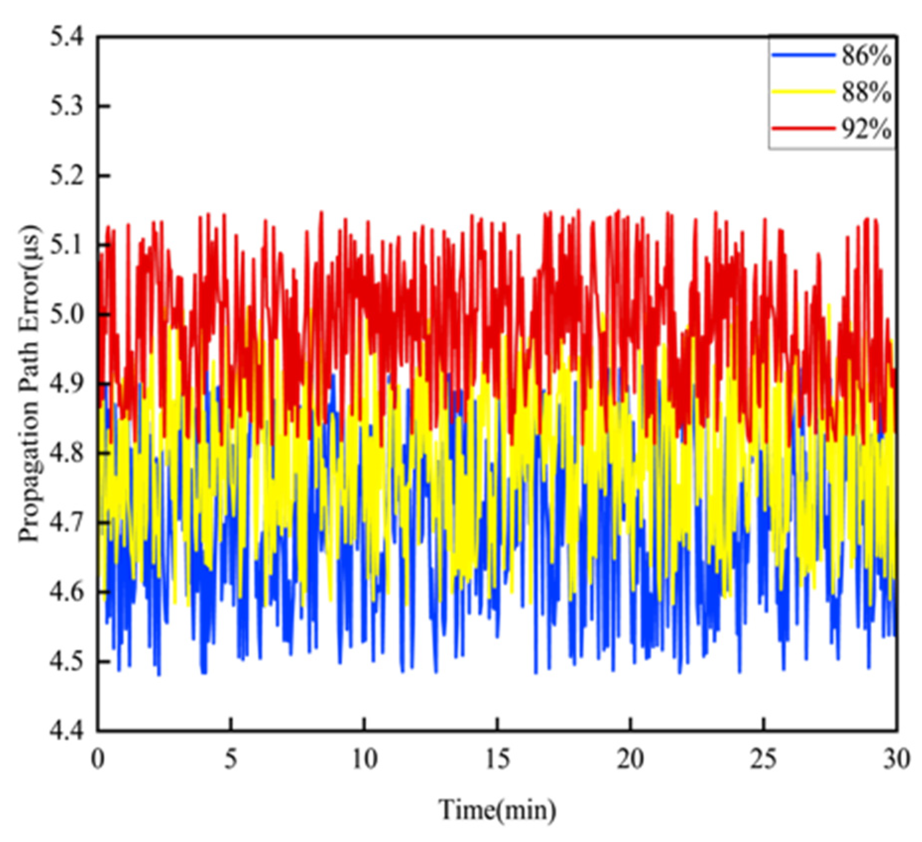
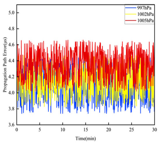
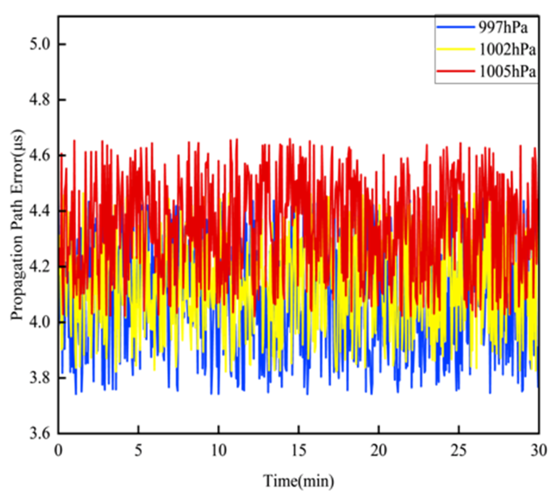
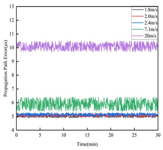
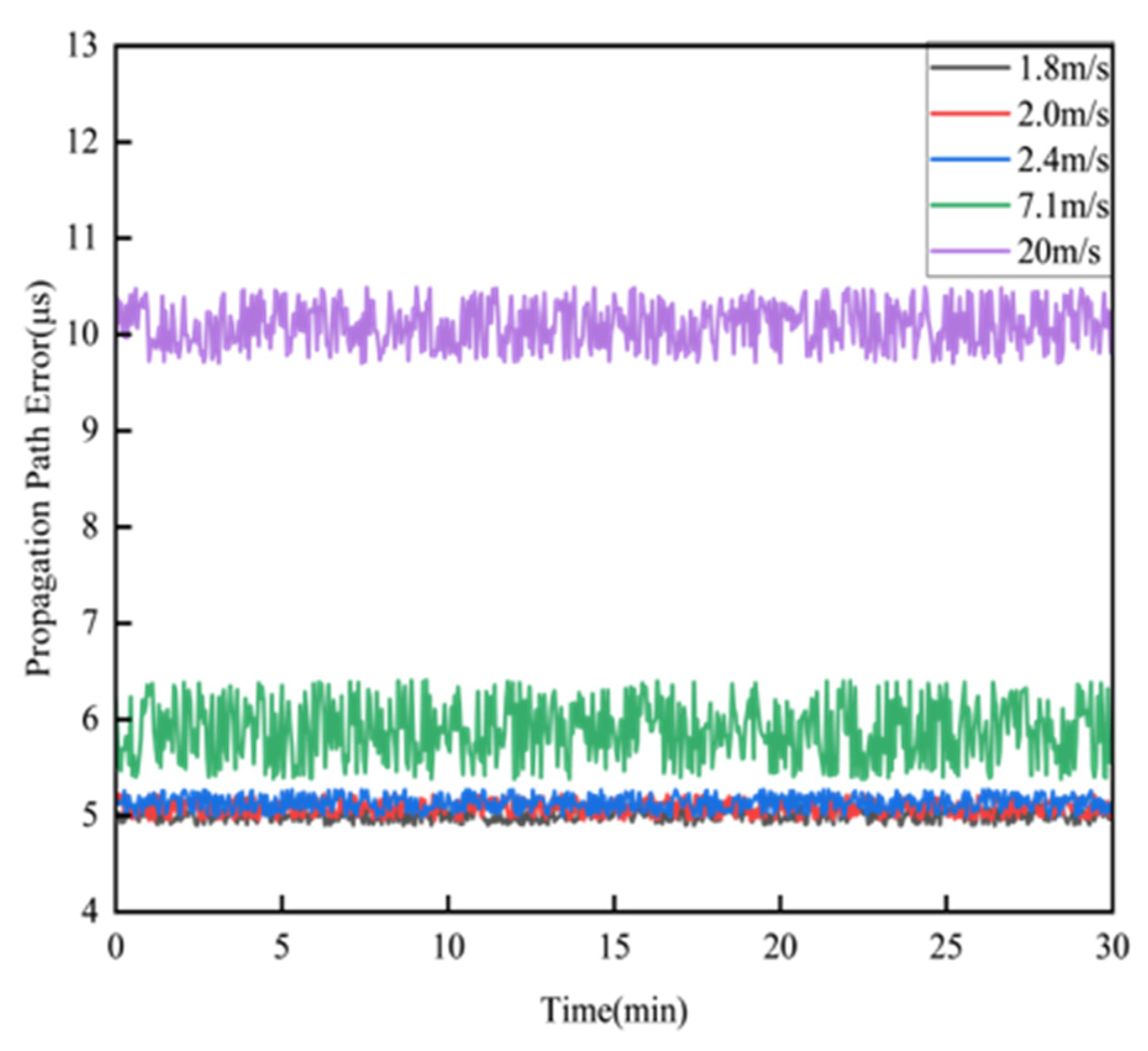
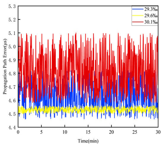
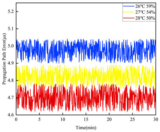
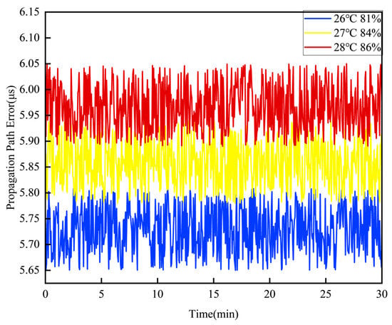
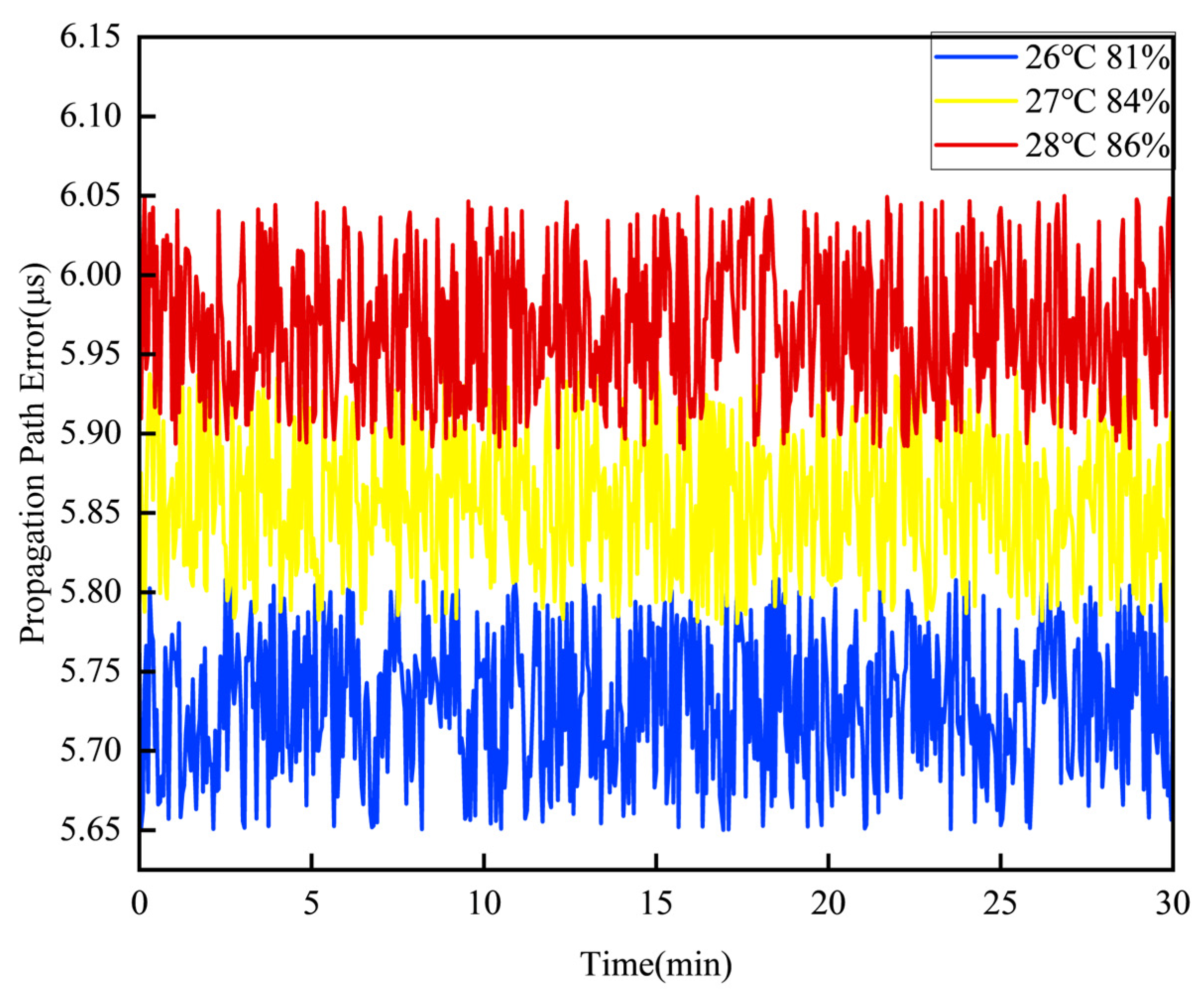
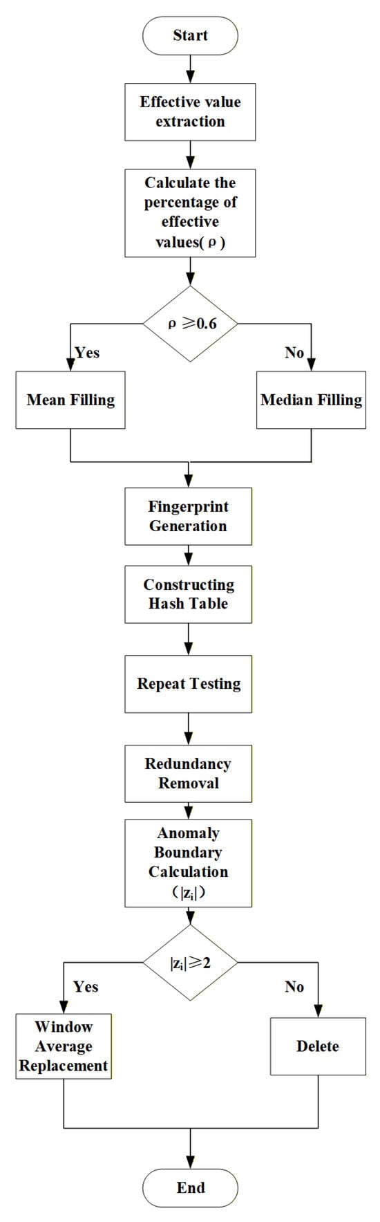
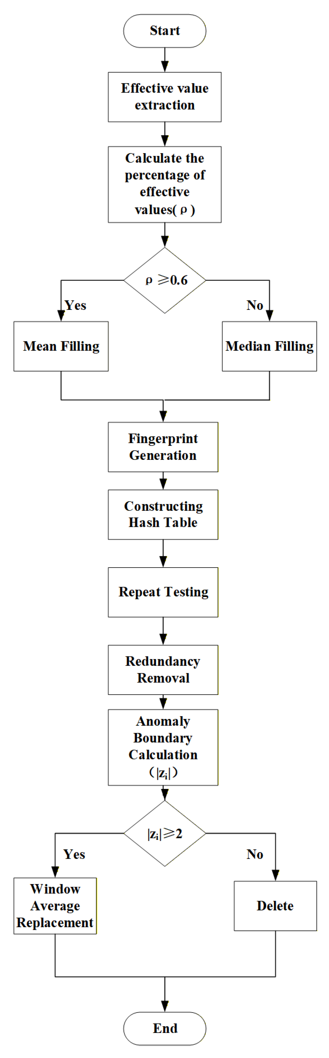
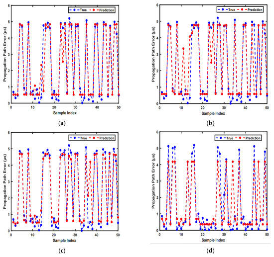
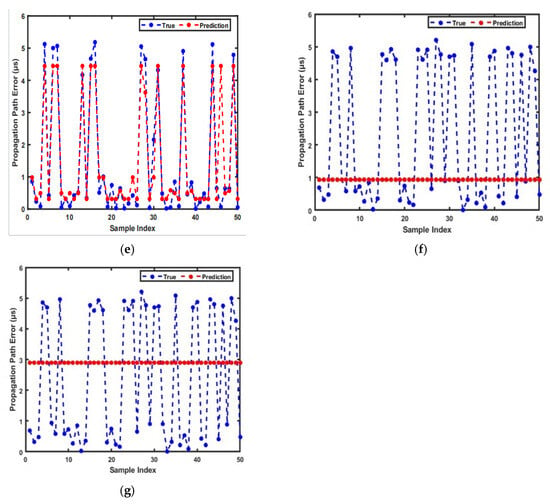
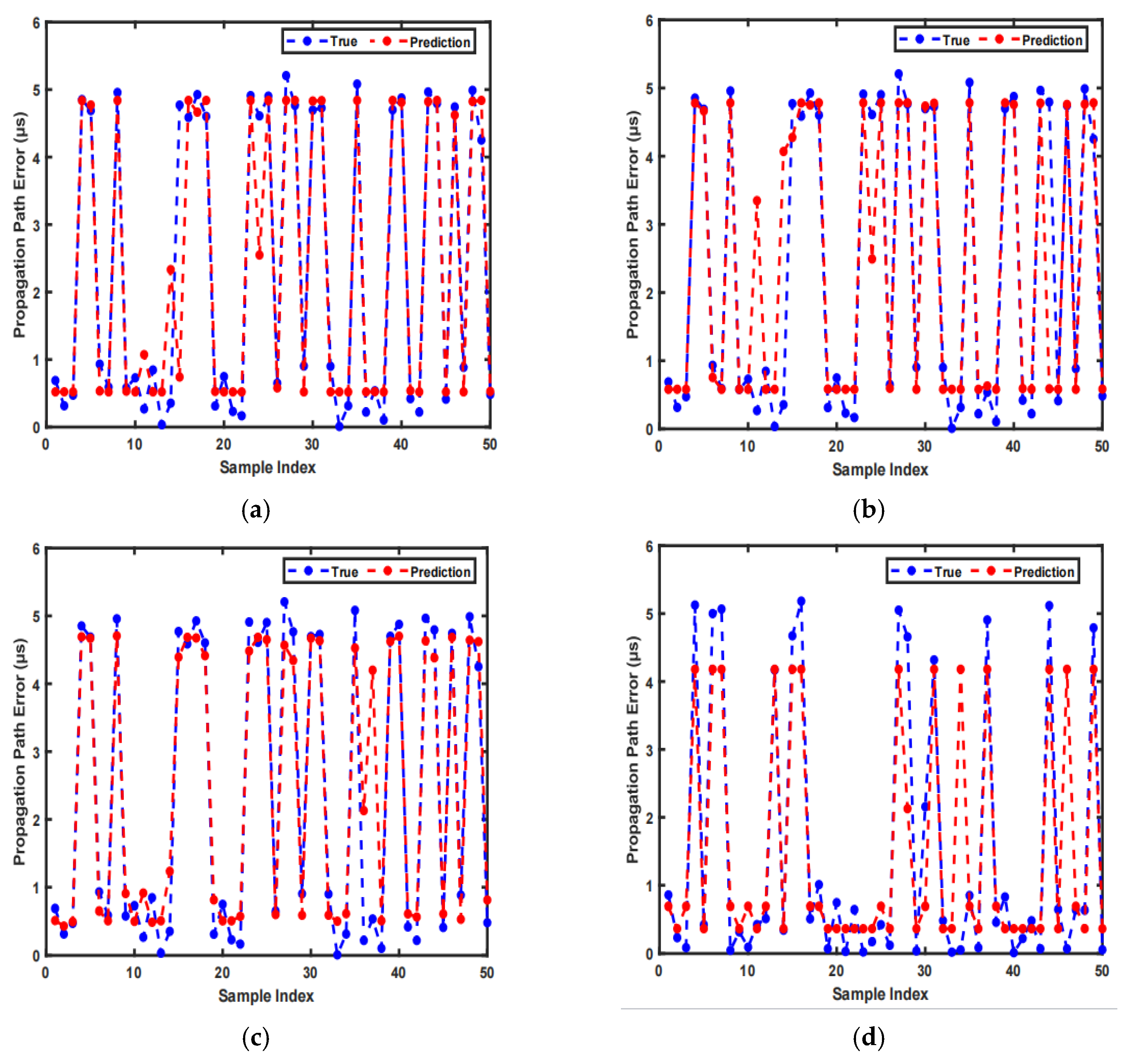
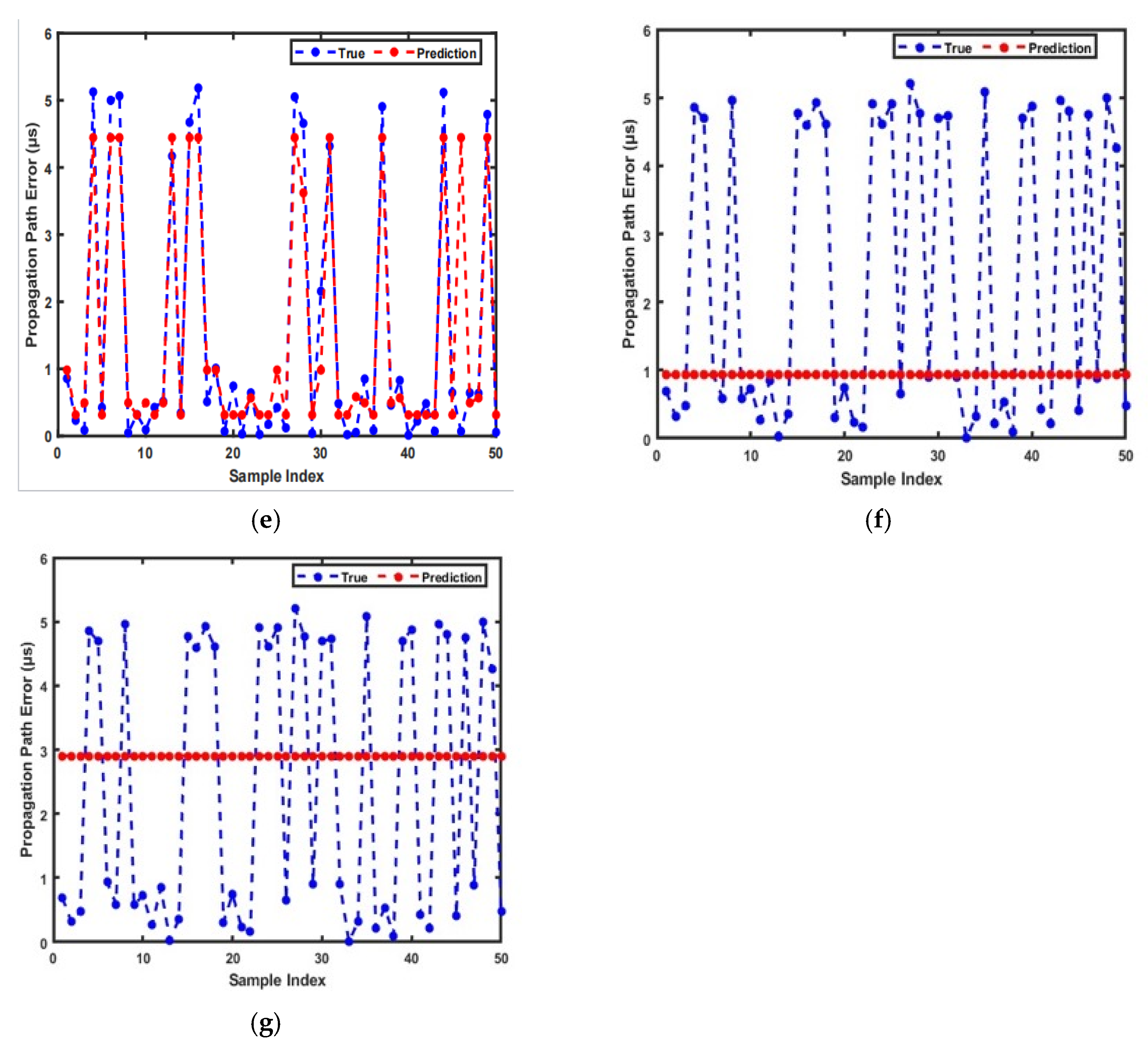

Disclaimer/Publisher’s Note: The statements, opinions and data contained in all publications are solely those of the individual author(s) and contributor(s) and not of MDPI and/or the editor(s). MDPI and/or the editor(s) disclaim responsibility for any injury to people or property resulting from any ideas, methods, instructions or products referred to in the content. |
© 2026 by the authors. Licensee MDPI, Basel, Switzerland. This article is an open access article distributed under the terms and conditions of the Creative Commons Attribution (CC BY) license.