


Abstract
Harmonic pollution may pose serious safety risks to power systems. Owing to its simplicity and ease of implementation, the fast Fourier transform (FFT) is one of the most widely used methods for harmonic analysis. However, its performance is limited by spectral leakage and the picket-fence effect caused by asynchronous sampling. Windowed interpolation techniques are commonly used to mitigate these effects. Although conventional window functions and interpolation methods have already demonstrated their effectiveness in harmonic detection, further improvements in parameter estimation accuracy remain desirable. Building on these approaches, this paper investigates a normalized multi-spectral-line weight calibration method based on the maximum sidelobe decay (MSD) dual-window all-phase spectrum. Within an existing framework combining multi-spectral-line interpolation and offline particle swarm optimization (PSO), the proposed method employs an MSD self-convolution all-phase spectrum. Nonnegativity and sum-to-one constraints are imposed on the weights assigned to the central, next-nearest, and outer spectral-line groups. The mean relative amplitude error is used directly as the fitness function for optimization, while frequency error serves as an independent evaluation metric after the optimized weights have been fixed. This formulation explicitly separates the objective used for weight calibration from the subsequent assessment of frequency estimation performance. The method addresses the limitations of traditional approaches that rely on empirical choices of spectral-line counts and weights, thereby further improving amplitude and frequency estimation accuracy. Simulation studies are conducted to verify the effectiveness of the proposed method for complex signals containing harmonic and interharmonic components. The results demonstrate that the method effectively reduces amplitude, frequency, and phase estimation errors for these components. Furthermore, it maintains favorable parameter estimation accuracy under fundamental-frequency fluctuations and white-noise interference, indicating its potential for harmonic analysis and power quality monitoring in power systems.
1. Introduction
In recent years, power grids have undergone rapid modernization and become increasingly intelligent. The widespread adoption of new electronic devices has made harmonic pollution in power systems increasingly prominent [1,2,3]. Harmonics cause voltage and current waveform distortion, increase additional equipment losses and temperature rise, and consequently degrade power quality and compromise the operational safety of power systems [4]. Therefore, accurate and rapid detection of harmonic content in power grids provides an effective basis for harmonic mitigation, thereby ensuring the safe operation of power systems.
Various methods have been investigated for harmonic analysis and related power-system signal estimation, including the fast Fourier transform (FFT) [5], wavelet transform [6,7], neural-network-based analysis [8,9], the Prony algorithm [10], the ip–iq method [11], and the matrix pencil method [12]. Among these, windowed interpolated FFT is one of the most widely used approaches. Its high computational speed and ease of implementation on embedded platforms make it well suited to practical applications. However, fully synchronous sampling is difficult to achieve in actual power grids because the frequency fluctuates continuously and the signal conditions are not always stable. Consequently, asynchronous sampling is commonly employed in signal acquisition. Under nonsynchronous sampling conditions, FFT-based analysis is affected by spectral leakage and the picket-fence effect, which introduce errors into harmonic parameter estimates [13].
Interpolated discrete Fourier transform (IpDFT) methods have a well-established foundation in signal parameter estimation. Grandke [14] developed interpolation algorithms for the DFT of weighted signals, while Andria et al. [15] investigated windowing and interpolation for accurate electrical measurements. Agrež [16] developed weighted multipoint DFT interpolation to improve the amplitude estimation of multifrequency signals.
To address these limitations, researchers have employed window functions with different spectral characteristics and spectral-line interpolation techniques to correct estimation errors. Several studies have proposed improved windowing and interpolation algorithms to enhance detection accuracy. To improve phase estimation accuracy, the all-phase fast Fourier transform (apFFT) has also been introduced. This method offers advantages in suppressing spectral leakage, while its phase invariance enables accurate phase estimation [17,18]. For example, Ref. [19] combines a Nuttall dual-window all-phase spectrum with four-spectral-line interpolation for harmonic parameter estimation.
Window function characteristics play a crucial role in suppressing spectral leakage [20]. Commonly used cosine-sum windows include the Hamming, Hann, flat-top, Blackman–Harris, Nuttall windows [21]. To further improve window performance, previous studies have proposed hybrid convolution windows of various orders and modified convolution window structures. Reference [22] investigated an interpolated FFT method based on a hybrid convolution window. Reference [23] analyzed the effects of convolution order on sidelobe attenuation and mainlobe width. Reference [24] proposed a structure obtained by convolving Slepian and Parzen windows and evaluated its performance in harmonic analysis. These studies demonstrate that hybrid convolution can improve sidelobe suppression but may also produce an excessively wide mainlobe. Therefore, window selection requires a balance between sidelobe attenuation and frequency resolution.
Improved sidelobe suppression often comes at the expense of a wider mainlobe. In addition, spectral-line interpolation is used to reduce parameter-estimation errors associated with discrete spectral sampling. Conventional multi-spectral-line interpolation methods typically employ predefined decreasing weights based on the distance of each spectral line from the spectral peak and the spectral characteristics of the window. Such fixed weights, however, are not necessarily suitable for different window functions and signal conditions. Common approaches include four-spectral-line interpolation [25] and six-spectral-line interpolation [26,27]. In Doppler signal processing, Ref. [28] employed a hybrid convolution window combining a four-term Nuttall window and a five-term Rife–Vincent window, together with fixed weights for six-spectral-line interpolation. Reference [29] further adopted a hybrid convolution structure combining a Blackman–Harris window and a five-term MSD window. Based on the conventional FFT, particle swarm optimization was used to optimize the six-spectral-line weights, while polynomial fitting was employed to correct frequency deviation and amplitude estimates. However, a sum-to-one normalization constraint was not imposed on the spectral-line weights in Ref. [29].
Reference [19] employs a Nuttall dual-window all-phase FFT with fixed four-line interpolation, whereas Ref. [29] investigates offline PSO-based spectral-line weight optimization using a Blackman–Harris/MSD hybrid convolution window. The present work extends these approaches by developing a normalized multi-line interpolation calibration specifically for the MSD self-convolution all-phase spectrum. Compared with Ref. [19], the proposed formulation introduces a six-line candidate structure with calibrated relative weights instead of a fixed four-line configuration. Compared with Ref. [29], the interpolation model and its correction functions are formulated for the MSD self-convolution all-phase response, rather than the hybrid convolution-window spectrum.
The contribution lies in the consistent calibration of the spectral-line weights, inverse frequency-offset mapping, and amplitude-correction function for this spectral response. For each candidate weight vector, the correction functions are refitted before the estimation error is evaluated. Nonnegative, sum-to-one constraints remove the redundant overall weight scale and allow individual spectral-line pairs to receive zero weight, enabling the calibration to determine an effective combination within the candidate structure. PSO is employed as the offline numerical solver for this calibration. Subsequent simulations evaluate the estimation performance under harmonic and interharmonic conditions, white-noise interference, and fundamental-frequency variations.
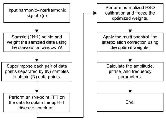
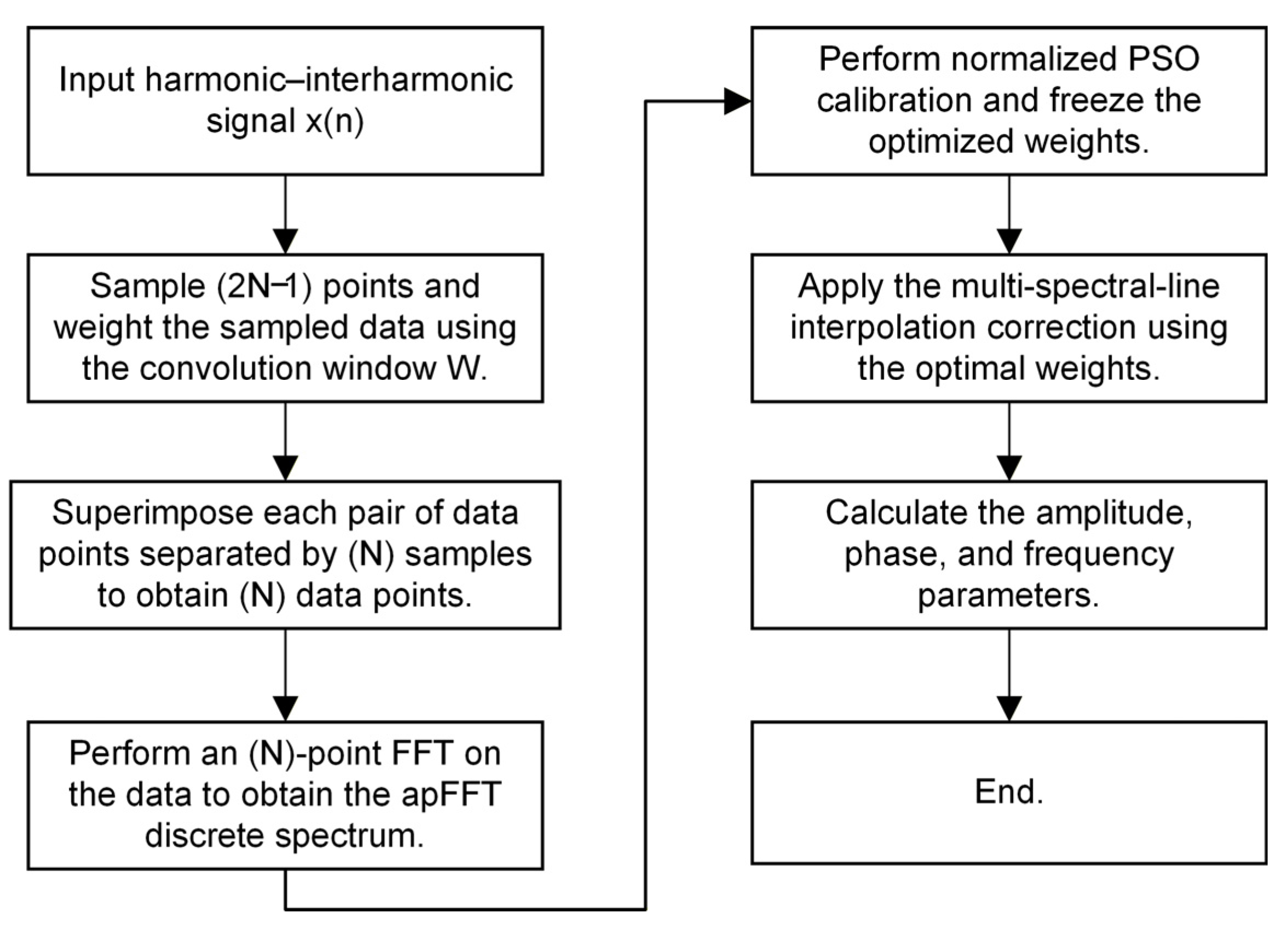
The overall procedure of the proposed algorithm is illustrated in the following Figure 1.
Figure 1.
The principle of algorithm flowchart.
2. Dual-Window All-Phase Analysis
2.1. Selection of the Window Function
Classical cosine-sum windows are widely used, and their time-domain expression is given by:
where M is the number of terms in the window function, am denotes the window coefficients, and n = 0, 1, 2, …, N−1. The following constraints must also be satisfied:
Window function selection primarily aims to achieve a narrow mainlobe and favorable sidelobe characteristics. A narrower mainlobe provides higher frequency resolution, while a lower peak sidelobe level and a faster sidelobe decay rate concentrate more signal energy within the mainlobe, thereby improving spectral leakage suppression. Since these objectives generally involve a trade-off, window selection should balance both characteristics, favoring superior sidelobe performance while meeting the resolution requirements for closely spaced frequency components.
In this study, window functions are selected for the analysis of signals containing harmonics up to the 21st order and complex interharmonic components. The table presents a comparison of the performance characteristics of different window functions.
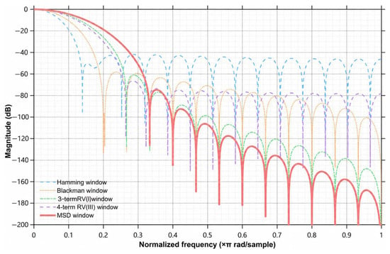
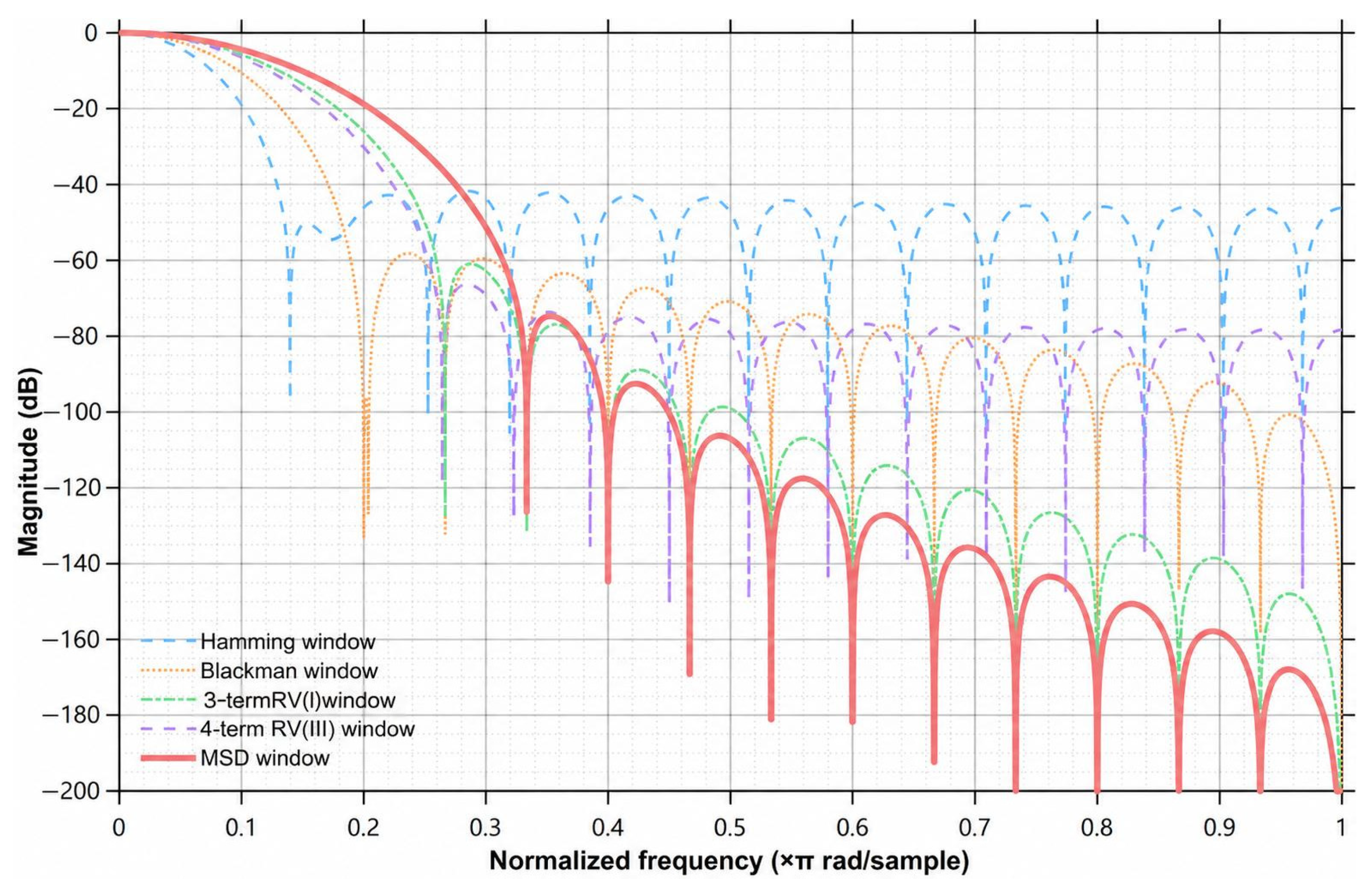
As shown in Table 1 and Figure 2, the five-term MSD window exhibits a lower peak sidelobe level and a faster asymptotic sidelobe decay rate. Combining this window with all-phase processing helps suppress spectral leakage between adjacent mainlobes and attenuate distant sidelobes. The coefficients of the five-term MSD window are as follows: a0 = 0.2734375, a1 = 0.4375000, a2 = 0.2187500, a3 = 0.0625000, and a4 = 0.0078125.
Table 1.
Common Characteristics Indexes of Window Functions.
Figure 2.
Comparison of the normalized magnitude spectra of the selected window functions.
2.2. Principles of the All-Phase FFT
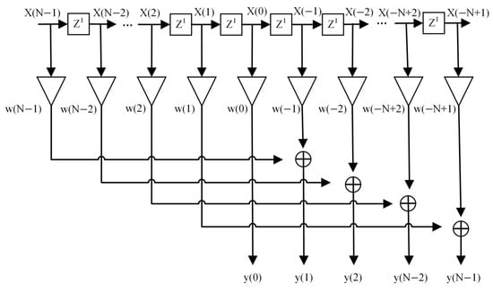
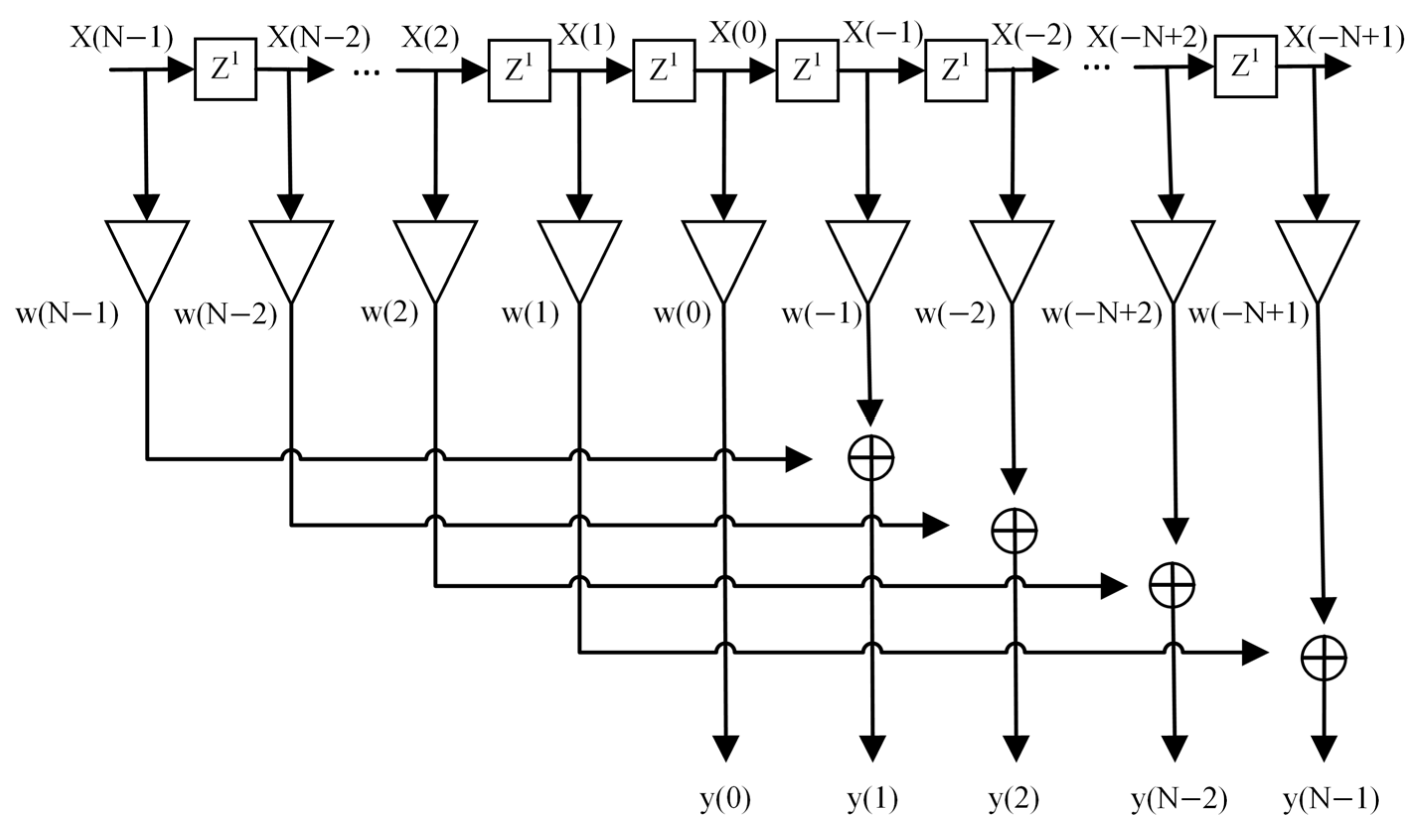
As illustrated in Figure 3, preprocessing in the apFFT method proposed in the literature involves segmenting the signal, cyclically rearranging the segments, and summing them to obtain an all-phase periodically extended signal. The procedure is described below.
Figure 3.
Flowchart of all-phase data preprocessing.
Consider an original signal consisting of 2N−1 samples. By sliding a window of length N over the signal, N overlapping subsequences are obtained. The first subsequence, x0, contains samples indexed from 0 to N−1; the second subsequence, x1, contains samples indexed from 1 to N; and so forth. The final subsequence, xN−1, contains samples indexed from N−1 to 2N−2.
Using the central sample of the original sequence as the reference point, each subsequence is cyclically rearranged by moving the samples preceding the reference point to the end while preserving their order. The N rearranged subsequences are then summed to form the all-phase periodically extended signal. Finally, an FFT is applied to obtain the apFFT result.
The detailed data processing procedure is shown in Figure 3.
The convolution window ωc(n) is obtained by convolving the front window ω1 with its time-reversed counterpart, the rear window ω2:
Since the rear window is the time-reversed version of the real-valued front window, the spectrum of the convolution window is given by:
where |W1(ω)|2 denotes the squared magnitude of the window function’s frequency response.
2.3. Spectral Analysis of the MSD Dual-Window All-Phase Method
To analyze the performance of the proposed algorithm and clarify the computational procedure, a single-frequency sinusoidal signal is first considered to examine the spectral characteristics of the dual-window all-phase method:
where A is the amplitude, f0 is the frequency, φ0 is the initial phase, and fs is the sampling frequency. Based on the all-phase processing principle and the symmetry of the convolution window, the data obtained after weighted pairwise summation can be expressed as:
where n = 0, 1, 2, …, N − 1.
The unnormalized N-point DFT of the folded sequence is given by:
The discrete spectrum near the positive-frequency component f0 can be expressed as:
Compared with the conventional FFT, the apFFT reduces the influence of shifts in the signal starting point on the spectral phase. For the sinusoidal signal model adopted in this study, a reference phase compensation of +π/2 is applied to the phase of the left spectral line k3 in the selected central pair and the final phase estimate is obtained through phase wrapping. Phase estimation is not involved in the PSO-based weight optimization. Furthermore, in all-phase FFT analysis, the sidelobes of the MSD self-convolution window decay more rapidly with increasing distance from the mainlobe, concentrating more spectral energy near the mainlobe. This effectively suppresses spectral leakage and improves detection accuracy.
3. Particle Swarm Optimization-Based Interpolation Algorithm
3.1. Principles of Multi-Spectral-Line Interpolation
Although windowing effectively suppresses spectral leakage, the picket-fence effect remains a source of estimation errors in harmonic detection. Spectral-line interpolation algorithms are commonly employed to correct harmonic parameter estimates and reduce these errors. Fixed-weight multi-spectral-line interpolation methods combine neighboring spectral magnitudes using predefined weighting coefficients [25,26,27]. Although these coefficients are selected for particular window responses and interpolation formulas, they are not necessarily optimal for the MSD dual-window all-phase spectrum and calibration objective considered here.
The first spectral nulls of the MSD dual-window all-phase spectrum are located five FFT bins on either side of the peak, corresponding to a null-to-null mainlobe width of 20π/N. The number of spectral lines should be selected such that their distances from the true frequency remain within the mainlobe. For the six-line configuration, the maximum distance between any selected spectral line and the true frequency does not exceed three FFT bins. Thus, all six lines lie within the mainlobe and satisfy this requirement. The six selected lines form a candidate interpolation structure with three symmetric weight groups corresponding to the outer, intermediate, and central pairs. Nonnegative weights are assigned subject to a + b + c = 1. This formulation permits individual pairs to receive zero weight, allowing the calibration to determine which groups contribute to the final weighted estimator. Thus, the six-line model does not require all six lines to have nonzero contributions. The candidate range is restricted to these six positions because lines farther from the peak approach the first spectral nulls, where the target-component contribution decreases and interference from noise or neighboring components may become more influential.
Therefore, this study adopts a six-spectral-line interpolation framework and defines the corresponding parameters. The amplitude information from spectral lines near the mainlobe is used to reconstruct the target spectral peak, determine the optimal weights, and substitute them into the interpolation equations for parameter estimation.
Let the sampling frequency be fs and the FFT length be N. The DFT-bin spacing is then given by:
For the harmonic component to be estimated, six consecutive spectral lines in its vicinity are selected, with indices denoted by k1, k2, k3, k4, k5, and k6, where k3 is the index of the left spectral line in the detected central pair. The continuous-valued frequency-bin coordinate corresponding to the midpoint of the six spectral lines is defined as:
Let the true signal frequency be f0 and its normalized frequency-bin position be . The normalized frequency offset is then defined as:
Therefore, the true frequency can be expressed as:
In this study, the six spectral lines are assigned symmetric weights a, b, c, c, b, a, where a, b, and c denote the weights of the outer, intermediate, and central spectral-line pairs, respectively. A six-spectral-line relation, β, is formulated to determine the frequency offset α. Let:
Define as the dual-window frequency response expressed in units of DFT-bin spacing. Let
Thus, we obtain:
For each fixed weight combination, Equations (15)–(17) establish the relationship between the normalized frequency offset α and the spectral statistic β. The inverse relationship is approximated by the seventh-degree odd polynomial pf (β) in Equation (18). Its coefficients are obtained by least-squares fitting using the basis {β, β3, β5, β7}, with β as the input and the true calibration offset α as the target.
Here, d1, d3, d5, and d7 are the fitted polynomial coefficients.
From the above, the frequency fh of the h-th harmonic can be obtained as:
Using the weighted sum of the six spectral-line magnitudes, the amplitude relationship is obtained as:
Define the scaled amplitude-correction function as:
The amplitude correction is implemented using a sixth-degree even polynomial h. After fitting pf, the estimated offsets are used as inputs to fit h, with AiN2/Ti as the targets, where Ti is the weighted spectral-line sum for calibration sample i. The resulting amplitude estimator is given by Equation (22).
Since the algorithm proposed in this paper employs the apFFT, its phase-invariance property significantly reduces the sensitivity of spectral-line phase estimation to shifts in the starting point. In the program, a reference phase compensation term, π/2, is added to the phase of the left spectral line k3 in the selected central pair, and the final phase estimate is obtained through phase wrapping, such as
3.2. Weighted-Coefficient Evaluation Function
Based on the above conclusions, only the corrected amplitude and frequency results are closely related to the values of {a,b,c}. By applying first-order error propagation to the frequency and amplitude, respectively, we obtain
Further eliminating , we obtain
The frequency error is mainly propagated through the frequency-offset mapping function, whereas the amplitude error is affected by both the variation in the total spectral-line magnitude and the frequency-offset estimation error. Therefore, the frequency and amplitude errors exhibit a coupled dependence on the weighting parameters. Consequently, the weights optimized with respect to the amplitude objective can still maintain a relatively small frequency estimation error.
A common positive scaling of all three weights leaves the frequency-offset statistic β unchanged. Therefore, the constraints a + b + c = 1 and a, b, c ≥ 0 are imposed to remove the redundant overall scale and express the calibration directly in terms of the relative contributions of the outer, intermediate, and central spectral-line pairs. Normalization itself does not improve estimation accuracy when the relative weights remain unchanged.
The weights determine both the frequency-offset statistic and the weighted spectral magnitude used for amplitude estimation. Consequently, each candidate weight vector must be evaluated together with its associated correction functions. In the calibration procedure, the inverse frequency-offset mapping and amplitude-correction function are refitted on the training set for every candidate weight vector. The resulting amplitude and frequency errors are then evaluated on the validation set to calculate the selected objective in Equations (27)–(29). For the final amplitude-only method, only the amplitude objective is minimized.
This procedure ensures that the selected weights and correction functions are matched to the same MSD self-convolution all-phase spectrum.
To investigate the effects of different optimization objectives on the measurement accuracy, for the i-th calibration sample, let the amplitude and frequency estimates obtained using the six-spectral-line weighted model be denoted by and , respectively. The amplitude-only objective function, frequency objective function, and joint objective function are defined as follows:
where M denotes the number of samples in the validation set; Ai and fi denote the true amplitude and true frequency of the i-th sample, respectively; Âi and denote the corresponding estimated values; and ε is a numerical stabilization term introduced to prevent denominator degeneration.
Here, and are fixed positive normalization constants obtained by evaluating a common reference weight vector on the validation set after fitting its correction functions on the training set. The coefficient λA controls the contribution of the amplitude objective: λA = 1 corresponds to amplitude-only optimization, λA = 0 corresponds to frequency-only optimization, and 0 < λA < 1 gives a joint objective. The frequency metric Jf in Equation (28) is the frequency RMSE in Hz, rather than the mean relative frequency error.
For this comparison, the reference weights are (aref, bref, cref) = (0.123716409456439, 0.031070035510314, 0.845213555033247), corresponding to the outer, intermediate, and central spectral-line pairs, respectively. The resulting normalization constants are 4.3823514683 × 10⁻¹¹ and 1.2534360267 × 10⁻⁹ Hz.
In this paper, the final optimization objective is selected by comparing the results of the single-objective and joint-objective experiments.
3.3. Principle of the Particle Swarm Optimization Algorithm
The particle swarm optimization (PSO) algorithm is inspired by the foraging behavior of bird flocks, in which all possible solutions are abstracted as individual particles. As the particles move through the search space, their positions are dynamically updated by tracking two target positions: the personal best position and the global best position. Each particle is characterized by two attributes, namely velocity and position, which represent its moving direction and speed, and its current candidate solution in the search space, respectively. In this way, the particles search for the optimal solution efficiently. By integrating individual experience with collective intelligence, the particle swarm can effectively explore complex search spaces and converge toward the optimal solution.
Consider a swarm of n particles in a D-dimensional search space. At iteration k, let xiᵏ and viᵏ denote the position and velocity vectors of particle i, respectively. Let piᵏ denote the best position found by particle i up to iteration k, and let gᵏ denote the best position found by the swarm up to that iteration. For i = 1, …, n and d = 1, …, D, the velocity and position are updated as follows:
Here, ω is the inertia weight; c1 and c2 are the cognitive and social acceleration coefficients, respectively; r1 and r2 are uniformly distributed random numbers in [0,1]; and Δt is the update time step, set to 1 in this study.
To prevent particles from moving outside the search space, boundary constraints are imposed. The upper and lower velocity limits are set to vmax and vmin, respectively, while the position is constrained within [xmin,xmax]. In this study, the PSO algorithm employs 36 particles and 150 iterations. The inertia weight is set to 0.78, both the cognitive and social learning factors are set to 1.6, and the velocity range is [−0.25,0.25]. A two-dimensional parameterization is adopted in the PSO algorithm to generate weight vectors satisfying the above constraints, such that only the relative weighting relationships among the spectral lines are optimized.
PSO is selected as the offline solver because each objective evaluation involves refitting the frequency-offset and amplitude-correction functions and calculating the resulting estimation error. It can directly use this numerical evaluation procedure without requiring derivatives of the objective function. Its population-based updates adjust candidate positions in the continuous feasible space using individual and collective search information. This provides a practical means of searching for suitable relative spectral-line weights without prescribing a fixed discretization of the feasible domain. After calibration, the weights and polynomial coefficients remain fixed, and no PSO iterations are required during online parameter estimation.
3.4. PSO-Based Multi-Spectral-Line Interpolation Weight Optimization
To avoid using the same data for both weight optimization and performance evaluation, the single-component calibration samples are divided into a training set, a validation set, and an independent test set, containing 600, 300, and 600 samples, respectively. The corresponding random seeds are set to 511, 512, and 513. Noise-free signals are used during the calibration stage. A single-component calibration dataset is constructed under the conditions of =5120 Hz and N = 2048, resulting in a frequency resolution of =2.5 Hz. For each sample, the integer spectral-line index k is randomly selected within 30 < k < 994, and the normalized frequency offset is uniformly generated within . The signal frequency is then calculated according to Equation (13). The signal amplitude is generated from a log-uniform distribution over the range [0.05,2.0], while the initial phase is uniformly distributed over [0,2π].
During the iterative optimization process, the training set is used to fit the inverse frequency-offset mapping function and the amplitude correction function, whereas the validation set is used to compare candidate weight combinations and select the optimal solution. The correction functions are subsequently refitted using the training and validation sets, while the independent test set is used exclusively for the final performance evaluation.
To compare the effects of different optimization objectives, five values of λA, namely 1, 0.75, 0.50, 0.25, and 0, are evaluated under the same configuration of fs = 5120 Hz and N = 2048. All cases use the same training, validation, and independent test sets containing 600, 300, and 600 samples, respectively. For each value of λA, PSO is executed with 10 random seeds, and the candidate with the lowest corresponding validation objective is selected. The correction functions are then refitted using the combined training and validation sets before evaluation on the independent test set. The test set is not used to select the weights.
To select a compromise across the evaluated coefficients, the comparison score is defined as R = max(JA/A0, Jf/F0), where A0 = 2.4990033700 × 10⁻¹¹ and F0 = 5.9498080657 × 10⁻¹⁰ Hz are the lowest amplitude and frequency objectives found in the corresponding single-objective validation searches. These reference values are distinct from the normalization constants in Equation (29). The smallest R among the evaluated joint settings is obtained at λA = 0.0036666667. This is a selected numerical compromise, rather than a proven global optimum. After selection, the weights are fixed and the correction functions are refitted on the combined training and validation sets before independent testing. The test set is not used to select the weights or the mixing coefficient. Table 2 shows the relevant parameters.
Table 2.
Validation amplitude errors for different calibration objectives.
The amplitude metric is dimensionless, whereas the frequency RMSE is expressed in Hz. All errors are evaluated on the same independent test set after refitting the correction functions using the combined training and validation sets.
On the original 600-sample test set, frequency-only calibration reduces frequency RMSE by approximately 38.92% relative to the retained amplitude-only method, but increases the mean relative amplitude error to approximately 304 times its value. The joint settings λA = 0.75, 0.50 and 0.25 remain close to the amplitude-only solution, with reductions in test amplitude error below 0.02% and in frequency RMSE below 0.003%. The validation-selected compromise at λA = 0.0036666667 explores a different trade-off: its test frequency RMSE decreases from 9.5440723 × 10⁻¹⁰ Hz to 9.5149776 × 10⁻¹⁰ Hz, approximately 0.30485%, whereas its mean relative amplitude error increases from 2.499004 × 10⁻¹¹ to 4.0237798 × 10⁻¹¹. Thus, the selected compromise does not improve both test metrics relative to amplitude-only calibration.
Because this study prioritizes amplitude estimation accuracy, amplitude-only calibration is retained for the final method. It avoids the additional choice of a mixing coefficient while providing frequency accuracy close to that of the tested joint settings. Frequency RMSE is reported as an independent evaluation metric for the final amplitude-only method.
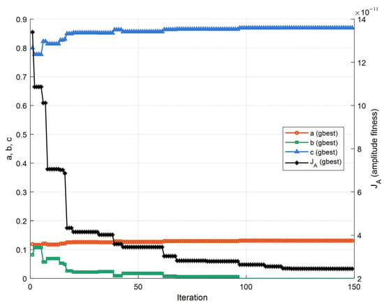
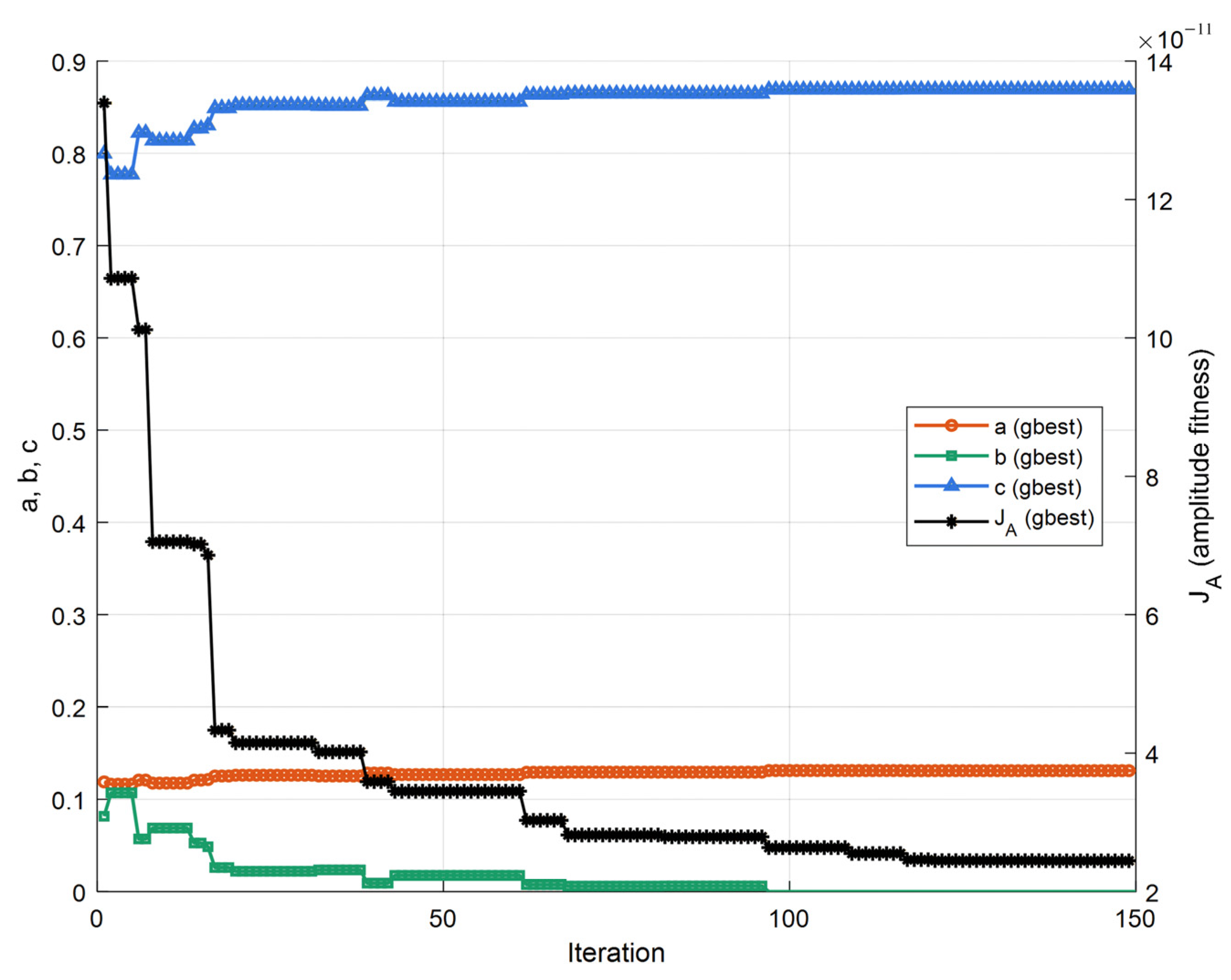
To assess the sensitivity to random initialization, PSO is independently executed using 10 different random seeds. During each run, the correction functions are fitted on the training set for every candidate weight vector, and the mean relative amplitude error on the validation set is used as the fitness value. The candidate with the lowest validation error across the 10 runs is selected. Once the weights are fixed, the correction functions are refitted using the combined training and validation sets, while the independent test set is reserved for the final evaluation. Convergence of normalized six-line weights and amplitude fitness during PSO show in Figure 4.
Figure 4.
Convergence of normalized six-line weights and amplitude fitness during PSO.
As can be seen from the figure, the major adjustment of the weighting parameters is completed within the first 30 iterations. Thereafter, the fitness function gradually approaches a stable value, and the subsequent iterations only make minor refinements to the weights. After 150 iterations, the normalized weights are obtained as a* = 0.130962417, b* = 0, and c* = 0.869037583. The corresponding amplitude fitness value on the validation set is = 2.499004 × 10⁻¹¹. After the optimization is completed, the continuous-valued weight results are retained and used for the subsequent polynomial fitting and performance testing.
Supplementary transfer tests retained the calibrated weights and correction coefficients while updating the window length and the corresponding frequency and amplitude scaling. Across the five tested configurations, fs = 5120 Hz with N = 1024, 2048 and 4096, and N = 2048 with fs = 4096 and 8192 Hz, the mean relative amplitude error remained between 2.39 × 10⁻¹¹ and 2.55 × 10⁻¹¹ for independent noise-free single tones at 150–1800 Hz. Refitting the correction functions with fixed weights produced negligible changes. These results support reuse of the calibration within the tested conditions, without establishing optimality or validity for arbitrary configurations, noise distributions or interfering components.
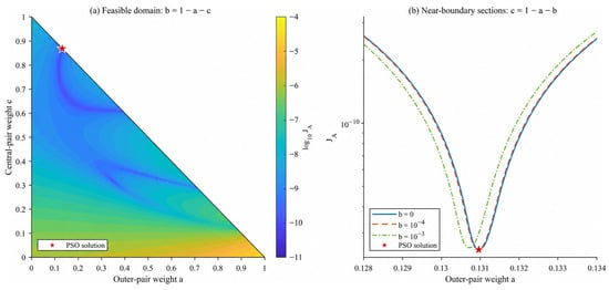
To further examine the calibrated weights, the objective landscape is evaluated over the feasible domain a ≥ 0, c ≥ 0, and a + c ≤ 1, with b = 1 − a − c. For each evaluated weight vector, the correction functions are refitted on the training set, and JA is calculated on the validation set. The contour plot of log10JA and the near-boundary sections illustrate the variation in the calibration objective around the reported PSO solution, providing complementary information to the convergence curve.
The selected solution lies on the boundary b = 0, which is permitted by the nonnegative constraints. The intermediate pair therefore receives zero weight, while the central and outer pairs contribute to the weighted interpolation. Nine of the ten recorded PSO runs also returned b = 0. This result indicates that a positive contribution from every candidate line is not required under the investigated calibration conditions. The six-line structure is therefore interpreted as a candidate model with four nonzero line weights in the selected solution. This observation does not imply that the same configuration is optimal for other windows, noise levels, or signal conditions. Objective landscape of the normalized spectral-line weight calibration shows in Figure 5.
Figure 5.
Objective landscape of the normalized spectral-line weight calibration.
(a) Contours of log10J A over the feasible (a, c) domain, with b = 1 − a − c; the star marks the PSO solution. (b) Near-boundary objective sections for b = 0, 10−4, and 10−3, with c = 1 − a − b. The correction functions are refitted for every evaluated weight vector using the same calibration data.
With the optimized weights fixed, the frequency-offset polynomial pf(β) and the amplitude-correction polynomial are refitted using the combined training and validation sets. The frequency-offset polynomial contains odd powers up to degree seven, whereas the amplitude-correction polynomial contains even powers up to degree six. The fitted expressions are given below.
Substituting the optimized weights into Equation (14) and combining Equations (18), (19), and (22), the final amplitude and frequency estimators are expressed as follows:
Here, β is calculated from Equation (14) using the same optimized weights a*, b*, c*. Since b* = 0, the intermediate spectral lines y2 and y5 have zero weight in both the frequency-offset statistic and the amplitude estimator. The continuous-valued weights are retained without integer rounding.
For each target component, the spectral statistic β is first calculated using Equation (14), followed by the frequency-offset estimate in Equation (18). The frequency and amplitude are then estimated using Equation (32), while the phase is estimated separately using Equation (23).
Accordingly, the amplitude, frequency, and phase parameters of each component in the complex harmonic signal can be finally determined.
4. Simulation Analysis
4.1. Case Study of Integer Harmonic Signals
Based on the characteristics of practical power-grid signals, the complex harmonic signal model adopted in this study is expressed as
where h denotes the harmonic order, H is the highest harmonic order, and n denotes the discrete-time sample index. A test signal containing harmonic components up to the 21st order is generated in MATLAB2024a. The sampling frequency is 5120 Hz, the FFT length is N = 2048, and the fundamental frequency is 50.1 Hz. Methods 1 and 4 use 2048 raw samples, whereas Methods 2, 3, 5 and 6 use 4095 raw samples, corresponding to observation durations of approximately 0.4 s and 0.8 s, respectively. The signal parameters are listed in Table 3. The phase values in Table 3, Table 4 and Table 5 are reported in degrees and are converted to radians for signal generation and parameter estimation.
Table 3.
Parameters of the 21-component harmonic test signal.
Table 4.
Parameters of the nine-component interharmonic test signal.
Table 5.
Parameters of the combined harmonic and interharmonic test signal.
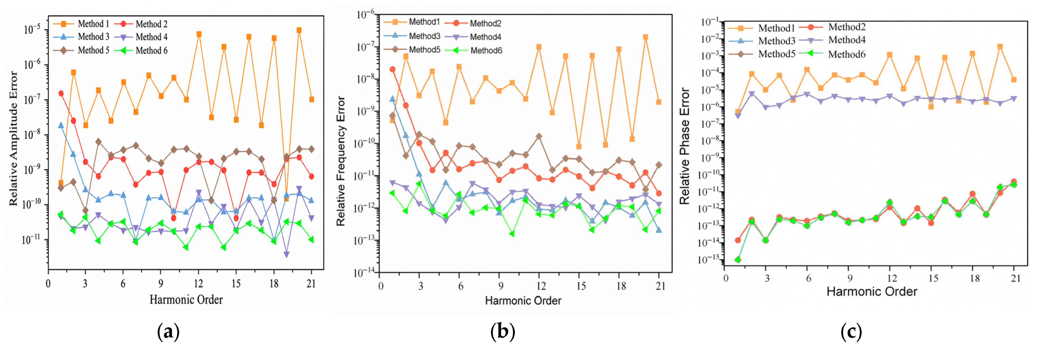
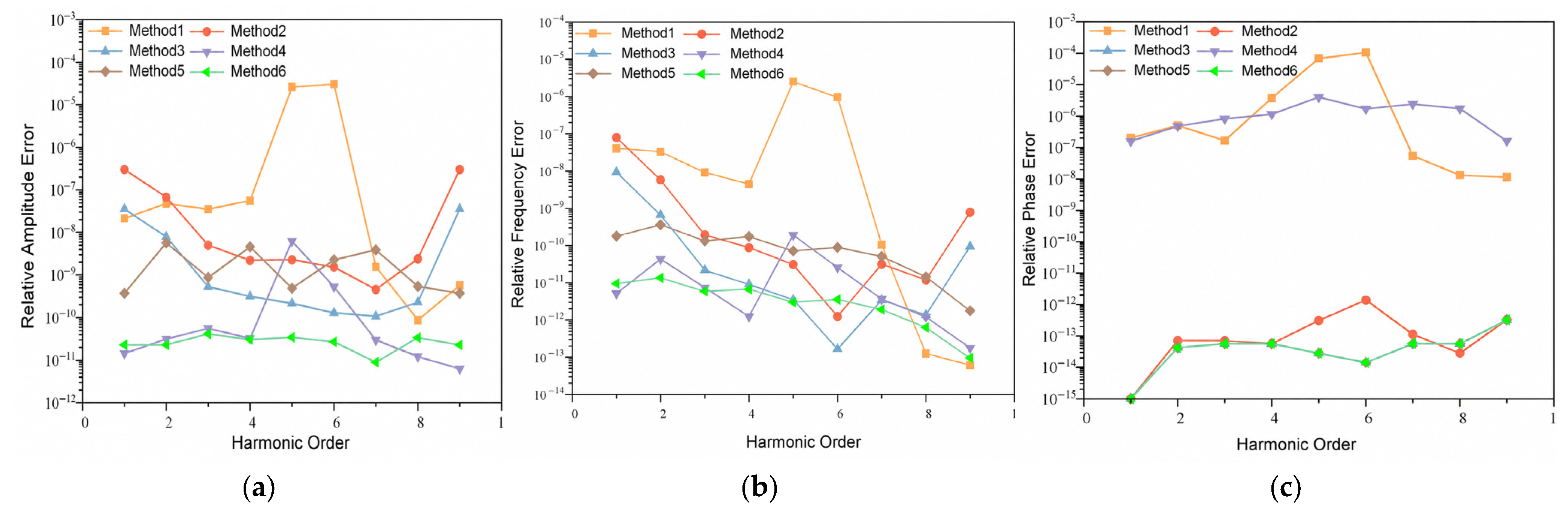
To evaluate the detection performance of the MSD dual-window all-phase method combined with the PSO-based spectral-line interpolation algorithm, six methods are compared using a common sampling frequency and FFT length, with the raw-record lengths specified above. The specific configurations are as follows: Method 1 is the MSD-window six-spectral-line interpolation algorithm (a = 1, b = 2, c = 6); Method 2 is the Nuttall dual-window apFFT four-spectral-line interpolation method reported in Ref. [19] (a = 1, b = 2); Method 3 is the MSD dual-window apFFT six-spectral-line interpolation algorithm (a = 1, b = 2, c = 6); Method 4 is the BH-M hybrid convolution-window PSO six-spectral-line interpolation algorithm reported in Ref. [29] (a = 7, b = 0, c = 8); Method 5 is the MSD dual-window apFFT PSO four-spectral-line interpolation algorithm (a = 0.605286, b = 0.394714); and Method 6 is the proposed MSD dual-window apFFT method with PSO-optimized spectral-line interpolation algorithm (a = 0.130962, b = 0, c = 0.869037). The relative errors in amplitude, frequency, and phase estimation obtained using the six methods are compared in Figure 6.
Figure 6.
Relative errors for 21 harmonics. (a) Relative amplitudes errors; (b) Relative frequency errors; (c) Relative phase Errors.
The difference in raw-record length arises from the all-phase preprocessing used in this study. The conventional windowed FFT methods process N raw samples, whereas the adopted dual-window all-phase methods preprocess 2N − 1 raw samples to form an N-point sequence for the FFT. Fixing the sampling frequency and FFT length therefore provides a common FFT-bin spacing while retaining the respective processing structures. This comparison characterizes the complete implementations rather than performance at an equal observation duration. Importantly, Methods 3 and 6 use the same raw-record length and all-phase preprocessing, so their performance difference is not caused by a longer observation record for Method 6.
According to the test results shown in Figure 6, under the condition of harmonics up to the 21st order, a comparison between the conventional Method 1 and the improved Method 6 proposed in this paper shows that, relative to the conventional FFT-based method without optimization, the proposed method achieves substantially higher accuracy for all measured components. In terms of amplitude, frequency, and phase estimation, the proposed algorithm exhibits superior measurement stability and accuracy.
Compared with Method 2, which employs the Nuttall dual-window all-phase FFT four-spectral-line interpolation algorithm reported in Ref. [19], Method 6 achieves higher accuracy in both amplitude and frequency estimation. The corresponding errors are reduced by approximately 99.71% and 99.76% on average, respectively. The phase accuracies of the two methods are relatively close. These results indicate that the MSD dual-window all-phase spectrum and the normalized multi-spectral-line weighting calibration model developed in this paper can effectively reduce deterministic interpolation bias under isolated-component conditions.
Compared with Method 3, the proposed Method 6 reduces the amplitude estimation error in the noise-free 21-harmonic test. The relative amplitude errors range from 9.17 × 10⁻¹² to 1.78 × 10⁻⁸ for Method 3 and from 5.89 × 10⁻¹² to 5.60 × 10⁻¹¹ for Method 6. Averaged over the 21 components, the relative amplitude error decreases from 1.099 × 10⁻⁹ to 2.213 × 10⁻¹¹, corresponding to a reduction of approximately 97.99%. This percentage is calculated from the ratio of the two component-averaged errors, rather than from the endpoints of their error ranges. Both methods use the same MSD dual-window apFFT phase estimator; changing the interpolation weights does not directly alter that phase estimator.
Compared with Method 4, which adopts the BH-M hybrid convolution-window method reported in Ref. [29], the proposed Method 6 based on the MSD dual-window all-phase framework yields generally comparable amplitude and frequency estimation performance, while achieving slightly higher accuracy. A more pronounced improvement is observed in phase estimation. The phase error of the proposed method reaches the order of 10−13, representing an improvement of nearly six orders of magnitude over Method 4 in Ref. [29].
Compared with Method 5, which employs the MSD dual-window all-phase PSO four-spectral-line interpolation algorithm, Method 6 uses six candidate spectral lines. Owing to the smaller number of candidate spectral lines in Method 5, its optimized amplitude and frequency estimation accuracies are inferior to those of the proposed method, while the phase accuracy remains essentially the same because both methods employ the all-phase technique. Theoretically, the six-spectral-line optimization model contains the four-spectral-line model as a special case and allows the effective spectral-line combination to be selected automatically through nonnegative normalized weights. Therefore, the six-spectral-line scheme provides better performance under the signal conditions considered in this study.
Overall, the proposed MSD dual-window all-phase particle-swarm-optimized spectral-line interpolation algorithm demonstrates clear advantages and achieves high accuracy in harmonic amplitude, frequency, and phase estimation. The amplitude estimation error can reach the order of 10−11, while the frequency estimation error can reach the order of 10−12. Benefiting from the phase-invariance property of the all-phase algorithm, the phase estimation accuracy is substantially improved, with the phase detection error reaching the order of 10−14.
4.2. Case Study of Complex Interharmonic Signals
To verify the effectiveness of the proposed algorithm in detecting complex interharmonic signals, interharmonic test signals are generated in MATLAB for simulation experiments. The sampling frequency is 5120 Hz, the FFT length is N = 2048, and the fundamental frequency is 50.1 Hz. The raw-record lengths for the six methods follow the settings specified in Section 4.1. Nine representative interharmonic components with frequency ratios f/f0 ranging from 0.5 to 49.5 are considered. Their amplitudes, frequencies, and phases are listed in Table 4.
Similarly, the six methods are applied to the interharmonic signals for comparative analysis. The corresponding amplitude, frequency, and phase estimation accuracies are shown in Figure 7.
Figure 7.
Relative errors for 9 interharmonics. (a) Relative amplitudes errors; (b) Relative frequency errors; (c) Relative phase Errors.
For the nine interharmonic components, the proposed method yields relative amplitude errors ranging from 8.99 × 10⁻¹² to 4.16 × 10⁻¹¹ and relative frequency errors ranging from 9.65 × 10⁻¹⁴ to 1.365 × 10⁻¹¹. The method maintains low estimation errors across this test, although other methods produce smaller errors for some individual components. These results support its performance under the investigated noise-free interharmonic conditions, without implying that it achieves the smallest error for every component and parameter.
4.3. Analysis of the Effect of White Noise
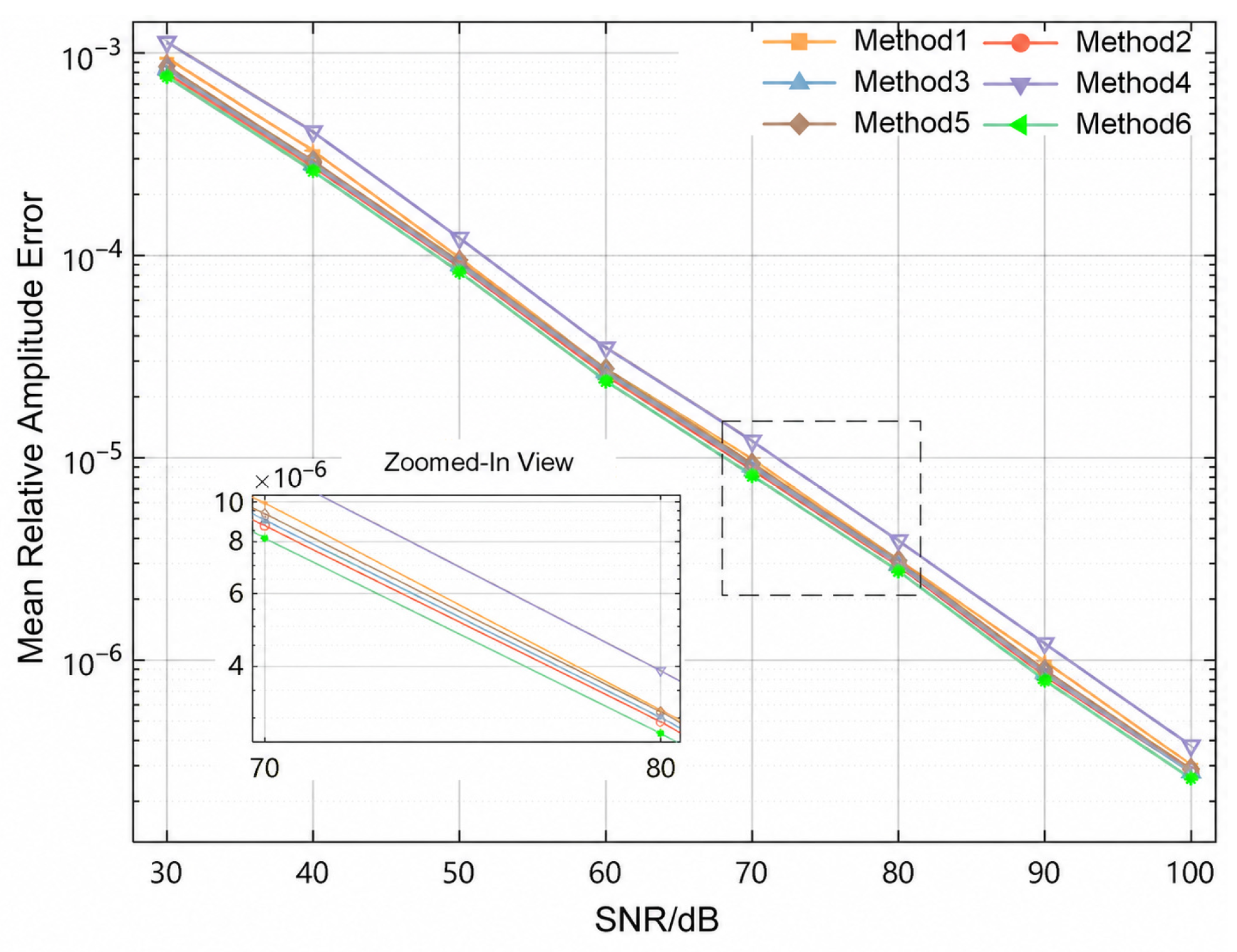
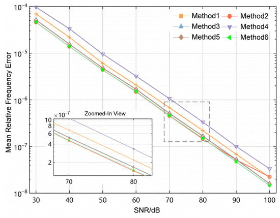
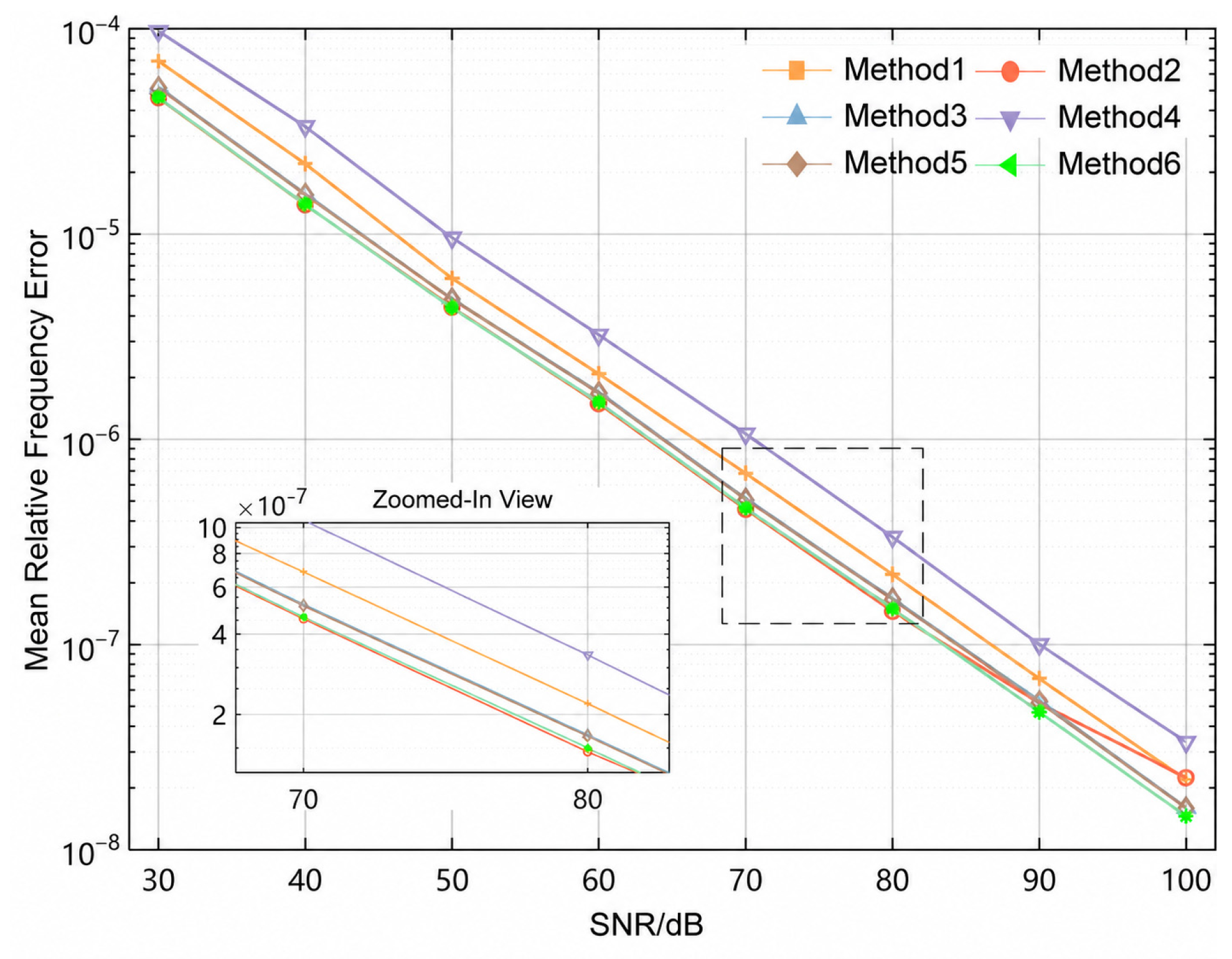
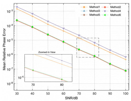
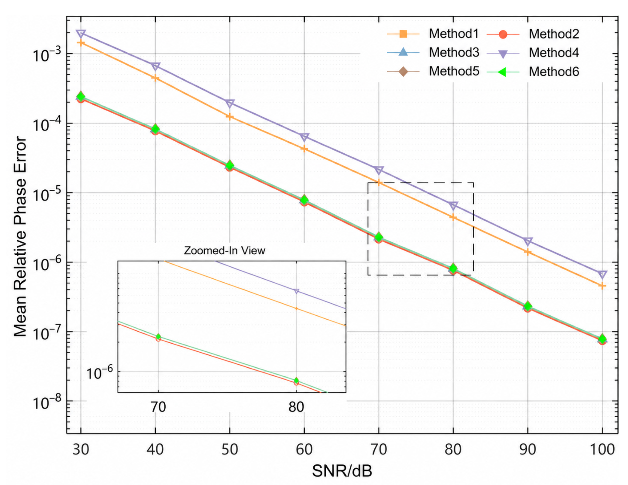
To further evaluate the anti-interference capability of the proposed algorithm under practical operating conditions, Gaussian white noise with different intensities is added to the signal containing harmonic components up to the 21st order. The signal-to-noise ratio (SNR) is varied from 30 to 100 dB with a step size of 10 dB. For each SNR level, the six algorithms are independently tested 200 times, and the average results are calculated. The mean relative error is adopted as the evaluation metric for comparing the final estimation performance.
The performance of the six methods under different SNR conditions is then evaluated. The relative errors in amplitude, frequency, and phase estimation are shown in Figure 8, Figure 9 and Figure 10, respectively.
Figure 8.
Comparison of relative amplitudes errors.
Figure 9.
Comparison of relative frequency errors.
Figure 10.
Comparison of Relative Phase Errors.
As shown in Figure 8, Figure 9 and Figure 10, under white-noise interference at different signal-to-noise ratio (SNR) levels, the estimation accuracy of all methods gradually improves as the SNR increases. Comparison among the six methods shows that the proposed algorithm outperforms the conventional Method 1 and Method 4 from Ref. [29] over the entire SNR range, while its overall performance is comparable to that of Methods 2, 3, and 5. In particular, the proposed method exhibits better robustness in amplitude estimation.
At an SNR of 30 dB, the proposed method yields a mean relative amplitude error of 7.64 × 10⁻⁴, a mean relative frequency error of 4.64 × 10⁻⁵, and a mean normalized wrapped phase error of 2.41 × 10⁻⁴ for the fundamental component. Under noisy conditions, the performance differences among the all-phase methods are smaller than those observed in the noise-free tests.
4.4. Analysis of the Effect of Fundamental-Frequency Fluctuation
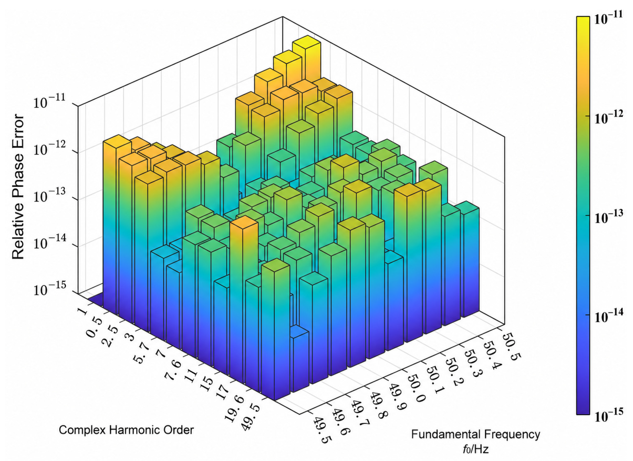
Considering that the fundamental frequency of a practical power grid may vary over time rather than remain absolutely constant, random deviations of ±0.5 Hz or even larger may occur. Such frequency fluctuations can affect the spectral leakage characteristics of individual harmonic components to a certain extent, thereby posing an additional challenge to the accuracy of harmonic detection algorithms. Therefore, simulation analysis under this condition is necessary. By examining the relative errors of the estimated parameters, the detection reliability of the proposed method under fundamental-frequency fluctuations can be further evaluated, thereby evaluating its accuracy under the specified frequency sweep.
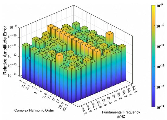
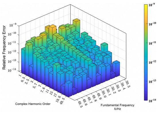
For each value of f0 in the range 49.5–50.5 Hz with a step of 0.1 Hz, the frequency of component i was generated as fi = rif0, where ri is its fixed integer or non-integer order in Table 5. The frequencies listed in Table 5 correspond to the reference fundamental frequency of 50.1 Hz. The component amplitudes and initial phases were held fixed throughout the sweep. Each record contained stationary components at the selected frequencies.
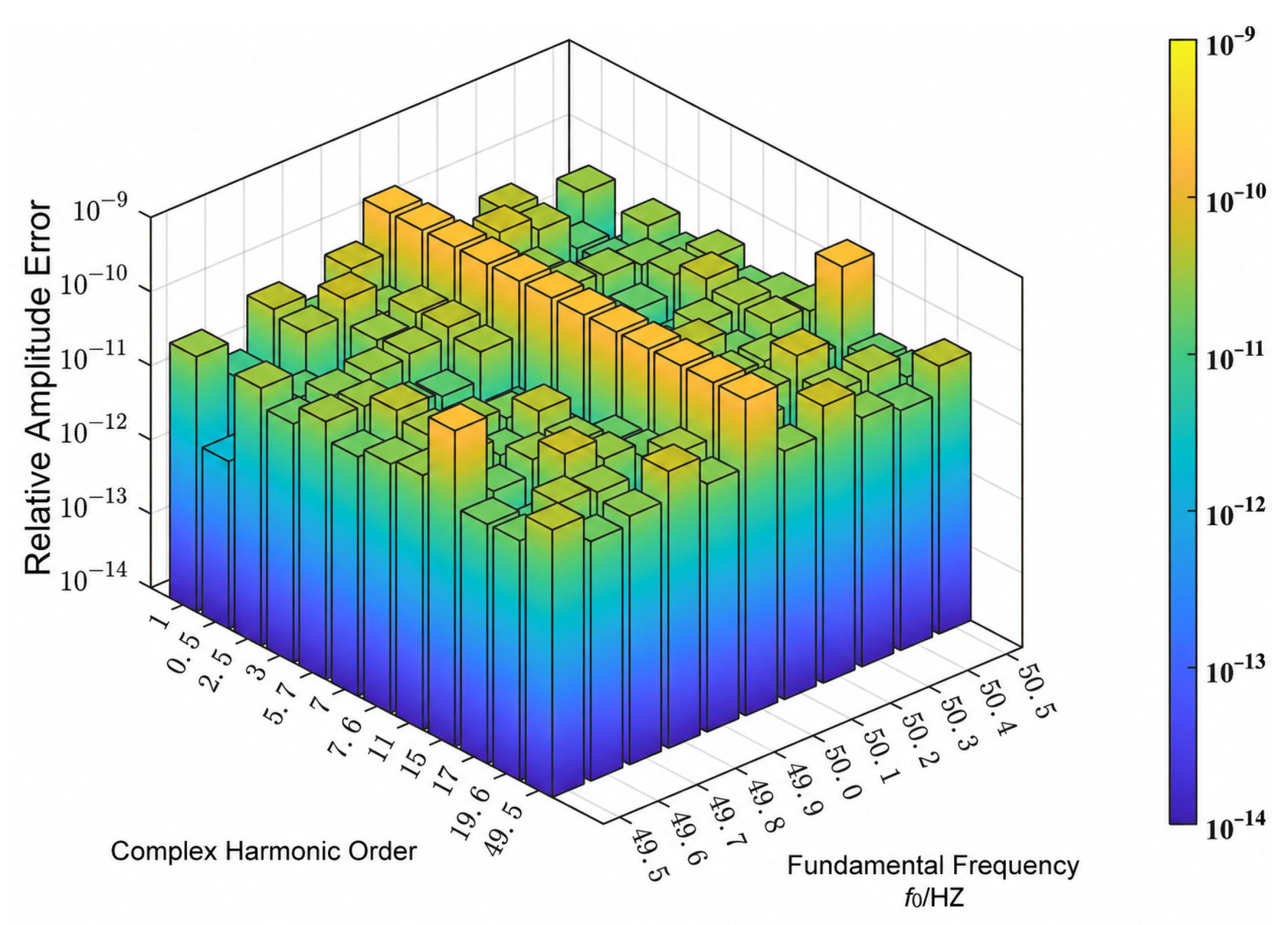
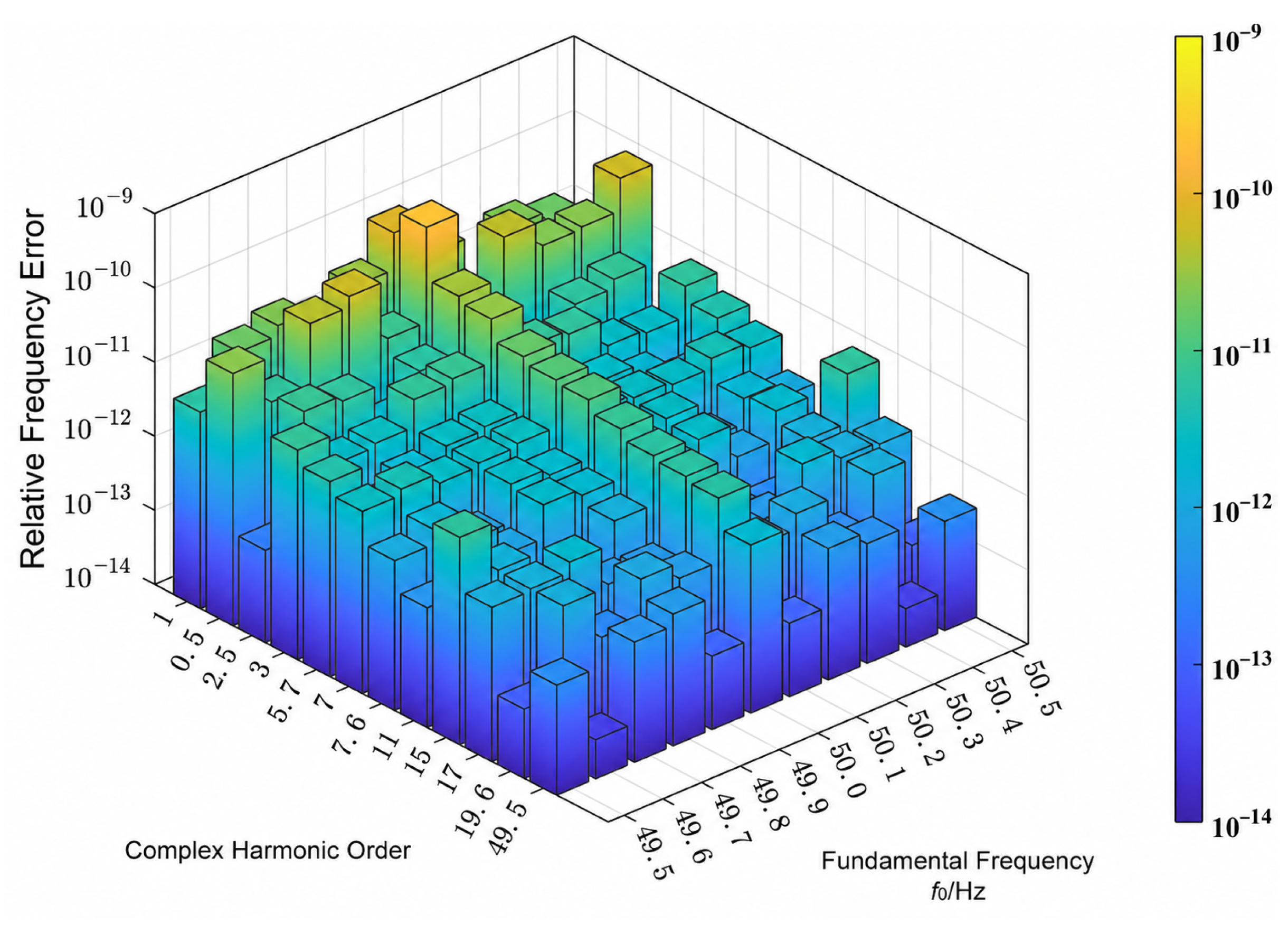
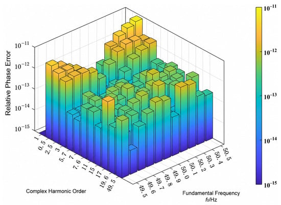
The amplitude, frequency, and phase analysis results of the complex harmonic–interharmonic signal under fundamental-frequency fluctuations are shown in Figure 11, Figure 12 and Figure 13.
Figure 11.
Relative error of amplitude under fundamental frequency fluctuation.
Figure 12.
Relative error of frequency under fundamental frequency fluctuation.
Figure 13.
Relative error of phase under fundamental frequency fluctuation.
4.5. Supplementary Evaluation Under Noise and Nonideal Conditions
To examine whether the improvement extends beyond noise-free interpolation, supplementary experiments were conducted using a double-precision Python3.10/NumPy reproduction of Methods 3 and 6. Both methods used a sampling frequency of 5120 Hz, an FFT length of 2048, and the same 4095 raw samples centered at t = 0. Their weights and correction polynomials were fixed before testing. Method 3 used the six-line weight sequence [1,2,6], ordered from low to high frequency, whereas Method 6 retained its original calibrated configuration. The test signal was a sinusoid with peak amplitude 1, frequency 50.1 Hz, and center-time phase 0.7 rad. At each SNR of 30, 50, and 70 dB, 200 independent Gaussian-noise realizations were shared by both methods. Noise variance was determined from the nominal sinusoidal power, without separately normalizing each realization.
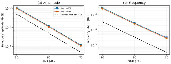
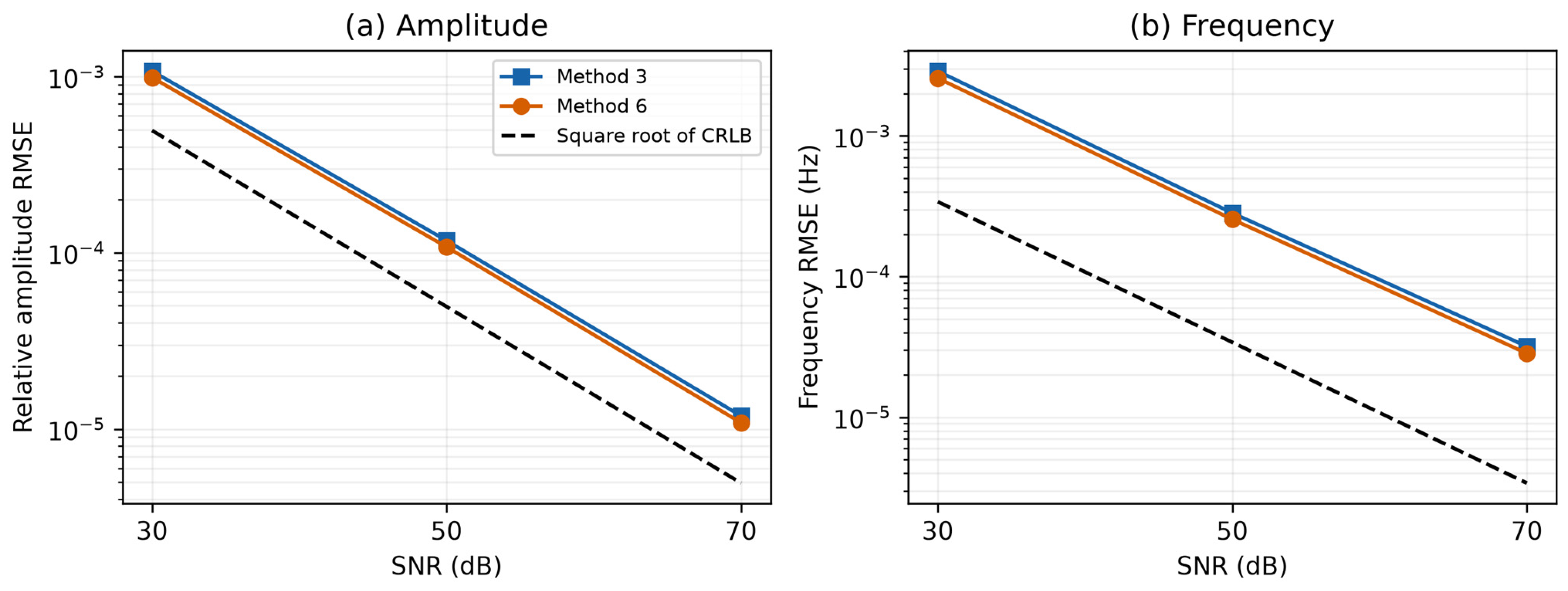
Figure 14 compares the relative amplitude RMSE and frequency RMSE with the square roots of the corresponding Cramér–Rao lower bounds (CRLBs). Across the three SNRs, Method 6 reduced amplitude RMSE by approximately 7.99–8.54% and frequency RMSE by 9.89–10.92% relative to Method 3. Nevertheless, its amplitude and frequency RMSEs remained approximately 2.00–2.20 and 7.49–8.35 times the respective square roots of the CRLB. These results indicate that the improvement over the fixed-weight method persists in the tested noisy conditions.
Figure 14.
Single-tone estimation using 4095 common raw samples and 200 trials per SNR: (a) relative amplitude RMSE; (b) frequency RMSE.
The second experiment used the 21-harmonic signal in Table 3 with a nominal AWGN baseline of 70 dB and 200 paired trials. Three disturbances were introduced separately: 12-bit quantization over [−400, 400) V with a step of 800/4096 V; a constant DC offset of 2.205 V; and amplitude modulation with a depth of 1% and a frequency of 1 Hz. Quantization used nearest-code rounding, and no clipping occurred. No DC removal was applied. Noise variance was determined from the unmodulated signal and held fixed across conditions. Both methods used identical noise records and nominal-frequency search bands. The fundamental and 10th harmonic, with unmodulated peak amplitudes of 220.5 V and 0.8 V, were selected in advance for reporting.
As shown in Table 6, Method 6 retained lower amplitude and frequency RMSEs than Method 3 for both reported components under static AWGN and quantization. With 12-bit quantization, the amplitude-RMSE reductions were approximately 8.34% and 8.32% for the fundamental and 10th harmonic, respectively, while the frequency-RMSE reductions were 10.46% and 10.95%. The constant DC offset produced no discernible additional change at the displayed precision. These results show that the numerical benefit is not confined to noise-free interpolation. However, under amplitude modulation, Method 6 produced larger fundamental-component errors than Method 3, while the ranking differed for the 10th harmonic. The observed advantages therefore apply to the tested stationary conditions and do not establish uniform superiority for dynamic signals, practical instrument accuracy, or standards compliance.
Table 6.
Relative amplitude RMSE and frequency RMSE under selected nonideal conditions at a nominal SNR of 70 dB.
4.6. Computational Cost
Methods 3 and 6 required mean processing times of 0.0972 ms and 0.0980 ms, respectively, to estimate the amplitudes, frequencies and phases of all 21 harmonic components. The similar processing times indicate that the calibrated configuration maintains an online computational cost comparable to that of the fixed-weight all-phase baseline in the tested implementation. Together with the accuracy improvements observed under the investigated stationary conditions, these results support the benefit of offline calibration without requiring online PSO execution.
The reported processing times characterize the desktop MATLAB implementation and should be distinguished from the approximately 0.8 s observation window. Evaluation on embedded platforms remains a direction for future work, with emphasis on computational efficiency, memory requirements and end-to-end latency under practical acquisition conditions. Processing times were measured in MATLAB R2024a on an Intel Core i5-12400 desktop for complete estimation from a 4095-sample record, excluding data acquisition and offline calibration, and averaged over 300 batches of 100 calls per method.
5. Discussion
The results indicate that calibrating the relative spectral-line weights together with the correction functions can reduce deterministic interpolation error for the investigated MSD self-convolution all-phase estimator. Reference [19] provides an established dual-window all-phase interpolation framework, while Ref. [29] demonstrates the use of offline PSO for spectral-line weight optimization. The present work builds on these developments by matching the weighted interpolation and its correction functions to the MSD self-convolution all-phase response under nonnegative normalization constraints. The observed performance should therefore be interpreted in terms of the complete spectral model and calibration procedure, rather than attributed to PSO alone.
The optimized normalized weights are a* = 0.130962417, b* = 0, and c* = 0.869037583, with a validation-set mean relative amplitude error of 2.499004 × 10⁻¹¹. Under the investigated calibration conditions, the central and outer pairs form the selected combination, whereas the intermediate pair receives zero weight. This result illustrates that the contribution of a spectral-line group depends on its interaction with the spectral response and correction functions, rather than solely on its distance from the spectral peak. These observations support calibrating the relative weights together with the correction functions for the specific spectral model. The selected line combination is specific to the investigated calibration conditions and is not claimed to be universally optimal.
The objective-function comparison in Table 2 shows that the choice of calibration objective affects amplitude and frequency accuracy differently. Under the investigated configuration, frequency-only calibration lowers the independent-test frequency RMSE by approximately 38.92% relative to amplitude-only calibration, but increases the mean relative amplitude error to approximately 297 times the amplitude-only value. The three tested joint objectives produce weights close to the amplitude-only solution, with reductions in amplitude error and frequency RMSE below 0.02% and 0.003%, respectively. Among the selected solutions in Table 2, amplitude-only calibration yields the lowest validation-set mean relative amplitude error, with only small differences from the joint settings. Together with the amplitude-focused purpose of the method and the absence of a mixing coefficient, this supports retaining amplitude-only calibration. The slightly lower test amplitude errors of the joint settings do not invalidate this validation-based choice. No claim is made that amplitude-only calibration is universally superior or provides the best frequency accuracy.
The noise-free harmonic and interharmonic tests demonstrate the effect of matching the interpolation weights and correction functions to the MSD dual-window all-phase response. As reported in Section 4.1, the mean relative amplitude error over the 21 harmonic components decreases from 1.099 × 10⁻⁹ for Method 3 to 2.213 × 10⁻¹¹ for the proposed method, a reduction of approximately 97.99%. In the nine-component interharmonic test in Section 4.2, the proposed method has relative amplitude errors of 8.99 × 10⁻¹²–4.16 × 10⁻¹¹ and relative frequency errors of 9.65 × 10⁻¹⁴–1.365 × 10⁻¹¹. These numerical results characterize the interpolation errors under the investigated noise-free conditions and should not be interpreted as achievable accuracy in practical measurements.
Supplementary two-tone tests examined spectral interference using a 50.1 Hz, 220.5 V component and a neighboring component with amplitude ratios of 1, 0.01 and 0.001. Separations ranged from 0.5 to 10 FFT bins, with 200 random-phase trials per condition under noise-free and 60 dB conditions. Peak resolution required two distinct spectral peaks within 0.5 bin of the respective true frequencies. Joint success additionally required both amplitude errors to be within 10% and both frequency errors to be within 0.5 bin. At a three-bin separation and 60 dB, the joint success rate for equal-amplitude components increased from 38.5% for Method 3 to 80.5% for Method 6. However, the peak-resolution rates were identical because the two methods share the same spectrum and peak selection. Weak components near the strong fundamental were not reliably estimated at small separations, and Method 6 did not uniformly reduce their errors. Thus, calibration can improve interpolation in some overlapping-spectrum cases but does not provide a general remedy for unresolved or strongly contaminated components.
The results also show that favorable standalone window characteristics do not necessarily lead to the best final estimation performance. Although some hybrid convolution windows have lower sidelobe levels or faster sidelobe decay than the MSD window, their overall performance is not superior when combined with apFFT and subsequent interpolation. This confirms that window selection should consider not only sidelobe characteristics, but also its compatibility with all-phase processing and the interpolation model.
The white-noise experiment in Section 4.3 covers SNRs from 30 to 100 dB and evaluates the fundamental component of the 21-harmonic signal. At 30 dB, the proposed method has mean amplitude and frequency relative errors of 7.64 × 10⁻⁴ and 4.64 × 10⁻⁵, respectively, and a mean normalized wrapped phase error of 2.41 × 10⁻⁴, expressed without a percentage sign. The performance of the all-phase methods is broadly comparable under noise, so the large reductions in noise-free interpolation error should not be extrapolated to equally large improvements in noisy measurements. The fundamental-frequency sweep in Section 4.4 further examines the estimator over 49.5–50.5 Hz under the stated simulation conditions.
The weights used in this study were calibrated to reduce deterministic interpolation error without specifying an SNR distribution. A supplementary experiment using a predefined mixture of noisy calibration conditions produced a different fixed weight vector and reduced the estimation errors in the tested single-tone noise cases. The original configuration is therefore retained for the stated deterministic-calibration objective and is not claimed to be optimal under noise.
The approximately 0.8 s observation window should be distinguished from the processing times reported in Section 4.6. For estimates referenced to the record center, the final sample becomes available approximately 0.4 s after that reference time, before computation and other implementation overheads are considered. These timing relationships do not constitute measured end-to-end latency. The current configuration has not been evaluated with a 200 ms record or on an embedded platform. Future work will investigate shorter observation windows and embedded implementation, including their effects on estimation accuracy, computational efficiency and acquisition-to-output latency.
Overall, the improvement achieved by the proposed method results from the coordinated interaction among MSD dual-windowing, all-phase spectral analysis, and PSO-based spectral-line weighting. The MSD dual-window suppresses spectral leakage, apFFT improves phase stability, and the optimized line weights enhance frequency-offset and amplitude correction. Therefore, these components should be regarded as an integrated framework rather than independent processing stages. It should also be noted that the optimized weights are obtained under the specific sampling frequency, data length, and MSD dual-window configuration used in this study. Thus, they represent the optimal solution for the investigated conditions rather than a universally optimal weighting scheme for all signal and sampling configurations.
The results characterize the estimation performance under the investigated simulation conditions and do not establish compliance with a specific measurement standard.
6. Conclusions
This paper presents an MSD dual-window apFFT method with PSO-optimized spectral-line weights for harmonic and interharmonic estimation under nonsynchronous sampling. The simulation and computational-cost results lead to the following conclusions:
- (1)
- The MSD window adopted in this study effectively suppresses spectral leakage owing to its favorable sidelobe characteristics. In the MSD dual-window all-phase fast Fourier transform algorithm, the all-phase self-convolution operation further enhances the suppression of spectral leakage, thereby improving the detection accuracy to a certain extent.
- (2)
- The conventional windowed interpolation FFT algorithm is improved by introducing the apFFT. Through periodic segmentation followed by summation, an all-phase periodic extension of the signal is constructed, which reduces spectral leakage. Moreover, owing to the phase-invariance property of apFFT, Phase is estimated from the selected apFFT spectral line using the reference phase compensation and phase-wrapping operation in Equation (23). The PSO-based weight calibration is applied to frequency and amplitude estimation and does not modify the phase estimator. thereby simplifying the algorithm while substantially improving phase estimation accuracy.
- (3)
- A nonnegative normalized multi-line calibration is developed for the MSD self-convolution all-phase spectrum, with the spectral-line weights and their associated correction functions determined consistently. PSO serves as the offline numerical solver. The selected configuration retains the central and outer spectral-line pairs, illustrating how the six-line candidate structure can accommodate an effective subset of lines under the investigated calibration conditions
- (4)
- Compared with the methods reported in other studies, the proposed algorithm exhibits clear advantages in the detection of complex harmonic and interharmonic signals. It also demonstrates good robustness under Gaussian white-noise interference for signals containing harmonics up to the 21st order and under fluctuations in the fundamental frequency, further verifying the effectiveness and superiority of the proposed method.
In summary, the proposed algorithm can accurately detect complex harmonic and interharmonic components. The simulation results demonstrate the effectiveness of the proposed method under the investigated conditions. Validation using measured power-grid signals has not yet been performed and remains a limitation of the present study. Future work will evaluate the method using measured signals and investigate shorter observation windows and embedded implementations, with particular attention to estimation accuracy, processing time, and end-to-end latency.
Author Contributions
Conceptualization, Z.L. and Q.L.; methodology, Q.L. and Z.L.; software, Q.L.; validation, Q.L. and Z.L.; formal analysis, Z.L. and L.W.; investigation, Q.L.; resources, L.W. and Z.H.; data curation, Q.L.; writing—original draft preparation, Q.L.; writing—review and editing, Z.L. and L.W.; visualization, Q.L.; supervision, Z.H. and L.W.; funding acquisition, Z.L. All authors have read and agreed to the published version of the manuscript.
Funding
This research was funded by National Natural Science Foundation of China, grant number 52277012.
Data Availability Statement
The underlying data cannot be shared because of confidentiality restrictions. The signal models, calibration settings, and evaluation procedures are described in the article.
Acknowledgments
The authors would like to express their sincere gratitude to all those who supported this research.
Conflicts of Interest
Lin Wu is employed by State Grid Hubei Electric Power Co., Wuhan, China. The remaining authors declare that the research was conducted in the absence of any commercial or financial relationships that could be construed as a potential conflict of interest.
Abbreviations
The following abbreviations are used in this manuscript:
| FFT | Fast Fourier Transform |
| PSO | Particle Swarm Optimization |
| MSD | Maximum Sidelobe Decay |
| apFFT | All-phase fast Fourier transform |
References
- Zhou, X.; Zhao, Q.; Zhang, Y.; Yang, H. Analysis of the development trend of China’s energy and power system under the dual carbon target: Green electricity substitution and green hydrogen substitution. Proc. CSEE 2024, 44, 6707–6721. (In Chinese) [Google Scholar]
- Wang, P.; Zhang, D.; Zhang, Y. Research and prospects for key digital-intelligent technology applications in new power systems. Power Syst. Prot. Control 2025, 53, 175–187. (In Chinese) [Google Scholar]
- Liu, J.; Hou, X.; Li, S.; Yao, W.; Zhao, W.; Wu, H. A review: Harmonic power measurement methods. China Meas. Test. 2025, 51, 1–12. (In Chinese) [Google Scholar] [CrossRef] [Scilit]
- Uz-Logoglu, E.; Salor, O.; Ermis, M. Online characterization of interharmonics and harmonics of AC electric arc furnaces by multiple synchronous reference frame analysis. IEEE Trans. Ind. Appl. 2016, 52, 2673–2683. [Google Scholar] [CrossRef] [Scilit]
- Zhang, H.; Xiong, J.; Cai, X. Power harmonic analysis based on high-rate oversampling and windowed interpolation FFT. Power Syst. Prot. Control 2024, 52, 105–115. (In Chinese) [Google Scholar]
- Chen, H.; He, Y.; Xiao, J.; Liu, M.; Wang, D. Harmonics detection based on a combination of continuous wavelet transform and discrete wavelet transform. Power Syst. Prot. Control 2015, 43, 71–75. (In Chinese) [Google Scholar]
- Liu, J.; Zhao, W.; Li, S. Compressive sensing empirical wavelet transform for frequency-banded power measurement considering interharmonics. IEEE Trans. Instrum. Meas. 2025, 74, 1503012. [Google Scholar] [CrossRef] [Scilit]
- Garanayak, P.; Naayagi, R.T.; Panda, G. A high-speed master-slave ADALINE for accurate power system harmonic and inter-harmonic estimation. IEEE Access 2020, 8, 51918–51932. [Google Scholar] [CrossRef] [Scilit]
- Deng, Y.; Wang, L.; Li, Y.; Liu, H.; Wang, Y. EhdNet: Efficient harmonic detection network for all-phase processing with channel attention mechanism. Energies 2024, 17, 349. [Google Scholar] [CrossRef] [Scilit]
- Xu, H.; Zhong, Y.; Wang, W.; Ren, Y.; Gu, W.; Ma, H. Prony Broadband Oscillation Signal Measurement Method Based on Order Optimization and Noise Suppression. Proc. CSU-EPSA 2026, 1–12. (In Chinese) [Google Scholar] [CrossRef]
- Wang, Z.; Fu, P.; Huang, L.; Chen, X.; Wang, Z.; Zeng, S. Research on improved harmonic detection method based on ip-iq theory. High Power Laser Part. Beams 2019, 31, 056005. (In Chinese) [Google Scholar]
- Bernard, L.; Goondram, S.; Bahrani, B.; Pantelous, A.; Razzaghi, R. Harmonic and interharmonic phasor estimation using matrix pencil method for phasor measurement units. IEEE Sens. J. 2021, 21, 945–954. [Google Scholar] [CrossRef] [Scilit]
- Harris, F.J. On the use of windows for harmonic analysis with the discrete Fourier transform. Proc. IEEE 1978, 66, 51–83. [Google Scholar] [CrossRef] [Scilit]
- Grandke, T. Interpolation algorithms for discrete Fourier transforms of weighted signals. IEEE Trans. Instrum. Meas. 1983, 32, 350–355. [Google Scholar] [CrossRef] [Scilit]
- Andria, G.; Savino, M.; Trotta, A. Windows and interpolation algorithms to improve electrical measurement accuracy. IEEE Trans. Instrum. Meas. 1989, 38, 856–863. [Google Scholar] [CrossRef] [Scilit]
- Agrež, D. Weighted multipoint interpolated DFT to improve amplitude estimation of multifrequency signal. IEEE Trans. Instrum. Meas. 2002, 51, 287–292. [Google Scholar] [CrossRef]
- Gou, Y.; Shi, K.; Cao, S.; Peng, T.; Kong, F.; Wang, J. Wind farm harmonic analysis based on full-phase hybrid window six-spectral line interpolation. In Proceedings of the 14th International Conference on Power and Energy Systems (ICPES 2024), Chengdu, China, 13–16 December 2024; pp. 424–430. [Google Scholar]
- Li, S.; Ai, X.; Xu, Y. High precision harmonic measurement method based on all phase FFT algorithm. China Meas. Test. 2024, 50, 56–61, 130. (In Chinese) [Google Scholar]
- Lai, T.; Wang, J.; Guo, L.; Duan, C.; Li, N.; Pan, Y.; Geng, X. Harmonic detection algorithm based on four-spectrum-line interpolation of Nuttall dual-window all-phase FFT. Electr. Eng. 2025, 46, 119–123. (In Chinese) [Google Scholar]
- Tan, T.; Chen, W.; Liu, K.; Xiong, N.; Zhang, J.; Wang, J. Harmonic analysis based on time-domain mutual-multiplication window. J. Mod. Power Syst. Clean Energy 2016, 4, 47–53. [Google Scholar] [CrossRef] [Scilit]
- Li, Z.; Hu, T.; Du, Y.; Zhang, T.; Li, Z. Harmonic detection method based on the theory of windows and spectrum line interpolation. Power Syst. Prot. Control 2019, 47, 78–88. (In Chinese) [Google Scholar]
- Wang, X.; Chen, G. An improved harmonic detection method for power quality based on hybrid convolution interpolation. In Proceedings of the 6th International Conference on Energy, Power and Grid (ICEPG 2024), Guangzhou, China, 27–29 September 2024; pp. 1131–1134. [Google Scholar]
- Sun, Z.; He, Z.; Zang, T. A kind of hybrid convolution window and its application in harmonic analysis. Trans. China Electrotech. Soc. 2016, 31, 207–214. (In Chinese) [Google Scholar]
- Cao, Y.; Li, J.; Lin, H.; Yang, Y.; Lu, X.; Zhang, F. Slepian and Parzen mutual convolution window-based interpolation FFT for harmonic analysis method in power system. Electr. Meas. Instrum. 2024, 61, 172–178. (In Chinese) [Google Scholar]
- Li, Z.; Yu, C.; Jiang, W.; Wang, X.; Li, Z. Quadruple spectrum line interpolation FFT harmonic analysis method based on five-term Rife–Vincent(I) window. Electr. Meas. Instrum. 2023, 60, 78–84+98. (In Chinese) [Google Scholar]
- Hua, M.; Chen, J. A high precision approach for harmonic and interharmonic analysis based on six-spectrum-line interpolation FFT. Power Syst. Prot. Control 2019, 47, 9–15. (In Chinese) [Google Scholar]
- Tao, S.; Guo, A.; Zhao, L.; Yin, W. Harmonic detection method of inter-harmonics based on six term window functions with maximum side lobe decay speed and six-spectrum-line interpolation algorithm. Power Capacit. React. Power Compens. 2019, 40, 110–116. (In Chinese) [Google Scholar]
- Zhao, C.; Zhang, D. Doppler signal processing based on mixed convolutional window six spectral lines. Laser Infrared 2024, 54, 734–740. (In Chinese) [Google Scholar]
- Yuan, W.; Li, K.; Luo, Y.; Yin, C.; Xu, A.; Lu, Z.; He, J. Harmonic and interharmonic detection method based on hybrid convolution windows and particle swarm optimization-based spectral line interpolation. Power Syst. Prot. Control 2026, 54, 88–96. (In Chinese) [Google Scholar]

Disclaimer/Publisher’s Note: The statements, opinions and data contained in all publications are solely those of the individual author(s) and contributor(s) and not of MDPI and/or the editor(s). MDPI and/or the editor(s) disclaim responsibility for any injury to people or property resulting from any ideas, methods, instructions or products referred to in the content. |
© 2026 by the authors. Licensee MDPI, Basel, Switzerland. This article is an open access article distributed under the terms and conditions of the Creative Commons Attribution (CC BY) license.