


Abstract
A component-constrained co-design procedure is developed for a high-order quasi-absorptive harmonic filter in 12–20 MHz HF power amplifiers. Nominal ninth-order low-pass and seventh-order high-pass branches combine fourteen selected capacitors with seven adjustable air-core inductors. Connected-network refinement raises minimum simulated 24–80 MHz rejection from 37.5 to 49.3 dB, with minimum harmonic-port transfer changing from 86.6% to 83.3%. Two-sided perturbations identify coil-specific tuning priorities and expose rejection degradation on both sides of the nominal LP2 setting. Prototype insertion loss is 0.16–0.20 dB and minimum rejection is 47.1 dB. At 794 W useful output, five-carrier experiments demonstrate 58.2–66.0 dB H3 improvement. A separate 200 W, 40 dB Port 3 path records 81.4–92.8 W summed carrier and H2–H4 power at that output, reaching 136.5 W during a 473–1000 W scan. System fundamental-output efficiency is 50.7–57.9% with the filter and 61.5–62.6% without it. At 80 MHz, small-signal Port 3 transfer is 65.3% and reflection is 32.6%. A two-hour CW test at 16 MHz and 794 W records a 61.4 °C termination temperature. The results connect high-order LC implementation to quantified tuning and operating trade-offs.
1. Introduction
High-frequency (HF) ocean radars support ocean-current observation and ship tracking, including multifrequency and multistatic operation [1,2]. Deployment and operation practices are important to reliable coastal current measurements [3]. Recent work by the Wuhan University team has addressed radio-frequency monitoring for operating-frequency selection [4], transmit and receive antenna-pattern measurements for multiple-input multiple-output (MIMO) HF surface-wave radar [5], and directional wave-spectrum retrieval using a dual-site radar network [6]. These studies provide the marine-radar application context for the transmitter output network considered here.
The present design serves a 12–20 MHz ocean-radar power amplifier (PA). Its output network must pass the continuous carrier band while suppressing second- through fourth-order harmonics over 24–80 MHz. The narrowest separation is only 4 MHz, between the highest fundamental and the lowest second harmonic. At near-kilowatt output, this transition must be obtained without excessive useful-path loss or uncontrolled harmonic loading of the PA.
A reflective low-pass (LP) filter can provide deep harmonic rejection, but the returned wave changes the PA harmonic loading [7]. Channel-separation networks [8] provide a second path to a resistive load. Weinreich and Carroll demonstrated an LP/high-pass (HP) absorptive filter tested to 1 kW, with basic two- to six-pole designs and resonant traps for additional rejection [9]. Morgan and co-workers developed reflectionless structures and synthesis methods supporting arbitrary ladder prototypes, with zero reflection at both ports and all frequencies under ideal-element conditions [10,11,12]. Lee et al. measured second- and third-order lumped absorptive LP and bandpass prototypes and tabulated prototype values through the fifth order [13].
Related implementations include a multilayer input-reflectionless diplexer-based low-pass filter [14], symmetrical lumped filter/diplexer prototypes [15], an absorptive microstrip bandpass filter [16], and a reflectionless waveguide bandpass filter for high-power applications [17]. Miri et al. coordinated suspended-stripline branches based on thirteenth-order LP and pseudo-HP prototypes at 40–60 GHz using the common-junction admittance condition [18]. These designs establish the context for the present implementation of high-order lumped LC branches with available high-power RF capacitors and adjustable air-core coils.
Practical component selection and parasitic effects constrain LC filter implementation [19]. The present network must coordinate high-order branches across the 4 MHz band separation while preserving low carrier loss. Its resonant sections interact through the common input, so a coil adjustment can improve rejection while changing matching and harmonic transfer. Topology and fourteen nominal capacitor values are selected first, followed by joint refinement of seven inductances in the connected network. This arrangement retains realizable capacitor choices and uses the mechanically adjustable coils to obtain the required response. Section 6 compares branch order, tuning strategy, and experimental performance with representative absorptive filters and diplexers [9,13,18].
Sensitivity analysis is an established tool for filter optimization and tuning [20]. For this prototype, the useful output of the analysis is a link between a response deviation and the coils to inspect during local adjustment. Both perturbation signs are retained because a band extremum can move in frequency and rejection can deteriorate on either side of the nominal setting. The analysis therefore reports the two individual changes together with the central slope. Small-signal and integrated-PA measurements then characterize the assembled response under their respective source, load, and power conditions.
This work provides the following engineering contributions:
- (1)
- A component-constrained procedure realizes nominal ninth-order LP and seventh-order HP branches using fourteen fixed capacitors and seven jointly refined inductances. The controlled V2-to-V3 comparison quantifies an 11.8 dB increase in minimum simulated rejection, from 37.5 to 49.3 dB, together with a change in minimum harmonic-port transfer from 86.6% to 83.3%. Weight and search-bound studies document the selected rejection-prioritized design.
- (2)
- Forty-two individual-inductor perturbations turn the high-order response into coil-specific adjustment guidance. LP2 changes of −1% and +1% degrade minimum rejection by 5.5 and 1.3 dB, respectively, providing quantitative evidence of the tuning sensitivity. LP3/LP4 chiefly affect useful-band matching, while HP1/HP2 govern minimum harmonic-port transfer. Retaining both perturbation signs identifies which response metrics must be checked after each local coil adjustment.
- (3)
- Small-signal transmission and reflection measurements at the three physical ports are combined with PA output harmonics at five carrier frequencies, direct Port 3 spectral power, and system supply-current comparisons. These measurements connect the high-order design to near-kilowatt PA operation and quantify harmonic suppression, routed power, and system efficiency under their stated configurations. The two-hour CW endpoint test and use in ocean radar products provide complementary implementation evidence.
2. Circuit Configuration and Component-Constrained Co-Design
2.1. Requirements and Design Stages
The fundamental interval is 12–20 MHz. H2 occupies 24–40 MHz, H3 occupies 36–60 MHz, and H4 occupies 48–80 MHz, producing a continuous 24–80 MHz harmonic interval. Port 1 is the common input, Port 2 is the useful LP output, and Port 3 is the HP output connected to an internal 50 Ω termination in the completed module. The 20–24 MHz transition is inspected separately because it lies between the useful and harmonic design bands.
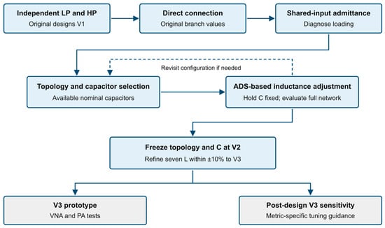
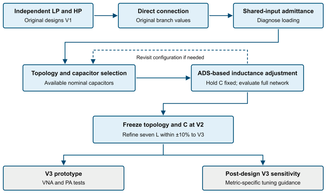
In the design sequence shown in Figure 1, V1 denotes the original independently designed LP and HP circuits. Their branch parameters are retained in the direct-connection reference, with a shared 1 nH connection before the input junction. The branch topology, capacitor configuration, and inductances are then iteratively adjusted using ADS simulations of the complete three-port network to obtain V2. Once the fourteen capacitors and topology are fixed, the seven principal inductances are jointly refined to V3, which supplies the fabrication targets. The ±10% bound applies only to V2-to-V3 refinement. Post-design sensitivity is evaluated around V3.
Figure 1.
Staged design procedure. The V1-to-V2 stage uses ADS simulations of the complete network to guide topology and component adjustments. Dashed feedback indicates the capacitor-selection rule. V3 provides the basis for prototype validation and post-design sensitivity analysis.
2.2. Independent Branches and Shared-Input Loading
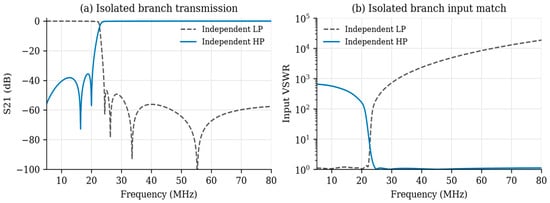
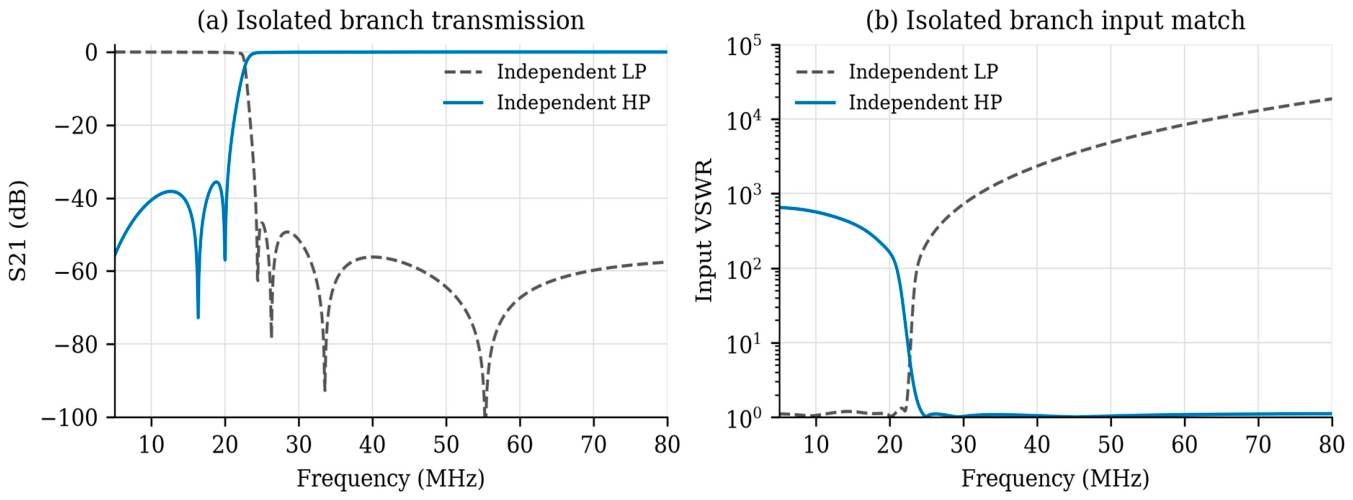
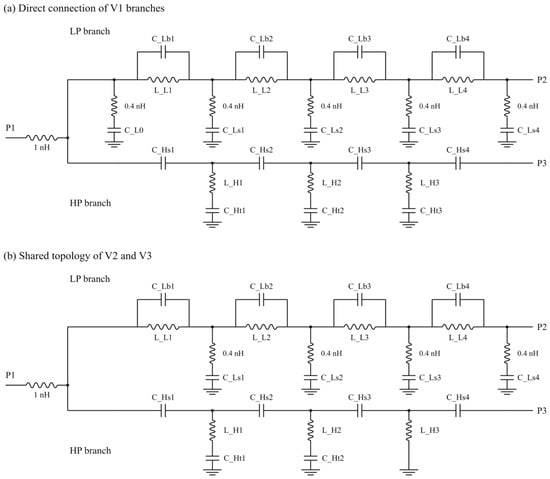
The initial LP circuit has four series inductors bridged by capacitors and five shunt-capacitor branches. The initial HP circuit has four series capacitors and three shunt series-LC branches. These independent branch designs are retained in the original ADS schematic. With 50 Ω source and load impedances, the LP has a maximum simulated insertion loss of 0.13 dB over 12–20 MHz. The HP provides at least 35.6 dB isolation over that interval and no more than 0.35 dB transmission loss over 24–80 MHz. Figure 2 shows their separate responses.
Figure 2.
Native ADS responses of the original independent branches with 50 Ω terminations.
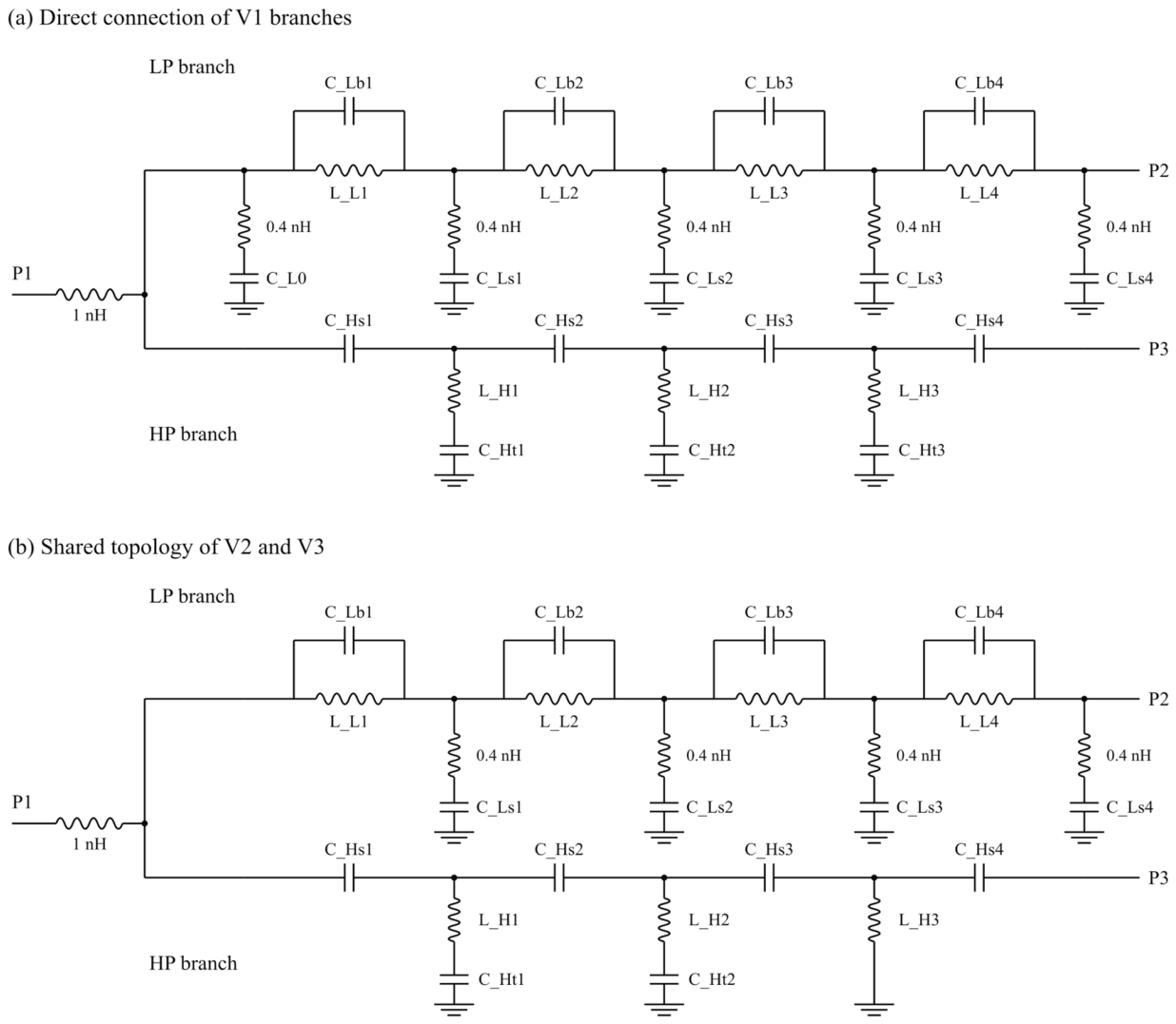
For the direct-connection reference, the LP and HP branches retain their original component values and share one input junction. The 1 nH connection is placed before this junction, as in V2 and V3. Only one external 50 Ω input port is used. The LP and HP outputs become Ports 2 and 3, respectively, and remain matched during simulation. Figure 3a defines this circuit.
Figure 3.
(a) Direct connection of the V1 branches; (b) common topology of V2 and V3. Both circuits include a shared 1 nH connection before the input junction. Element positions increase from input to output. LP1–LP4 correspond to L_L1–L_L4; HP1–HP3 correspond to L_H1–L_H3.
With both output ports terminated in 50 Ω, the branch driving-point admittances add at a common junction reference plane [18]. Let Zc denote a series connection impedance before that plane. For the lumped network without an additional interbranch coupling path, the input and isolated-HP impedances are
where Z0 = 50 Ω. Input matching is evaluated from Zin approaching Z0, including Zc; only when Zc is negligible does this reduce to YJ approaching 1/Z0. At 20 MHz, the original HP input impedance is approximately 0.31 − j5.32 Ω. Its low transmission therefore coexists with substantial reactive loading rather than an open input. Direct connection raises maximum 12–20 MHz loss to 13.85 dB and maximum input VSWR to 59.00.
The common-junction condition [18] is used as a diagnostic in three frequency regions. In the useful band, whether the high-pass branch loads the low-pass path is inspected. In the harmonic band, whether the low-pass branch impedes transfer to Port 3 is inspected. In the transition, reactive cancellation or reinforcement and the resulting mismatch are inspected. Complete-network S21, S31, and input reflection are then evaluated together. Low transmission to Port 2 alone cannot distinguish routing to Port 3 from reflection or dissipation.
2.3. Branch Coordination and Component Selection Using ADS
The shared-input loading identified in Section 2.2 motivates coordination of the connected branches. The LP input shunt-capacitor branch participates in the original independent matching configuration. After connection, it adds capacitive loading at the common junction. Removing this branch reduces that contribution and reconfigures the input matching together with readjustment of the remaining LP and HP elements.
The third HP shunt branch admits a separate simplification. In the original ADS model, its 609.288 nF capacitor has a reactance magnitude of approximately 0.013 Ω at 20 MHz, compared with 28.75 Ω for the series 228.760 nH inductor. Across 12–80 MHz, the capacitive reactance is less than 0.13% of the inductive reactance. The capacitor can therefore be bypassed while retaining the inductor to ground. The resulting topology has fourteen principal capacitors, seven principal inductors, and four 0.4 nH LP shunt-connection inductances, in addition to the shared 1 nH input connection (Figure 3). For each isolated ideal principal-element branch with 50 Ω terminations, the reduced transfer denominator has degree nine for LP and seven for HP. These nominal branch orders exclude the small connection inductances, which remain included in all complete-network simulations.
Capacitor selection and inductance readjustment were coordinated in ADS using the complete connected network. Available nominal capacitor values were selected, and inductances were readjusted to recover useful-band transmission and matching while retaining harmonic rejection and transfer to Port 3. Topology or capacitor changes belong to this V1-to-V2 stage. Once V2 was selected, these choices were fixed, so that the V2-to-V3 comparison isolates the subsequent inductance refinement.
For example, the LP bridge-capacitor sequence changes from 62/180/120/18 pF to 5.6/220/100/36 pF, and the HP series sequence changes to 120/100/82/180 pF. With V2 providing low-loss useful-band transmission, input matching, and harmonic routing, its topology and fourteen capacitors were fixed. The remaining refinement then involved only the seven principal inductances, using the ±10% bounds relative to V2 described in Section 2.4. The selected capacitor values are retained in V3 and fabrication. Table 1 records the topology and capacitor configurations, and Table 2 lists the V1, V2, and V3 inductances.
Table 1.
Topology and capacitor transition. Capacitance is in pF unless nF is stated; V2 and V3 share the selected values.
Table 2.
Main inductance targets for simulation and fabrication, listed by physical position in nH. The direct connection retains the V1 values.
2.4. Fixed-Capacitor Joint Refinement of the Seven Inductors
The V2 topology and fourteen capacitor values are fixed during local refinement. The seven variables are xi = Li/Li,V2, with 0.9 ≤ xi ≤ 1.1. These bounds define the local search region around V2. Both branches remain connected during every evaluation. Table 3 specifies weighted soft response goals; the hard constraints are the selected topology, capacitor values, and inductance bounds. The objective is the weighted mean squared positive target violation:
Table 3.
Soft response targets, their actual optimization windows, and weights. S33 is the reflection coefficient at physical Port 3.
For a lower-bound target, vk = max(0, tk − qk); for an upper-bound target, vk = max(0, qk − tk). Here, qk is the S-parameter magnitude in dB, Nk is the number of samples in the kth window, and W is the sum of weights. Each window is averaged separately before weighting. Rejection goals have weight 1000, compared with 200 for useful-path transmission, matching, and harmonic-port transfer, and 100 for harmonic-port isolation. These are engineering priorities rather than a unique optimum weighting. Convergence of J does not imply satisfaction of all goals, and different weights or bounds can select a different compromise.
The numerical refinement uses an external Python 3.12.14 linear nodal-admittance model and SciPy 1.18.1 bounded trust-region reflective least squares [21]. Native ADS separately verifies the rounded final circuit. Optimization samples 5–80 MHz in 0.25 MHz steps; all goal windows include both endpoints. Four starts comprise V2 and three independent uniform samples within ±5% of its inductances, generated using NumPy 2.5.3 default_rng with seed 20260907.
Solver settings are method = “trf”, ftol=xtol=gtol = 10−9, diff_step = 10−5, two-point numerical differentiation, and linear loss. A wrapper limits each start to 480 complete-network residual evaluations, including numerical-Jacobian evaluations, and retains the lowest score encountered. The four archived runs terminated on ftol after 128, 145, 145, and 160 evaluations.
Each retained unrounded candidate is rescored on a 0.05 MHz grid. The second start has the lowest score on that grid and supplies V3 after rounding to 0.001 nH. This reporting precision is not a hardware adjustment tolerance. The four final scores are approximately 6.11008. Similar scores across these starts do not prove a global optimum. The 30–32 MHz gap between rejection-goal windows is included in full-band performance evaluation.
A supplementary numerical study changes the two rejection weights together by factors of 0.5 and 2 while retaining the remaining weights, and repeats the search with ±5%, ±15%, and ±20% bounds. Each case uses the same four starting vectors and a maximum of 480 complete-network evaluations per start, followed by 0.05 MHz rescoring. These are external linear-model comparisons; the fabricated circuit remains V3. Halving and doubling the rejection weights give minimum rejections of 48.75 and 49.93 dB, with minimum T3 of 83.98% and 82.63%, respectively. The ±10%, ±15%, and ±20% searches return essentially the same retained local compromise.
3. Design Evolution and Performance Trade-Offs
3.1. Native Simulation Conditions
Native ADS 2027 S-parameter simulations use real 50 Ω port references over 5–100 MHz in 0.05 MHz steps, with a separate 0.01 MHz V3 sweep for comparison with measurement. The prescribed finite-Q parameters are QL = 500 and QC = 1000; they are not measured broadband component properties. For INDQ_Z Mode 1 with zero dc resistance, series resistance is 2πfL/QL. CAPQ Mode 1 uses a parallel-loss model defined by its reference frequency [22,23]. The initial high-pass circuit uses a 30 MHz reference, whereas the low-pass, V2, and V3 circuits use 6 MHz. Thus, the V1-to-V2 stage includes topology, component, and loss-setting changes. The V2-to-V3 stage retains identical capacitor and loss models.
For excitation at Port 1 with the other ports matched, power accounting separates input reflection R, transfer to Port 2 (T2), transfer to Port 3 (T3), and modeled internal dissipation D:
Rejection is −20 log10|S21| and describes suppression of transmission to the useful output at a harmonic frequency. T3 is power delivered to a matched termination at Port 3; it equals load absorption only for the stated matched termination. D describes loss inside the passive circuit model and excludes the Port 3 load. High rejection therefore does not establish high absorption. In measurements, 1 − R − T2 − T3 is a power-balance residual that also contains measurement error. The term quasi-absorptive denotes frequency-dependent routing with residual reflection, rather than ideal reflectionless behavior.
3.2. Stage Comparisons
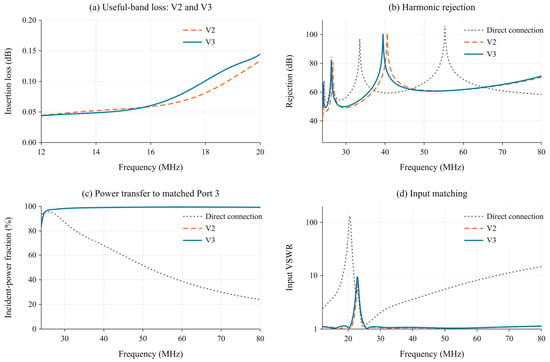
Table 4 and Figure 4 compare the direct-connected reference, V2, and V3 using native ADS simulations. Direct connection of the original branches gives 13.85 dB maximum passband loss and 59.00 maximum passband input VSWR. The complete V2 redesign reduces these values to 0.13 dB and 1.11. This comparison documents the recovery from the original connection; it does not isolate a single design operation. The V2-to-V3 comparison does isolate the effect of changing seven inductances under fixed topology, capacitors, and loss models.
Table 4.
Native ADS complete-network comparison. Extrema are evaluated separately within each stated band.
Figure 4.
Native ADS responses of the direct connection, V2, and V3: (a) useful-band loss of V2 and V3; (b) harmonic rejection; (c) power transfer to matched Port 3; and (d) input matching. The direct-connection passband loss is listed in Table 4.
Fixed-capacitor refinement raises minimum 24–80 MHz rejection from 37.5 to 49.3 dB. Maximum passband loss changes from 0.13 to 0.14 dB, minimum T3 decreases from 86.6% to 83.3%, and maximum harmonic-band input VSWR increases from 1.67 to 1.94. The transition-band maximum VSWR increases from 7.43 to 9.41. V3 is selected to prioritize worst-case harmonic rejection while retaining low carrier loss and a separate harmonic-transfer path. On the common 0.05 MHz evaluation grid, J decreases from approximately 8.03 to 6.11. The 49.3 dB minimum remains below the 50 dB soft goal at some frequencies in 24–30 MHz, and the −65 dB goal is not met throughout 32–80 MHz. The loss goal is also exceeded at some frequencies. Table 4 reports the achieved compromise; the weight and search-bound comparisons in Section 2.4 show its dependence on the selected priorities.
Recalculation of Equation (2) from the rounded native ADS response gives J ≈ 6.110. The 32–80 MHz rejection term contributes approximately 74.7% of this residual score, useful-band input matching 12.9%, and harmonic-port matching 10.9%. These contributions show which violations remain important after refinement. The weight comparisons quantify how changing priorities alters the selected compromise; scores computed with different weights are not directly comparable.
The V3 baseline has its lowest T3 and highest harmonic-band input VSWR at 24 MHz. At that frequency, approximately 83.3% of incident power reaches Port 3, 10.2% is reflected, and the remainder is predominantly model loss. The larger reflection peak in the 20–24 MHz transition is evaluated separately. A denser 0.01 MHz baseline sweep gives 49.31 dB minimum rejection, consistent with the 0.05 MHz evaluation grid at the reporting precision.
4. Inductance Sensitivity and Tuning Implications
4.1. Perturbation Method
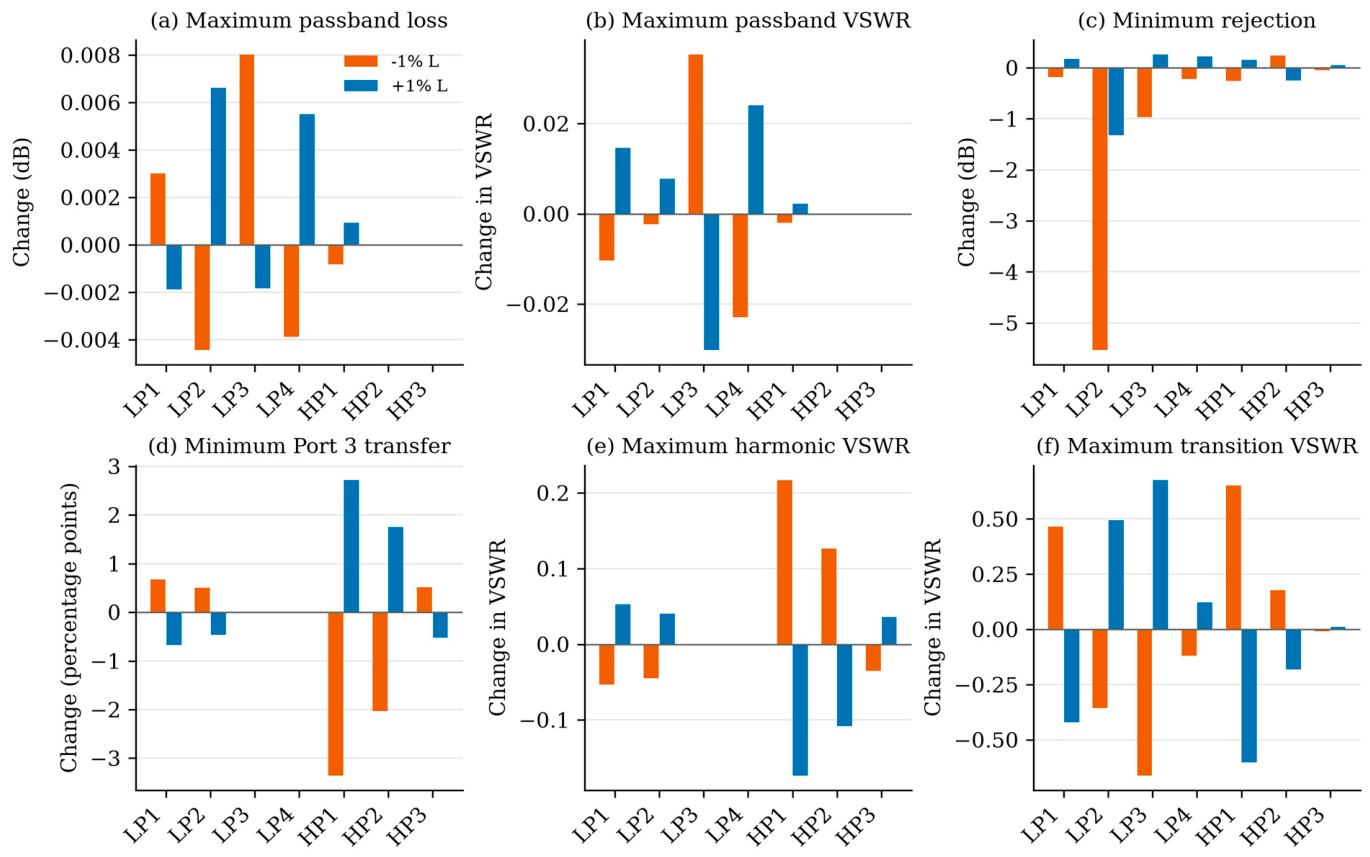
Each principal V3 inductor is varied individually by ±0.5%, ±1%, and ±5%, giving 42 native ADS simulations with all other parameters fixed. These runs are post-design perturbations, not optimization iterations or a statistical yield analysis. The metrics are maximum 12–20 MHz insertion loss and input VSWR, minimum 24–80 MHz rejection and T3, and maximum input VSWR in the harmonic and transition bands. Mutual coupling and parasitic changes caused by physically moving a coil are not included in these perturbations.
For metric M, a finite-difference sensitivity per one percentage point of inductance is defined as
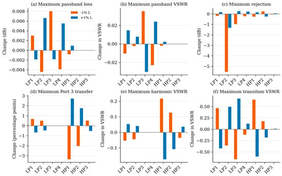
where h is the fractional perturbation. Absolute changes from nominal for both signs are retained together with this slope. Band extrema can shift in frequency, so the resulting metric can be non-smooth. Sensitivities are compared within each metric using its stated units. Figure 5 shows the one-sided ±1% changes.
Figure 5.
Simulated changes from V3 under individual −1% and +1% inductance perturbations. T3 changes are percentage points. Positive changes are favorable for rejection and T3, but unfavorable for loss and VSWR.
4.2. Rejection and Useful-Band Matching
LP2 is the most critical inductor for worst-case harmonic rejection under the tested local perturbations. Its −1% and +1% changes reduce minimum rejection from 49.3 dB to 43.8 and 48.0 dB, respectively. Even the ±0.5% cases reduce the minimum to 46.3 and 48.6 dB. The critical frequency changes from 24.75 MHz at nominal to 24.00 MHz for −1% and 24.65 MHz for +1%. The positive central slope therefore conceals two-sided degradation relative to nominal. LP2 should therefore be maintained near its nominal value during local coil adjustment.
LP3 and LP4 have the largest ±1% effects on maximum passband input VSWR. Increasing LP3 by 1% reduces the maximum from 1.15 to 1.12, whereas decreasing it raises the maximum to 1.19. Increasing LP4 raises it to 1.17, while decreasing LP4 lowers it to 1.13. These directions are local: a +5% LP3 change instead increases passband loss to 0.21 dB and VSWR to 1.25. LP1 and LP4 also affect rejection and the transition response.
4.3. Harmonic Routing and Coil Adjustment Guidance
HP1 and HP2 dominate the minimum harmonic-port transfer. Increasing HP1 by 1% raises minimum T3 from 83.3% to 86.0% and reduces maximum harmonic-band VSWR from 1.94 to 1.76; decreasing HP1 by 1% lowers T3 to 79.9% and increases VSWR to 2.15. Increasing HP2 by 1% raises T3 to 85.0% and reduces VSWR to 1.83, while slightly reducing minimum rejection to 49.1 dB. HP3 has a smaller opposing effect: decreasing it by 1% increases T3 to 83.8%. The ±5% cases show stronger asymmetry; for example, decreasing HP1 by 5% reduces minimum T3 to 61.4%.
The nominal-model results in Table 5 identify LP2 as the first coil to inspect when rejection deteriorates, LP3/LP4 when passband matching shifts, and HP1/HP2 when minimum harmonic-port transfer decreases near the lower band edge. Changing turn spacing can affect inductance, parasitic capacitance, and intercoil coupling simultaneously. The adjustment procedure therefore checks both directions and uses complete-network S21, S31, and input VSWR to accept each trial around V3.
Table 5.
Local tuning recommendations based on simulated individual-inductor perturbations around V3.
5. Prototype Implementation and Experimental Validation
5.1. Capacitors, Coils, and Assembly
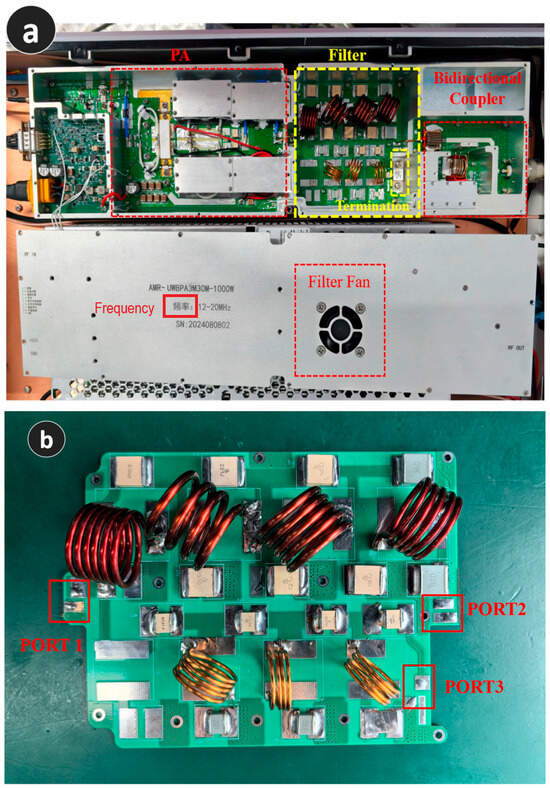
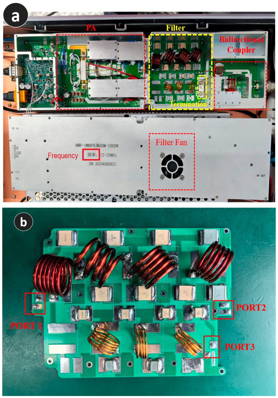
The prototype follows V3 in Table 2 and uses a 100 × 110 mm FR-4 board installed in a 465 × 115 mm PA module. The LP and HP branches use 100E high-power RF capacitors and 700C series capacitors, respectively, from American Technical Ceramics (ATC, USA). The fitted capacitors have nominal tolerances of ±2% or ±5%, depending on the component. After small-signal characterization, Port 3 is connected to a 50 Ω, 250 W RFP-250-50TC termination attached to the metallic housing and cooled by the module fan during normal operation. Figure 6 shows the assembly. The capacitances in Table 1 and these series names specify the selected nominal components. Allowable RF voltage and current depend on capacitance, termination style, frequency, and thermal conditions in the manufacturer data.
Figure 6.
(a) PA module with the integrated filter; (b) filter prototype. Port 3 is connected to the internal matched termination after small-signal characterization.
The dominant third harmonic supplied a preliminary termination-sizing reference. At maximum measured output without the filter, attenuation-corrected spectra correspond to third-harmonic powers of 128, 145, and 144 W at 13, 16, and 19 MHz. A nominal 250 W termination was selected on this basis. These unfiltered values are not measurements of power absorbed by the termination after filter insertion. Actual dissipation depends on the PA-generated spectrum, harmonic routing, load matching, and thermal mounting conditions.
With the nominal capacitors fixed, air-core coils were initially sized using an inductance formula. The LP coils use 2 mm diameter enameled copper wire and have a coil diameter of 23 mm; the HP coils use 1 mm diameter enameled copper wire and have a coil diameter of 15 mm. Individual readings from a TH2816A+ inductance–capacitance–resistance (LCR) meter at a test frequency of 200 kHz guided preliminary adjustment by changing turn spacing to obtain the target inductances. After soldering, both transmission paths and input VSWR were measured with the VNA, and subsequent adjustments used the complete-network response. The 200 kHz readings do not establish the broadband in-circuit inductance or Q, and Table 2 lists nominal design targets rather than independently verified broadband coil parameters.
At 1 kW into a matched 50 Ω load, the reference voltage and current are approximately 224 V rms and 4.47 A rms. A carrier-only linear-model calculation normalized to 1 kW useful output gives substantially higher internal stresses: the largest calculated coil voltage is 505 V rms at LP3, and the largest coil current is 11.10 A rms at LP2. These values use prescribed Q parameters and exclude harmonic excitation, self-resonance, and mutual coupling; they do not establish actual RF rating margins from the capacitor voltage marking alone. Termination power capability also depends on the specified mounting and temperature derating.
5.2. Measurement Conditions
Small-signal characterization used a Rohde & Schwarz ZNB40 vector network analyzer: Rohde & Schwarz GmbH & Co. KG, Munich, Germany. VNA before permanent connection of the internal termination. Two-port through–reflect–match (TRM) calibration was used with a 12–90 MHz sweep in 0.01 MHz steps, 0 dBm source power, and 1 kHz IF bandwidth. For S21, physical Port 3 was terminated in 50 Ω; for S31, Port 2 was terminated in 50 Ω. Input reflection was measured with both output ports matched. Supplementary S22 and S33 measurements used the same calibration and sweep settings, with the other two physical ports terminated in 50 Ω. Here, S22 and S33 refer to the physical useful and harmonic ports, respectively. All reported small-signal data characterize the V3-based prototype.
For useful-output spectral measurements, the filter was installed between the amplifier section and the output bidirectional coupler, with the internal 50 Ω, 250 W termination connected to Port 3. A Keysight N5171B Keysight Technologies, Inc., Santa Rosa, CA, USA. supplied CW excitation, and a Keysight N9020A Keysight Technologies, Inc., Santa Rosa, CA, USA. measured output spectra with 10 dB internal input attenuation and 1 kHz resolution bandwidth (RBW). Total external measurement-path attenuation was 60 dB and was compensated before testing. The recorded analyzer-input background under these settings was approximately −120 dBm, providing the reference for evaluating the weakest useful-output harmonics.
Experimental harmonic measurements cover carrier frequencies of 12, 13, 16, 19, and 20 MHz. Levels at the useful output are expressed in dBc relative to the measured fundamental of each configuration. The configuration-specific curves are interpolated in fundamental output power to a common 59 dBm, with approximately 794 W. Harmonic improvement is the unfiltered dBc level minus the filtered level at that output. The 0.01 dBm summary grid is an interpolation grid rather than a count of independent repetitions.
For an additional Port 3 measurement, the internal 250 W termination was replaced by a 200 W rated attenuator with 40 dB attenuation connected to the spectral measurement path. The measured Port 3 powers are corrected for attenuation and referred to the Port 3 input plane. Carrier leakage and H2–H4 were recorded while useful fundamental output was scanned from 56.75 to 60.00 dBm, with approximately 473–1000 W. This substituted-load configuration is reported separately from the useful-output and original-termination thermal tests.
The system has a single 48.2 V DC input. Supply-current records before and after filter installation are aligned to the useful-output power grid and used to calculate system fundamental-output efficiency. No separate final-stage drain-current measurement is assumed.
5.3. Small-Signal Results
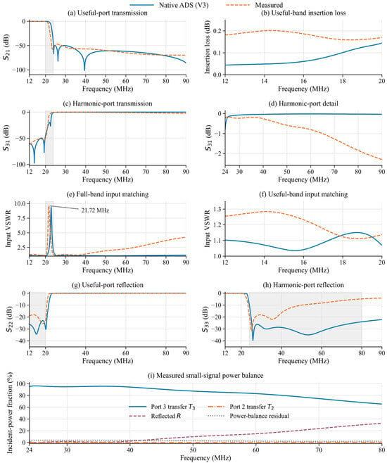
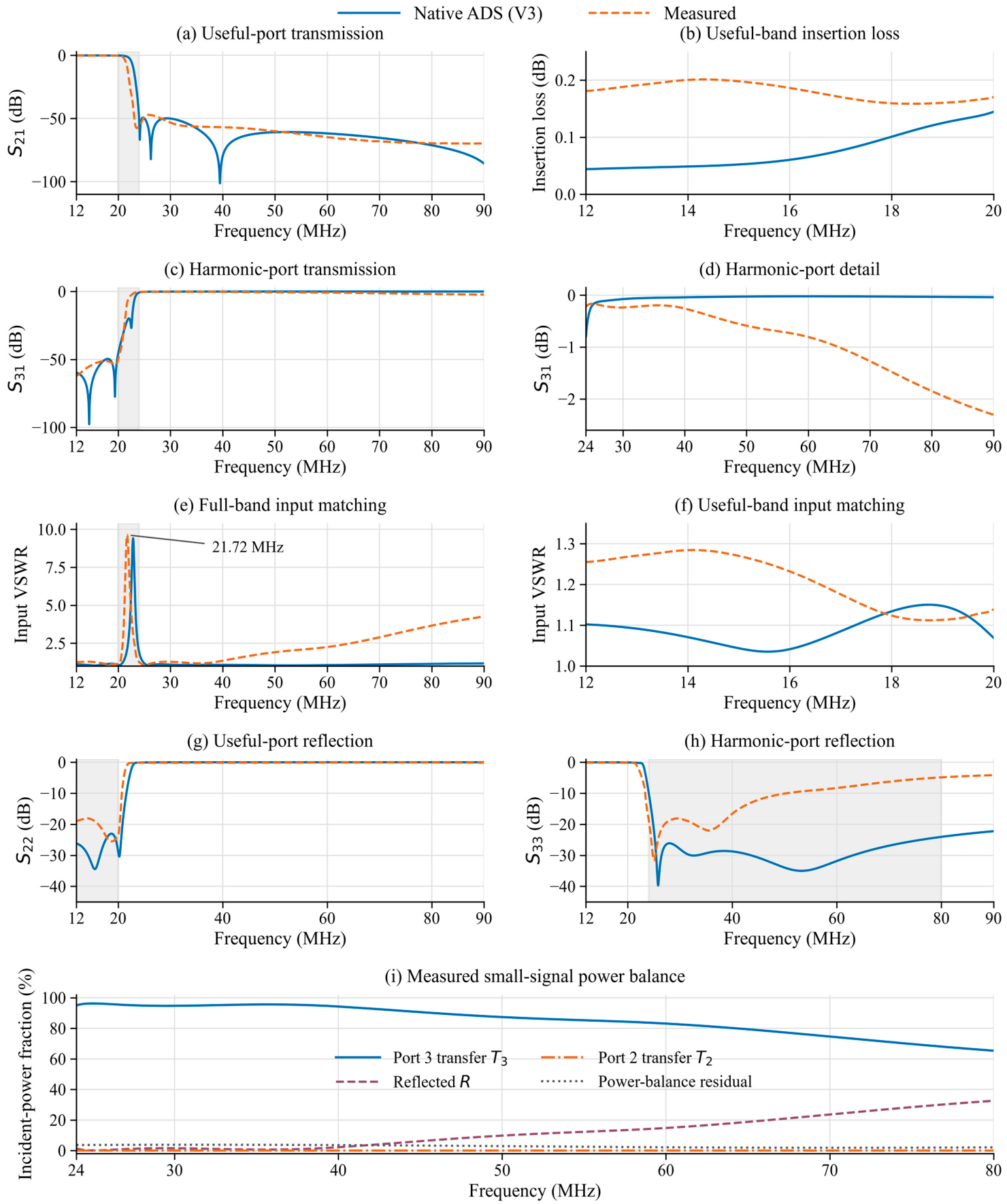
Figure 7 compares native ADS simulations and measured small-signal responses over 12–90 MHz. The VNA data and dense V3 simulation use 0.01 MHz steps. Table 6 evaluates extrema within their stated bands. Over 12–20 MHz, measured insertion loss is 0.16–0.20 dB, compared with 0.04–0.14 dB in the nominal model. Maximum input VSWR is 1.28, compared with 1.15. Measured S31 remains below −50.2 dB in the useful band, indicating isolation of the harmonic port from the fundamental. Figure 7g,h adds the measured and simulated output-port reflection responses. Return loss is defined as −20 log10|Sii|, so larger positive values indicate better matching.
Figure 7.
Native ADS simulations and measured small-signal responses: (a) S21 over 12–90 MHz; (b) insertion loss over 12–20 MHz; (c) S31 over 12–90 MHz; (d) S31 detail over 24–90 MHz; (e) input VSWR over 12–90 MHz; (f) input VSWR over 12–20 MHz; (g) S22 at the useful output; (h) S33 at the harmonic output; and (i) measured small-signal power balance, with all other ports matched. Gray bands indicate the 20–24 MHz transition in (a,c,e), the useful band in (g), and the harmonic band in (h). The power-balance residual includes internal loss and measurement error. Frequencies above 80 MHz lie beyond the harmonic design interval.
Table 6.
Measured small-signal response and V3 simulation comparison. Extrema are evaluated independently within each frequency interval; the 20–24 MHz transition is listed separately.
Across 24–80 MHz, the measured minimum rejection is 47.1 dB at 25.73 MHz, compared with 49.3 dB at 24.77 MHz for V3. The narrow simulated rejection maxima are not reproduced with the same depth in the measured response. At 24 MHz, measured S31 and input VSWR are −0.23 dB and 1.27, compared with −0.80 dB and 1.94 for V3. At 80 MHz, the corresponding measured values are −1.85 dB and 3.66, compared with −0.03 dB and 1.14 for V3.
At 80 MHz, measured T3 is approximately 65.3% and input reflection R is 32.6%, compared with 99.3% and 0.4% in the nominal model. The measured power-balance residual is approximately 2.1%, with negligible T2. Thus, reflection accounts for most of the power not transferred to Port 3. At 24 MHz, measured T3 and R are approximately 94.9% and 1.4%, with a residual of 3.6%; at 40 MHz, they are 94.2%, 2.2%, and 3.6%, respectively. By 60 MHz, T3 decreases to 83.1% and R increases to 14.8%. Figure 7i shows this frequency dependence. These fractions use small-signal measurements with matched external terminations; the residual is not an independently measured heat dissipation.
Measured useful-port return loss is at least 18.1 dB over 12–20 MHz. Harmonic-port return loss reaches approximately 4.9 dB near 80 MHz, confirming degraded upper-band port matching. Input VSWR peaks at 9.63 at 21.72 MHz in the transition, compared with 9.41 at 22.86 MHz in simulation, and reaches 4.25 at 90 MHz beyond the design interval. Frequency shifts and upper-band mismatch therefore accompany, rather than contradict, the deep rejection measured at Port 2.
The model uses fixed nominal elements and prescribed Q values. Actual frequency-dependent impedances, coil self-capacitance and resonance, mutual coupling, interconnects, and reference-plane differences can change matching and transfer. One-factor numerical scenarios examine global QL reductions, 3 pF self-capacitance across LP2 or HP1, and LP2–LP3 coupling coefficients k = ±0.02. The nominal external model agrees with native ADS at the checked frequencies to within 3.2 × 10⁻⁵ in complex S. The scenario parameters are illustrative assumptions, not measured or fitted parasitics.
Reducing QL from 500 to 100 raises modeled maximum useful-band loss from 0.145 to 0.628 dB, but leaves 80 MHz reflection below 0.5%. A 3 pF HP1 self-capacitance raises that reflection to about 1.17%, still far below the measured 32.6%. Weak LP2–LP3 coupling can strongly degrade rejection without reproducing the upper-band mismatch. These tests show that omitted interactions can matter and that a simple global-Q reduction is insufficient; they do not identify a unique physical cause of the measured discrepancy.
The small-signal measurements establish low fundamental-path loss, harmonic rejection, and frequency-dependent transfer to a matched harmonic termination. At 80 MHz, corresponding to H4 of a 20 MHz carrier, substantial residual reflection means that the PA sees a nonideal harmonic load. Direct high-power Port 3 measurements in Section 5.5 quantify transferred harmonic power under the substituted attenuation-path condition. They complement, rather than replace, the matched-port small-signal characterization.
5.4. Harmonic Suppression at Equal Useful Output
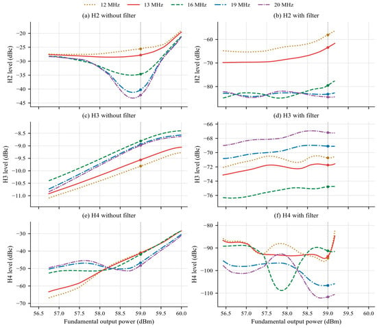
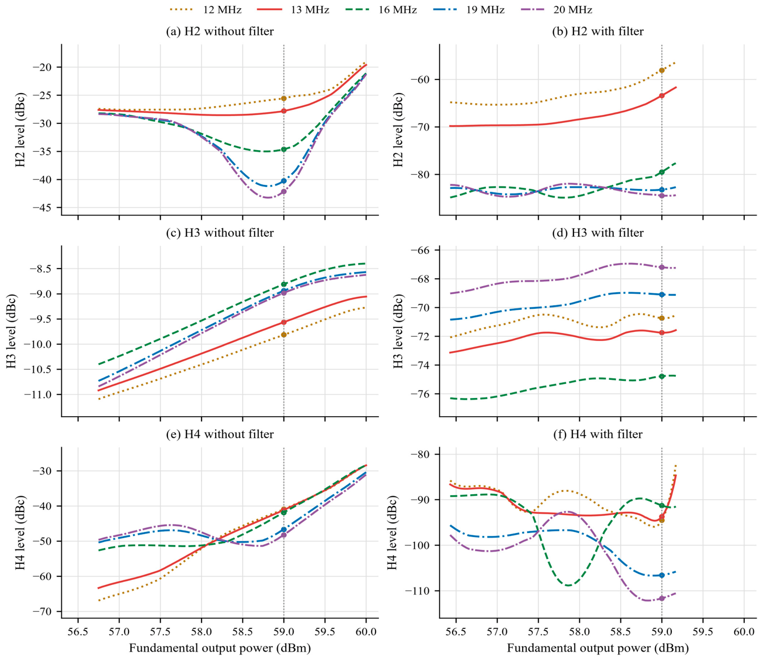
Figure 8 shows experimental second-, third-, and fourth-harmonic levels at 12, 13, 16, 19, and 20 MHz. The horizontal axis is measured fundamental output power for each configuration. All curves include 59 dBm, approximately 794 W. Table 7 compares all five carrier frequencies at this common output; the boundary-frequency results are experimental measurements.
Figure 8.
Experimental harmonic levels versus fundamental output power at 12, 13, 16, 19, and 20 MHz: (a,b) H2; (c,d) H3; and (e,f) H4. Left and right columns show measurements without and with the filter. Curves use the configuration-specific aligned power ranges; the markers and vertical grey dashed lines indicate a fundamental output power of 59 dBm.
Table 7.
Experimental harmonic levels at five carrier frequencies, interpolated in fundamental output power to 59 dBm (approximately 794 W). Improvement is calculated from unrounded values before rounding to one decimal place.
At 794 W useful output, H3 is the strongest unfiltered harmonic. Its improvement is 60.9, 62.2, 66.0, 60.2, and 58.2 dB at 12, 13, 16, 19, and 20 MHz, respectively. H2 improvement spans 32.5–44.9 dB and H4 improvement spans 49.4–63.4 dB. Equal-output comparison fixes the dBc reference but does not ensure unchanged PA-generated harmonics, drive level, or internal operating state.
At 13 MHz, measured small-signal rejection at 26 MHz is 47.17 dB, whereas H2 improvement is 35.61 dB. If insertion did not change the PA-generated harmonic-to-fundamental ratio, harmonic attenuation minus the 0.19 dB fundamental loss would predict approximately 46.98 dB improvement. The remaining difference is about 11.4 dB. Similar H2 differences occur at 16 and 19 MHz. Changing the harmonic load and drive required for equal output can alter PA-generated harmonics, while measurement-chain effects may also contribute. The available spectra do not uniquely distinguish these mechanisms.
The lowest useful-output harmonic level in Table 7 is H4 at a 20 MHz carrier, 80 MHz, at −111.7 dBc. With a 59 dBm fundamental and 60 dB external path loss, this corresponds to approximately −112.7 dBm at the analyzer input, about 7.3 dB above the recorded −120 dBm background. H4 at a 19 MHz carrier is −106.6 dBc, corresponding to −107.6 dBm at the analyzer and a 12.4 dB separation. The 80 MHz result consequently has less noise margin. The uncertainty of these weak harmonic measurements includes contributions from attenuation calibration, detector response, and analyzer noise.
In the original internal-termination configuration, the previously recorded maximum CW outputs at 13, 16, and 19 MHz are approximately 827, 860, and 977 W. The aligned useful-output spectral curves are used for the common-output comparison rather than to redefine each carrier’s maximum. The separate Port 3 attenuation-path scan reaches 60 dBm useful output and is discussed under its own load condition.
5.5. High-Power Measurements at the Harmonic Port
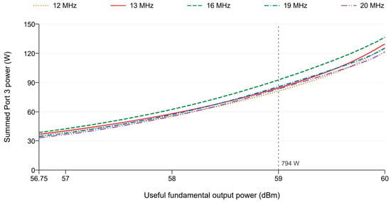
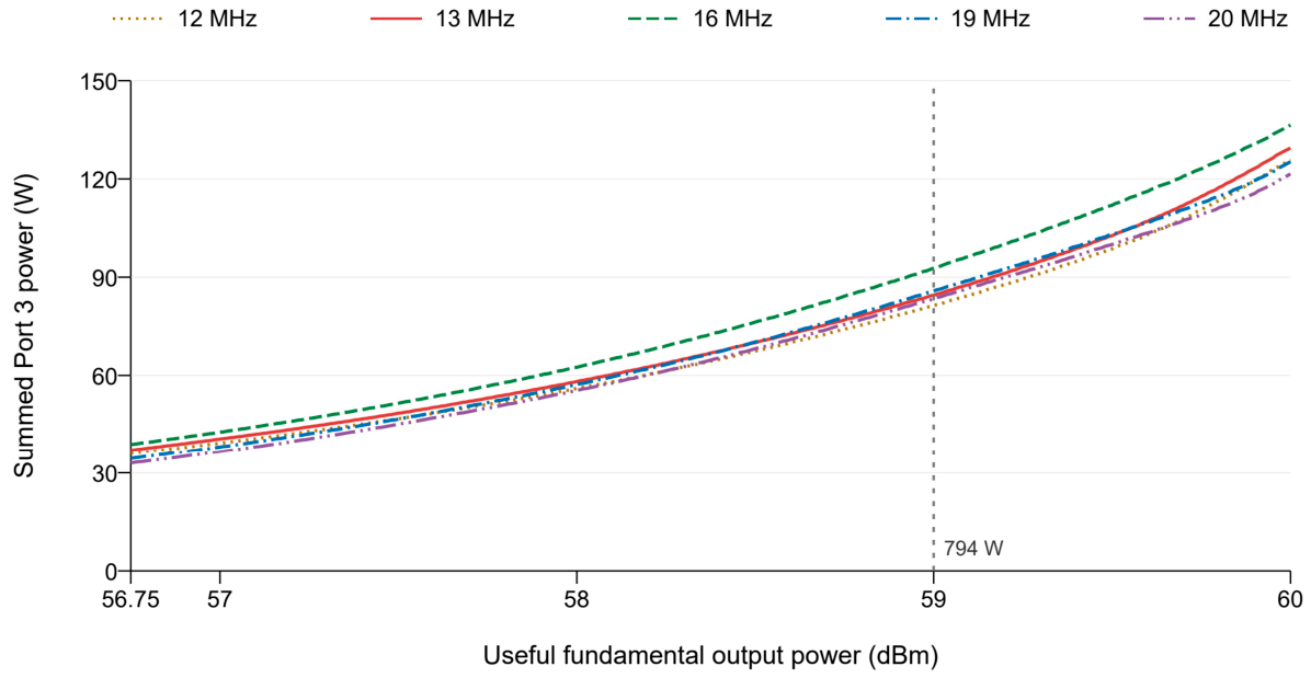
The substituted attenuation path provides direct experimental access to the harmonic-port spectrum. Individual dBm powers were converted to watts before adding carrier leakage and H2–H4. The sum is limited to these recorded components and is not an independent broadband power-meter reading. Figure 9 shows the resulting power scan; Table 8 gives the component powers at the common 794 W useful output.
Figure 9.
Experimental power at Port 3 with the original termination replaced by a 200 W, 40 dB attenuation path. Powers are corrected to the Port 3 input plane. Each curve is the linear sum of measured carrier leakage and H2–H4. The vertical line marks 59 dBm useful output; this test configuration differs from the original-termination output-spectrum and thermal tests.
Table 8.
Attenuation-corrected Port 3 spectral powers at 59 dBm useful fundamental output. Component dBm values are converted to watts before summation; carrier leakage is shown in mW.
At 794 W useful output, the recorded sum is 81.4–92.8 W and is dominated by H3. Carrier leakage is only 0.50–7.60 mW across the five carriers. At 1000 W useful output, the largest recorded sum is 136.5 W at 16 MHz, corresponding to 68.2% of the attenuator’s nominal 200 W rating. This ratio provides a nameplate-loading reference; mounting and thermal derating enter the component assessment in Section 6.3.
These measurements demonstrate high-power transfer of harmonic energy into the Port 3 test path. The recorded spectral sum quantifies delivered power under the substituted load. A transfer fraction additionally requires the incident harmonic power at the filter input. The attenuation path and the original 250 W termination are separate load configurations; their records are therefore kept distinct in the power accounting. Section 6.3 defines the corresponding source, load, and measurement scope.
5.6. System Fundamental-Output Efficiency
System efficiency refers to useful fundamental output divided by the power drawn from the single system DC input:
Here, the numerator is useful fundamental output power in watts, the DC input voltage is 48.2 V, and the system input current is in amperes. The current records are interpolated in useful-output power to 59 dBm for each configuration. The denominator includes all circuitry supplied by that input; no separate final-stage drain efficiency or power-added efficiency is inferred. Table 9 reports the comparison.
Table 9.
System supply current and fundamental-output efficiency at a common 59 dBm useful output, approximately 794 W, with a 48.2 V system supply. Δη is the with-filter value minus the without-filter value in percentage points.
Without the filter, system efficiency is 61.5–62.6%; with the filter, it is 50.7–57.9%. The reduction is 3.7–4.0 percentage points at 12–13 MHz and 10.7–11.2 points at 16–20 MHz. These values quantify the frequency-dependent system-power cost associated with the measured harmonic suppression.
The useful-band filter loss of 0.16–0.20 dB corresponds to approximately 3.6–4.5% fundamental-power loss. At 16 MHz and equal useful output, the additional DC input is 48.2 × (32.434 − 26.809) ≈ 271 W. This system-level change exceeds the contribution expected from the measured passive insertion loss alone. Changed harmonic loading, the drive required for equal output, and the PA operating state are possible contributors. Harmonic suppression and system input current should therefore be assessed together when selecting the operating point. Port 3 power from the substituted-load test is reported separately from useful-output efficiency.
5.7. CW Operation and Recorded Temperatures
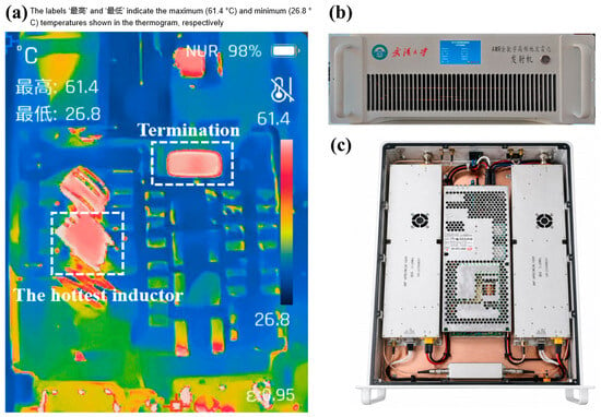
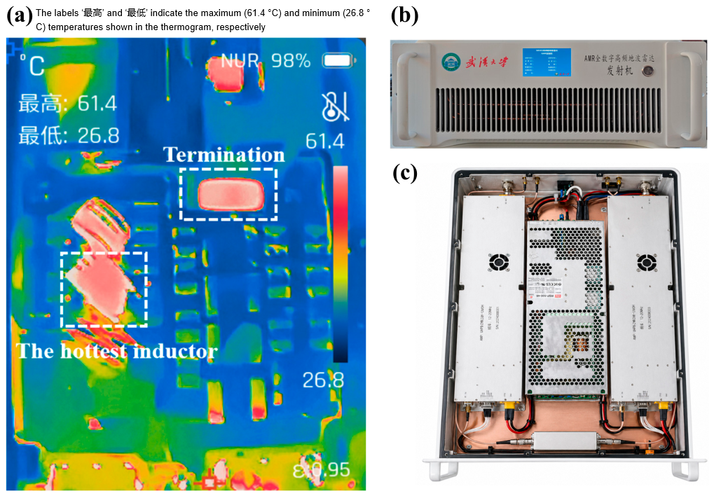
A separate CW test with the original 250 W termination operated at 16 MHz and approximately 794 W for 2 h with the cover removed and module fan switched off. This configuration was maintained during operation and infrared imaging. No arcing, PA protection action, or observable output-power decline occurred. Immediately after the test, a Raythink EX100 with emissivity set to 0.95 recorded a maximum inductor surface temperature of 57.5 °C during live inspection. The saved thermogram in Figure 10a shows 61.4 °C at the termination. At 28.6 °C ambient, the corresponding temperature rises are 28.9 °C and 32.8 °C. These are the recorded two-hour endpoint temperatures. Normal product operation uses the cover and fan; the thermal scope is discussed in Section 6.3.
Figure 10.
(a) Thermogram immediately after the 2 h CW test at 16 MHz and 794 W (cover removed, fan off, emissivity 0.95), showing 61.4 °C at the termination. (b) Transmitter exterior. (c) Internal product assembly. The filter and its PA-module integration are shown in Figure 6.
The filter has been incorporated into ocean radar products, and more than 20 filter units have been installed. Figure 10b,c show the transmitter exterior and internal assembly; the filter and its PA-module integration are shown in Figure 6. Operational observations from the installed products indicate stable filter operation. This product experience complements the controlled laboratory characterization.
6. Discussion
6.1. Contribution in Relation to Prior Work
The contribution is a practical co-design and tuning procedure for high-order lumped LC branches under high-power component constraints. Reference [9] provides basic two- to six-pole absorptive designs, resonant traps, and kilowatt operation. Reference [13] experimentally demonstrates second- and third-order absorptive prototypes and tabulates designs through the fifth order. Reference [18] uses thirteenth-order distributed prototypes with joint full-wave design. The present network combines nominal ninth-order LP and seventh-order HP branches with fourteen selected RF capacitors and seven adjustable coils. Its implementation challenge is quantified by the 5.5 dB rejection degradation caused by a −1% LP2 change, and addressed through joint inductance refinement and response-specific adjustment guidance. The prototype then demonstrates 47.1 dB minimum small-signal rejection and 58.2–66.0 dB H3 improvement at 794 W, with product integration documented in Section 5.7.
Table 10 compares branch order, realization, tuning approach, and measured performance. Frequency bands and test configurations retain the conditions of each source. Small-signal rejection and PA harmonic improvement are separate metrics. NR identifies a quantity not reported in a directly comparable form; N/A identifies a separate port not exposed by that architecture.
Table 10.
Comparison of filter order, implementation, and measured performance with representative absorptive filters and a diplexer [9,13,18]. Frequency bands, port definitions, and test configurations retain the conditions of each source.
6.2. Design Implications Under Component Constraints
Separating capacitor selection from coil refinement makes the high-order network realizable with available RF parts. The V2-to-V3 comparison holds topology, fourteen capacitors, and loss models fixed, isolating the 11.8 dB improvement obtained by jointly adjusting the seven inductances. The selected design exchanges 3.3 percentage points of minimum T3 and some matching performance for this rejection gain (Table 4). The comparisons in Section 2.4 quantify the effect of changing rejection weights and search bounds. These results provide a basis for choosing the rejection–routing compromise according to the intended PA operating conditions.
The connected network should next be assessed in the useful band, harmonic band, and transition. The common-junction diagnostic in Section 2.2 identifies loading that isolated branch transmission can conceal. Evaluating R, T2, and T3 together then shows where rejected power goes. For example, at 80 MHz the measured 32.6% reflection explains most of the reduction in T3, even though Port 2 retains deep rejection. This distinction makes harmonic loading a separate design consideration from output spectral suppression.
The high-order response also requires coordinated physical tuning. LP2 changes of −1% and +1% reduce minimum rejection by 5.5 and 1.3 dB, respectively, so the response to each direction is more useful than the central slope alone for preserving the nominal rejection. LP3/LP4 and HP1/HP2 provide corresponding adjustment priorities for useful-band matching and harmonic routing (Table 5). Physical changes in turn spacing also affect coupling and self-capacitance, making a complete-network VNA check part of the adjustment procedure. The simulated perturbations supply local tuning guidance for the V3 neighborhood.
6.3. Measurement Scope and Design Extensions
Small-signal results establish transmission, port reflection, and frequency-dependent power fractions with 50 Ω terminations. The measured 80 MHz values, T3 = 65.3% and R = 32.6%, identify upper-band harmonic matching as a refinement priority. The prescribed Q values and 200 kHz coil readings support the nominal model and preliminary adjustment. A broadband model would additionally require measured coil Q, self-resonance, and assembly coupling. The numerical scenarios in Section 5.3 assess these mechanisms independently; their parameters are illustrative rather than extracted from the prototype.
High-power characterization comprises five-carrier output harmonics and Port 3 spectral power under the 200 W, 40 dB substituted-load condition. Incident and reflected harmonic waves at the filter input were not recorded, so high-power transfer and absorption fractions remain to be measured. The substituted path and original 250 W termination can present different harmonic impedances. PA source impedance, load-mismatch response, and formal stability over the operating envelope are further system-characterization tasks. The 11.4 dB H2 improvement discrepancy at 13 MHz likewise calls for measurements separating drive and harmonic-load effects.
The single 48.2 V input defines system fundamental-output efficiency, including all circuitry supplied by that input; separate final-stage drain efficiency and power-added efficiency were not measured. The weakest useful-output harmonic is 7.3 dB above the recorded analyzer background. A full uncertainty budget would combine attenuation calibration, detector response, and noise contributions.
The thermal result is the two-hour endpoint at 16 MHz and 794 W with the original termination, cover removed, and fan off. Temperature histories and tests over additional power and cooling conditions are needed to establish equilibrium and lifetime behavior. The carrier-only stress estimates in Section 5.1 support component assessment; complete RF margins require the selected part ratings, harmonic excitation, and thermal derating. Extension to other bands or powers should reassess component impedances, coupling, load matching, and cooling.
7. Conclusions
A high-order quasi-absorptive HF harmonic filter has been realized through component-constrained co-design. Its nominal ninth-order LP and seventh-order HP branches use fourteen selected capacitors and seven adjustable air-core inductors. Joint refinement increases minimum simulated rejection from 37.5 to 49.3 dB while minimum harmonic-port transfer changes from 86.6% to 83.3%. Two-sided perturbations identify coil-specific tuning priorities.
The prototype achieves 0.16–0.20 dB measured insertion loss and 47.1 dB minimum rejection. At 794 W useful output, five-carrier measurements demonstrate 58.2–66.0 dB H3 improvement. The separate Port 3 path records 81.4–92.8 W summed carrier and H2–H4 power at that output, reaching 136.5 W during the scan. System efficiency is 50.7–57.9% with the filter and 61.5–62.6% without it. The original termination reaches 61.4 °C at the two-hour, 16 MHz, 794 W endpoint. More than 20 filter units have been installed in ocean radar products, with stable operation observed in product use.
The measured upper-band mismatch identifies harmonic-port matching as the next design priority. The high-order LC implementation and quantified tuning procedure provide a practical reference for HF PA output networks built from available RF components. Section 6.3 specifies the measurement scope and further characterization tasks.
Author Contributions
Conceptualization, X.W.; methodology and circuit simulation, L.Y.; prototype fabrication, L.Y. and X.X.; writing—review and editing (language), L.Z. All authors have read and agreed to the published version of the manuscript.
Funding
This research was funded by the Southern Marine Science and Engineering Guangdong Laboratory (Zhuhai), grant number SML2024SP016.
Data Availability Statement
The measurement data, simulation files, and optimization and sensitivity-analysis materials supporting the findings of this study are available from the corresponding author upon reasonable request.
Conflicts of Interest
The authors declare no conflicts of interest.
Abbreviations
The following abbreviations are used in this manuscript:
| ADS | Advanced design system |
| CW | Continuous wave |
| DC | Direct current |
| HF | High frequency |
| HP | High pass |
| IF | Intermediate frequency |
| LCR | Inductance–capacitance–resistance |
| LP | Low pass |
| MIMO | Multiple-input multiple-output |
| PA | Power amplifier |
| RBW | Resolution bandwidth |
| RF | Radio frequency |
| rms | Root mean square |
| TRM | Through–reflect–match |
| VNA | Vector network analyzer |
| VSWR | Voltage standing wave ratio |
References
- Trizna, D.; Xu, L. Target classification and remote sensing of ocean current shear using a dual-use multifrequency HF radar. IEEE J. Ocean. Eng. 2006, 31, 904–918. [Google Scholar] [CrossRef] [Scilit]
- Yang, J.; Wang, R.; Shi, Y.; Xu, X.; Li, S.; Wang, C.; Zhou, H.; Wen, B.; Wu, S. Dual-use multistatic HF ocean radar for current mapping and ship tracking. IEICE Electron. Express 2014, 11, 20140281. [Google Scholar] [CrossRef] [Scilit]
- Mantovani, C.; Corgnati, L.; Horstmann, J.; Rubio, A.; Reyes, E.; Quentin, C.; Cosoli, S.; Asensio, J.L.; Mader, J.; Griffa, A. Best practices on high frequency radar deployment and operation for ocean current measurement. Front. Mar. Sci. 2020, 7, 210. [Google Scholar] [CrossRef] [Scilit]
- Xie, X.; Zhang, L.; Chen, Z.; Wu, X.; Yue, X. MIMO ground wave radar radio frequency monitoring. IEEE Geosci. Remote Sens. Lett. 2022, 19, 4025405. [Google Scholar] [CrossRef] [Scilit]
- Wang, M.; Wu, X.; Zhang, L.; Yue, X.; Yi, X.; Xie, X.; Yu, L. Measurement and analysis of antenna pattern for MIMO HF surface wave radar. IEEE Antennas Wirel. Propag. Lett. 2023, 22, 1788–1792. [Google Scholar] [CrossRef] [Scilit]
- Mo, F.; Wu, X.; Li, X.; Yu, L.; Zhou, H. A directional wave spectrum inversion algorithm with HF surface wave radar network. Remote Sens. 2025, 17, 2573. [Google Scholar] [CrossRef] [Scilit]
- Cripps, S.C. RF Power Amplifiers for Wireless Communications, 2nd ed.; Artech House: Norwood, MA, USA, 2006. [Google Scholar]
- Cohn, S.B.; Coale, F.S. Directional channel-separation filters. Proc. IRE 1956, 44, 1018–1024. [Google Scholar] [CrossRef] [Scilit]
- Weinreich, R.; Carroll, R.W. Absorptive filter for TV harmonics: And a novel filter construction technique. QST 1968, 52, 20–25. [Google Scholar]
- Morgan, M.A.; Boyd, T.A. Theoretical and experimental study of a new class of reflectionless filter. IEEE Trans. Microw. Theory Techn. 2011, 59, 1214–1221. [Google Scholar] [CrossRef] [Scilit]
- Morgan, M.A.; Boyd, T.A. Reflectionless filter structures. IEEE Trans. Microw. Theory Techn. 2015, 63, 1263–1271. [Google Scholar] [CrossRef] [Scilit]
- Morgan, M.A.; Groves, W.M.; Boyd, T.A. Reflectionless filter topologies supporting arbitrary low-pass ladder prototypes. IEEE Trans. Circuits Syst. I Regul. Pap. 2019, 66, 594–604. [Google Scholar] [CrossRef] [Scilit]
- Lee, T.-H.; Lee, B.; Kim, Y.-S.; Wu, K.; Lee, J. Higher order lumped element absorptive low-pass and bandpass filter structures. IET Microw. Antennas Propag. 2019, 13, 1166–1173. [Google Scholar] [CrossRef] [Scilit]
- Yang, L.; Gomez-Garcia, R.; Munoz-Ferreras, J.-M.; Zhang, R. Input-reflectionless low-pass filter on multilayered diplexer-based topology. IEEE Microw. Wirel. Compon. Lett. 2020, 30, 945–948. [Google Scholar] [CrossRef] [Scilit]
- Jin, X.-H.; Huang, X.-D.; Ren, Q.; Cheng, C.-H. Four-port symmetrical reflectionless lumped filter/diplexer: Prototype and design table. IEEE Trans. Microw. Theory Techn. 2021, 69, 2211–2219. [Google Scholar] [CrossRef] [Scilit]
- Zhang, A.; Xu, J.; Liu, Z.; Zhang, Y. Microstrip quasi-elliptic absorptive bandpass filter with ultra-wide reflectionless range and compact size. Electronics 2024, 13, 1841. [Google Scholar] [CrossRef] [Scilit]
- Zhu, Y.-H.; Fang, X.-Y.; Xie, X.; Yang, L.-L.; Chen, J.-X. Design of a two-port reflectionless waveguide bandpass filter with high power handling capability. AEU—Int. J. Electron. Commun. 2024, 176, 155158. [Google Scholar] [CrossRef] [Scilit]
- Miri, S.-M.; Mohammadpour-Aghdam, K.; Miri, S.-O. A wideband, sharp roll-off U-band diplexer in suspended stripline technology. Int. J. RF Microw. Comput.-Aided Eng. 2023, 2023, 9872407. [Google Scholar] [CrossRef] [Scilit]
- Rhea, R.W. Exploiting filter symmetry. Microw. J 2001, 44, 100–108. Available online: https://www.microwavejournal.com/articles/3162-exploiting-filter-symmetry (accessed on 7 September 2026).
- Bandler, J.W.; Chen, S.H.; Daijavad, S. Exact sensitivity analysis for optimization of multi-coupled cavity filters. Int. J. Circuit Theory Appl. 1986, 14, 63–77. [Google Scholar] [CrossRef] [Scilit]
- SciPy Community. Scipy.optimize.least_squares. SciPy Reference Guide. Available online: https://docs.scipy.org/doc/scipy/reference/generated/scipy.optimize.least_squares.html (accessed on 7 September 2026).
- Keysight Technologies. Introduction to Circuit Components; Advanced Design System 2016.01; 2016; INDQ Component. pp. 208–209. Available online: https://edadownload.software.keysight.com/eedl/ads/2016_01/pdf/Introduction_to_Circuit_Components.pdf (accessed on 7 September 2026).
- Agilent Technologies. Introduction to Circuit Components; Advanced Design System 2011.01; 2011; CAPQ Component. Available online: https://edadownload.software.keysight.com/eedl/ads/2011_01/pdf/ccsim.pdf (accessed on 7 September 2026).

Disclaimer/Publisher’s Note: The statements, opinions and data contained in all publications are solely those of the individual author(s) and contributor(s) and not of MDPI and/or the editor(s). MDPI and/or the editor(s) disclaim responsibility for any injury to people or property resulting from any ideas, methods, instructions or products referred to in the content. |
© 2026 by the authors. Licensee MDPI, Basel, Switzerland. This article is an open access article distributed under the terms and conditions of the Creative Commons Attribution (CC BY) license.