


Abstract
This study adapts RT-DETR for two-dimensional bounding-box localization of upper and lower structural connection regions on transmission towers. The architecture combines a C2f_SHSA_CGLU backbone, deformable encoder attention, and SBA_fused with a high-resolution P2 level. The private dataset contains 818 images and 12,541 boxes. The 655-image training split is paired with a 163-image validation split used for both checkpoint selection and performance reporting. There is no independent test partition for the private task. On this validation split, our seed 0 achieves an AP of 59.14% and a small-object AP of 52.06%, compared with 56.68% and 44.88% for RT-DETR-r18. The backbone controls show no consistent CGLU accuracy benefit. In a separate three-seed ablation, the P2 and SBA_fused configuration achieves an AP of 58.33 ± 0.79%, compared with 55.67 ± 0.69% when both are omitted. On the five-class public STN PLAD benchmark, our model achieves an AP of 37.53 ± 4.51% versus 44.18 ± 1.26% for RT-DETR-r18. The observed gains apply to the private validation setting. Generalization of the private labels to independent scenes remains unverified. The desktop file-input pipeline reaches 14.94 FPS on an NVIDIA GeForce RTX 3090 (NVIDIA Corporation, Santa Clara, CA, USA).
1. Introduction
Integrated satellite–terrestrial networks provide communication and remote-sensing support for next-generation smart-grid operation [1]. Within transmission infrastructure inspection, deep-learning detectors have been investigated for insulator defects in drone images [2] and foreign objects on transmission lines in UAV images [3]. UAV imagery provides flexible and comprehensive visual information for inspection, while automated visual interpretation and structural-region localization remain critical front-end components. Recent comprehensive reviews summarize UAV sensing technologies, computer-vision algorithms, and operational constraints encountered in power-line and transmission tower inspection [4]. In an adjacent remote-sensing task, CalFireSegNet combines attention and transformer components for post-wildfire building-footprint change analysis [5]; this provides a methodological context rather than a direct tower-detection benchmark. The present study focuses on 2D image-space localization of transmission tower structural connection regions to guide motorized optical distance-measurement instruments.
Images of transmission infrastructure can support automated inspection and geometric analysis. This study focuses on locating annotated structural features on towers, including features assigned to upper and lower regions. Such locations may serve as inputs to a subsequent coordinate-estimation pipeline. The detection problem is evaluated in image space; three-dimensional reconstruction additionally requires a defined correspondence and camera/geometric procedure and is not established by detection AP alone.
Recent journal studies distinguish several levels of visual inspection. Cheng et al. [6] combine semantic and boundary information to detect complete towers in remote-sensing images. Bellou et al. [7] evaluate YOLOv8 for towers, insulators and conductors in aerial and ground imagery. Wang and Wang [8] separately detect the tower top, crossarm, insulator, tower body and tower base, then use detection-box centers in a navigation-information estimator. Their component localization is particularly relevant to the present image-space task, although their classes, distribution-tower setting and route-generation objective differ from our two upper/lower structural-region classes and intended rangefinder alignment. Zhang et al. [9] study multi-scale component detection on InsPLAD, with feature interaction and confidence refinement. These studies provide related task and method context; differences in data, label granularity and evaluation prevent direct ranking of their published scores against ours. Table 1 summarizes these studies and the scope of the present task.
Table 1.
Related journal studies and the scope of the present structural-region task. This is a task comparison, not a cross-dataset accuracy ranking.
Two-stage CNN detectors use region proposals and shared features, as developed in R-CNN [10], Fast R-CNN [11] and Faster R-CNN [12]; Mask R-CNN [13] further adds instance segmentation. These designs establish general detection principles but do not define the structural-region labels evaluated here.
One-stage detectors predict categories and boxes from feature maps. YOLO [14], YOLOv10 [15] and YOLOv12 [16] investigate accuracy and efficiency trade-offs, while SSD [17] uses multi-scale feature maps and RetinaNet [18] addresses class imbalance through focal loss. These general methods motivate the choice of comparators; they do not by themselves establish performance on the present task.
Transformer-based detectors provide a compelling alternative to conventional CNN architectures by formulating object detection as a direct set prediction. DETR [19] eliminates handcrafted anchors and non-maximum suppression, while deformable DETR [20] incorporates multi-scale deformable attention to accelerate training convergence and feature processing. More recently, RT-DETR [21] developed an efficient hybrid encoder and an uncertainty-minimal query selection strategy to achieve a favorable accuracy–throughput trade-off on real-time benchmarks. Its hybrid architecture decouples intra-scale self-attention from cross-scale feature fusion. The present work adapts and optimizes this framework for the fine-grained transmission tower structural localization task described in Section 2.
Structural feature localization in complex tower images presents two challenges addressed by this architecture: confusion with background or nearby structure, and loss of detail in small annotated feature regions.
Background interference: Metal lattice patterns, vegetation, cables and building edges may resemble annotated tower features. Similar visual patterns can produce false detections or category confusion. The proposed contextual processing is motivated by this difficulty; its effect requires a held-out error analysis.
Small feature regions: One tower may occupy a substantial part of the image while each annotated feature region covers few pixels. Downsampling can remove detail in these local regions. This task must therefore distinguish small annotated features from small or distant complete towers. Its size-specific evaluation uses the confirmed local annotation geometry.
We adapt RT-DETR to the annotated structural-feature localization task, using contextual feature processing, deformable attention and multi-scale fusion. The contributions are defined as the following integration choices and will be evaluated with controlled comparisons.
- Integrate established C2f, SHSA and convolutional gating in a YOLOv8-style backbone for the specified structural-region task. The contribution is an implementation and task adaptation, not a new attention or gating mechanism. Four block variants are evaluated over three seeds; the composite reduces parameters relative to plain C2f, but does not show a consistent accuracy advantage over the alternatives.
- Adapt the RT-DETR encoder using existing deformable attention to permit content-dependent feature sampling. The historical grouped ablation is retained without inferring that every component combination improves performance or reduces computation.
- Integrate SBA_fused and a high-resolution P2 level and evaluate four fusion configurations over three seeds. The joint configuration yields the highest AP on the fixed private validation split, with an increase in parameters. The supplementary five-class STN PLAD benchmark tests performance on a different label set and identifies a setting where the full architecture trails RT-DETR-r18.
2. Dataset Construction
A comprehensive audit of our archived records confirmed that the benchmark dataset consists of 818 high-resolution aerial and ground-based images containing 12,541 precisely annotated target instances. The images were captured across diverse urban and rural operational environments, encompassing varied background clutter (dense forests, farmlands, and complex terrains) and illumination conditions (strong backlighting and overcast daylight). The original images feature high resolutions, including 3000 × 4000 (331 images), 1920 × 1080 (190 images), 5472 × 3648 (140 images), and 3000 × 3000 (126 images) pixels. The historical mention of 6000 images in preliminary records reflected uncurated raw field video frames and collection logs; all experiments reported herein are strictly and reproducibly bound to the audited 818-image benchmark.
2.1. Task Formulation and Annotation Semantics
In contrast to conventional object detection frameworks that enclose an entire transmission tower within a single coarse bounding box, this work formulates the problem as fine-grained structural-region localization. Specifically, the detector identifies critical upper and lower structural connection zones and outputs 2D bounding boxes whose centroids guide motorized pan-tilt units in aiming optical distance-measurement instruments. It should be emphasized that the scope of this study is strictly confined to evaluating the 2D visual localization accuracy, precision–recall trade-offs, and computational efficiency of this front-end perception module; downstream 3D coordinate triangulation constitutes a subsequent system-level integration step rather than an end-to-end task validated herein.
Using the X-AnyLabeling annotation suite (https://github.com/CVHub520/X-AnyLabeling, accessed on 11 November 2026), target regions were delineated with normalized 2D bounding boxes and categorized into two structurally distinct semantic classes: (1) Class 0 (dian), which denotes structural connection regions situated strictly below the tower crossarm, primarily encompassing lower lattice braces, post-connection gussets, and leg junctions (7874 total instances: 6284 training and 1590 validation); and (2) Class 1 (dian1), which denotes structural connection regions located at and above the tower crossarm, comprising crossarm truss joints, wire-hanging points, and tower crest structures (4667 total instances: 3753 training and 914 validation).
2.2. Dataset Splitting and Scale Distribution
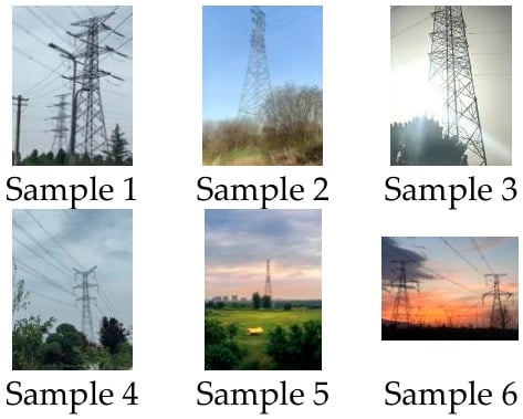
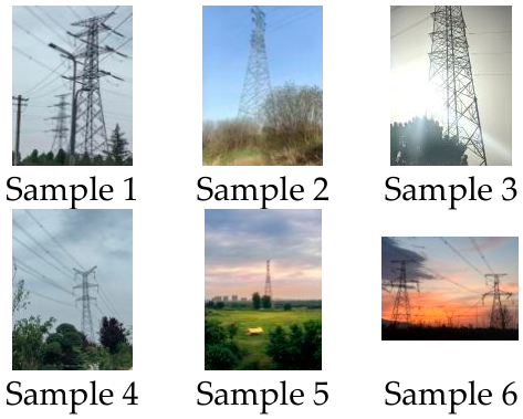
A rigorous audit of our archival collection records verified that the curated benchmark dataset consists of 818 high-resolution aerial and ground-based keyframes containing 12,541 annotated target instances. These keyframes were acquired across diverse urban and rural operational environments, spanning complex background clutter (such as dense forests, farmlands, and rugged terrain) as well as challenging illumination conditions (including severe backlighting and overcast daylight). The native imagery encompasses multiple high-resolution formats, specifically 3000 × 4000 (331 images), 1920 × 1080 (190 images), 5472 × 3648 (140 images), and 3000 × 3000 (126 images) pixels. Whereas preliminary documentation referenced approximately 6000 images—a figure reflecting raw, uncurated field video frames and acquisition logs—all experimental results reported in this manuscript are strictly and reproducibly bound to the audited 818-image benchmark. The dataset is partitioned into training and validation subsets following an approximate 80:20 split: 655 images (80.07%, containing 10,037 target instances) are allocated for model training, and 163 images (19.93%, containing 2504 target instances) are reserved for validation and model selection. Evaluated under standard COCO scale definitions based on bounding box pixel area in native image coordinates—small (<322 px), medium (322–962 px), and large (≥962 px)—the annotated instances exhibit pronounced multi-scale diversity. Specifically, small-scale targets account for 27.4% of the dataset (3436 instances: 2798 training and 638 validation), medium-scale targets represent 51.67% (6480 instances: 5170 training and 1310 validation), and large-scale targets constitute the remaining 20.93% (2625 instances: 2069 training and 556 validation). Figure 1 shows representative images from the dataset.
Figure 1.
Representative dataset images.
2.3. Supplementary Public Dataset
STN PLAD [22] contains 133 high-resolution images and 2409 instances in five asset classes: tower, insulator, spacer, damper and plate. We use fixed lists of 85 training, 21 validation and 25 test images, with two buffer images excluded. The test set contains 582 instances: 73 towers, 61 insulators, 49 spacers, 381 dampers and 18 plates; the small/medium/large counts are 60/334/188 in original-image coordinates. The test images come from the dataset directory group 20181129-R, while training and validation images come from 20181127-A1. These source-directory groups do not establish distinct physical towers or fully independent acquisition sequences. This supplementary five-class detection task does not relabel assets as dian/dian1 and cannot directly test transfer of our private structural-region labels.
3. Methodology
3.1. Introduction to Rt-Detr
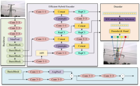
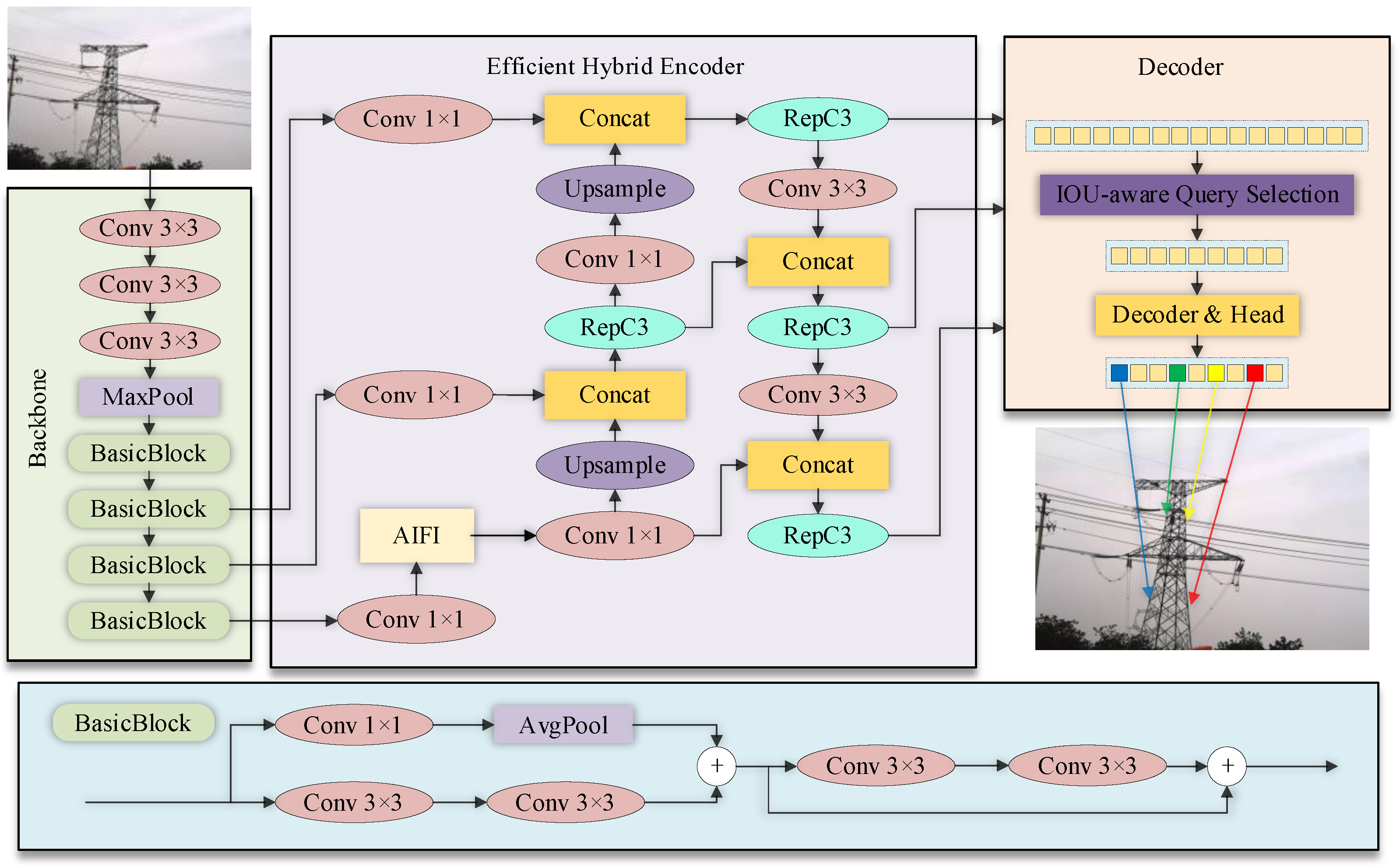
DETR formulates object detection as end-to-end set prediction and removes the need for anchor design and non-maximum suppression in its standard inference pipeline. RT-DETR [21] develops an efficient hybrid encoder and query selection strategy to improve the accuracy–throughput trade-off. Figure 2 summarizes its architecture. This study adapts the framework to the annotation task defined in Section 2.
Figure 2.
Architecture diagram of the RT-DETR model The RT-DETR architecture establishes real-time end-to-end detection via two core components: an efficient hybrid encoder that decouples intra-scale self-attention from cross-scale feature concatenation, and an uncertainty-minimal query selection mechanism [21].
The efficient hybrid encoder aims to solve the problem of excessive computational overhead caused by global self-attention mechanisms when traditional DETR encoders process multi-scale features. This encoder significantly improves efficiency by decoupling intra-scale feature interactions and cross-scale feature fusion. Specifically, the Attention-based Intrascale Feature Interaction (AIFI) module efficiently captures long-range dependencies and rich contextual information within a single feature scale using a self-attention mechanism, avoiding the heavy computational burden of global attention. Subsequently, a lightweight CNN-based Cross-scale Feature-fusion Module (CCFM) promotes information exchange between multi-scale feature maps through efficient convolutional operations, effectively fusing the multi-scale feature maps processed by AIFI. This fusion is crucial for maintaining high detection accuracy for targets of different sizes in complex scenes.
RT-DETR employs an uncertainty-minimal query selection scheme to initialize decoder object queries directly from high-level encoder representations [21]. By explicitly modeling feature uncertainty across classification and localization branches, this mechanism prioritizes high-confidence structural candidate regions and accelerates decoder convergence compared to the static learned queries in early DETR models.
The hybrid encoder combines interactions within a feature scale with fusion across scales. Query selection provides initial features for the decoder. These components establish the framework used in this study; comparisons depend on the specific backbone, implementation, training protocol, and evaluation setting.
3.2. Improved Rt-Detr Model
The target task is localization of upper and lower structural features on towers. Background patterns can produce false detections, and small local regions can lose detail after downsampling. These issues concern annotated feature regions, including those on towers that are large in the image; they should not be interpreted as whole-tower detection results.
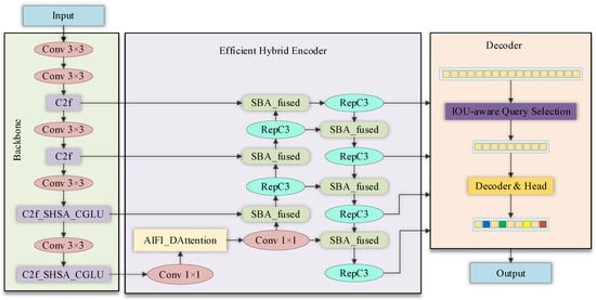
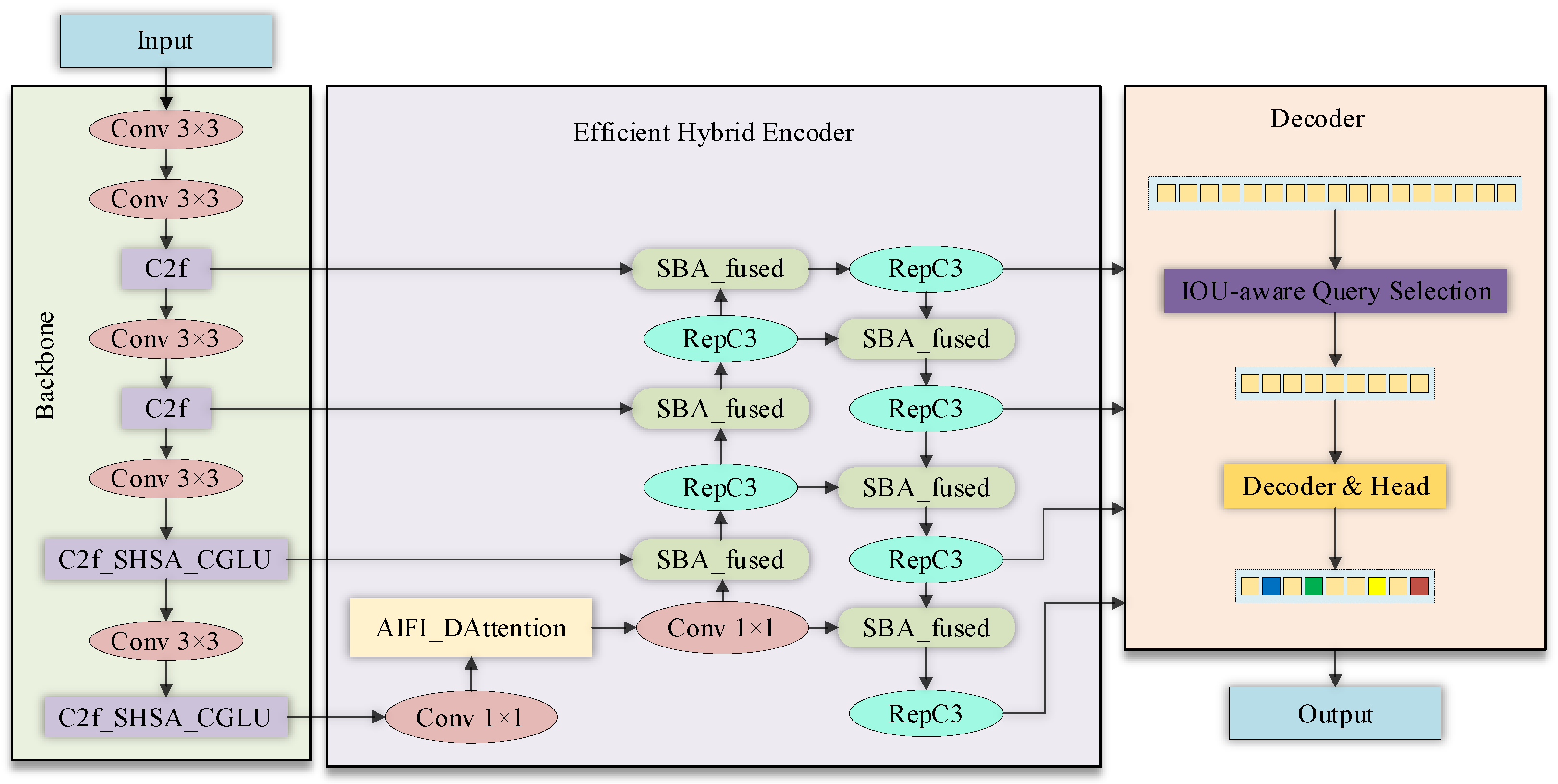
The three architectural adaptations in Figure 3 are intended to improve feature extraction and multi-scale processing for this local structural-feature task. Their effects are evaluated relative to the specified controls.
Figure 3.
Architecture diagram of the improved RT-DETR model.
3.2.1. Backbone Design and Implementation
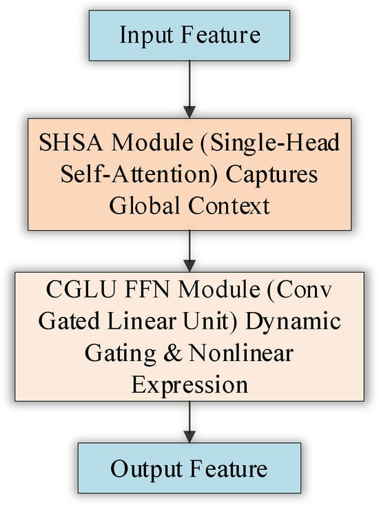
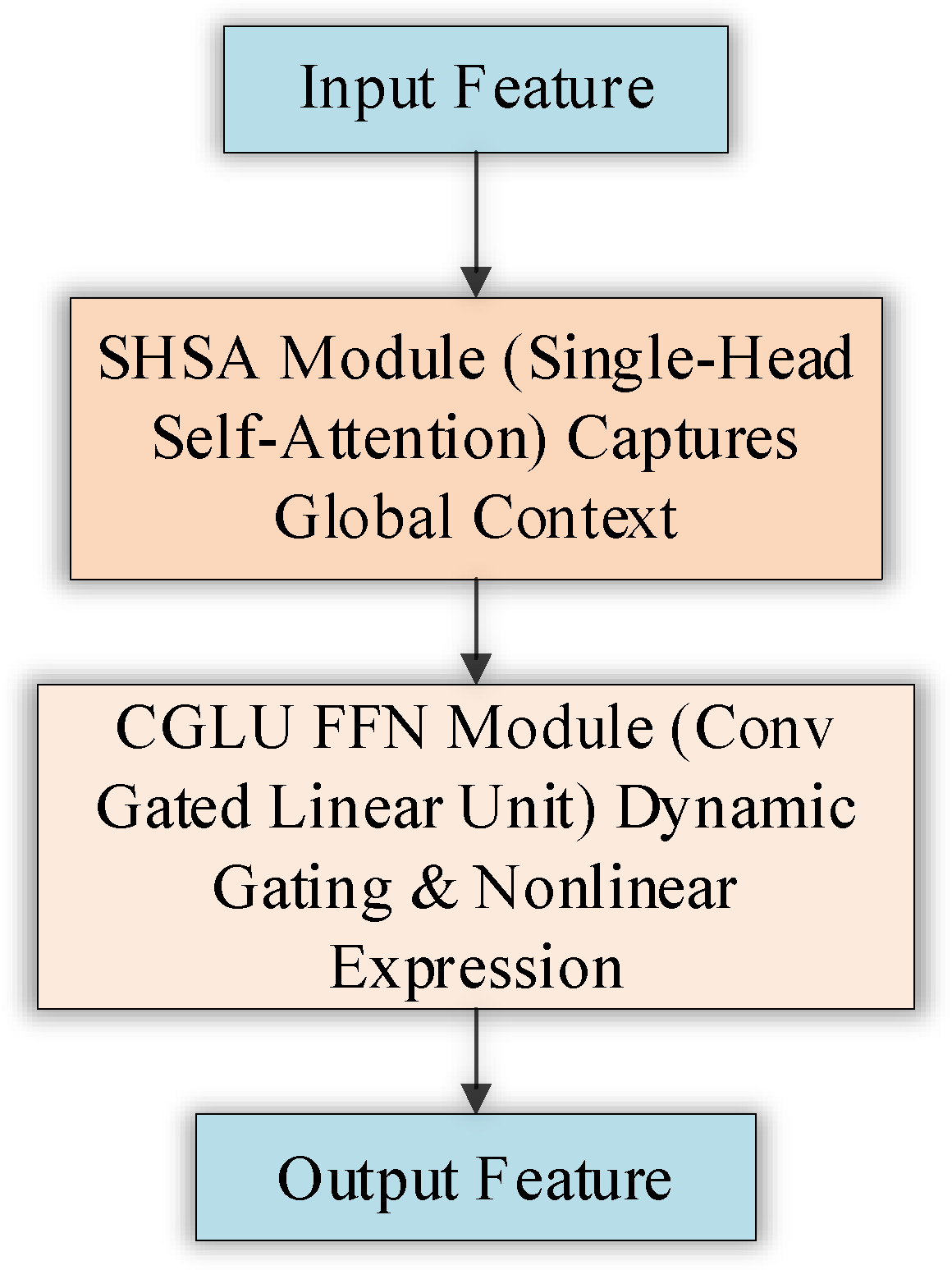
We use a YOLOv8-style backbone as the feature extractor for RT-DETR. Its C2f modules at the selected deeper stages, reported as layers 6 and 8 in the submitted configuration, are replaced by C2f_SHSA_CGLU. This composite module combines C2f, single-head self-attention, and convolutional gating. Figure 4 shows the integration. Changing the backbone and its internal blocks are distinct interventions, so controlled attribution requires the corresponding plain YOLOv8-style backbone without these replacements.
Figure 4.
C2f_SHSA_CGLU module.
The implementation in PyTorch (version 1.13.1+cu117 for the supplementary experiments) and Ultralytics (https://github.com/ultralytics/ultralytics, accessed on 11 November 2026) replaces deeper C2f blocks at backbone layers 6 and 8. At 640 × 640 input, the full model includes P2–P5 and a decoder hidden dimension of 128 with four input levels. Its historical two-class parameter audit gives approximately 16.62 M parameters versus 20.08 M for RT-DETR-r18 (about 17.26% fewer); changing the number of output classes changes exact counts. The new private block controls use a distinct shared configuration with a three-level P3–P5 decoder, hidden dimension 128, 300 queries, four sampling points per decoder attention head, eight heads and three decoder layers, without P2 or SBA. They isolate block replacements within that configuration rather than the entire full-model design.
The C2f_SHSA_CGLU module organically combines efficient Cross-Stage Partial connections (C2f), lightweight global Single-Head Self-Attention (SHSA) [23], and dynamic Convolutional Gated Linear Units (CGLU) [24].
a. Top-Level Framework: Cross-Stage Partial Connection (C2f)
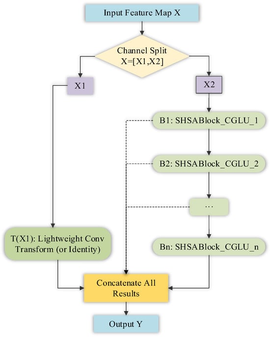
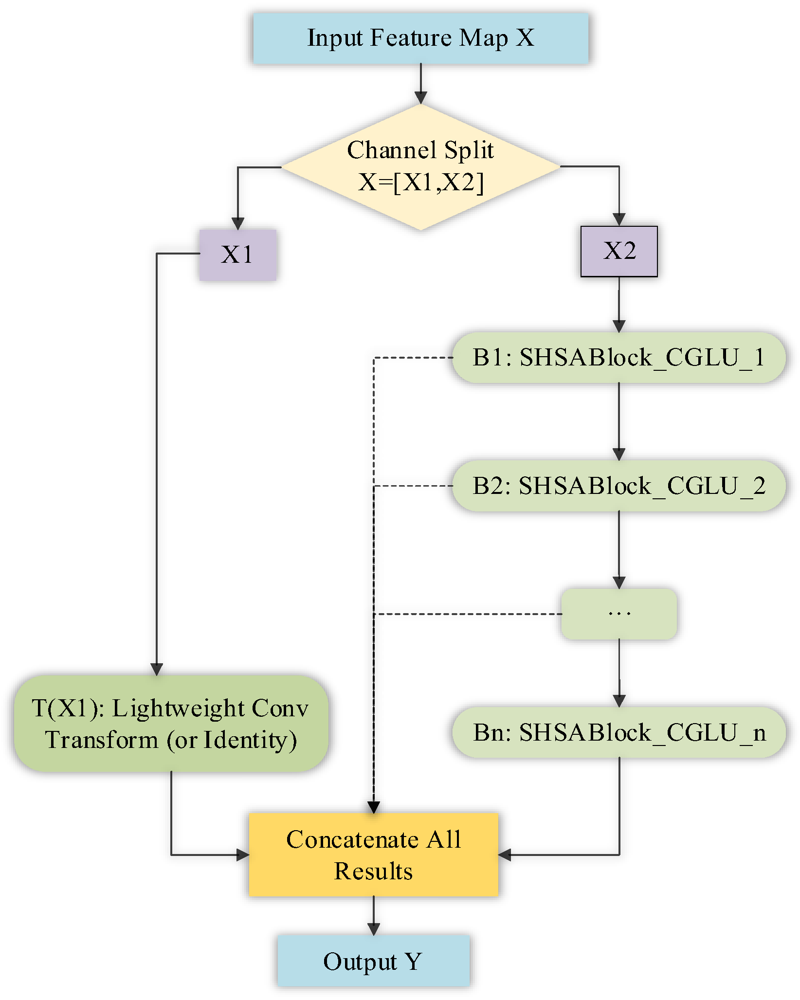
The C2f structure serves as the macroscopic framework of the module, designed to optimize computational resource allocation and enhance gradient propagation. For an input feature map X, C2f first splits it along the channel dimension into two parts: X1 and X2,where X1 ∈ ℝB×(C/2)×H×W and X2 ∈ ℝB×(C/2)×H×W.
Typically, X1 undergoes a single lightweight convolutional transformation (or is directly retained), while X2 is fed into a series of core processing units (i.e., SHSABlock_CGLU) (see Figure 5). Finally, the processing results of the two parts are concatenated. This process can be formulated as:
where (·) represents a shallow transformation of X1, Bi represents the i-th SHSABlock_CGLU core module, and Concat represents the concatenation operation along the channel dimension.
Y = Conv(Concat[(X1),1(2(…(n(X2))))])
Figure 5.
SHSABlock_CGLU Module.
b. Core Unit: Single-Head Self-Attention Mixer (SHSA)
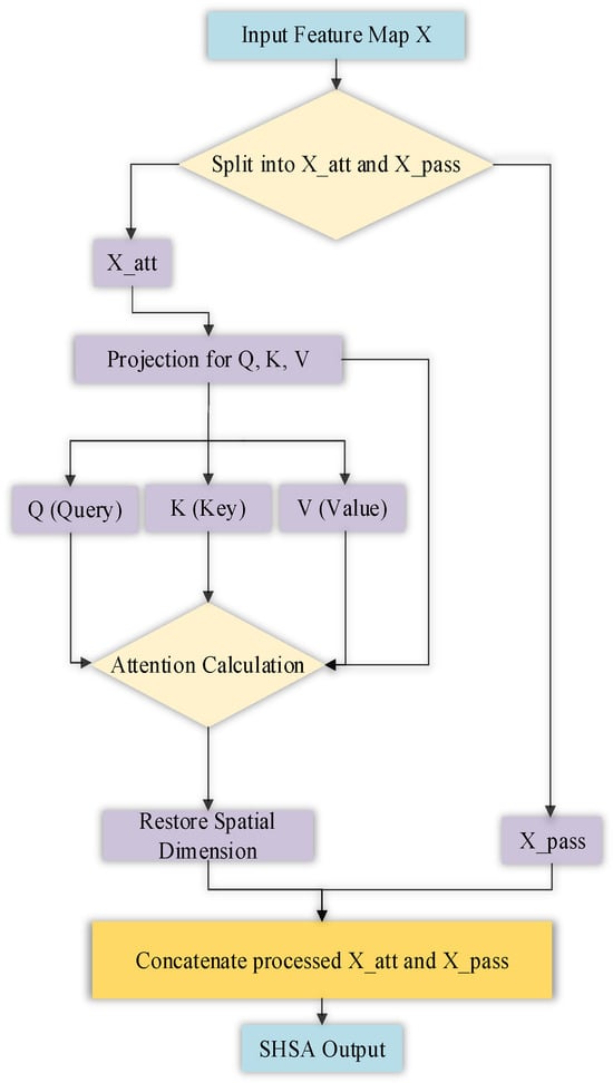
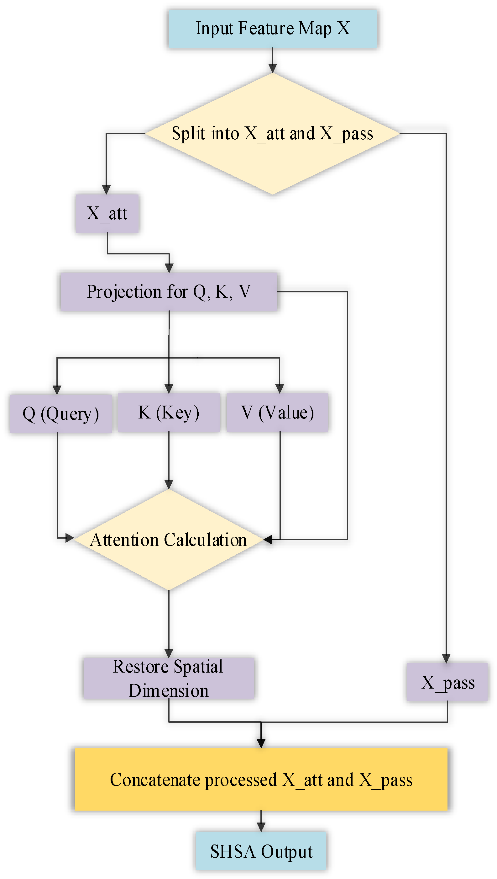
SHSA is a key component within SHSABlock_CGLU used to capture global context; it is a highly optimized self-attention mechanism. Unlike computing attention across all channels, SHSA only performs self-attention operations on a small, fixed subset of channels (dimension d, where d < C/2) of the feature map. The structure diagram of SHSA is shown in Figure 6.
Figure 6.
Architecture of SHSA.
Given an input feature X, SHSA first partitions it into Xatt and Xpass. The self-attention computation is only performed on Xatt:
1. Projection:
where Reshape is a spatial flattening operation, and Wq, Wk, Wv are learnable weight matrices.
2. Attention Score Calculation:
3. Feature Fusion: The result of the attention calculation is restored in the spatial dimension and concatenated with the unprocessed Xpass to form the final output.
c. Convolutional gated linear unit implementation
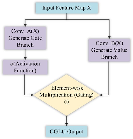
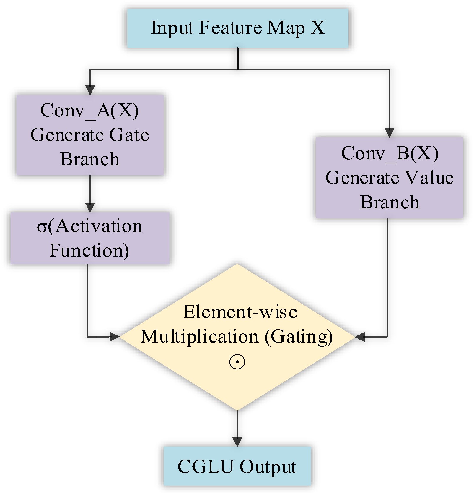
The actual CGLU implementation uses 192 input/output channels inside each modified C2f block. Its constructor receives hidden_features = 384 and computes h = int(2 × 384/3) = 256. A 1 × 1 convolution maps 192 to 512 channels, split into two 256-channel branches. One branch passes through a 3 × 3 depthwise convolution (stride 1, padding 1, groups 256) followed by GELU and is multiplied by the other, unactivated branch. A 1 × 1 convolution projects 256 channels back to 192, with an internal residual connection and dropout probability 0. All three CGLU convolutions use biases. The implementation has no sigmoid gate. Figure 7 illustrates the CGLU branch multiplication.
(u, v) = split(Conv1 × 1(x)); y = x + Conv1 × 1(GELU(DWConv3 × 3(u)) ⊙ v).
Figure 7.
Schematic branch multiplication in CGLU. The implemented convolutions, GELU and residual are specified in Equation (4).
Here u and v each have 256 channels, and ⊙ denotes element-wise multiplication. The enclosing SHSABlock_CGLU first applies a residual 192-channel 3 × 3 depthwise Conv + BN, then residual SHSA (qk_dim = 16, pdim = 64), and finally CGLU. Layer 6 contains one such unit and layer 8 contains three, giving four units in total. The no-SHSA control retains the enclosing depthwise Conv + BN and CGLU, so it is denoted DWConv+CGLU rather than a pure CGLU-only FFN.
The design combines established contextual interaction and multiplicative modulation. Its motivation is architectural; empirical evidence comes from the four-variant repeated control in Section 4.4. Neither the composite form nor the feature-response visualization proves an independent or synergistic accuracy gain.
3.2.2. Improved Aifi Module
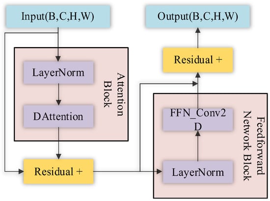
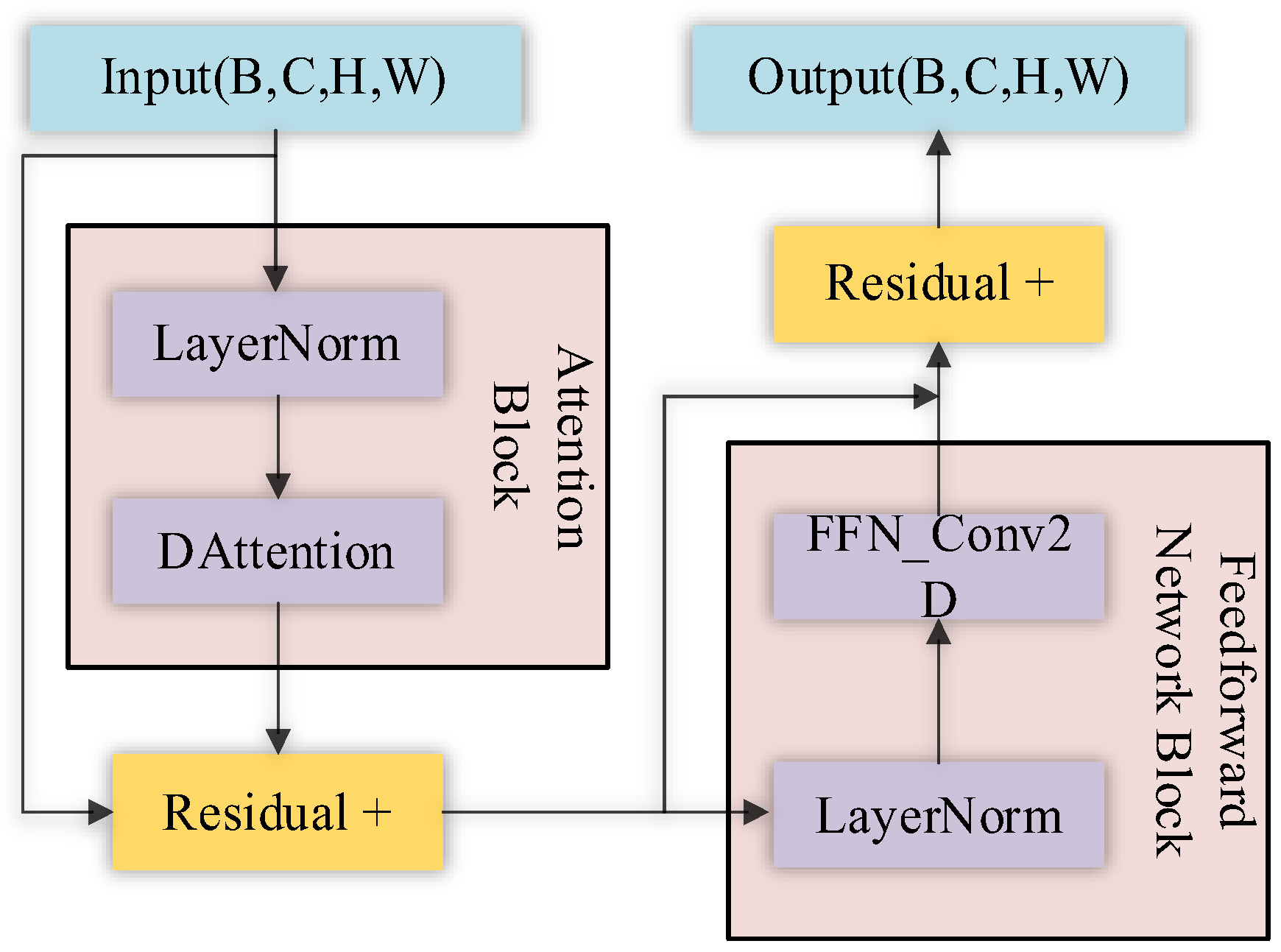
AIFI_DAttention replaces the encoder attention component with deformable attention [25]. Figure 8 shows the adopted block. The implementation determines sampling geometry, sampled-key count, tensor transformations, and computational cost; these details distinguish this adaptation from other deformable-attention formulations.
Figure 8.
Architecture of AIFI_DAttention.
Learned sampling locations allow content-dependent feature selection. Whether this reduces computation depends on sampled positions and the cost of offset generation, projection, and attention.
a. The standard attention term grows quadratically with the number of spatial tokens. The following expression describes this attention term rather than the complete block cost:
ComplexityStandard = O(H2W2C)
If the sampled-key count K is fixed independently of resolution, the attention term is proportional to HWK. This assumption must be checked against the implementation; if the sampled grid grows with H and W, a linear-complexity claim does not follow:
b. Enhanced Focused Feature Learning:
ComplexityDeformable = O(HWCK)
DAttention uses learned offsets to obtain content-dependent key and value features. Heatmaps provide qualitative information, while quantitative ablation and error analysis are required to assess its effect on background interference.
c. Architecture Optimization:
The adopted block uses tensors of shape (B, C, H, W) at its interface. Internal flattening, reshaping, normalization, and interpolation must be reported from the implementation rather than inferred from the interface.
3.2.3. Multi-Scale Feature Fusion Improvement: The Sba_fused Module
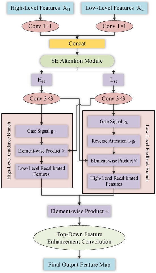
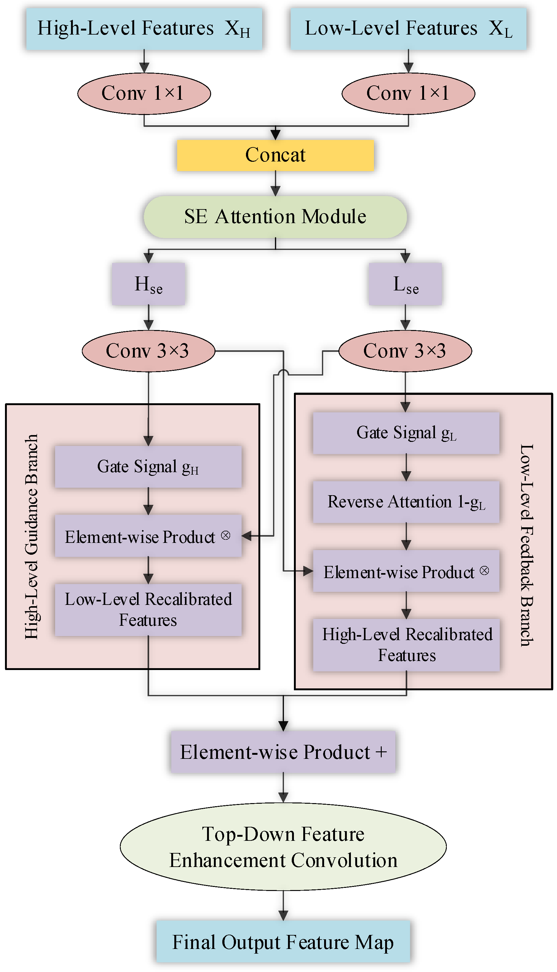
SBA_fused adapts feature fusion in the RT-DETR encoder to exchange information between levels. It combines ideas from Selective Boundary Aggregation (SBA), introduced in DuAT for medical image segmentation [26], contextual processing [27], and SE attention [28]. Figure 9 presents the arrangement. The contribution concerns this fusion arrangement and integration with P2; the underlying mechanisms are credited to prior work.
Figure 9.
Architecture of SBA_fused.
The core idea is that the rich semantic information of high-level features and the fine spatial details of low-level features should guide and refine each other bidirectionally. The processing flow follows these steps:
a. Adaptive Channel Alignment:
1 × 1 convolutional layers adjust the channel numbers of high-level (XH) and low-level features (XL) to a unified dimension:
b. SE Attention Enhancement:
The aligned features are concatenated and passed through a Squeeze-and-Excitation (SE) module [28] to adaptively learn channel importance:
The processed feature is then re-separated into Hse and Lse.
c. Bidirectional Feature Recalibration:
gH = σ(Conv3×3(Hse)), gL = σ(Conv3×3(Lse))
Top-down and bottom-up interactions are intended to preserve local spatial detail while exchanging semantic context. Their actual contribution must be assessed from controlled comparisons rather than inferred from the fusion equations.
d. Context Enhancement and Final Fusion:
The two features are fused via element-wise addition and undergo an additional convolutional layer for contextual representation.
In the SBA_fused module, multi-scale feature maps from levels P2, P3, P4, and P5 (with spatial dimensions of 160 × 160, 80 × 80, 40 × 40, and 20 × 20 at 640 × 640 input resolution) are harmonized through 1 × 1 convolutions to a uniform channel dimension of 128. Spatial alignment is performed using bilinear interpolation for upsampling and strided convolutions for downsampling. Channel-wise attention weights are generated via SE blocks with a reduction ratio of 16, which modulate cross-scale feature concatenation before final fusion convolutions.
SBA_fused and P2 are intended to combine semantics and spatial detail. Overall mAP does not by itself establish improved small-target performance. That hypothesis is tested through results stratified by the actual annotated-object size and separate P2 and fusion ablations.
4. Experiments
4.1. Evaluation Metrics
To comprehensively evaluate the model’s performance, a series of evaluation metrics were adopted.
Precision (P) and Recall (R):
mean Average Precision (mAP):
The metric mAP@[0.5:0.95] calculates the mAP at 10 IoU thresholds from 0.5 to 0.95 and averages them, reflecting comprehensive performance under different localization qualities.
Inference Speed and Complexity:
Frames Per Second (FPS) is defined as:
The model parameters (#Params in Millions) measure the complexity.
4.2. Experimental Environment
The originally submitted experiments reported an NVIDIA GeForce RTX 4090 workstation (NVIDIA Corporation, Santa Clara, CA, USA). The supplementary experiments and timing results described below use RTX 3090 hardware and are identified separately; hardware changes do not justify mixing latency results across protocols.
The supplementary experiments used RTX 3090 GPUs, PyTorch 1.13.1+cu117, 150 epochs, a batch size of eight and a nominal input size of 640. AdamW used betas (0.9, 0.999), an initial learning rate of 0.0001 and weight decay of 0.0001 on the applicable parameter groups. The audited custom trainer applies warmup over 2000 iterations and subsequently a constant learning rate. HSV augmentation was 0.015/0.7/0.4, translation 0.1, scale 0.5 and horizontal flipping 0.5; mosaic and mix-up were disabled. The earlier audited supplementary runs were initialized from model configurations without loaded pretrained weights. In that implementation, best.pt is selected using fitness = 0.1 × AP50 + 0.9 × AP, not peak AP50 alone. Newly supplied runs must be interpreted using their archived configuration and checkpoint-selection implementation; the pretrained flag alone does not establish that pretrained weights were loaded. Three-seed results apply to the baseline, backbone variants B/C and ours, and not every comparator. These recovered settings do not retroactively establish identical protocols for all originally submitted models. The validation split is also used for checkpoint selection; repeated seeds and deterministic execution do not establish evaluation on independent sources.
The new private block controls use 150 epochs, a batch of eight and a 640 × 640 input with random initialization (pretrained = False), AdamW lr0 = 10−4, lrf = 1, and weight decay of 10−4. The same 2000 batch-iteration warmup, augmentation and default 0.1 × AP50 + 0.9 × AP fitness are used for all four variants. The trainer overwrites nominal nbs = 64 with runtime nbs = 8, so accumulate = 1 and effective batch size is eight. Each full run contains 12,300 optimizer updates; the selected checkpoint may occur earlier. Full FP32 EMA, including BN buffers, is preserved before stripping, with saved-state comparison and validation reproduction. The twelve runs use seeds 0, 1 and 2 on the same split and are not pooled with the earlier three-seed experiment in Section 4.6.
The P2/SBA ablation uses the same private split and training protocol as the backbone controls. Three matching FP32 EMA runs were reused for B0, and the other three configurations were trained for seeds 0, 1, and 2. All 12 runs completed 150 epochs. The first B1 seed 1 attempt stalled during the first validation and was stopped. A fresh run with the same seed completed under the same protocol. All 12 selected checkpoints were evaluated on the 163 validation images using the unfused FP32 validator with batch size 16 and 640 × 640 input. For bounding boxes, COCOeval (https://github.com/cocodataset/cocoapi, accessed on 11 November 2026) used corrected ground-truth annotation identifiers and maxDets = 300 for the reported AP.
The supplementary public experiment uses the same two model definitions adapted to five classes, 400 epochs, batch eight, imgsz = 640, rect = False, AdamW lr0 = 10−4, lrf = 1, weight decay 10−4, and 220 batch-iteration warmup. Both models use amp = False, cache = False, workers = 8, runtime nbs = 8 and accumulate = 1; full training has 4400 updates. Mosaic/mix-up/copy-paste are disabled and horizontal-flip probability is 0.5. Validation mAP50-95 selects FP32 EMA independently for each seed. RT-DETR-r18 uses its retained COCO initialization; our model uses the retained initialization with four nonfinite BN-statistic tensors reset and all 122 BN layers recalibrated on 32 training images. The historical COCO pretraining batches differed (32 for r18, 8 for our model). These initialization differences limit attribution to architecture. No selected post-training checkpoint is repaired or recalibrated for scoring. The public experiment is a rerun after inspecting earlier test results to correct a serialization error, not a previously unseen blind test.
4.3. Comparative Experiments
Table 2 presents the recovered supplementary comparisons with YOLOv8s/m, RT-DETR-r18 and our model. The larger YOLO controls broaden the capacity range; similar parameter counts do not imply equal compute or latency. These seed 0 Ultralytics results are separate from the newer COCOeval results in Section 4.5.
Table 2.
Supplementary seed 0 comparison using the earlier Ultralytics evaluator. AP denotes AP@[0.50:0.95]; timing is reported separately in Table 3.
Table 3.
Supplementary desktop local-file timing, FP32. 1 1000/mean total latency. 2 Approximate median latency derived from the rounded FPS(p50) values supplied in the report.
For the supplementary comparison, our model improves AP50 from 0.914 to 0.927 and AP from 0.573 to 0.597 relative to RT-DETR-r18, with recall increasing from 0.853 to 0.871 and precision decreasing from 0.940 to 0.933.
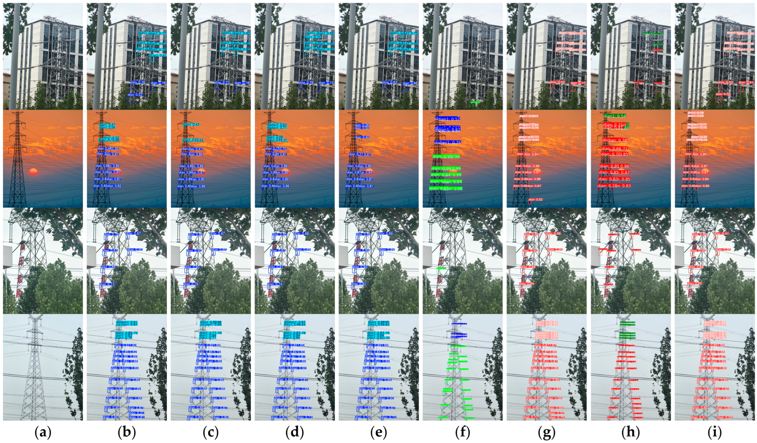
The historical nano-scale comparisons and Figure 10 remain descriptive records rather than capacity-matched evidence. Their full training and timing protocols were not recovered, so they are not merged into the updated numerical comparison.
Figure 10.
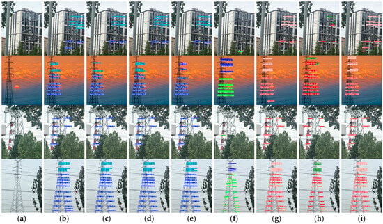
Detection results of different models. (a) Original; (b) YOLO v5n; (c) YOLO v8n; (d) YOLO 11n; (e) YOLO v12n; (f) DETR; (g) RT-DETR-r18; (h) RT-DETR v2-r18; (i) ours.
The originally submitted RT-DETRv2 [29] row reported an AP of 0.601, higher than that of our submitted model at 0.596, but lacked P/R/timing details. The supplied reduced-backbone-learning-rate r18 control gives a recalculated COCOeval AP of 52.32%; it is not an official RT-DETRv2 reproduction. Missing historical DETR and official RT-DETRv2 evaluations remain a limitation, not evidence of superiority.
Table 3 reports a separate local-image timing experiment: batch 1, FP32, actual 640 × 640 input as reported, RTX 3090 GPU0, 100 warmup frames and 489 measured frames (three passes over 163 images). The reported total includes image reading/decoding, preprocessing, transfer, forward inference, postprocessing and result assembly; it excludes network transfer and output writing. Our model takes 66.93 ms per image on average (14.94 FPS), versus 58.76 ms (17.02 FPS) for the baseline. Forward times are 19.16 and 10.85 ms. Reading and decoding together account for about 40 ms; the report does not separate storage access from decoding. The total also contains overhead not individually listed in the stage timings. RT-DETR postprocessing is NMS-free; YOLO postprocessing must be described separately. These measurements describe this desktop file-input pipeline, not an airborne acquisition-to-control system. The earlier 47.16 figure was computed as 1000 divided by the sum of preprocessing, inference and postprocessing medians (1.94, 18.89 and 0.38 ms); it was neither pure-forward throughput nor full-pipeline throughput. A universal 30 FPS real-time claim is not made.
Figure 10 contains four image rows comparing the original image and listed models. Predictions are local boxes for the upper-region class dian1 and lower-region class dian. These examples illustrate urban-background, sunset, vegetation-occlusion and tower-structure conditions. They supplement quantitative image-space evaluation and do not independently measure whole-tower detection or three-dimensional accuracy. Ground-truth examples and the exact upper/lower rule must accompany the final figure.
The first row shows tower structures against buildings and vegetation. Predictions consist of several local boxes on one tower. They must be interpreted according to Section 2 and cannot independently establish detection of distant whole towers.
The second row shows a sunset image with varying contrast. False positives and false negatives require comparison with ground truth under a common evaluation protocol. A single illustration cannot determine average robustness to low light.
The third row includes vegetation and partial occlusion. The fourth shows multiple local positions along a tower. Localization comparisons require ground-truth boxes and matched criteria; confidence labels and visual placement alone do not demonstrate higher IoU.
These examples illustrate model behavior. Interpretation is limited by image selection, annotation definition, and visualization settings, and requires held-out quantitative evaluation and failure-case analysis.
4.4. Ablation Study
Table 4 retains the submitted eight-configuration ablation for transparency, with corrected total parameter counts before inference fusion. Mod 1 denotes the backbone intervention, Mod 2 AIFI_DAttention, and Mod 3 jointly SBA_fused and P2. Historical FPS lacks a recovered timing protocol and is not comparable with Table 3. Table 5 compares four P2/SBA configurations across three seeds. Table 6 reports the separate three-seed backbone-block comparison.
Table 4.
Historical grouped ablation with corrected parameter counts. FPS is historical and not protocol-matched to the new timing experiment.
Table 5.
P2 and SBA_fused ablation on the fixed private validation split. Bbox AP and small-object AP (APs) are percentages. Summary values are the mean ± sample standard deviation over seeds 0, 1, and 2.
Table 6.
New four-variant backbone-block comparison on the private validation split, three seeds. Values are mean ± sample standard deviation in percent; all variants omit P2/SBA and share the audited decoder configuration.
Mod 1 changes submitted AP50/AP from 0.906/0.567 to 0.912/0.570. Corrected parameters are 20.0843 M for the baseline and 13.7515 M for Mod 1; these grouped changes do not isolate SHSA or CGLU.
Mod 2 gives a submitted AP 0.575 and 20.0878 M parameters (20.09 M to two decimal places). The small parameter change is not evidence of equal computation cost.
Mod 3 gives a submitted AP of 0.575 and 20.8466 M parameters. Table 5 separates the P2 and SBA configuration choices under a common training and evaluation protocol.
The final configuration has the highest reported AP50 and recall among these ablations. Interactions are not uniformly beneficial: Mod 1 plus Mod 2 gives strict mAP 0.563, below baseline 0.567. The full-model result does not imply every combination improves every metric. Repeated runs and constituent controls are needed to assess stability.
Table 5 compares B0 (neither P2 nor SBA), B1 (P2 only), B2 (SBA only), and B3 (P2 and SBA). All four configurations share the C2f_SHSA_CGLU backbone, deformable encoder attention, and a decoder with hidden dimension 128, 300 queries, and three layers. P2 adds a fourth input feature level to the decoder. The joint B3 configuration has six SBA fusion stages, compared with four in B2, because it also routes the P2 level through the fusion network. The comparison therefore measures the specified configurations.
B3 has the highest AP for each seed. Its mean AP is 58.33%, 2.67 percentage points above B0, with 5.30 M additional parameters. Its mean small-object AP is 49.37%, compared with 43.78% for B0. Relative to B0, P2 alone and SBA alone increase mean AP by 1.49 and 0.58 percentage points, respectively, and each lowers AP in one of the three seeds. This supports the joint configuration on the reported validation split. The individual effects vary by seed, and the differing fusion depth limits interpretation of the combination as an interaction between independent factors.
The backbone controls in Table 6 use a separate three-level decoder with hidden dimension 128 and omit P2 and SBA. Their reported scores come from the earlier evaluation of those backbone configurations.
All four new block variants were trained from random initialization for seeds 0, 1 and 2 under the same private-task protocol. Table 6 reports an AP of 55.59 ± 0.67% for plain C2f, 55.98 ± 0.82% for SHSA-only, 55.38 ± 0.63% for DWConv+CGLU, and 55.67 ± 0.68% for SHSA+CGLU. The composite is +0.0818 points relative to plain C2f with mixed seed directions, −0.3088 points relative to SHSA-only, and +0.2823 points relative to DWConv+CGLU. The last difference is positive in all three seeds but is not a significance test. The composite reduces parameters by about 14.18% relative to plain C2f, while SHSA-only has slightly fewer parameters and higher mean AP. Thus these controls do not demonstrate a consistent CGLU accuracy benefit or universal synergy, and do not establish this assembly as optimal. The no-SHSA control also removes its associated normalization/attention path; the four replacements are not a perfectly matched mathematical two-factor experiment.
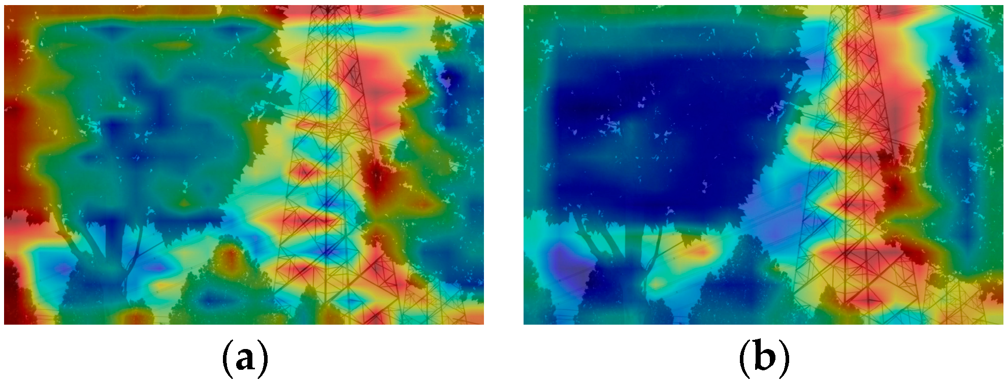
Feature-response heatmaps are qualitative. Warm and cool colors denote high and low displayed responses under the selected aggregation and normalization. They do not measure causal background suppression, detection correctness, or computation. Extraction layer, aggregation, scaling, interpolation, and normalization must be reported.
For qualitative inspection, Figure 11 compares P5 feature responses from the baseline and a backbone-modified model in a selected vegetation-occlusion scene. It is not an independent test of SHSA or CGLU and does not override the quantitative block comparison.
Figure 11.
Visual comparison of backbone feature maps. (a) Backbone feature map of the baseline model; (b) Backbone feature map after incorporating the C2f-SHSA-CGLU module.
Figure 11a shows responses in tower and surrounding vegetation regions. This selected example should not be generalized without quantitative evaluation.
Figure 11b shows a different response distribution after the backbone intervention. Common extraction and normalization are necessary for interpretation. The visualization does not isolate gating or establish a causal explanation of the accuracy change.
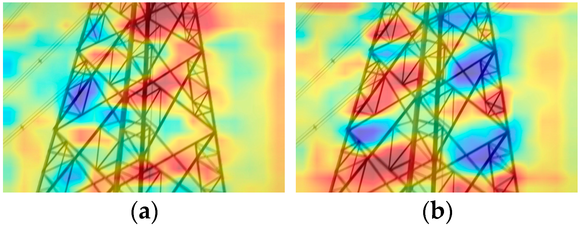
Figure 12 compares selected encoder-stage feature-response maps displayed with Min–Max normalization. Differences in visible response patterns are illustrative and do not establish causal background suppression, universal alignment with lattice edges or computational savings.
Figure 12.
Visual comparison of attention mechanism feature maps. (a) Attention map of the AIFI module in the baseline model; (b) Attention map after incorporating the aifi_DAttention module.
Figure 12a includes responses in tower-framework regions. Response intensity depends on extraction and normalization.
Figure 12b shows a different pattern near parts of the structure. This illustrative comparison requires a common protocol. It does not establish that all offsets align with edges or that computational redundancy is reduced.
4.5. Size-Specific and Error Analysis
Table 7 reports recalculated COCOeval metrics on the 163-image private validation split (2504 instances), using the existing predictions, conf = 0.001, reported iou = 0.7, max_det = 300 and COCOeval maxDets values 1, 10 and 300. GT annotation identifiers were reassigned from zero-based to unique positive integers to avoid collision with COCOeval’s unmatched marker; boxes, areas, classes, images and predictions were unchanged. The small/medium/large counts are 638/1310/556 in original-image coordinates. Our seed 0 gives an AP of 59.14%, AP50 92.13%, AP_small 52.06%, AP_medium 59.77% and AP_large 72.03%, versus 56.68%, 90.79%, 44.88%, 58.55% and 72.37% for RT-DETR-r18. The AP changes are +2.45 points overall, +7.18 small, +1.22 medium and −0.34 large. These validation results are distinct from public COCO-dataset evaluation and from the earlier Ultralytics metrics. A small image area does not verify physical imaging distance.
Table 7.
Earlier COCOeval metrics on the private validation split. Values are percentages. The P2/SBA rows are historical single-run results, separate from the FP32 three-seed comparison in Table 5. The lower-backbone-LR row is an r18 training-setting control.
Table 8 gives the existing confusion matrix at confidence 0.25 and IoU 0.45, with predictions as rows and ground truth as columns. It contains 1537 correct dian matches, 823 correct dian1 matches, 38 cross-class matches, 106 unmatched ground-truth instances and 635 unmatched predictions. Cross-class errors also contribute to class-specific false positives and false negatives. These fixed-threshold counts are not interchangeable with the P/R operating point in Table 2. The selected visual examples in Figure 10, Figure 11 and Figure 12 are qualitative; neither the prevalence of specific failure causes nor imaging distances has been quantified.
Table 8.
Confusion matrix counts at confidence 0.25 and IoU 0.45; predicted classes are rows.
4.6. Statistical Stability Across Random Seeds
Table 9 retains the earlier Ultralytics three-seed results. The mean differences between our model and the baseline are +1.70 percentage points for AP50 and +1.72 for AP. Table 5 and Table 6 report separate COCOeval ablations on the private validation split, and Table 10 and Table 11 report public-task results over three seeds. The sample standard deviations describe variability across training seeds on fixed splits. They provide no estimate of variability across independent scenes.
Table 9.
Earlier Ultralytics evaluation over three seeds, mean ± sample standard deviation. These values are not pooled with Table 7.
Table 10.
STN PLAD supplementary test results over three seeds, mean ± sample standard deviation in percent. Test set: 25 images and 582 instances. This five-class task differs from the private structural-region labels.
Table 11.
STN PLAD per-class test AP over three seeds, mean ± sample standard deviation in percent. Class counts are shown in the header.
4.7. Supplementary Public Asset Detection
Table 10 and Table 11 report the STN PLAD test results of the selected FP32 EMA checkpoints. We used bbox COCOeval over IoU thresholds 0.50 to 0.95 in steps of 0.05, with maxDets = 300 in original-image coordinates. For production inference, each image was resized directly to 640 × 640 without padding, converted to RGB, and scaled to [0, 1]. Both models used the same batch-one FP32 fused inference path with a confidence threshold of 0.001 and no non-maximum suppression. Test AP for RT-DETR-r18 was 42.7951%, 44.4797%, and 45.2685% for seeds 0, 1, and 2, respectively. Our model achieved 39.0045%, 41.1216%, and 32.4691%. Our model had a lower overall AP in all three paired seeds and a lower mean AP for each of the five classes. Two individual class–seed comparisons favored our model (plate for seed 0 and insulator for seed 1). Our model also showed larger seed variation in overall AP. Small-object AP was below 1% on average for both models.
On STN PLAD, the proposed architecture underperforms RT-DETR-r18 under the reported protocol. With fusion enabled, the mean AP deficit is 6.65 percentage points. With fusion disabled, the deficit is 6.68 points (37.50% for our model and 44.18% for RT-DETR-r18). The result limits the architectural claim to the improvements observed under the private validation protocol. The public experiment uses five asset categories, whereas the private task localizes two structural regions within towers. It provides evidence on a separate detection task, and the transfer of dian and dian1 to independent scenes remains unverified. The distinct initialization histories also limit attribution of the public AP gap to any individual architectural component.
We audited the six saved public FP32 EMA checkpoints without retraining or modifying their states. The production-path replay reproduced all six test AP values exactly. Across 552 image-level forward passes covering 21 validation and 25 test images, six checkpoints, and both fusion states, the recorded primary outputs, auxiliary outputs, and exported predictions were finite. Mean fused-minus-unfused test AP was +0.0013 percentage points for RT-DETR-r18 and +0.0313 for our model. For our seed 2, the 0.1056-point discrepancy concerned the internal validation mAP50–95. It comprises +0.0982 points from fused versus unfused validation and +0.0074 from unfused validation versus the training record. The same seed showed a +0.0020-point fusion effect on test COCOeval AP.
The synthetic standard–normal input produced 8100 nonfinite output values per inference state in our seed 2 and in a separate smoke-test checkpoint of our model. The matched uniform [0, 1] input yielded finite outputs. The first detected nonfinite module output was the fc2 projection in an SBA_fused block, which already received nonfinite input. The activation trace and the float64 control support FP32 overflow in the SE-weighted feature multiplication. Clamping the batch-normalization variances alone did not remove the anomaly. These diagnostics bound the numerical-stability claim. The audited real-image runs show no evidence that this synthetic anomaly affected the reported STN PLAD test AP.
4.8. Limitations and Deployment Boundaries
The 163-image private split serves both checkpoint selection and performance reporting, and the private task has no independent test partition. The available records cannot confirm complete separation of source videos or physical towers between training and validation. Inter-annotator agreement and reliable weather and location subgroup labels were unavailable. Repeated training seeds describe variability on the same split. The public comparison covers a different label set, has different initialization histories for the two models, and uses a previously inspected test partition. Its negative result limits the scope of the observed private validation gains. The numerical audit covers the six public FP32 EMA checkpoints and the specified real images. Per-image numerical stability of the historical private FP16 checkpoints remains unverified. The reduced-backbone-learning-rate r18 control is distinct from an official RT-DETRv2 evaluation [29]. Desktop timing leaves onboard operation, closed-loop rangefinder alignment, and downstream three-dimensional tilt accuracy unverified.
5. Conclusions
This work adapts RT-DETR for two-class localization of transmission tower structural regions. On the private validation split, our seed 0 achieves a 59.14% AP and a 52.06% small-object AP, compared with 56.68% and 44.88% for RT-DETR-r18. The four-variant backbone comparison shows no consistent CGLU accuracy benefit.
Per-image numerical stability remains unverified for the historical private FP16 checkpoints underlying the primary validation results, including the result of our seed 0 in Table 7.
The joint P2/SBA configuration leads in all three private validation seeds, gaining 2.67 AP percentage points over omitting both at a cost of 5.30 M parameters. On STN PLAD, our model trails RT-DETR-r18 by 6.65 points with fusion and 6.68 points without fusion. The private split serves both checkpoint selection and performance reporting. Performance on independent scenes, onboard operation, and downstream measurement accuracy remain unverified.
Author Contributions
X.H. designed the methodology. H.C. developed the software and conducted the experiments. R.L. prepared the original draft. T.Z. provided the data. Y.C. carried out the fieldwork. X.K. verified the results. M.Y. reviewed the manuscript. All authors have read and agreed to the published version of the manuscript.
Funding
This research received no external funding.
Data Availability Statement
The public STN PLAD dataset is available at https://github.com/andreluizbvs/PLAD (accessed on 11 November 2026). The private transmission tower images and annotations are used in an industry collaboration project and are unavailable for public release.
Conflicts of Interest
Authors Ting Zeng, Yueqing Chen, Xiangmei Kong and Mingpeng Yuan were employed by Shantou Power Supply Bureau of Guangdong Power Grid Co., Ltd. The remaining authors declare that the research was conducted in the absence of any commercial or financial relationships that could be construed as a potential conflict of interest.
References
- Shen, Y.; Zhou, Q.; Wen, Y.; Shuai, Z.; Shen, Z.J. Integrated Satellite-Terrestrial Network Framework for Next Generation Smart Grid. IEEE Trans. Smart Grid 2024, 15, 5249–5252. [Google Scholar] [CrossRef] [Scilit]
- Lu, Y.; Li, D.; Li, D.; Li, X.; Gao, Q.; Yu, X. A Lightweight Insulator Defect Detection Model Based on Drone Images. Drones 2024, 8, 431. [Google Scholar] [CrossRef] [Scilit]
- Wang, B.; Li, C.; Zou, W.; Zheng, Q. Foreign Object Detection Network for Transmission Lines from Unmanned Aerial Vehicle Images. Drones 2024, 8, 361. [Google Scholar] [CrossRef] [Scilit]
- Mendu, B.; Mbuli, N. State-of-the-Art Review on the Application of Unmanned Aerial Vehicles (UAVs) in Power Line Inspections: Current Innovations, Trends, and Future Prospects. Drones 2025, 9, 265. [Google Scholar] [CrossRef] [Scilit]
- Şener, A.; Tümen, V.; Ergen, B.; Akin, E. CalFireSegNet: A Lightweight Hybrid Attention–Transformer Network for Post-Wildfire Building Footprint Change Analysis Using High-Resolution Satellite Imagery. Sci. Rep. 2026, 16, 25725. [Google Scholar] [CrossRef] [Scilit] [PubMed]
- Cheng, K.; Cui, Y.; Liu, Y.; Yin, P.; Jiang, Y.; Liu, N.; Yin, Z.; Wu, J.; Zhao, T.; Tan, J. SBG-DDN: Semantic Boundary-Guided Dynamic Detection Network for Small Transmission Tower Detection in Remote Sensing Images. Remote Sens. 2026, 18, 1452. [Google Scholar] [CrossRef] [Scilit]
- Bellou, E.; Pisica, I.; Banitsas, K. Aerial Inspection of High-Voltage Power Lines Using YOLOv8 Real-Time Object Detector. Energies 2024, 17, 2535. [Google Scholar] [CrossRef] [Scilit]
- Wang, W.; Wang, Q. No Tower Information Needed: An Autonomous Inspection Route Generation Method Based on Target Detection. Artif. Life Robot. 2026, 31, 149–158. [Google Scholar] [CrossRef] [Scilit]
- Zhang, L.; Zhang, Y.; Tang, S.; He, W.; Zhang, T.; Hu, Y. A Precision Detection Method for Key Components of Power Transmission Towers Oriented to UAV Autonomous Localization. J. Beijing Inst. Technol. 2025, 34, 590–601. [Google Scholar] [CrossRef]
- Girshick, R.; Donahue, J.; Darrell, T.; Malik, J. Rich Feature Hierarchies for Accurate Object Detection and Semantic Segmentation. In Proceedings of the IEEE Conference on Computer Vision and Pattern Recognition (CVPR), Columbus, OH, USA, 23–28 June 2014; pp. 580–587. Available online: https://openaccess.thecvf.com/content_cvpr_2014/html/Girshick_Rich_Feature_Hierarchies_2014_CVPR_paper.html (accessed on 11 November 2026).
- Girshick, R. Fast R-CNN. In Proceedings of the IEEE International Conference on Computer Vision (ICCV), Santiago, Chile, 13–16 December 2015; pp. 1440–1448. Available online: https://openaccess.thecvf.com/content_iccv_2015/html/Girshick_Fast_R-CNN_ICCV_2015_paper.html (accessed on 11 November 2026).
- Ren, S.; He, K.; Girshick, R.; Sun, J. Faster R-CNN: Towards Real-Time Object Detection with Region Proposal Networks. IEEE Trans. Pattern Anal. Mach. Intell. 2017, 39, 1137–1149. [Google Scholar] [CrossRef] [Scilit] [PubMed]
- He, K.; Gkioxari, G.; Dollár, P.; Girshick, R. Mask R-CNN. In Proceedings of the IEEE International Conference on Computer Vision (ICCV), Venice, Italy, 22–29 October 2017; pp. 2961–2969. Available online: https://openaccess.thecvf.com/content_iccv_2017/html/He_Mask_R-CNN_ICCV_2017_paper.html (accessed on 11 November 2026).
- Redmon, J.; Divvala, S.; Girshick, R.; Farhadi, A. You Only Look Once: Unified, Real-Time Object Detection. In Proceedings of the IEEE Conference on Computer Vision and Pattern Recognition (CVPR), Las Vegas, NV, USA, 27–30 June 2016; pp. 779–788. Available online: https://openaccess.thecvf.com/content_cvpr_2016/html/Redmon_You_Only_Look_CVPR_2016_paper.html (accessed on 11 November 2026).
- Wang, A.; Chen, H.; Liu, L.; Chen, K.; Lin, Z.; Han, J.; Ding, G. YOLOv10: Real-Time End-to-End Object Detection. In Advances in Neural Information Processing Systems; Curran Associates, Inc.: Red Hook, NY, USA, 2024; Volume 37, pp. 107984–108011. [Google Scholar] [CrossRef] [Scilit]
- Tian, Y.; Ye, Q.; Doermann, D. YOLOv12: Attention-Centric Real-Time Object Detectors. In Advances in Neural Information Processing Systems; Curran Associates, Inc.: Red Hook, NY, USA, 2025; Volume 38, Main Conference; pp. 78433–78457. [Google Scholar] [CrossRef] [Scilit]
- Liu, W.; Anguelov, D.; Erhan, D.; Szegedy, C.; Reed, S.; Fu, C.-Y.; Berg, A.C. SSD: Single Shot MultiBox Detector. In Computer Vision—ECCV 2016; Lecture Notes in Computer Science; Springer: Cham, Switzerland, 2016; Volume 9905, pp. 21–37. [Google Scholar] [CrossRef] [Scilit]
- Lin, T.-Y.; Goyal, P.; Girshick, R.; He, K.; Dollár, P. Focal Loss for Dense Object Detection. In Proceedings of the IEEE International Conference on Computer Vision (ICCV), Venice, Italy, 22–29 October 2017; pp. 2980–2988. Available online: https://openaccess.thecvf.com/content_iccv_2017/html/Lin_Focal_Loss_for_ICCV_2017_paper.html (accessed on 11 November 2026).
- Carion, N.; Massa, F.; Synnaeve, G.; Usunier, N.; Kirillov, A.; Zagoruyko, S. End-to-End Object Detection with Transformers. In Computer Vision—ECCV 2020; Lecture Notes in Computer Science; Springer: Cham, Switzerland, 2020; Volume 12346, pp. 213–229. [Google Scholar] [CrossRef] [Scilit]
- Zhu, X.; Su, W.; Lu, L.; Li, B.; Wang, X.; Dai, J. Deformable DETR: Deformable Transformers for End-to-End Object Detection. In Proceedings of the International Conference on Learning Representations (ICLR), Virtual Event, 3–7 May 2021; Available online: https://openreview.net/forum?id=gZ9hCDWe6ke (accessed on 11 November 2026).
- Zhao, Y.; Lv, W.; Xu, S.; Wei, J.; Wang, G.; Dang, Q.; Liu, Y.; Chen, J. DETRs Beat YOLOs on Real-time Object Detection. In Proceedings of the IEEE/CVF Conference on Computer Vision and Pattern Recognition (CVPR), Seattle, WA, USA, 17–21 June 2024; pp. 16965–16974. Available online: https://openaccess.thecvf.com/content/CVPR2024/html/Zhao_DETRs_Beat_YOLOs_on_Real-time_Object_Detection_CVPR_2024_paper.html (accessed on 11 November 2026).
- Vieira-e-Silva, A.L.B.; Felix, H.; Chaves, T.M.; Simões, F.P.M.; Teichrieb, V.; dos Santos, M.M.; Santiago, H.C.; Sgotti, V.A.C.; Lott Neto, H.B.D.T. STN PLAD: A Dataset for Multi-Size Power Line Assets Detection in High-Resolution UAV Images. In Proceedings of the 34th SIBGRAPI Conference on Graphics, Patterns and Images, Virtual Event, 18–22 October 2021; pp. 215–222. [Google Scholar] [CrossRef] [Scilit]
- Yun, S.; Ro, Y. SHViT: Single-Head Vision Transformer with Memory Efficient Macro Design. In Proceedings of the IEEE/CVF Conference on Computer Vision and Pattern Recognition (CVPR), Seattle, WA, USA, 17–21 June 2024; pp. 5756–5767. Available online: https://openaccess.thecvf.com/content/CVPR2024/html/Yun_SHViT_Single-Head_Vision_Transformer_with_Memory_Efficient_Macro_Design_CVPR_2024_paper.html (accessed on 11 November 2026).
- Shi, D. TransNeXt: Robust Foveal Visual Perception for Vision Transformers. In Proceedings of the IEEE/CVF Conference on Computer Vision and Pattern Recognition (CVPR), Seattle, WA, USA, 17–21 June 2024; pp. 17773–17783. Available online: https://openaccess.thecvf.com/content/CVPR2024/html/Shi_TransNeXt_Robust_Foveal_Visual_Perception_for_Vision_Transformers_CVPR_2024_paper.html (accessed on 11 November 2026).
- Xia, Z.; Pan, X.; Song, S.; Li, L.E.; Huang, G. Vision Transformer with Deformable Attention. In Proceedings of the IEEE/CVF Conference on Computer Vision and Pattern Recognition (CVPR), New Orleans, LA, USA, 21–24 June 2022; pp. 4794–4803. Available online: https://openaccess.thecvf.com/content/CVPR2022/html/Xia_Vision_Transformer_With_Deformable_Attention_CVPR_2022_paper.html (accessed on 11 November 2026).
- Tang, F.; Xu, Z.; Huang, Q.; Wang, J.; Hou, X.; Su, J.; Liu, J. DuAT: Dual-Aggregation Transformer Network for Medical Image Segmentation. In Pattern Recognition and Computer Vision (PRCV 2023); Lecture Notes in Computer Science; Springer: Singapore, 2024; Volume 14429, pp. 343–356. [Google Scholar] [CrossRef] [Scilit]
- Wu, T.; Tang, S.; Zhang, R.; Cao, J.; Zhang, Y. CGNet: A Light-Weight Context Guided Network for Semantic Segmentation. IEEE Trans. Image Process. 2021, 30, 1169–1179. [Google Scholar] [CrossRef] [Scilit] [PubMed]
- Hu, J.; Shen, L.; Sun, G. Squeeze-and-Excitation Networks. In Proceedings of the IEEE Conference on Computer Vision and Pattern Recognition (CVPR), Salt Lake City, UT, USA, 19–21 June 2018; pp. 7132–7141. Available online: https://openaccess.thecvf.com/content_cvpr_2018/html/Hu_Squeeze-and-Excitation_Networks_CVPR_2018_paper.html (accessed on 11 November 2026).
- Lv, W.; Zhao, Y.; Chang, Q.; Huang, K.; Wang, G.; Liu, Y. RT-DETRv2: Improved Baseline with Bag-of-Freebies for Real-Time Detection Transformer. arXiv 2024, arXiv:2407.17140. [Google Scholar] [CrossRef] [Scilit]

Disclaimer/Publisher’s Note: The statements, opinions and data contained in all publications are solely those of the individual author(s) and contributor(s) and not of MDPI and/or the editor(s). MDPI and/or the editor(s) disclaim responsibility for any injury to people or property resulting from any ideas, methods, instructions or products referred to in the content. |
© 2026 by the authors. Licensee MDPI, Basel, Switzerland. This article is an open access article distributed under the terms and conditions of the Creative Commons Attribution (CC BY) license.