Reconstruction of Boolean Networks Using Input–Output Data Sets

Abstract

Boolean networks (BNs) are widely used to model gene regulatory networks. In practice, however, their internal states can rarely be measured directly, and the available output measurements are corrupted by noise. In this paper, we propose a data-driven framework for reconstructing the output trajectories and identifying the initial states of a BN using only input–output datasets under probabilistic bit-flip observation noise. The proposed framework consists of two steps. First, noisy output sequences obtained from repeated experiments are vectorized and partitioned into clusters by K-means clustering, and principal component analysis (PCA) is used to visualize their separability. Second, the noise within each cluster is removed by averaging and thresholding, which is justified by the law of large numbers, and the reconstructed trajectory is matched with a reference library of noise-free trajectories using the Hamming distance to identify the corresponding initial state. The effectiveness of the proposed method is demonstrated through numerical examples, including a BN model of the mammalian cell cycle. When there are three candidate initial states, all trajectories and initial states are correctly reconstructed, whereas when the number of candidates increases to seven, only two of them are identified, revealing a limitation of the K-means-based approach.

1. Introduction

Systems biology studies biological processes from a system-level perspective, emphasizing interactions among components rather than isolated molecular events [1]. This viewpoint is particularly important for understanding complex phenomena such as robustness, adaptation, and cellular decision-making [2,3,4]. Since many such dynamics are difficult to observe directly, mathematical and computational models play an essential role in integrating experimental data and analyzing system behavior.

Gene Regulatory Networks (GRNs) provide a natural framework for describing how genes and regulatory factors interact through activation and inhibition [5,6]. Depending on the available data and modeling objectives, GRNs can be represented by continuous, hybrid, or discrete models. In many biological applications, however, detailed kinetic parameters are unavailable, making qualitative logic-based models especially useful [7,8].

Among such discrete models, Boolean Networks (BNs) are widely used for GRN analysis. In a BN, each gene is represented by a binary variable, and its evolution is determined by Boolean functions of its regulators [9]. Although simple, BNs can capture important dynamical features such as multiple stable states, oscillations, and attractors, which are often interpreted as cellular phenotypes [10,11]. Accordingly, many studies have focused on attractor analysis, state-space reduction, and the influence of network structure on long-term behavior [12,13].

In addition to analyzing intrinsic dynamics, increasing attention has been paid to control and observation problems in BNs. A substantial body of research has investigated the observability of Boolean networks (BNs) and Boolean control networks (BCNs). For example, Liu et al. [14] proposed a graph-based approach to minimal observability, addressing both observability verification and the selection of additional measurements required to make a system observable. Zhang [15] provided a comprehensive survey of observability theories and verification methods for BCNs, including graph-based and algebraic approaches. These studies establish important theoretical foundations for determining whether an initial state can be uniquely inferred from the corresponding output sequence. However, their primary focus is on observability analysis and measurement design, rather than on reconstructing noise-free output trajectories from repeated input–output measurements corrupted by probabilistic observation noise.

Related research has also addressed reconstruction problems involving noisy Boolean dynamics. Kobayashi and Wu [16] studied the reconstruction of noisy dynamics and the estimation of selection probabilities in probabilistic BNs, given the main dynamics and sample means obtained from noisy experimental data. In contrast, this paper considers a known BN model with probabilistic observation noise and focuses on recovering the noise-free output trajectories and identifying the corresponding initial states from repeated noisy input–output datasets. Since the internal states are not directly observed, the noisy trajectories associated with different initial states must first be distinguished before the underlying output sequences can be reconstructed.

The authors’ previous conference work [17] considered a restricted class of BNs for which grouping the observed trajectories was unnecessary. The present work addresses a more general setting in which noisy output trajectories generated from multiple unknown initial states are mixed in the observed dataset. To address this problem, we propose a framework that combines K-means clustering of vectorized output trajectories, cluster-wise averaging and thresholding for noise reduction, and Hamming-distance matching with a reference library of noise-free trajectories. Principal component analysis (PCA) is used to visualize the clustering results, rather than to perform dimensionality reduction before clustering. The main contributions of this paper are summarized as follows:

• We formulate a reconstruction problem in which the internal states are not directly measurable and the available repeated input–output observations are corrupted by probabilistic bit-flip noise.
• We develop an integrated reconstruction framework that groups noisy output trajectories using K-means, reconstructs representative noise-free trajectories through cluster-wise averaging and thresholding, and identifies the corresponding initial states by matching the reconstructed trajectories with a model-based reference library using the Hamming distance.
• We evaluate the proposed method using numerical experiments, including comparisons with direct nearest-reference matching, sensitivity analyses under different noise levels, numbers of candidate initial states, and observation horizons, as well as measurements of execution time and peak memory usage.

2. Preliminaries and Problem Formulation

A BN is a standard framework for modeling complex regulatory systems, particularly GRNs. It is defined as a discrete-time dynamical system on a directed graph with a set of binary-valued nodes $\mathcal{N}=\{1,2,\dots ,n\}$. The state of the i-th node at time k, denoted by $x_i\left(k\right)\in \{0,1\}$, represents the expression level (e.g., active or inactive) of a specific gene. The global system state is the vector $x\left(k\right):={[x_1\left(k\right),\dots ,x_n\left(k\right)]}^{\top }\in {\{0,1\}}^n$. The temporal evolution of the network is governed by a set of coupled Boolean functions:

$$\mathcal{F}:x_i(k+1)=f^{\left(i\right)}\left(x\left(k\right)\right),i\in \mathcal{N},k=0,1,2,\dots ,$$

(1)

where the update function $f^{\left(i\right)}:{\{0,1\}}^n\to \{0,1\}$ is constructed using basic logical operators such as AND (∧), OR (∨), and NOT (¬), reflecting the regulatory logic of the system. We remark that in this paper, the Boolean values False and True are identified with 0 and 1, and a Boolean function may be regarded as a real-valued function through its (unique) multilinear extension. In particular, consider the evolution of a BN over a finite time interval of length T, that is, $k\in \{0,1,\dots ,T\}$. The state $x\left(0\right)$ is called the initial state of a run over this interval.

In realistic experimental settings, the internal state variables $x\left(k\right)$ are often hidden and cannot be measured directly. Instead, the system is monitored through a set of input and output channels. Let $u\left(k\right)\in {\{0,1\}}^m$ denote the external control input and $y\left(k\right)\in {\{0,1\}}^r$ denote the measurable output. Under this setting, the BN model (1) is extended to the following state-space representation:

$$\left\{\begin{array}{cc}\hfill x(k+1)& = f\left(x\right(k),u(k\left)\right)\hfill \\ \hfill y\left(k\right)& = g\left(x\right(k\left)\right),\hfill \end{array}\right.$$

(2)

where $f:{\{0,1\}}^{n+m}\to {\{0,1\}}^n$ is a given Boolean function, and $g\left(x\left(k\right)\right):=[g^{\left(1\right)}\left(x\left(k\right)\right),\dots ,$$g^{\left(r\right)}{\left(x\left(k\right)\right)]}^{\top }$ is the observation function mapping the internal state to the output space.

In biological assays and signal transmission, measurements are inevitably corrupted by stochastic noise. We conceptually distinguish between the main dynamics, which follow the deterministic BN (2), and the noisy dynamics, which introduce stochastic perturbations; both take Boolean values. The observed output is modeled as a probabilistic mixture. For the j-th output channel at time k, the observed value ${\tilde{y}}_j\left(k\right)$ is a realization of a Bernoulli random variable:

$${\tilde{y}}_j\left(k\right)=\left\{\begin{array}{ccc}{g}^{\left(j\right)}\left(x\left(k\right)\right)\hfill & \hfill & \mathrm{with}\mathrm{probability}{c}_j\left(k\right)\hfill \\ \neg g^{\left(j\right)}\left(x\left(k\right)\right)\hfill & \hfill & \mathrm{with}\mathrm{probability}1-c_j\left(k\right).\hfill \end{array}\right.$$

(3)

The term $\neg g^{\left(j\right)}\left(x\left(k\right)\right)$ represents a “bit-flip” error caused by noise (e.g., $\neg 0=1$). This model assumes that, although the underlying biological process is deterministic, the observation channel introduces an independent stochastic error at each time step. We define $\tilde{y}\left(k\right):={[{\tilde{y}}_1\left(k\right),{\tilde{y}}_2\left(k\right),\dots ,{\tilde{y}}_r\left(k\right)]}^{\top }$. Given the time horizon T, the input sequence is defined as follows:

$$U_T={[u\left(0\right),u\left(1\right),\dots ,u(T-1)]}^{\top }.$$

(4)

When this input sequence is applied to a BN starting from the initial state $x\left(0\right)$, the noisy output $\tilde{y}\left(k\right)$ is observed at each time step. The corresponding output sequence over T steps is defined as

$$Y(x\left(0\right),U_T)={[\tilde{y}\left(1\right),\tilde{y}\left(2\right),\dots ,\tilde{y}\left(T\right)]}^{\top }.$$

(5)

Consider generating the output sequence N times, where the initial state $x\left(0\right)\in {\mathcal{X}}_0$ is randomly chosen in each run and the same input sequence is used in all runs. Let $Y^i$ denote the result of the i-th simulation/experiment. We thus obtain the output dataset $\mathcal{Y}=\{Y^1,\dots ,Y^N\}$.

Under the above setting, the following assumptions are made for the BN (2), (3).

Assumption 1.

The number q of candidate initial states is given.

Assumption 2.

The probability $c_j\left(k\right)$ in (3) satisfies $c_j\left(k\right)\in (0.5,1]$.

Assumption 2 ensures that the true output $y_j\left(k\right)=g^{\left(j\right)}\left(x\left(k\right)\right)$ appears more frequently than its flipped value $\neg g^{\left(j\right)}\left(x\left(k\right)\right)$. Our goal is to remove the noise from the data and to reconstruct the true evolution of the system using the dataset $\mathcal{Y}$. This task is divided into two sequential problems.

The first problem is formulated as follows:

Problem 1.

Suppose that the dataset $\mathcal{Y}$ is given. Partition $\mathcal{Y}$ into q distinct clusters.

In the first problem, we need to show that trajectories starting from different initial states can be separated despite the presence of observation noise in the high-dimensional data. Once the trajectories are successfully separated, the second objective is to reconstruct the true output trajectory from the noisy data, which involves filtering out the stochastic bit flips. Thus, the second problem is formulated as follows:

Problem 2.

Suppose that q distinct clusters are given as a solution to Problem 1. For each cluster, find the true output sequence $y\left(0\right),y\left(1\right),\dots ,y\left(T\right)$ and identify the corresponding initial state corresponding to each cluster.

3. Solution Method

3.1. Solution Method for Problem 1

To address Problem 1, we propose a data-driven framework that combines clustering with PCA-based visualization. We treat the entire temporal evolution of the network not as a sequence of independent states but as a single geometric object (a trajectory) in a high-dimensional Euclidean space.

Suppose that the output data $Y^l(x\left(0\right),U_T)$ are observed in the l-th run of the simulation with the input sequence $U_T$. Here, $Y^l$ is the matrix defined by $Y^l:={[\tilde{y}\left(1\right),\tilde{y}\left(2\right),\dots ,\tilde{y}\left(T\right)]}^{\top }$, where $\tilde{y}\left(k\right)\in {\{0,1\}}^r$ (see (5)). Hence, $Y^l$ is a $T\times r$ matrix. To make the data suitable for computation, we introduce the following vectorization:

$${\mathbf{v}}^l=\mathrm{vec}\left(Y^l\right)\in {\mathbb{R}}^{Tr},l\in \{1,2,\dots ,N\},$$

(6)

by which a point ${\mathbf{v}}^l$ in a $Tr$-dimensional Euclidean space is obtained for the l-th run of the simulation. By applying this vectorization to all elements of $\mathcal{Y}$, we obtain a collection $\mathcal{V}=\{{\mathbf{v}}^1,{\mathbf{v}}^2,\dots ,{\mathbf{v}}^N\}$ of N points in the high-dimensional Euclidean space.

The vectorized trajectories are projected onto a two-dimensional subspace by principal component analysis (PCA) for visualization. Since the candidate initial-state set ${\mathcal{X}}_0$ contains q elements, K-means clustering is applied to the original high-dimensional vectors to obtain q clusters, denoted by $C_1,C_2,\dots ,C_q$. For each cluster $C_i$, $i=1,2,\dots ,q$, its centroid is computed as

$${\mu }_i={\displaystyle \frac{1}{|C_i|}}\sum _{{\mathbf{v}}^l\in C_i}{\mathbf{v}}^l,i=1,2,\dots ,q.$$

(7)

The centroid ${\mu }_i$ represents the average trajectory of the noisy observations assigned to the i-th cluster. Ideally, each centroid corresponds to a trajectory associated with a particular initial state in ${\mathcal{X}}_0$.

The number of clusters, q, is assumed known (Assumption 1) and equals the number of candidate initial states. Using the original high-dimensional vectors avoids discarding features relevant to distinguishing trajectories, since directions of greatest variance need not provide the best separation. In the numerical implementation, K-means uses k-means++ initialization with 10 independent initializations, and the solution with the smallest within-cluster sum of squares is retained. Clustering performance depends on the separation between trajectory groups relative to their within-cluster dispersion; greater observation noise or weaker separation may cause overlap and reduce reconstruction accuracy. A general sufficient condition guaranteeing global success under the considered noise model is beyond the scope of this study.

3.2. Solution Method for Problem 2

Once the dataset $\mathcal{Y}$ has been partitioned into clusters $\{C_1,\dots ,C_q\}$ and their centroids $\{{\mu }_1,\dots ,{\mu }_q\}$ have been obtained, we proceed to Problem 2. The first step is to remove the noise from the output data.

Note that each centroid ${\mu }_i$ is obtained by averaging the vectorized trajectories in cluster $C_i$. Therefore, its matrix form is the average of the output data assigned to the same cluster. For each time step k and output channel j, the averaged observation is given by

$${\mathrm{avg}}_i\left[{\tilde{y}}_j\left(k\right)\right]:={\displaystyle \frac{1}{|{\mathcal{C}}_i|}}\sum _{\mathsf{\ell }:{\mathbf{v}}^{\mathsf{\ell }}\in {\mathcal{C}}_i}{\tilde{y}}_j^{\mathsf{\ell }}\left(k\right),i=1,\dots ,q.$$

(8)

where $\mathrm{avg}\left[{\tilde{y}}_j\left(k\right)\right]\in [0,1]$.

Let $y_{i,j}\left(k\right)\in \{0,1\}$ denote the true output of the j-th output channel at time step k associated with cluster ${\mathcal{C}}_i$. From the noise model (3), the expectation of ${\tilde{y}}_j\left(k\right)$ is given by

$$\mathbb{E}\left[{\tilde{y}}_j^{\mathsf{\ell }}\left(k\right)\right]=c_j\left(k\right)y_{i,j}\left(k\right)+(1-c_j\left(k\right))(1-y_{i,j}\left(k\right)).$$

(9)

Here, the law of large numbers (LLN) is used to justify the averaging process. In general, the LLN states that, when the number of independent repeated observations is sufficiently large, their empirical average approaches the corresponding expected value [18]. Therefore, in this setting, averaging the noisy output over many simulations provides a reliable approximation of its expectation. When the number $|{\mathcal{C}}_i|$ of observations in cluster ${\mathcal{C}}_i$ is sufficiently large, we have

$${\mathrm{avg}}_i\left[{\tilde{y}}_j\left(k\right)\right]\approx c_j\left(k\right)y_{i,j}\left(k\right)+(1-c_j\left(k\right))(1-y_{i,j}\left(k\right)).$$

(10)

Under Assumption 2, the reliability parameter satisfies $c_j\left(k\right)\in (0.5,1]$. Since $g^{\left(j\right)}\left(x\left(k\right)\right)$ is the output of a Boolean function, it takes only the value 0 or 1. Hence, the expected noisy observation is greater than 0.5 when the true output is 1 and smaller than 0.5 when the true output is 0. Therefore, the true output can be recovered by the following thresholding rule:

$${\hat{y}}_{i,j}\left(k\right)=\left\{\begin{array}{cc}1,\hfill & {\mathrm{avg}}_i\left[{\tilde{y}}_j\left(k\right)\right]\ge 0.5,\hfill \\ 0,\hfill & {\mathrm{avg}}_i\left[{\tilde{y}}_j\left(k\right)\right]<0.5.\hfill \end{array}\right.$$

(11)

To quantify the reliability of the denoising procedure with a finite number of observations, we derive an error bound based on Hoeffding’s inequality [19]. Let $M_i=\left|{\mathcal{C}}_i\right|$ denote the number of observations in cluster ${\mathcal{C}}_i$. For this analysis, we assume that all observations in ${\mathcal{C}}_i$ correspond to the same underlying output trajectory and that their bit-flip noise realizations are independent across repeated runs. Under these assumptions, the probability of incorrectly reconstructing an individual output bit satisfies

$$\mathrm{Pr}\left({\hat{y}}_{i,j}\left(k\right)\ne y_{i,j}\left(k\right)\right)\le \exp \left[-2M_i{\left(c_j\left(k\right)-{\displaystyle \frac{1}{2}}\right)}^2\right].$$

(12)

This bound indicates that the probability of an incorrect bit-wise reconstruction decreases exponentially with the number of observations in the cluster, provided that $c_j\left(k\right)>0.5$.

In this way, the bit-flip noise is filtered out through repeated observations, and the underlying noise-free output $g^{\left(j\right)}\left(x\left(k\right)\right)$ is obtained.

After the denoising step, each cluster centroid ${\mu }_i$ yields a reconstructed noise-free output trajectory. This trajectory can be regarded as the original output sequence generated by the BN before the bit-flip observation noise was added. Therefore, the remaining task is to determine which initial state produced this output sequence.

Since the structure and update rules of the BN are known, the network can be simulated from every state under the same input sequence $U_T$. This produces a reference library of noise-free output trajectories, in which each trajectory is associated with one possible initial state. The reconstructed output sequence obtained after denoising is then used to search this library in reverse: rather than observing the initial state directly, we compare the reconstructed trajectory with all simulated reference trajectories and infer which candidate initial state is most likely to have generated it.

For each reconstructed trajectory obtained from a cluster centroid ${\mu }_i$, we compute the Hamming distance between this trajectory and every trajectory in the reference library. The Hamming distance is the number of entries that differ between two binary output sequences. If the minimum Hamming distance is zero, the reconstructed trajectory is identical to a true reference trajectory. In this case, the trajectory is successfully identified, and the associated candidate initial state can be determined accordingly. If the minimum Hamming distance is nonzero, no identical trajectory exists in the reference library, which indicates that the reconstructed trajectory is incorrect.

In simulations where initial states are generated randomly, the generated datasets may contain only p distinct initial states, where p is smaller than the preset number q of candidates. In such cases, several cluster centroids ${\mu }_i$ may be matched to the same reference trajectory and therefore to the same initial state. Through the reverse comparison step, these duplicate matches can be detected, and the q apparent clusters can be reduced to the actual number p of distinct reconstructed initial states.

Furthermore, if two distinct initial states generate identical output trajectories under the same input sequence over the observation horizon, they cannot be distinguished based on the available output data alone. In this case, the proposed method may recover the common output trajectory, but it cannot uniquely identify the corresponding initial state. Therefore, unique initial-state identification requires the candidate initial states to produce distinguishable output trajectories under the available observation conditions. Additional observed variables, a longer observation horizon, or different input sequences may help resolve such ambiguities.

The complete reconstruction procedure is summarized in Algorithm 1.

Algorithm 1 Reconstruction from Noisy Input–Output Datasets

Require: BN model $(f,g)$, output datasets $\mathcal{Y}=\{Y^1,\dots ,Y^N\}$, input sequence $U_T$, candidate initial-state set ${\mathcal{X}}_0=\{{\mathbf{x}}_0^1,\dots ,{\mathbf{x}}_0^q\}$, time horizon T Ensure: Reconstructed noise-free output trajectories and their matched initial states.   1: Vectorize the output matrices in $\mathcal{Y}$.   2: Apply K-means clustering to obtain q clusters and their centroids ${\mu }_i$, and visualize the result by PCA.   3: Denoise each centroid ${\mu }_i$ to obtain a reconstructed output trajectory.   4: Construct the reference library of the BN under the input sequence $U_T$.   5: for each reconstructed trajectory do   6:       Compute the number of mismatched entries between it and each reference trajectory.   7:       Match it to the reference trajectory with the minimum number of mismatches.   8:       if the minimum number of mismatches is 0 then   9:             The reconstructed trajectory is correctly matched. 10:       else 11:             Use the minimum number of mismatches as the reconstruction error. 12:       end if 13: end for 14: return The correctly reconstructed trajectories and the corresponding initial states.

4. Numerical Example

In this section, a BN model of the mammalian cell cycle is used to demonstrate the proposed method. Different parameter settings are tested to examine which factors significantly influence its effectiveness.

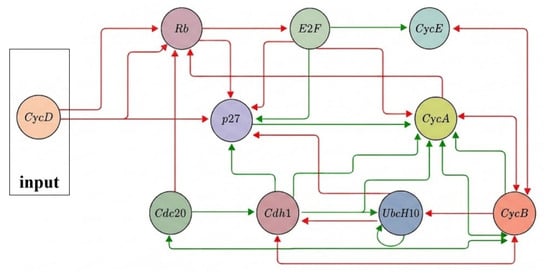
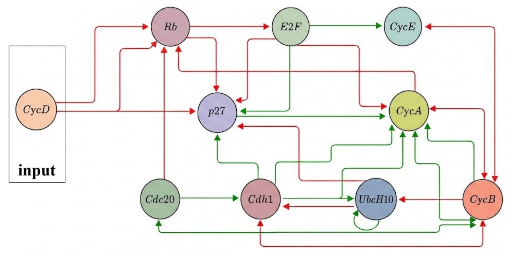
In [20], a BN model that governs the mammalian cell cycle has been established. Its topology is shown in Figure 1. In this BN model, the Boolean states $x_1\left(k\right),\dots ,x_9\left(k\right)$ at time k represent nine proteins, Rb, E2F, CycE, CycA, p27, Cdc20, Cdh1, UbcH10, and CycB, respectively. CycD acts as the input $u\left(k\right)$. The BN dynamics are given by

$${\mathcal{F}}_{mc}:\left\{\begin{array}{cc}\hfill x_1(k+1)& =(\neg u\left(k\right)\wedge \neg x_3\left(k\right)\wedge \neg x_4\left(k\right)\wedge \neg x_9\left(k\right))\vee (x_5\left(k\right)\wedge \neg u\left(k\right)\wedge \neg x_9\left(k\right)),\hfill \\ \hfill x_2(k+1)& =(\neg x_1\left(k\right)\wedge \neg x_4\left(k\right)\wedge \neg x_9\left(k\right))\vee (x_5\left(k\right)\wedge \neg x_1\left(k\right)\wedge \neg x_9\left(k\right)),\hfill \\ \hfill x_3(k+1)& =x_2\left(k\right)\wedge \neg x_1\left(k\right),\hfill \\ \hfill x_4(k+1)& =(x_2\left(k\right)\wedge \neg x_1\left(k\right)\wedge \neg x_6\left(k\right)\wedge x_7\left(k\right)\wedge x_8\left(k\right))\hfill \\ \hfill & \vee (x_4\left(k\right)\wedge \neg x_1\left(k\right)\wedge \neg x_6\left(k\right)\wedge x_7\left(k\right)\wedge x_8\left(k\right)),\hfill \\ \hfill x_5(k+1)& =(\neg u\left(k\right)\wedge \neg x_3\left(k\right)\wedge \neg x_4\left(k\right)\wedge \neg x_9\left(k\right))\vee (x_5\left(k\right)\wedge x_3\left(k\right)\hfill \\ \hfill & \wedge x_4\left(k\right)\wedge \neg u\left(k\right)\wedge \neg x_9\left(k\right)),\hfill \\ \hfill x_6(k+1)& =x_9\left(k\right),\hfill \\ \hfill x_7(k+1)& =(\neg x_4\left(k\right)\wedge \neg x_9\left(k\right))\vee x_6\left(k\right)\vee (x_5\left(k\right)\wedge \neg x_9\left(k\right)),\hfill \\ \hfill x_8(k+1)& =\neg x_7\left(k\right)\vee (x_7\left(k\right)\wedge x_8\left(k\right)\wedge (x_6\left(k\right)\vee x_4\left(k\right)\vee x_9\left(k\right))),\hfill \\ \hfill x_9(k+1)& =\neg x_6\left(k\right)\wedge \neg x_7\left(k\right).\hfill \end{array}\right.$$

(13)

The simulation of ${\mathcal{F}}_{mc}$ is performed over the time horizon T. The input sequence is given as $U_T={[1,1,1,1,1,1,1,1,1,1]}^{\top }$. The number of candidates in ${\mathcal{X}}_0$ is denoted by q, and the number of simulations is N. The detailed hardware and software configurations are specified as follows:

Figure 1. Topology of the mammalian cell cycle.

• Hardware Environment:

  −

  CPU: AMD Ryzen 9 8845H (8 Cores 16 Threads).

  −

  GPU: AMD Radeon 780M.

  −

  Memory: 32 GB DDR5 RAM @ 7500 MT/s.

• Software Environment:

  −

  Operating System: Windows-11-10.0.26200-SP0.

  −

  Programming Language: Python 3.12.2.

4.1. Method Evaluation

The outputs are selected as follows:

$$\left\{\begin{array}{cc}\hfill y_1\left(k\right)=g^{\left(1\right)}\left(x_1\left(k\right)\right)& =x_1\left(k\right),\hfill \\ \hfill y_2\left(k\right)=g^{\left(2\right)}\left(x_2\left(k\right)\right)& =x_2\left(k\right),\hfill \\ \hfill y_3\left(k\right)=g^{\left(3\right)}\left(x_3\left(k\right)\right)& =x_3\left(k\right),\hfill \\ \hfill y_4\left(k\right)=g^{\left(4\right)}\left(x_4\left(k\right)\right)& =x_4\left(k\right),\hfill \\ \hfill y_5\left(k\right)=g^{\left(5\right)}\left(x_5\left(k\right)\right)& =x_5\left(k\right).\hfill \end{array}\right.$$

(14)

Observation noise is introduced as follows:

$${\tilde{y}}_j\left(k\right)=\left\{\begin{array}{ccc}{g}^{\left(j\right)}\left(x\left(k\right)\right)\hfill & \hfill & \mathrm{with}\mathrm{probability}{c}_j\left(k\right),\hfill \\ \neg g^{\left(j\right)}\left(x\left(k\right)\right)\hfill & \hfill & \mathrm{with}\mathrm{probability}1-c_j\left(k\right),\hfill \end{array}\right.j\in \{1,2,3,4,5\},$$

(15)

where the bit-flip probability is drawn from the uniform distribution $1-c_j\left(k\right)\sim \mathrm{Unif}(0.30,0.35)$. Other initial parameters are set as $T=10$, $q=3$ and $N=1000$.

The simulation is performed under the aforementioned parameter settings. As a baseline, we first consider a direct matching method without any prior clustering or denoising. For each noisy observed trajectory, the baseline method selects the reference trajectory from the candidate library that minimizes the Hamming distance. To ensure a fair and unified performance evaluation, the accuracy (or trajectory hit rate) is defined consistently for both the baseline and our proposed method: it measures the proportion of target trajectories whose matched reference trajectories successfully recover the set of q ground-truth trajectories used to generate the data. The identities and ground-truth labels of these q initial states are reserved strictly for performance evaluation and are not assumed to be known a priori to either reconstruction method. Both the baseline method and the proposed method are started with the same seed of noise probability and the selection of initial states.

Under the bit-flip probability range of 0.30–0.35, the baseline achieves an accuracy of 33.04%; because it matches noisy trajectories directly, its performance is expected to depend on the noise level. For $q=3$, this corresponds to roughly one correctly reconstructed trajectory, falling short of the goal of recovering all three initial-state trajectories.

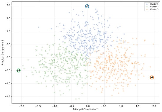
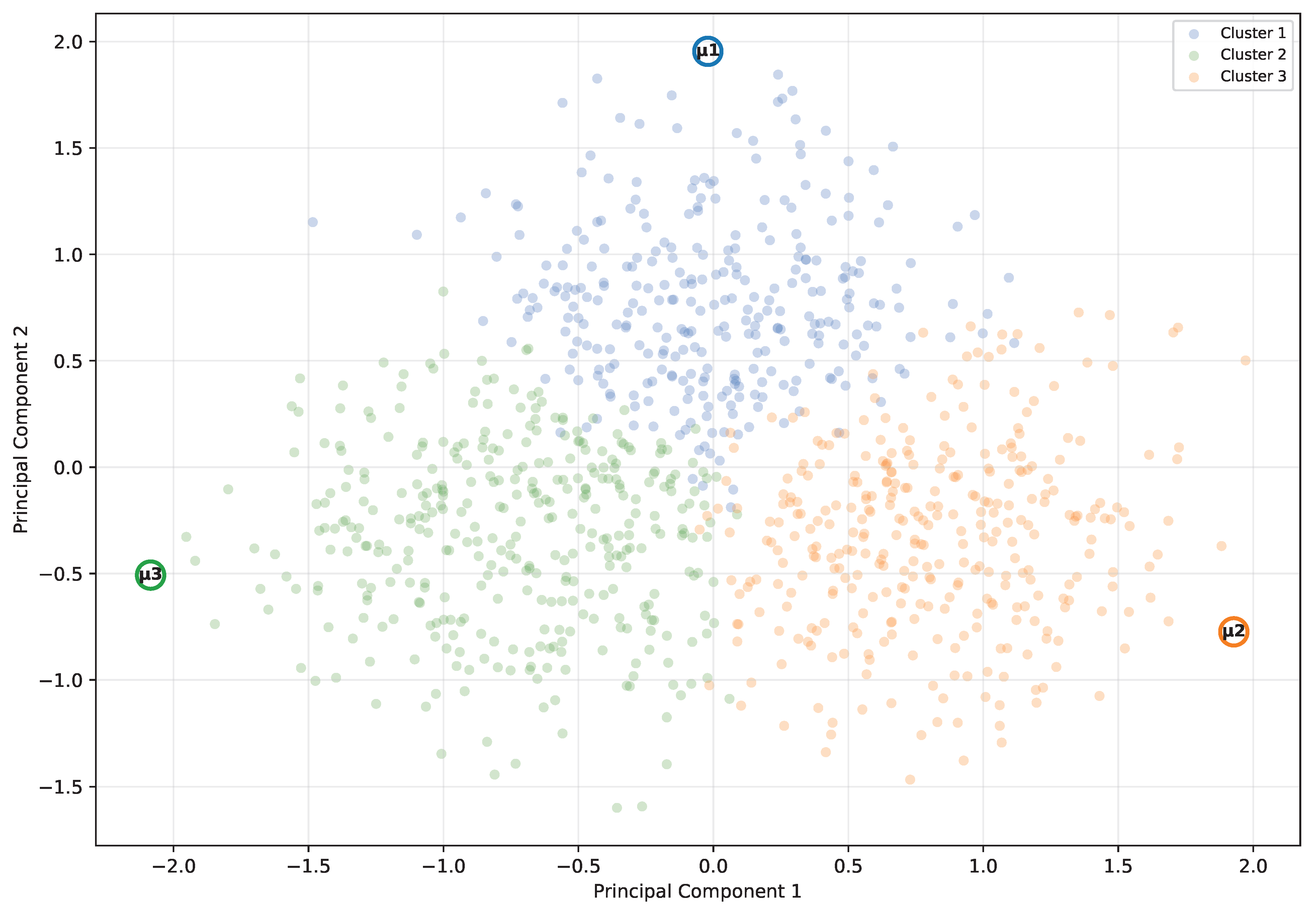
Then the method described in Section 3.1 is applied to the obtained output dataset $\mathcal{Y}=\{Y^1,\dots ,Y^N\}$. The resulting two-dimensional PCA plot is shown in Figure 2.

Figure 2. PCA result.

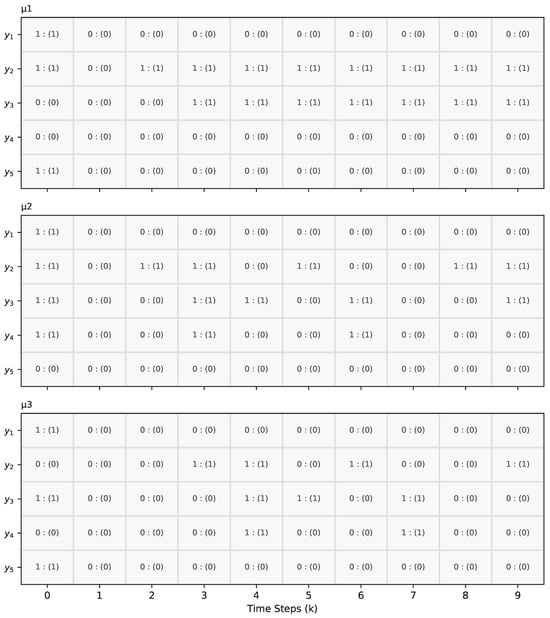
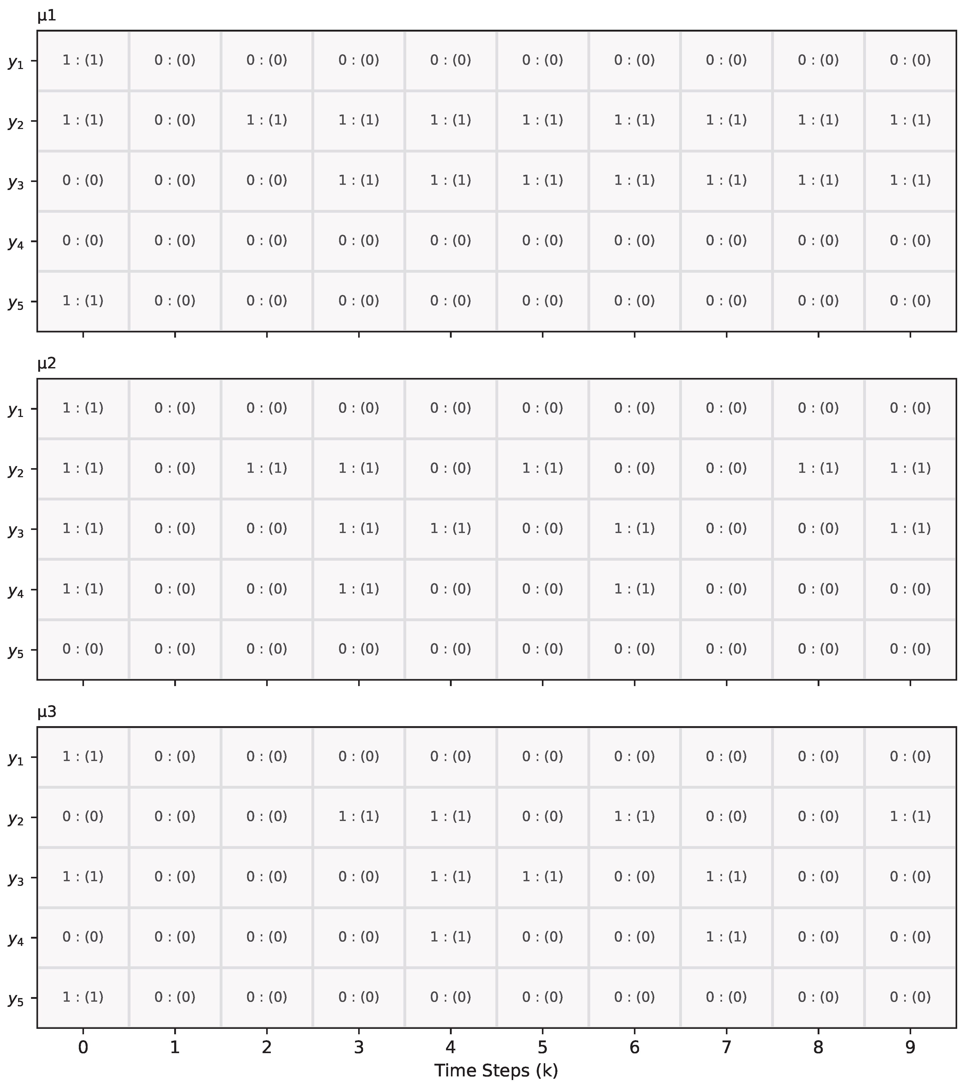
In Figure 2, three clusters with distinct colors can be observed, corresponding to the three candidate initial states ($q=3$) specified in the simulation setup. The cluster centroids are well separated, and the data points show little overlap. This indicates that, despite the presence of noise, K-means clustering clearly distinguishes the output datasets generated from different initial states, which is beneficial for the subsequent reconstruction procedure. The reconstruction method described in Section 3.2 is then applied. The corresponding spatiotemporal discrepancy grid is shown in Figure 3.

Figure 3. Reconstruction result, where $X:\left(Y\right)$ represents that X is the estimated value and Y is the true value.

Figure 3 shows that the reconstructions for all three clusters are successful. The corresponding initial states are obtained as follows:

$$\left\{\begin{array}{cc}\hfill {\mathbf{x}}_0^1& ={[1,1,0,0,1,1,0,1,0]}^{\top },\hfill \\ \hfill {\mathbf{x}}_0^2& ={[1,0,1,0,1,0,0,1,1]}^{\top },\hfill \\ \hfill {\mathbf{x}}_0^3& ={[1,1,1,1,0,0,1,0,1]}^{\top }.\hfill \end{array}\right.$$

(16)

Since all true initial states are correctly matched and identified, the complete evolution of ${\mathcal{F}}_{mc}$ can be obtained. Therefore, the reconstruction is successfully achieved.

For comparison, the measured execution time and traced peak memory usage were as follows: the baseline method required 0.002624 s and 1.155 MB, whereas the proposed method required 0.035039 s and 1.210 MB.

4.2. Sensitivity Experiment

This section evaluates the sensitivity of the proposed method to several parameters and compares its accuracy with that of the baseline. Each experiment is repeated 50 times to account for run-to-run variability, and the mean accuracy is reported.

4.2.1. Noise Level

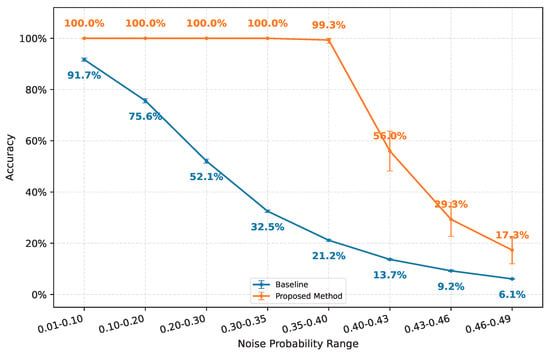
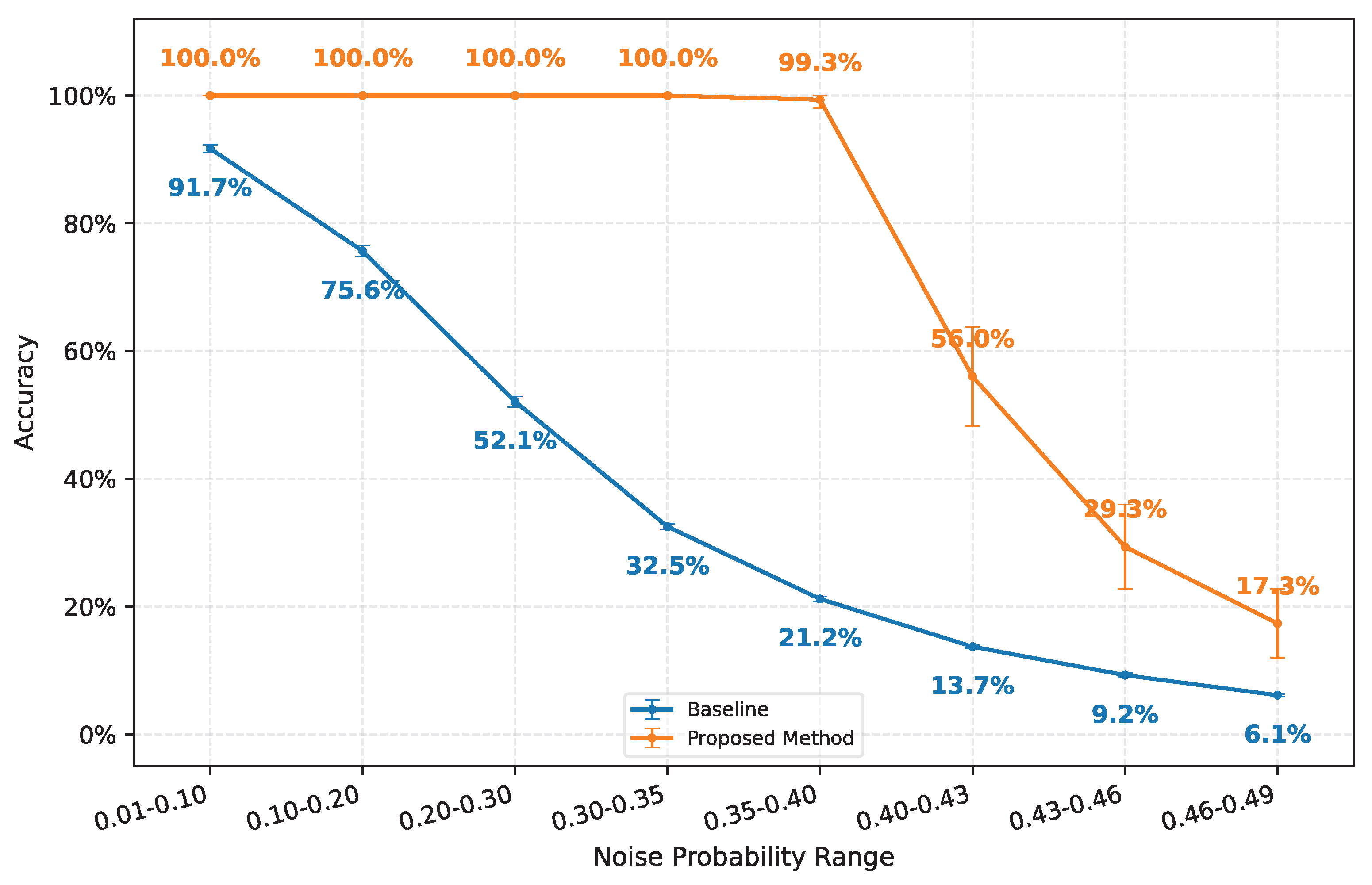
All parameters except the noise probability are held fixed. We consider eight bit-flip probability ranges: $(0.01,0.10)$, $(0.10,0.20)$, $(0.20,0.30)$, $(0.30,0.35)$, $(0.35,0.40)$, $(0.40,0.43)$, $(0.43,0.46)$, and $(0.46,0.49)$. The accuracy comparison is shown in Figure 4.

Figure 4. Accuracy comparison for different noise probability ranges.

Figure 4 shows that the proposed method consistently outperforms the baseline across all tested noise ranges. At the lowest range, $(0.01,0.10)$, the baseline also achieves relatively high accuracy, as direct matching is less affected by noise. As the noise level increases, baseline accuracy declines rapidly, and the largest accuracy gap occurs in the $(0.35,0.40)$ range. Above 0.40, the proposed method’s accuracy also decreases; in the highest tested range, $(0.46,0.49)$, it falls below 20% but remains higher than the baseline. This trend is consistent with Assumption 2: as the noise probability approaches 0.5, the reliability $c_j\left(k\right)$ approaches 0.5, making the true outputs harder to recover by averaging and thresholding.

4.2.2. Number of Candidate Initial States

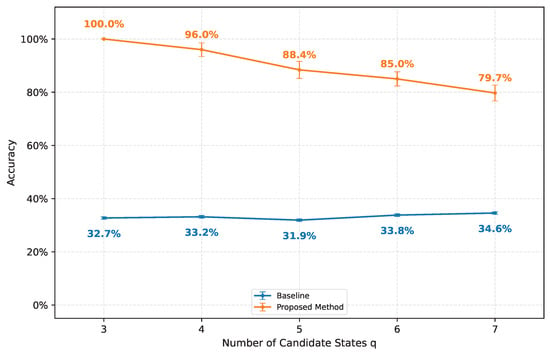
In this experiment, all parameters except the number of candidate initial states, q, are held fixed. We consider $q\in \{3,4,5,6,7\}$; the accuracy comparison is shown in Figure 5.

Figure 5. Accuracy comparison for different numbers of candidate initial states.

Figure 5 shows that the proposed method outperforms the baseline for all five tested values of q. The baseline accuracy varies little with q, remaining within approximately 30–35%. This is consistent with the preceding noise-level results for the $(0.30,0.35)$ range, which is used here. By contrast, the proposed method’s accuracy decreases as q increases. With the measured outputs and time horizon held fixed, a larger candidate set may include initial states with more similar output trajectories, making them harder to distinguish and reducing clustering and reconstruction accuracy. This trend indicates a limitation when candidate states are not sufficiently distinguishable from the available outputs and motivates an observability or trajectory-separability check before reconstruction. However, this experiment alone does not establish a loss of formal observability.

4.2.3. Time Horizon

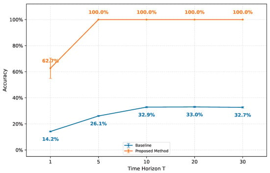
In this experiment, all parameters except the time horizon T are held fixed. We consider $T\in \{1,5,10,20,30\}$; the accuracy results are shown in Figure 6.

Figure 6. Accuracy comparison for different time horizons.

Figure 6 shows that accuracy is particularly sensitive to the time horizon for short horizons, especially as T increases from 1 to 5. For $T\ge 10$, the baseline accuracy stabilizes near 33%, consistent with its performance in the preceding experiments under the same bit-flip probability range, $(0.30,0.35)$. Thus, increasing T beyond 10 yields little further improvement for the baseline under these conditions. In contrast, the proposed method reaches 100% accuracy at $T=5$, achieving complete reconstruction with a shorter horizon in this experiment. This suggests that, under the tested conditions, the proposed method is less constrained by the horizon length than direct matching. Nevertheless, the horizon required for accurate reconstruction depends on the BN structure and the number q of candidate initial states; characterizing this dependence is left for future work.

5. Conclusions

In this paper, we investigated the reconstruction of BNs under probabilistic observation noise using only input–output datasets. The proposed framework first groups noisy output sequences into q clusters by K-means, with PCA used to visualize their separability. It then removes the noise within each cluster and matches the reconstructed trajectories with a noise-free reference library using the Hamming distance, thereby identifying the corresponding initial states in ${\mathcal{X}}_0$.

The numerical examples demonstrated that the method can accurately reconstruct trajectories when sufficient output information is available. They also showed that the reconstruction performance is affected by the number and selection of output variables, the noise level, and the size of the candidate initial-state set.

The results further revealed a limitation of the K-means-based approach when the number q of candidate states becomes large. In this case, Boolean trajectories may become densely distributed in the feature space, causing clusters to overlap and reducing reconstruction accuracy.

In future work, we will address this scalability issue by introducing deep clustering methods. Autoencoders may be used to learn nonlinear low-dimensional representations of trajectories, while contrastive learning could enhance the separation between different state trajectories and improve robustness to noise.

References

- Kitano, H. Systems biology: A brief overview. Science 2002, 295, 1662–1664. [Google Scholar] [CrossRef] [Scilit] [PubMed]
- Wolkenhauer, O.; Mesarović, M. Feedback dynamics and cell function: Why systems biology is called systems biology. Mol. Biosyst. 2005, 1, 14–16. [Google Scholar] [CrossRef] [Scilit] [PubMed]
- Chuang, H.Y.; Hofree, M.; Ideker, T. A decade of systems biology. Annu. Rev. Cell Dev. Biol. 2010, 26, 721–744. [Google Scholar] [CrossRef] [Scilit] [PubMed]
- Chen, B.S.; Wu, C.C. Systems biology as an integrated platform for bioinformatics, systems synthetic biology, and systems metabolic engineering. Cells 2013, 2, 635–688. [Google Scholar] [CrossRef] [Scilit] [PubMed]
- Hecker, M.; Lambeck, S.; Toepfer, S.; Van Someren, E.; Guthke, R. Gene regulatory network inference: Data integration in dynamic models—A review. Biosystems 2009, 96, 86–103. [Google Scholar] [CrossRef] [Scilit] [PubMed]
- Li, H.; Wang, N.; Gong, P.; Perkins, E.J.; Zhang, C. Learning the structure of gene regulatory networks from time series gene expression data. BMC Genom. 2011, 12, S13. [Google Scholar] [CrossRef] [Scilit] [PubMed]
- Li, L.; Sun, L.; Chen, G.; Wong, C.W.; Ching, W.K.; Liu, Z.P. LogBTF: Gene regulatory network inference using Boolean threshold network model from single-cell gene expression data. Bioinformatics 2023, 39, btad256. [Google Scholar] [CrossRef] [Scilit] [PubMed]
- Kadelka, C.; Butrie, T.M.; Hilton, E.; Kinseth, J.; Schmidt, A.; Serdarevic, H. A meta-analysis of Boolean network models reveals design principles of gene regulatory networks. Sci. Adv. 2024, 10, eadj0822. [Google Scholar] [CrossRef] [Scilit] [PubMed]
- Kauffman, S. Homeostasis and differentiation in random genetic control networks. Nature 1969, 224, 177–178. [Google Scholar] [CrossRef] [Scilit] [PubMed]
- De Jong, H. Modeling and simulation of genetic regulatory systems: A literature review. J. Comput. Biol. 2002, 9, 67–103. [Google Scholar] [CrossRef] [Scilit] [PubMed]
- Albert, R.; Othmer, H.G. The topology of the regulatory interactions predicts the expression pattern of the segment polarity genes in Drosophila melanogaster. J. Theor. Biol. 2003, 223, 1–18. [Google Scholar] [CrossRef] [Scilit] [PubMed]
- Beneš, N.; Brim, L.; Kadlecaj, J.; Pastva, S.; Šafránek, D. Exploring attractor bifurcations in Boolean networks. BMC Bioinform. 2022, 23, 173. [Google Scholar] [CrossRef] [Scilit] [PubMed]
- Trinh, V.G.; Park, K.H.; Pastva, S.; Rozum, J.C. Mapping the attractor landscape of Boolean networks with biobalm. Bioinformatics 2025, 41, btaf280. [Google Scholar] [CrossRef] [Scilit] [PubMed]
- Liu, Y.; Wang, L.; Yang, Y.; Wu, Z.G. Minimal observability of Boolean control networks. Syst. Control Lett. 2022, 163, 105204. [Google Scholar] [CrossRef] [Scilit]
- Zhang, K. A survey on observability of Boolean control networks. Control Theory Technol. 2023, 21, 115–147. [Google Scholar] [CrossRef] [Scilit]
- Kobayashi, K.; Wu, Y. Optimal reconstruction of noisy dynamics and selection probabilities in Boolean networks. Automatica 2022, 136, 110094. [Google Scholar] [CrossRef] [Scilit]
- Chen, X.; Kobayashi, K.; Yamashita, Y. On Reconstruction of Boolean Networks Using Input-Output Data Sets. In Proceedings of the 2025 IEEE 14th Global Conference on Consumer Electronics (GCCE), Osaka, Japan, 23–26 September 2025; pp. 215–216. [Google Scholar]
- Billingsley, P. Probability and Measure, 3rd ed.; Wiley: Hoboken, NJ, USA, 1995. [Google Scholar]
- Hoeffding, W. Probability Inequalities for Sums of Bounded Random Variables. J. Am. Stat. Assoc. 1963, 58, 13–30. [Google Scholar] [CrossRef]
- Fauré, A.; Naldi, A.; Chaouiya, C.; Thieffry, D. Dynamical analysis of a generic Boolean model for the control of the mammalian cell cycle. Bioinformatics 2006, 22, e124–e131. [Google Scholar] [CrossRef] [Scilit]
Disclaimer/Publisher’s Note: The statements, opinions and data contained in all publications are solely those of the individual author(s) and contributor(s) and not of MDPI and/or the editor(s). MDPI and/or the editor(s) disclaim responsibility for any injury to people or property resulting from any ideas, methods, instructions or products referred to in the content. |
© 2026 by the authors. Licensee MDPI, Basel, Switzerland. This article is an open access article distributed under the terms and conditions of the Creative Commons Attribution (CC BY) license.