


Abstract
Reconstruction of cultural-heritage fragments requires selecting suitable edge correspondences in the absence of geometric and visual information. LLMFR is a new hybrid framework that integrates large language model-based evaluation with an estimation of distribution algorithm (EDA) and Monte Carlo Tree Search (MCTS). EDA samples candidate fracture edges based on an adaptive probability model, and then MCTS performs a search in the sampled candidate edges set for assemblies. A large language model evaluates the semantic consistency of the reconstructed images. Its global and local feedback updates the EDA probability model for subsequent iterations. We evaluated LLMFR qualitatively on synthetically degraded images and quantitatively on RePAIR under edge damage, pattern staining, fragment loss, and combined damage. The geometry-based GGM achieved the highest mean scores under pattern staining. LLMFR achieved higher mean adjacency F1 and correct placement rate than the geometry-based and texture-based baselines under edge damage, fragment loss, and combined damage.
1. Introduction
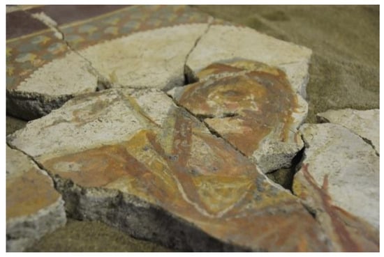
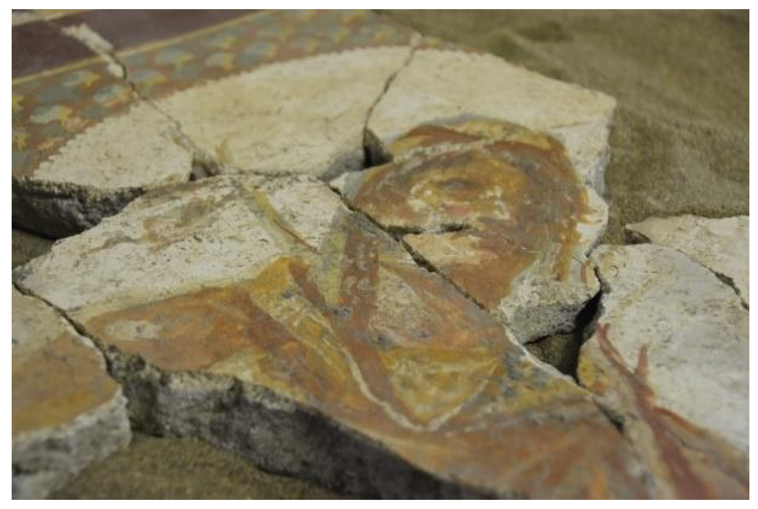
Cultural-heritage objects are generally referred to as scrolls, calligraphic works, paintings, ancient documents, ceramics, murals, etc. [1]. Fluctuations in temperature and humidity, microbial decomposition, geological disasters, and human activities can all produce numerous small, irregularly shaped pieces of these objects that damage their text and pictures [2]. Figure 1 shows painted ceiling fragments from Pompeii [3]. For instance, the individual manuscripts from the Library Cave (Cave 17) of the Dunhuang Mogao Grottoes may have been broken into over a hundred pieces [4]. The edges of these are often abraded, carbonized, or creased, and the surface images may have faded, with color bleeding and staining. There is damage to both the shape and the appearance of the fragments.
Figure 1.
Painted ceiling fragments from Pompeii. Reproduced from Figure 1 of Zuchtriegel et al. [3] under the Creative Commons Attribution License (CC BY).
Conservation specialists have traditionally reconstructed cultural-heritage objects by visual comparison of fragments [5]. They consider the shape of the edges, the connection of surface patterns, and changes in color and texture according to knowledge of the dynasty and art of the object. This approach is suitable for building a reliable model when there are few damaged areas. The number of fragments and the extent of damage increase, and thus reconstruction becomes more difficult. Reconstruction of a single batch of severely fragmented objects will take the specialists several months or years [6].
Automated reconstruction methods are based on fragment geometry or visual content. Geometry-based methods extract contour feature points or approximate contours as polygons, then rank candidate matches according to geometric agreement [7]. These methods work well on preserved edges, but abrasion, chipping, and curling can cause false matches. Visual content-based methods are based on the texture and color of surfaces [8]. They match handcrafted feature points, analyze grayscale continuity, or extract features with deep learning. The effectiveness of the preserved surface pattern is reduced due to pigment oxidation, staining, and damage to the pattern.
From an optimization perspective, fragment reconstruction requires selecting compatible correspondences among irregular fragment edges and assembling the resulting configuration. Edge degradation reduces the geometric information, and staining and fragment loss increase the uncertainty of appearance-based matching. These conditions motivate a search process that combines geometric information with semantic feedback when evaluating candidate assemblies.
LLMFR (Large Language Model Fragment Reconstruction) is a new hybrid combinatorial search method for fragment image reconstruction. Computer Vision methods extract geometric and appearance features from fragment images. An estimation of distribution algorithm (EDA) samples candidate fracture edges from an adaptive probability model, and Monte Carlo Tree Search (MCTS) performs assembly exploration based on these edges. A large language model assesses the semantic coherence of the assembled pictorial patterns. Its global and local feedback updates the EDA probability matrix to guide candidate-edge sampling in the next iteration.
2. Related Work
Fragment reconstruction is a combinatorial optimization problem involving irregularly shaped pieces [9]. Research began with classical jigsaw puzzles and extended to cultural relic restoration and medical image mosaicking [10]. Studies of cultural relic reconstruction can be grouped into geometry-based, computer vision-based, and deep learning-based methods. These methods have limited generalization and need to be adapted to the specific application of the heritage.
Geometry-based methods were one of the first types of fragment reconstruction. Acquire contour features and find the geometric correspondence of corresponding edges [7]. The Douglas–Peucker algorithm is often employed to reduce the number of contours. Fourier Descriptors and Shape Context encode contours as rotation- and translation-invariant feature vectors, and then, by minimizing the feature distance, select the candidate-edge pair. These methods work well when edges are preserved, but abrasion, carbonization-induced chipping, and curling can disrupt matching. Some studies divide contours into local areas and screen candidate pairs according to the segment agreement [2]. This reduces the impact of local defects on the overall match, but severe edge degradation remains a limitation.
Degradation of edge geometry can be addressed by matching color and texture of adjacent areas. Visual Content-Based Methods Extract Surface Features and Evaluate Continuity of Candidate Joins. Early methods used Speeded-Up Robust Features (SURF), Oriented FAST and Rotated BRIEF (ORB), and Random Sample Consensus (RANSAC) for geometric transformation estimation. They created accurate reconstructions of the parts with different surface features [11]. For murals and paintings with abundant color information, color-based methods compare distributions across adjacent edges and can help when texture is weak [12]. A study of Dunhuang manuscript reconstruction based on physical, structural and semantic features: grayscale similarity, contour geometry and textual structure. The Tower of Hanoi model was used for global reconstruction optimization and then tested on a small fragment dataset [13]. Fading pigments and stains are also defects because they have altered the original color of the product [12].
Deep learning methods learn features and matching rules from data. Deepzzle is used to classify the relative positions of fragments, and Dijkstra’s shortest-path algorithm is applied to build a global assembly [14]. It can fill in the missing parts and is relatively immune to light-edge erosion. Generative Models and Large Language Models (LLMs) have also been used for reconstruction. A system based on SGRGAN learns the style and composition of Song Dynasty paintings to consistently inpaint missing areas in that style [15]. The inpainted content can help to find the fragment and reduce the effect of damaged boundaries on matching. LLMCO4MR is a cardinality-constrained combinatorial optimization model for reconstruction [16]. A neural combinatorial solver is used to generate candidate matches, and a multimodal large language model is employed to add semantic knowledge from historical documents. The framework improves semantic plausibility and performs well on the Dunhuang manuscript fragment dataset. Most of these models have been trained on artificial data and lack cross-domain generalization [17]. They also lack effective global constraints and can accumulate reconstruction errors [12].
ReassembleNet learns contour keypoints and estimates fragment poses via diffusion to reconstruct irregular fragments and incorporates geometric and texture information for 2D fresco reconstruction [18]. By contrast, LLMFR uses a pretrained multimodal evaluator to direct EDA sampling and MCTS assembly without the need for additional task-specific training. Related Concerns Also Arise Outside Fragment Reconstruction. Gao et al. study resilient hierarchical control for digital-twin cloud–edge collaboration under non-ideal communication conditions [19] and Liu et al. have used progressive graph convolution with spatio-temporal self-attention for traffic flow prediction [20]. These studies have drawn attention to graph structure and degraded information. Probabilistic candidate sampling and graph-based search are used in conjunction with semantic evaluation.
Robustness and transfer across scenarios remain limitations in the reconstruction of ancient scrolls, calligraphic works, and paintings [17]. Serious damage to the edges, missing fragments, and differences in artistic style make reconstruction more difficult. Some learning-based methods also need task-specific training data that are difficult to obtain for damaged cultural heritage [18]. LLMFR meets the above requirements by combining adaptive candidate-edge sampling with EDA, MCTS-based assembly search, and guidance of discrete matching decisions by language model-based semantic feedback.
3. System Model
Fragment reconstruction involves discrete decisions about which edges are candidate fracture edges and which pairs should be matched. The number of possible combinations is directly proportional to the number of fragments and candidate edges. Geometric congruence and the continuity of surface patterns provide support for the above decisions but can also be disrupted. LLMFR solves the combinatorial search problem using probabilistic candidate selection and tree search with semantic evaluation.
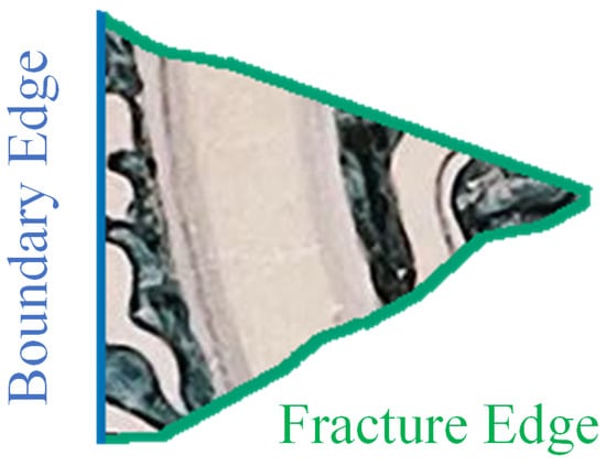
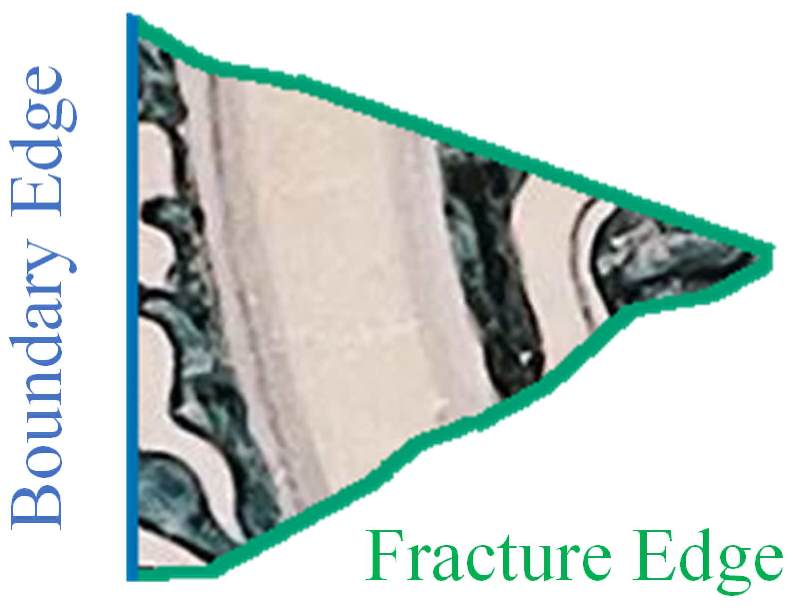
Fragment contours contain exterior boundary segments and fracture segments created by fragmentation. In the two-dimensional domain, reconstruction estimates the relative poses of individual fragments; at the combinatorial level, it selects candidate correspondences between fracture segments. Figure 2 illustrates these two types of segments. A fragment adjacency graph records the topological structure induced by the selected correspondences. In the dual edge space, by contrast, the reconstruction process becomes the task of establishing correct one-to-one correspondences between fracture edges to achieve combinatorial restoration. It can be formally proven that, within a topologically connected space, the one-to-one pairing of fracture edges in the edge space is mathematically equivalent to the combinatorial optimization of relative fragment poses in the two-dimensional spatial domain. Accordingly, the fragment reconstruction problem can be reduced to the core task of identifying the correct one-to-one matching between fracture edges.
Figure 2.
An example of boundary edges and fracture edges in a fragment.
Theorem 1.
Let be a connected simple graph whose vertices represent fragments and whose edges represent their adjacency relations induced by correct fracture-edge correspondences. If G is isomorphic to neither nor , its line graph determines G up to graph isomorphism among connected simple graphs.
Proof.
We use the Whitney Line Graph Isomorphism Theorem [21] to relate the isomorphism of line graphs to that of their underlying graphs.
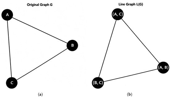
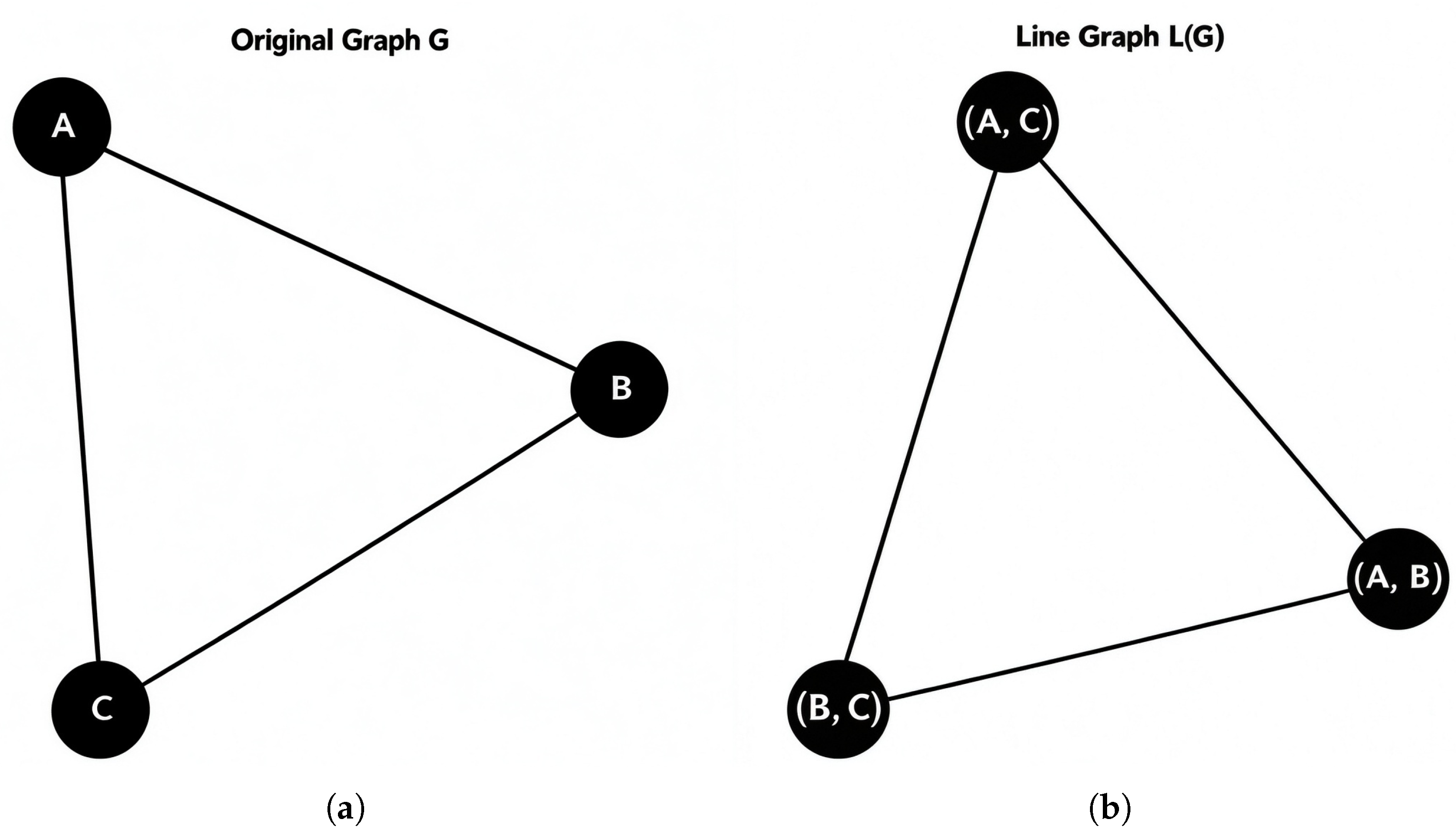
For an arbitrary simple graph , its line graph (see Figure 3) is defined as follows:
Figure 3.
A schematic diagram of G and . (a) The original graph G, with vertices A, B, and C representing fragments. (b) The line graph , with each vertex labeled by the endpoints of the corresponding edge in G.
- The vertex set of is identical to the edge set of G, i.e., ;
- Two vertices are adjacent in if and only if the corresponding edges and share a common endpoint in G.
Let G and H be connected simple graphs. Then with the unique exception of the graph pair : where denotes the complete graph on n vertices, and denotes the complete bipartite claw graph with vertex partitions of size 1 and 3. □
Except for the ambiguity between and , a connected simple graph is determined up to isomorphism by its line graph. The Whitney Line Graph Isomorphism Theorem thus confirms that establishing a correct one-to-one correspondence between fracture edges is sufficient to achieve a complete combinatorial reconstruction of the fragments. By reframing the fragment reconstruction problem as the search for a topological one-to-one mapping of fracture edges, this framework circumvents the need for conventional matching criteria such as edge geometric congruence and surface pattern continuity, thereby enabling reliable reconstruction even in scenarios with missing fragments and severe structural degradation.
Finding the correct fracture-edge correspondences remains a difficult combinatorial problem. The reconstruction workflow has three stages: distinguish fracture edges from boundary edges, pair the matching fracture edges, and assemble the fragments from the verified correspondences.
4. Fragment Reconstruction Algorithm
4.1. Fragment Image Extraction
Contour extraction, polygonal approximation, and edge segmentation turn the raw fragment contours into ordered edge segments with geometric attributes [22,23]. Each segment is given a fragment ID and a local edge sequence number for boundary-edge and fracture-edge classification.
4.1.1. Initial Extraction of Closed Contours
A foreground mask is first obtained from the alpha channel of four-channel fragment images or from grayscale conversion followed by fixed-threshold binarization of three-channel images [22]. Extract the outer contour of the mask, and if its area exceeds the lower bound, keep this contour. This retrieval mode excludes internal hole contours. The implementation uses alpha and grayscale thresholds of 128 and 127, respectively, and a minimum contour area of 100 square pixels.
Let the outer contour of the k-th fragment be represented by , where is the number of contour points and gives the pixel coordinates of the t-th point. The points follow the order of the extracted closed contour. Clockwise ordering is imposed on the vertices obtained during subsequent polygonal approximation.
4.1.2. Polygonal Approximation and Edge Segmentation
The continuous contour is discretized using Douglas–Peucker polygonal approximation, with a tolerance expressed as a percentage of the contour perimeter and a default value of 1%. The resulting vertices are ordered clockwise in image coordinates. Each consecutive vertex pair, including the last-to-first pair, defines a polygon edge. The segments are indexed sequentially around the contour to form the fragment’s local edge set:
where is the i-th edge segment of the k-th fragment. Thus, the neighbors of the adjacent areas are still disconnected. It is a local sequence that does not need a spatial arrangement of the edge sets of the fragments.
4.2. EDA-Based Edge Classification
Incremental EDA with an independent Bernoulli probability model selects candidate fracture edges [24]. Each edge has a selection probability. Sampling and coverage repair generate candidate sets, and feedback from the preceding reconstruction cycle updates the probabilities for the next iteration.
Let denote all fragment edges, including boundary and fracture edges, and let K denote the candidate fracture edge set at the current iteration. For each , define , with indicating inclusion in the initial candidate sample and indicating exclusion. Coverage repair, described below, produces the final candidate set K. Inclusion in this set does not establish that an edge is a true fracture edge.
Each edge is assigned a probability , where t denotes the iteration. For a fixed iteration t, we abbreviate as . Initial sampling assumes independence of edges and obtains the factorized Bernoulli model:
The initial probability is set to for every edge segment, assigning equal prior probabilities to the two classes in the absence of domain-specific prior knowledge.
Each edge is sampled independently according to the current probability model:
where is the indicator function and is uniformly distributed over . The selected edges form the set of candidate fracture edges.
A coverage-repair heuristic is then used. If the fragment does not have selected edges, then the edge with the highest probability will be selected. If the total is still less than , where F is the number of fragments, the unselected edges will be added in descending order of probability until the threshold is reached or no more edges are available. This process generates the set of active candidate fracture edges K.
4.3. MCTS-Based Fragment Reconstruction
MCTS identifies a one-to-one fracture-edge correspondence for optimization of fragment connectivity [25]. These pairs determine the topology of the fragment-level reconstruction, and fragment positions and poses are set in assembly.
4.3.1. Search States and Tree Nodes
EDA supplies the candidate fracture edge set. Each candidate edge is a search unit identified by its parent fragment and local edge index. At each MCTS node, records the current pairings: contains the candidate fracture edges, and contains valid edge pairings used for reconstruction. The initial state has an empty .
A sequence of fracture-edge pair operations is required for the path from the root to a search node. Further along in the Path, the confirmed pairs and local assemblies are more numerous.
4.3.2. Reconstruction Performance Evaluation System
At each MCTS node, only whether the fracture edges are connected is recorded in . Overlap errors, rotation angles, displacement, or contour-matching measures are not stored. Evaluation at this time is therefore limited to topology. A fast scoring system is constructed based on four indicators: the number of connected components C, the number of isolated fragments , the number of over-adjacent fragments , and the number of triangular cycles .
- C: The number of connected components, corresponding to disconnected blocks in the final reconstruction graph. The ideal value, , represents a single integrated structure. Larger values of C indicate a more fragmented reconstruction.
- : The number of degree-zero nodes, representing fragments with no adjacent neighbors. The ideal value is ; larger values of indicate more extensive matching failure.
- : A higher degree does not necessarily indicate a better reconstruction, since a physical fragment can be adjacent to only a limited number of neighbors, typically four to six. Unusually high degrees suggest excessive false matches. An empirical upper bound is therefore specified according to fragment type. For thin planar fragments, including paper, murals, and pottery shards, the maximum adjacency is . The number of fragments satisfying is denoted by .
- : Mutual connections among three fragments form a triangular cycle. Such cycles can occur in valid fragment assemblies and are not, by themselves, evidence of a false match. The current scoring function uses their count, , as a heuristic penalty to discourage premature closed local clusters during search. This heuristic does not explicitly prohibit triangular states, but it may penalize valid clusters.
The comprehensive scoring function S is then defined as:
4.3.3. MCTS
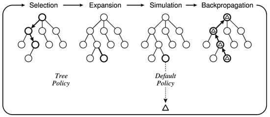
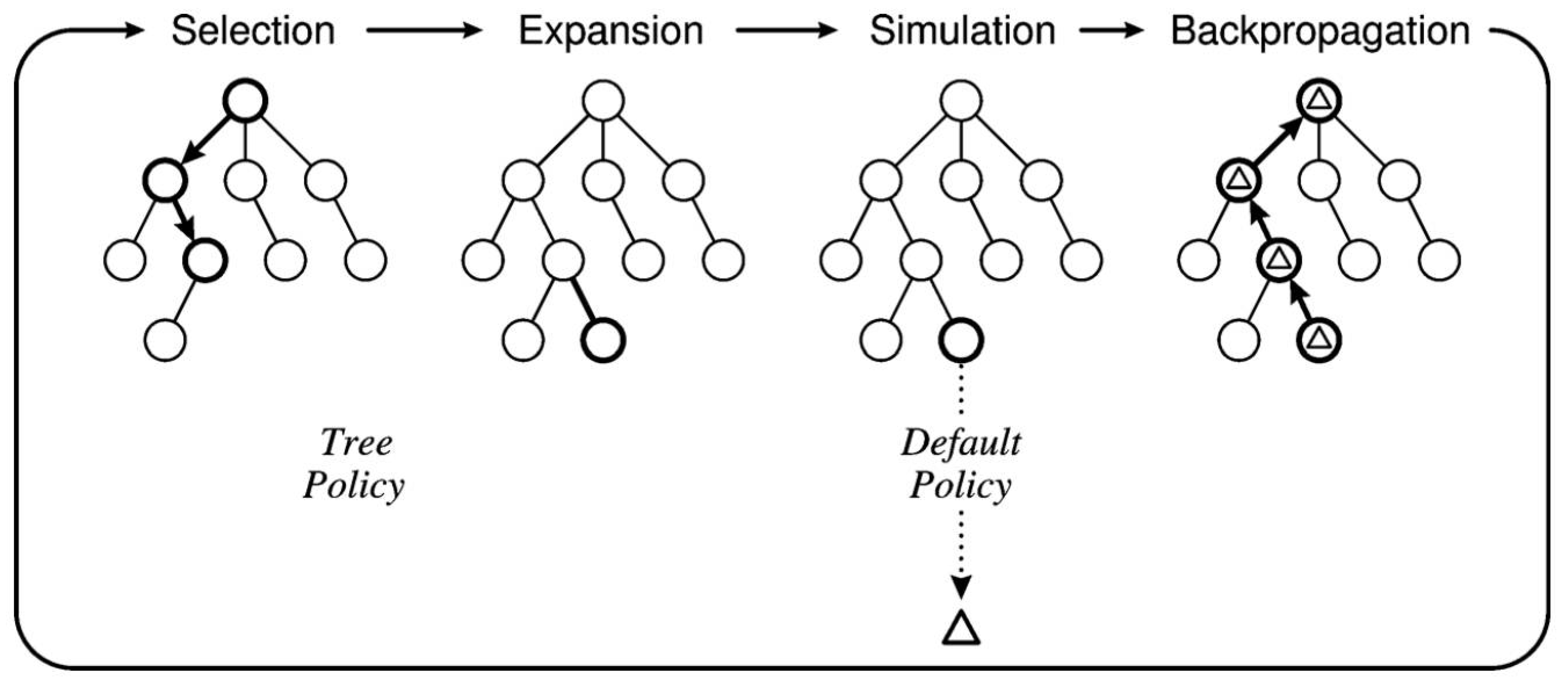
Run MCTS for 1000 tree-search iterations on each pair of fracture-edge decisions and set the exploration constant to 1.414. Each iteration starts at the root and selects the next node from the current reconstruction. Select based on the average reward of past rollouts and explore less frequently visited nodes. Figure 4 shows the MCTS search of consecutive fracture-edge pairs.
Figure 4.
Flowchart of MCTS.
If the search finds a non-terminal node that has not been fully explored, a valid pair can be obtained from its unused fracture edges. The resulting state is a child node. Sibling nodes represent alternative pairings from the same state, and tree depth is the number of pairing decisions.
After expansion, a random simulation rollout is initiated from the newly created child node. Valid fracture-edge pairings are successively added until no further pairing is available or the score differs from 1 by no more than . No maximum rollout length is imposed in the present implementation. Repeated rollouts estimate how a local pairing decision may affect the eventual reconstruction and provide an empirical basis for comparing alternative pairing sequences.
A high-reward pair will not be connected further and will be left alone. A low-reward pair may be suitable for the final assembly. MCTS employs rollouts to approximate the effects on the final reconstruction topology.
The final topological score S of each rollout is backpropagated to the root as the reward, updating the visit count and cumulative reward of every node on the path. These statistics estimate the outcomes of subsequent pairing decisions from each state.
After the prescribed number of tree-search iterations, the root child with the highest average simulation reward determines the pairing selected for the current reconstruction stage. This pairing is applied to the current state, and a new search tree is constructed from the updated state to determine the next pairing. The sequence of pairing decisions continues until no legal pairing remains or the score is within the same tolerance of 1.
When the search terminates, the fracture-edge indices are mapped to their corresponding fragment identifiers and local edge indices, yielding the selected fracture edge correspondences.
4.4. Fragment Reconstruction
Assembly estimates the rotations and translations of a common coordinate system with respect to the one-to-one fracture-edge correspondences [17,22]. Voronoi fragments are created before the reconstruction loop. Contour vertices and edge lengths are extracted once and reused in the assembly. Then, cross-correspondence is performed to extend the rigid-body constraint graph of fragment adjacency via Breadth-First Search (BFS). Alpha blending integrates the aligned fragment layers to construct the reconstructed image.
4.4.1. Voronoi Fragment Generation
Two-dimensional seed points are sampled uniformly over the fragment image. For each pixel position, Euclidean distances to all seeds are computed, and the pixel is assigned to the Voronoi region of the nearest seed. A predefined probability determines whether boundary perturbation is applied to each region, rather than whether individual pixels are deleted. When perturbation is enabled, an eight-neighborhood test identifies the boundary pixels, from which a subset is sampled without replacement for removal. The number of removals is the result of dividing the boundary-pixel count by a random integer from 3 to 8 and taking the floor, with a minimum of 1 for a non-empty boundary. Next, crop the region based on its bounding box and add its mask to the alpha channel to obtain an RGBA image of only the target fragment.
4.4.2. Geometric Feature Extraction
First, read the fragment image and then select the largest outer contour as the representation of the fragment. Douglas–Peucker polygonal approximation reduces this contour to a finite vertex set. The signed area determines the orientation, and the vertex sequence is reversed when necessary to ensure clockwise ordering in image coordinates. Geometry is extracted once before the iterative reconstruction loop, and then assembly reuses the stored vertices and edge lengths.
4.4.3. Edge Correspondence Verification
Three checks precede reconstruction. First, all edge indices are checked against their valid ranges. Second, compare the corresponding edge lengths and, if the difference between the longest and shortest edges is more than 10% of the shortest length, then consider the match invalid. Third, fragment-level BFS verifies that the correspondence graph contains a single connected component. If this graph is disconnected, only the component containing fragment 0 can be placed, and connectivity verification is needed before reconstruction.
4.4.4. BFS Rigid Pose Propagation
Edge Correspondences are converted into Fragment Adjacency Relations. The fixed position of the reference fragment is at , and no rotation of BFS is employed. When a constraint connects a placed fragment A to an unplaced fragment B, the rotation and translation of B are determined by the corresponding edge of B, and then B is marked as visited. Pose propagation is a coordinate transformation, using a discrete search over 72 rotation angles with edge midpoint alignment.
4.4.5. Alpha Blending
Based on the determined positions, the axis-aligned extent of each fragment image can be obtained from its half-diagonal length. Increase the Margin of the four-channel canvas on all sides to 100 px. Rotate and position each fragment according to the calculated location in the canvas.
4.5. LLM-Based Reconstruction Scoring
Scores based primarily on contour fitting and texture similarity may provide limited evidence when geometric or appearance cues are degraded. The proposed scoring framework supplements these cues with large language model-based assessments of visual and textual coherence. Archaeological context also provides specific conditions for the application of cultural heritage. The purpose of this assessment is to select candidates, not to verify the historical accuracy of the assembly.
The scoring framework combines physical features, semantic features, and archaeological knowledge through an LLM [16,26]. The reconstruction workflow does not introduce a separate task-specific model training stage; it uses a pretrained language model for evaluation.
4.5.1. Multi-Dimensional Scoring Framework
The scoring framework comprises three levels: basic physical properties, semantic features, and archaeological knowledge. Each Level has two score indices. The above are used to conduct all-around and localized evaluations in the search.
- Basic Physical Layer: Match the geometric shape, materials, and craftsmanship consistency assessment to ensure the feasibility of reconstruction.
- Semantic Feature Layer: Continuity of decorative patterns and coherence of text evaluate the semantic consistency of the reconstruction. LLMs contribute most directly at this level.
- Archaeological Knowledge Layer: Assess the archaeological plausibility of chronological and cultural compatibility and formal-contextual rationality. This level assesses formal compatibility rather than performing rigorous archaeological restoration validation.
4.5.2. Multimodal Scoring Scheme
The LLM assigns scores across the six dimensions and combines them into comprehensive and local assessments. It solves the problem of conflicting geometry and semantics in setting the evaluation score.
The assessment proceeds through the following stages:
- Preliminary Screening Layer: Information from the basic physical layer is used to rule out obviously incorrect local assessments and obtain an overall judgment of reconstruction performance.
- Semantic Verification Layer: Determine the continuity of decorative patterns and coherence of text; identify logical errors in pattern logic and inconsistencies in text sequence.
- Knowledge Validation Layer: Archaeological plausibility is checked with the existing metadata and contextual information of artifacts. Unsupported chronological or cultural judgments are listed as unknown and are not considered verification of historical accuracy.
- Comprehensive Evaluation Layer: The LLM integrates the preceding assessments with domain knowledge to generate a comprehensive score . It also identifies local strengths and prominent errors. denotes the local score assigned to the correspondence between fragment edges m and n at iteration t.
The following are the prompt JSON scoring rules: All assessment criteria scores, the overall score , and the valid local correspondence scores are integers ranging from 0 to 10, and a higher score indicates stronger support for the reconstruction or correspondence. Unassessable criteria are shown as null, and unassessable correspondences are not added to the local-score list. Comprehensive and local scores are used directly in the probability-update formulas without normalization.
SYSTEM
You evaluate a candidate reconstruction of cultural-heritage fragments.
Use only the supplied image, identifiers, and metadata. No ground-truth
assembly is provided. Do not invent historical facts or claim access to
an external database. State uncertainty explicitly.
USER
Evaluate the attached assembly.
Fragment IDs: {{fragment_ids}}
Matched pairs [fragment_a, edge_a, fragment_b, edge_b]:
{{matched_pairs}}
Verified artifact metadata: {{metadata_or_none}}
Identifier labels do not imply that a match is correct.
Assess:
1. Visible geometric compatibility.
2. Visible material and craftsmanship consistency.
3. Decorative-pattern continuity.
4. Text continuity where legible text exists.
5. Chronological/cultural compatibility where metadata supports it.
6. Formal/contextual plausibility.
Score each applicable criterion using an integer from 0 to 10:
0 = strong visible contradiction; 5 = ambiguous or mixed evidence;
10 = strong visible support. Use intermediate integers for intermediate
levels of support. Use null for unassessable criteria, not zero.
Return global_score as one integer from 0 to 10 on the same scale,
considering only applicable criteria. Explain how the applicable
criteria support this overall score in their reason fields.
Identify up to three strongest and three weakest assessable supplied
matched pairs. Return exact pair IDs, integer local scores from 0 to 10
on the same support scale, strength/weakness labels, and evidence-based
reasons. Do not invent IDs. Omit unassessable pairs; use an empty
local_scores list if no pair is assessable.
Apply the same scoring scale independently to every reconstruction.
Do not normalize scores or output fractional scores.
Return JSON only with these keys:
{"criteria":[{"name":"...","score":null,"reason":"..."}],
"global_score":5,
"local_scores":[{"pair":["f1","e1","f2","e2"],"score":8,
"type":"strength","reason":"..."}],
"uncertainty":"...","failure_modes":[],"limitations":[]}
The shown values illustrate the schema, not the evaluation result.
Before saving the feedback, check that the score is a whole number between 0 and 10, and confirm that the local correspondence identifier matches the provided one. The valid global and local scores are added to the update formula in their original 0–10 scale without division by 10 or other normalization.
4.6. Probability Model Matrix Update for EDA
Before iteration t, the probability model is updated using feedback from the reconstruction produced by MCTS at iteration . The update applies to the used-edge set . Edges with high-scoring or low-scoring correspondences use their local scores ; edges without an explicit local assessment use the comprehensive reconstruction score . Candidate edges are then resampled from the updated probability model.
For edges without an explicit local assessment, the update before iteration uses . The baseline is , and the first iteration uses . For an edge assigned a valid local correspondence assessment from iteration , the feedback signal is , comparing the local score with the comprehensive score of the same reconstruction. Both scores use the same integer 0–10 scale, so and are computed directly in score points without normalization. The formulas below describe the comprehensive-score update; the corresponding local signal is substituted for edges with a local assessment. Edge-selection probabilities and correspondence scores describe different quantities.
4.6.1. Adaptive Learning Rate
Feedback is applied only to the edges used in the reconstruction selected at iteration , denoted by , rather than to the entire candidate set K. The update computes from before candidate sampling at iteration t. No update is applied if the used-edge set is empty or is zero within an absolute tolerance of .
An increase in the evaluation score provides a positive update signal for the fracture edges used in the preceding reconstruction, without establishing a causal contribution for each edge. Their selection probabilities are therefore increased, whereas a decrease in the score reduces these probabilities. Restricting the update to used edges avoids assigning global feedback to candidates that did not contribute to the final reconstruction.
The adaptive learning rate is defined as:
where and . The term is a monotonic increasing saturation function. Small changes in the score result in a small adjustment, and only large changes increase the learning rate to 0.6, thereby enhancing the impact of significant feedback on the probability model.
4.6.2. Probability Model Matrix
If is empty, all probabilities remain unchanged. For each used edge, a zero applicable feedback signal leaves that edge’s probability unchanged. For a nonzero comprehensive-score signal, the binary learning target is defined below; for an edge with a local assessment, its local signal replaces in both the learning rate and the target. Thus, the learning rate and target are evaluated per edge when local feedback is used.
For each used edge e with a nonzero feedback signal from the reconstruction at iteration , exponential smoothing updates its selection probability:
Equivalently,
For , the target is , giving which increases the probability towards 1. For , the target is , giving which decreases the probability towards 0.
To prevent premature convergence to the deterministic values 0 and 1, the updated probabilities are restricted to the interval :
This clipping operation maintains a minimum degree of exploration. An edge that has repeatedly received negative evaluations retains at least a 5% probability of being sampled in a subsequent iteration. Similarly, repeated positive evaluations do not make its selection deterministic.
The probabilities of edges outside are left unchanged:
4.7. Overall Workflow
Figure 5 shows the LLMFR workflow. Computer vision methods extract contour geometry and surface pictorial information. EDA samples candidate fracture edges, and MCTS searches for assemblies using those candidates. The LLM evaluates the reconstructed visual content and provides global and local feedback to update the EDA probability matrix for the next iteration.
Figure 5.
Algorithm flowchart of LLMFR.
5. Experiments
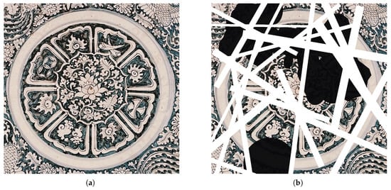
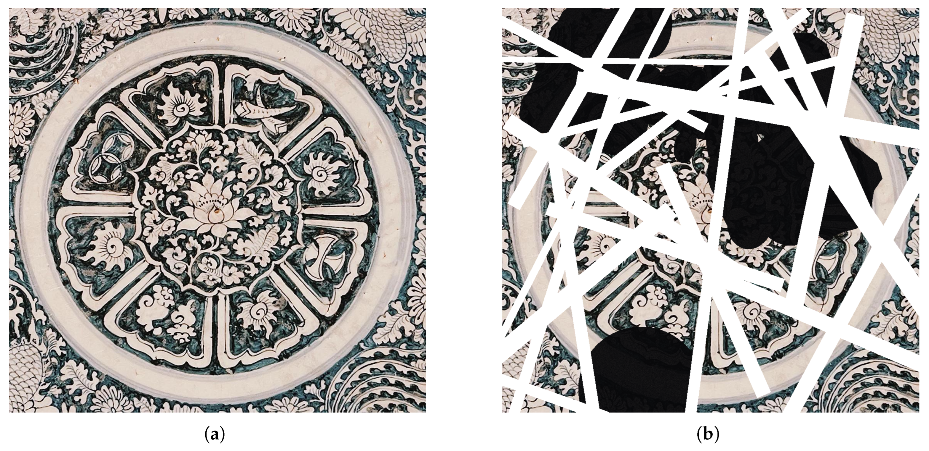
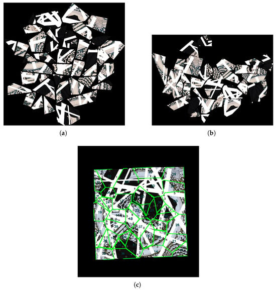
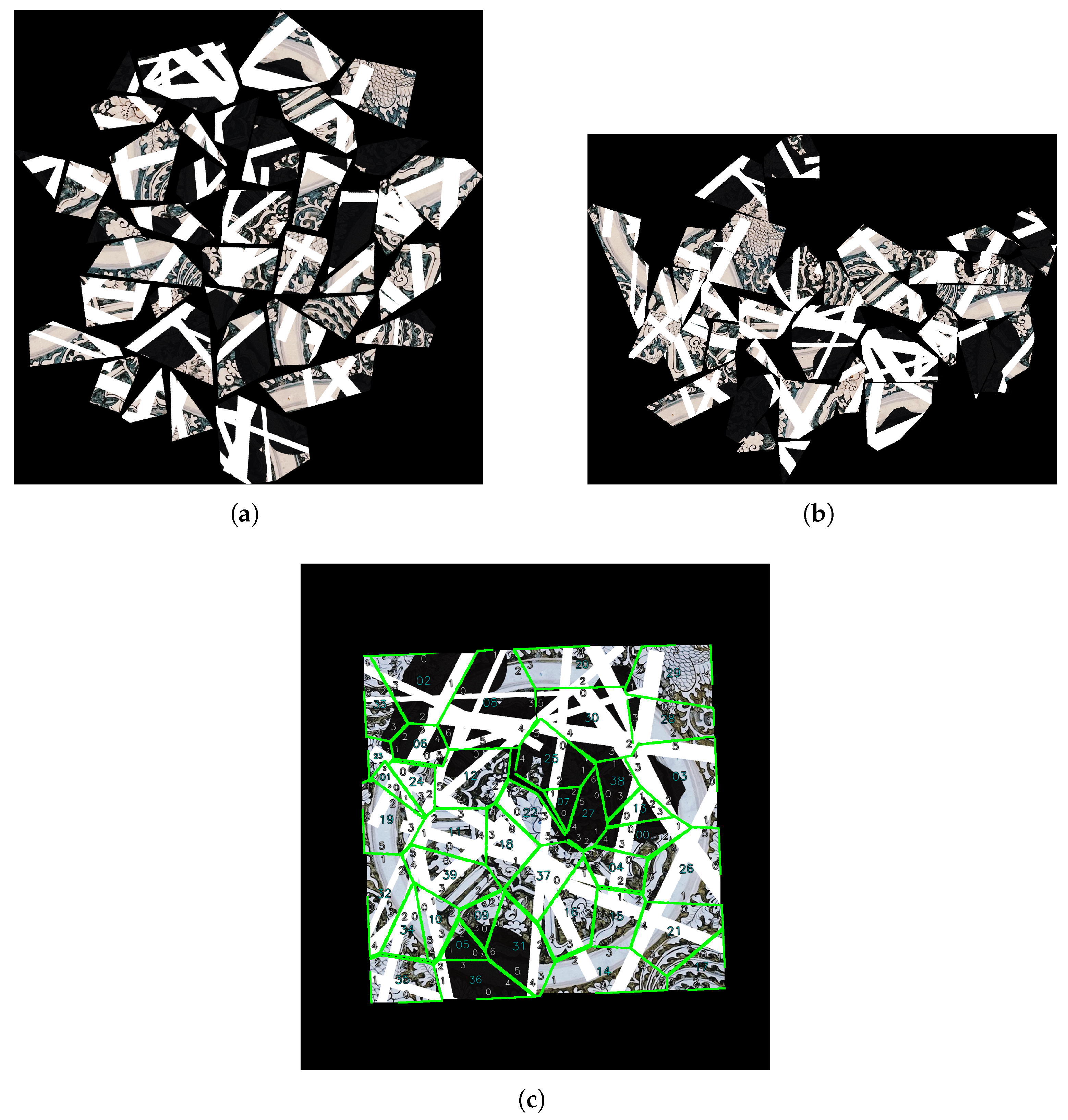
After edge damage, pattern staining, fragment loss, and combined damage were observed in LLMFR. We artificially reduced the original images by adding complex visual information for qualitative comparison with geometry-based and texture-based baselines. Figure 6 shows the untreated reference sample and the sample after artificial pattern staining.
Figure 6.
(a) Intact baseline sample. (b) The same sample with simulated pattern staining.
We used greedy geometric matching (GGM) and pattern texture stitching (PTS) as baselines. GGM reconstructs fragments by aligning their contours through iterative nearest-point computation [17]. PTS reconstructs fragments by matching texture features [2].
Experiments used an Intel Core i5-14600KF processor, an NVIDIA RTX 3090 graphics card, and 32 GB of RAM. The software environment comprised Python 3.7.9 and OpenCV 4.13.0. The original language model-based evaluation was described as using ChatGPT 5.6 Sol [27,28,29]. The exact model version and inference settings of the original scorer are given in Table 1 and the alternative model versions are identified in Section 5.5.1.
Table 1.
Model version and inference settings of the original ChatGPT scorer.
RePAIR was used for the quantitative evaluation [17]. It contains digitized fresco fragments from Pompeii, including irregular fractures, erosion, and missing pieces. Expert-assembled groups provide reference configurations. We used version 2 of the public dataset (https://doi.org/10.5281/zenodo.15800029), specifically the 2D_SOLVED.zip archive, which provides fragment images and reference transformations for two-dimensional reconstruction. Groups were included if they contained at least two fragments with readable images and valid reference poses. Open-discovery fragments without verified solutions were not counted in the quantitative score. Ground-truth configurations were used only for evaluation and were not provided to the reconstruction method or the LLM scorer.
Table 2 shows the size strata of the evaluated RePAIR subset before the additional removal. Use the same test set for the four damage conditions and repeat each test case five times. The total number of subsets is 100, and among them, 40 have 2–5 fragments, 40 have 6–10 fragments, and 20 have 11–44 fragments. Edge damage and pattern staining do not destroy all the pieces. Repeated damage versions of the same group are not considered new independent source groups.
Table 2.
Composition of the evaluated RePAIR subset before additional removal.
The four conditions below were constructed by applying additional controlled perturbations to the selected RePAIR groups rather than using official RePAIR damage categories. The settings were 20% additional boundary-pixel removal, 40% artificial surface staining, and removal of 15–20% of the supplied fragments. The combined-damage condition applied all three perturbations. Fragment-removal counts were rounded to integers, so the realized removal fractions could differ from the target proportions. Damage added was measured relative to the released input, and natural deterioration has not occurred. All the methods used the same perturbed input for all the test cases. The figures in this section are synthetic qualitative examples, and Table 3, Table 4, Table 5 and Table 6 present the quantitative results of RePAIR.
Table 3.
Quantitative results on RePAIR under edge damage (20% additional boundary-pixel removal). Values are means ± standard deviations across group averages. An upward arrow indicates that higher values are better.
Table 4.
Quantitative results on RePAIR under pattern staining (40% artificial surface staining). Values are means ± standard deviations across group averages. An upward arrow indicates that higher values are better.
Table 5.
Quantitative results on RePAIR under fragment loss. Values are means ± standard deviations across group averages. An upward arrow indicates that higher values are better.
Table 6.
Quantitative results on RePAIR under combined damage. Values are means ± standard deviations across group averages. An upward arrow indicates that higher values are better.
Adjacency F1 was computed from sets of unordered fragment pairs. Let denote the set of predicted fragment pairs and the set of ground-truth adjacent fragment pairs. Each unordered pair was included only once, regardless of the number of matched edge segments between the two fragments. Predicted pairs were obtained from the final fragment correspondences used for assembly. The numbers of true positives, false positives, and false negatives were defined as , , and , respectively. For a nonzero denominator, adjacency F1 is
For the fragment-loss experiments, the ground-truth adjacency graph was restricted to the retained fragments. Fragments without the corresponding pieces were not employed as ground-truth neighbors. Due to the proximity of the fragments, matching of individual edge segments is not required for this index.
The correct placement rate was computed as the percentage of all input fragments whose reference-centroid positions and orientations agreed with their ground-truth poses within the evaluation tolerances. Reference centroids and fragment areas were computed from the released masks before additional degradation so that artificial erosion did not change the evaluation landmarks. The rotation tolerance was 5°, using the smallest angular difference modulo 360°. Unplaced fragments were counted as incorrect.
For each condition, the scores of the five reconstruction runs in a test instance and all instances in a RePAIR group were averaged. Table 3, Table 4, Table 5 and Table 6 report the mean ± standard deviation of the group averages, with equal weight for each group. Adjacency F1 is between 0 and 1, and the proportion of correctly placed items is shown as a percentage.
5.1. Edge Breakage Test Scenario
Edge damage is common in cultural-heritage fragments and arises mainly from burial-environment erosion and mechanical impacts during excavation. Abrasion and exfoliation along fragment edges degrade the geometry of the original fracture surfaces. We simulated edge weathering by randomly deleting edge pixels at an erosion rate of 20%, defined as the ratio of damaged edge pixels to the total number of edge pixels in a fragment.
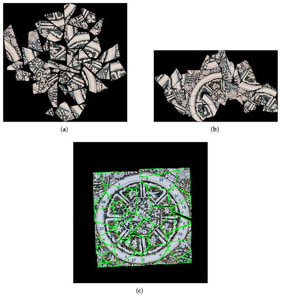
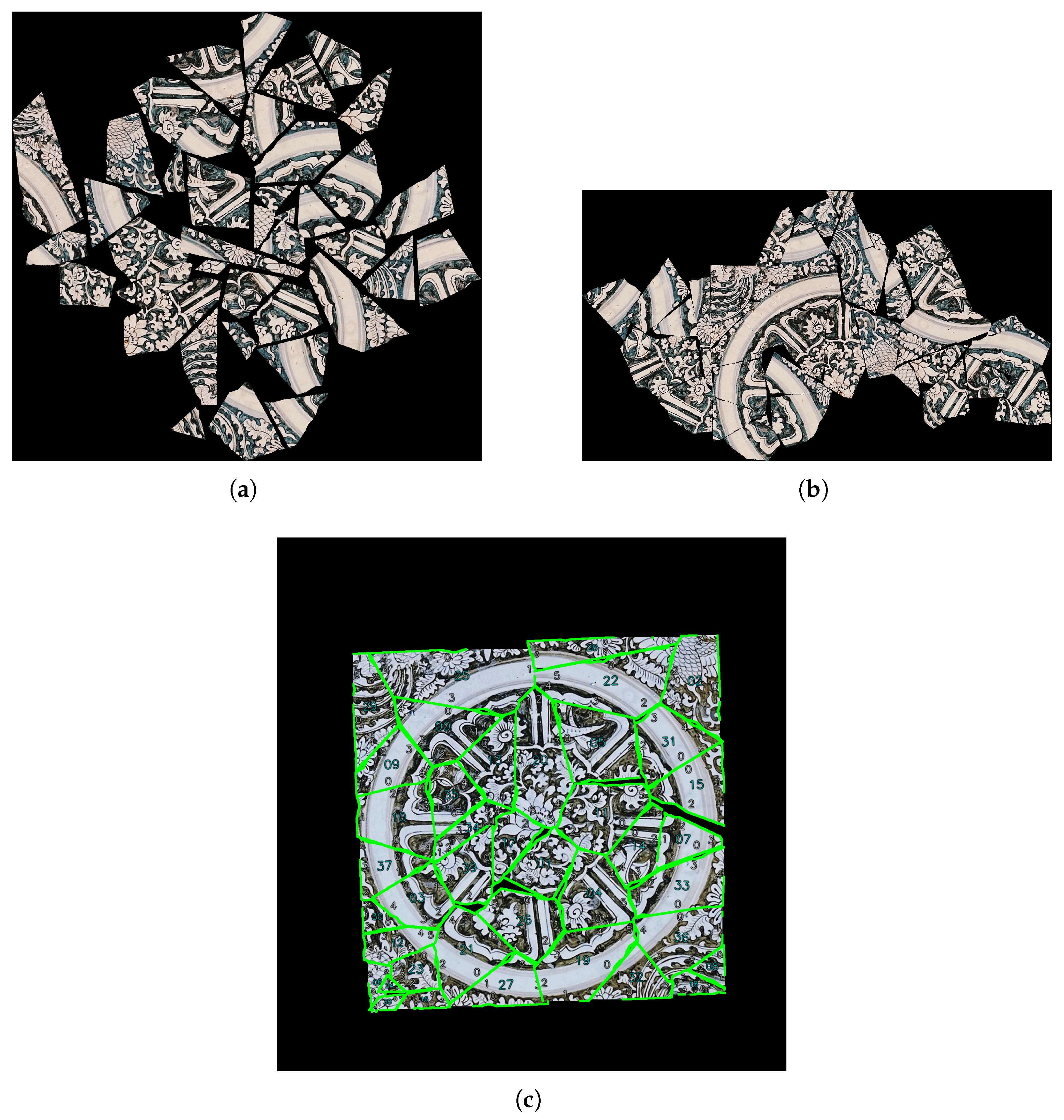
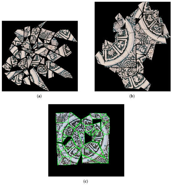
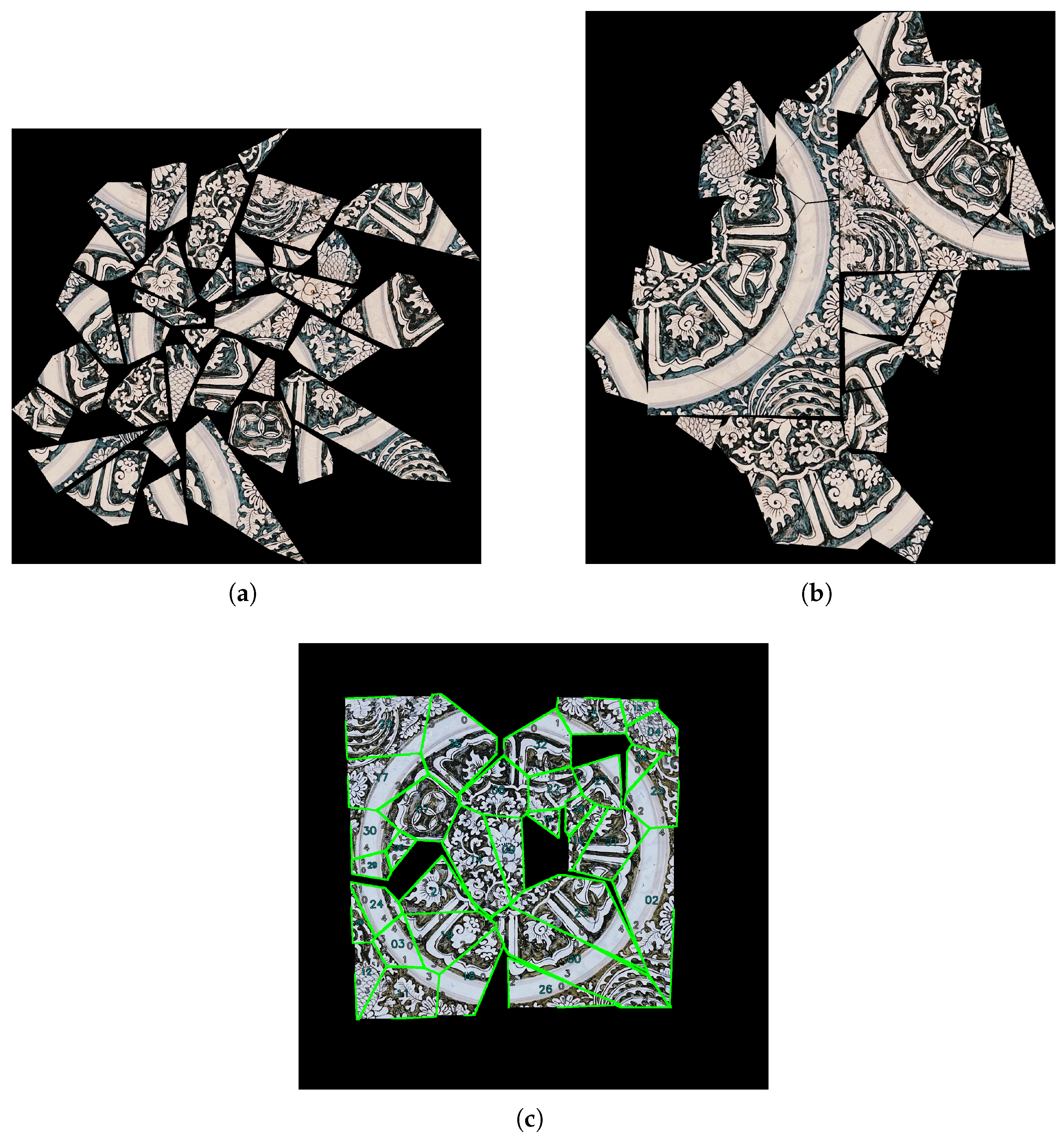
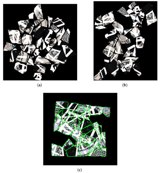
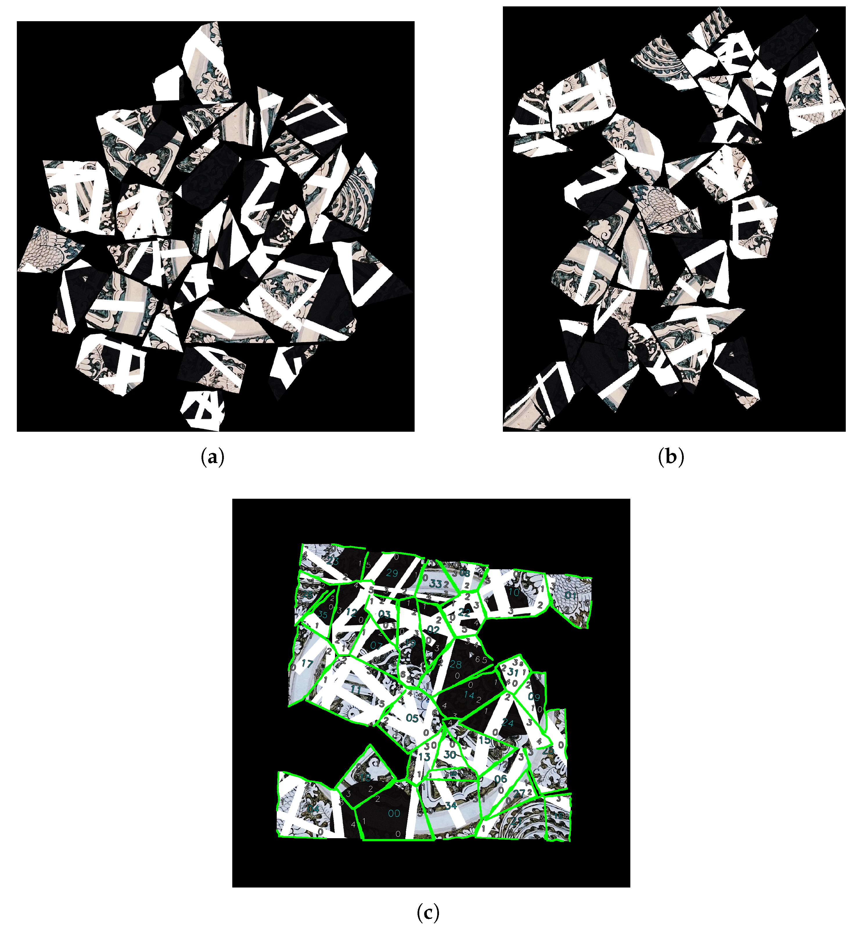
As shown in the synthetic example of Figure 7, LLMFR appears to keep the fragment arrangement better than both baselines. In panel (c) of Figure 7, Figure 8, Figure 9 and Figure 10, the cyan numbers identify individual fragments, and the smaller numbers along each fragment’s outline identify its edge segments, numbered separately for each fragment. It also had the highest mean adjacency F1 and correct placement rate among the three methods for RePAIR with edge damage (Table 3). Its core advantage lies in its capacity to effectively distinguish original fracture edges from weathered boundary edges via the EDA module, which filters out noise interference from damaged edges and restricts geometric matching exclusively to valid fracture edges. Combined with the global search optimization capability of MCTS, this mechanism significantly mitigates the adverse impact of edge fracture on reconstruction accuracy.
Figure 7.
Qualitative reconstruction results for a synthetic edge-damage example. (a) GGM. (b) PTS. (c) LLMFR.
Figure 8.
Qualitative reconstruction results for a synthetic pattern-staining example. (a) GGM. (b) PTS. (c) LLMFR.
Figure 9.
Qualitative reconstruction results for a synthetic fragment-loss example. (a) GGM. (b) PTS. (c) LLMFR.
Figure 10.
Qualitative reconstruction results for a synthetic combined-damage example. (a) GGM. (b) PTS. (c) LLMFR.
5.2. Pattern-Staining Test Scenario
Pigment exfoliation, surface calcification, and staining can hide or change the original surface pattern and texture. Black blocks and white scratch strips are used to create pattern stains. Set the proportion of the stained area to 40% of the surface of the fragment and count the number of stained pixels divided by the total number of surface pixels.
In the synthetic staining example in Figure 8, LLMFR shows better continuity of visible pictorial content than the baselines. On the evaluated RePAIR groups, however, GGM achieved the highest mean adjacency F1 and correct placement rate under pattern staining (Table 4). The added surface staining does not change the fracture-edge shape directly and may be responsible for the enhanced performance of GGM in this case.
5.3. Fragment-Loss Test Scenario
Historical deterioration and the loss of individual fragments leave gaps in an assembly, reducing the available matching context and increasing the risk of false matches. We artificially introduced fragmentation loss by random deletion. The proportion of target removal from the original fragment count was 15–20%, and the number of removals was rounded to an integer.
Figure 9 shows a synthetic fragment-loss example. On RePAIR, LLMFR achieved the highest mean adjacency F1 and correct placement rate among the three evaluated methods under fragment loss (Table 5). Conventional algorithms depend on local adjacent feature matching; missing fragments break the continuity of matching chains, resulting in a substantial number of misaligned pairings. The proposed LLMFR algorithm integrates the MCTS strategy, which effectively narrows the matching search space even in the presence of incomplete fragments.
5.4. Compound Interference Test Scenario
There are many types of damage to cultural-heritage fragments. To investigate the combined effects, edge damage, pattern staining, and fragment loss were introduced simultaneously.
Figure 10 shows a synthetic combined-damage example. On Repair, LLMFR achieved a higher mean adjacency F1 and correct placement rate than both baselines in the presence of damage (Table 6). For LLMFR under combined damage, the adjacency F1 score is 0.48, and the correct placement rate is only 37%. Erosion reduces the geometric constraints; Staining damages semantic continuity; Missing fragments lose intermediate adjacency evidence. An incorrect match may result in a false adjacent constraint and increase the reconstruction error. These reasons accumulate misalignment during the iteration process and lead to failure. In the future, experts will review the uncertain or conflicting assessments and correct the feedback to update the probability.
5.5. Sensitivity Analysis and Limited Ablation
The sensitivity and limited-ablation study used the 40-fragment synthetic edge-damage case in Figure 7, and the set condition of 20% boundary-pixel damage was employed. We studied the scorer substitution and removal of adaptive probability updates.
5.5.1. Scorer Substitution
The original scorer was compared with Gemini 3.1 Pro and DeepSeek-V4.1-Flash using the same visual inputs, prompt, fragment and edge identifiers, and metadata. Table 1 reports the configuration of the original ChatGPT scorer. The JSON prompt and integer 0–10 scoring protocol are specified in Section 4.5.2. Global and local scores are used directly in the update formulas without normalization, as described in Section 4.6.
Table 7 shows the scorer-substitution results on the 40-fragment synthetic edge-damage case by ChatGPT, Gemini, and DeepSeek. It can be seen that different models have little impact.
Table 7.
Scorer-substitution results on the 40-fragment synthetic edge-damage case in Figure 7.
5.5.2. Repeated Scoring of Identical Input
The fixed image in Figure 7a, corresponding to the GGM output, was scored ten times without rerunning reconstruction. ChatGPT 5.6 Sol was used for all ten calls, with no conversation history shared between requests. Table 8 summarizes all ten global-score records, with a mean of 3.60 and a sample standard deviation of 0.5. This indicates that the fluctuation of repeated scoring is relatively small.
Table 8.
Repeated scoring of the fixed GGM reconstruction in Figure 7a.
5.5.3. Fixed-Probability Ablation
The fixed-probability variant sets for every edge and every iteration, disabling both global and local feedback updates to the EDA model while retaining the other reconstruction and selection settings. It was run five times using the same ChatGPT scorer and paired reconstruction seeds as the full method. Table 9 shows the fixed-probability results. The mean adjacency F1 and the mean correct placement of this variant were 0.40 and 39%, respectively; those of the full ChatGPT method were 0.85 and 85% (Table 7). The corresponding decreases were 0.45 F1 and 46 percentage points. Under fixed-probability conditions, LLMFR cannot effectively identify fracture edges, causing the reconstruction process to approximate random combinations and resulting in very poor performance.
Table 9.
Fixed-probability ablation on the 40-fragment synthetic edge-damage case in Figure 7.
5.6. Computational Cost and Reproducibility
External LLM calls are distinct from the 1000 internal MCTS iterations performed per pairing decision. Table 10 reports approximate resource totals for one complete reconstruction of the 40-fragment synthetic edge-damage case in Figure 7.
Table 10.
Approximate resource totals for one complete reconstruction of the 40-fragment synthetic edge-damage case in Figure 7.
6. Conclusions
LLMFR combines EDA-based candidate-edge sampling, MCTS-based assembly search, and language model-based semantic evaluation. Global and local feedback from the language model updates the probability model used to sample edges for subsequent reconstructions. We evaluated the framework on synthetic examples and RePAIR under edge damage, pattern staining, fragment loss, and combined damage. LLMFR achieved the highest mean adjacency F1 and correct placement rate under edge damage, fragment loss, and combined damage, while GGM achieved the highest mean scores under pattern staining. Substantial placement errors remained under combined damage. Further work should test broader fragment collections and damage levels, isolate the contributions of individual components, and assess computational cost and sensitivity to the LLM scorer. Meanwhile, incorporating expert human intervention into the iterative process to promptly correct errors will lead to more effective repairs.
Author Contributions
Methodology, J.Y.; validation, X.S.; investigation, J.Y.; writing—original draft preparation, J.Y.; writing—review and editing, Z.H. All authors have read and agreed to the published version of the manuscript.
Funding
This research received no external funding.
Institutional Review Board Statement
Not applicable.
Informed Consent Statement
Not applicable.
Data Availability Statement
The RePAIR dataset used for the quantitative evaluation is publicly available at https://doi.org/10.5281/zenodo.15800029 (version 2).
Acknowledgments
The authors thank the editors and reviewers for their contributions to the manuscript.
Conflicts of Interest
The authors declare no conflicts of interest.
Abbreviations
The following abbreviations are used in this manuscript:
| LLM | large language model |
| MCTS | Monte Carlo Tree Search |
| EDA | Estimation of Distribution Algorithm |
| LLMFR | Large Language Model Fragment Reconstruction |
| SURF | Speeded-Up Robust Features |
| ORB | Oriented FAST and Rotated BRIEF |
| RANSAC | Random Sample Consensus |
| GGM | greedy geometric matching |
| PTS | pattern texture stitching |
References
- Nuri, A.; Ismayil, Z.; Babayeva, M.; Guliyev, A.; Rzayeva, F.; Shiraliyeva, G.; Jahangirli, T. Artistic Expressions as Vehicles of Cultural Memory: Bridging Identity, Heritage, and Intercultural Understanding. J. Ethn. Cult. Stud. 2025, 12, 258–275. [Google Scholar] [CrossRef] [Scilit] [PubMed]
- Derech, N.; Tal, A.; Shimshoni, I. Solving archaeological puzzles. Pattern Recognit. 2021, 119, 108065. [Google Scholar] [CrossRef] [Scilit]
- Zuchtriegel, G.; Brunetto, M.A.; Gravina, E.; Napolitano, M.C.; Ricciardi, F.S.; Zambrano, A.; Khoroshiltseva, M.; Palmieri, L.; Pelillo, M.; Vascon, S.; et al. The RePAIR Project: Datasets for archaeological and restoration studies in Pompeii. In Proceedings of the Digital Heritage International Congress, Siena, Italy, 8–13 September 2025. [Google Scholar] [CrossRef]
- Xu, H. Determining the Original Appearances of the Scrolls from the Dunhuang Library Cave Based on Their Inventory Records. J. Zhejiang Univ. 2023, 53, 86–103. [Google Scholar]
- Fang, L.; Han, B.; Bi, M.; Wang, L.; Wang, D. DCAF-GAN: Enhancing historical landscape restoration with dual-branch feature extraction and attention fusion. PLoS ONE 2025, 20, e0334532. [Google Scholar] [CrossRef] [Scilit] [PubMed]
- Wang, H.; Zang, Y.; Liang, F.; Dong, Z.; Fan, H.; Yang, B. A Probabilistic Method for Fractured Cultural Relics Automatic Reassembly. J. Comput. Cult. Herit. 2021, 14, 5. [Google Scholar] [CrossRef] [Scilit]
- Rasheed, N.A.; Nordin, M.J. Reconstruction algorithm for archaeological fragments using slope features. ETRI J. 2020, 42, 420–432. [Google Scholar] [CrossRef] [Scilit]
- Eslami, D.; Di Angelo, L.; Di Stefano, P.; Guardiani, E. A Semi-Automatic Reconstruction of Archaeological Pottery Fragments from 2D Images Using Wavelet Transformation. Heritage 2021, 4, 76–90. [Google Scholar] [CrossRef] [Scilit]
- Barbieri, L.; Fuoco, F.; Bruno, F.; Muzzupappa, M. Exhibit supports for sandstone artifacts designed through topology optimization and additive manufacturing techniques. J. Cult. Herit. 2022, 55, 329–338. [Google Scholar] [CrossRef] [Scilit]
- Shahar, O.I.; Elkin, G.; Ben-Shahar, O. The Missing GAP: From Solving Square Jigsaw Puzzles to Handling Real World Archaeological Fragments. arXiv 2026, arXiv:2605.12077. [Google Scholar]
- de Lima-Hernandez, R.; Vergauwen, M. A Hybrid Approach to Reassemble Ancient Decorated Block Fragments through a 3D Puzzling Engine. Remote Sens. 2020, 12, 2526. [Google Scholar] [CrossRef] [Scilit]
- Gigilashvili, D.; Lukesova, H.; Gulbrandsen, C.F.; Harijan, A.; Hardeberg, J.Y. Computational techniques for virtual reconstruction of fragmented archaeological textiles. Herit. Sci. 2023, 11, 259. [Google Scholar] [CrossRef] [Scilit]
- Zheng, Y.T.; Li, X.L.; Yin, Z.X.; Gao, G.; Weng, Y. Multi-feature fusion based automatic reconstruction in related to Chinese ancient manuscript fragments of Dunhuang. J. Image Graph. 2023, 28, 2330–2342. [Google Scholar]
- Paumard, M.-M.; Picard, D.; Tabia, H. Deepzzle: Solving visual jigsaw puzzles with deep learning and shortest path optimization. IEEE Trans. Image Process. 2020, 29, 3569–3581. [Google Scholar] [CrossRef] [Scilit] [PubMed]
- Hu, Q.; Huang, W.; Luo, Y.; Cao, R.; Peng, X.; Peng, J.; Fan, J. Sgrgan: Sketch-guided restoration for traditional Chinese landscape paintings. Herit. Sci. 2024, 12, 163. [Google Scholar] [CrossRef] [Scilit]
- Zhang, Y.; Li, H.; Zhang, S.; Wang, R.; He, B.; Dou, H.; Yan, J.; Zhang, Y.; Wu, F. LLMCO4MR: LLMs-aided Neural Combinatorial Optimization for Ancient Manuscript Restoration from Fragments with Case Studies on Dunhuang. In Proceedings of the 18th European Conference on Computer Vision (ECCV 2024); Springer: Cham, Switzerland, 2024; pp. 253–269. [Google Scholar] [CrossRef] [Scilit]
- Tsesmelis, T.; Palmieri, L.; Khoroshiltseva, M.; Islam, A.; Elkin, G.; Shahar, O.I.; Scarpellini, G.; Fiorini, S.; Ohayon, Y.; Alali, N.; et al. Re-assembling the past: The RePAIR dataset and benchmark for real world 2D and 3D puzzle solving. In Advances in Neural Information Processing Systems; Curran Associates, Inc.: Red Hook, NY, USA, 2024; Volume 37, pp. 30076–30105. [Google Scholar]
- Islam, A.; Fiorini, S.; James, S.; Morerio, P.; Del Bue, A. ReassembleNet: Learnable Keypoints and Diffusion for 2D Fresco Reconstruction. In Proceedings of the IEEE/CVF International Conference on Computer Vision, Honolulu, HI, USA, 19–23 October 2025; pp. 9048–9057. [Google Scholar]
- Gao, Y.; Zhu, H.; Zhang, Z.; Wang, Y.; Ai, Q.; Zhu, J. Resilient hierarchical control strategy for digital twin cloud-edge collaboration in multi-energy microgrids under non-ideal communication conditions. Appl. Energy 2026, 424, 128374. [Google Scholar] [CrossRef] [Scilit]
- Liu, C.; Kou, Y.; Wang, S.; Xie, Z.; Su, Y. Research on traffic flow prediction of progressive graph convolutional networks based on spatio-temporal self-attention mechanism. Sci. Rep. 2026, 16, 14112. [Google Scholar] [CrossRef] [Scilit] [PubMed]
- Harary, F. Graph Theory; Addison-Wesley: Reading, MA, USA, 1969; pp. 72–75. [Google Scholar]
- Zheng, Y.; Li, X.; Weng, Y. Reunion helper: An edge matcher for sibling fragment identification of the Dunhuang manuscript. Herit. Sci. 2024, 12, 52. [Google Scholar] [CrossRef] [Scilit]
- Douglas, D.H.; Peucker, T.K. Algorithms for the reduction of the number of points required to represent a digitized line or its caricature. Cartographica 1973, 10, 112–122. [Google Scholar] [CrossRef] [Scilit]
- Mühlenbein, H.; Paass, G. From recombination of genes to the estimation of distributions I. Binary parameters. In Parallel Problem Solving from Nature—PPSN IV; Springer: Berlin, Germany, 1996; pp. 178–187. [Google Scholar]
- Browne, C.B.; Powley, E.; Whitehouse, D.; Lucas, S.M.; Cowling, P.I.; Rohlfshagen, P.; Tavener, S.; Perez, D.; Samothrakis, S.; Colton, S. A survey of Monte Carlo tree search methods. IEEE Trans. Comput. Intell. AI Games 2012, 4, 1–43. [Google Scholar] [CrossRef] [Scilit]
- Brown, T.B.; Mann, B.; Ryder, N.; Subbiah, M.; Kaplan, J.D.; Dhariwal, P.; Neelakantan, A.; Shyam, P.; Sastry, G.; Askell, A.; et al. Language models are few-shot learners. In Advances in Neural Information Processing Systems (NeurIPS 2020); Curran Associates, Inc.: Red Hook, NY, USA, 2020; Volume 33, pp. 1877–1901. [Google Scholar]
- OpenAI. Previewing GPT-5.6 Sol: A Next-Generation Model. Available online: https://openai.com/index/previewing-gpt-5-6-sol/ (accessed on 3 November 2026).
- OpenAI. GPT-5.6: Frontier Intelligence that Scales with your Ambition. Available online: https://openai.com/index/gpt-5-6/ (accessed on 3 November 2026).
- OpenAI. GPT-5.6 System Card. Available online: https://deploymentsafety.openai.com/gpt-5-6/ (accessed on 3 November 2026).



Disclaimer/Publisher’s Note: The statements, opinions and data contained in all publications are solely those of the individual author(s) and contributor(s) and not of MDPI and/or the editor(s). MDPI and/or the editor(s) disclaim responsibility for any injury to people or property resulting from any ideas, methods, instructions or products referred to in the content. |
© 2026 by the authors. Licensee MDPI, Basel, Switzerland. This article is an open access article distributed under the terms and conditions of the Creative Commons Attribution (CC BY) license.