


Abstract
Environmental conditions may provide information relevant to respiratory deterioration in pig barns, but their value beyond recent acoustic observations remains unclear. This study developed a controlled semi-synthetic benchmark to examine when multimodal fusion of irregularly sampled environmental data and recent acoustic observations improves prediction of future respiratory-acoustic activity. Scores were derived from the aSwine dataset using a frozen PANNs representation and a recording-disjoint classifier, which achieved a macro-averaged held-out ROC AUC of 0.695 and average precision of 0.176. Empirical score distributions were incorporated into simulated 42-day sequences containing ammonia, temperature, relative humidity, and carbon dioxide. Eight models and controls were compared over 20 paired repetitions at coupling strengths 0, 2, 4, and 6. History-matched concatenation achieved mean ROC AUCs of 0.496, 0.518, 0.569, and 0.581, compared with 0.519, 0.494, 0.497, and 0.507 for audio-only prediction. Its advantage remained significant after Holm correction only at coupling 6. Time-aware fusion did not consistently outperform history-matched concatenation or its past-history-permuted control. Additional analyses showed that acoustic persistence, history length, generating assumptions, and alert definitions affected model rankings. Event-level evaluation using validation-selected thresholds showed no consistent operational advantage for fusion. These findings remain conditional on the empirical acoustic-score pools and the specified generator. Validation using synchronized real-farm audio, environmental, and veterinary data is needed.
1. Introduction
1.1. Porcine Respiratory Monitoring and Early Acoustic Alerting
Respiratory disorders constitute a major health and production concern in pig farming. They are associated with reduced welfare and growth performance, increased antimicrobial use and treatment costs, and substantial economic losses at the farm level [1,2]. The impact is particularly pronounced when respiratory problems are recognized only after clinical signs have spread within a pen or production unit. Timely identification of changes in respiratory status is therefore an important component of herd health management.
Routine observation by farm personnel and veterinary examination remain central to respiratory disease management. However, continuous assessment is difficult in commercial barns, where animals are housed in groups and clinical signs may be subtle during the early stages of deterioration. Monitoring systems capable of operating continuously can supplement periodic inspection by identifying changes that merit further examination. Such systems are intended to support, rather than replace, veterinary decision-making.
Acoustic sensing has received attention as a non-contact approach for monitoring respiratory-associated activity in pigs. Coughs, sneezes, and changes in vocal behaviour can be recorded without handling animals, and repeated measurements can characterize their temporal occurrence within a barn [3,4,5]. Compared with intermittent visual observation, microphone-based monitoring provides continuous information throughout the production day and can capture activity during periods when farm personnel are absent.
In this context, early acoustic alerting refers to the prediction of a subsequent increase in respiratory-acoustic activity defined by a future moving-average threshold. The objective is to identify a developing change before the defined future activity threshold is reached. This requires a model to distinguish emerging patterns from transient vocal events, background noise, and short-term variation in acoustic activity. Recent acoustic history provides the primary basis for such prediction; additional contextual information may further improve the interpretation of that history.
1.2. Potential Role of Environmental Context
Barn environmental conditions constitute a relevant source of contextual information for respiratory-acoustic monitoring. Air quality and microclimatic conditions vary according to ventilation, manure management, stocking density, animal activity, outdoor weather, and routine husbandry practices. Ammonia concentration, temperature, relative humidity, and carbon dioxide are consequently among the variables commonly monitored in pig barns. Previous studies have associated these factors with respiratory irritation, coughing and sneezing frequency, and productivity or behavioural responses [6,7,8].
The influence of environmental conditions on respiratory-acoustic activity is not expected to be instantaneous or uniform. Its expression may depend on the magnitude and duration of exposure, concurrent environmental conditions, and the physiological status of the animals. Environmental measurements collected before an acoustic change may therefore contain information that is not represented in the current acoustic signal. In particular, a sustained deterioration in air quality or thermal conditions may precede an increase in respiratory-acoustic activity, even when the most recent acoustic observations remain within a relatively stable range.
Environmental variables do not provide a direct diagnosis of respiratory disease. Their relevance lies in their potential to characterize the context in which an acoustic pattern occurs. A recent acoustic history describes observed respiratory-acoustic activity, whereas an environmental history may indicate whether preceding barn conditions are consistent with an increased likelihood of subsequent acoustic deterioration. The value of environmental context should therefore be assessed by its incremental contribution to future alert prediction rather than by its association with a single acoustic observation.
1.3. Challenges of Asynchronous and Irregular Multimodal Data
Audio–environment fusion is complicated by the different temporal characteristics of the two data sources. Acoustic signals can be recorded continuously and summarized at short intervals, whereas environmental observations are commonly obtained at less frequent and potentially irregular time points. The latter may be affected by sensor configuration, communication failure, maintenance, and missing transmissions. At a given prediction time, the available acoustic history may consequently be dense, while the most recent environmental observation may be several hours old.
The temporal relationship between the modalities introduces an additional challenge. Environmental conditions may precede a change in respiratory-acoustic activity by hours or days, and the relevant lag may differ across variables and production conditions. Methods that use only the latest environmental measurement do not represent this history. Conversely, placing irregular observations on a common time grid through interpolation or aggregation requires assumptions about unobserved intervals. Resampling can provide a practical representation of longitudinal environmental data, but it may also smooth local variation and obscure the timing of the original observations.
Multimodal models address these data in different ways. Feature-concatenation models combine acoustic features with selected environmental summaries. Resampling-based models construct regularly spaced environmental sequences before fusion. Time-aware models retain the original observation times and represent the temporal offset between each observation and the prediction point. The relative value of these approaches depends on the information content of the environmental signal, the degree of observation irregularity, and the underlying temporal relationship between environmental conditions and acoustic activity. Comparative evaluation must therefore separate the value of the environmental modality itself from the value attributable to its temporal representation.
1.4. Study Rationale and Research Gap
Previous studies have demonstrated the utility of acoustic sensing for detecting cough-related and other respiratory-associated sound events in pigs [3,4,5]. Environmental studies have also reported associations between barn air conditions and respiratory health indicators [6,7,8]. However, evidence remains limited regarding the incremental predictive value of environmental observations beyond recent acoustic history when the target is the onset of a subsequent respiratory-acoustic alert.
Addressing this issue requires longitudinal datasets in which acoustic recordings, environmental measurements, and health-related observations are temporally synchronized. Such datasets are uncommon in commercial pig barns. Acoustic and environmental sensors often operate at different sampling frequencies, environmental records may be incomplete or irregular, and health-related observations are frequently available only at the pen or group level. Consequently, the temporal lag and effect size linking environmental conditions to later respiratory-acoustic activity cannot usually be identified directly from observational farm data. This limitation also complicates the evaluation of fusion methods, because performance differences may arise from preprocessing choices or contemporaneous correlations rather than from the use of informative environmental history.
Fully synthetic simulations permit explicit control of these relationships but do not preserve the acoustic variability and annotation ambiguity found in real barn recordings. A semi-synthetic benchmark can address this trade-off by combining audio-derived score distributions with controlled environmental processes. In the present study, score distributions obtained from real pig recordings were incorporated into simulated longitudinal sequences, while the environmental–acoustic coupling strength and delayed temporal structure were varied systematically. This design enabled comparison of multimodal models under conditions in which environmental information was absent, weakly informative, or increasingly predictive of subsequent respiratory-acoustic activity. Negative, oracle, and temporal-shuffle controls were further included to distinguish the contribution of environmental information from the contribution of temporal correspondence.
1.5. Objectives, Research Questions, and Contributions
The objective of this study was to determine under which conditions environmental observations provide additional predictive information for early respiratory-acoustic alerting in pig production. A controlled semi-synthetic benchmark was constructed for this purpose. The benchmark combined respiratory-acoustic score distributions derived from real pig recordings with simulated longitudinal environmental sequences. This design allowed the environmental–acoustic relationship to be varied systematically while preserving the observed variability of the audio-derived scores.
The study addressed the following research questions:
RQ1. Does environmental context improve prediction of a future respiratory-acoustic alert beyond recent acoustic history, and does this contribution vary with the strength of the environment–acoustic association?
RQ2. How do latest-value concatenation, history-matched concatenation, canonical resampling, and time-aware fusion compare when environmental observations are irregular?
RQ3. To what extent does the performance of time-aware fusion depend on the temporal organization of environmental values and their observation times?
The study makes three contributions. First, it establishes a source-recording-level acoustic scoring procedure with separate fitting, reference, and evaluation recordings and uses the resulting reference scores as the acoustic component of the benchmark. Second, it introduces a semi-synthetic longitudinal framework in which environmental trajectories, delayed coupling, observation irregularity, and infection-like distractor episodes can be controlled independently. Third, it evaluates multimodal fusion using matched repetitions and complementary controls, including a zero-coupling condition, latent-risk oracle analyses, past-history permutation, history-matched baselines, and sensitivity analyses. These analyses characterize the conditions under which environmental context contributes to respiratory-acoustic alert prediction and its sensitivity to input history, temporal representation, and generating assumptions. The study concerns methodological performance within the benchmark and does not constitute an evaluation of clinical diagnostic accuracy.
2. Related Work
2.1. Acoustic Monitoring of Porcine Respiratory Conditions
Acoustic monitoring has been investigated as a non-contact approach to respiratory surveillance in pig production. Early studies commonly focused on cough counting or the detection of manually defined cough events from barn recordings [9,10]. Subsequent work has applied machine learning and deep learning methods to short audio segments, using spectral features, time–frequency representations, or learned acoustic embeddings to distinguish cough-related sounds from non-cough sounds [3,4,5,11,12,13]. These approaches have established the feasibility of extracting respiratory-associated information from recordings collected in production environments.
The classification task remains challenging because pig barns are acoustically heterogeneous. Recordings may contain ordinary vocalizations, animal movement, feeding activity, ventilation equipment, human speech, reverberation, and overlapping sounds from multiple animals. The acoustic characteristics of cough events also vary with microphone placement, distance from the animals, housing configuration, and background noise. Consequently, performance estimated from short labeled segments may not transfer directly across recordings or barns. Recording-level separation between training and evaluation data is particularly important when multiple segments originate from the same source recording.
Recent studies have increasingly used pretrained audio models or learned embeddings to reduce the dependence on manually designed acoustic features [14,15]. Such models can provide continuous scores rather than binary cough decisions, allowing respiratory-associated activity to be summarized over longer intervals. This representation is useful for longitudinal monitoring because it retains information about variation in acoustic confidence and event frequency. However, the meaning of the resulting score remains tied to the annotation scheme and recording conditions used for model development.
The fusion in [15] combines representations of audio rather than independently measured environmental variables.
Most acoustic studies evaluate whether a sound event can be recognized within the segment in which it occurs. This differs from the early-alerting task considered in the present study, in which recent acoustic activity is used to predict a subsequent increase in respiratory-acoustic activity. The latter requires a temporal representation of acoustic history and an outcome defined over a future observation window. It also creates an opportunity to examine whether information external to the audio stream, including environmental context, contributes to prediction beyond the acoustic record alone.
2.2. Environmental Factors Associated with Respiratory Risk
Respiratory health in pig production is influenced by the interaction of host factors, pathogen exposure, housing conditions, and management practices. Environmental conditions represent one component of this multifactorial setting. Barn air quality and thermal conditions are routinely monitored because they affect the immediate living environment of the animals and may contribute to respiratory stress and variation in respiratory-associated signs [6,7,8].
Ammonia is of particular relevance in enclosed pig housing because it is generated from manure decomposition and can accumulate when ventilation is insufficient. Elevated ammonia exposure has been associated with irritation of the respiratory tract and impaired respiratory defence mechanisms [7,16]. Carbon dioxide is commonly interpreted as an indicator of ventilation adequacy and indoor air exchange rather than as a direct respiratory hazard at typical production concentrations. Temperature and relative humidity influence thermal comfort, moisture conditions, and ventilation operation; their effects may also interact with air quality and animal density. These variables should therefore be interpreted jointly rather than as isolated determinants of respiratory status [7,8].
The association between environmental conditions and respiratory outcomes is not constant across production systems. It may vary with animal age, housing design, season, ventilation strategy, stocking density, pathogen circulation, and the duration of exposure. Environmental studies have examined associations with health and production indicators [6,7,8], while continuous ammonia measurements characterize exposure variation [17]. Such analyses are valuable for barn management, but they do not directly establish whether a sequence of environmental observations improves the prediction of a later acoustic change.
For respiratory-acoustic alerting, the relevant question is whether the recent environmental trajectory contains predictive information beyond the acoustic history already observed. This formulation does not require an environmental variable to function as a disease-specific marker. Instead, it treats environmental measurements as time-varying contextual signals whose contribution can be evaluated against a defined future alert outcome.
2.3. Audio–Environmental Multimodal Fusion
Multimodal learning combines complementary information from different data sources to improve prediction or classification. Fusion can be performed at the feature level, through joint representation learning, or at the decision level after separate models have been trained for each modality [18,19,20]. In livestock monitoring, this principle has been applied to combinations of images, activity sensors, production records, and environmental measurements. The expected benefit is not derived from the number of modalities alone, but from whether each modality contributes information that is not already represented by the others.
Recent visual sensing studies have investigated complementary approaches to feature refinement and fusion. PACNet [21] enhances RGB and thermal representations through multiscale context aggregation and global attention before cross-modal integration, and compares alternative attention and feature-integration configurations. The depth-aware RGB-D framework [22] combines contextual refinement with channel and spatial attention, while separately evaluating architectural components and the refinement of depth inputs. These studies illustrate the importance of examining both the information provided by an additional modality and the architecture used to integrate it.
Within image-based feature integration, multiscale edge-aware learning [23] combines boundary enhancement with hierarchical attention for camouflaged object detection, whereas ColoSegNet [24] integrates non-local, channel, and spatial attention for endoscopic segmentation. Their component analyses evaluate mechanisms designed for spatial localization and structural preservation. Irregular audio–environmental prediction introduces a different requirement: integrating historical measurements whose observation times and relationships with future acoustic activity vary. The present benchmark therefore evaluates environmental information availability, history-matched fusion architectures, and temporal permutation controls as distinct aspects of multimodal prediction.
Time-aware approaches retain the original observation times and explicitly represent the elapsed time between each observation and the prediction point. Such methods have been developed for irregular clinical records, sensor networks, and other longitudinal data in which missingness and sampling intervals contain relevant information [25,26,27,28,29]. Temporal offsets may be incorporated through decay functions, time embeddings, recurrent architectures, or attention mechanisms. These approaches can represent delayed relationships more directly than a fixed reference grid; however, their advantage depends on the available sample size, the irregularity pattern, and the extent to which timing information is predictive of the outcome. Comparisons must match the available histories and account for model capacity; otherwise, performance differences may reflect information availability rather than fusion architecture. Feature concatenation and reference-grid resampling provide baselines for evaluating whether explicit observation-age modeling adds value.
Studies that jointly evaluate audio and environmental data for porcine respiratory monitoring remain limited. In particular, few studies have compared simple concatenation, resampling-based fusion, and time-aware fusion within the same evaluation framework while controlling the strength and timing of the environmental contribution. A controlled comparison is needed to determine whether gains arise from environmental information itself or from the method used to represent its temporal structure.
2.4. Synthetic and Semi-Synthetic Benchmarks for Method Evaluation
Benchmark datasets are essential for comparing predictive methods under common evaluation conditions. In livestock monitoring, however, long-term datasets that jointly contain synchronized acoustic recordings, irregular environmental measurements, and reliable health-related outcomes are scarce. This limitation is particularly restrictive when the research objective concerns a temporal relationship, because the direction, delay, and strength of the relationship cannot be manipulated or independently verified in observational data.
Synthetic benchmarks provide explicit control over the data-generating process. Synthetic and simulation-based studies have been used to evaluate statistical methods under controlled data-generating assumptions [30] and to examine irregularly sampled or generated time-series data [26,28,31]. A known generating mechanism enables negative-control conditions in which a modality contains no predictive information, as well as oracle analyses that verify whether the intended signal is detectable before model comparison. Such controls are difficult to establish with field data alone.
The present generator is explicitly specified rather than learned using TimeGAN [31]. Because environmental predictive information is imposed, improvement with stronger coupling is partly expected; the comparison concerns model behavior and sensitivity to alternative assumptions.
The principal limitation of a fully synthetic benchmark is that its results depend on the assumptions used to generate the data. This concern is substantial for acoustic monitoring, where recorded signals contain source-specific variability, background noise, and ambiguous labels. Semi-synthetic designs address part of this limitation by retaining an empirical component of the data while generating selected components of the temporal process computationally.
The present benchmark follows this approach by using respiratory-acoustic score distributions obtained from real pig recordings while generating the longitudinal environmental process and its relation to subsequent acoustic activity. The purpose is not to reproduce a specific commercial barn. Rather, it is to evaluate the behaviour of multimodal prediction methods when the environmental contribution, temporal delay, and observation schedule are known. The validity of this approach depends on transparent specification of the generating process and on evaluation across negative-control, oracle, and sensitivity conditions. Results from such a benchmark provide methodological evidence that should subsequently be examined using synchronized real-farm data.
3. Acoustic Data Processing
3.1. Study Scope and Benchmark Overview
The study comprised two linked components: acoustic score derivation from real pig recordings and evaluation within a controlled semi-synthetic benchmark. The first component established a continuous respiratory-acoustic scoring procedure using the publicly available aSwine dataset. Audio segments were evaluated using source-recording-level splits so that segments from the same WAV recording were not shared between model development and evaluation. Separate reference recordings supplied empirical score distributions; held-out recordings assessed the acoustic classifier.
The second component incorporated these audio-derived score distributions into simulated longitudinal sequences. Each sequence contained acoustic activity and irregular observations of ammonia, temperature, relative humidity, and carbon dioxide. The environmental process, its delayed relationship with subsequent acoustic activity, and the schedule of environmental observations were specified computationally. This structure enabled the prediction task to be defined as a future moving-average respiratory-acoustic alert while retaining an acoustic component derived from real recordings.
The benchmark was evaluated across four environment–acoustic coupling conditions, including a zero-coupling negative-control condition. Seven predictive models were compared: audio-only, environment-only, latest-value concatenation, history-matched concatenation, lagged-exposure linear prediction, canonical resampling, and time-aware fusion, together with a past-history-permuted time-aware control. Additional analyses assessed oracle detectability, acoustic persistence, history length, alternative generators, independent environmental inputs, and alert definitions. All comparisons were conducted over paired repetitions with matched generation settings. The study was designed to evaluate comparative methodological performance under controlled conditions rather than clinical diagnostic performance in commercial barns. The overall workflow of the study is summarized in Figure 1.
Figure 1.
Overview of the controlled semi-synthetic benchmark. Classifier fitting, reference-score construction, and held-out acoustic evaluation use separate recordings. Synthetic training, validation, and test trajectories share a reference-derived empirical acoustic pool.
3.2. aSwine Acoustic Data and Manual Event Review
Acoustic data were obtained from the publicly available aSwine dataset [32], released under the CC BY-NC 4.0 license. The dataset comprises 154 WAV recordings collected at a sampling rate of 16 kHz, with a total duration of 15.46 h. The accompanying metadata include the binary annotation TosseEspirro, indicating the presence of coughing or sneezing within each labeled interval. Because these annotations describe acoustic events rather than veterinary diagnoses, they were treated as weak labels for respiratory-acoustic activity.
The original 5 s annotations were matched to the WAV recordings using their absolute timestamps and the recording start times encoded in the filenames. Only intervals fully contained within a single recording were retained, excluding those that crossed recording boundaries or fell within gaps between recordings. This yielded 10,882 valid segments, of which 826 were labeled positive and 10,056 negative, corresponding to a positive prevalence of 7.59%.
Segments with TosseEspirro = 1 constituted the positive class, indicating an interval annotated as containing coughing or sneezing; segments with TosseEspirro = 0 constituted the negative class, indicating no cough-or-sneeze annotation for that interval. These classes represent the source annotations used for acoustic classification.
An initial inspection of the dataset partitions showed that the 154 source recordings were represented in both the provided training and test sets. To avoid recording-level leakage, these partitions were replaced with five folds generated using stratified group cross-validation. The source WAV was used as the grouping variable, ensuring that all segments from a given recording were assigned to the same fold. Each fold contained 30–31 source recordings and 2136–2211 segments, with a similar proportion of positive annotations. The dataset composition and fold-level distribution are summarized in Table 1.
Table 1.
Characteristics of the aSwine acoustic dataset after timestamp-based segment matching and source-recording-level grouped cross-validation.
The reliability of the respiratory annotations was examined through a manual review of 20 positive-labeled events. Adjacent positive intervals from the same recording were first merged into contiguous events, and events between 1 and 30 s were considered eligible. One event was randomly selected from each of 20 different recordings using a fixed random seed. The reviewed clips included short acoustic context before and after the annotated interval and were assigned to one of four categories: definite respiratory sound, possible or low-amplitude respiratory sound, ordinary porcine vocalization, or noise/uncertain.
The manual review was used to characterize annotation quality and was not used to relabel the dataset or modify the model inputs. The original TosseEspirro annotations were retained for model development, while the observed label ambiguity was considered in the interpretation of acoustic classification performance.
An additional independent review used 200 five-second clips, comprising 100 positive-labeled and 100 negative-labeled segments from 108 recordings (sampling seed 20261015). Two evaluators independently reviewed anonymized clips without access to source labels or classifier scores; the administrator retained the correspondence key and did not act as an evaluator. Confidence was recorded as 1 (low), 2 (moderate), or 3 (high).
The initial binary format used 1 for cough or sneeze present and 0 for absence or uncertainty. Evaluators subsequently identified uncertain zero responses in notes without changing the binary entries and clarified that other zero responses meant definite absence. Responses were coded as present, absent, or uncertain. Three-category agreement and Cohen’s kappa were calculated, with a secondary binary analysis among clips with two definite judgments. Source-label correspondence excluded each evaluator’s uncertain judgments; low-confidence judgments were retained. No adjudication replaced the source labels. The original 20-event and additional 200-clip samples were not pooled because overlap could not be established.
3.3. PANNs-Based Respiratory-Acoustic Scoring
Acoustic scoring used a two-stage pipeline comprising a frozen PANNs CNN14 feature extractor pretrained on AudioSet [14,33] and a logistic regression classifier trained on the aSwine source labels. Audio was converted to mono and resampled to 32 kHz before feature extraction. The pretrained CNN14 encoder was used as a frozen feature extractor, producing a 2048-dimensional embedding for each segment. No fine-tuning of the PANNs encoder was performed on the aSwine data.
The existing extraction notebook selected five-second annotations fully contained in a WAV recording, loaded mono waveforms at 32 kHz, and extracted 160,000-sample segments from recording-relative offsets, padding the end if necessary. Embeddings were saved with segment identifiers. Before the revised experiments, the 10,882 identifiers and their order were verified against the manifest, all embedding values were finite, and source-recording fold separation was confirmed.
For configuration f, fold f was the held-out acoustic evaluation set and fold (f + 1) mod 5 was additionally withheld. Of the remaining three folds, the smallest-index fold supplied reference recordings and the other two supplied classifier-fitting recordings. Embeddings were standardized using a StandardScaler fitted only to the two fitting folds. A class-weighted logistic regression classifier was then fitted to these embeddings (C = 1; balanced class weights; LIBLINEAR solver; maximum 3000 iterations; random seed 20260903). The fitted pipeline scored reference and evaluation recordings without refitting. Consequently, no evaluation probability was generated by a classifier trained using segments from the same source WAV recording.
The probability assigned to a segment was retained as a continuous respiratory-acoustic score. This preserved variation in model confidence that would have been discarded by a binary cough/non-cough decision. The score was used as the acoustic component of the subsequent benchmark and was not interpreted as a probability of clinical respiratory disease.
Acoustic classification performance was evaluated on the held-out recording fold using ROC AUC and average precision (AP), calculated with the average-precision formulation rather than trapezoidal precision–recall integration. Macro-averages weighted the five folds equally. Confidence intervals used 5000 bootstrap resamples of source WAV recordings, retaining every segment from each sampled recording [34]. Models were held fixed, so intervals characterize evaluation-recording uncertainty rather than classifier refitting or transfer to another farm. The acoustic scoring results are reported in Section 5.1.
3.4. Reference-Based Acoustic Score Harmonization
Probabilities obtained from separately trained classifiers can differ in scale. Before constructing the semi-synthetic sequences, reference-recording probabilities were therefore converted to respiratory-acoustic activity percentiles. Each score was expressed relative to the negative-score distribution of its reference fold, rather than the held-out acoustic evaluation fold.
For each configuration, the probabilities of the N0 negative-labeled reference segments were ordered. Each reference segment was assigned the number of negative reference scores less than or equal to its probability, divided by N0 + 1. The transformed value can be zero and is strictly less than one. Higher values indicate a higher rank relative to negative-labeled reference segments.
The transformation used reference labels only. Evaluation-fold labels were not used for score scaling or pool construction. Transformed positive- and negative-labeled reference scores formed two empirical sampling pools shared by synthetic training, validation, and test trajectories. Thus, downstream comparisons are conditional on a shared acoustic distribution, not an inductive evaluation on previously unseen acoustic recordings.
These transformed values were treated as reference-based respiratory-acoustic activity scores rather than calibrated probabilities of cough, disease, or clinical risk. Their role was to preserve the relative ordering of acoustic activity while enabling configuration-specific score distributions to be incorporated into the benchmark.
4. Semi-Synthetic Benchmark and Experimental Design
4.1. Environmental Time-Series Generation
Each semi-synthetic realization represented 42 days of barn conditions at hourly resolution. Four environmental variables were generated: ammonia concentration, temperature, relative humidity, and carbon dioxide concentration. The simulation included diurnal variation, gradual accumulation, serially correlated noise, cross-variable dependence, and short-term ammonia excursions.
The environmental processes represent selected temporal characteristics observed in pig housing. Feng et al. [17] reported diurnal variation in ammonia concentrations and differences between summer and winter monitoring periods, while Choi et al. [8] documented variation in thermal and gaseous conditions under different environmental treatments. These observations support representing barn conditions as time-varying and interrelated processes. The present generator implements these characteristics through a daily component, persistent stochastic variation, shared terms across variables, and transient disturbances. Their numerical specification defines a controlled experimental scenario rather than a reconstruction of either field study.
A common diurnal component was generated as a sinusoidal function with a period of 24 h and values ranging from −1 to 1. Ammonia concentration was defined from a baseline of 6 ppm, a diurnal contribution with an amplitude of 3 ppm, and a linear accumulation component that increased from 0 to approximately 14 ppm over each 10-day cycle before resetting. Serially correlated variation was added using a first-order Ornstein–Uhlenbeck process with a noise scale of 1.2 and a mean-reversion parameter of 0.08. Eighteen short ammonia excursions were then placed at independently selected hourly locations. Each excursion had a Gaussian profile with a peak contribution of 20 ppm and a standard deviation of 0.8 h. The resulting ammonia concentration was restricted to the range from 0.5 to 80 ppm.
Temperature was generated from a baseline of 28 °C, a diurnal amplitude of 2.5 °C, an ammonia-dependent term equal to 0.02 times the deviation of ammonia from 6 ppm, and Ornstein–Uhlenbeck noise with a scale of 0.3 and a mean-reversion parameter of 0.12. Relative humidity was generated from a baseline of 68%, an inverse diurnal component with an amplitude of 6 percentage points, an ammonia-dependent term equal to −0.05 times the deviation of ammonia from 6 ppm, and Ornstein–Uhlenbeck noise with a scale of 1.0 and a mean-reversion parameter of 0.10. Relative humidity was restricted to the range from 40% to 95%.
Carbon dioxide concentration was generated from a baseline of 2400 ppm, an ammonia-dependent term equal to 28 times the deviation of ammonia from 6 ppm, a diurnal component with an amplitude of 200 ppm, and Ornstein–Uhlenbeck noise with a scale of 60 and a mean-reversion parameter of 0.10. Carbon dioxide concentration was restricted to the range from 800 to 8000 ppm. Temperature, relative humidity, and carbon dioxide therefore shared part of their temporal structure with ammonia while retaining variable-specific variation.
For each Ornstein–Uhlenbeck process, the value at the current hour was obtained by multiplying the preceding value by one minus the mean-reversion parameter and adding a Gaussian innovation scaled by the square root of twice the mean-reversion parameter. All noise processes were generated independently before the specified cross-variable terms were applied.
The stochastic processes began at zero, and ammonia excursions were truncated to ±2 h around their centers. The sinusoidal component supplies regular daily variation, the mean-reverting processes produce temporally persistent fluctuations, and the accumulation and excursion terms introduce slower changes and brief disturbances, respectively. The 10-day accumulation cycle is an experimental pattern rather than an observed manure-management schedule. Similarly, the cross-variable coefficients impose shared variation without estimating causal effects among the environmental variables. Baseline levels, fluctuation amplitudes, and clipping bounds define the simulation domain; the clipping bounds are numerical constraints rather than recommended husbandry limits. These settings permit repeatable comparisons under a common environmental process.
Before model input, the environmental variables were transformed using fixed reference values. Ammonia was centred at 15 ppm and divided by 10 ppm; temperature was centred at 28 °C and divided by 3 °C; relative humidity was centred at 68% and divided by 8%; and carbon dioxide was centred at 2600 ppm and divided by 600 ppm. These constants were fixed for all realizations and coupling conditions. No scaling parameters were estimated from the validation or test data.
4.2. Controlled Environment–Acoustic Coupling
A latent environmental-risk process was derived from the hourly ammonia series. Ammonia concentrations above 18 ppm were converted to an excess-exposure series and passed through a causal temporal kernel. The kernel consisted of three Gaussian components centred at delays of 1, 7, and 15 days, with relative weights of 1.0, 0.8, and 0.6 and a standard deviation of 1.2 days. The combined kernel had 456 hourly lags, was normalized to unit sum before causal convolution, and assumed zero exposure before the sequence. Temperature, relative humidity, and carbon dioxide were available as model inputs but did not directly contribute to the latent-risk process.
The kernel centers correspond to ammonia–coughing lags reported by Pessoa et al. [6]. In one room–batch combination on a farm free of respiratory disease, ammonia concentrations at lags of 1, 7, and 15 days were associated with the respiratory distress index after correction for multiple testing. This finding provides empirical motivation for examining delayed environmental information over these time scales. The Gaussian kernel shape, component weights, and bandwidth are controlled modeling choices; they do not reproduce the regression coefficients or establish a general biological response function across farms.
Four infection-like episodes were generated independently within each realization. Each episode followed a Gaussian temporal profile with a standard deviation of 8 h, truncated to ±18 h; centers were selected at least 36 h from either sequence boundary. The resulting process increased respiratory-acoustic activity without depending on environmental risk and was used to represent acoustic escalation arising through a separate pathway. The infection-like intensity was clipped to the range from 0 to 1 before it was used in acoustic-score generation.
The latent environmental risk was standardized separately within each realization by subtracting its median and dividing by its standard deviation plus 10−6. Both statistics used the complete 42-day trajectory as part of offline generation, not online model preprocessing. At each simulated hour, the probability of drawing an acoustic score from the positive empirical pool was calculated as 0.035 + 0.095 × c × sigmoid(z) + 0.32 × i, where c denotes the environment–acoustic coupling value, z is the standardized latent-risk value, and i is the clipped infection-like intensity. The resulting probability was restricted to the range from 0.005 to 0.65.
Four coupling values (c = 0, 2, 4, and 6) were evaluated under matched environmental trajectories, infection-like episodes, and observation schedules. The coupling parameter modified the contribution of latent environmental risk to acoustic-score sampling, rather than the generation of the environmental trajectories themselves. At z = 0 and in the absence of an infection-like contribution (i = 0), the probabilities of sampling from the positive acoustic-score pool were 0.035, 0.130, 0.225, and 0.320, respectively. These probabilities describe the mixture of empirical acoustic-score pools; they are distinct from disease incidence and from the prevalence of the subsequent alert-onset target. The four values define a zero-contribution condition and three progressively stronger environmental contributions for controlled comparison.
Increasing coupling also changes the overall frequency of positive-pool sampling. The four conditions therefore evaluate progressively larger environmental contributions to the sampling probability, without holding outcome prevalence fixed. The 18 ppm exposure threshold, sigmoid mapping, and coupling coefficients are experimental controls rather than estimated biological thresholds or dose–response parameters. Their role is to create a zero-contribution condition and graded nonzero environmental contributions under otherwise matched generation settings. Sensitivity to the temporal specification was examined using an alternative one-day exponential kernel, a single seven-day Gaussian kernel, and a test-only kernel change, as described in Section 4.8 and reported in Section 5.6.2.
At each hour, 12 respiratory-acoustic percentile scores were sampled with replacement from the positive and negative empirical pools derived from the aSwine recordings. The sampled scores were summarized by their mean, maximum, and the proportion equal to or greater than 0.5. These three measures formed the hourly acoustic representation supplied to the prediction models. Conditional on the latent environmental risk and infection-like intensity, scores were sampled independently across hours; no additional autoregressive component was imposed on the acoustic sequence. Within each paired repetition, the environmental process, infection-like process, observation schedule, and acoustic-fold assignment were held constant across coupling conditions.
Twelve five-second score draws do not represent continuous acoustic recording throughout the simulated hour. The reference pools preserve empirical score distributions but not the original timing of barn events.
4.3. Respiratory-Acoustic Alert-Onset Definition
Prediction decisions were defined at 3 h intervals. Decisions began after day 18, required at least 96 strictly preceding environmental observations with an oldest age of at least 11.7 days, and ended before the final 24 h. The same eligibility rules applied to all models, including audio-only prediction. The current respiratory-acoustic burden at each decision point was calculated as the mean of the hourly acoustic-activity score over the preceding 6 h.
Thresholds were estimated from the training realizations only. Decisions with a future infection-like episode were excluded when estimating these thresholds. The 60th percentile of the training current-burden distribution defined the maximum burden for an eligible pre-alert decision. The 95th percentile of the same distribution defined the alert threshold. These training-derived thresholds were applied without modification to the validation and test realizations.
An eligible decision was required to have a current burden at or below the pre-alert threshold. For each eligible decision, the next 24 h of hourly acoustic-activity scores were converted to consecutive 6 h moving averages. A future respiratory-acoustic alert was defined when the maximum of these moving averages reached or exceeded the alert threshold. This definition requires an elevated six-hour average; it does not require each of the six hourly values to exceed the threshold.
Eligible decisions followed by a future alert without an infection-like episode in the prediction window were classified as environment-associated alert decisions. Decisions followed by an infection-like episode during the subsequent 24 h were classified separately as infection-like decisions, irrespective of whether the alert threshold was reached. All other eligible decisions were classified as quiet decisions. The term environment-associated denotes this operational exclusion rule and does not establish an environmental cause for an individual outcome. Thus, the primary evaluation examined acoustic escalation outside the generated infection-like process from a currently stable or low-activity state; it was not a task of detecting a current acoustic event or diagnosing respiratory disease.
A future infection-like window was flagged if the latent infection-like intensity reached 0.25 at any hour of the following 24 h. Such windows received negative labels during primary training but were excluded from primary validation and test metrics. All-cause and continuous-exceedance alternatives were evaluated separately.
4.4. Environmental Observation Irregularity
The underlying environmental processes were generated at hourly resolution, but the prediction models did not receive the complete hourly series. Instead, environmental observations were sampled at irregular time points. For every observed time point, all four environmental variables were recorded and independent Gaussian measurement noise was added after fixed scaling. The standard deviations of this noise were 0.03 for ammonia and temperature, and 0.04 for relative humidity and carbon dioxide.
The main experiments used a mild irregularity pattern. Observation gaps were sampled from 3, 4, 5, and 6 h, yielding a mean interval of 4.5 h. At each prediction decision, the 96 most recent environmental observations and their ages relative to the decision time were retained. A decision was included only when these observations represented a sufficiently long history: the oldest retained observation had to be at least 65% of the 18-day reference range before the decision time. The raw observations and their ages were provided directly to the time-aware models.
The latest 96 observations were retained even when their oldest age exceeded 18 days. The raw environmental history therefore has variable duration; 18 days defines the resampling reference range rather than a strict raw-history cutoff.
For the canonical-resampling model, raw observations were linearly interpolated onto 16 equally spaced reference ages from 0 to 18 days, independently for each variable. Grid positions outside the observed age range retained the nearest endpoint value; the age-zero input therefore carried forward the latest past observation. Time-aware models received raw values and their original ages. Figure 2 illustrates a selected stable decision with a positive future target at coupling 6, and Table 2 summarizes the principal settings.
Figure 2.
Example simulated sequence at coupling 6 under mild observation irregularity, selected at a stable decision with a positive future moving-average target. Shading indicates the preceding 24 h acoustic history and subsequent 24 h prediction window; the dashed line is the training-derived activity threshold. Environmental inputs use past observations only.
Table 2.
Main settings of the controlled semi-synthetic benchmark.
4.5. Compared Predictive Models
Seven predictive architectures and one temporal control were evaluated. All models produced a single logit for the environment-associated alert target. The acoustic input consisted of the preceding 24 hourly observations. Each hour was represented by the mean respiratory-acoustic score, maximum score, and proportion of scores equal to or greater than 0.5, producing 72 acoustic input values per decision. The environmental input comprised ammonia, temperature, relative humidity, and carbon dioxide observations and, for the time-aware models, their ages in days relative to the decision time.
The audio-only model received no environmental input. The 24-by-3 acoustic history was flattened and passed through a fully connected layer with 32 units and a rectified linear unit activation, followed by a single output unit. This model represented the predictive information available from recent respiratory-acoustic activity alone.
The environment-only model received the 96 irregular environmental observations and their corresponding ages but no acoustic history. It used the same environmental encoder as the time-aware fusion model. The encoded environmental representation was passed through a 32-unit fully connected layer with a rectified linear unit activation and then to the output unit.
The feature-concatenation model combined the flattened acoustic history with the most recent observation of the four environmental variables. The resulting 76 input values were processed by a 32-unit fully connected layer with a rectified linear unit activation and a single output unit. This model represented a simple fusion strategy without a longitudinal representation of environmental history.
The history-matched concatenation model combined the same 96 × 4 environmental measurements and 96 observation ages used by time-aware fusion with the 72 acoustic values. Ages were divided by 18 for numerical scaling without truncation. The 552 inputs passed through a 39-unit rectified-linear hidden layer and one output unit. Its 21,607 parameters closely matched the 21,617 parameters of time-aware fusion.
The lagged-exposure linear model summarized each environmental variable in age bands [0, 1), [1, 3), [3, 7), [7, 14), and [14, 18) days. Each band supplied four means and an availability indicator; empty bands received zero values. The 25 summaries and 72 acoustic values fed one linear output, giving 98 parameters.
The canonical-resampling model used the environmental observations interpolated onto 16 equally spaced reference times across the preceding 18 days. The resulting 16-by-4 environmental representation was flattened and concatenated with the 72 acoustic input values. The combined 136-dimensional vector was processed by a 48-unit fully connected layer with a rectified linear unit activation and a single output unit.
The time-aware fusion model retained the 96 irregular environmental observations and their original ages. Each age was mapped to a 16-dimensional time embedding consisting of one learned linear component and 15 learned sinusoidal components. Sixteen learnable reference times were initialized at equally spaced positions between 0 and 18 days. The embedded observation ages and reference times were projected to keys and queries, respectively, and four-head scaled dot-product attention was applied across the environmental observations.
The four environmental values at each observation were projected to a 32-dimensional value representation. Attention-weighted representations were calculated for each reference time, averaged across the four attention heads, flattened, and projected to a 32-dimensional environmental vector. In parallel, the flattened acoustic history was projected to a 32-dimensional vector through a fully connected layer with a rectified linear unit activation. The acoustic and environmental vectors were concatenated and passed through a 32-unit fusion layer with a rectified linear unit activation before the final output unit.
The numbers of trainable parameters were 2369 for the audio-only model, 2497 for feature concatenation, 6625 for canonical resampling, 18,257 for the environment-only model, and 21,617 for time-aware fusion. The past-history-permuted model used the same time-aware fusion architecture and parameter count; the control altered value–age correspondence and serial ordering within past observations. The input representations and alignment strategies of the compared models are summarized in Table 3.
Table 3.
Input representations, temporal-alignment treatments, and prediction architectures of the compared models.
4.6. Control Analyses: Negative, Oracle, and Temporal-Shuffle Controls
Three complementary control analyses were incorporated to examine the intended structure of the benchmark. First, coupling 0 served as a negative control. Under this condition, the environmental trajectories, environmental observation schedule, and infection-like episodes were generated in the same manner as in the other coupling conditions, but the environment-dependent component of the acoustic sampling probability was removed. Environmental observations therefore contained no imposed predictive relationship with subsequent respiratory-acoustic escalation.
Zero coupling removes the explicit environmental-risk pathway, not every possible finite-sample association after temporal sampling and stability selection. An empirical ROC AUC above 0.5 in this condition is not by itself evidence of an imposed environmental contribution.
Second, latent-risk oracle analyses were conducted to determine whether the generated environmental pathway contained detectable information before model comparison. Two oracle scores were evaluated: the mean latent environmental risk during the 24 h preceding the decision point and the mean latent environmental risk during the subsequent 24 h. The former summarized past latent exposure, whereas the latter used future latent exposure unavailable at prediction time. Neither latent score was supplied to learned models, and neither predefined average was an optimal predictor or a formal performance ceiling. Both oracle scores were evaluated for discrimination between environment-associated alert decisions and quiet decisions. Infection-like decisions were excluded from the oracle analysis.
Third, a temporal-shuffle control was applied to time-aware fusion using only the selected past history. At each decision, the four-variable vectors of the latest 96 preceding observations were jointly permuted while their original ages were retained. A decision-specific seed derived from the trajectory seed and decision time controlled the permutation. No complete-trajectory circular shift was used, and no future environmental values entered earlier inputs.
The permuted model used the same architecture, training protocol, and initialization seed as aligned time-aware fusion within each repetition. Acoustic histories, alert labels, observation times, and training-derived thresholds were identical. Permutation preserves the set of past vectors but changes both temporal correspondence and serial dependence, potentially inconsistently across overlapping histories. The comparison therefore does not isolate alignment alone. Independent-environment replacement provides a complementary control in Section 4.8.
4.7. Data Splitting, Training, and Statistical Analysis
The five recording-level acoustic configurations were constructed as described in Section 3.3. Repetition r used configuration r mod 5, so each configuration was used four times. Within a repetition, four training, ten validation, and two test trajectories were generated with separate seeds. All partitions shared the configuration-specific reference score pools. This separates synthetic trajectories but does not provide an inductive test on independent acoustic populations.
Twenty paired repetitions were performed for each coupling condition. Within the same repetition, the environmental process, infection-like process, environmental observation schedule, acoustic-fold assignment, and random seed schedule were held constant across coupling conditions. The repetition was treated as the statistical unit. It represented a generated benchmark repetition conditional on its reused acoustic configuration and was not interpreted as an independent farm, production cycle, or animal population.
Models were trained using class-weighted binary cross-entropy with logits. The positive-class weight was calculated as the ratio of negative to positive environment-associated alert decisions in the training data. Optimization used Adam with a learning rate of 0.001, a batch size of 128, and no weight decay. Training continued for a maximum of 24 epochs. Validation ROC AUC excluded future infection-like windows, and the model state with the highest qualifying value was retained, and training was stopped when validation ROC AUC failed to improve by at least 0.0001 for five consecutive epochs. The aligned and temporally shuffled time-aware models used the same initialization seed within each paired repetition.
Primary performance was evaluated using ROC AUC and AP for discrimination between environment-associated alert decisions and quiet decisions. Infection-like windows were excluded from these primary validation and test metrics. Metrics were first calculated by pooling eligible decisions from the two test trajectories within each repetition, and then averaged equally across repetitions. Overlapping decision windows were not treated as independent statistical units.
Operational evaluation used thresholds selected from negative validation scores rather than test-set quiet decisions. The separate all-cause onset task and event-level sensitivity, false notifications per day, and lead time are defined in Section 4.9. The original test-quiet-calibrated distractor-rate analysis was replaced by this validation-based evaluation.
Pointwise conditional 95% percentile confidence intervals for mean metrics and paired ROC AUC differences used 20,000 bootstrap resamples within the five fixed acoustic configurations, retaining four repetitions per configuration [34]. These intervals capture simulation and training variation conditional on fitted acoustic classifiers and reference pools, not uncertainty from sampling new recordings or farms. The revised principal contrasts were history concatenation minus audio only, time-aware fusion minus history concatenation, and aligned minus permuted time-aware fusion at each coupling strength.
Two-sided Wilcoxon signed-rank tests used the 20 paired ROC AUC differences [35], with Holm adjustment over the full family of 12 comparisons [36]. Pointwise bootstrap intervals were not multiplicity-adjusted and estimate mean differences, whereas signed-rank tests assess a different distributional property. The signed-rank interpretation assumes independent paired differences and symmetry under the null; configuration-specific effects can limit a common-location interpretation. The contrasts were reorganized during revision to address input-history and capacity matching, rather than preregistered. A sensitivity analysis also averaged differences within configurations and examined the five-configuration means. Both analyses remain conditional on the five fitted acoustic configurations and their empirical score pools, rather than incorporating uncertainty from new recordings or farms.
We evaluated retrospective sensitivity using the same exact two-sided Wilcoxon signed-rank test as the primary analysis. For each coupling condition, 50,000 samples of 20 independent, identically distributed paired differences were generated under normal and variance-standardized Student t distributions with five degrees of freedom. Both symmetric reference distributions were scaled by the observed overall standard deviation of the time-aware-minus-permuted ROC AUC differences. Hypothetical common location shifts of 0, 0.02, 0.04, 0.06, and 0.08 were examined; these values were sensitivity scenarios rather than clinical equivalence margins. Rejection frequencies at 0.05/12 and 0.05 provide lower and upper bounds, respectively, on the rejection probability under Holm adjustment of the 12 comparisons, without specifying effects in the other contrasts. These are reference-model bounds, not confidence intervals or estimates of the exact power of the implemented benchmark. The empirical scales were treated as fixed; the calculation does not retain configuration-specific means or variances, introduce cross-repetition dependence, or represent uncertainty from new recordings. Random seed 20261031 was used; the maximum Monte Carlo standard error for an individual frequency was 0.00224. Full scenarios and executable code are provided in Supplementary Material S1.
Primary experiments used 20 repetitions; most supplemental analyses used five configurations with one repetition each, while independent-environment comparisons used ten matched repetitions. Event results pooled counts and exposure, and persistence analyses pooled decision counts. Supplemental means were compared within matching subsets rather than substituted for the 20-repetition estimates. The revised experiments ran on CPU using PyTorch 2.14.1 + cpu, NumPy 2.3.5, pandas 2.2.3, SciPy 1.17.0, and scikit-learn 1.8.0; these are not historical feature-extraction versions.
4.8. Additional Sensitivity Analyses
Acoustic dependence was introduced using two independent stationary Gaussian AR(1) processes per draw position, with coefficients ρ = 0.6 and 0.9 and standard normal initial states. Normal cumulative probabilities determined positive-pool membership and empirical within-pool quantiles. This retained the specified marginal probabilities and score pools while introducing persistence. At ρ = 0 the original sampler was retained exactly. Actual feature lag-one correlations were recorded separately.
At couplings 0 and 6, audio-only histories of 6, 24, and 72 h used hidden widths 118, 32, and 11, yielding approximately matched parameter counts of 2361, 2369, and 2399. A separate history-matched comparison retained 32-unit acoustic encoders for audio-only, history-concatenation, and time-aware models at 24 and 72 h. Their 72 h parameter counts were 6977, 27,223, and 26,225, respectively. Each condition used five configurations, so this comparison matched history availability without matching every capacity.
Generator sensitivity compared the three models under seven conditions: the original c = 6 mechanism; a normalized exponential exposure kernel with one-day time constant; a single Gaussian kernel centered at seven days with width two days; original training/validation and exponential test kernels; test-only sensor offsets of +5 ppm ammonia and +300 ppm carbon dioxide; and two shared-influence conditions at c = 0. Alternative kernels used the original 456 h support. Thresholds were derived separately from each condition’s training data.
The shared-influence process used the original mean-reverting recursion with noise scale 1 and mean reversion 0.04. Scaled environmental variables received Ut(0.6, 0.2, −0.3, 0.6), and positive sampling probability received 0.12 sigmoid(Ut) before clipping. The final condition reversed only the environmental coefficients at testing, retaining the acoustic process. Changes in generating mechanisms can alter target prevalence, eligible populations, and task difficulty.
The independent-environment control retained acoustic sequences, labels, observation times, and measurement-noise draws while replacing the underlying environment with a separately generated trajectory. Independent stochastic components and a common daily/accumulation calendar offset sampled uniformly from integer hours 0–239 reduced shared phase alignment. Only preceding replacement observations were supplied. Aligned, past-history-permuted, and independent time-aware inputs were compared over the same ten repetitions at couplings 0 and 6.
Persistence sensitivity compared the primary moving-average criterion with a continuous criterion requiring every hourly score in at least one wholly future six-hour interval to reach threshold. Counts used training 90th- and 95th-percentile activity thresholds with the same 60th-percentile stability gate, at couplings 0 and 6 and ρ = 0 and 0.9 over five configurations. Some continuous conditions had no positive test decisions, so a complete model comparison was not possible. Separately trained all-cause moving-average models retained infection-like windows throughout fitting and evaluation, with 24 h acoustic history and matched five-configuration conditions.
4.9. Event-Level Alert Evaluation
The separate all-cause onset task used coupling 6, 24 h acoustic history, ρ = 0 and 0.9, and five configurations. An onset occurred when trailing six-hour burden crossed the training-derived activity threshold upward. Models were retrained to predict any onset in (t,t + 24 h] among currently stable decisions; this differs from a six-hour average wholly contained within the future window. Infection-like windows were included.
Notification thresholds were the 90th percentile of negative validation scores and remained fixed during testing. A six-hour cooldown followed each notification. Notifications matched the earliest subsequent onset within 24 h or were counted as false; repeated notifications for one onset yielded one detected event. Lead time used the first matched notification and was summarized only among detected events.
Eligible-event sensitivity used onsets with at least one stable decision in the preceding 24 h; all-event sensitivity included every onset in (first raw valid decision, last raw valid decision + 24 h]. False notifications per day divided their count by raw valid decision count multiplied by 3/24. This exposure included stable and non-stable decisions but excluded history acquisition. Counts, exposure, and detected-event lead times were pooled across test trajectories. A validation quantile does not guarantee a fixed test false-positive rate or daily burden.
5. Results
5.1. Performance of the Acoustic Scoring Model
Under the revised fitting/reference/evaluation partition, the acoustic classifier achieved macro-averaged held-out ROC AUC 0.695 (95% CI: 0.671–0.716) and AP 0.176 (95% CI: 0.154–0.208). Fold ROC AUCs ranged from 0.600 to 0.731 and AP from 0.121 to 0.206. These results use two fitting folds per configuration and should not be conflated with the original four-training-fold out-of-fold estimate. Table 4 reports recording-bootstrap intervals, and Figure 3 shows held-out ROC and precision–recall curves.
Table 4.
Held-out acoustic classification with recording-level bootstrap 95% confidence intervals.
Figure 3.
Recording-disjoint acoustic classifier ROC curves (A) and precision–recall curves (B) for the five evaluation folds, using source weak labels and untransformed classifier probabilities.
The manual review of 20 positive-labeled events indicated substantial heterogeneity in the TosseEspirro annotations. Seven events (35%) were judged to contain definite cough or sneeze sounds, and two events (10%) were classified as possible but low-amplitude respiratory sounds. Ten events (50%) were judged to be ordinary porcine vocalizations, and one event (5%) was classified as noise or uncertain. The review was not intended to estimate dataset-wide annotation accuracy, but it demonstrated that the positive label includes acoustically ambiguous events.
In the additional 200-clip review, evaluator 1 assigned 98 present, 96 absent, and six uncertain judgments; evaluator 2 assigned 101 present, 95 absent, and four uncertain judgments. Three-category agreement was 185/200 (92.5%), with Cohen’s κ = 0.857. Eight clips received at least one uncertain judgment. Among 192 clips with two definite judgments, agreement was 183/192 (95.3%), with κ = 0.906.
Excluding each evaluator’s uncertain responses, source-label correspondence was 181/194 (93.3%) and 183/196 (93.4%). Positive/negative correspondence counts were 92/99 and 89/95 for evaluator 1, and 94/100 and 89/96 for evaluator 2. Both evaluators made the same definite judgment opposite to the original label for eight clips. The initial and additional reviews used different selection and listening procedures, but these differences do not establish the cause of their discrepant findings. The balanced audit and lack of adjudication preclude extrapolation to dataset-wide labeling accuracy.
The acoustic classifier was therefore used to derive a continuous respiratory-acoustic activity score rather than a clinical or disease-specific prediction. Its role in the subsequent benchmark was to provide empirical score distributions and recording-derived variability. The benchmark results should consequently be interpreted in relation to respiratory-acoustic alerting based on weakly labeled pig sounds, not as performance for the diagnosis of a defined respiratory disorder.
5.2. Benchmark Integrity and Oracle Detectability
The oracle analysis assessed the relation between generated latent environmental risk and the primary alert target independently of learned-model predictions. At coupling 0, mean ROC AUCs over 20 repetitions were 0.526 for past risk and 0.517 for future risk, close to chance but not exactly 0.5 in the selected finite samples.
At couplings 2, 4, and 6, past-24 h risk ROC AUCs were 0.573, 0.688, and 0.665, while future-risk values were 0.613, 0.711, and 0.777. Future-risk discrimination increased with coupling, but past-risk discrimination was not monotonic. Figure 4 summarizes all four conditions. Mean primary positive-decision fractions were 0.337, 0.353, 0.286, and 0.257; training-derived thresholds and stability selection altered prevalence across conditions.
Figure 4.
Mean ROC AUC of past- and future 24 h latent-risk oracles across 20 repetitions per coupling. Future risk is unavailable at prediction time, and neither score is a formal upper bound. The dashed line indicates chance-level discrimination (ROC AUC = 0.5).
These results indicate that the benchmark generator produced a coupling-dependent environmental signal and that future and past risk summaries differed in their association with the acoustic target. The oracle scores were derived from latent variables unavailable to the predictive models. They therefore serve as an integrity check for the simulated process rather than as an achievable model baseline.
5.3. Performance Across Environment–Acoustic Coupling Conditions
Model performance depended on the imposed environment–acoustic coupling strength. Under coupling 0, mean ROC AUCs were 0.519 for audio-only, 0.502 for environment-only, 0.477 for latest-value concatenation, 0.496 for history-matched concatenation, 0.510 for canonical resampling, 0.487 for lagged linear prediction, and 0.502 for time-aware fusion. No consistent ordering was established under this negative-control condition.
At coupling 2, performance remained limited: audio-only achieved 0.494, environment-only 0.500, latest-value concatenation 0.506, history concatenation 0.518, resampling 0.500, lagged linear prediction 0.492, and time-aware fusion 0.500. Adding an environmental modality did not by itself yield a consistent advantage.
More distinct separation appeared at couplings 4 and 6. Audio-only mean ROC AUCs were 0.497 and 0.507, latest-value concatenation 0.495 and 0.505, history concatenation 0.569 and 0.581, resampling 0.526 and 0.562, lagged linear prediction 0.511 and 0.528, and time-aware fusion 0.536 and 0.548. Environment-only values were 0.528 and 0.534. Figure 5 summarizes all eight models and controls.
Figure 5.
Mean primary ROC AUC across 20 paired repetitions per coupling. Bars show pointwise conditional 95% bootstrap intervals with fixed acoustic configurations. The dashed line indicates chance-level discrimination (ROC AUC = 0.5).
AP did not produce the same ranking as ROC AUC in every condition. At coupling 4, time-aware fusion had the highest mean AP (0.358), while history concatenation had the highest ROC AUC. Because primary prevalence varied across conditions, AP was interpreted principally within each condition. Table 5 reports complete ROC AUC and AP results; formal paired contrasts follow.
Table 5.
Mean ROC AUC and AP across environment–acoustic coupling conditions over 20 paired repetitions (values are mean ROC AUC/AP).
5.4. Comparison of Multimodal Fusion Strategies
At couplings 0 and 2, none of the principal comparisons in the family of 12 tests remained statistically significant after Holm correction. The revised contrasts separate the benefit of environmental history, the time-aware architecture, and past temporal organization.
At coupling 4, history concatenation exceeded audio-only ROC AUC by 0.073 (pointwise 95% CI: 0.036–0.109), but Holm-adjusted p = 0.053 did not meet 0.05. At coupling 6, the difference was 0.075 (95% CI: 0.046–0.101; adjusted p = 0.003). Only this latter contrast survived correction.
Time-aware fusion did not significantly exceed history concatenation after correction at any coupling. Its mean differences at couplings 4 and 6 were −0.034 and −0.034. Figure 6 and Table 6 present the full 12-contrast family. Pointwise bootstrap intervals are unadjusted estimates of mean differences and should not be used alone to determine multiplicity-corrected significance.
Figure 6.
Mean paired ROC AUC differences with pointwise unadjusted conditional 95% bootstrap intervals. Displayed p-values are Holm-adjusted across 12 signed-rank tests. The vertical dashed line indicates zero difference. Blue, orange, and green denote history concatenation minus audio-only, time-aware fusion minus history concatenation, and aligned minus permuted time-aware fusion, respectively. Alternating background shading distinguishes coupling conditions.
Table 6.
Paired ROC AUC differences over 20 repetitions with pointwise conditional intervals and Holm adjustment across 12 comparisons (confidence intervals are unadjusted).
After averaging within each acoustic configuration, history-minus-audio signed-rank p-values were 0.125 at coupling 4 and 0.0625 at coupling 6, with all five-configuration means positive at coupling 6. With five nonzero differences, the minimum attainable p-value of the exact two-sided signed-rank test is 0.0625; rejection at 0.05 is therefore impossible even before multiplicity adjustment. These summaries describe the direction and magnitude of variation across the five configurations, rather than providing evidence of no effect. The configurations are not independent farms.
5.5. Temporal-Shuffle Analysis
The effect of past-history permutation varied across coupling conditions. At coupling 0, aligned and permuted time-aware mean ROC AUCs were 0.502 and 0.474; their difference was 0.027 (pointwise 95% CI: 0.005–0.049; Holm-adjusted p = 0.897). At coupling 2, corresponding values were 0.500 and 0.515, with difference −0.015 (95% CI: −0.034–0.002; adjusted p = 1.000).
At coupling 4, aligned and permuted means were 0.536 and 0.548, yielding difference −0.012 (95% CI: −0.034–0.009; adjusted p = 1.000). At coupling 6, they were 0.548 and 0.547, yielding difference 0.001 (95% CI: −0.029–0.029; adjusted p = 1.000). Thus, direction was inconsistent and no contrast survived correction.
Under the normal reference model, rejection-probability bounds for a ROC AUC improvement of 0.02 were 0.042–0.233, 0.103–0.404, 0.067–0.309, and 0.031–0.193 at couplings 0, 2, 4, and 6, respectively. For an improvement of 0.04, the corresponding bounds were 0.287–0.694, 0.640–0.935, 0.449–0.837, and 0.204–0.586. Under the standardized t reference model, the upper bounds for an improvement of 0.02 ranged from 0.237 to 0.493. Thus, neither reference model indicated reliable detection of an improvement of 0.02 with 20 paired repetitions. The dependence of sensitivity on effect magnitude, dispersion, and distributional assumptions precludes assigning a single power value to the benchmark. These calculations do not establish that insufficient power caused the observed non-significant results. The primary comparisons did not demonstrate an advantage of time-aware fusion over its permuted control after adjustment, and do not establish equivalence.
Permutation additionally changes serial dependence. The past-restricted implementation and independent-environment analysis address the future-value concern raised by whole-realization shifting without identifying the sole cause of the original zero-coupling shuffled estimate.
5.6. Sensitivity Analyses
5.6.1. Acoustic Persistence and History Length
Audio-only results depended on acoustic persistence and history length. Table 7 presents five-configuration means with approximately matched capacity. At ρ = 0.9 and coupling 0, ROC AUC increased from 0.538 with 6 h to 0.657 with 72 h. At coupling 6, the corresponding values were 0.594 and 0.607, with lower performance at 24 h. The original sampler did not show a consistent gain from longer history.
Table 7.
Audio-only mean ROC AUC across five configurations with approximately matched capacity.
Generated feature lag-one correlations were approximately 0.58 at ρ = 0.6 and 0.87–0.88 at ρ = 0.9. These are imposed conditions, not estimates from real barn time series. Table 8 compares models with matched histories and fixed 32-unit acoustic encoders. The results for ρ = 0 with a 24 h acoustic history were obtained from a matched subset of five repetitions from the primary experiment.
Table 8.
History-matched fusion mean ROC AUC across five configurations per condition.
With strong dependence and 72 h history, audio-only mean ROC AUC exceeded both fusion models at couplings 0 and 6. Rankings varied across other settings. Some fusion means exceeded audio-only performance at zero coupling, so descriptive five-configuration gaps were not treated as proof of an environmental contribution. Figure 7 shows the history-matched comparisons.
Figure 7.
History-matched mean ROC AUC across five configurations per condition. Rows show couplings 0 and 6; columns vary latent acoustic dependence. Comparisons retain 32-unit acoustic encoders. The dashed line indicates chance-level discrimination (ROC AUC = 0.5).
5.6.2. Alternative Generators and Distribution Shifts
Under matched alternative kernels, both fusion models exceeded audio-only mean ROC AUC. Time-aware fusion ranked highest for one-day exponential exposure (0.693), while history concatenation ranked highest for the single seven-day kernel (0.686). The test-only kernel shift reduced performance toward chance; fixed sensor offsets had smaller effects. Shared-influence reversal changed model rankings without providing general evidence of robustness. Table 9 summarizes these five-configuration comparisons, whose generating changes can also alter task difficulty. The original-generator results were obtained from a matched subset of five repetitions from the primary experiment.
Table 9.
Mean ROC AUC under alternative generators and train–test shifts across five configurations.
5.6.3. Independent Environmental Inputs
Table 10 compares the same ten repetitions for aligned, permuted, and independently generated time-aware inputs. At coupling 6, independent replacement reduced ROC AUC from 0.543 to 0.495 and AP from 0.303 to 0.272. However, aligned-minus-independent AUC differences also occurred at coupling 0 (0.043 versus 0.048 at coupling 6), with positive configuration means in four of five configurations at each strength. These descriptive results do not cleanly isolate the removed pathway and are not the 20-repetition main means.
Table 10.
Time-aware fusion with aligned, permuted, and independent environment over the same ten repetitions (values are mean ROC AUC/AP).
5.6.4. Persistence Criteria and All-Cause Outcomes
Table 11 pools positive test-decision counts across five configurations. Continuous exceedance was substantially rarer than moving-average exceedance: at ρ = 0, coupling 6, and the 95th-percentile threshold, counts were zero versus 228. Lower thresholds and stronger dependence increased continuous outcomes, but the two definitions remained distinct. The 90th- and 95th-percentile thresholds were calculated from current acoustic burden in the training data. Counts represent stable, non-infection-like test decisions rather than distinct events.
Table 11.
Pooled positive test-decision counts under alternative persistence definitions across five configurations.
Table 12 compares separately trained all-cause and primary models using matching five-configuration subsets and 24 h histories. At ρ = 0 and coupling 6, fusion means remained above audio only but below their primary-task values. At ρ = 0.9 and coupling 6, history concatenation reached all-cause AUC 0.573 and time-aware fusion 0.432. Changing labels and populations therefore affected models differently.
Table 12.
Primary versus separately trained all-cause moving-average mean ROC AUC across five matched configurations (values are primary/all-cause ROC AUC).
5.7. Event-Level Alert Performance
The separate onset evaluation used validation-selected thresholds and a six-hour notification cooldown. Results pooled test trajectories across five acoustic configurations at coupling 6, with 228.875 monitored days for each dependence setting. Table 13 reports detected events, eligible- and all-event sensitivity, false notifications per day, and detected-event lead time.
Table 13.
Pooled event-level alert performance at c = 6 across five configurations per dependence setting.
At ρ = 0, 135 onsets occurred, of which 117 had an eligible warning opportunity. Audio only detected 32 events, history concatenation 26, and time-aware fusion 35. Their all-event sensitivities were 23.7%, 19.3%, and 25.9%, with 0.267, 0.306, and 0.297 false notifications/day. Higher time-aware sensitivity therefore accompanied more false notifications than audio only.
At ρ = 0.9, 52 onsets occurred and 40 were eligible. Audio only and history concatenation each detected ten events, whereas time-aware fusion detected five. History concatenation had the lowest false-notification rate (0.218/day); time-aware fusion had the highest (0.389/day). Its 21 h median lead time applied to only five detected events. Figure 8 presents all-event sensitivity against notification burden.
Figure 8.
All-event sensitivity versus false notifications per monitored day at coupling 6. Points pool five configurations per dependence setting; labels show detected/total events. Thresholds use validation negatives with a six-hour cooldown.
These descriptive results evaluate synthetic acoustic onsets rather than infection detection or clinical disease. Different dependence settings also produce different event populations. Lead time excludes missed events and should be interpreted jointly with sensitivity and false-notification burden.
6. Discussion
6.1. Principal Findings
This study examined whether longitudinal environmental observations could improve the early prediction of respiratory-acoustic alert onset beyond recent acoustic history. The semi-synthetic benchmark combined acoustic-score distributions derived from real pig recordings with controlled longitudinal sequences in which the strength of the environment–acoustic relationship could be varied. Future-risk oracle discrimination increased with coupling, whereas past-risk discrimination was not monotonic. Recovery of imposed information is partly expected and does not independently validate environmental sensing in real barns.
The acoustic scoring model achieved moderate discrimination on the aSwine recordings. However, the initial manual review of positive-labeled events revealed substantial acoustic heterogeneity, including ordinary vocalizations and uncertain sounds. These findings supported the use of the model output as a continuous respiratory-acoustic activity score rather than as a direct indicator of cough, infection, or clinical respiratory disease.
The additional independent review showed substantial agreement within its balanced sample, but did not resolve the discrepancy with the exploratory review or establish dataset-wide label accuracy.
The predictive value of environmental context depended on the imposed coupling strength. History-matched concatenation exceeded audio-only prediction at stronger coupling, with a corrected difference only at coupling 6. The approximately matched time-aware model did not consistently exceed history concatenation. These results distinguish access to informative history from the architecture processing it, while remaining conditional on reused acoustic configurations.
The acoustic-persistence and history analyses changed the balance of available information: under strong dependence and longer history, audio-only means exceeded both fusion models in some conditions. Alternative lag structures and train–test shifts also changed rankings. Thus, the primary near-chance audio performance and environmental gains were partly dependent on the temporal construction.
Finally, event-level evaluation showed that decision-level gains did not guarantee better notification behavior. Sensitivity, false notifications, eligible warning opportunities, and detected-event lead time must be considered together. These results concern synthetic acoustic alerting rather than clinical performance in commercial farms.
6.2. Conditional Value of Environmental Context
The coupling analysis showed that environmental context did not provide a uniform benefit across the evaluated conditions. At couplings 0 and 2, history concatenation did not significantly exceed audio-only prediction after correction. These results indicate that the inclusion of an additional modality was not sufficient by itself to improve alert prediction.
The visual sensing literature provides useful comparisons for separating input-related gains from architectural gains. PACNet [21] explicitly compared direct concatenation, progressive fusion, and its proposed two-stream integration, demonstrating that the integration strategy affected performance in RGB–thermal saliency detection. The depth-aware RGB-D study [22] evaluated architectural components and depth-input refinement separately, showing that performance also depended on the quality of the additional modality. In the present benchmark, comparisons with audio-only prediction quantify the incremental performance obtained by providing environmental history, whereas history-matched comparisons examine alternative architectures using the same measurements and observation ages. History concatenation and time-aware fusion had 21,607 and 21,617 trainable parameters, respectively, and achieved mean ROC AUCs of 0.581 and 0.548 at coupling 6. Environmental-history gains therefore did not establish a corresponding advantage for the time-aware architecture. The contribution of the additional inputs and the contribution of their integration mechanism require separate evaluation.
A clearer performance difference emerged at couplings 4 and 6, where generated environmental history had a stronger relationship with subsequent acoustic activity. History concatenation achieved higher mean ROC AUC than audio only and latest-value concatenation. Corrected evidence for the principal history-versus-audio contrast was limited to coupling 6. At coupling 6, all five configuration-mean differences were positive (0.062, 0.039, 0.069, 0.131, and 0.072). With only five nonzero differences, the minimum attainable p-value of the exact two-sided signed-rank test is 0.0625. The configuration-level analysis therefore describes the direction and magnitude of variation rather than providing a test capable of rejection at the 0.05 level. The results do not establish that recent audio adds information beyond environmental history alone.
The comparison with feature concatenation concerns information availability as well as representation. Latest-value concatenation uses one environmental observation, while history concatenation and time-aware fusion receive the same longitudinal observations and ages. Their closely matched parameter counts provide a more direct architectural comparison. Within the benchmark, the absence of consistent time-aware superiority indicates that additional temporal flexibility did not reliably improve use of that history.
The practical value of environmental sensing should therefore be assessed in terms of its incremental predictive contribution under the intended operating conditions. In commercial barns, this contribution may depend on sensor accuracy, ventilation and management practices, environmental variation, animal characteristics, and the time scale over which environmental exposure affects acoustic activity. These relationships must be examined using synchronized environmental, acoustic, and animal-health observations collected under real production conditions.
6.3. Interpretation of the Fusion and Temporal-Control Comparisons
The relative performance of time-aware fusion, history concatenation, and canonical resampling may be related to the temporal structure imposed in the benchmark. Environmental risk was generated using broad delayed components centred at approximately 1, 7, and 15 days. Under the main observation schedule, environmental measurements were collected at a mean interval of 4.5 h, and canonical resampling used 16 reference ages from 0 to 18 days, while raw models retained the latest 96 observations. This regularly spaced representation may have retained much of the low-frequency environmental variation relevant to the alert target.
The definition of the prediction target may also have reduced the importance of precise temporal alignment. A positive outcome was defined by a six-hour moving-average exceedance wholly contained within the subsequent 24 h, rather than six hours of continuously elevated hourly activity. The task therefore required prediction over a relatively broad future window rather than at a single future time. Under this formulation, interpolation onto a fixed temporal grid may have been sufficient to represent the gradual environmental changes and delayed relationships incorporated into the generator.
The component analyses in edge-aware learning [23] and ColoSegNet [24] further indicate that architectural benefits should be interpreted in relation to the task and evaluation criterion. The edge-aware framework evaluated boundary enhancement and alternative attention mechanisms for camouflaged object detection. ColoSegNet examined progressive attention and residual integration, with the final configuration improving some structural measures without uniformly improving every overlap or error metric. In the present benchmark, time-aware fusion represents observation ages and historical environmental measurements, but did not consistently outperform history concatenation or its temporally permuted control. This finding limits the evidence for an incremental benefit of the evaluated temporal architecture under the specified generator and observation schedule. Changes in model rankings under alternative lag kernels further indicate sensitivity to the assumed temporal relationship. Accordingly, the present results do not establish a general advantage or disadvantage of attention-based fusion across tasks.
The temporal controls qualify interpretation further. Past-history permutation alters both value–age correspondence and serial dependence; independent replacement removes the original trajectory association. Differences at zero coupling limit attribution to the imposed exposure pathway alone. Non-significant comparisons do not establish equivalence. The reference sensitivity calculations indicate limited detection of small shifts under their stated assumptions, while generalization beyond the five fixed acoustic configurations remains untested. Irregularity sensitivity was not rerun under the revised protocol, so the original irregularity-specific conclusions are not retained.
6.4. Implications for Practical System Design
If implemented in a commercial barn, environmental measurements would be most appropriately used as contextual information for respiratory-acoustic alerting rather than as direct indicators of disease. Changes in ammonia, temperature, relative humidity, or carbon dioxide may modify the conditions under which acoustic activity is interpreted, but they cannot by themselves identify the cause of that activity. A multimodal system should therefore generate an early-warning score indicating that closer inspection may be warranted, rather than assign a respiratory diagnosis.
The performance of simple longitudinal baselines has practical implications for environmental-history representation. Concatenation and canonical resampling provide explicit inputs that can be inspected and processed by compact models. A more complex time-aware architecture should demonstrate a consistent advantage under the intended deployment conditions before its added complexity is justified.
Resampling nevertheless requires careful treatment of missing and delayed measurements. Long communication outages, sensor maintenance, calibration changes, and sensor drift should not be represented as if valid measurements had been continuously available. A deployed system should retain original timestamps and provide information about observation age, missing intervals, and sensor status alongside any interpolated values. Model development should also reproduce the missingness patterns expected from the target barn rather than assume a complete and regularly sampled environmental record.
Alert thresholds should be calibrated for each operational setting because the acceptable balance between missed alerts and unnecessary inspections may differ among farms. The all-cause analyses also show that performance depends on which acoustic episodes are included; a high score cannot identify their cause. Alerts should consequently lead to inspection of the animals, housing conditions, ventilation system, and sensor status, followed by veterinary assessment when appropriate.
The present study did not evaluate inference latency, computational load, memory consumption, energy use, communication failure, or performance on edge hardware. It also did not examine how model calibration changes across farms or production cycles. These properties should be evaluated before selecting an architecture for field deployment. The current results inform the selection and representation of environmental inputs but do not constitute validation of an end-to-end commercial monitoring system.
6.5. Generalizability and Limitations
Several limitations should be considered when interpreting the results. First, the acoustic component was derived from weakly labeled recordings rather than clinically adjudicated respiratory cases. The TosseEspirro annotation provided cough- or sneeze-related interval labels, but the manual review identified ordinary vocalizations and acoustically uncertain events among the positive-labeled samples. The additional balanced review of 200 clips improved coverage but lacked adjudication, did not establish dataset-wide error rates, and did not resolve the exploratory-review discrepancy. The PANNs-based output should therefore be interpreted as a continuous respiratory-acoustic activity score associated with the dataset labels, not as a measure of disease presence or clinical severity.
Second, only the acoustic-score distributions were grounded in real pig recordings. The environmental trajectories, observation schedules, delayed risk structure, infection-like episodes, and longitudinal alert sequences were generated computationally. Ammonia was the only environmental variable that directly determined the latent-risk process. Temperature, relative humidity, and carbon dioxide were included as correlated inputs but were not assigned independent effects on acoustic activity. Although the lag centers correspond to reported field associations, the kernel shape, weights, bandwidth, and coupling strengths were experimental settings rather than parameters estimated from farm observations. Consequently, the relative importance of individual environmental variables cannot be inferred from the model results.
Third, the statistical analysis quantified variation across 20 simulation repetitions conditional on five fitted acoustic configurations and their empirical score pools. Repetitions were generated with separate random seeds; sharing fixed pools does not by itself establish stochastic dependence between these realizations. It does, however, exclude uncertainty from sampling new recordings and refitting the acoustic classifiers. The repetitions do not represent independent farms, production cycles, buildings, or animal populations. Consecutive decision points within each realization use overlapping acoustic and environmental windows and should not be treated as independent observations. Repetition-level pairing avoids that decision-level pseudoreplication. The bootstrap retains the fixed configuration structure, whereas the pooled signed-rank results require their distributional assumptions and do not isolate configuration-specific effects. The reference sensitivity calculation additionally assumes a common location-shift distribution across repetitions. The reported inference is therefore specific to the implemented generator and evaluation protocol and does not quantify variation among commercial farms.
Fourth, the model comparison was limited to seven compact architectures and one temporal control evaluated using a common training protocol and fixed hyperparameter settings. The results do not establish that the observed ranking would remain unchanged under broader hyperparameter optimization, alternative temporal encoders, different resampling procedures, or substantially larger training datasets. Target prevalence also varied across coupling conditions, which limits direct interpretation of AP differences between coupling levels.
The revised experiments began from the supplied aligned embeddings. Extraction code and identifier correspondence were inspected, but historical extraction-package versions and the exact pretrained checkpoint hash were unavailable, and numerical reproduction from raw WAVs was not independently verified. Some continuous-exceedance conditions contained no positive test decisions. The supplemental analyses generally used fewer repetitions, and robustness across alternative observation-irregularity regimes was not re-established.
Finally, the benchmark did not represent differences in housing design, ventilation strategy, stocking density, season, breed, age, microphone placement, sensor type, management practices, or pathogen prevalence. The findings are therefore most appropriately interpreted as comparative evidence under a controlled set of assumptions. Their applicability to farm monitoring depends on whether real longitudinal data contain environmental–acoustic relationships with comparable strength and temporal structure and whether those relationships remain stable across operational settings.
6.6. Priorities for Real-Farm Validation
The next stage of validation requires synchronized longitudinal data collected across multiple commercial barns and production cycles. Acoustic recordings should be linked to timestamped measurements of ammonia, temperature, relative humidity, carbon dioxide, and ventilation-related variables. Records of missing transmissions, sensor calibration, maintenance, and replacement should be retained to distinguish biological or environmental changes from measurement failures. Management events, including animal entry and removal, cleaning, feeding, medication, and ventilation adjustments, should also be recorded because they may affect both environmental conditions and acoustic activity.
Health-related outcomes should be collected independently of the acoustic and environmental models. Relevant information may include pen-level clinical observations, veterinary examinations, diagnostic testing when available, treatment records, mortality, and animal removal. This would allow two distinct questions to be evaluated: whether environmental context improves prediction of a subsequent respiratory-acoustic change and whether the predicted change is associated with an independently observed health outcome. These objectives should remain separate because accurate prediction of acoustic escalation does not necessarily imply accurate prediction of disease.
The alert definition, prediction horizon, persistence requirement, and operating threshold should be specified before evaluation on the test data. Model development should use farm-held-out and chronological time-held-out evaluations to assess transfer across buildings, seasons, production stages, and recording conditions while preventing overlap between training and test windows. Audio-only, environment-only, latest-value concatenation, history-matched concatenation, lagged-exposure linear, canonical-resampling, and time-aware models should be compared using identical data partitions and equivalent information availability.
Evaluation should extend beyond ROC AUC and AP. Relevant operational measures include calibration, sensitivity at a fixed alert budget, false alerts per pen- or barn-day, event-level detection rate, lead time before clinical inspection or intervention, and the number of repeated alerts generated during a single episode. Performance should also be examined during sensor outages, environmental disturbances, management events, and respiratory episodes with different causes.
Finally, deployment-oriented validation should measure inference latency, memory use, energy consumption, communication requirements, model-update procedures, and recovery from sensor or network failure on the intended hardware. Such validation would determine whether environmental context provides a reliable operational contribution to respiratory-acoustic alerting and whether the selected fusion strategy remains effective under routine farm conditions.
7. Conclusions
This study developed a controlled semi-synthetic benchmark to examine whether longitudinal environmental context improves the prediction of future respiratory-acoustic activity in pig production. The benchmark combined acoustic-score distributions derived from real aSwine recordings with generated environmental sequences containing ammonia, temperature, relative humidity, and carbon dioxide. By varying the imposed environment–acoustic coupling strength, the study evaluated when environmental information provided predictive value beyond recent acoustic observations.
History-matched concatenation exceeded audio-only prediction after correction at coupling 6, but the evidence remained conditional on reused acoustic configurations. Time-aware fusion did not consistently outperform history concatenation or its past-history-permuted control. Acoustic persistence, history length, exposure kernels, distribution shifts, and alert definitions changed performance and rankings. Event-level evaluation did not establish a consistent operational advantage for fusion.
The principal conclusion is therefore that longitudinal environmental context can improve respiratory-acoustic alert prediction when it contains a sufficiently strong relationship with subsequent acoustic escalation, whereas a consistent additional benefit of the tested time-aware mechanism was not demonstrated. These gains depend on the generating assumptions and available acoustic history. These findings concern comparative model behavior within a controlled semi-synthetic benchmark and do not establish disease diagnosis or effectiveness in commercial farms. Validation using synchronized acoustic, environmental, management, and independently assessed animal-health data is required before practical deployment.
Supplementary Materials
The following supporting information can be downloaded at: https://www.mdpi.com/article/10.3390/electronics15215163/s1, Supplementary Material S1: Conditional sensitivity analysis, including a report with complete result tables, empirical reference scales, machine-readable simulation results, and executable code.
Author Contributions
Conceptualization, J.H.J., K.I.K. and M.H.L.; methodology, J.H.J. and K.I.K.; software, J.H.J.; validation, J.H.J. and M.H.L.; formal analysis, J.H.J.; investigation, J.H.J. and K.I.K.; data curation, K.I.K.; writing—original draft preparation, J.H.J. and K.I.K.; writing—review and editing, J.H.J. and M.H.L.; visualization, K.I.K.; supervision, M.H.L.; project administration, M.H.L.; funding acquisition, M.H.L. All authors have read and agreed to the published version of the manuscript.
Funding
This work was supported by Korea Institute of Planning and Evaluation for Technology in Food, Agriculture and Forestry (IPET) and Korea Smart Farm R&D Foundation (KosFarm) through Smart Farm Innovation Technology Development Program, funded by Ministry of Agriculture, Food and Rural Affairs (MAFRA) and Ministry of Science and ICT (MSIT), Rural Development Administration (RDA) (RS-2024-00399033).
Data Availability Statement
The aSwine audio dataset used in this study is publicly available at https://github.com/andremsouza/aswine (accessed on 6 September 2026) under the Creative Commons Attribution-NonCommercial 4.0 International license. The semi-synthetic benchmark generator, configurations, random seeds, evaluation scripts, the analyzed segment manifest and aligned acoustic embeddings, and the acoustic feature-extraction notebook are publicly available at https://github.com/jjhyo/porcine-acoustic-benchmark (accessed on 6 September 2026; commit b0fa706b0cd8c045caced5cf61fb6c77799e7121). The original aSwine recordings are available from the source repository and are not included in the benchmark repository.
Conflicts of Interest
The authors declare no conflicts of interest.
Abbreviations
The following abbreviations are used in this manuscript:
| AUC | Area Under the Curve |
| CI | Confidence Interval |
| PANNs | Pretrained Audio Neural Networks |
| PR | Precision–Recall |
| ROC | Receiver Operating Characteristic |
| AP | Average precision |
| AR | Autoregressive |
References
- Losinger, W.C. Economic impacts of reduced pork production associated with the diagnosis of Actinobacillus pleuropneumoniae on grower/finisher swine operations in the United States. Prev. Vet. Med. 2005, 68, 181–193. [Google Scholar] [CrossRef] [Scilit] [PubMed]
- Nathues, H.; Alarcon, P.; Rushton, J.; Jolie, R.; Fiebig, K.; Jimenez, M.; Geurts, V.; Nathues, C. Cost of porcine reproductive and respiratory syndrome virus at individual farm level—An economic disease model. Prev. Vet. Med. 2017, 142, 16–29. [Google Scholar] [CrossRef] [Scilit] [PubMed]
- Zhao, J.; Li, X.; Liu, W.; Gao, Y.; Lei, M.; Tan, H.; Yang, D. DNN-HMM based acoustic model for continuous pig cough sound recognition. Int. J. Agric. Biol. Eng. 2020, 13, 186–193. [Google Scholar] [CrossRef] [Scilit]
- Yin, Y.; Tu, D.; Shen, W.; Bao, J. Recognition of sick pig cough sounds based on convolutional neural network in field situations. Inf. Process. Agric. 2021, 8, 369–379. [Google Scholar] [CrossRef] [Scilit]
- Wang, X.; Yin, Y.; Dai, X.; Shen, W.; Kou, S.; Dai, B. Automatic detection of continuous pig cough in a complex piggery environment. Biosyst. Eng. 2024, 238, 78–88. [Google Scholar] [CrossRef] [Scilit]
- Pessoa, J.; Camp Montoro, J.; Pina Nunes, T.; Norton, T.; McAloon, C.; Garcia Manzanilla, E.; Boyle, L. Environmental risk factors influence the frequency of coughing and sneezing episodes in finisher pigs on a farm free of respiratory disease. Animals 2022, 12, 982. [Google Scholar] [CrossRef] [Scilit] [PubMed]
- Donham, K.J. Association of environmental air contaminants with disease and productivity in swine. Am. J. Vet. Res. 1991, 52, 1723–1730. [Google Scholar] [CrossRef] [Scilit]
- Choi, H.L.; Han, S.H.; Albright, L.D.; Chang, W.K. The correlation between thermal and noxious gas environments, pig productivity and behavioral responses of growing pigs. Int. J. Environ. Res. Public Health 2011, 8, 3514–3527. [Google Scholar] [CrossRef] [Scilit] [PubMed]
- Guarino, M.; Jans, P.; Costa, A.; Aerts, J.M.; Berckmans, D. Field test of algorithm for automatic cough detection in pig houses. Comput. Electron. Agric. 2008, 62, 22–28. [Google Scholar] [CrossRef] [Scilit]
- Exadaktylos, V.; Silva, M.; Aerts, J.M.; Taylor, C.J.; Berckmans, D. Real-time recognition of sick pig cough sounds. Comput. Electron. Agric. 2008, 63, 207–214. [Google Scholar] [CrossRef] [Scilit]
- Ji, N.; Shen, W.; Yin, Y.; Bao, J.; Dai, B.; Hou, H.; Kou, S.; Zhao, Y. Investigation of acoustic and visual features for pig cough classification. Biosyst. Eng. 2022, 219, 281–293. [Google Scholar] [CrossRef] [Scilit]
- Shen, W.; Ji, N.; Yin, Y.; Dai, B.; Tu, D.; Sun, B.; Hou, H.; Kou, S.; Zhao, Y. Fusion of acoustic and deep features for pig cough sound recognition. Comput. Electron. Agric. 2022, 197, 106994. [Google Scholar] [CrossRef] [Scilit]
- Yin, Y.; Ji, N.; Wang, X.; Shen, W.; Dai, B.; Kou, S.; Liang, C. An investigation of fusion strategies for boosting pig cough sound recognition. Comput. Electron. Agric. 2023, 205, 107645. [Google Scholar] [CrossRef] [Scilit]
- Kong, Q.; Cao, Y.; Iqbal, T.; Wang, Y.; Wang, W.; Plumbley, M.D. PANNs: Large-scale pretrained audio neural networks for audio pattern recognition. IEEE/ACM Trans. Audio Speech Lang. Process. 2020, 28, 2880–2894. [Google Scholar] [CrossRef] [Scilit]
- Ma, J.; Li, Z.; Wang, H.; Yang, X.; Xu, D.; Wang, C. On field recognition of pig cough based on multimodal audio representation and fusion with contrastive learning. Comput. Electron. Agric. 2025, 238, 110842. [Google Scholar] [CrossRef] [Scilit]
- Drummond, J.G.; Curtis, S.E.; Meyer, R.C.; Simon, J.; Norton, H.W. Effects of atmospheric ammonia on young pigs experimentally infected with Bordetella bronchiseptica. Am. J. Vet. Res. 1981, 42, 963–968. [Google Scholar] [CrossRef] [Scilit]
- Feng, K.; Wang, Y.; Hu, R.; Xiang, R. Continuous measurement of ammonia at an intensive pig farm in Wuhan, China. Atmosphere 2022, 13, 442. [Google Scholar] [CrossRef] [Scilit]
- Baltrušaitis, T.; Ahuja, C.; Morency, L.P. Multimodal machine learning: A survey and taxonomy. IEEE Trans. Pattern Anal. Mach. Intell. 2019, 41, 423–443. [Google Scholar] [CrossRef] [Scilit] [PubMed]
- Ramachandram, D.; Taylor, G.W. Deep multimodal learning: A survey on recent advances and trends. IEEE Signal Process. Mag. 2017, 34, 96–108. [Google Scholar] [CrossRef] [Scilit]
- Aguilar-Lazcano, C.A.; Espinosa-Curiel, I.E.; Ríos-Martínez, J.A.; Madera-Ramírez, F.A.; Pérez-Espinosa, H. Machine learning-based sensor data fusion for animal monitoring: Scoping review. Sensors 2023, 23, 5732. [Google Scholar] [CrossRef] [Scilit] [PubMed]
- Hassan, M.Z.; Gazis, A.; Khan, A.; Ghazanfar, Z. Learning Cross-Modal Collaboration via Pyramid Attention for RGB Thermal Sensing in Saliency Detection. ICCK Trans. Sens. Commun. Control 2026, 3, 1–14. [Google Scholar] [CrossRef] [Scilit]
- Khan, A.; Shah, H.A. Context Refinement with Multi-Attention Fusion for Saliency Segmentation Using Depth-Aware RGBD Sensing. ICCK Trans. Sens. Commun. Control 2026, 3, 27–38. [Google Scholar] [CrossRef] [Scilit]
- Khan, S.; Khan, A.; Ali, D. Visual Sensing via Multiscale Edge-Aware Learning with Hybrid Attention for Camouflaged Object Detection. ICCK Trans. Sens. Commun. Control 2026, 3, 76–89. [Google Scholar] [CrossRef] [Scilit]
- Salman, T.; Gazis, A.; Ali, A.; Khan, M.H.; Ali, M.; Khan, H.; Shah, H.A. ColoSegNet: Visual Intelligence Driven Triple Attention Feature Fusion Network for Endoscopic Colorectal Cancer Segmentation. ICCK Trans. Intell. Syst. 2025, 2, 125–136. [Google Scholar] [CrossRef] [Scilit]
- Che, Z.; Purushotham, S.; Cho, K.; Sontag, D.; Liu, Y. Recurrent neural networks for multivariate time series with missing values. Sci. Rep. 2018, 8, 6085. [Google Scholar] [CrossRef] [Scilit] [PubMed]
- Rubanova, Y.; Chen, R.T.Q.; Duvenaud, D.K. Latent ordinary differential equations for irregularly-sampled time series. In Advances in Neural Information Processing Systems; Curran Associates, Inc.: Red Hook, NY, USA, 2019; Volume 32. [Google Scholar]
- Horn, M.; Moor, M.; Bock, C.; Rieck, B.; Borgwardt, K. Set functions for time series. In Proceedings of the 37th International Conference on Machine Learning, Virtual, 13–18 July 2020; Volume 119, pp. 4353–4363. [Google Scholar]
- Shukla, S.N.; Marlin, B.M. Multi-time attention networks for irregularly sampled time series. In Proceedings of the International Conference on Learning Representations, Virtual, 3–7 May 2021. [Google Scholar]
- Schirmer, M.; Eltayeb, M.; Lessmann, S.; Rudolph, M. Modeling irregular time series with continuous recurrent units. In Proceedings of the 39th International Conference on Machine Learning, Baltimore, MD, USA, 17–23 July 2022; Volume 162, pp. 19388–19405. [Google Scholar]
- Morris, T.P.; White, I.R.; Crowther, M.J. Using simulation studies to evaluate statistical methods. Stat. Med. 2019, 38, 2074–2102. [Google Scholar] [CrossRef] [Scilit] [PubMed]
- Yoon, J.; Jarrett, D.; van der Schaar, M. Time-series generative adversarial networks. In Advances in Neural Information Processing Systems; Curran Associates, Inc.: Red Hook, NY, USA, 2019; Volume 32, pp. 5508–5518. [Google Scholar]
- Souza, A.M.; Kobayashi, L.L.; Tassoni, L.A.; Garbossa, C.A.P.; Ventura, R.V.; Machado de Sousa, E.P. Deep learning solutions for audio event detection in a swine barn using environmental audio and weak labels. Appl. Intell. 2025, 55, 668. [Google Scholar] [CrossRef] [Scilit]
- Gemmeke, J.F.; Ellis, D.P.W.; Freedman, D.; Jansen, A.; Lawrence, W.; Moore, R.C.; Plakal, M.; Ritter, M. Audio Set: An ontology and human-labeled dataset for audio events. In Proceedings of the IEEE International Conference on Acoustics, Speech and Signal Processing, New Orleans, LA, USA, 5–9 March 2017; pp. 776–780. [Google Scholar] [CrossRef] [Scilit]
- Efron, B.; Tibshirani, R.J. An Introduction to the Bootstrap; Chapman & Hall/CRC: New York, NY, USA, 1993. [Google Scholar]
- Wilcoxon, F. Individual comparisons by ranking methods. Biom. Bull. 1945, 1, 80–83. [Google Scholar] [CrossRef] [Scilit]
- Holm, S. A simple sequentially rejective multiple test procedure. Scand. J. Stat. 1979, 6, 65–70. [Google Scholar]
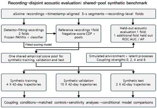
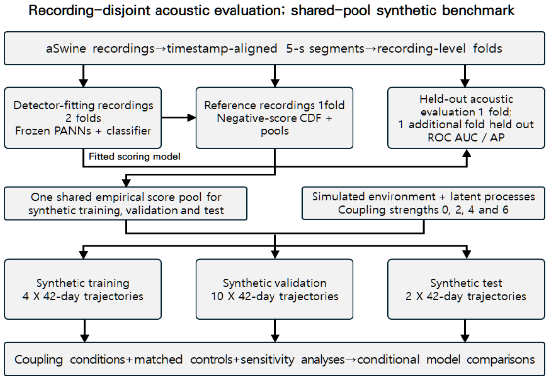
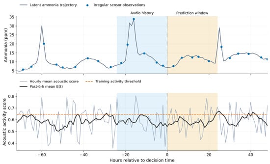
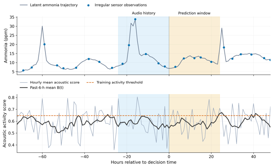
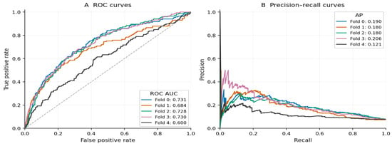
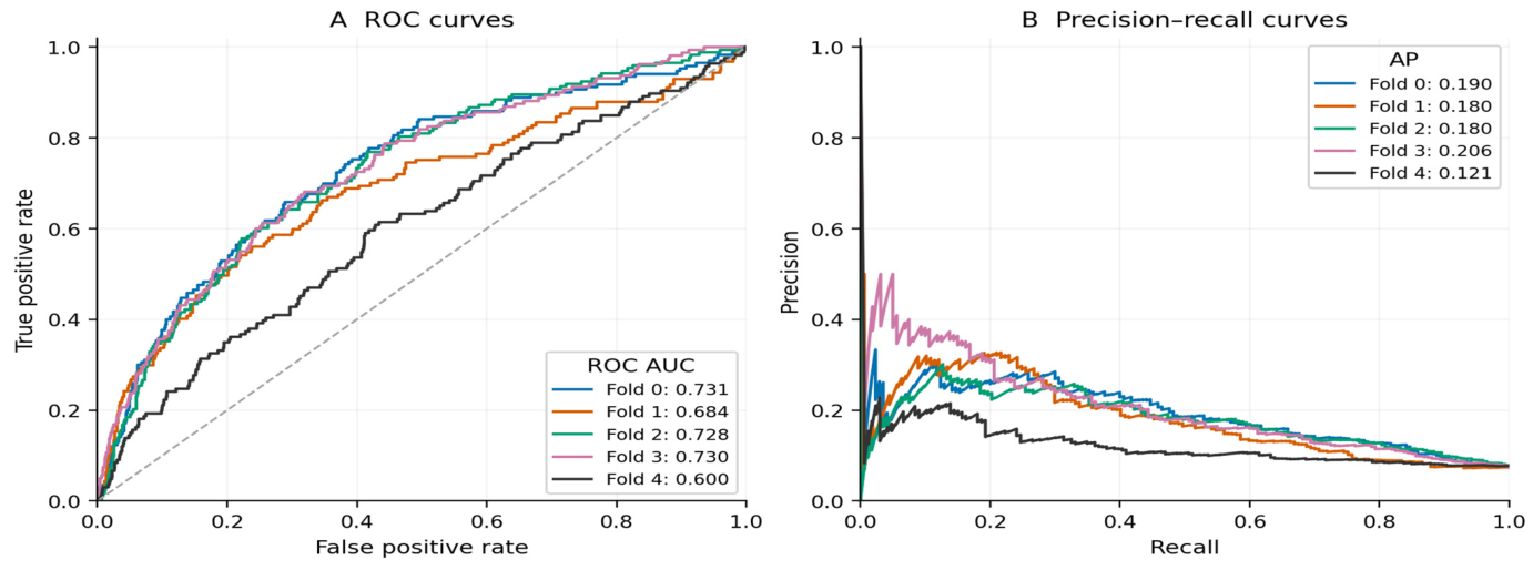
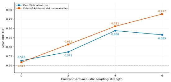
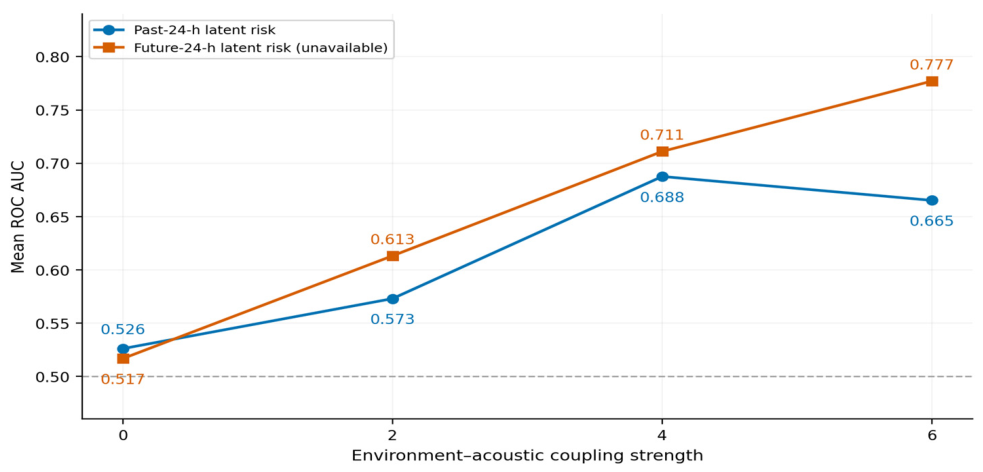
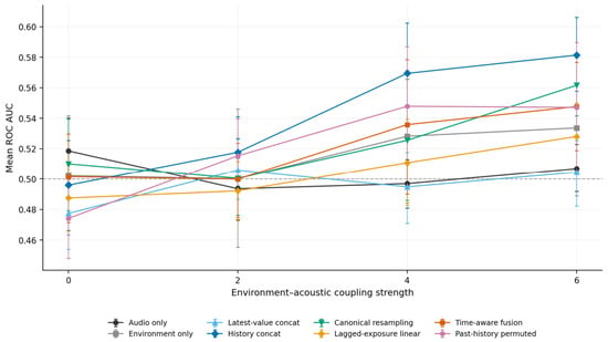
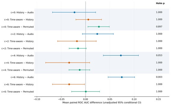
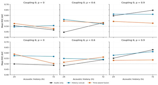
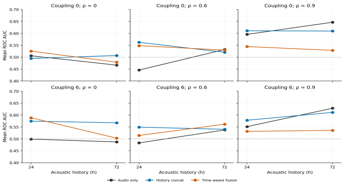
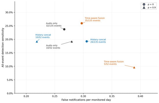
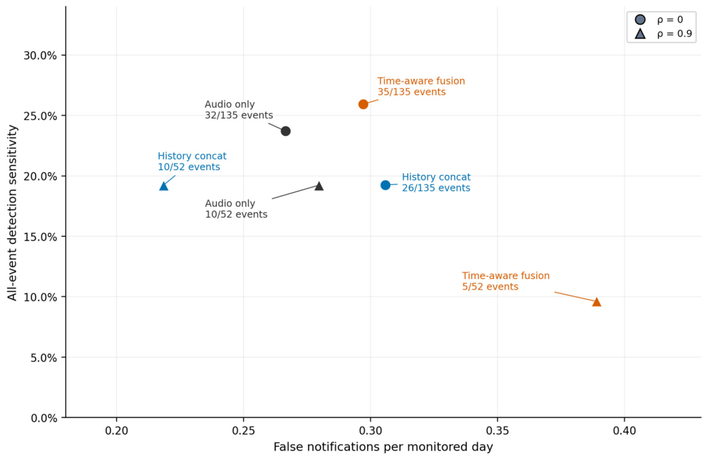

Disclaimer/Publisher’s Note: The statements, opinions and data contained in all publications are solely those of the individual author(s) and contributor(s) and not of MDPI and/or the editor(s). MDPI and/or the editor(s) disclaim responsibility for any injury to people or property resulting from any ideas, methods, instructions or products referred to in the content. |
© 2026 by the authors. Licensee MDPI, Basel, Switzerland. This article is an open access article distributed under the terms and conditions of the Creative Commons Attribution (CC BY) license.