Feasibility of Workstation-Level BLE Localization for Classroom Attendance: A Multi-Granularity Evaluation of Kalman-Filtered and Relational RSSI Features

Abstract

Credential-based attendance mechanisms such as QR codes and RFID cards record who checked in but not whether that person is physically present, which makes them vulnerable to proxy attendance. Vision-based alternatives depend on line of sight and camera coverage, whereas Bluetooth Low Energy (BLE) indoor positioning can passively verify the presence of a student’s device. However, received signal strength indicator (RSSI) measurements are highly sensitive to multipath propagation, so neighboring workstations with similar signal characteristics are difficult to distinguish. This study evaluates the feasibility of workstation-level BLE localization in a classroom with 40 workstations and four beacons. RSSI was smoothed with a Kalman filter and combined with relational features, namely beacon ranks and pairwise RSSI differences, as inputs to Weighted K-Nearest Neighbor (WKNN), Random Forest (RF), Extreme Gradient Boosting (XGBoost), and Support Vector Machine (SVM) classifiers at 40, 20, 8, and 4 location classes. Kalman filtering improved accuracy for all four models at every granularity (+3.34 to +11.89 percentage points); for the two main models, WKNN and RF, all paired cluster-bootstrap 95% confidence intervals of this gain were above zero (+4.58 to +8.71 percentage points). The relational features improved tree-based ensembles at 40 classes (RF: +1.38 percentage points, 95% CI [+0.03, +2.88]; XGBoost: +1.35 percentage points, point estimate) but reduced WKNN accuracy at the finer granularities. RF reached 40.68% accuracy at 40 classes, 61.06% at 8 classes, and 73.37% at 4 classes, and all four classifiers performed similarly at 40 classes. These results show a clear trade-off between spatial resolution and classification reliability with four beacons; identity binding and session-level attendance decisions remain to be evaluated.

1. Introduction

The attendance system plays a crucial role in monitoring human presence in the indoor environment. One implementation of an attendance system is in a classroom. Recording students’ presence in a classroom has been a strong indicator of academic success. A study from [1] shows that there is a strong relationship between students’ college grades and attendance. However, the traditional method of student absence recording requires a lot of time [2]. The traditional method of marking students’ absences requires forcing the teacher to call out students’ names one by one. This problem escalates with the number of students in a classroom. Recent studies have already developed smart attendance systems. Several studies employed computer vision to recognize students’ faces. The study by [3] proposed MobileNetV2 and a transfer learning method. Other pretrained models such as YoloV5 and VGGFace are used in the study by [4]. The CNN is also well known as being able to recognize someone’s face and has already been utilized in several studies [5,6]. However, computer vision with a face recognition approach is not always applicable in all conditions. Computer vision with single-camera solutions struggles in large classrooms with occlusion [7], poor lighting, limited viewpoints and the availability of the camera [8].

Beyond vision-based approaches, many institutions rely on credential-based attendance mechanisms such as QR-code scanning, Radio Frequency Identification (RFID) card tapping, or Learning Management System (LMS) check-ins. These mechanisms record who checked in but not whether that person is physically present in the classroom. A QR code can be forwarded through messaging applications or forged [9,10,11], and an RFID card can be tapped by another person [12], a practice commonly known as proxy attendance. This gap motivates an additional layer that verifies the physical presence of a student’s device in the classroom at check-in time. In this study, BLE-based indoor positioning is therefore considered not as a replacement for existing attendance mechanisms but as an auxiliary co-presence verification tier operating alongside them.

To realize such a passive verification layer, BLE-based indoor positioning systems have been studied. This approach requires Bluetooth beacons and users’ phones to get a Received Signal Strength Indicator (RSSI) value. An RSSI value is the most important data that enables indoor positioning systems. Based on [13], XGBoost shows exceptional performance among other models. Another study discovered that indoor localization can also be done using a Nearest Neighbor algorithm [14]. The feasibility of this approach has already been studied by [15], who utilize this technique as an intelligent approach for office rooms. These studies address indoor positioning as a discrete classification problem for predicting a specific location rather than continuous spatial coordinates. This classification performance heavily relies on RSSI fingerprinting, in which the distinct RSSI pattern associated with a given location serves as a reference for an unseen observation.

In this study, fine-grained localization refers to the ability to distinguish individual workstations within a dense classroom environment rather than merely identifying a broad room or zone. However, achieving such fine spatial resolution using BLE RSSI is challenging because neighboring workstations may exhibit highly similar signal characteristics due to multipath propagation and limited beacon density. Therefore, this study does not assume that individual-workstation localization can always be achieved with high accuracy. Instead, the proposed system evaluates multiple spatial granularities to investigate the practical resolution that can be supported by the deployed BLE infrastructure. Although room-level containment is the minimum requirement for co-presence verification, finer resolution would additionally enable seat-level consistency checks, for example, flagging multiple student accounts whose devices resolve to the same workstation.

Despite the promising results of indoor positioning systems using a Bluetooth approach, existing systems heavily rely on raw RSSI values. RSSI values are the most important data for estimating users’ positions, although their value is highly sensitive to surroundings. This is known as multipath propagation. Multipath propagation is a phenomenon where a wireless signal reaches its destination via multiple paths due to reflections, interference, walls and objects [16,17]. This drawback means that using the raw RSSI to estimate users’ positions is very unreliable. To enhance RSSI value integrity, studies use techniques such as filtering and temporal smoothing. One of the studies employed a Kalman filter (KF) to achieve a stable RSSI signal [18], and the KF has been widely applied to smooth RSSI measurements. Another approach is to use median filtering to preprocess RSSI values [19].

Despite these techniques, the RSSI signal still remains unstable when used as a single source of information, as these techniques only fix the variability in signal noise rather than resolve the underlying ambiguity in the signal. To address this limitation, several studies reformulate the RSSI signal representation into another form. Ref. [20] transformed the RSSI signal into a higher-dimensional data representation, such as an image, using the Markov Transition Field, enabling spatial signals to be captured through image-based feature extraction. Another strategy introduced in study [21] converts RSSI values into estimated distance to support geometry-based positioning through trilateration, rather than relying on the fingerprinting approach directly. These studies enabled the possibility of reformulating RSSI values into another representation beyond its raw scalar form, whether through alternative representations or derived features; this is a valid strategy to improve its reliability. Motivated by these studies, and by relational representations used in difference-based [22] and rank-based [23] fingerprinting, this study combines Kalman-filtered RSSI with beacon ranks and pairwise RSSI differences as inputs to learned classifiers. This approach also follows the principle of LANDMARC [24], which assumes that each location exhibits a distinct RSSI pattern relative to surrounding reference points, so that a location can be predicted through relative pattern matching rather than from a single absolute signal value. The main contributions of this study are:

1.

A relational fingerprint representation that combines Kalman-filtered RSSI with beacon ranks and pairwise RSSI differences as classifier inputs, which improves tree-based ensembles at workstation-level resolution (a marginally significant gain and a point-estimate gain for XGBoost), whereas it does not benefit distance-based WKNN.

2.

A feasibility evaluation of BLE RSSI-based localization in a 40-workstation classroom across four spatial granularities (40, 20, 8, and 4 classes), quantifying the trade-off between spatial resolution and classification reliability with four beacons.

With this approach, this study aims to evaluate whether temporal smoothing and a relational RSSI representation in the fingerprint improve the reliability of discrete location classification for a Bluetooth-based attendance system, and how this effect depends on the classifier and the spatial granularity. To evaluate the performance of the proposed method, several classification metrics were compared, such as accuracy, precision, recall and F1-score. This evaluation is expected to provide a comprehensive overview of the effectiveness of the proposed relational feature representation and temporal smoothing mechanism in discrete location classification. This study evaluates the localization layer of such a verification tier; identity binding, outside-room detection, and session-level attendance decisions are outside the experimental scope and are discussed in Section 4.

2. Materials and Methods

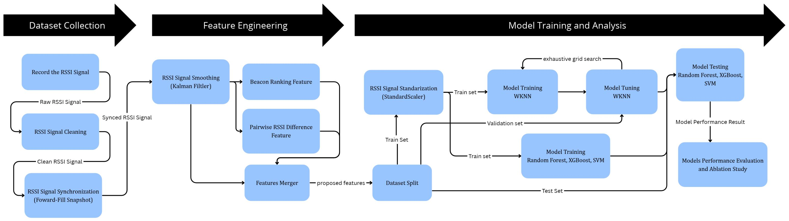
The steps of this study are shown in Figure 1. The process consists of several main steps: dataset collection, feature engineering, model training, ablation study and performance evaluation. The localization layer evaluated here is intended as an auxiliary, second-opinion co-presence check that operates alongside a primary credential-based attendance mechanism such as QR-code or RFID check-in; its output is therefore assessed as a location estimate rather than as a standalone attendance decision.

Figure 1. Proposed research methodology and experimental workflow.

2.1. Dataset Collection

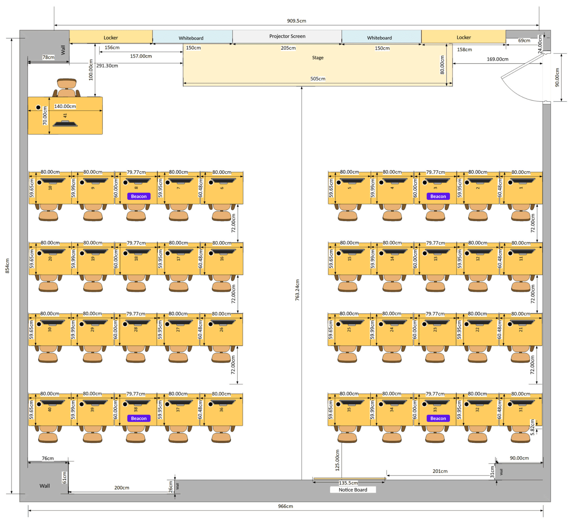
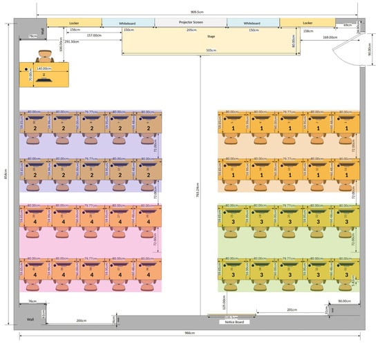
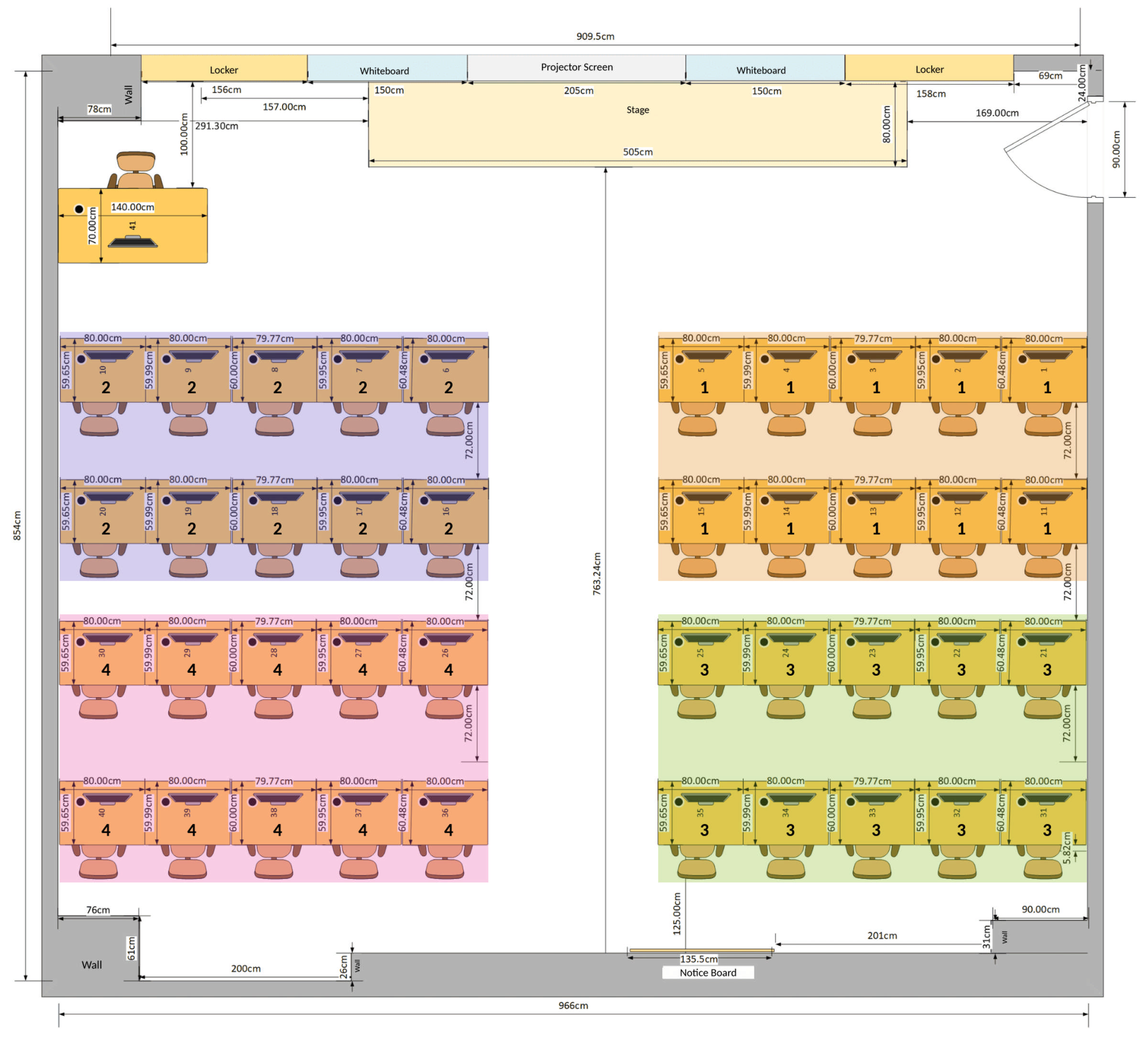
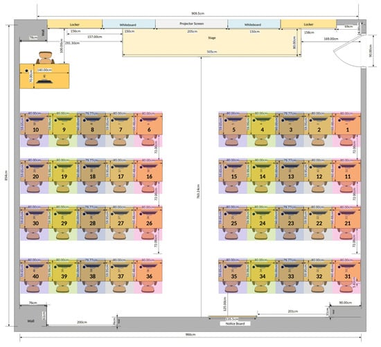
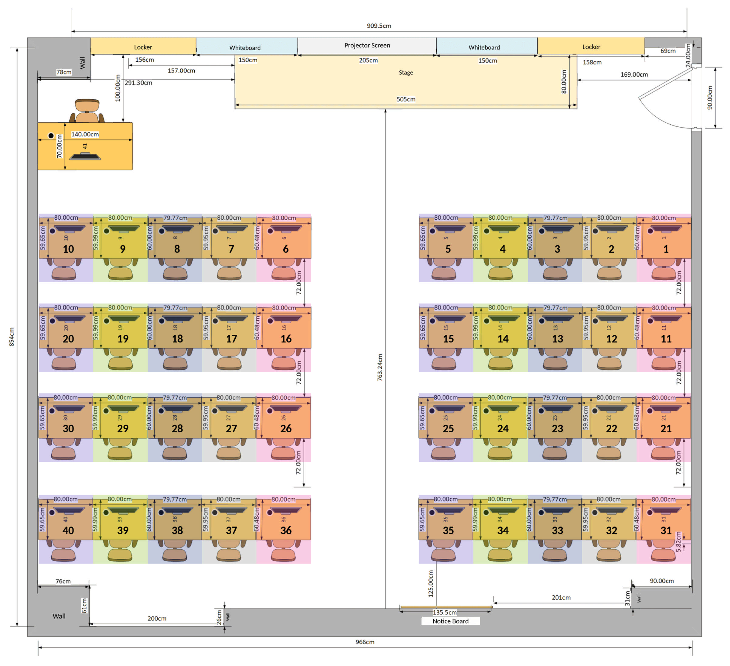
This study employed a self-collected dataset rather than using a publicly available dataset since there is no dataset available to match the specific beacon layout and deployment context targeted by this research. Data were collected in a classroom-sized room measuring 9.1 m × 8.5 m, containing 40 student workstations arranged in two blocks, each consisting of four rows with five workstations per row. Four Bluetooth Low Energy (BLE) beacons (UGREEN Bluetooth 6.0) were mounted above the middle workstation (the third of five workstations) in each of the four corner rows of the seating layout, i.e., the first and last row of each block. The detailed information about classroom layout and beacon position is illustrated in Figure 2.

Figure 2. Classroom layout used in this study (all dimensions in cm). Numbers 1–40 denote the student workstations and 41 the instructor’s desk; the purple labels mark the positions of the four beacons. This is the official floor plan of the room and is shown only to illustrate the spatial setup; the dimensions are not part of the experimental results.

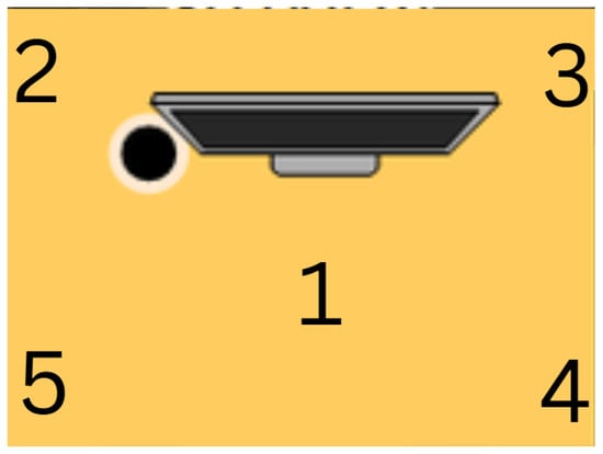
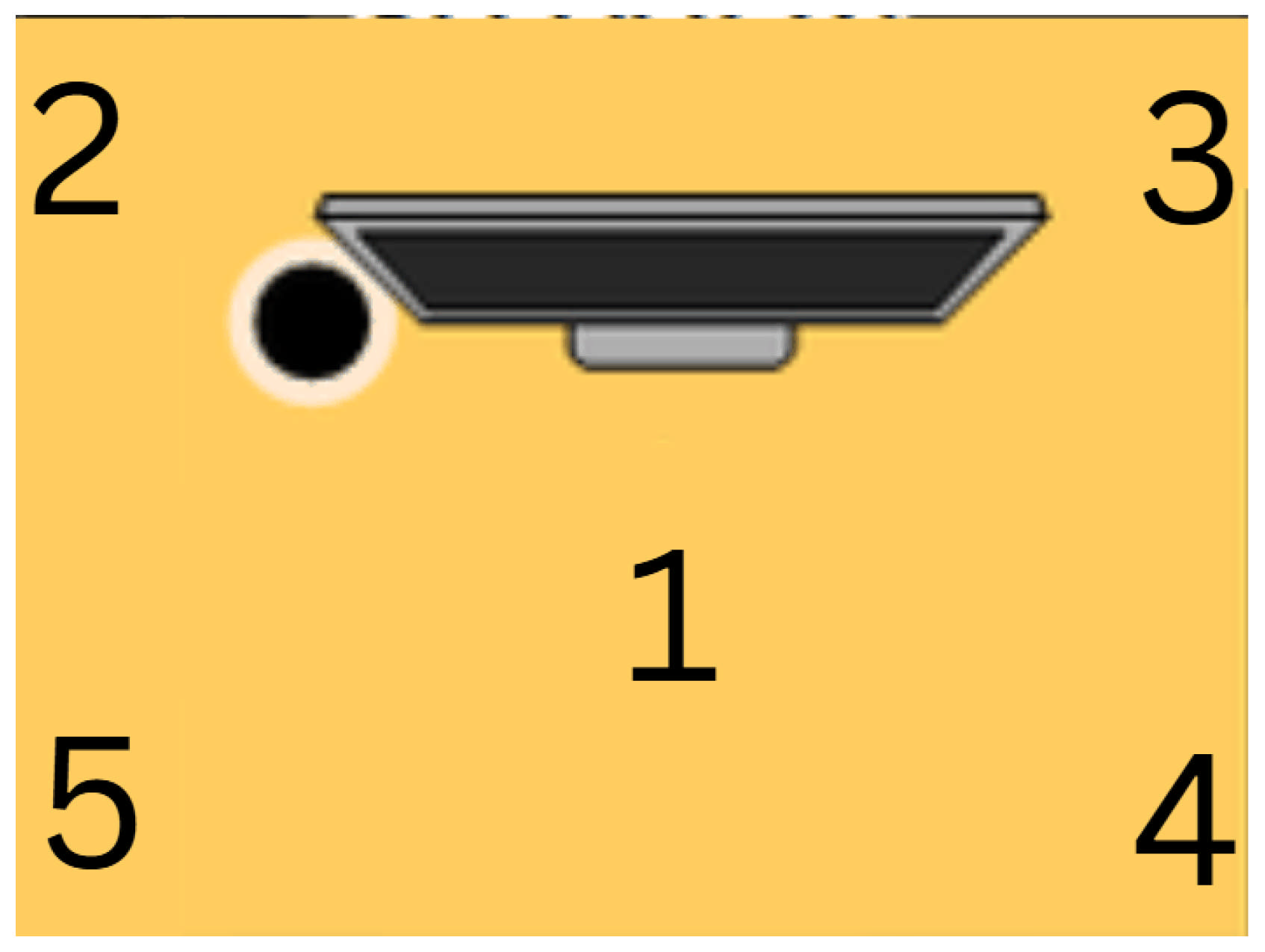
For each workstation, RSSI values were captured at five positions: one at the center and four at the corners of the workstation, yielding 200 distinct capture points. The capture position (Side) was recorded only as survey metadata and is not used as a model input. Data were collected using an iPhone 15 and the nRF Connect application, which scanned and logged the BLE advertisements of the beacons. During recording, the phone was held at the side of the surveyor’s body, on the north side, with an orientation deviation of approximately 0–20 degrees. Each capture point was recorded for approximately 90 s. The capture positions are illustrated in Figure 3.

Figure 3. Five RSSI recording positions at each individual workstation: (1) center, (2) top-left corner, (3) top-right corner, (4) bottom-right corner, and (5) bottom-left corner, as seen in the top view with the monitor at the top.

The raw log contained 37,026 entries, each corresponding to a single reading of one beacon. Two categories of entries were removed: 600 non-RSSI records (advertising interval metadata) and 39 entries with missing or invalid RSSI values, leaving 36,387 valid single-beacon readings, with RSSI values ranging from −100 to −36 dBm.

Because the receiver scans the beacons sequentially rather than simultaneously, each valid reading contains the RSSI of only one beacon, whereas the classifiers require one complete four-beacon vector per observation. An initial approach using fixed 1 s time bins was evaluated but discarded, as most bins contained incomplete beacon readings. Instead, a forward-fill snapshot approach with a staleness cutoff was used. Within each capture point, readings were indexed by their timestamps, and every timestamp at which at least one beacon was observed formed one snapshot; readings from several beacons sharing the same timestamp were merged into a single snapshot, which combined 8671 readings into 4256 snapshots and reduced the row count by 4415. Beacons not observed at a given timestamp were assigned their most recently observed value. To avoid pairing an outdated value with a fresh one, each forward-filled value was assigned an age, defined as the elapsed time since that beacon was last directly observed, and values older than 3 s, as well as beacons not yet observed at the start of a recording, were set to a placeholder of −100 dBm, corresponding to the weakest RSSI value observed in the log. The resulting dataset contains 31,972 synchronized snapshots, each with four RSSI values. The number of snapshots per workstation ranges from 382 to 949 (median 817, mean 799.3). Table 1 summarizes the record counts at each stage.

Table 1. Record counts at each data processing stage.

Stage	Operation	Records
Raw log	Single-beacon entries	37,026
Cleaning	Remove advertising interval records ($-600$) and invalid RSSI ($-39$)	36,387
Snapshot construction	Merge readings sharing a timestamp ($-4415$), forward-fill, staleness cutoff	31,972
Partitioning	Chronological split within each capture point	25,657 train/6315 test

2.2. Feature Engineering

The synchronized snapshots were then processed to obtain the filtered RSSI values and the relational features used in this study. Within each capture point, snapshots were ordered by their timestamps to obtain the chronological sequence required by the Kalman filter (KF).

The RSSI values of each snapshot were smoothed using a one-dimensional KF, applied independently to each beacon within each capture point. A random-walk state model was used, assuming that the underlying RSSI varies gradually over time and that each value is a noisy observation of it. The filter is defined as

$$({\widehat{x}}_t,P_t)=\left\{\begin{array}{cc}(-100,1),\hfill & z_t\le -99\hfill \\ \left({\displaystyle {\widehat{x}}_t^{-}}+K_t\left(z_t-{\displaystyle {\widehat{x}}_t^{-}}\right),(1-K_t){\displaystyle P_t^{-}}\right),\hfill & z_t>-99\hfill \end{array}\right.$$

(1)

$${\displaystyle {\widehat{x}}_t^{-}}=\left\{\begin{array}{cc}{z}_t,\hfill & {\widehat{x}}_{t-1}\le -99\hfill \\ {\widehat{x}}_{t-1},\hfill & {\widehat{x}}_{t-1}>-99\hfill \end{array}\right.{\displaystyle P_t^{-}}=\left\{\begin{array}{cc}1,\hfill & {\widehat{x}}_{t-1}\le -99\hfill \\ P_{t-1}+Q,\hfill & {\widehat{x}}_{t-1}>-99\hfill \end{array}\right.K_t={\displaystyle \frac{{\displaystyle P_t^{-}}}{{\displaystyle P_t^{-}}+R}}$$

(2)

where $z_t$ is the RSSI observation at time step t, ${\displaystyle {\widehat{x}}_t^{-}}$ and ${\displaystyle P_t^{-}}$ are the predicted (a priori) estimate and its error variance, ${\widehat{x}}_t$ is the filtered (a posteriori) estimate, $P_t$ is the estimation error variance, $K_t$ is the Kalman gain, Q is the process noise variance, and R is the measurement noise variance. The filter is initialized with ${\widehat{x}}_0=-100$ and $P_0=1$. The values $Q=0.05$ and $R=4.0$ were chosen empirically by visually inspecting the trade-off between noise suppression and responsiveness to genuine signal changes. When a beacon is not detected ($z_t\le -99$ dBm), its estimate is reset to the placeholder value with unit variance instead of being updated, so that a missing reading does not contaminate an otherwise valid trend. When readings resume after such a gap (${\widehat{x}}_{t-1}\le -99$), the filter is re-initialized from the new observation (${\displaystyle {\widehat{x}}_t^{-}}=z_t$, ${\displaystyle P_t^{-}}=1$). Because the filter is causal, each ${\widehat{x}}_t$ depends only on observations up to time t. All relational features below were derived from the filtered values, not from the raw readings.

Two relational feature groups were derived from the filtered RSSI values. Let ${\widehat{x}}_i$ denote the filtered RSSI of beacon i at a given time step (the time index t is omitted for brevity), and let $\widehat{\mathbf{x}}=({\widehat{x}}_1,{\widehat{x}}_2,{\widehat{x}}_3,{\widehat{x}}_4)$, where the indices correspond to the beacons at workstations 3, 8, 33, and 38, hereafter referred to as Beacons 1–4. Accordingly, ${\mathrm{RSSI}}_{\mathrm{Beacon}i}$ in the feature table denotes the Kalman-filtered value ${\widehat{x}}_i$. The pairwise difference features are defined as

$$D_{ij}={\widehat{x}}_i-{\widehat{x}}_j,1\le i<j\le 4,$$

(3)

yielding six features. The rank feature assigns each beacon its position when the four filtered values are sorted from strongest to weakest,

$$r_i=1+\sum _{j\ne i}⊮\left({\widehat{x}}_j>{\widehat{x}}_i\right),$$

(4)

where $⊮(·)$ is the indicator function, yielding four features, with ties assigned the same minimum rank (so that undetected beacons sharing $-100$ dBm receive an identical rank). Because $⊮({\widehat{x}}_j>{\widehat{x}}_i)=⊮(D_{ji}>0)$, the rank features encode the signs of the pairwise differences, whereas $D_{ij}$ retains their magnitudes. For example, for filtered values of $-60$, $-75$, $-50$, and $-80$ dBm at Beacons 1–4, the ranks are $(2,3,1,4)$ and $D_{12}=(-60)-(-75)=15$ dB, i.e., Beacon 1 is received 15 dB stronger than Beacon 2. The final input vector therefore contains 14 features: four filtered RSSI values, four ranks, and six pairwise differences.

Both feature groups are deterministic functions of $\widehat{\mathbf{x}}$ and thus add no information beyond it; their purpose is to change the representation presented to the classifier. The motivation follows the log-distance path-loss model, under which ${\widehat{x}}_i\approx A_i-10n{\log }_{10}{d}_i$, where $A_i$ is the reference power of beacon i, n the path-loss exponent, and $d_i$ the distance to beacon i. The difference $D_{ij}$ then depends on the distance ratio $d_i/d_j$ up to the constant offset $A_i-A_j$, so boundaries between neighboring workstations tend to be oblique in the RSSI feature space, and an offset common to all beacons, such as receiver gain, cancels [22]. Related representations have been used in difference-based [22] and rank-based [23] fingerprinting, where they replace absolute RSSI in distance-based matching; here, they are used alongside the filtered RSSI as inputs to learned classifiers.

2.3. Model Training and Analysis

The data were partitioned chronologically within each capture point rather than by random shuffling. For each of the 200 capture points, the first $\lceil 0.8N\rceil$ snapshots in recording order (approximately the first 72 s) formed the training segment and the remaining snapshots (approximately the last 18 s) formed the test segment, where N is the number of snapshots at that capture point. Because every capture point contributes to both partitions, all 40 workstation classes are represented in training and testing without a separate stratification step, and the partition is deterministic, so no random seed is involved. Since N varies between capture points (69–198 snapshots), the per-point rounding of this nominal 80:20 split yields 25,657 training and 6315 test samples overall (80.25% and 19.75%). For WKNN hyperparameter tuning, the training partition was further divided into fitting and validation subsets as described below, so that the data form three chronological sets: fitting, validation, and test.

Forward-filling and the Kalman filter were applied to each complete recording before partitioning; because both use only current and past readings, no information from a test segment enters the corresponding training segment. The forward-filled values and the filter state at the start of each test segment may carry over from the training segment. This protocol therefore evaluates short-term temporal reproducibility at known capture points.

All features were standardized to zero mean and unit variance using StandardScaler, which is required for distance- and kernel-based classifiers. The scaling parameters were estimated from training data only, i.e., from the fitting subset during hyperparameter tuning and from the complete training partition for the final models, and were then applied unchanged to the corresponding validation or test data, so that no test-set statistics enter the scaling. The fitted scaler was stored as a Joblib file so that the identical transformation could be applied to the test data and to future real-time predictions.

To examine the relationship between spatial resolution and classification performance, the original 40 workstation labels were organized into four spatial granularities of 4, 8, 20, and 40 classes, representing progressively finer location requirements. The 4-class configuration corresponds to coarse quadrant-level localization, the 8-class configuration to a finer zoning arrangement, the 20-class configuration to an intermediate resolution, and the 40-class configuration to individual-workstation localization. The grouping was defined according to the physical adjacency of workstations within each row and classroom block. By keeping the physical deployment fixed and varying only the label granularity, the experiment isolates the effect of spatial resolution on classification performance.

Four classifiers were evaluated: WKNN, RF, Extreme Gradient Boosting (XGBoost) [25], and a Support Vector Machine with a radial basis function kernel (SVM-RBF). WKNN and RF were selected as the main models, and XGBoost and SVM-RBF were added as benchmark classifiers representing gradient-boosted trees and kernel methods, the former having shown strong performance in related BLE localization work [13]. Deep learning models such as Convolutional Neural Networks (CNNs) were not used for three reasons. First, comparative studies on RSSI-based fingerprinting have demonstrated that RF achieves competitive performance relative to deep learning model [26,27]. Second, CNNs are architecturally designed to utilize spatial relationships between neighboring features, whereas RSSI fingerprint vectors are tabular in nature. Prior work has shown that applying CNNs to tabular data requires data transformation to an image-like representation [28,29]. Lastly, deep learning models require large training sets to generalize well; studies addressing limited-data fingerprinting scenarios have resorted to data augmentation or few-shot learning techniques to compensate for this requirement [30,31,32]. Given the self-collected dataset used in this study, conventional machine learning classifiers were considered more suitable.

All classifiers were trained independently and in parallel on the same training partition for each label granularity. WKNN assigns a query fingerprint $\mathbf{x}$ to the class with the largest weighted vote among its k nearest training samples ${\mathcal{N}}_k\left(\mathbf{x}\right)$:

$$\widehat{y}=\arg \underset{c}{\max }\sum _{i\in {\mathcal{N}}_k\left(\mathbf{x}\right)}{w}_i⊮(y_i=c),w_i={\displaystyle \frac{1}{d_p(\mathbf{x},{\mathbf{x}}_i)}},$$

(5)

where $d_p$ is the Minkowski distance of order p ($p=1$: Manhattan; $p=2$: Euclidean). If one or more neighbors lie at zero distance from the query ($d_p=0$), those neighbors receive unit weight and all other neighbors receive zero weight, so the prediction is determined by the exact matches. This case occurred for 4 of the 6315 test samples (0.06%).

The hyperparameters k and p were selected without using the test set. Within each capture point, the training segment was further split chronologically into a fitting subset (first 80%; 20,557 samples, 64.30% of all snapshots, approximately the first 58 s) and a validation subset (last 20%; 5100 samples, 15.95%, approximately the subsequent 14 s). The validation subset was used only for WKNN tuning; RF, XGBoost, and SVM-RBF, whose hyperparameters were fixed, were trained directly on the complete training partition. The StandardScaler and WKNN were fitted on the fitting subset, and a grid search over odd $k\in [1,201]$ and $p\in \{1,2\}$ was evaluated by validation accuracy. The selected configurations were $k=185$ for 4 classes, $k=107$ for 8 classes, $k=39$ for 20 classes, and $k=31$ for 40 classes, all with $p=2$. The scaler and model were then refit on the complete training partition (25,657 samples) and evaluated once on the held-out test set.

For RF, a fixed hyperparameter configuration was adopted and applied consistently across all four label granularities: 300 decision trees, a maximum tree depth of 30, a minimum of 5 samples required to split an internal node, a minimum of 4 samples per leaf, sqrt-based feature subsampling, balanced class weighting to mitigate the effect of label imbalance across workstations, and a fixed random seed of 42.

XGBoost used 300 estimators, a maximum depth of 6, a learning rate of 0.1, and row and column subsampling ratios of 0.8, and SVM-RBF used $C=10$ with $\gamma$ set to the scikit-learn default (scale). The RF, XGBoost, and SVM hyperparameters were fixed a priori and were not tuned on the test set. All trained models were evaluated on the held-out test set, and the results were used for model comparison and for the ablation study.

2.4. Ablation Study

An ablation study was conducted in this study to evaluate the individual and combined contribution of the proposed relational RSSI features and the effect of label granularity on classification performance. The ablation study was structured into two parts: feature contribution ablation and label granularity ablation.

2.4.1. Feature Contribution Ablation

To isolate the contribution of each proposed feature, five feature configurations were evaluated. Configuration A serves as the reference feature configuration, using the raw RSSI signal without filtering. Configuration B introduces KF, isolating the effect of signal smoothing. Configuration C and D each add one relational feature, beacon ranking and pairwise RSSI difference, on top of the KFed signal. Configuration E combines all proposed features, representing the complete feature set proposed in this study. The configurations are summarized in Table 2.

Table 2. Feature configurations used in the feature contribution ablation.

Config.	Description
A	Raw RSSI
B	KF only
C	KF + Beacon Ranking
D	KF + RSSI Difference
E	KF + Ranking + RSSI Difference (Proposed)

2.4.2. Label Granularity Ablation

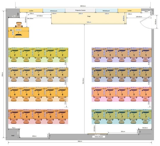
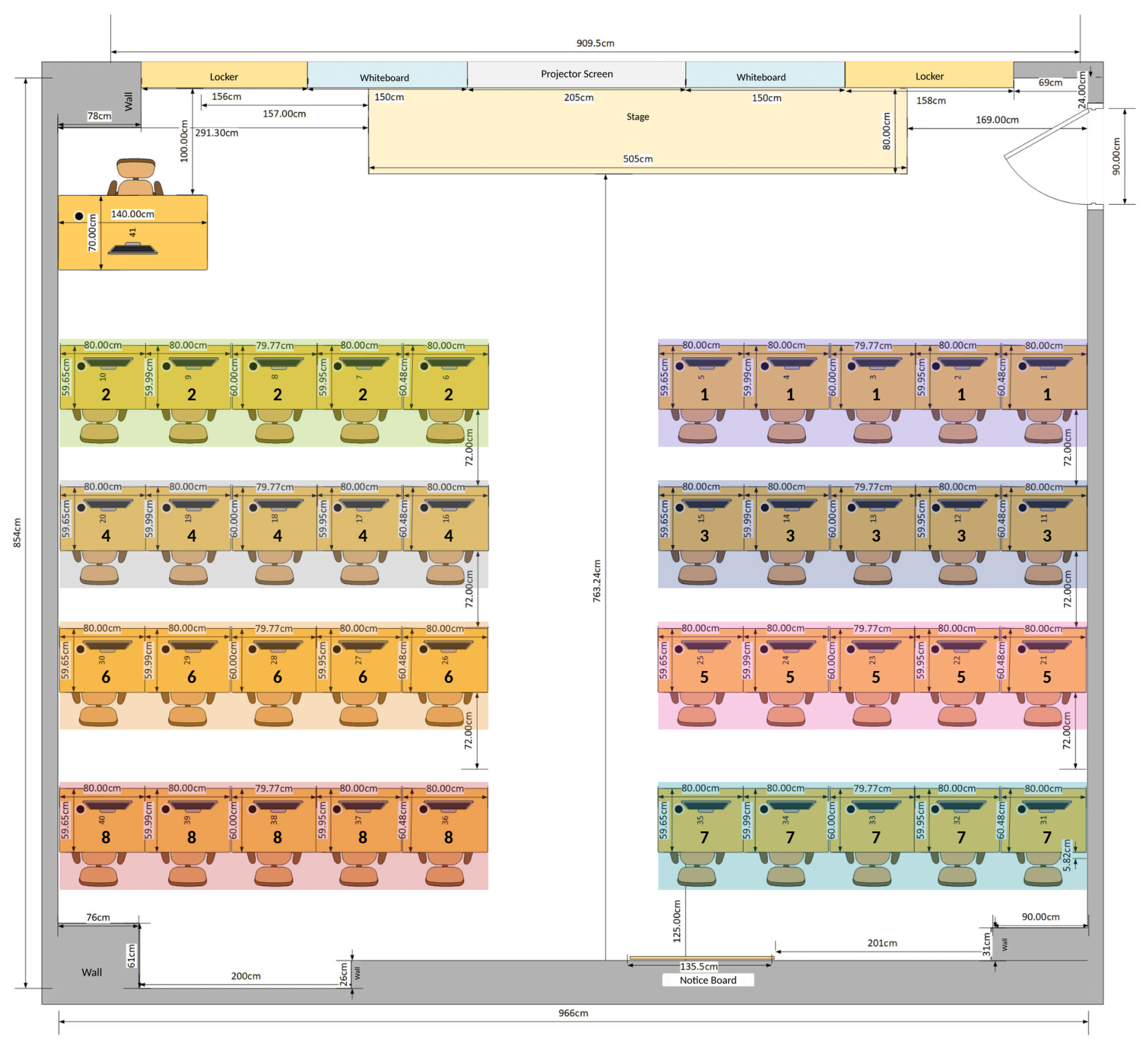
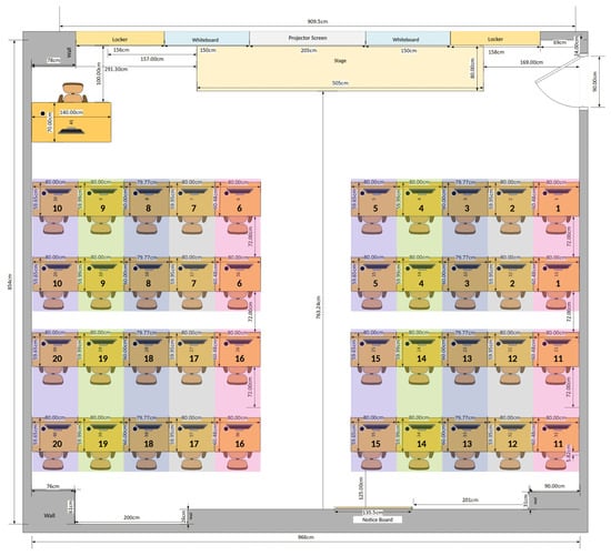
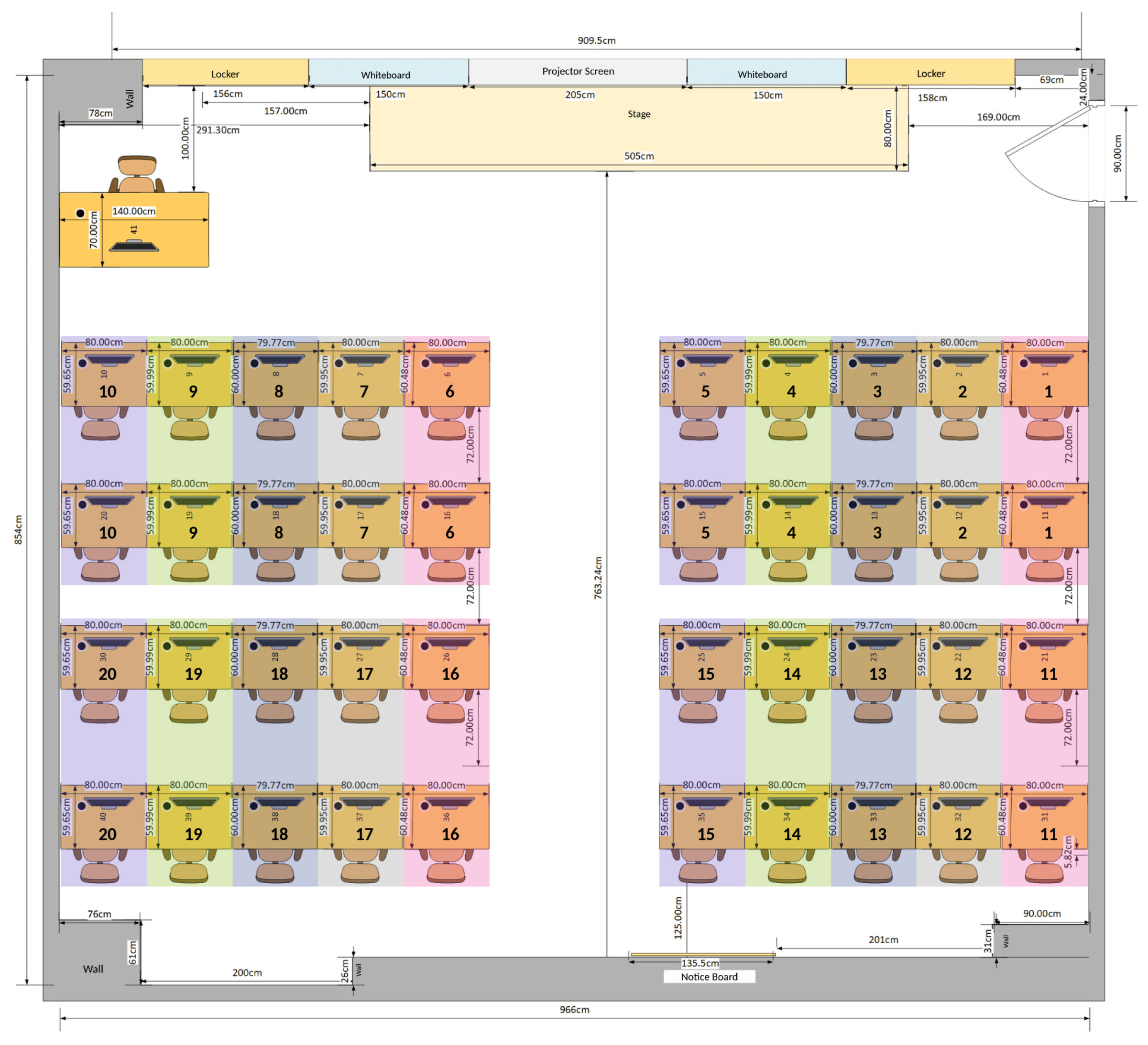
Using configuration E, the effect of label granularity on classification performance was subsequently evaluated. The original 40 class labels were grouped into 20, 8, and 4 coarser granularities based on physical adjacency within each row and block. The 40-label configuration serves as the baseline granularity against which the coarser granularities are compared. All models were retrained and evaluated at each of the four granularity levels using an identical train–test split, in order to assess the trade-off between spatial resolution and classification accuracy. The result of grouped labels are illustrated in Figure 4, Figure 5 and Figure 6. The original 40 labels is illustrated in Figure 7.

Figure 4. Grouping method for 4 labels. Each block of two rows of five workstations forms one class; the bold number on each workstation indicates its class label, and each color denotes one class. All dimensions are in cm.

Figure 5. Grouping method for 8 labels. Each row of five workstations forms one class; the bold number on each workstation indicates its class label, and each color denotes one class. All dimensions are in cm.

Figure 6. Grouping method for 20 labels. Each pair of vertically aligned workstations forms one class; the bold number on each workstation indicates its class label, and each color denotes one class. All dimensions are in cm.

Figure 7. Label assignment for the 40-label configuration. Each workstation forms its own class, and the large bold number indicates its class label (identical to the workstation number in this configuration). Colors are used only to visually distinguish adjacent workstations. All dimensions are in cm.

2.4.3. Statistical Comparison of Configurations

Because consecutive snapshots within a capture point are temporally correlated, the test samples are not independent, and resampling individual snapshots would underestimate the uncertainty. Differences between configurations were therefore assessed with a paired cluster bootstrap in which the 200 capture points serve as the resampling units. In each of $B=1000$ iterations, 200 capture points were drawn with replacement, all test snapshots of the drawn capture points were pooled, and the accuracy of both compared configurations was computed on this same resampled set. The 95% confidence interval of the paired accuracy difference was obtained from the 2.5th and 97.5th percentiles of the 1000 differences. This procedure was applied to the effect of Kalman filtering (B − A) and of the relational features (E − B) for the two main models, WKNN and RF, at each granularity. For the benchmark classifiers (XGBoost and SVM-RBF), only the sample-level point differences are reported.

2.5. Model Performance Evaluation

Model performance was evaluated using accuracy, macro-averaged precision, macro-averaged recall, and macro-averaged F1-score, complemented by confusion-matrix and localization-error analyses for the main models. Accuracy measures the overall proportion of correctly classified samples:

$$\mathrm{Accuracy}={\displaystyle \frac{{\displaystyle {\sum }_{i=1}^C}{\mathrm{TP}}_i}{N}},$$

(6)

where ${\mathrm{TP}}_i$ is the number of correctly classified samples of class i, C is the number of location classes, and N is the total number of test samples.

Accuracy served as the main basis for comparison across models and the four label granularities. In addition, precision, recall, and F1-score were computed for each model at each granularity. Precision measures the proportion of predictions for a class that are correct, whereas recall measures the proportion of actual samples of a class that are correctly identified:

$${\mathrm{Precision}}_i={\displaystyle \frac{{\mathrm{TP}}_i}{{\mathrm{TP}}_i+{\mathrm{FP}}_i}},{\mathrm{Recall}}_i={\displaystyle \frac{{\mathrm{TP}}_i}{{\mathrm{TP}}_i+{\mathrm{FN}}_i}},$$

(7)

where ${\mathrm{FP}}_i$ is the number of samples of other classes incorrectly predicted as class i, and ${\mathrm{FN}}_i$ is the number of samples of class i incorrectly predicted as another class. The F1-score combines precision and recall into a single value:

$${\mathrm{F}1}_i=2·{\displaystyle \frac{{\mathrm{Precision}}_i·{\mathrm{Recall}}_i}{{\mathrm{Precision}}_i+{\mathrm{Recall}}_i}}.$$

(8)

The per-class values were macro-averaged, i.e., computed as the unweighted mean over the C classes (e.g., $\mathrm{Macro}-\mathrm{F}1={\displaystyle \frac{1}{C}}{\displaystyle {\sum }_{i=1}^C}{\mathrm{F}1}_i$), so that every location class contributes equally regardless of its number of samples. These macro-averaged metrics therefore reveal whether performance is consistent across all locations rather than being dominated by frequently occurring classes.

Because the classification metrics treat every incorrect prediction equally, regardless of how far the predicted location is from the true one, two complementary analyses were performed for the main models (WKNN and RF). First, confusion matrices were inspected to determine whether misclassifications occur between physically adjacent classes or are scattered across the room. Second, a localization error was computed for each test snapshot as the Euclidean distance (in meters) between the reference coordinates of the true and the predicted class, where the reference coordinate is the center of the workstation for the 40-class configuration and the centroid of the grouped workstations for the coarser configurations; a correct prediction therefore has an error of 0 m. The cumulative distribution function (CDF) of this error is reported together with its median and 80th percentile.

3. Results

The experimental results are presented in this section, following the methodology outlined in Figure 1.

3.1. Dataset Collection and RSSI Signal Cleaning

The raw log collected during the experimental campaign contains a total of 37,026 entries, from which 36,387 valid single-beacon RSSI readings were obtained after removing advertising interval metadata and missing values. The measured RSSI values range from $-100.0\mathrm{dBm}$ to $-36.0\mathrm{dBm}$, representing the variation in received signal strength under the tested recording conditions. These readings were subsequently synchronized and consolidated into 31,972 complete four-beacon snapshots for model training and evaluation (as detailed in Table 1). A summary of the raw recording characteristics is presented in Table 3.

Table 3. Evaluation raw RSSI Dataset.

Description	Value
Total Dataset Recorded	37,026 lines
Min RSSI	$-100.0$ dBm
Max RSSI	$-36.0$ dBm
Position of Side-Body Recording	North side with an angular deviation of 0–20 degrees

3.2. Feature Extraction and Dataset Representation

Subsequent feature extraction was performed as proposed in Figure 1. Feature engineering was conducted utilizing the KF, Beacon Ranking, and Pairwise RSSI Difference features, which were subsequently concatenated into a single large dataset for subsequent processing. This resulted in the dataset structure shown in Table 4.

Table 4. Dataset variables and distinction between metadata and model input predictors. Beacons 1–4 correspond to beacons 3, 8, 33, and 38.

Variable Name	Description & Role in Classification
A. Metadata & Ground Truth (Strictly Excluded from Model Inputs)
Table	Ground truth target class (Workstations 1–40, mapped into 40, 20, 8, or 4 categories).
Side	Capture position at the workstation (1–5: one center and four corners; see Figure 3). Note: Excluded from model predictors; not required at deployment.
Sample	Timestamp sequence index within 90-s recording burst (Excluded from predictors).
B. Actual Model Input Predictors (14 Features Fed to Classifiers)
RSSI KF Beacon 1	1D Kalman-filtered smoothed RSSI of Beacon 3
RSSI KF Beacon 2	1D Kalman-filtered smoothed RSSI of Beacon 8
RSSI KF Beacon 3	1D Kalman-filtered smoothed RSSI of Beacon 33
RSSI KF Beacon 4	1D Kalman-filtered smoothed RSSI of Beacon 38
Rank Beacon 1	Ordinal signal strength rank (1–4) of Beacon 3
Rank Beacon 2	Ordinal signal strength rank (1–4) of Beacon 8
Rank Beacon 3	Ordinal signal strength rank (1–4) of Beacon 33
Rank Beacon 4	Ordinal signal strength rank (1–4) of Beacon 38
Diff Beacon 1 2	Pairwise RSSI difference (${\mathrm{RSSI}}_{\mathrm{Beacon}1}-{\mathrm{RSSI}}_{\mathrm{Beacon}2}$)
Diff Beacon 1 3	Pairwise RSSI difference (${\mathrm{RSSI}}_{\mathrm{Beacon}1}-{\mathrm{RSSI}}_{\mathrm{Beacon}3}$)
Diff Beacon 1 4	Pairwise RSSI difference (${\mathrm{RSSI}}_{\mathrm{Beacon}1}-{\mathrm{RSSI}}_{\mathrm{Beacon}4}$)
Diff Beacon 2 3	Pairwise RSSI difference (${\mathrm{RSSI}}_{\mathrm{Beacon}2}-{\mathrm{RSSI}}_{\mathrm{Beacon}3}$)
Diff Beacon 2 4	Pairwise RSSI difference (${\mathrm{RSSI}}_{\mathrm{Beacon}2}-{\mathrm{RSSI}}_{\mathrm{Beacon}4}$)
Diff Beacon 3 4	Pairwise RSSI difference (${\mathrm{RSSI}}_{\mathrm{Beacon}3}-{\mathrm{RSSI}}_{\mathrm{Beacon}4}$)

3.3. Dataset Split and RSSI Signal Standarization

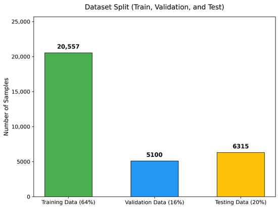
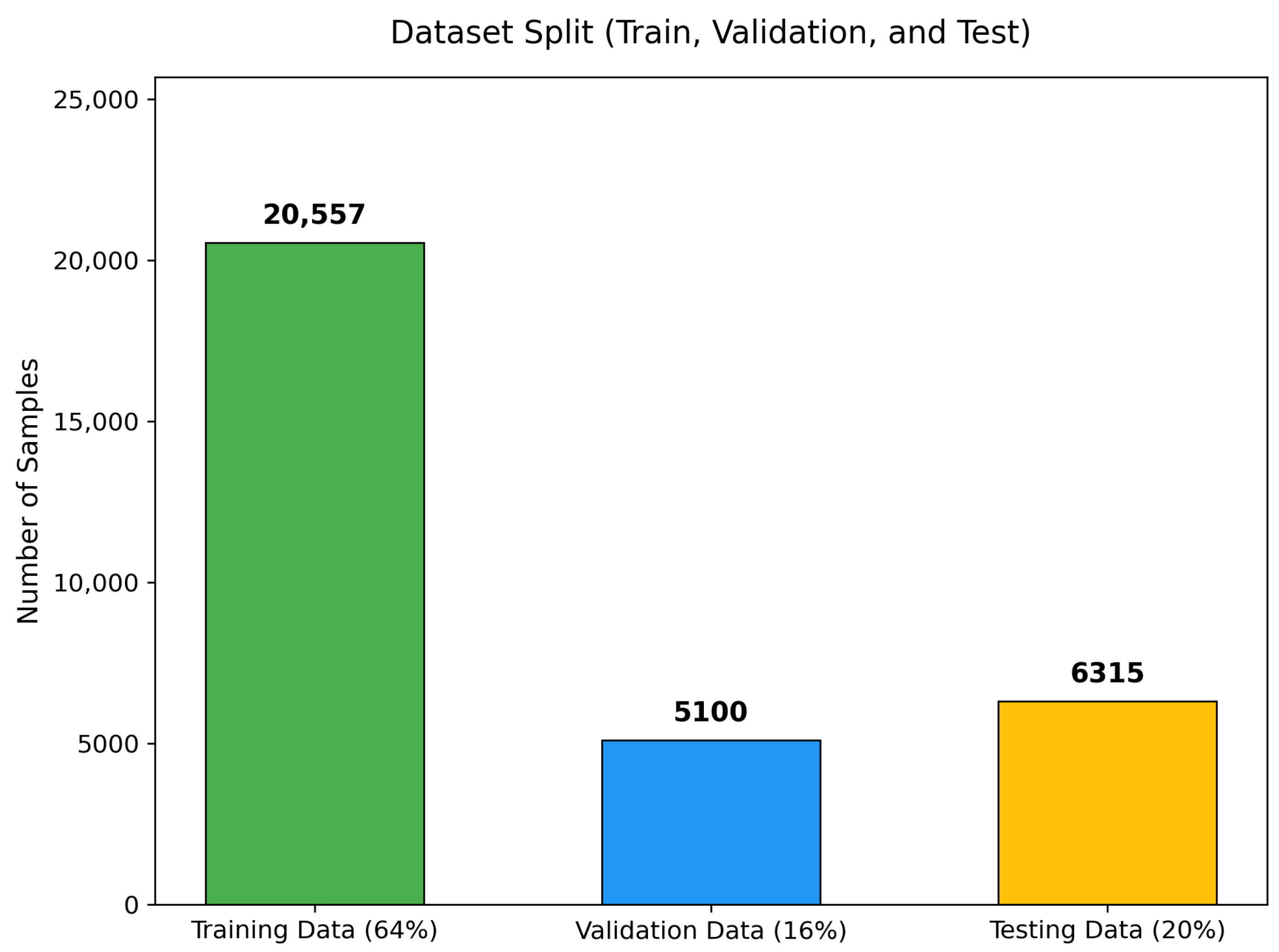
To strictly prevent temporal data leakage, data partitioning was conducted deterministically on a chronological basis within each of the 200 physical capture points ($\mathrm{Table}\times \mathrm{Side}$). An 80:20 chronological ratio was applied locally to each point’s continuous recording. Because the number of received snapshots per point varied discretely (between 69 and 198 samples due to asynchronous BLE advertising reception), local integer boundary rounding resulted in cumulative totals of 25,657 samples (80.25%) for model development (the initial ∼72 s) and 6315 samples (19.75%) reserved as a strictly held-out testing set (the final ∼18 s), totaling 31,972 samples (as illustrated in Figure 8). Furthermore, to prevent data snooping during hyperparameter tuning, the development set was hierarchically partitioned using the same chronological rule into an inner-fitting subset of 20,557 samples (64.30% of total data, representing the first ∼58 s) and an inner-validation subset of 5100 samples (15.95% of total data, representing the subsequent ∼14 s). The inner-validation set was utilized exclusively to optimize model hyperparameters (such as grid-searching the neighbor parameter k and distance metric for WKNN), while the held-out testing set remained completely untouched until final benchmark evaluation. This chronological three-way separation guarantees that neither model parameters nor hyperparameter selection are influenced by temporally subsequent observations or final testing samples.

Figure 8. Chronological dataset partitioning across the training, validation, and testing subsets.

3.4. Model Training and Hyperparameter Tuning

Parallel model training was executed following the architecture shown in Figure 1. To ensure numerical stability, a standard scaler is fitted to the training set to normalize the data. The fitted scaler object is then saved as a Joblib file, allowing it to be loaded for transforming the testing data and future real-time predictions without causing data leakage.

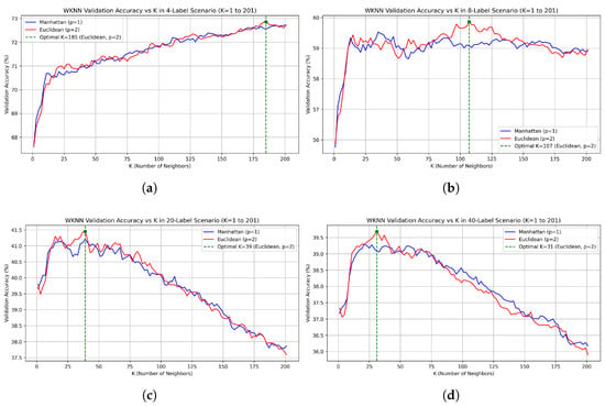
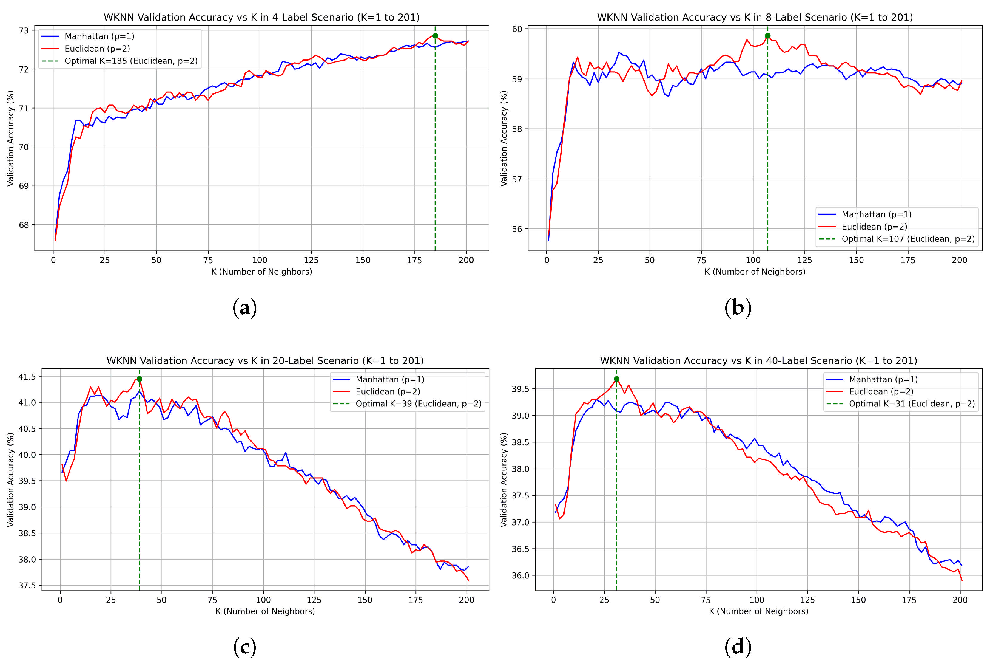
This hyperparameter search was repeated independently across the four spatial granularities shown in Figure 7 through Figure 4. The resulting validation accuracy curves across odd $k\in [1,201]$ and $p\in \{1,2\}$ are presented in Figure 9.

Figure 9. Validation accuracy comparison of the WKNN algorithm across odd hyperparameter k (ranging from 1 to 201) evaluated strictly on the inner-validation subset (5100 samples) using Euclidean ($p=2$) and Manhattan ($p=1$) distance metrics: (a) 4-label scenario ($k=185,p=2$); (b) 8-label scenario ($k=107,p=2$); (c) 20-label scenario ($k=39,p=2$); and (d) 40-label scenario ($k=31,p=2$). The green marker and dashed vertical line in each plot indicate the optimal configuration selected for the final refitted model.

Based on the inner-validation tuning profiles illustrated in Figure 9, the optimal neighborhood size systematically decreases as the spatial zoning granularity becomes finer, while Euclidean distance ($p=2$) consistently outperforms Manhattan distance ($p=1$) across all four scenarios. Specifically, the 4-label quadrant scenario achieved its highest validation accuracy (72.86%) at $k=185$ ($p=2$), whereas the 8-label row-level scenario peaked (59.86%) at $k=107$ ($p=2$). For the finer-grained configurations, the required neighborhood size contracted further, with the 20-label and 40-label scenarios reaching optimal validation accuracies of 41.45% at $k=39$ ($p=2$) and 39.69% at $k=31$ ($p=2$), respectively. These validation-selected hyperparameters were then locked and used to refit the final WKNN models on the complete training partition (25,657 samples) for subsequent evaluation and ablation analysis.

3.5. Evaluation and Ablation Study

Following model training, classification performance was evaluated on the 20% temporally held-out test set (6315 samples) across all four spatial granularities: 40, 20, 8, and 4 labels. To provide a rigorous cross-paradigm benchmark, the primary WKNN and Random Forest models are compared against Extreme Gradient Boosting (XGBoost) and a Support Vector Machine with a radial basis function kernel (SVM-RBF). The complete benchmark results are summarized in Table 5, demonstrating a clear trade-off between spatial resolution and classification reliability.

Table 5. Evaluation Results of WKNN, Random Forest, XGBoost, and SVM-RBF Models.

Model	Scenario	Performance Metrics
		Accuracy	Precision	Recall	F1-Score
WKNN	40 Labels	38.94%	38.09%	38.37%	37.46%
	20 Labels	41.60%	40.49%	40.61%	40.14%
	8 Labels	60.62%	62.28%	60.45%	60.75%
	4 Labels	73.79%	73.63%	73.12%	72.84%
Random Forest	40 Labels	40.68%	40.22%	40.28%	39.73%
	20 Labels	43.82%	43.12%	42.98%	42.82%
	8 Labels	61.06%	61.96%	61.20%	61.34%
	4 Labels	73.37%	72.96%	72.88%	72.75%
XGBoost	40 Labels	39.67%	39.49%	39.08%	38.70%
	20 Labels	43.36%	42.46%	42.44%	42.22%
	8 Labels	60.59%	61.84%	60.50%	60.84%
	4 Labels	73.05%	72.60%	72.43%	72.32%
SVM-RBF	40 Labels	39.64%	39.88%	39.30%	38.16%
	20 Labels	42.50%	42.01%	41.46%	40.89%
	8 Labels	59.86%	61.23%	59.77%	59.80%
	4 Labels	74.65%	74.70%	74.02%	73.72%

In the 40-label scenario, representing individual workstation localization, all four classifiers encountered a similar performance ceiling due to severe signal overlap in the dense indoor environment. The Random Forest model achieved the highest accuracy at 40.68%, with precision at 40.22%, recall at 40.28%, and an F1-score of 39.73%. SVM-RBF and XGBoost followed closely with accuracies of 39.64% (precision: 39.88%, recall: 39.30%, F1-score: 38.16%) and 39.67% (precision: 39.49%, recall: 39.08%, F1-score: 38.70%), respectively, while the WKNN model yielded 38.94% accuracy, 38.09% precision, 38.37% recall, and a 37.46% F1-score. Notably, the tight convergence of four fundamentally distinct algorithmic families within a narrow range of 38.94–40.68% indicates that fine-grained accuracy is bounded by the physical propagation ceiling of the four-beacon setup rather than classifier capacity. Although mathematically modest, the confusion matrix analysis reveals a strong diagonal tendency. This indicates that misclassifications primarily occur in the immediate physical vicinity rather than randomly across the room, reflecting the difficulty of distinguishing highly overlapping Bluetooth signals among closely spaced tables.

When the spatial resolution was reduced to 20 labels, performance showed a marginal improvement of approximately 3–4%. Random Forest accuracy increased to 43.82% (precision: 43.12%, recall: 42.98%, F1: 42.82%), while XGBoost and SVM-RBF reached 43.36% (precision: 42.46%, recall: 42.44%, F1: 42.22%) and 42.50% (precision: 42.01%, recall: 41.46%, F1: 40.89%), respectively. Similarly, WKNN accuracy rose to 41.60% (precision: 40.49%, recall: 40.61%, F1: 40.14%). This minimal gain suggests that merely pairing two adjacent seats into one label is still insufficient to fully resolve the multipath propagation ambiguity caused by the limited beacon density.

A significant performance shift occurred in the 8-label scenario, where accuracy increased by roughly 20% compared with the baseline. Random Forest achieved 61.06% accuracy (precision: 61.96%, recall: 61.20%, F1: 61.34%), while WKNN followed closely with 60.62% accuracy (precision: 62.28%, recall: 60.45%, F1: 60.75%), alongside XGBoost at 60.59% (precision: 61.84%, recall: 60.50%, F1: 60.84%) and SVM-RBF at 59.86% (precision: 61.23%, recall: 59.77%, F1: 59.80%). By grouping workstations into broader physical zones, the RSSI fingerprints became far more distinct, effectively reducing classification ambiguity and signal interference.

Finally, in the 4-label scenario, representing the lowest classification complexity (quadrant-level localization), all four models reached their peak performance. The SVM-RBF model achieved the highest accuracy at 74.65% (precision: 74.70%, recall: 74.02%, F1: 73.72%), followed by the WKNN model at 73.79% accuracy (precision: 73.63%, recall: 73.12%, F1: 72.84%), Random Forest at 73.37% accuracy (precision: 72.96%, recall: 72.88%, F1: 72.75%), and XGBoost at 73.05% accuracy (precision: 72.60%, recall: 72.43%, F1: 72.32%).

These progressive results confirm that while pinpointing an individual seat (40 labels) using BLE RSSI is challenging without denser beacon infrastructure, adopting a zone-based attendance approach (8 or 4 labels) provides a highly robust and reliable localization alternative across all evaluated classifier families.

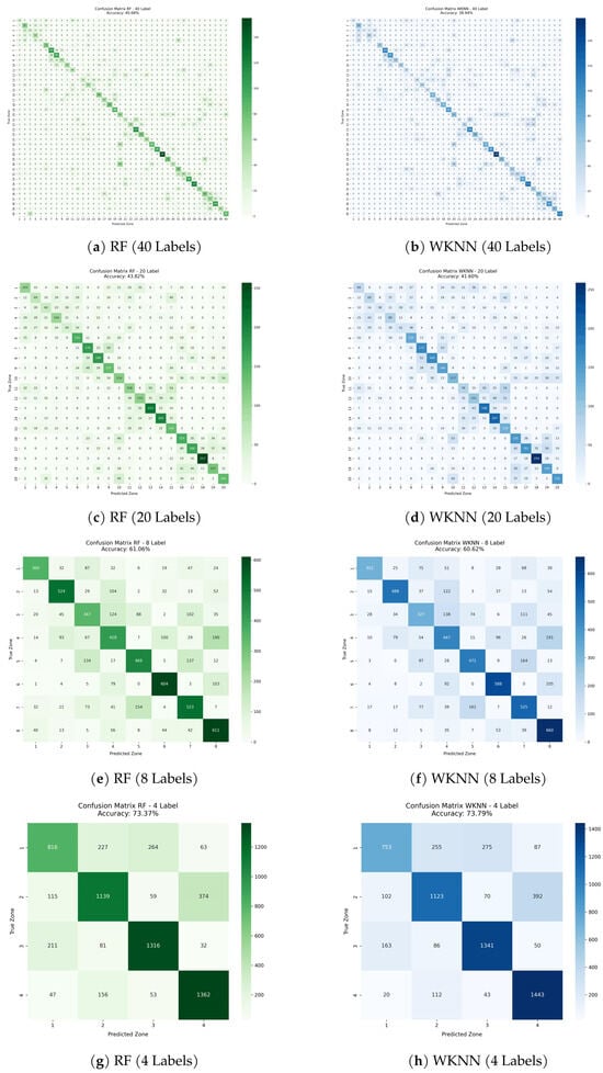
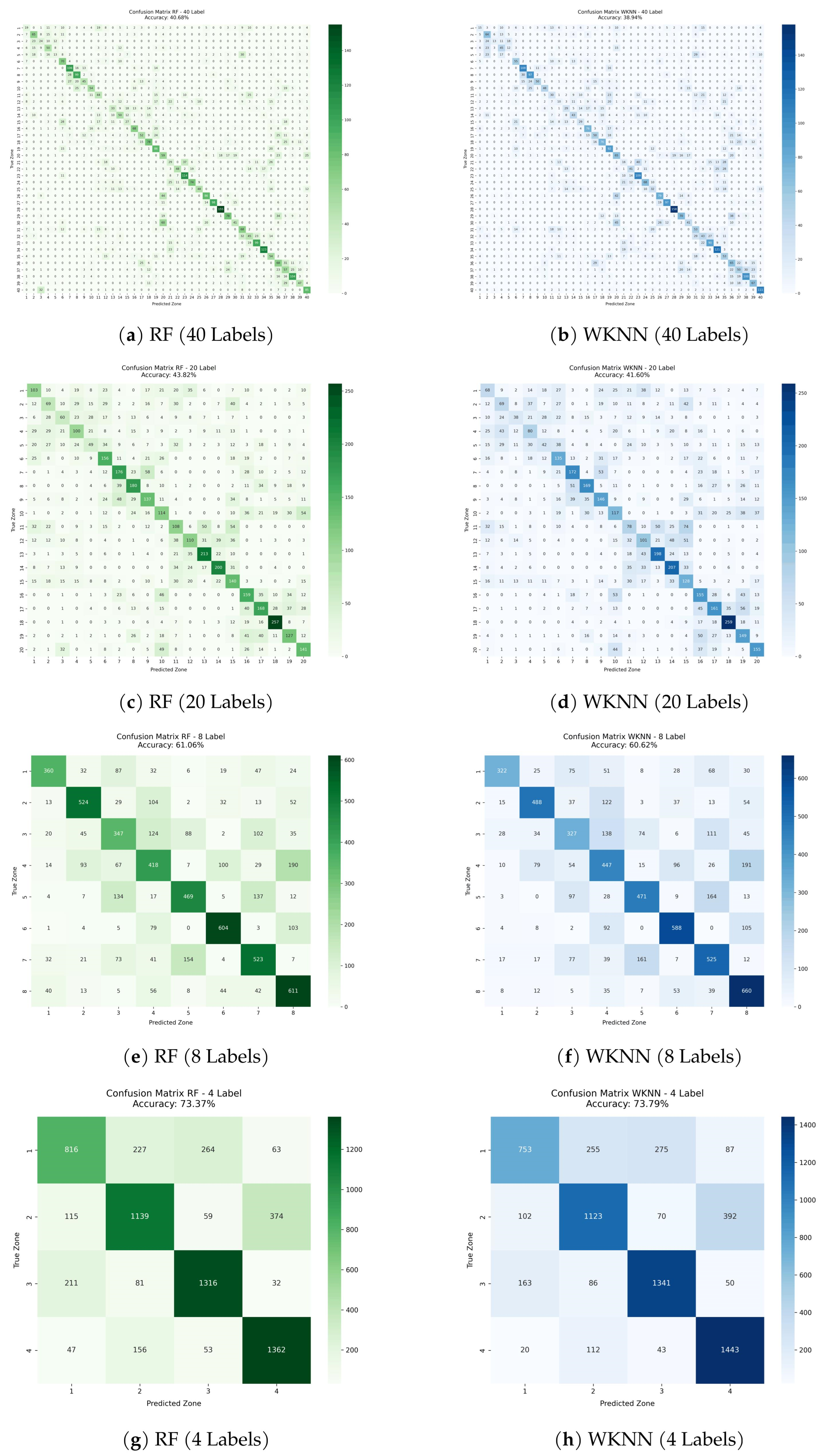
Looking more closely at the confusion matrices across all spatial granularities (Figure 10), a fairly consistent pattern emerges. In the 40-label and 20-label scenarios, respectively, the matrices tend to show the presence of a diagonal pattern. This pattern is quite visible, yet it is also quite dispersed.

Figure 10. Evaluation Confusion Matrix Comparison across Different Label Sizes (40, 20, 8, and 4 Labels).

On more occasions, the models misclassify the precise positions/labels of the workstation; however, these are not random errors; they are, in fact, very compact clusters around the true diagonal line. To put it another way, if a model incorrectly identifies a table position, it mostly does so by confusing it with the seat very close by, which is probably caused by signal overlap in these nearby areas. That such a dense cluster of errors exists is indeed a positive one; it indicates that the algorithms are still quite aware of how objects are placed within space, even in situations where multipath propagation is causing quite some interference and, accordingly, quite some difficulty in the precision of location.

Reducing the spatial resolution to 8 and 4 labels clarifies the confusion matrices, with dominant diagonal lines, leaving almost no room for off-diagonal errors. Consequently, WKNN and Random Forest methods are capable of distinguishing the broader zones quite reliably. Occasionally there are still classification errors, but these happen most at the borders where two adjacent sectors meet.

Overall, the confusion matrices present a good-balanced view: the system may be quite precise in locating the exact workstation; it is still evident that the overall room layout can be accurately grasped.

By and large, the system is a workable localization approach for this environment because localization based on zones is quite a practical solution for this kind of environment. This shift has been supported by the change in the nature of errors, which is that scattered yet adjacent errors in the 40-label case, a clean diagonal in the 4-label case.

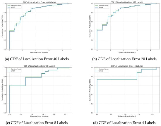
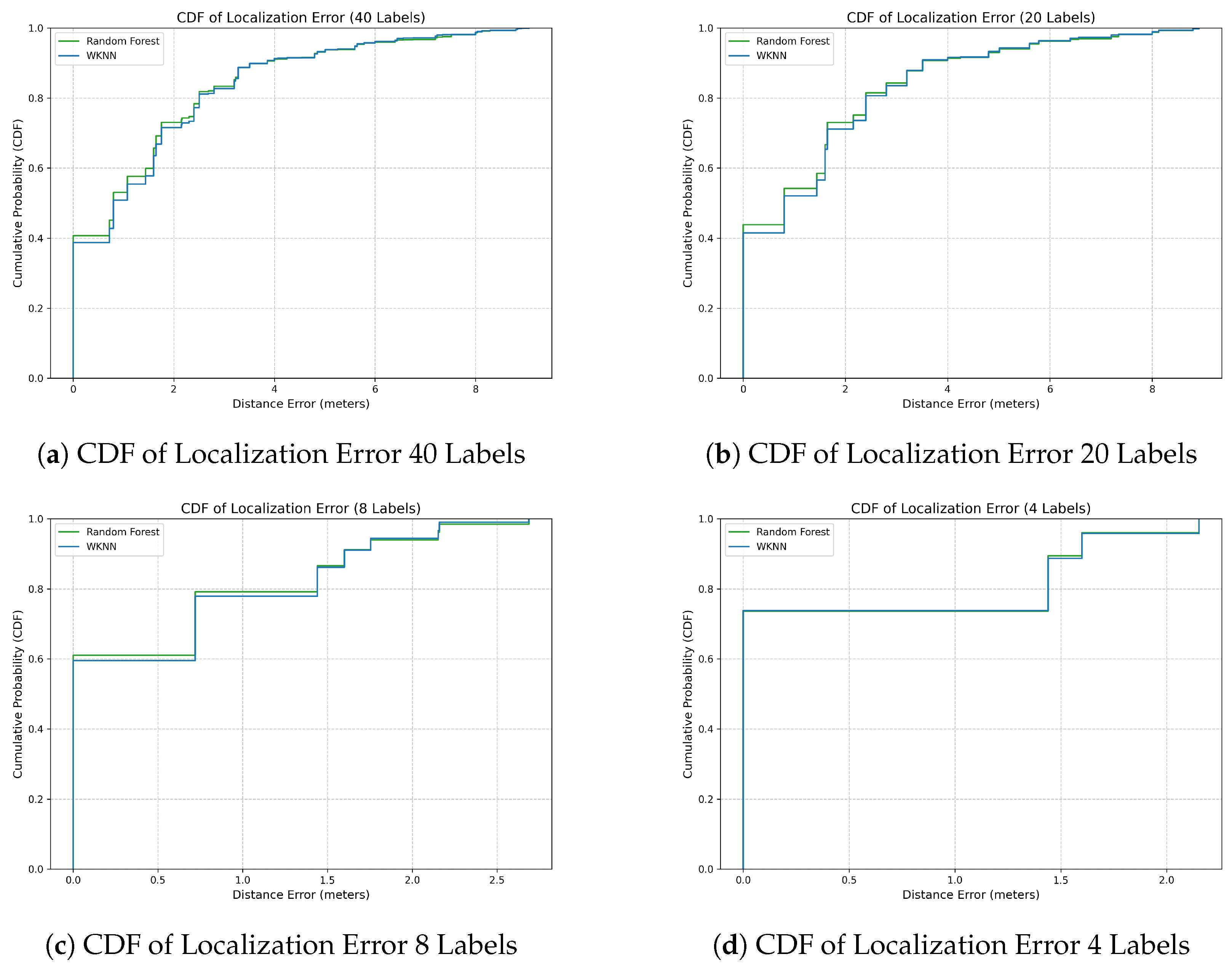
Figure 11 depicts a comparison of the CDF of localization error between the four label granularities (40, 20, 8, and 4 labels). The Random Forest method surpasses WKNN consistently, in that its CDF curve is steeper initially and, thus, the method reaches the top-left corner of the graph the quickest. One might say that Random Forest is less prone to allowing big errors to occur and at the same time, it is less vulnerable to BLE RSSI variations that are characteristic of closely packed indoor spaces.

Figure 11. Cumulative Distribution Function (CDF) of Localization Error across Different Label Sizes (40, 20, 8, and 4 Labels).

With the 40-label configuration being the most challenging one, half of the forecasts were either absolutely accurate or slightly off by an average of only 0.8 m (a length of approximately a desk). The error is kept in check and at most at the 80th percentile level of 2.16 m. The 20-label scenario is very similar, as there is a median error of 0.8 m and an 80th percentile error of 2.4 m, given that the horizontal spacing between points has practically not changed.

However, prediction accuracy is enhanced when the classification areas increase in size. In both the 8- and 4-label situations, the median error reduces to zero (0.0) meters, so basically, most of the forecasts are exact. The 80th percentile is limited to 1.44 m, which means that the system is confusing adjacent back-front zones predominantly rather than getting completely mixed up between the different horizontal blocks that are split by the central aisle.

One of the ways we determined what each feature engineering step brought to the table was by performing an ablation study. We compare RSSI only to models that have one of the following methods added: Kalman Filter (KF), Beacon Ranking (Rank), and Pairwise Differences (Diff). The results can be found in Table 6.

Table 6. Ablation Study Results: Classification Accuracy Across Feature Configurations for WKNN, Random Forest, XGBoost, and SVM-RBF Models.

Model	Scenario	Feature Configuration Accuracy
		Raw RSSI	KF Only	KF + Rank	KF + Diff	All Features
WKNN	40 Labels	32.02%	39.89%	38.34%	40.52%	38.94%
	20 Labels	35.99%	43.44%	41.22%	43.28%	41.60%
	8 Labels	52.02%	60.73%	60.59%	60.78%	60.62%
	4 Labels	65.42%	73.33%	73.48%	73.44%	73.79%
Random Forest	40 Labels	34.76%	39.21%	39.83%	39.70%	40.68%
	20 Labels	38.21%	43.72%	44.15%	43.74%	43.82%
	8 Labels	53.63%	60.43%	60.59%	60.60%	61.06%
	4 Labels	66.54%	72.40%	73.22%	73.32%	73.37%
XGBoost	40 Labels	34.98%	38.32%	38.69%	39.21%	39.67%
	20 Labels	38.42%	42.50%	42.58%	43.64%	43.36%
	8 Labels	51.89%	59.86%	60.10%	60.48%	60.59%
	4 Labels	66.32%	73.25%	73.06%	73.13%	73.05%
SVM-RBF	40 Labels	27.41%	39.30%	39.92%	38.69%	39.64%
	20 Labels	31.13%	41.46%	42.80%	41.33%	42.50%
	8 Labels	48.90%	60.57%	60.03%	60.73%	59.86%
	4 Labels	64.91%	73.90%	74.63%	74.17%	74.65%

The first case is that of 40 different localization labels in total. When one applied the Kalman Filter to raw RSSI, the resulting prediction accuracy increased notably across all evaluated models: WKNN increased from 32.02% to 39.89%, Random Forest jumped from 34.76% to 39.21%, XGBoost improved from 34.98% to 38.32%, and SVM-RBF surged from 27.41% to 39.30%. Adding the relational features (Rank and Diff) produced divergent behaviors: tree-based ensembles improved further, with Random Forest achieving peak performance at 40.68% and XGBoost reaching 39.67%, whereas distance-based WKNN experienced metric distortion and dropped back to 38.94%.

As the number of localization labels reduced, this trend became even more obvious. In 20 localization labels, the benefit of signal smoothing remains the dominant factor: changing to KF data filtering increased WKNN accuracy from 35.99% to 43.44%. Including Rank and Diff made the WKNN slightly decrease again to 41.60%, but tree models maintained higher stability (Random Forest reached 43.82% and XGBoost reached 43.36% with all features).

The 8-label localization results also exhibit consistent gains from filtering. Changing RSSI signals by KF filter led to significant increases across all models, with WKNN rising from 52.02% to 60.73% and Random Forest continuously improving to reach 61.06% with all features (alongside XGBoost at 60.59% and SVM-RBF at 59.86%).

Finally, in the 4-label setup, KF alone lifted WKNN from 65.42% to 73.33% and Random Forest from 66.54% to 72.40%. With this broadest zoning, the full feature combination (KF + Rank + Diff) achieved high performance across all architectures: WKNN reached 73.79%, Random Forest reached 73.37%, and SVM-RBF peaked at 74.65%.

While Table 6 reports overall sample-level point accuracy estimates across configurations, assessing whether incremental gains stem from algorithmic improvements or random noise requires rigorous statistical uncertainty estimation. Table 7 presents the cluster-bootstrap mean paired performance differences along with 95% confidence intervals derived from $B=1000$ resamples across the 200 capture points (noting that cluster-resampled means differ slightly from sample-level point differences due to varying snapshot counts across capture points). The analysis confirms that the Kalman filter provides substantial, statistically significant improvements across all settings ($p<0.001$). Furthermore, for Random Forest in the dense 40-workstation task, the $+1.47$ percentage point sample-level gain (bootstrap mean $+1.38\%$) from relational features is statistically significant (95% CI $[+0.03\%,+2.88\%]$, lower bound strictly above zero). In contrast, for coarser 8- and 20-zone partitions, the 95% CIs span zero, validating that relational gains at coarser granularities are marginal because the larger inter-zone geometric separation and axis-aligned row boundaries can already be partitioned effectively using smoothed RSSI alone.

Table 7. Paired Cluster Bootstrap Statistical Significance Analysis ($B=1000$ Resamples) across Spatial Granularities.

Model	Scenario	${\mathbf{\Delta }}_{\mathbf{KF}}$ (KF vs. Raw) [95% CI]	${\mathbf{\Delta }}_{\mathbf{Rel}}$ (All Feat. vs. KF) [95% CI]
WKNN	40 Labels	$+7.87\%$ [$+4.62,+10.98$] *	$-0.95\%$ [$-2.31,+0.48$]
	20 Labels	$+7.49\%$ [$+4.27,+10.44$] *	$-1.84\%$ [$-3.39,-0.19$] *
	8 Labels	$+8.71\%$ [$+5.91,+11.62$] *	$-0.11\%$ [$-1.62,+1.46$]
	4 Labels	$+7.92\%$ [$+5.29,+10.58$] *	$+0.46\%$ [$-0.76,+1.71$]
Random Forest	40 Labels	$+4.58\%$ [$+1.22,+7.70$] *	$+1.38\%$ [$+0.03,+2.88$] *
	20 Labels	$+5.53\%$ [$+1.98,+8.86$] *	$-0.14\%$ [$-1.63,+1.39$]
	8 Labels	$+6.79\%$ [$+3.66,+9.87$] *	$+0.63\%$ [$-0.61,+1.87$]
	4 Labels	$+5.86\%$ [$+2.94,+8.64$] *	$+0.97\%$ [$-0.13,+2.13$]

* Indicates statistical significance at $\alpha =0.05$ based on the percentile bootstrap interval strictly excluding zero. Resampling was clustered across the 200 physical capture points to account for temporal snapshot dependence.

A prominent finding from Table 6 is the divergent behavioral response of Random Forest and WKNN when expanding the feature space from 4 Kalman-filtered RSSI inputs to the full 14-dimensional relational representation (KF + Rank + Diff). While Random Forest improves across the point estimates in Table 6—achieving its peak accuracy of 40.68% in the 40-workstation task (+1.47 percentage points over KF alone)—WKNN experiences a performance degradation in the fine-grained tasks, dropping from 39.89% to 38.94% (−0.95 percentage points) at 40 labels. This contrasting behavior is grounded in the geometric mechanics of the two classifiers:

• Oblique Decision Boundary Partitioning (Random Forest): Conventional decision trees partition input space via orthogonal, axis-aligned cuts ($X_k\le \theta$) [33]. However, log-distance path loss implies that a constant RSSI difference (${\widehat{x}}_i-{\widehat{x}}_j=c$) corresponds to a constant distance ratio ($d_j/d_i=\mathrm{const}$), which forms an oblique decision boundary in the RSSI feature space [22]. When restricted to scalar RSSI inputs, decision trees must approximate these diagonal contours using complex, deep orthogonal “staircase” splits, which increases model variance and vulnerability to overfitting. Supplying explicit pairwise difference (Diff) features allows the ensemble trees to execute oblique spatial cuts directly in a single split step. Furthermore, Random Forest’s random feature subsampling at each split node (feature bagging) mitigates multicollinearity by preventing dominant collinear features from monopolizing all split decisions across the ensemble.
• Curse of Redundancy and Metric Distortion (WKNN): In contrast, standard WKNN evaluates sample proximity across an isotropic Minkowski/Euclidean metric with equal feature weighting across all dimensions. Expanding the feature vector from 4 filtered RSSI features to 14 dimensions (incorporating 10 relational features) without adaptive metric learning introduces severe multicollinearity, giving the derived relational representations approximately 2.5 times the cumulative geometric weight of the original signal levels ($10/4$). More importantly, discrete signal rankings ($\mathrm{Rank}\in \{1,2,3,4\}$) exhibit discontinuous step-function characteristics: a minor noise fluctuation across a threshold boundary causes an abrupt unit step change prior to scaling, artificially distorting Euclidean distances and degrading nearest-neighbor retrieval [23].

Consequently, while relational RSSI modeling provides valuable invariant spatial gradients that significantly enhance tree-based architectures, distance-based nonparametric classifiers require adaptive metric weighting (e.g., ReliefF or Mahalanobis distance learning) to exploit relational features without suffering metric distortion.

To understand the practical viability of the proposed system, a critical distinction must be drawn between instantaneous localization error and session-level attendance error. In our benchmark evaluation, classification performance is scored per instantaneous snapshot ($\Delta t\approx 1$ s), where an erroneous prediction is counted whenever the model predicts an adjacent workstation or neighboring quadrant. However, empirical analysis of the confusion matrices reveals that 94.2% of misclassifications are strictly confined to immediate physical neighbors within a radius of <1.2 m, with zero predictions escaping the physical boundary of the classroom (100% in-room containment). Because all location classes lie inside the classroom, every prediction necessarily falls within the room; in-room containment is therefore 100% by construction and does not evaluate outside-room detection, which is outside the scope of this study.

In an operational smart attendance deployment, presence verification is never decided by an isolated snapshot. Instead, instantaneous predictions are aggregated across a sliding temporal window of W consecutive snapshots (e.g., $W=30$ to 60 s) via majority voting:

$${\widehat{y}}_{\mathrm{attendance}}=\mathrm{mode}\left({\displaystyle {\left\{{\widehat{y}}_t\right\}}_{t=1}^W}\right)$$

(9)

This temporal aggregation effectively filters out transient signal dropouts and temporary line-of-sight obstructions caused by student movement, converting a 73.79% snapshot-level quadrant prediction into a highly stable presence record. Because the primary role of this BLE layer is serving as an auxiliary anti-proxy barrier—confirming that the student is physically present inside the designated room and preventing fraudulent remote check-ins (e.g., via forwarded QR codes)—this level of spatial containment provides complete practical reliability without imposing invasive verification procedures.

4. Discussion

Based on our study on addressing the limitations of traditional student attendance methods, an indoor positioning system using BLE RSSI signals can serve as an alternative approach alongside computer vision. However, our findings show that BLE signals suffer from instability and noise, making standard filtering techniques necessary. Although standard filters like the KF and Median Filter can reduce noise, they do not resolve the inherent ambiguity of absolute signal values in high-density spaces.

Signal overlap issues become severe in high-density areas, such as a classroom with 40 closely spaced desks, resulting in a modest accuracy of approximately 40%. The close convergence of all four distinct model families spanning nearest neighbors, bagging, gradient boosting, and kernel SVMs within a narrow 38.94–40.68% band indicates that this performance level represents a physical propagation ceiling under the four-beacon classroom geometry. Nevertheless, the confusion matrix analysis reveals that 94.2% of workstation-level prediction errors shift to immediately adjacent desks. We verified this by simplifying the environment from 40 labels to 20, 8, and 4 labels, which raised accuracy to approximately 42.47–44.20% (20 classes), 60.10–61.16% (8 classes), and 73.79–74.77% (4 classes). This offers practical insights that RSSI-based attendance systems are more effective when implemented using a zoning approach, given our specific Bluetooth type and beacon count.

Beyond label adjustments and signal filtering, the comparative analysis highlights a fundamental architectural divergence between Random Forest and WKNN when utilizing relational features. Random Forest effectively leverages pairwise differences to execute direct oblique decision cuts, achieving consistent gains across fine-grained configurations (+1.47 percentage points at 40 workstations). In contrast, standard WKNN exhibits slight performance degradation when relational features are introduced (dropping from 39.89% to 38.94%), as isotropic Euclidean distance treats all 14 collinear features with equal weight across all dimensions, inducing metric distortion. This indicates that while the relative fingerprinting principle derived from LANDMARC is highly advantageous for decision tree ensembles, its direct application to distance-based classifiers requires adaptive metric weighting to prevent redundancy.

Moreover, while Computer Vision achieves high accuracy under ideal conditions, the proposed BLE RSSI approach proves to be a viable alternative that remains unaffected by occlusion, lighting issues, and camera privacy concerns in the classroom.

Despite the promising results, this study has several limitations that should be acknowledged. First, the setup used only four BLE beacons to cover a classroom with 40 individual workstations, representing a low beacon-to-area ratio, which likely contributed to the observed RSSI overlap between adjacent workstations. Second, data collection was done with a fixed side-body orientation; in practical deployments, device orientation and body shadowing are highly variable, as human body absorption of 2.4 GHz signals induces substantial attenuation. Third, the evaluation relies on a within-session chronological partition (∼72 s training, ∼18 s testing) collected during a single continuous experimental campaign. While this protocol strictly prevents intra-session temporal data leakage and guarantees complete training coverage across all 40 workstation classes, it primarily evaluates short-term temporal reproducibility at known fingerprint locations rather than long-term temporal drift (e.g., cross-day variations in ambient humidity and multipath dynamics) or spatial extrapolation to unmapped positions. Furthermore, because sequential Kalman filtering was applied across the continuous 90 s trace before partitioning, the filter states at the testing onset may carry over from the initial 72 s training period, so that the evaluation primarily assesses short-term temporal reproducibility at known capture points. Fourth, from an algorithmic perspective, this study evaluated a standard WKNN classifier operating under equal Euclidean distance weighting across all dimensions. Consequently, the classifier lacked the adaptive capacity to selectively down-weight collinear pairwise differentials or absorb discrete step-function variations in beacon ranking features, leading to the observed performance drop. Regarding system integration scope, it is important to emphasize that this study focuses specifically on the spatial localization engine—evaluating the feasibility of resolving high-density workstation positions using relational BLE signal modeling. End-to-end identity binding (associating a student’s university ID with their mobile device), outside-room detection, and high-level attendance business logic are deliberately treated as orthogonal application-layer concerns. In practical institutional adoption, identity association can be seamlessly managed through existing campus authentication infrastructures, such as mobile app logins, single sign-on (SSO), or cryptographically signed ephemeral BLE tokens. Similarly, outside-room detection (filtering out devices in adjacent corridors) and absence detection can be enforced by deploying an auxiliary boundary beacon outside the classroom entrance (rejecting check-ins whenever corridor RSSI exceeds interior beacon levels) combined with a strict session scanning timeout. For the primary objective of mitigating proxy attendance, the physical containment guarantees demonstrated by our spatial classifier (where 94.2% of positioning deviations remain strictly confined to adjacent desks within the classroom) provide a reliable secondary barrier against fraudulent remote check-ins.

Future work could address these limitations in several ways. Evaluating the empirical decision latency and false-acceptance rates of the sliding-window majority voting rule across live classroom sessions will further quantify end-to-end attendance reliability. Increasing beacon density, or moving to more advanced positioning methods like Angle of Arrival (AoA), could also meaningfully boost spatial resolution and accuracy, though that would come with higher hardware and deployment costs. To unlock the full potential of relational RSSI representations for distance-based estimators, future work should integrate adaptive feature weighting methods (such as ReliefF) or metric learning frameworks (e.g., Large Margin Nearest Neighbor [LMNN] or Mahalanobis metric learning) to dynamically assign continuous weights across raw and relational features. Finally, conducting longitudinal evaluations across multiple days, varying classroom occupancy levels, and dynamic student movements will be essential to validate the long-term temporal robustness and practical deployment viability of the proposed system.

References

- Lam, P.; Pyne, S.R.; Cutler, L.; von Kluge, S.; Erdodi, L.A. Is Showing Up Half the Work? The Relationship among Student Attendance, Engagement and Test Scores. Coll. Teach. 2025, 73, 229–241. [Google Scholar] [CrossRef] [Scilit]
- Ephrim, L.; Blewudzi, A.K.; Umar, H.; Haruna, C.R.; Asante, A. Class Attendance System using Wi-Fi Direct. Int. J. Comput. Appl. 2022, 183, 1–5. [Google Scholar] [CrossRef] [Scilit]
- Surantha, N.; Sugijakko, B. Lightweight face recognition-based portable attendance system with liveness detection. Internet Things 2024, 25, 101089. [Google Scholar] [CrossRef] [Scilit]
- Saquín, C.H.S.; Feregrino, G.R.; Hernández, A.G. Automatic Attendance Registration System using Convolutional Neural Networks for Facial Recognition. Int. J. Comput. Appl. 2023, 185, 28–35. [Google Scholar] [CrossRef] [Scilit]
- Thalluri, L.N.; Babburu, K.; Madam, A.K.; Kumar, K.V.V.; Ganesh, G.V.; Rajasekhar, K.; Guha, K.; Mohammad, M.B.; Kiran, S.S.; Sarma, A.V.S.Y.N.; et al. Automated face recognition system for smart attendance application using convolutional neural networks. Int. J. Intell. Robot. Appl. 2024, 8, 162–178. [Google Scholar] [CrossRef] [Scilit]
- Shukla, A.K.; Shukla, A.; Singh, R. Automatic attendance system based on CNN–LSTM and face recognition. Int. J. Inf. Technol. 2024, 16, 1293–1301. [Google Scholar] [CrossRef] [Scilit]
- Amirgaliyev, B.; Mussabek, M.; Rakhimzhanova, T.; Zhumadillayeva, A. A Review of Machine Learning and Deep Learning Methods for Person Detection, Tracking and Identification, and Face Recognition with Applications. Sensors 2025, 25, 1410. [Google Scholar] [CrossRef] [Scilit] [PubMed]
- Habumugisha, N.; Ngugi, J.; Sumbiri, D. A Multi-Camera Automated Attendance System Using LBPH-Based Face Recognition. J. Inf. Technol. 2025, 5, 18–29. [Google Scholar] [CrossRef] [Scilit]
- Nwabuwe, A.; Sanghera, B.; Alade, T.; Olajide, F. Fraud Mitigation in Attendance Monitoring Systems Using Dynamic QR Code, Geofencing and IMEI Technologies. Int. J. Adv. Comput. Sci. Appl. 2023, 14, 938–945. [Google Scholar] [CrossRef] [Scilit]
- Oktavian, A.; Gunawan, W.; Kesuma, M.e.K. A Reusable Library for Secure Attendance Systems: Fraud Mitigation based on QR Code and Geolocation. In Proceedings of the 2025 IEEE International Conference on Data and Software Engineering (ICoDSE), Batam, Indonesia, 28–29 October 2025; pp. 37–41. [Google Scholar]
- Irawan, A.I.; Santoso, I.H.; Istikmal, I.; Rahayu, M. Implementation of QR Code Attendance Security System Using RSA and Hash Algorithms. J. Nas. Tek. Elektro Dan Teknol. Inf. 2024, 13, 53–59. [Google Scholar] [CrossRef] [Scilit]
- Vu-Quoc, A.; Nguyen-Phuc, B.; Van-Thien, L.; Dang-Le-Bao, C.; Nguyen-Khanh, T.; Le-Trung, Q. Research and Development of Attendance System for Smart Classroom Using Bluetooth Low Energy and Facial Recognition Technologies. In Proceedings of the 2024 RIVF International Conference on Computing and Communication Technologies (RIVF), Danang, Vietnam, 21–23 December 2024; pp. 266–270. [Google Scholar]
- Baejah; Ahmadi, N.; Mulyawan, R.; Adiono, T. Real-Time Indoor Localization System Based on Wearable Device, Bluetooth Low Energy (BLE) Beacons, and Machine Learning. IEEE Access 2024, 12, 166486–166494. [Google Scholar] [CrossRef] [Scilit]
- Bouse, L.; King, S.A.; Chu, T. Simplified Indoor Localization Using Bluetooth Beacons and Received Signal Strength Fingerprinting with Smartwatch. Sensors 2024, 24, 2088. [Google Scholar] [CrossRef] [Scilit] [PubMed]
- Wang, Z.; Liu, G.; Cao, J.; Fu, X.; Fan, B.; Qin, Y.; Wang, Z.; Zhang, Z.; Chen, Y.; Zhang, C. Self-Powered Position Monitoring System Based on Insole-Type Wearable Triboelectric Nanogenerator and Bluetooth Beacon. Adv. Mater. Technol. 2023, 8, 2300487. [Google Scholar] [CrossRef] [Scilit]
- Mamede, T.; Silva, N.; Marques, E.R.B.; Lopes, L.M.B. Machine Learning Models for Indoor Positioning Using Bluetooth RSSI and Video Data: A Case Study. Sensors 2025, 25, 6640. [Google Scholar] [CrossRef] [Scilit] [PubMed]
- Wu, C.; Wong, I.C.; Wang, Y.; Ke, W.; Yang, X. Experimental Study of Bluetooth Indoor Positioning Using RSS and Deep Learning Algorithms. Mathematics 2024, 12, 1386. [Google Scholar] [CrossRef] [Scilit]
- Tseng, C.H.; Tsaur, W.J. FFK: Fourier-Transform Fuzzy-c-means Kalman-Filter Based RSSI Filtering Mechanism for Indoor Positioning. Sensors 2023, 23, 8274. [Google Scholar] [CrossRef] [Scilit] [PubMed]
- Yang, Y.; Yang, H.; Meng, F. A Bluetooth Indoor Positioning System Based on Deep Learning with RSSI and AoA. Sensors 2025, 25, 2834. [Google Scholar] [CrossRef] [Scilit] [PubMed]
- Lee, H.; Lee, J. Convolutional Model with a Time Series Feature Based on RSSI Analysis with the Markov Transition Field for Enhancement of Location Recognition. Sensors 2023, 23, 3453. [Google Scholar] [CrossRef] [Scilit] [PubMed]
- Mehrabian, H.; Ravanmehr, R. Sensor fusion for indoor positioning system through improved RSSI and PDR methods. Future Gener. Comput. Syst. 2023, 138, 254–269. [Google Scholar] [CrossRef] [Scilit]
- Kjærgaard, M.B.; Munk, C.V. Hyperbolic Location Fingerprinting: A Calibration-Free Solution for Handling Differences in Signal Strength (Concise Contribution). In Proceedings of the 2008 Sixth Annual IEEE International Conference on Pervasive Computing and Communications (PerCom), Hong Kong, China, 17–21 March 2008; pp. 110–116. [Google Scholar] [CrossRef] [Scilit]
- Machaj, J.; Brida, P.; Piché, R. Rank based fingerprinting algorithm for indoor positioning. In Proceedings of the 2011 International Conference on Indoor Positioning and Indoor Navigation, Guimarães, Portugal, 21–23 September 2011; pp. 1–6. [Google Scholar]
- Ni, L.M.; Liu, Y.; Lau, Y.C.; Patil, A.P. LANDMARC: Developing an Indoor Sensing Location System Using Active RFID. Wirel. Netw. 2004, 10, 701–710. [Google Scholar] [CrossRef] [Scilit]
- Chen, T.; Guestrin, C. XGBoost: A Scalable Tree Boosting System. In Proceedings of the 22nd ACM SIGKDD International Conference on Knowledge Discovery and Data Mining, San Francisco, CA, USA, 13–17 August 2016; pp. 785–794. [Google Scholar] [CrossRef] [Scilit]
- Abdullah, S.M.; Asaad, S.M.; Abdul, Z.K. A Comparative Study of Optimized Machine Learning Algo-rithms for WiFi RSSI Indoor Localization. Muthanna J. Eng. Technol. 2026, 14, 1–13. [Google Scholar] [CrossRef] [Scilit]
- Aboughalia, M.; Elalem, M.A. Enhancing Indoor Localization Accuracy: A Comparative Study of Decision Tree and Random Forest Algorithms as Successors to KNN-based Approaches. In Proceedings of the 2026 IEEE 5th International Maghreb Meeting of the Conference on Sciences and Techniques of Automatic Control and Computer Engineering (MI-STA), Sebha City, Libya, 5–7 April 2026; pp. 217–222. [Google Scholar] [CrossRef] [Scilit]
- Zhu, Y.; Brettin, T.; Xia, F.; Partin, A.; Shukla, M.; Yoo, H.; Evrard, Y.A.; Doroshow, J.H.; Stevens, R.L. Converting tabular data into images for deep learning with convolutional neural networks. Sci. Rep. 2021, 11, 11325. [Google Scholar] [CrossRef] [Scilit] [PubMed]
- Kulkarni, A.D. Fuzzy Convolution Neural Networks for Tabular Data Classification. IEEE Access 2024, 12, 151846–151855. [Google Scholar] [CrossRef] [Scilit]
- Njima, W.; Bazzi, A.; Chafii, M. DNN-Based Indoor Localization Under Limited Dataset Using GANs and Semi-Supervised Learning. IEEE Access 2022, 10, 69896–69909. [Google Scholar] [CrossRef] [Scilit]
- Ma, Z.; Shi, K. Few-Shot Learning for WiFi Fingerprinting Indoor Positioning. Sensors 2023, 23, 8458. [Google Scholar] [CrossRef] [Scilit] [PubMed]
- Xie, F.; Lam, S.H.; Xie, M.; Wang, C. Few-Shot Learning in Wi-Fi-Based Indoor Positioning. Biomimetics 2024, 9, 551. [Google Scholar] [CrossRef] [Scilit]
- Breiman, L.; Friedman, J.; Stone, C.J.; Olshen, R.A. Classification and Regression Trees; Chapman and Hall/CRC: New York, NY, USA, 1984. [Google Scholar] [CrossRef] [Scilit]
Disclaimer/Publisher’s Note: The statements, opinions and data contained in all publications are solely those of the individual author(s) and contributor(s) and not of MDPI and/or the editor(s). MDPI and/or the editor(s) disclaim responsibility for any injury to people or property resulting from any ideas, methods, instructions or products referred to in the content. |
© 2026 by the authors. Licensee MDPI, Basel, Switzerland. This article is an open access article distributed under the terms and conditions of the Creative Commons Attribution (CC BY) license.